Economics 2535 Lecture Notes Advanced Topics in ... - CiteSeerX
Economics 2535 Lecture Notes Advanced Topics in ... - CiteSeerX
Economics 2535 Lecture Notes Advanced Topics in ... - CiteSeerX

You also want an ePaper? Increase the reach of your titles
YUMPU automatically turns print PDFs into web optimized ePapers that Google loves.
<strong>Economics</strong> <strong>2535</strong> <strong>Lecture</strong> <strong>Notes</strong><br />
<strong>Advanced</strong> <strong>Topics</strong> <strong>in</strong> International Trade: Firms and<br />
International Trade<br />
Pol Antràs<br />
Harvard University Department of <strong>Economics</strong><br />
Spr<strong>in</strong>g 2004
Contents<br />
1 Introduction and Basic Facts 4<br />
I Firms and the Decision to Export 12<br />
2 Intra<strong>in</strong>dustry Heterogeneity with Fixed Costs of Export<strong>in</strong>g: Melitz<br />
(2003) 13<br />
3 Intra<strong>in</strong>dustry Heterogeneity and Bertrand Competition: Bernard,<br />
Eaton, Jensen, and Kortum (2003) 27<br />
4 Firms and the Decision to Export: Empirics 38<br />
4.1 Export<strong>in</strong>gandPlant-LevelPerformance.................. 38<br />
4.2 Evidence on Reallocation Effects:Pavcnik(2002) ............ 40<br />
5 The Relevance of Sunk Costs 47<br />
II Firms and the Decision to Invest Abroad 52<br />
6 Horizontal FDI: Bra<strong>in</strong>ard (1997) 53<br />
7 Exports vs. FDI with Asymmetric Countries: Markusen and Venables<br />
(2000) 63<br />
8 Exports vs. FDI with Heterogenous Firms: Helpman, Melitz and<br />
Yeaple (2003) 71<br />
9 VerticalFDI:TheoryandEvidence 82<br />
1
III Intermission: The Boundaries of The Firm 96<br />
10 The Theory of The Firm: Transaction-Cost Approaches 97<br />
11 The Theory of The Firm: The Property-Rights Approach 107<br />
12 The Theory of The Firm: Alternative Approaches 120<br />
12.1 The Firm as an Incentive System: Holmstrom and Milgrom (1994) . . . 120<br />
12.2FormalandRealAuthority:AghionandTirole(1997) ......... 126<br />
12.3AuthorityandHierarchies:Rosen(1982) ................. 129<br />
IV Trade and Organizational Form 137<br />
13 Early Transaction-Cost Approaches 138<br />
13.1Ethier(1986) ................................ 138<br />
13.2EthierandMarkusen(1996)........................ 144<br />
14 The Transaction-Cost Approach <strong>in</strong> Industry Equilibrium: McLaren<br />
(2000) and Grossman and Helpman (2002) 148<br />
14.1GlobalizationandVerticalStructure:McLaren(2000).......... 148<br />
14.2 Integration vs. Outsourc<strong>in</strong>g <strong>in</strong> Industry Equilibrium: Grossman and<br />
Helpman(2002)............................... 154<br />
15 The Property-Rights Approach <strong>in</strong> International Trade (I): Antràs<br />
(2003a) 165<br />
16 The Property-Rights Approach <strong>in</strong> International Trade (II): Antràs<br />
(2003b) and Antràs and Helpman (2004) 182<br />
16.1 Incomplete Contracts and the Product Cycle: Antràs (2003b) ..... 183<br />
16.2 Global Sourc<strong>in</strong>g with Heterogenous Firms: Antràs and Helpman (2004) 194<br />
2
Preface<br />
These lecture notes review some of the material that I cover <strong>in</strong> the advanced graduate<br />
course <strong>in</strong> the International Trade that I teach at Harvard University. The course focuses<br />
on a firm-level approach to <strong>in</strong>ternational trade and on selected topics <strong>in</strong> trade policy.<br />
I am teach<strong>in</strong>g this class for the firsttimethisSpr<strong>in</strong>g,sothenotesarelikelytoconta<strong>in</strong><br />
several typos and mistakes. Comments, suggestions, and corrections would be most<br />
welcome.<br />
Pol Antràs<br />
Department of <strong>Economics</strong><br />
Harvard University<br />
January 2004<br />
3
Chapter 1<br />
Introduction and Basic Facts<br />
• In Neoclassical Trade Theory, firms are treated as a black box. The supply<br />
side of the economy is characterized by a set of production functions accord<strong>in</strong>g to<br />
which the factors of production (capital, labor) are transformed <strong>in</strong>to consumption<br />
goods.<br />
• Moreover, for the most part, the literature assumes constant returns to scale,<br />
under which the size of the firm is <strong>in</strong>determ<strong>in</strong>ate (the general equilibrium only<br />
p<strong>in</strong>s down the size of the sector or <strong>in</strong>dustry to which the firm belongs).<br />
• New Trade Theory <strong>in</strong>troduced <strong>in</strong>creas<strong>in</strong>g returns and imperfect competition <strong>in</strong><br />
<strong>in</strong>ternational trade. This resolved the <strong>in</strong>determ<strong>in</strong>acy of the size of the firm. As an<br />
example, take a Helpman-Krugman type of model with product differentiation.<br />
The unique producer of a particular variety ω faces demand given by:<br />
q (ω) =Ap (ω) −ε , ε>1<br />
and hence sets q (ω) to maximize:<br />
π (ω) =A 1/ε q (ω) (ε−1)/ε − q (ω)<br />
ϕ − f,<br />
where 1/ϕ is the marg<strong>in</strong>al cost of production and f is a fixed cost. Profits are<br />
strictly concave <strong>in</strong> q (ω), so there is a well-determ<strong>in</strong>ed profit-maximiz<strong>in</strong>g level of<br />
output q ∗ (ω).<br />
4
• Still, as discussed below, New Trade Theory cannot account for important facts<br />
<strong>in</strong> the data.<br />
A. Firms and the Decision to Export<br />
• The Helpman-Krugman models feature complete specialization: each <strong>in</strong>dustry<br />
variety is produced by a s<strong>in</strong>gle firm <strong>in</strong> just one country, which exports its outputeverywhereelse<strong>in</strong>theworld.<br />
Add<strong>in</strong>g transport costs could potentially<br />
<strong>in</strong>validate this, but not if transport costs are of the iceberg type. In that case,<br />
we still get a similar result (the elasticity of demand rema<strong>in</strong>s unaffected). The<br />
transport cost <strong>in</strong>flates the marg<strong>in</strong>al cost and reduces profits on foreign sales:<br />
π j (ω) =A 1/ε<br />
j q jj (ω) (ε−1)/ε + X k6=j<br />
A 1/ε<br />
k<br />
q jk (ω) (ε−1)/ε − 1 ϕ<br />
Ã<br />
q jj (ω)+τ X !<br />
q jk (ω) −f,<br />
k6=j<br />
but one can show that the optimal qjk ∗ (ω) satisfies<br />
A 1/ε<br />
k<br />
q∗ jk (ω) (ε−1)/ε − τ ϕ q∗ jk (ω) = 1 ε A k<br />
µ ε−1 (ε − 1) ϕ<br />
> 0 for all k 6= j.<br />
Hence, even <strong>in</strong> the presence of transport costs, a firmcont<strong>in</strong>uestoexporteverywhere<br />
else <strong>in</strong> the world. As we will see, two features of this example are crucial:<br />
(i)thattransportcostsaffect only the marg<strong>in</strong>al cost, and (ii) that foreign competition<br />
does not affect the markup the firm can charge over marg<strong>in</strong>al cost.<br />
• In reality, not all domestic producers export to foreign markets. And, more<br />
importantly, the literature has “uncovered stylized facts about the behavior and<br />
relative performance of export<strong>in</strong>g firms and plants which hold consistently across<br />
a number of countries” (Bernard et al., 2003, BEJK hereafter).<br />
— Exporters are <strong>in</strong> the m<strong>in</strong>ority. In 1992, only 21% of U.S. plants reported<br />
export<strong>in</strong>g anyth<strong>in</strong>g.<br />
— Exporters sell most of their output domestically: around 2/3 of exporters<br />
sell less than 10% of their output abroad.<br />
ετ<br />
5
— Exporters are bigger than non-exporters: they ship on average 5.6 times<br />
more than nonexporters (4.8 times more domestically).<br />
— Plants are also heterogeneous <strong>in</strong> measured productivity; Figures 2A and 2B<br />
<strong>in</strong> BEJK.<br />
— Exporters’ productivity distribution is a shift to the right of the nonexporter’s<br />
distribution. Exporters have, on average, a 33% advantage <strong>in</strong> labor<br />
productivity relative to nonexporters.<br />
— This suggests that the most productive firms self-select <strong>in</strong>to export markets,<br />
butitcouldalsoreflect learn<strong>in</strong>g by export<strong>in</strong>g (Clerides et al., 1998)<br />
• Furthermore, micro-level studies have also found evidence of substantial reallocation<br />
effects with<strong>in</strong> an <strong>in</strong>dustry follow<strong>in</strong>g trade liberalization episodes.<br />
— Exposure to trade forces the least productive firms to exit or shut-down<br />
(Bernard and Jensen, 1999; Aw, Chung and Roberts, 2000; Clerides et al.,<br />
1998).<br />
— Trade liberalization leads to market share reallocations towards more productive<br />
firms, thereby <strong>in</strong>creas<strong>in</strong>g aggregate productivity (Pavcnik, 2002,<br />
Bernard, Jensen and Schott 2003).<br />
• These studies suggest that successful theoretical frameworks for study<strong>in</strong>g firms<br />
and the decision to export should <strong>in</strong>clude two features:<br />
1. With<strong>in</strong> sectoral heterogeneity <strong>in</strong> size and productivity.<br />
2. A feature that leads only themostproductivefirms to engage <strong>in</strong> foreign<br />
trade:<br />
— This could be a sunk cost of export<strong>in</strong>g as documented by Roberts and<br />
Tybout (1997) and Bernard and Jensen (2004), and formalized by Melitz<br />
(2003);<br />
— Or a limitation on product differentiation (i.e., a fixed measure of goods)<br />
that leads to worldwide (price) competition <strong>in</strong> the production of a particular<br />
good, which <strong>in</strong> turn gives rise to variable markups (BEJK).<br />
6
• We will study each of these two approaches and revisit the empirical evidence <strong>in</strong><br />
light of the theories.<br />
B. Firms and the Decision to Invest Abroad<br />
• Another important fact that traditional trade theory neglects is that firms have<br />
(at least) two modes of servic<strong>in</strong>g a foreign market. The firstmodeistheexport<strong>in</strong>g<br />
option, which was discussed above. An alternative mode, however, is to set up<br />
multiple production plants to service the different foreign markets (i.e. engage <strong>in</strong><br />
foreign direct <strong>in</strong>vestment, FDI hereafter). This trade-off was first formalized by<br />
Markusen (1984).<br />
• Mult<strong>in</strong>ational firms may also arise when, <strong>in</strong> the presence of factor price differences<br />
across countries, a producer may f<strong>in</strong>d it optimal to fragment the production<br />
process and undertake different parts of the production process <strong>in</strong> different countries.<br />
This “vertical” approach to the mult<strong>in</strong>ational firm was first developed by<br />
Helpman (1984).<br />
• Why should we care about mult<strong>in</strong>ational firms?Becausetheyplayakeyrole<strong>in</strong><br />
the global economy:<br />
— One-third of the volume of world trade is <strong>in</strong>trafirm trade. In 1994, 42.7<br />
percent of the total volume of U.S. imports of goods took place with<strong>in</strong> the<br />
boundaries of mult<strong>in</strong>ational firms, with the share be<strong>in</strong>g 36.3 percent for U.S.<br />
exports of goods (Zeile, 1997).<br />
— About another third of the volume of world trade is accounted for by transactions<br />
<strong>in</strong> which mult<strong>in</strong>ational firms are <strong>in</strong> one of the two sides of the exchange.<br />
— Still, is this large? Rugman (1988) estimates that the largest 500 mult<strong>in</strong>ational<br />
firms account for around one-fifth of world GDP.<br />
• Furthermore, some stylized facts about mult<strong>in</strong>ational firms and FDI (Markusen<br />
1995, 2003) provide foundations for theoriz<strong>in</strong>g:<br />
I. Macro Facts<br />
7
1. FDI has grown rapidly throughout the world, especially <strong>in</strong> late 1980s and<br />
late 1990s.<br />
2. The bulk of FDI flows between developed countries. In 2000, developed<br />
countries were the source of 91 percent of FDI flows and also the recipient<br />
of 79 percent (UNCTAD, 2001). Furthermore, 80 percent of the <strong>in</strong>flows <strong>in</strong>to<br />
develop<strong>in</strong>g countries went exclusively to Hong Kong, Ch<strong>in</strong>a and Korea.<br />
3. Two-way FDI flows are common between pairs of developed countries.<br />
4.ThereexistslittleevidencethatFDIispositivelyrelatedtodifferences <strong>in</strong><br />
capital endowments across countries; see, however, Yeaple (2003).<br />
5. Political risk and <strong>in</strong>stability deter <strong>in</strong>ward FDI.<br />
II. Firm and Industry Characteristics<br />
1. The relative importance of mult<strong>in</strong>ational firms varies by <strong>in</strong>dustry. The significanceishigher<strong>in</strong>sectorsthat:<br />
— have high levels of R&D expenditures over sales<br />
— employ large number of nonproduction workers<br />
— produce new and/or complex goods<br />
— have high levels of product differentiation and advertis<strong>in</strong>g<br />
— feature high productivity dispersion (Helpman, Melitz and Yeaple, 2003)<br />
2. At the firm level, mult<strong>in</strong>ationality is:<br />
— negatively associated with plant-level scale economies<br />
— positively associated with size, up to a threshold size level<br />
— positively associated with trade barriers.<br />
• We will study different theoretical approaches to expla<strong>in</strong><strong>in</strong>g these facts. I will<br />
refer to these as technological theories of the mult<strong>in</strong>ational firm.<br />
• Of particular <strong>in</strong>terest will be the contribution by Helpman, Melitz and Yeaple<br />
(2003), which comb<strong>in</strong>es <strong>in</strong>sights from this branch of the literature together with<br />
8
<strong>in</strong>sights from the literature on with<strong>in</strong> sectoral heterogeneity and the export<strong>in</strong>g<br />
decision discussed above.<br />
• We will also briefly discuss another branch of the literature that has focused on<br />
study<strong>in</strong>g the effects of FDI.<br />
C. Firm Boundaries: Trade and Organizational Form<br />
• In recent years, we have witnessed a spectacular <strong>in</strong>crease <strong>in</strong> the way firms organize<br />
production on a global scale. Feenstra (1998), cit<strong>in</strong>g Tempest (1996), describes<br />
Mattel’s global sourc<strong>in</strong>g strategies <strong>in</strong> the manufactur<strong>in</strong>g of its star product, the<br />
Barbie doll:<br />
The raw materials for the doll (plastic and hair) are obta<strong>in</strong>ed from Taiwan and<br />
Japan. Assembly used to be done <strong>in</strong> those countries, as well as the Philipp<strong>in</strong>es,<br />
but it has now migrated to lower-cost locations <strong>in</strong> Indonesia, Malaysia, and<br />
Ch<strong>in</strong>a. The molds themselves come from the United States, as do additional<br />
pa<strong>in</strong>ts used <strong>in</strong> decorat<strong>in</strong>g the dolls. Other than labor, Ch<strong>in</strong>a supplies only the<br />
cotton cloth used for dresses. Of the $2 export value for the dolls when they<br />
leave Hong Kong for the United States, about 35 cents covers Ch<strong>in</strong>ese labor, 65<br />
cents covers the cost of materials, and the rema<strong>in</strong>der covers transportation and<br />
overheads, <strong>in</strong>clud<strong>in</strong>g profits earned <strong>in</strong> Hong Kong. (Feenstra, 1998, p. 35-36).<br />
• A variety of terms have been used to refer to this phenomenon: the “slic<strong>in</strong>g of<br />
the value cha<strong>in</strong>”, “<strong>in</strong>ternational outsourc<strong>in</strong>g”, “fragmentation of the production<br />
process”, “vertical specialization”, “global production shar<strong>in</strong>g”, and many more.<br />
• One-thirdofworldtradeis<strong>in</strong>trafirm trade, but notice that mult<strong>in</strong>ational firms<br />
choose not to <strong>in</strong>ternalize an equally sizeable volume of their transactions.<br />
In develop<strong>in</strong>g their global sourc<strong>in</strong>g strategies, firms not only decide on<br />
where to locate the differentstagesofthevaluecha<strong>in</strong>,butalsoontheextentof<br />
control they want to exert over these processes.<br />
• The <strong>in</strong>ternalization issue is noth<strong>in</strong>g more than the classical “make-or-buy”<br />
decision <strong>in</strong> <strong>in</strong>dustrial organization. Firms may decide to keep the production<br />
9
of <strong>in</strong>termediate <strong>in</strong>puts with<strong>in</strong> firm boundaries, thus engag<strong>in</strong>g <strong>in</strong> FDI when the<br />
<strong>in</strong>tegrated supplier is <strong>in</strong> a foreign country, or they may choose to contract with<br />
arm’s length suppliers for the procurement of these components. An example of<br />
the former is Intel Corporation, which assembles most of its microchips <strong>in</strong> whollyowned<br />
subsidiaries <strong>in</strong> Ch<strong>in</strong>a, Costa Rica, Malaysia, and Philipp<strong>in</strong>es. Conversely,<br />
Nike subcontracts most of the manufactur<strong>in</strong>g of its products to <strong>in</strong>dependent<br />
producers <strong>in</strong> Thailand, Indonesia, Cambodia, and Vietnam, while keep<strong>in</strong>g with<strong>in</strong><br />
firm boundaries the design and market<strong>in</strong>g stages of production.<br />
• The decision to <strong>in</strong>ternalize an <strong>in</strong>ternational transaction also seems to be systematically<br />
related to certa<strong>in</strong> <strong>in</strong>dustry and country characteristics. For <strong>in</strong>stance,<br />
Antràs (2003a) reports that the share of <strong>in</strong>trafirm imports <strong>in</strong> total U.S. imports<br />
is larger <strong>in</strong> R&D and capital <strong>in</strong>tensive sectors. In a cross-section of export<strong>in</strong>g<br />
countries, this share is also significantly larger <strong>in</strong> imports from capital-abundant<br />
countries.<br />
• Antràs (2003b) also reviews some evidence from firm-level studies that suggests<br />
that the choice between <strong>in</strong>trafirm and market transactions is significantly affected<br />
by both the degree of standardization of the good be<strong>in</strong>g produced abroad and<br />
also by the domestic firm’s resources devoted to product development.<br />
• The previously discussed approaches to the mult<strong>in</strong>ational firm share a common<br />
failure to properly model the crucial issue of <strong>in</strong>ternalization. These models can<br />
expla<strong>in</strong> why a domestic firm might have an <strong>in</strong>centive to undertake part of its<br />
production process abroad, but they fail to expla<strong>in</strong> why this foreign production<br />
will occur with<strong>in</strong> firm boundaries (i.e., with<strong>in</strong> mult<strong>in</strong>ationals), rather than<br />
through arm’s length subcontract<strong>in</strong>g or licens<strong>in</strong>g. In the same way that a theory<br />
of the firm based purely on technological considerations does not constitute<br />
a satisfactory theory of the firm (cf., Tirole, 1988, Hart, 1995), a theory of the<br />
mult<strong>in</strong>ational firm based solely on economies of scale and transport costs cannot<br />
be satisfactory either.<br />
• In this section we will <strong>in</strong>stead discuss purely organizational or contractual theories<br />
10
of the mult<strong>in</strong>ational firm.Wewillalsoreviewthetheoriesofthefirm that serve<br />
as basis for these new approaches to the mult<strong>in</strong>ational firm.<br />
• Of particular <strong>in</strong>terest will be the contribution by Antràs and Helpman (2003),<br />
which comb<strong>in</strong>es <strong>in</strong>sights from this branch of the literature together with <strong>in</strong>sights<br />
from the literature on <strong>in</strong>tra<strong>in</strong>dustry heterogeneity.<br />
11
Part I<br />
Firms and the Decision to Export<br />
12
Chapter 2<br />
Intra<strong>in</strong>dustry Heterogeneity with<br />
Fixed Costs of Export<strong>in</strong>g: Melitz<br />
(2003)<br />
• As argued <strong>in</strong> the Introduction, the available empirical studies suggest that successful<br />
theoretical frameworks for study<strong>in</strong>g firms and the decision to export should<br />
<strong>in</strong>corporate <strong>in</strong>tra<strong>in</strong>dustry heterogeneity <strong>in</strong> size and productivity. This chapter<br />
and the next present two recent theoretical frameworks that elegantly <strong>in</strong>troduce<br />
such heterogeneity <strong>in</strong> otherwise standard models of <strong>in</strong>ternational trade.<br />
• I follow Melitz <strong>in</strong> discuss<strong>in</strong>g first the closed economy model and then mov<strong>in</strong>g on<br />
to the open economy model.<br />
The Closed Economy Model<br />
• On the demand side, there is a representative consumer with preferences:<br />
⎡<br />
Z<br />
U = ⎣<br />
ω∈Ω<br />
⎤<br />
1/ρ<br />
q (ω) ρ dω⎦<br />
, 0
drop time subscripts. Consumers maximize (2.1) subject to the budget constra<strong>in</strong>t<br />
Z<br />
p (ω) q (ω) dω = R.<br />
ω∈Ω<br />
It is well-known (prove it yourselves!) that this leads to the follow<strong>in</strong>g demand<br />
function for a particular variety ω:<br />
µ −σ p (ω)<br />
, (2.2)<br />
q (ω) = R P<br />
P<br />
where<br />
⎡<br />
Z<br />
P = ⎣<br />
⎤<br />
1/(1−σ)<br />
p (ω) 1−σ dω⎦<br />
.<br />
ω∈Ω<br />
Because consumers value variety, they are will<strong>in</strong>g to consume positive (although<br />
lower) amounts of even relatively expensive varieties.<br />
• The supply side is characterized by monopolistic competition. Each variety<br />
is produced by a s<strong>in</strong>gle firm (so we hereafter <strong>in</strong>dex varieties by ϕ) and there<br />
is free entry <strong>in</strong>to the <strong>in</strong>dustry. Firms produce varieties under a technology that<br />
features a constant marg<strong>in</strong>al cost and a fixedoverheadcost<strong>in</strong>termsoftheunique<br />
composite factor of production (labor), which we take as numeraire. The fixed<br />
cost is assumed identical across firms and we denote by f. So far the set up is<br />
identical to Krugman (1980). Here are the dist<strong>in</strong>guish<strong>in</strong>g features:<br />
1. The marg<strong>in</strong>al cost is assumed to vary across firms and is denoted by 1/ϕ,<br />
i.e.<br />
TC(ϕ) =f + q (ϕ)<br />
(2.3)<br />
ϕ<br />
Firms with higher ϕ are therefore more productive, <strong>in</strong> the sense that they need to<br />
hire fewer workers to atta<strong>in</strong> a given amount of output. 1 Higher productivity firms<br />
also charge lower prices, produce more output, and obta<strong>in</strong> both higher revenues<br />
r (ϕ) and higher profits π (ϕ). To see this, notice that with CES preferences, the<br />
1 Ahigherϕ can also be <strong>in</strong>terpreted as higher quality varieties (see Melitz, 2003).<br />
14
profit-maximiz<strong>in</strong>g price is a constant mark-up over marg<strong>in</strong>al cost:<br />
which by way of (2.2) implies:<br />
p (ϕ) = 1<br />
ρϕ , (2.4)<br />
q (ϕ) = RP σ−1 (ρϕ) σ<br />
r (ϕ) = p (ϕ) q (ϕ) =R (Pρϕ) σ−1 (2.5)<br />
π (ϕ) = 1 r (ϕ) − f, (2.6)<br />
σ<br />
where remember that R and P are common across firms.<br />
2. The other additional assumption is that prior to entry, firms face uncerta<strong>in</strong>ty<br />
as to how productive they will turn out to be. In particular, to start<br />
produc<strong>in</strong>g a particular variety a firm needs to bear a fixed cost consist<strong>in</strong>g of<br />
f e units of labor. Upon pay<strong>in</strong>g this sunk cost, the firm draws its productivity<br />
level ϕ from a known distribution with pdf g (ϕ) and associated cdf G (ϕ). After<br />
observ<strong>in</strong>g this productivity level, the producer decides whether to exit the market<br />
immediately or start produc<strong>in</strong>g accord<strong>in</strong>g to the technology <strong>in</strong> (2.3). In the latter<br />
case, <strong>in</strong> every period, the firm faces a probability δ of exogenous exit, which is<br />
common across firms.<br />
• Letusnextturntotheequilibrium of the closed economy. Consider first firm<br />
behavior. S<strong>in</strong>ce we focus on steady state equilibria, a firm with productivity ϕ<br />
earns profits π (ϕ) <strong>in</strong> each period, until it is hit by a shock, at which po<strong>in</strong>t it is<br />
forced to exit. Hence, a firm that is contemplat<strong>in</strong>g start<strong>in</strong>g production expects a<br />
(probability) discounted value of profits of<br />
(<br />
)<br />
∞X<br />
v (ϕ) =max 0, (1 − δ) t−s π (ϕ)<br />
t=s<br />
=max<br />
½0, 1 ¾<br />
δ π (ϕ) , (2.7)<br />
whereweimposethatifafirm anticipates stationary negative operat<strong>in</strong>g profits,<br />
it will choose to exit the market upon observ<strong>in</strong>g ϕ. It is clear from (2.6) and<br />
(2.7) that there is a unique threshold productivity ϕ ∗ such that v (ϕ) > 0 if and<br />
15
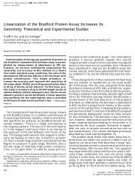
π (ϕ)<br />
0<br />
π x<br />
(ϕ)<br />
(ϕ *) σ−1 (ϕ x *) σ−1<br />
-f<br />
-f x<br />
ϕ σ−1<br />
Figure 2.1: Firm Behavior<br />
only if ϕ>ϕ ∗ .Thisimpliesthatafirm will rema<strong>in</strong> <strong>in</strong> the market and produce<br />
if and only if it is sufficiently productive. Follow<strong>in</strong>g Helpman, Melitz and Yeaple<br />
(2003) and Antràs and Helpman (2003), Figure 2.1 illustrates the equilibrium.<br />
Notice that profits are proportional to ϕ σ−1 ,andthatπ (0) = −f.<br />
• Consider next the <strong>in</strong>dustry equilibrium, where we solve for the endogenously<br />
determ<strong>in</strong>ed measure M of firms (and varieties), as well as for the distribution<br />
of (active firms’) productivities <strong>in</strong> the economy µ (ϕ). We follow Melitz (2003)<br />
<strong>in</strong> express<strong>in</strong>g all the equilibrium conditions <strong>in</strong> terms of the cutoff ϕ ∗ and then<br />
obta<strong>in</strong><strong>in</strong>g the rema<strong>in</strong><strong>in</strong>g variables of <strong>in</strong>terest from it. For that purpose, it is useful<br />
to start by def<strong>in</strong><strong>in</strong>g the weighted average productivity measure,<br />
∙Z ∞<br />
eϕ = ϕ σ−1 µ (ϕ) dϕ¸1/(σ−1)<br />
,<br />
0<br />
which, as we will see, completely summarizes the relevant <strong>in</strong>formation <strong>in</strong> the<br />
16
distribution of probabilities. Notice that the conditional distribution µ (ϕ) equals:<br />
µ (ϕ) =<br />
( g(ϕ)<br />
1−G(ϕ ∗ )<br />
if ϕ ≥ ϕ ∗<br />
0 otherwise ,<br />
from which<br />
∙ Z<br />
eϕ (ϕ ∗ 1 ∞<br />
¸1/(σ−1)<br />
)=<br />
ϕ σ−1 g (ϕ) dϕ , (2.8)<br />
1 − G (ϕ ∗ ) ϕ ∗<br />
and hence eϕ is uniquely p<strong>in</strong>ned down by ϕ ∗ and the exogenous (unconditional)<br />
distributions g (ϕ) and G (ϕ).<br />
Next, we can def<strong>in</strong>e average profits π = π (eϕ) as<br />
π = r (eϕ) µ Ã<br />
eϕ (ϕ ∗ σ−1 µ !<br />
σ − f = ) r (ϕ ∗ )<br />
eϕ (ϕ ∗ σ−1<br />
)<br />
− f = f<br />
− 1 , (ZCP)<br />
ϕ ∗ σ<br />
ϕ ∗ (2.9)<br />
where we have used (2.5), (2.6) and π (ϕ ∗ )=0. 2<br />
F<strong>in</strong>ally, free entry ensures that, <strong>in</strong> the <strong>in</strong>dustry equilibrium, the expected discounted<br />
value of profits for a potential entrant equal the fixed cost of entry, or 3<br />
Z ∞<br />
0<br />
v (ϕ) g (ϕ) dϕ = f e ⇔ π =<br />
δf e<br />
. (FE) (2.10)<br />
1 − G (ϕ ∗ )<br />
Notice that (2.9) and (2.10) form a system of two equations <strong>in</strong> two unknowns<br />
π and ϕ ∗ . Because G 0 (ϕ ∗ ) > 0, it is clear that along the FE schedule π is an<br />
<strong>in</strong>creas<strong>in</strong>g function of ϕ ∗ and satisfies π (0) = δf e and lim ϕ ∗ →∞ π (ϕ ∗ )=∞. Intuitively,<br />
for a given expected value of entry f e , the probability of success should<br />
be decreas<strong>in</strong>g <strong>in</strong> the average profit level π. Hence, an <strong>in</strong>crease <strong>in</strong> π should be<br />
matchedbyan<strong>in</strong>crease<strong>in</strong>ϕ ∗ . On the other hand, Melitz (2003) shows that<br />
the FE curve is cut by the ZCP curve only once from above, thus ensur<strong>in</strong>g the<br />
existence and uniqueness of the equilibrium. Furthermore, under common distributions,<br />
the ZCP schedule is downward slop<strong>in</strong>g <strong>in</strong> the space (π, ϕ ∗ ) (see Figure<br />
2 Notice that we refer to these as average profits because π = R ∞<br />
π (ϕ) µ (ϕ) dϕ (go ahead and<br />
0<br />
prove it!).<br />
3 Notice that R ∞<br />
R ∞<br />
π (ϕ) µ (ϕ) dϕ =<br />
ϕ ∗<br />
1<br />
δ [1 − G (ϕ∗ )] π.<br />
v (ϕ) g (ϕ) dϕ = R ∞ 1<br />
0 ϕ ∗ δ π (ϕ) g (ϕ) dϕ = [1− G (ϕ∗ )] 1 δ<br />
17
2.2 below). Intuitively, an <strong>in</strong>crease <strong>in</strong> ϕ ∗ will <strong>in</strong>crease the average productivity<br />
of the surviv<strong>in</strong>g firms<br />
eϕ (ϕ ∗ ) 0 =<br />
g (ϕ ∗ ) eϕ 2−σ<br />
(σ − 1) (1 − G (ϕ ∗ )) 2 Z ∞<br />
ϕ ∗ ¡<br />
ϕ σ−1 − (ϕ ∗ ) σ−1¢ g (ϕ) dϕ > 0.<br />
Because profits tend to <strong>in</strong>crease with a firm’s productivity, an <strong>in</strong>crease <strong>in</strong> ϕ ∗ will<br />
have a direct positive effect on profits π. But because firm profits are decreas<strong>in</strong>g<br />
<strong>in</strong> the productivity of rivals, there is also an additional effect that goes <strong>in</strong> the<br />
opposite direction. If the distribution G (ϕ) has a fat enough right tail, the latter<br />
effect will dom<strong>in</strong>ate and the ZCP will be downward slop<strong>in</strong>g. An <strong>in</strong>terest<strong>in</strong>g case<br />
³<br />
b<br />
is that of a Pareto distribution, i.e., G (ϕ) =1− ϕ´k,<br />
whichyields<br />
eϕ (ϕ ∗ ) =<br />
⎡<br />
⎢<br />
⎣³<br />
1<br />
´k<br />
b<br />
ϕ ∗<br />
µ k−1 b<br />
ϕ σ−1 ⎥<br />
kb dϕ⎦<br />
ϕ ϕ<br />
∗<br />
Z ∞<br />
⎤<br />
1/(σ−1)<br />
=<br />
=<br />
Z Ã !<br />
∞<br />
¸1/(σ−1) ∙k (ϕ ∗ ) k ϕ σ−k k (ϕ ∗ ) σ−1 1/(σ−1)<br />
dϕ = ,<br />
σ − k +1<br />
ϕ ∗<br />
and the ZCP schedule is flat.<br />
• Once we have the equilibrium values of ϕ ∗ and π, we can easily solve for the equilibrium<br />
number of firms. Notice that the identical price <strong>in</strong>dex <strong>in</strong> (2.2) becomes<br />
simply:<br />
P 1−σ =<br />
Z<br />
p (ω) 1−σ dω =<br />
∞Z<br />
(ρϕ) σ−1 Mµ(ϕ) dϕ = M (ρeϕ) σ−1 ,<br />
ω∈Ω<br />
0<br />
and hence,<br />
π = 1 R<br />
σ M − f.<br />
F<strong>in</strong>ally notice that the equality of <strong>in</strong>come and expenditure (R = L) implies that: 4<br />
M =<br />
L<br />
σ (π + f) , (2.11)<br />
4 In particular, R = Π + L p = Mπ + L p = δM<br />
1−G(ϕ ∗ ) f e + L p = M e f e + L p = L e + L p = L.<br />
18
which completes the characterization of the stationary equilibrium of the closed<br />
economy.<br />
• Notice the follow<strong>in</strong>g features of the equilibrium:<br />
— eϕ, ϕ ∗ , π and µ (ϕ) are <strong>in</strong>dependent of L, whileM is proportional to country<br />
size.<br />
— Welfareisgivenby<br />
⎛<br />
Z<br />
⎞1/ρ<br />
⎛<br />
Z<br />
U = ⎝ q (ω) ρ dω⎠<br />
= ⎝<br />
ω∈Ω<br />
ω∈Ω<br />
⎞<br />
µ<br />
ρ<br />
L<br />
M (ρeϕ) σ−1 (ρϕ)σ µ (ϕ) dϕ⎠<br />
— Notice that the aggregate outcome predicted by the model is identical to<br />
that generated by a Krugman (1980) model with homogenous firms with<br />
productivity eϕ. This shows how nicely the model aggregates the sectoral<br />
heterogeneity.<br />
1/ρ<br />
= LM 1/(σ−1) ρeϕ<br />
The Open Economy Model<br />
• With this mach<strong>in</strong>ery at hand, we can now move to the open economy version<br />
of the model and analyze the export<strong>in</strong>g decision as well as the reallocation effects<br />
generated by trade. If trade open<strong>in</strong>g is just an <strong>in</strong>crease <strong>in</strong> the relevant size of the<br />
economy, then we know that all firms will export and also, from the equilibrium<br />
above, that trade will have no impact on average productivity (see, however,<br />
footnote 16 as well as Melitz and Ottaviano, 2003, for the importance of CES<br />
preferences for these results). Melitz (2003) thus <strong>in</strong>troduces trade frictions. These<br />
are of two types:<br />
1. A standard per-unit iceberg costs, so that τ units need to be shipped for 1<br />
unit to make it to any foreign country;<br />
2. An <strong>in</strong>itial fixed cost of f ex units of labor to start export<strong>in</strong>g, which is <strong>in</strong>curred<br />
once the firm has learned ϕ.<br />
19
It is also assumed that the domestic economy can trade with n ≥ 1 other countries<br />
and that all countries are of equal size, which implies that factor price equalization<br />
will hold and the wage will equal 1 everywhere.<br />
• Let us consider the implications of this extended set-up for firm behavior. It<br />
is well-known (remember Chapter 1!) that the iceberg transport cost does not<br />
affect the elasticity of demand faced by each producer. It follows that firms will<br />
aga<strong>in</strong> charge a constant markup over marg<strong>in</strong>al cost, but notice that the latter<br />
will be higher for exports. Notice that, as <strong>in</strong> the closed economy, revenues from<br />
domestic sales are:<br />
r d (ϕ) =R (Pρϕ) σ−1<br />
where as revenues from foreign sales <strong>in</strong> country k are:<br />
r x (ϕ) =τ 1−σ R k (P k ρϕ) σ−1 .<br />
As we will see later, the assumption of factor price equalization will imply that<br />
RP σ−1 = R k P σ−1<br />
k<br />
for all k, so follow<strong>in</strong>g Melitz we can express firm revenues by<br />
export status as<br />
r (ϕ) =<br />
(<br />
r d (ϕ)<br />
if the firm does not export<br />
(1 + nτ 1−σ ) r d (ϕ) if the firm exports to all countries.<br />
As before, profits from domestic sales are simply<br />
π d (ϕ) = r d (ϕ)<br />
σ<br />
− f, (2.12)<br />
while profits from export<strong>in</strong>g to a particular country are given by<br />
π x (ϕ) = r x (ϕ)<br />
σ<br />
− f x = τ 1−σ r d (ϕ)<br />
σ<br />
− f x , (2.13)<br />
where f x is amortized per-period portion of the <strong>in</strong>itial fixed cost (i.e., δf ex ). 5<br />
Notice that eq. (2.13) is <strong>in</strong>dependent of the import<strong>in</strong>g country k, and hence a<br />
5 Remember that we focus on stationary equilibrium and that the sunk cost of export<strong>in</strong>g is <strong>in</strong>curred<br />
after ϕ has been revealed. Hence, the firmwilleithernotexportorexport<strong>in</strong>everyperiod.<br />
20
firm does not export at all or it exports to all countries. Per period profits are<br />
therefore π (ϕ) =π d (ϕ)+max{0,nπ x (ϕ)} while the present discounted value of<br />
profits is given by aga<strong>in</strong> by (2.7), i.e., v (ϕ) =max{0,π(ϕ) /δ}. Thisnowdef<strong>in</strong>es<br />
two thresholds:<br />
ϕ ∗ =<strong>in</strong>f{ϕ : v (ϕ) > 0}<br />
and<br />
ϕ ∗ x =<strong>in</strong>f{ϕ : ϕ ≥ ϕ ∗ and π x (ϕ) > 0} .<br />
Importantly, because RP σ−1 is identical <strong>in</strong> all country, ϕ ∗ will also be identical<br />
everywhere. Notice that firms with ϕ ≥ ϕ ∗ will rema<strong>in</strong> <strong>in</strong> the market after<br />
learn<strong>in</strong>g their productivity, while those with ϕ ≥ ϕ ∗ x will not only produce domestically,<br />
but also export. So long as ϕ ∗ x >ϕ ∗ the model is able to replicate<br />
the micro-level f<strong>in</strong>d<strong>in</strong>gs that the more productive firmswith<strong>in</strong>an<strong>in</strong>dustryselfselect<br />
<strong>in</strong>to the export market. This will hold true whenever τ σ−1 f x >f, a case<br />
illustrated <strong>in</strong> Figure 2.1.<br />
• Important: It is clear that <strong>in</strong> the model, a higher ϕ is associated with a higher<br />
productivity level. But is it also associated with a higher measured productivity<br />
level? In Chapter 1, we saw that the evidence <strong>in</strong>dicates that exporters feature a<br />
higher value added per worker. One is tempted to identify this with the firm’s<br />
mark-up, which <strong>in</strong> Melitz’s (2003) model is <strong>in</strong>dependent of ϕ. His model would<br />
then not be able to account for heterogeneity <strong>in</strong> measured productivity. But, <strong>in</strong><br />
fact, tak<strong>in</strong>g account of the fixedcosts,onecaneasilyshowthat:<br />
r d (ϕ)+nr x (ϕ)<br />
q d (ϕ) /ϕ + nτq x (ϕ) /ϕ + f + f x<br />
><br />
r d (ϕ)<br />
q d (ϕ) /ϕ + f if and only if τ σ−1 f x >f,<br />
and hence the model is consistent with the evidence that uses the available measures<br />
of productivity. Notice that fixed costs are crucial for this. An alternative<br />
route explored by Bernard et al. (2003) is to dispense with fixed costs but <strong>in</strong>troduce<br />
a theory that generates variable markups. We will study this alternative<br />
approach <strong>in</strong> Chapter 3.<br />
• We next solve for the <strong>in</strong>dustry equilibrium to prepare the ground for the study of<br />
21
how the model can account for the type of trade-<strong>in</strong>duced reallocations stressed<br />
by the empirical literature. We are aga<strong>in</strong> go<strong>in</strong>g to follow Melitz’s approach of express<strong>in</strong>g<br />
all the relevant equilibrium conditions <strong>in</strong> terms of the cut-off ϕ ∗ .Forthat<br />
purpose, notice first that from (2.5), (2.13) and the def<strong>in</strong>ition of these thresholds,<br />
0= τ 1−σ r d (ϕ ∗ x)<br />
σ<br />
− f x = τ 1−σ (ϕ ∗ x) σ−1<br />
σ<br />
r (ϕ ∗ )<br />
(ϕ ∗ ) σ−1 − f x = τ 1−σ (ϕ ∗ x) σ−1<br />
(ϕ ∗ ) σ−1 f − f x<br />
or<br />
µ 1/(σ−1)<br />
ϕ ∗ x = ϕ ∗ fx<br />
τ<br />
.<br />
f<br />
The equilibrium distribution of productivity levels for <strong>in</strong>cumbent firms µ (ϕ) is<br />
aga<strong>in</strong> given by µ (ϕ) =g (ϕ) / [1 − G (ϕ ∗ )] for ϕ ≥ ϕ ∗ , while the probability that<br />
a surviv<strong>in</strong>g firm exports is given by p x =[1− G (ϕ ∗ x)] / [1 − G (ϕ ∗ )]. Next,wecan<br />
def<strong>in</strong>e eϕ (ϕ ∗ ) and eϕ x (ϕ ∗ x) as <strong>in</strong> (2.8), and aga<strong>in</strong> us<strong>in</strong>g the same type of weighted<br />
average to def<strong>in</strong>e<br />
eϕ t =<br />
½ 1 £ ¤ ¾ 1/(σ−1)<br />
M eϕ σ−1 + nM x τ 1−σ eϕ σ−1<br />
x<br />
M t<br />
(2.14)<br />
where M is the measure of domestic producers, nM x is the measure of foreign<br />
firms that sell <strong>in</strong> the domestic country, and M t = M + nM x . eϕ t is the average<br />
productivity of all firms compet<strong>in</strong>g <strong>in</strong> a country. As was the case <strong>in</strong> the closed<br />
economy, the aggregates R and P can be expressed <strong>in</strong> terms of eϕ t . Notice the<br />
importance of the symmetry assumption, which will ensure that the cutoff ϕ ∗ ,as<br />
well as M and M x , are identical for all countries, which <strong>in</strong> turn implies that eϕ t<br />
is also identical across countries.<br />
22
Next, we can def<strong>in</strong>e average expected profits as 6<br />
π = π d (eϕ)+p x nπ x (eϕ x )=<br />
à µ !<br />
eϕ (ϕ ∗ σ−1<br />
)<br />
= f<br />
− 1<br />
ϕ ∗<br />
which is the open-economy analog to (2.9).<br />
à µ eϕx (ϕ ∗ σ−1<br />
)<br />
+ p x nf x − 1!<br />
, (ZCP<br />
ϕ ∗ x (ϕ ∗ )<br />
t<br />
)(2.15)<br />
F<strong>in</strong>ally, the free entry condition requires the expected operat<strong>in</strong>g profits for a<br />
potential entrant to equal the sunk entry cost<br />
Z ∞<br />
0<br />
v (ϕ) g (ϕ) dϕ = f e ⇔ π =<br />
δf e<br />
1 − G (ϕ ∗ ) , (FE t ) (2.16)<br />
and hence this relationship rema<strong>in</strong>s unaltered <strong>in</strong> the open economy. We aga<strong>in</strong><br />
have a system of two equations <strong>in</strong> two unknowns π and ϕ ∗ ,whichweplot<strong>in</strong><br />
Figure 2.2.<br />
To solve for the equilibrium number of firms M, M x and M t notice that the M<br />
domestic producers together collect a revenue equal to R, while their average<br />
revenueisgivenby<br />
6 To see this note:<br />
π =<br />
=<br />
Z ∞<br />
0<br />
Z ∞<br />
0<br />
r =<br />
π (ϕ) µ (ϕ) dϕ =<br />
Z ∞<br />
³<br />
´<br />
R (Pρϕ) σ−1 − f µ (ϕ) dϕ + n<br />
0<br />
r (ϕ) µ (ϕ) dϕ = σ (π + f + p x nf x )<br />
à Z !<br />
∞<br />
Rτ 1−σ (Pρϕ) σ−1 − f x µ (ϕ) dϕ =<br />
Z ∞<br />
Z ∞<br />
= R (Pρ) σ−1 eϕ σ−1 − f + nRτ 1−σ (Pρ) σ−1 ϕ σ−1 µ (ϕ) dϕ − nf x µ (ϕ) dϕ =<br />
Z ∞<br />
= π d (eϕ)+nRτ 1−σ (Pρ) σ−1 ϕ σ−1 g (ϕ)<br />
ϕ 1 − G (ϕ ∗ ) dϕ − nf x<br />
∗ x<br />
ϕ ∗ x<br />
= π d (eϕ)+nRτ 1−σ (Pρ) σ−1 1 − G (ϕ ∗ x)<br />
1 − G (ϕ ∗ ) eϕσ−1 x − 1 − G (ϕ∗ x)<br />
1 − G (ϕ ∗ ) nf x<br />
= π d (eϕ)+p x nπ x (eϕ x )<br />
ϕ ∗ x<br />
ϕ ∗ x<br />
Z ∞<br />
ϕ ∗ x<br />
g (ϕ)<br />
1 − G (ϕ ∗ ) dϕ =<br />
23
and thus, impos<strong>in</strong>g the equality of <strong>in</strong>come and spend<strong>in</strong>g, we get<br />
M = R r =<br />
L<br />
σ (π + f + p x nf x )<br />
(2.17)<br />
and M t =(1+np x ) M. 7 This completes the characterization of the stationary<br />
equilibrium of the open economy.<br />
The Impact of Trade<br />
• Let’s follow Melitz and analyze the impact of trade by compar<strong>in</strong>g the stationary<br />
equilibria of the closed and open economy. Let ϕ ∗ a and eϕ a denote the cut-off and<br />
average productivities under autarky (as computed <strong>in</strong> the closed-economy model).<br />
From simple <strong>in</strong>spection of (2.9) and (2.15), it follows that the ZCP schedule <strong>in</strong><br />
the open economy is an upward shift of the ZCP schedule under autarky. It<br />
thus follows that ϕ ∗ >ϕ ∗ a and eϕ >eϕ a , as illustrated <strong>in</strong> Figure 2.2. Firms with<br />
productivity between ϕ ∗ a and ϕ ∗ are not able to earn positive operat<strong>in</strong>g profits<br />
under trade. Consistently with the f<strong>in</strong>d<strong>in</strong>gs <strong>in</strong> the empirical literature, exposure<br />
to trade thus forces the least productive firms to exit or shut-down (see Chapter<br />
1 and Chapter 4 later on).<br />
• It is important to understand the <strong>in</strong>tuition for this result. Remember that the<br />
elasticity of demand is unaffected by trade open<strong>in</strong>g, so the fall <strong>in</strong> profit for domestic<br />
producers is not expla<strong>in</strong>ed by a fall <strong>in</strong> mark-ups driven by <strong>in</strong>creased foreign<br />
competition. 8 The actual channel operates through the domestic factor market.<br />
In particular, trade translates <strong>in</strong>to <strong>in</strong>creased profitable opportunities for the rel-<br />
7 Notice also that the ideal price <strong>in</strong>dex can also be computed as follows:<br />
Z<br />
∞Z<br />
P 1−σ = p (ω) 1−σ dω = (ρϕ) σ−1 Mµ(ϕ) dϕ +<br />
Z ∞<br />
ϕ ∗ x<br />
ω∈Ω<br />
0<br />
= M (ρeϕ) σ−1 + nM x τ 1−σ (ρeϕ x ) σ−1 = M t (ρeϕ t ) σ−1 .<br />
τ 1−σ (ρϕ) σ−1 nM x µ (ϕ) dϕ =<br />
8 Depart<strong>in</strong>g from the CES preferences assumption, Melitz and Ottaviano (2003) develop a model<br />
<strong>in</strong> which trade liberalization leads to an <strong>in</strong>crease <strong>in</strong> the toughness of competition and an associated<br />
fall <strong>in</strong> markups. We will not go <strong>in</strong>to the details of this paper, but this should be required read<strong>in</strong>g for<br />
anyone <strong>in</strong>terested <strong>in</strong> this area.<br />
24
π<br />
(FE)<br />
π<br />
π a<br />
δf e<br />
(ZCP)<br />
(Trade)<br />
(Autarky)<br />
∗<br />
ϕ a<br />
∗<br />
ϕ<br />
ϕ<br />
Figure 2.2: The Impact of Trade on the Industry Equilibrium<br />
atively productive firms that can afford the fixed export<strong>in</strong>g cost. This translates<br />
<strong>in</strong>to more entry, thereby <strong>in</strong>creas<strong>in</strong>g labor demand and (given the fixed supply of<br />
labor) lead<strong>in</strong>g to a rise <strong>in</strong> the real wage (w/P). This, <strong>in</strong> turn, br<strong>in</strong>gs down the<br />
profit level of the least productive firmstoalevelthatforcesthemtoexit.<br />
• Notice also that π>π a , which from (2.11) and (2.17), implies that MM a . And even when this does not hold, Melitz shows that<br />
welfare unambiguously goes up (due to aggregate productivity ga<strong>in</strong>, see p. A-3).<br />
• F<strong>in</strong>ally, we are <strong>in</strong>terested <strong>in</strong> show<strong>in</strong>g that the model can replicate the type of<br />
market shares reallocations found <strong>in</strong> the data. In particular, we want to show<br />
that:<br />
r d (ϕ)
which proves the first <strong>in</strong>equality. The second <strong>in</strong>equality is more cumbersome to<br />
establish as its proof requires an analysis of the elasticity of the equilibrium ϕ ∗<br />
with respect to τ (see Appendix E <strong>in</strong> the paper for details).<br />
• Melitz also describes the effects on firm profits and shows that the most efficient<br />
firms are those that stand to ga<strong>in</strong> the most from exposure to trade, while a<br />
range of exporters see their profits squeeze <strong>in</strong> spite of the <strong>in</strong>creased market share<br />
(export<strong>in</strong>g br<strong>in</strong>gs positive profitsbutnotlargeenoughtocompensatefortheloss<br />
<strong>in</strong> profits from domestic sales and the fixed cost of export<strong>in</strong>g).<br />
• In the last section, Melitz demonstrates that similar reallocation effects arise <strong>in</strong><br />
response to smooth variations <strong>in</strong> τ and n. This is important because there is<br />
some tension between the previous comparison of steady states equilibria (which<br />
captures long-run consequences of trade) and the type of short-run adjustments<br />
unveiled by the empirical literature. The added appeal of these smooth comparative<br />
statics comes at the cost of substantially more cumbersome algebra.<br />
26
Chapter 3<br />
Intra<strong>in</strong>dustry Heterogeneity and<br />
Bertrand Competition: Bernard,<br />
Eaton, Jensen, and Kortum (2003)<br />
• Bernard et al. (hereafter, BEJK) develop an alternative model of firm heterogeneity<br />
along the l<strong>in</strong>es of the probabilistic model of comparative advantage of<br />
Eaton and Kortum (Econometrica, 2002). Because the firm-level facts that motivate<br />
the paper have been discussed <strong>in</strong> Chapter 1, I focus here on their theoretical<br />
framework and simulation results.<br />
Set-up<br />
• On the demand side, preferences are symmetric across goods, CES and identical<br />
<strong>in</strong> all N countries, but unlike <strong>in</strong> Melitz (2003), the measure of goods is fixed at<br />
one. Follow<strong>in</strong>g their notation, expenditure on good j <strong>in</strong> country n is given by<br />
X n (j) =x n<br />
µ<br />
Pn (j)<br />
p n<br />
1−σ<br />
,<br />
where P n (j) is the price of good j <strong>in</strong> country n, x n is total expenditure <strong>in</strong> n and<br />
p n is the ideal price <strong>in</strong>dex<br />
∙Z 1<br />
p n = P n (j) dj¸1/(1−σ) 1−σ .<br />
0<br />
27
Notice that unlike Melitz (2003), lower case letters denote aggregates, while upper<br />
case letters refer to good-specific variables.<br />
• On the supply side, each country has multiple potential producers of good<br />
j with vary<strong>in</strong>g levels of technical efficiency. As <strong>in</strong> Melitz (2003), productivity<br />
heterogeneity is driven by differences <strong>in</strong> the marg<strong>in</strong>al cost of production. The<br />
kth most efficient producer of good j <strong>in</strong> country i needs to hire 1/Z ki (j) units<br />
of the unique composite factor of production (e.g., workers) to produce one unit<br />
of the good. There are no fixed costs of production so the technology features<br />
constant returns to scale.<br />
All goods are tradable but d ni ≥ 1 units of the good need to be shipped from<br />
country i for 1 unittomaketocountryn. It is assumed that d ni = 1 and<br />
that d ni ≤ d nk d ki .Noticethatthefirst (second) letter of subscripts denotes the<br />
dest<strong>in</strong>ation (orig<strong>in</strong>) country.<br />
The composite <strong>in</strong>put is perfectly mobile with<strong>in</strong> countries, but not between them.<br />
The cost of such <strong>in</strong>put will therefore generally vary across countries (remember<br />
that <strong>in</strong> Melitz’s model countries were identical), and will be denoted by w i .<br />
From the previous assumptions, it follows that the kth most efficient producer of<br />
good j can deliver the good <strong>in</strong> country i at unit cost:<br />
C kni (j) =<br />
w i<br />
Z ki (j) d ni (3.1)<br />
• It is assumed that potential sellers <strong>in</strong> country n compete à la Bertrand. As with<br />
perfect competition, the most efficient (lowest-price) firm captures the market<br />
and becomes the only seller <strong>in</strong> n, but with productivity heterogeneity, the price<br />
it can charge will generally be above marg<strong>in</strong>al cost. In particular, this optimal<br />
price is<br />
P n (j) =m<strong>in</strong>{C 2n (j) , mC 1n (j)} ,<br />
28
where<br />
½<br />
¾<br />
C 1n (j) =m<strong>in</strong>{C 1ni (j)} = C 1ni ∗ (j) ≤ m<strong>in</strong><br />
i<br />
C 2ni ∗ (j) , m<strong>in</strong> i6=i ∗ 1ni (j)} = C 2n (j)<br />
(3.2)<br />
and<br />
(<br />
σ/ (σ − 1)<br />
m =<br />
∞<br />
if σ>1<br />
otherwise .<br />
Notice that P n (j) =C 2n (j) is more likely the higher the ratio C 2n (j) /C 1n (j)<br />
and the lower the elasticity of substitution σ. Ifthisisthecase,themarkupwill<br />
be a function of C 2n (j) /C 1n (j).<br />
From equations (3.1) and (3.2), it is clear that C 2n (j) /C 1n (j) will depend on<br />
the ratio of these two producers Z’s and, when i 6= i ∗ <strong>in</strong> eq. (3.2), it will also<br />
depend on relative <strong>in</strong>put costs and transport costs.<br />
• Follow<strong>in</strong>g Eaton and Kortum (2002), BEJK next adopt a probabilistic representation<br />
of the relevant efficiency parameters Z 1i (j) and Z 2i (j). This is a very<br />
useful trick because it allows to derive implications for trade flows <strong>in</strong> terms of<br />
the small number of parameters that characterize the underly<strong>in</strong>g probability distribution<br />
from which the efficiency parameters are drawn. Notice that is similar<br />
<strong>in</strong> spirit to Melitz’s approach, but the BEJK approach is more general <strong>in</strong> certa<strong>in</strong><br />
aspects (for <strong>in</strong>stance, countries are asymmetric and so are the probability<br />
distributions from which the Z’s are drawn).<br />
On the other hand, the BEJK approach is a bit less general <strong>in</strong> that they focus<br />
on a particularly convenient probability distribution. In particular, they assume<br />
that for a particular country i, the jo<strong>in</strong>t distribution of Z 1i (j) and Z 2i (j) takes<br />
the generalized Fréchet form<br />
F i (z 1 ,z 2 )=Pr[Z 1i
— θ>1 measures the amount of variability <strong>in</strong> the distribution. A lower θ<br />
implies more variability and thus will strengthen the potential ga<strong>in</strong>s from<br />
comparative advantage.<br />
— The distribution F i (z 1 ,z 2 ) is <strong>in</strong>dependent of j and of i 0 6= i. This means<br />
that unlike <strong>in</strong> the classical Ricardian world, here countries are not <strong>in</strong>herently<br />
better at produc<strong>in</strong>g particular types of goods. Actual comparative advantage<br />
is here stochastic.<br />
The Beauty of the Fréchet Distribution<br />
• We will see below that the model is able to account for several stylized facts<br />
emphasized <strong>in</strong> the literature on export<strong>in</strong>g and productivity, which we mentioned<br />
<strong>in</strong> Chapter 1 and will review at greater length <strong>in</strong> Chapter 4. Although for some of<br />
the results below the Fréchet assumption is actually unnecessary, some derivations<br />
below do require that we first spend some time discuss<strong>in</strong>g a few properties of the<br />
equilibrium distributions of costs and markups across countries.<br />
• Let us compute first the implied jo<strong>in</strong>t distribution of the lowest cost C 1n and<br />
second-lowest cost C 2n of supply<strong>in</strong>g some good to country n. It is worth follow<strong>in</strong>g<br />
the proof step by step (the details are not <strong>in</strong> the paper, but can be found <strong>in</strong> their<br />
Mathematical Appendix, which I closely follow). First, for a dest<strong>in</strong>ation country<br />
n and orig<strong>in</strong> country i, notice that for c 2 ≥ c 1 ,<br />
∙<br />
G c ni(c 1 ,c 2 ) = Pr[C 1ni ≥ c 1 ,C 2ni ≥ c 2 ]=Pr Z 1i ≤ w id ni<br />
,Z 2i ≤ w ¸<br />
id ni<br />
=<br />
c 1 c<br />
" Ã 2<br />
= F i ( w id ni<br />
, w µwi −θ µ !# −θ <br />
id ni<br />
d ni wi d ni<br />
)= 1+T i −<br />
e −T wi d −θ ni<br />
i c 2 =<br />
c 1 c 2 c 2<br />
c 1<br />
h<br />
= 1+T i (w i d ni ) −θ ¡ c θ 2 − c1¢ i θ e −T i(w i d ni ) −θ c θ 2<br />
(3.4)<br />
30
Next, from the def<strong>in</strong>itions <strong>in</strong> (3.1), as well as from (3.3) and (3.4),<br />
G c n(c 1 ,c 2 ) = Pr[C 1n ≥ c 1 ,C 2n ≥ c 2 ]=<br />
=<br />
NY<br />
NX<br />
G c ni (c 2 ,c 2 )<br />
=<br />
+<br />
i=1<br />
i=1<br />
C 1ni ≥c 2 & C 2ni ≥c 2<br />
| {z }<br />
Prob all countries have<br />
i=1<br />
i=1<br />
[G c ni (c 1 ,c 2 ) − G c ni (c 2 ,c 2 )]<br />
| {z } ×<br />
Extra Prob C 1n ≥c 1 (remember c 2 >c 1 )<br />
NY<br />
G c nk (c 2 ,c 2 )<br />
=<br />
k6=i<br />
| {z }<br />
Prob k6=i still have<br />
C 1nk ≥c 2 & C 2nk ≥c 2<br />
NY<br />
X N h<br />
e −T i(w i d ni ) −θ c θ 2 + T i (w i d ni ) −θ ¡ i Y N<br />
c θ 2 − c1¢ θ e<br />
−T i (w i d ni ) −θ c θ 2<br />
= e −Φ nc θ 2 + e<br />
−Φ n<br />
¡<br />
c θ 2 c<br />
θ<br />
2 − c θ 1<br />
¢<br />
Φn<br />
k6=i<br />
e −T k(w k d nk ) −θ c θ 2 =<br />
where,<br />
F<strong>in</strong>ally,<br />
Φ n =<br />
NX<br />
T i (w i d ni ) −θ .<br />
i=1<br />
G n (c 1 ,c 2 ) = Pr[C 1n ≤ c 1 ,C 2n ≤ c 2 ]=<br />
= 1− G c n (0,c 2 ) − G c n (c 1 ,c 1 )+G c n (c 1 ,c 2 )=<br />
= 1− e −Φ nc θ 1 − Φn c θ 1e −Φ nc θ 2 . (3.5)<br />
The simple form of (3.5) illustrates the usefulness of the Fréchet distribution<br />
<strong>in</strong> characteriz<strong>in</strong>g the jo<strong>in</strong>t distribution of extreme values, such as C 1n and C 2n<br />
(the same of course is true <strong>in</strong> a univariate set up, such as <strong>in</strong> Eaton and Kortum,<br />
2002). Furthermore, as <strong>in</strong> Melitz (2003), the choice of functional forms permits an<br />
elegant aggregation of the <strong>in</strong>herent heterogeneity <strong>in</strong> these models. In particular,<br />
Φ n captures all the relevant <strong>in</strong>formation on the efficiency distributions, <strong>in</strong>put<br />
costs, and trade costs around the world, and the jo<strong>in</strong>t distribution of c 1 and c 2 is<br />
<strong>in</strong>dependent of the actual sources of supply to country n.<br />
• In the derivations below, we will also make use of the follow<strong>in</strong>g results, which are<br />
relatively easy to derive us<strong>in</strong>g the jo<strong>in</strong>t cdf <strong>in</strong> eq. (3.5) (see their Mathematical<br />
Appendix for details).<br />
31
— The marg<strong>in</strong>als distribution of the lowest cost and second lowest suppliers to<br />
country n are given by:<br />
G 1n (c 1 ) = lim<br />
c 2 →∞ G n(c 1 ,c 2 )=1− e −Φncθ 1 ,<br />
and<br />
G 2n (c 2 )= lim G n (c 1 ,c 2 )=1− ¡ ¢<br />
1+Φ n c θ 2 e<br />
−Φ n c θ 2 .<br />
c 1 →c 2<br />
— The markup of the unique seller <strong>in</strong> country n is the realization of a random<br />
variable M n drawn from a Pareto distribution truncated at m. Toseethis<br />
def<strong>in</strong>e Mn 0 = C 2n /C 1n so that M n =m<strong>in</strong>{Mn, 0 m}. Noticefirst that:<br />
Pr [Mn 0 ≤ m 0 |C 2n = c 2 ] = Pr[c 2 /m 0 ≤ C 1n
perworkerofafirm sell<strong>in</strong>g <strong>in</strong> country n from country i ∗ is given by:<br />
P n (j) Q n (j)<br />
Q n (j) C 1n (j) /w i ∗<br />
= M n (j) w i ∗<br />
It easy to see that the model implies that, on average, plants that are more<br />
efficient charge a higher markup. In particular, conditional on a productivity<br />
level z 1 , the distribution of the markup is: 1<br />
H n (m|z 1 )=Pr[M n ≤ m|Z 1n = z 1 ]=<br />
(<br />
1 − e −Φ nw n z −θ<br />
1 (m θ −1)<br />
1 ≤ mϕ ∗ .Inwords,only a fraction<br />
of those that sell at home will also export abroad. Thisissimplyexpla<strong>in</strong>edby<br />
the fact that, because of transports costs, export<strong>in</strong>g anywhere imposes a higher<br />
efficiency hurdle than sell<strong>in</strong>g only at home. Notice that this is <strong>in</strong>dependent<br />
of the Fréchet assumption. The crucial features of the model for this result<br />
1 This follows from,<br />
and C 1n =<br />
Pr [M 0 n ≤ m 0 |C 1n = C 1 ]=<br />
R m 0 c 1<br />
c 1<br />
³<br />
dGn (c 1 ,c 2 )<br />
dc 1 dc 2<br />
´<br />
dc 2<br />
dG 1n (c 1 ) /dc 1<br />
=1− e −Φncθ 1(m 0θ −1) ,<br />
w n<br />
Z 1n (j) (the efficiency Z 1n (j) is <strong>in</strong>clusive of the transport cost).<br />
33
are that (i) it is too costly for firms to differentiate their products and that (ii)<br />
potential producers of a good compete <strong>in</strong> prices, thus lead<strong>in</strong>g to sales by only the<br />
lowest-cost deliverer <strong>in</strong> a given country.<br />
Furthermore, the assumption that the Fréchet distribution is <strong>in</strong>dependent of j,<br />
also implies that export<strong>in</strong>g firms <strong>in</strong> a given country will, on average, appear<br />
to be more productive than firms that sell only domestically.<br />
3. Size: The distribution of the second-lowest cost, which if M n < m determ<strong>in</strong>es<br />
the price, conditional on the lowest cost is given by:<br />
Pr [C 2n ≤ c 2 |C 1n = c 1 ]=<br />
R c2<br />
c 1<br />
³<br />
dGn(c 1 ,c 2 )<br />
dc 1 dc 2<br />
´<br />
dc 2<br />
dG 1n (c 1 ) /dc 1<br />
= dG n(c 1 ,c 2 )/dc 1<br />
dG 1n (c 1 ) /dc 1<br />
=1−e −Φ n(c θ 2 −cθ 1) ,<br />
and is therefore stochastically <strong>in</strong>creas<strong>in</strong>g <strong>in</strong> c 1 —rememberthatF (x) first order<br />
stochastically dom<strong>in</strong>ates G (x) if and only F (x) 1, it follows that exporters will on<br />
averagebebigger(have higher domestic sales) than non-exporters. 2<br />
One might f<strong>in</strong>d confus<strong>in</strong>g that, on the one hand, exporters tend to charge relatively<br />
high markups, whereas, on the other hand, they tend to charge relatively<br />
low prices. Notice, however, that this just reflects that the lower is C 1n (i.e., the<br />
more efficient is the least-cost producer), the lower is C 2n also (and hence the<br />
lower is the price), but the higher is C 2n /C 1n (and thus the higher is the markup).<br />
Quantification and Counterfactuals<br />
• As we have just seen, the model is able to qualitatively replicate some of the<br />
f<strong>in</strong>d<strong>in</strong>gs <strong>in</strong> the empirical literature on productivity and export<strong>in</strong>g. BEJK next<br />
2 This discussion has presumed M n < m, but it is straightforward to show that the same is true<br />
when M n = m.<br />
34
explore whether the model also does a good quantitative job. For this purpose,<br />
the authors first show that simulat<strong>in</strong>g the model only requires data on bilateral<br />
trade shares π ni between any two countries, total consumption (or absorption)<br />
x n for each country n, aswellasvaluesfortheparametersσ and θ. 3<br />
Def<strong>in</strong><strong>in</strong>g the transformations<br />
U 1i (j) = T i Z 1i (j) −θ<br />
U 2i (j) = T i Z 2i (j) −θ ,<br />
one can show that U 1i (j) and U 2i (j) are random variables drawn from a parameterfree<br />
distribution characterized by:<br />
Pr [U 1i (j) ≤ u 1 ] = 1− e −u 1<br />
Pr [U 2i (j) ≤ u 2 |U 1i (j) =u 1 ] = 1− e −u 2+u 1<br />
. (3.6)<br />
The authors then implement the follow<strong>in</strong>g algorithm (see paper for more details):<br />
1. They draw U 1i (j) and U 2i (j) from (3.6) for 47 countries and 1,000,000 goods<br />
j.<br />
2. For each dest<strong>in</strong>ation country n and good j, they identify the source country<br />
i ∗ from:<br />
½ ¾<br />
i ∗ U1i (j)<br />
=argm<strong>in</strong> ,<br />
i<br />
where π ni is the ratio of i’s exports to n divided by n 0 s total absorption.<br />
3. Lett<strong>in</strong>g i ∗ = USA and identify<strong>in</strong>g a good j with a plant, this delivers a<br />
simulated sample of active U.S. active plants and their export status.<br />
4. For each plant j, <strong>in</strong>formation on U 1i (j) and U 2i (j) (as well as π ni for all i)<br />
is sufficient to compute the markup charged <strong>in</strong> country n, fromwhichsales,<br />
exports, andtotal production costs can easily be computed (see eq. 16<br />
and 17 <strong>in</strong> their paper).<br />
3 In particular, data on the other parameters of the model w i , T i and d ni are not needed.<br />
π ni<br />
35
5. F<strong>in</strong>ally, assum<strong>in</strong>g that the composite factor of production is a Cobb-Douglas<br />
aggregator of wages and <strong>in</strong>termediate <strong>in</strong>puts (which are themselves an aggregate<br />
of all the j’s), permits computation of employment and value<br />
added per worker.<br />
• The procedure is repeated for different values of σ and θ search<strong>in</strong>g for the valuesthatdeliverthesameproductivityadvantageofexporters(rememberfrom<br />
Chapter 1 that their value added per worker is 33% higher) and the same size<br />
advantage (on average, exporters ship domestically 4.8 times more than nonexporters).<br />
This yields σ =3.79 and θ =3.60.<br />
With these parameter values, it is assessed how well the model fits the other<br />
facts regard<strong>in</strong>g export<strong>in</strong>g and productivity. The model does a pretty good job<br />
and <strong>in</strong> particular the simulations match the skewness of the distribution of export<br />
<strong>in</strong>tensity, with most exporters sell<strong>in</strong>g only a small fraction of their output abroad.<br />
Nevertheless, the model tends to overpredict the fraction of firm that export and<br />
underpredict the variability <strong>in</strong> productivity and <strong>in</strong> size.<br />
• The f<strong>in</strong>al section of the paper performs a couple of counterfactual experiments:<br />
(i)a5%worldwidedecl<strong>in</strong>e<strong>in</strong>tradecosts,and(ii)a10%<strong>in</strong>crease<strong>in</strong>U.S.wages<br />
(U.S. dollar real appreciation). The results of (i) <strong>in</strong>dicate that the model is also<br />
able to replicate the positive aggregate productivity effects of trade liberalization<br />
documented by Pavcnik (2002) and others. In particular, as <strong>in</strong> Melitz (2003),<br />
the model features reallocation effects by which the fall <strong>in</strong> trade costs leads to<br />
exit of relatively unproductive domestic producers and expansion of relatively<br />
productive exporters. 4 Unlike <strong>in</strong> Melitz (2003), however, the model also generates<br />
substantial productivity ga<strong>in</strong>s with<strong>in</strong> surviv<strong>in</strong>g firmsdrivenbythedecl<strong>in</strong>e<strong>in</strong>the<br />
price of <strong>in</strong>termediate <strong>in</strong>puts.<br />
Limitations and Extensions<br />
• An implication of the framework is that the number of country i’s exporters<br />
4 Remember, however that the mechanism is different. Here, exit is a direct consequence of <strong>in</strong>tensified<br />
price competition from foreign suppliers.<br />
36
to country n should vary proportionately with the market share of country i <strong>in</strong><br />
country n’s imports. Eaton, Kortum and Kramarz (2003) show that this feature is<br />
not borne by data on French firms. In particular, they f<strong>in</strong>d that for a given level of<br />
French market share <strong>in</strong> country n, the number of exporters is significantly higher,<br />
the higher country n’s market share. To account for this <strong>in</strong>terest<strong>in</strong>g f<strong>in</strong>d<strong>in</strong>g, they<br />
modify the BEJK set-up by <strong>in</strong>clud<strong>in</strong>g fixed costs of export<strong>in</strong>g as well as Cournot<br />
competition.<br />
37
Chapter 4<br />
Firms and the Decision to Export:<br />
Empirics<br />
• In this chapter, we will first briefly discuss a few recent empirical studies on<br />
the l<strong>in</strong>k between export<strong>in</strong>g and plant-level performance. We will then study<br />
<strong>in</strong> more depth a particularly <strong>in</strong>terest<strong>in</strong>g recent paper by Pavcnik (2002) on the<br />
reallocation effects of trade liberalization. In the next chapter, we will cover<br />
additional empirical papers on the relevance of sunk costs of export<strong>in</strong>g.<br />
4.1 Export<strong>in</strong>g and Plant-Level Performance<br />
• Several studies have documented the superior performance characteristics of<br />
export<strong>in</strong>g plants and firms relative to non-exporters. As argued <strong>in</strong> Chapter 1,<br />
BEJK report that, on average, U.S. export<strong>in</strong>g plants sell 4.8 times more than<br />
non-export<strong>in</strong>g U.S. plants domestically, and have, on average, a 33% advantage<br />
<strong>in</strong> labor productivity relative to non-export<strong>in</strong>g plants. Similar results are reported<br />
<strong>in</strong> Bernard and Jensen (1999), where it is also shown that U.S. exporters tend to<br />
employ more workers, pay higher wages, operate at a higher capital-labor ratio<br />
andrecordhigherTFPlevels.<br />
• Other studies have shown that similar patterns emerge <strong>in</strong> other countries. Bernard<br />
and Wagner (2001) show that, <strong>in</strong> a sample of German plants, exporters are significantly<br />
bigger and have higher labor productivity than non-exporters <strong>in</strong> the same<br />
38
egion (Lower Saxony). Similarly, Aw, Chung and Roberts (2000) compute significantly<br />
higher multifactor productivity levels for Taiwanese and Korean plants<br />
that export than for plants that do not export.<br />
These f<strong>in</strong>d<strong>in</strong>gs raise at least three issues:<br />
1. First, the majority of the studies fail to measure appropriately plant-level productivity.<br />
Certa<strong>in</strong>ly, labor productivity is an <strong>in</strong>formative measure, but differences<br />
<strong>in</strong> labor productivity could simply reflect differences <strong>in</strong> capital <strong>in</strong>tensity<br />
between export<strong>in</strong>g and non-export<strong>in</strong>g firms, which is precisely what a Hecksher-<br />
Ohl<strong>in</strong> model would predict if the U.S. or Germany are capital-abundant countries.<br />
TFP measures do not suffer from this problem but simple “Solow-residual type”<br />
computations still yield biased estimates of plant-specific productivity,asthey<br />
fail to account for (potentially) important simultaneity and selection biases. We<br />
will elaborate on this when we discuss the paper by Pavcnik (2002) below.<br />
2. Second, even when productivity is appropriately measured, exporters could be<br />
more productive because of other plant-specific characteristics that make them<br />
both more productive and more likely to export. Clerides, Lach and Tybout<br />
(1998) acknowledge this problem and provide evidence that, even when productivity<br />
levels are purged of <strong>in</strong>dustry-wide time effects and observable plant-specific<br />
characteristics, export<strong>in</strong>g plants <strong>in</strong> Colombia, Mexico and Morocco, tend to have<br />
lower residual average costs and higher residual labor productivity than nonexport<strong>in</strong>g<br />
plants.<br />
3. Still, the correlations between productivity and export<strong>in</strong>g do not necessarily reflect<br />
a causal l<strong>in</strong>k from productivity to export<strong>in</strong>g. Indeed, an older literature<br />
reviewed <strong>in</strong> Clerides et al. (1998) stressed the potential productivity enhanc<strong>in</strong>g<br />
effects of export<strong>in</strong>g. In the presence of learn<strong>in</strong>g by export<strong>in</strong>g, export<strong>in</strong>g firms<br />
mightbemoreproductivebecause theyexport. Cleridesetal. (1998),Bernard<br />
and Jensen (1999), and Aw et al. (2000) have proposed different methodologies<br />
for study<strong>in</strong>g more systematically the causal l<strong>in</strong>k between export<strong>in</strong>g and productivity.<br />
Interest<strong>in</strong>gly, all these studies f<strong>in</strong>d substantial support for the self-selection<br />
mechanism formalized by Melitz (2003) and BEJK (2003), and f<strong>in</strong>d little evidence<br />
39
of the existence of significant learn<strong>in</strong>g-by-export<strong>in</strong>g. In particular, although the<br />
authors use different methodologies to disentangle the direction of causation,<br />
their tests basically reveal that past performance levels significantly impact current<br />
export market participation, whereas past export market participation has<br />
no significant effect on current measures of productivity.<br />
To be fair, Aw et al. (2000) f<strong>in</strong>d that <strong>in</strong> certa<strong>in</strong> Taiwanese <strong>in</strong>dustries, past export<br />
status has a significant positive effect on current productivity levels. Clerides et<br />
al. (1998) also f<strong>in</strong>d a significant effect of past export status <strong>in</strong> some cases, but of<br />
the wrong sign! F<strong>in</strong>ally, Bernard and Jensen (1999) f<strong>in</strong>d that other measures of<br />
plant perfomance (e.g., survival rates) respond positively to past export market<br />
participation.<br />
4.2 EvidenceonReallocationEffects: Pavcnik (2002)<br />
• We consider next Pavcnik’s (2002) careful analysis of the effects of trade liberalization<br />
<strong>in</strong> Chile on plant-level and <strong>in</strong>dustry-level productivity. Pavcnik’s contribution<br />
consists of three parts:<br />
1. The construction of measures of plant-level productivity us<strong>in</strong>g the methodology<br />
developed by Ericson and Pakes (1995) and Olley and Pakes (1996).<br />
This technique is a close cous<strong>in</strong> of the Solow-residual type of computations<br />
used by other authors, but uses regression analysis to structurally correct<br />
for potential biases caused by the simultaneity of <strong>in</strong>put choice and by the<br />
non-random nature of entry and exit. As Pavcnik shows, these biases turn<br />
out to be important <strong>in</strong> her sample.<br />
2. With these measures at hand, Pavcnik next attempts to identify the effect<br />
of trade liberalization on productivity us<strong>in</strong>g both time-series and crosssectoral<br />
variation <strong>in</strong> the extent to which different sectors were affected by<br />
the dismantl<strong>in</strong>g of trade barriers. This allows to separate the effects of trade<br />
liberalization on plant productivity from the effects of other policies. Her<br />
f<strong>in</strong>d<strong>in</strong>gs suggest significant productivity improvements related to liberalized<br />
40
trade.<br />
3. F<strong>in</strong>ally, Pavcnik aggregates productivity levels across plants <strong>in</strong> a given <strong>in</strong>dustry<br />
and f<strong>in</strong>ds that the reallocation of market shares from less to more<br />
efficient plants accounts for a significant fraction of the <strong>in</strong>dustry-wide productivity<br />
<strong>in</strong>creases.<br />
Let us study each of these parts <strong>in</strong> more detail.<br />
The Measurement of Productivity<br />
• Pavcnik considers the follow<strong>in</strong>g model of firm behavior. Profits of a plant i <strong>in</strong><br />
<strong>in</strong>dustry j at time t are given by<br />
Π ijt = f (k ijt ,ω ijt )<br />
where k ijt is its capital stock and ω ijt is a plant-specific productivity level that is<br />
known by the plant but not by the econometrician. The plant solves the problem<br />
V t (ω t ,k t )=max{L t , sup Π t (ω t ,k t ) − c (i t )+dE [V t+1 (ω t+1 ,k t+1 ) |Ω it ]} ,<br />
where L t is the liquidation value of the plant, c (i t ) is the cost of <strong>in</strong>vestment, d<br />
is the discount factor, and Ω it reflects the <strong>in</strong>formation available to the plant at<br />
time t. The capital stock evolves accord<strong>in</strong>g<br />
k t+1 =(1− δ) k t + i t .<br />
Assum<strong>in</strong>g that ω ijt evolves accord<strong>in</strong>g to a first-order Markov process, Ericson<br />
and Pakes (1995) show that the solution of this problem takes the form of:<br />
a. a threshold exit rule, by which a plant will decide to exit if<br />
ω t
. an <strong>in</strong>vestment rule of the form<br />
i t = i t (ω t ,k t ) . (4.2)<br />
• Consider the implications of this set up for the measurement of productivity. Let<br />
i’s plant technology at time t be given by<br />
y t = β 0 + βx t + β k k t + e t , (4.3)<br />
where x t is a vector of variable <strong>in</strong>termediate <strong>in</strong>puts,<br />
e t = ω t + µ t ,<br />
and µ t has zero mean. The standard method for comput<strong>in</strong>g ω it is to run eq. (4.3)<br />
under OLS and then compute<br />
bω t = y t − b β 0 − b βx t − b β k k t .<br />
The problem with this approach is that the model developed above po<strong>in</strong>ts out<br />
that the estimate of β b k is likely to be biased because the <strong>in</strong>vestment rule depends<br />
on productivity (simultaneity bias) and because the exit rule depends on the<br />
stock of capital (selection bias). Pavcnik corrects for these biases <strong>in</strong> the follow<strong>in</strong>g<br />
way:<br />
1. To deal with the simultaneity bias, she starts by <strong>in</strong>vert<strong>in</strong>g (4.2), plugg<strong>in</strong>g it back<br />
<strong>in</strong> (4.3) to obta<strong>in</strong><br />
y t = βx t + λ t (k t ,i t )+µ t , (4.4)<br />
and approximat<strong>in</strong>g λ t (·) with a polynomial series expansion <strong>in</strong> capital and <strong>in</strong>vestment.<br />
This yields consistent estimates of the coefficient on variable <strong>in</strong>puts<br />
bβ.<br />
Notice that <strong>in</strong> order to <strong>in</strong>vert (4.2) it is necessary for i t to be positive and strictly<br />
monotonic <strong>in</strong> ω t . Inhersample,itturnsoutthatmanyplantsreportzero<strong>in</strong>vestment.<br />
In order to check that this does not significantly biases her results,<br />
42
she reports empirical estimates obta<strong>in</strong>ed when us<strong>in</strong>g only observations with nonzero<br />
<strong>in</strong>vestment and compares them to the benchmark estimates. The estimates<br />
<strong>in</strong>deed seem to be similar <strong>in</strong> both cases.<br />
2. Next, <strong>in</strong> order to identify the coefficient β b k she notices that<br />
y t+1 − βx t+1 = β 0 + β k k t+1 + ω t+1 + µ t+1 =<br />
= β 0 + β k k t+1 + E [ω t+1 |ω t ,k t+1 ]+ξ t+1 + µ t+1 =<br />
= β k k t+1 + g (ω t )+ξ t+1 + µ t+1 =<br />
= β k k t+1 + g (λ t (k t ,i t ) − β k k t )+ξ t+1 + µ t+1 , (4.5)<br />
where it has been used that ω t follows a first-order Markov process. Because ξ t+1<br />
is the unanticipated part of ω t , this methodology yields consistent estimates of<br />
β k .<br />
3. Still this methodology needs to be modified to correct for the selection bias.<br />
Notice that conditional on a plant stay<strong>in</strong>g <strong>in</strong> the market, the expectation of<br />
future productivity is <strong>in</strong> fact<br />
E £ ω t+1 |ω t ,k t+1 ,ω t+1 >ω t+1 (k t+1 ) ¤ = Φ ¡ ω t ,ω t+1<br />
¢<br />
− β0 .<br />
Because ω t+1 is likely to <strong>in</strong>crease <strong>in</strong> k t+1 , estimates of β k from (4.5) are likely to<br />
be downward biased. To deal with this, Pavcnik first estimates the probability<br />
of stay<strong>in</strong>g <strong>in</strong> the market<br />
P t =Pr £ ω t+1 >ω t+1 (k t+1 ) ¤ = p t<br />
¡<br />
ωt+1 (k t+1 ) ,ω t<br />
¢<br />
= pt<br />
¡<br />
ωt+1 (k t ,i t ) ,ω t<br />
¢<br />
= pt (k t ,i t ) ,<br />
where the capital accumulation equation and (4.2) have been used. In particular,<br />
she runs a Probit regression where the function p t (k t ,i t ) is aga<strong>in</strong> approximated<br />
with a polynomial series expansion <strong>in</strong> capital and <strong>in</strong>vestment. With this probability<br />
at hand, she then runs<br />
y t+1 − βx t+1 = β k k t+1 + Φ (λ t (k t ,i t ) − β k k t ,P t )+ξ t+1 + µ t+1 , (4.6)<br />
43
where aga<strong>in</strong> Φ (·) is approximated with a polynomial series.<br />
• Pavcnik estimates equation (4.6) at an <strong>in</strong>dustry disaggregation between the two<br />
and three digit ISIC levels. Her results suggest that correct<strong>in</strong>g for these biases is<br />
<strong>in</strong>deed important as her semiparametric estimates of β k are between 40% to over<br />
300% higher than those obta<strong>in</strong>ed under simple OLS.<br />
Trade Liberalization and Plant-Level Productivity<br />
• Pavcnik next attempts to identify the effect of trade liberalization on plant-level<br />
productivity by estimat<strong>in</strong>g the follow<strong>in</strong>g regression:<br />
Prod it = α 0 + α 1 (Time)+α 2 (Trade)+α 3 (Trade∗ Time)+α 4 Z it + υ it ,<br />
where Prod it is the plant-level productivity measure computed from the estimated<br />
<strong>in</strong>put coefficients <strong>in</strong> (4.4) and (4.6); Time is a vector of time effects (1979<br />
is excluded); Trade is a vector of dummies <strong>in</strong>dicat<strong>in</strong>g the trade orientation of a<br />
plant, i.e., whether it belongs to an export-oriented or import-compet<strong>in</strong>g sectors<br />
(non-traded goods sector are the excluded category); Trade∗ Time is a vector<br />
of <strong>in</strong>teractions; and Z it is a set of plant-specific controls, that <strong>in</strong>cludes a dummy<br />
<strong>in</strong>dicat<strong>in</strong>g whether a plant ceased to produce <strong>in</strong> that particular year.<br />
• The idea is that firms <strong>in</strong> the tradable sector are more likely to experience improvements<br />
<strong>in</strong> productivity as a result of trade liberalization. This is clear <strong>in</strong> the<br />
case of firms <strong>in</strong> import-compet<strong>in</strong>g <strong>in</strong>dustries, which we would expect to “trim<br />
their fat” once they cease to be shielded from foreign competition. For the case<br />
of firms <strong>in</strong> the export-oriented sector, one might expect a differential impact of<br />
trade liberalization relative to the non-tradable sector, but the sign of the difference<br />
is far from clear.<br />
• Although her sample starts <strong>in</strong> 1979, a year already with<strong>in</strong> the time of the trade<br />
liberalization period, Pavcnik appeals to lags <strong>in</strong> the response of firms to justify<br />
the expectation of a positive sign <strong>in</strong> the sign of the coefficient α 3 . 1 Notice that<br />
1 Notice that it is also necessary to appeal to lags <strong>in</strong> order to avoid complications <strong>in</strong> the <strong>in</strong>ter-<br />
44
α 1<br />
ideally purges out the effects of other policies or shocks that might have<br />
affected all plants, <strong>in</strong>dependently of the <strong>in</strong>dustry <strong>in</strong> which they are classified.<br />
Similarly, α 2 leaves out permanent differences <strong>in</strong> productivity across different<br />
types of <strong>in</strong>dustries.<br />
• Her results suggest that the <strong>in</strong>teraction ImportCompet<strong>in</strong>g ∗ Time is <strong>in</strong>deed positive<br />
and significant, and furthermore the coefficients seem to <strong>in</strong>crease through<br />
time, <strong>in</strong>dicat<strong>in</strong>g divergent productivity trends between firms <strong>in</strong> the import-compet<strong>in</strong>g<br />
sector and firms <strong>in</strong> the nontradable sector. In particular, her estimates suggests<br />
that “the productivity ga<strong>in</strong>s for plants <strong>in</strong> the import-compet<strong>in</strong>g sector attributable<br />
to liberalized trade range from 3% to 10.4 %”. On the other hand, she f<strong>in</strong>ds<br />
much weaker evidence of a positive coefficient on the <strong>in</strong>teraction ExportOriented∗<br />
Time,asonemighthaveexpected.<br />
She also f<strong>in</strong>ds that the coefficient on exit is significant and negative, and its<br />
magnitude implies that exit<strong>in</strong>g plants are on average 8.1% less productive than<br />
surviv<strong>in</strong>g plants.<br />
The Significance of Reallocation Effects<br />
• The third ma<strong>in</strong> contribution of Pavcnik’s paper consists <strong>in</strong> document<strong>in</strong>g the significance<br />
of reallocation effects <strong>in</strong> account<strong>in</strong>g for growth <strong>in</strong> productivity <strong>in</strong> Chilean<br />
plants follow<strong>in</strong>g trade liberalization. In particular, with the measure of plant-level<br />
productivity constructed us<strong>in</strong>g the Ericson and Pakes (1995) methodology, she<br />
computes a weighted aggregate productivity measure <strong>in</strong> a particular <strong>in</strong>dustry,<br />
which can be decomposed <strong>in</strong>to an unweighted aggregate measure and a covariance<br />
term:<br />
W t = X i<br />
s it Prod it = Prod t + X i<br />
(s it − s t ) ¡ Prod it − Prod t<br />
¢<br />
.<br />
The covariance term will be positive whenever firms with above average productivity<br />
ga<strong>in</strong> market share. To the extent that reallocation effects are important,<br />
pretation of the <strong>in</strong>teraction terms for the years 1983 and 1984, <strong>in</strong> which tariffs <strong>in</strong> fact <strong>in</strong>creased<br />
substantially.<br />
45
we would expect the second term to play an important role <strong>in</strong> expla<strong>in</strong><strong>in</strong>g the<br />
growth <strong>in</strong> aggregate productivity. This is <strong>in</strong>deed confirmed by the data. For<br />
<strong>in</strong>stance, for overall manufactur<strong>in</strong>g, the covariance term accounts for almost 2/3<br />
of total productivity growth between 1979 and 1986. In particular, aggregate<br />
productivity grew 19.3%, of which 12.7 percentage po<strong>in</strong>ts are expla<strong>in</strong> by reshuffl<strong>in</strong>g<br />
of resources from less productive to more productive firms (see Table 3).<br />
Similar results are found for most two-digit ISIC <strong>in</strong>dustries, as well as for the different<br />
types of <strong>in</strong>dustries classified by their trade orientation. Interest<strong>in</strong>gly, these<br />
raw measures also present a picture similar to the regression results discussed<br />
above. While <strong>in</strong> import-compet<strong>in</strong>g sectors aggregate productivity grew by 31.9%<br />
between 1979 and 1986 (with 21.3%, that is around 2/3, be<strong>in</strong>g expla<strong>in</strong>ed by the<br />
covariance term), <strong>in</strong> the export-oriented and nontradable sectors productivity<br />
grew by 25.4% and 6.2% respectively.<br />
• Recent work by Bernard, Jensen and Schott (2003) also attempts to f<strong>in</strong>d evidence<br />
for reallocation effects us<strong>in</strong>g data from U.S. plants. Although they choose to<br />
proxy productivity by simple labor productivity, with no correction for simultaneity<br />
or selection biases, their approach has the virtue of exploit<strong>in</strong>g cross-<strong>in</strong>dustry<br />
variation<strong>in</strong>theextenttowhichtradebarriershavefallenthroughtime. Interest<strong>in</strong>gly,<br />
they f<strong>in</strong>d evidence that productivity growth has been faster <strong>in</strong> <strong>in</strong>dustries<br />
with fall<strong>in</strong>g trade costs. They also report other cross-sectional correlations between<br />
fall<strong>in</strong>g trade barriers and certa<strong>in</strong> firm level facts that are consistent with<br />
thepredictionsoftheMelitzandBEJKmodels.<br />
46
Chapter 5<br />
The Relevance of Sunk Costs<br />
• In Melitz’s (2003) model, the assumption of the existence of sunk costs of export<strong>in</strong>g<br />
is crucial to predict the self-selection of the most productive firms <strong>in</strong>to<br />
export markets, as well as the reallocation effects with<strong>in</strong> an <strong>in</strong>dustry follow<strong>in</strong>g<br />
trade liberalization. Intuitively, after trade open<strong>in</strong>g, only the most productive<br />
firmswillobta<strong>in</strong>revenueslargeenoughtobeabletoamortizethesunkcostof<br />
export<strong>in</strong>g. Furthermore, the <strong>in</strong>creased profit opportunities generated by export<strong>in</strong>g<br />
lead to <strong>in</strong>creased entry and labor demand, which push up the real wage and<br />
force the least productive firms to shut down.<br />
Melitz’s approach is very rich <strong>in</strong> several dimensions, but leaves aside certa<strong>in</strong><br />
features that make sunk costs of export<strong>in</strong>g relevant. In particular, the fact that<br />
(after the <strong>in</strong>itial draw) the firm’s productivity rema<strong>in</strong>s constant through time<br />
implies that operat<strong>in</strong>g profits are also constant through time and therefore a firm<br />
does not export or exports <strong>in</strong> every period.<br />
• In this section, we will focus on situations <strong>in</strong> which an exporter’s operat<strong>in</strong>g profits<br />
are stochastic and will show that this generates additional <strong>in</strong>terest<strong>in</strong>g predictions.<br />
In particular, we will sketch how the coupl<strong>in</strong>g of sunk costs and uncerta<strong>in</strong>ty gives<br />
rise to hysteresis <strong>in</strong> export markets.<br />
A Simple Model of Hysteresis: Dixit (1989a)<br />
• Consider the follow<strong>in</strong>g illustrative example from Dixit (1989a), which I adapt to<br />
47
the case of an exporter us<strong>in</strong>g Melitz’s (2003) notation. Imag<strong>in</strong>e that, after pay<strong>in</strong>g<br />
a sunk cost f ex ,afirm can obta<strong>in</strong> an exogenous flow π x of profits per unit of time<br />
by sell<strong>in</strong>g their product <strong>in</strong> foreign markets. Assume that, provided that the firm<br />
exports <strong>in</strong> every period, this <strong>in</strong>vestment is required just once. Assume, however,<br />
that if the firm ceases to export <strong>in</strong> a particular year, an additional sunk cost will<br />
be required <strong>in</strong> order to resume export<strong>in</strong>g. Let δ betherateof<strong>in</strong>terest.<br />
• Suppose firm that the exporter has yet not <strong>in</strong>curred the sunk cost and believes<br />
that π x will persist unchanged forever. As <strong>in</strong> Melitz (2003), the firm will then<br />
make the <strong>in</strong>vestment if π x > δf ex = f x . Conversely, if the firm has already<br />
<strong>in</strong>curred the fixed cost, notice that the firm will cease export<strong>in</strong>g only if π x < 0. 1<br />
Hence,thereisarangeofprofit levels for which a potential entrant decides not<br />
to enter the export market, while an actual exporter decides not to cease<br />
export<strong>in</strong>g. This is known as the range or band of <strong>in</strong>action.<br />
• To see how this band of <strong>in</strong>action generates hysteresis we can th<strong>in</strong>k about the<br />
follow<strong>in</strong>g simple dynamics. Initially, export<strong>in</strong>g profits are f x >π x > 0, sothe<br />
firm does not export. At some po<strong>in</strong>t <strong>in</strong> time, the firm changes its expectations<br />
and anticipates π x >f x ad <strong>in</strong>f<strong>in</strong>itum. This leads the firm to enter the export<strong>in</strong>g<br />
market. Then at some later po<strong>in</strong>t <strong>in</strong> time, it reverts back to the expectation of<br />
the <strong>in</strong>itial constant profit flow f x >π x > 0. Notice, however, that this profit flow<br />
will now not <strong>in</strong>duce this firm to exit the export<strong>in</strong>g market.<br />
• If you th<strong>in</strong>k about profits as be<strong>in</strong>g a monotonic function of productivity, this example<br />
illustrates the fact that, conditional on productivity, the export<strong>in</strong>g decision<br />
at any po<strong>in</strong>t <strong>in</strong> time is likely to be a function of past export<strong>in</strong>g status. Notice<br />
also, that this is the case <strong>in</strong> the presence of sunk costs, i.e., only when f x > 0.<br />
• One could th<strong>in</strong>k that unless f x is unreasonable high, the band of <strong>in</strong>action will be<br />
relatively small and hysteresis might not be expected to be empirically significant.<br />
But<strong>in</strong>fact,thebandof<strong>in</strong>actioncanbemuchlargerthanthepreviousexample<br />
1 Notice that <strong>in</strong> Melitz (2003) this never occurs because he focuses on stationary equilibria <strong>in</strong> which<br />
π x >f x > 0.<br />
48
suggests. Notice, that <strong>in</strong> the previous example, the exporter’s expectation were<br />
irrational: how can you expect constant profits <strong>in</strong> the presence of frequent shocks!<br />
• To illustrate how the proper modell<strong>in</strong>g of expectations can amplify the band of<br />
<strong>in</strong>action, consider the follow<strong>in</strong>g example. Suppose that the <strong>in</strong>itial profit flow is<br />
π x = f x and that, from then on, at each po<strong>in</strong>t <strong>in</strong> time it will take equal steps up<br />
or down with equal probabilities. Assume that the firm forms his expectations on<br />
the evolution of π x rationally. In such case, if the firm <strong>in</strong>vests immediately and<br />
cont<strong>in</strong>ues active forever its expected present value of profits net of sunk costs is<br />
zero. It is easy to see, however, that by wait<strong>in</strong>g one period the firm can do better<br />
<strong>in</strong> expected terms. In particular, if profits go up <strong>in</strong> this next period, the firm<br />
can start export<strong>in</strong>g and expect a positive expected present value of profits net of<br />
sunk costs. What about if profits go down? Notice that <strong>in</strong> such case the firm will<br />
decide not to <strong>in</strong>vest, so its expected payoff will rema<strong>in</strong> at zero. Weight<strong>in</strong>g each of<br />
these possible outcomes by 1/2, delivers a strictly positive expected payoff from<br />
not export<strong>in</strong>g <strong>in</strong> the <strong>in</strong>itial period.<br />
• Notice, however, that for π x >f x , the expected payoff from export<strong>in</strong>g also becomes<br />
positive, and for some π x >f x , it will necessarily be the case that the<br />
firm will export provided that π x > π x . An analogous argument can be used<br />
to argue that a firm that has <strong>in</strong>curred the sunk cost will only cease export<strong>in</strong>g if<br />
π x f x .<br />
• The Dixit (1989a,b) papers formalize this logic assum<strong>in</strong>g that π x evolves exogenously<br />
over time as a Brownian motion with drift. He also present simulations<br />
that <strong>in</strong>dicate that hysteresis can be significant even when the sunk costs f x are<br />
small.<br />
Empirical Evidence: Roberts and Tybout (1997)<br />
• As po<strong>in</strong>ted out before, if some of the costs <strong>in</strong>volved <strong>in</strong> export<strong>in</strong>g are sunk <strong>in</strong><br />
nature, we should expect the decision to export to be a function of prior export<strong>in</strong>g<br />
status even after controll<strong>in</strong>g for a whole set of firm or plant-specific characteristics.<br />
49
The contribution of Roberts and Tybout (1997) consists precisely <strong>in</strong> formally<br />
test<strong>in</strong>g this hypothesis with data on a large sample of manufactur<strong>in</strong>g plants <strong>in</strong><br />
Colombia <strong>in</strong> the period 1981-1989.<br />
• Roberts and Tybout (1997) develop a very simple partial equilibrium framework<br />
<strong>in</strong> which the export-market participation of a given plant i at time t is modelled<br />
us<strong>in</strong>g the dynamic discrete-choice equation (see the paper for details):<br />
⎧<br />
⎪⎨ 1 if µ t + βZ it + γ 0 Y i,t−1 +<br />
Y it =<br />
⎪⎩ 0 otherwise.<br />
JX<br />
γ j eY i,t−j + ε it ≥ 0<br />
j=2<br />
, (5.1)<br />
where<br />
and:<br />
j−1<br />
Y<br />
eY i,t−j = Y i,t−j (1 − Y i,t−k )<br />
k=1<br />
— Y it =1only if plant i exports <strong>in</strong> period t;<br />
— µ t is a time effect meant to capture variations <strong>in</strong> export profitability that<br />
are common across all plants (e.g., exchange rate movements, trade policy).<br />
— Z it is a vector of plant-specific variables that <strong>in</strong>cludes <strong>in</strong>dustry dummies,<br />
capital stock and age, but not a direct measure of productivity.<br />
— eY i,t−j takesavalueofoneiftheplantwaslastontheexportmarketj years<br />
earlier and 0 otherwise.<br />
• Robert and Tybout run equation (5.1) and then test for the jo<strong>in</strong>t significance of<br />
γ 0 and the γ j ’s, while deal<strong>in</strong>g skillfully with a whole set of econometric issues (see<br />
the paper for details). Their results suggest that export<strong>in</strong>g history <strong>in</strong>deed matters<br />
(the Wald statistic is well above its critical value). In particular, a plant that<br />
exported <strong>in</strong> the previous year is up to 60 percentage po<strong>in</strong>ts more likely to export<br />
<strong>in</strong> the current year than a comparable plant that has never exported. Their<br />
estimates also suggest that the effects of prior export<strong>in</strong>g quickly vanish through<br />
time, and a plant that has been out of the export<strong>in</strong>g market for two or more<br />
50
years is not significantly more likely to export <strong>in</strong> the current year. Interest<strong>in</strong>gly,<br />
they also f<strong>in</strong>d that the probability of export<strong>in</strong>g is <strong>in</strong>creas<strong>in</strong>g <strong>in</strong> the age of the<br />
plant and also <strong>in</strong> its size, as proxied by the plant’s capital stock (notice that this<br />
is consistent with the self-selection mechanism <strong>in</strong> Melitz, 2003).<br />
• In recent work, Bernard and Jensen (2004) have used a similar methodology to<br />
study the relevance of sunk costs for U.S. manufactur<strong>in</strong>g plants. They posit a<br />
l<strong>in</strong>ear probability model analogous to the specification <strong>in</strong> (5.1) and they also f<strong>in</strong>d<br />
that past export status is a significant predictor of current export status. In<br />
particular, <strong>in</strong> their sample, export<strong>in</strong>g today raises the probability of export<strong>in</strong>g<br />
tomorrow by as much as 66%. Contrary to Roberts and Tybout (1997), their<br />
vector of plant-specific controls also <strong>in</strong>cludes a direct measure of productivity<br />
which they construct us<strong>in</strong>g the Olley-Pakes methodology (as <strong>in</strong> Pavcnik, 2002).<br />
This productivity measure turns out to have a very significant positive effect on<br />
the probability of export<strong>in</strong>g. Bernard and Jensen (2004) also run their l<strong>in</strong>ear<br />
probability model with plant fixed effects and f<strong>in</strong>d that this reduces the effect<br />
of prior export<strong>in</strong>g history, which however rema<strong>in</strong>s highly significant (with fixed<br />
effects, export<strong>in</strong>g today <strong>in</strong>creases the probability of export<strong>in</strong>g tomorrow by 39%).<br />
• These papers provide evidence of the statistical significance of sunk costs. But<br />
how large are these costs <strong>in</strong> U.S. dollars? Answer<strong>in</strong>g this question requires lay<strong>in</strong>g<br />
out a structural model from which these values can be backed out. Recently, Das,<br />
Tybout and Roberts (2001) have estimated that, <strong>in</strong> their sample of Colombian<br />
plants, the expected sunk costs from break<strong>in</strong>g <strong>in</strong>to export<strong>in</strong>g markets may well<br />
exceed $ 1 million.<br />
51
Part II<br />
Firms and the Decision to Invest<br />
Abroad<br />
52
Chapter 6<br />
Horizontal FDI: Bra<strong>in</strong>ard (1997)<br />
• In the models we have discussed so far, a firm was allowed to serve the foreign<br />
market only through exports. In addition, it was assumed that the whole production<br />
process was undertaken <strong>in</strong> the domestic economy, so that all trade was<br />
<strong>in</strong> f<strong>in</strong>al goods.<br />
• The evidence suggests <strong>in</strong>stead that firms frequently choose to service foreign<br />
markets through local production by a subsidiary, thus becom<strong>in</strong>g mult<strong>in</strong>ational<br />
firms. The literature refers to this arrangement as horizontal foreign direct<br />
<strong>in</strong>vestment (FDI hereafter). Furthermore, mult<strong>in</strong>ational corporations account<br />
for a very significant fraction of world trade flows, with trade <strong>in</strong> <strong>in</strong>termediate<br />
<strong>in</strong>puts between divisions of the same firm constitut<strong>in</strong>g an important portion of<br />
these flows (c.f., Hanson, Mataloni and Slaughter, 2001). People refer to this<br />
phenomenon as vertical FDI.<br />
• Why do some firms choose to engage <strong>in</strong> foreign direct <strong>in</strong>vestment (FDI) to service<br />
a foreign market rather than focus on simple export<strong>in</strong>g? Why do firms sometimes<br />
choose to break up the production process across borders rather than keep<strong>in</strong>g all<br />
stages <strong>in</strong> the home country and simply export<strong>in</strong>g the f<strong>in</strong>al good? The next three<br />
Chapters will discuss possible answers to the first question.<br />
• Let us start with a simple theoretical model along the l<strong>in</strong>es of Bra<strong>in</strong>ard (1997),<br />
which I extend and modify to facilitate a comparison with the work of Helpman,<br />
Melitz and Yeaple (2003) discussed below.<br />
53
Set-up<br />
• The world consists of two countries, H and F ,thatuselabortoproducegoods<strong>in</strong><br />
M +1sectors. One sector produces a homogenous good z, which we take as the<br />
numeraire, while the rema<strong>in</strong><strong>in</strong>g M sectors produce a cont<strong>in</strong>uum of differentiated<br />
products.<br />
• On the demand side, each country is <strong>in</strong>habited by a representative consumer<br />
with identical preferences:<br />
à !<br />
⎛<br />
⎞<br />
MX<br />
MX<br />
Z<br />
β<br />
U = 1 − β m log z + m<br />
log ⎝ x m (v) αm dv⎠ , 0
variety requires a fixed cost of f E units of labor. f E will be a measure of firm-level<br />
economies of scale and is unaffected by the number of plants produc<strong>in</strong>g the good<br />
(see Markusen, 1984). These are also plant-level economies of scale. In particular,<br />
sett<strong>in</strong>g up a production plant entails a fixed cost of f D units of labor, regardless<br />
of where this plant is set up. Later on, we will generalize this to the case <strong>in</strong> which<br />
it might be more costly to set up a plant <strong>in</strong> a foreign country. Furthermore, there<br />
is also a marg<strong>in</strong>al cost of production equal to 1 for every plant <strong>in</strong> every sector<br />
and every country.<br />
• Goods that are exported are subjected to iceberg costs by which τ units of the<br />
good need to be shipped for each unit actually delivered.<br />
• The differentiated-good sectors are characterized by monopolistic competition.<br />
Each variety is produced by a s<strong>in</strong>gle firm and there is free entry <strong>in</strong>to the <strong>in</strong>dustry,<br />
so that profits net of all fixedcostsaredrivendowntozero.<br />
Exports vs. FDI<br />
• Given this setup, a firm produc<strong>in</strong>g a particular variety will service its domestic<br />
market from a domestic plant. On the other hand, this faces a choice between<br />
servic<strong>in</strong>g the foreign market through exports or rather by sett<strong>in</strong>g up a plant <strong>in</strong><br />
that other country. The first option entails higher transport costs, while the<br />
second option saves on plant-level fixed costs.<br />
• Notice that because the marg<strong>in</strong>al cost of production (exclud<strong>in</strong>g the transport<br />
cost) is identical <strong>in</strong> all these arrangements, the optimal price will be p =1/α for<br />
goods sold <strong>in</strong> the country where they are produced and p = τ/α otherwise.<br />
• Def<strong>in</strong><strong>in</strong>g<br />
B i =(1− α) α ε−1 A i<br />
an exporter <strong>in</strong> country i will obta<strong>in</strong> profits equal to<br />
π i X = B i + τ 1−ε B j − f E − f D , (6.2)<br />
55
while a firm from i that engages <strong>in</strong> horizontal FDI <strong>in</strong> j will <strong>in</strong>stead obta<strong>in</strong><br />
π i I = B i + B j − f E − 2f D . (6.3)<br />
• Let us consider different possible types of equilibria and analyze under which<br />
parameter configuration they apply:<br />
1. Equilibrium with Pervasive Export<strong>in</strong>g <strong>in</strong> Each Country<br />
In this case no firm engages <strong>in</strong> FDI, and equation (6.2) yields<br />
π H X = B H + τ 1−ε B F − f E − f D<br />
and<br />
π F X = B F + τ 1−ε B H − f E − f D .<br />
Impos<strong>in</strong>g free entry yields the equilibrium demand levels<br />
B H = B F = B X = f E + f D<br />
, (6.4)<br />
1+τ<br />
1−ε<br />
from which the measure of firms can be derived us<strong>in</strong>g B i =(1− α) βL/(n i + τ 1−ε n j ):<br />
n H = n F =<br />
(1 − α) βL<br />
f E + f D<br />
> 0.<br />
Remember from Chapter 1, that without fixed costs of export<strong>in</strong>g, n H and n F will<br />
also be the number of exporters <strong>in</strong> the correspond<strong>in</strong>g country.<br />
In order to ensure that this is <strong>in</strong>deed an equilibrium, we need to check that no<br />
firm has an <strong>in</strong>centive to deviate from this equilibrium and set up a plant <strong>in</strong> the<br />
foreign country. Given the cont<strong>in</strong>uum assumption, this deviatior would have no<br />
impact on the demand level and hence, us<strong>in</strong>g (6.3) and (6.4), her profits would<br />
be given by<br />
µ <br />
π i fE + f D<br />
I =2<br />
− f<br />
1+τ 1−ε E − 2f D<br />
56
which is negative if and only<br />
f D<br />
> 1 − τ 1−ε<br />
, (6.5)<br />
f E + f D 1+τ<br />
1−ε<br />
which is more likely to hold the higher are plant-specific economies of scale relative<br />
to firm-specific economies of scale, f D /f E , and the lower are transport costs τ.<br />
2. Equilibrium with Pervasive FDI <strong>in</strong> Each Country<br />
In this case no firm exports from the home country and equation (6.3) yields<br />
π H I<br />
= B H + B F − f E − 2f D<br />
and<br />
Free entry then imposes<br />
π F I = B F + B H − f E − 2f D .<br />
B H + B F = f E +2f D ,<br />
while, from B i =(1− α) α ε−1 A i , it follows that B i =(1− α) βL/ ¡ n H + n ¢ F and<br />
hence,<br />
B H = B F = B I = f E +2f D<br />
.<br />
2<br />
The number of firms <strong>in</strong> each country is given by<br />
n H = n F =<br />
(1 − α) βL<br />
f E +2f D<br />
> 0.<br />
For this to be an equilibrium, we aga<strong>in</strong> need to ensure that no firm <strong>in</strong> any country<br />
will f<strong>in</strong>d it profitable to switch to export<strong>in</strong>g. In either case, this would yield profits<br />
equal to<br />
π i X = ¡ 1+τ 1−ε¢ µ <br />
f E +2f D<br />
− f E − f D ,<br />
2<br />
which are negative if and only<br />
f D<br />
f E + f D<br />
< 1 − τ 1−ε<br />
1+τ 1−ε ,<br />
which is the converse of (6.5) and is therefore more likely to hold the lower f D /f E<br />
57
and the higher trade costs.<br />
3. MixedEquilibria<strong>in</strong>EachCountry<br />
Consider next the case <strong>in</strong> which some firms export and some firms engage <strong>in</strong> FDI<br />
<strong>in</strong> each country. For all firms to break even, as dictated by free entry, it would<br />
need to be the case that:<br />
π H X = B H + τ 1−ε B F − f E − f D =0<br />
π F X = B F + τ 1−ε B H − f E − f D =0<br />
π H I = B H + B F − f E − 2f D =0<br />
π F I = B F + B H − f E − 2f D =0<br />
which requires<br />
B H = B F = f E + f D<br />
1+τ = f E +2f D<br />
,<br />
1−ε 2<br />
which can only hold <strong>in</strong> a knife-edge case, i.e. when (6.5) holds with equality.<br />
Us<strong>in</strong>g B i =(1− α) α ε−1 A i and impos<strong>in</strong>g labor market clear<strong>in</strong>g, it is also possible<br />
to show that <strong>in</strong> this equilibrium, the number of exporters and mult<strong>in</strong>ational firms<br />
needs to be identical <strong>in</strong> both countries. But the actual number of firms of each<br />
type rema<strong>in</strong>s <strong>in</strong>determ<strong>in</strong>ate.<br />
• Other Equilibria?<br />
One may wonder whether additional equilibria <strong>in</strong>volv<strong>in</strong>g pervasive export<strong>in</strong>g <strong>in</strong><br />
one country and pervasive FDI <strong>in</strong> the other are possible. In particular, suppose<br />
now that all firms <strong>in</strong> country H export and all firms <strong>in</strong> country F undertake FDI.<br />
Then the relevant profit functions are<br />
π H X = B H + τ 1−ε B F − f E − f D<br />
and<br />
π F I = B H + B F − f E − 2f D .<br />
58
Free entry now implies<br />
B H = f E + f D − τ 1−ε f D<br />
1 − τ 1−ε<br />
B F f D<br />
=<br />
1 − τ 1−ε<br />
This <strong>in</strong> turn implies the follow<strong>in</strong>g conditions determ<strong>in</strong><strong>in</strong>g the measure of firms <strong>in</strong><br />
each country:<br />
B H =<br />
B F =<br />
(1 − α) βL<br />
= f<br />
n H + n F E + f D − τ 1−ε f D<br />
1 − τ 1−ε<br />
(1 − α) βL<br />
τ 1−ε n H + n = f D<br />
F 1 − τ 1−ε<br />
which yield<br />
n H =<br />
n F =<br />
µ <br />
fD (1 + τ 1−ε ) − (f D + f E )(1− τ 1−ε ) (1 − α) βL<br />
(f D + f E )(1− τ 1−ε ) − f D τ 1−ε f D<br />
µ (fD + f E )(1− τ 1−ε ) − 2f D τ 1−ε (1 − α) βL<br />
.<br />
(f D + f E )(1− τ 1−ε ) − f D τ 1−ε f D<br />
That the denom<strong>in</strong>ator of this expressions is positive is implied by B H > 0. Hence,<br />
for n H > 0 it need be the case that<br />
f D<br />
f E + f D<br />
> 1 − τ 1−ε<br />
1+τ 1−ε .<br />
On the other hand, <strong>in</strong> order to rule out a deviation by a firm <strong>in</strong> F wish<strong>in</strong>g to<br />
switch to export<strong>in</strong>g it need be the case that<br />
π F X = B F + τ 1−ε B H − f E − f D =<br />
µ<br />
f D<br />
=<br />
1 − τ + τ 1−ε f 1−ε E + f D − τ <br />
1−ε f D<br />
− f<br />
1 − τ 1−ε E − f D =<br />
= ¡ 1+τ 1−ε¢ f D − (f E + f D ) ¡ 1 − τ 1−ε¢ < 0<br />
or simply<br />
f D<br />
< 1 − τ 1−ε<br />
f E + f D 1+τ , 1−ε<br />
which is <strong>in</strong>consistent with n H > 0. Hence, this can’t be an equilibrium. The case<br />
59
with firms engag<strong>in</strong>g <strong>in</strong> FDI <strong>in</strong> country H and export<strong>in</strong>g <strong>in</strong> country F is entirely<br />
symmetric.<br />
Empirical Implementation<br />
• The model above has the stark prediction that <strong>in</strong> a given sector, the share of<br />
exports over foreign affiliate sales will be:<br />
⎧<br />
⎪⎨ 0 if<br />
X<br />
S + X = [0, 1] if<br />
⎪ ⎩<br />
1 if<br />
f D<br />
f E +f D<br />
f D<br />
f E +f D<br />
f D<br />
f E +f D<br />
<<br />
=<br />
><br />
1−τ<br />
1−ε<br />
1+τ 1−ε<br />
1−τ<br />
1−ε<br />
1+τ 1−ε<br />
1−τ<br />
1−ε<br />
1+τ 1−ε .<br />
• To smooth out this prediction, Bra<strong>in</strong>ard (1997) focuses on the range of parameters<br />
for which the equilibrium is mixed and discusses how the share of firms that<br />
choose to export varies with certa<strong>in</strong> parameters of the model. Her discussion<br />
here is actually quite puzzl<strong>in</strong>g. On the one hand, <strong>in</strong> a mixed equilibrium the<br />
share of firmsthatexportisactually<strong>in</strong>determ<strong>in</strong>ate(seeabove). Ontheother<br />
hand, given that the parameter space for which this equilibria exists is of measure<br />
zero, her comparative statics are not mean<strong>in</strong>gful.<br />
• An alternative way to smooth out the prediction is to simply assume that the<br />
statistician disaggregates the <strong>in</strong>dustry data under a criterion different from the<br />
one dictated by the model (see the NBER work<strong>in</strong>g paper version of Antràs,<br />
2003a, for details). It is straightforward to show that, <strong>in</strong> <strong>in</strong> the recorded data,<br />
the fraction of firms that export <strong>in</strong> a given <strong>in</strong>dustry will smoothly <strong>in</strong>crease <strong>in</strong><br />
f D /f E and smoothly fall <strong>in</strong> τ. The latter result will also apply to the ratio of<br />
exports to foreign affiliate sales, because the ratio of export revenues to FDI sales<br />
is simply given by:<br />
f E + f D − B X<br />
f E +2f D − B I<br />
=<br />
2τ 1−ε (f E + f D )<br />
(1 + τ 1−ε )(f E +2f D )<br />
which is decreas<strong>in</strong>g decreas<strong>in</strong>g <strong>in</strong> τ. Notice, however, that this ratio is also<br />
decreas<strong>in</strong>g <strong>in</strong> f D /f E , which complicates the particular comparative static with<br />
60
espect to f D /f E . Intuitively, <strong>in</strong>dustries with a higher ratio f D /f E will have more<br />
exporters, but foreign affiliates will be relatively larger.<br />
• Onelastalternativewouldbetoappealtofirm-level heterogeneity with<strong>in</strong> an<br />
<strong>in</strong>dustry (where here the theorist and the statistician agree on what constitutes<br />
an <strong>in</strong>dustry). In particular, firms could have idiosyncratic preferences over export<strong>in</strong>g<br />
and FDI. This would generate a non-degenerate distribution of exporters<br />
and FDI with<strong>in</strong> an <strong>in</strong>dustry but the average number of exporters would tend to<br />
<strong>in</strong>crease <strong>in</strong> f D /f E and decrease <strong>in</strong> τ. Furthermore, so long as all firms with<strong>in</strong> an<br />
<strong>in</strong>dustry share the same parameters f D /f E and τ, the relative size (sale revenues)<br />
of exporters and foreign affiliates could well be <strong>in</strong>dependent of these parameters.<br />
This similar to the approach followed by Helpman, Melitz and Yeaple (2003),<br />
which will be discussed <strong>in</strong> Chapter 8.<br />
Empirical Results<br />
• Leav<strong>in</strong>g these caveats aside, Bra<strong>in</strong>ard (1997) starts by propos<strong>in</strong>g an econometric<br />
model <strong>in</strong> which the share of total U.S. sales (exports + affiliate sales) <strong>in</strong> <strong>in</strong>dustry<br />
m and country i that is accounted for by exports is regressed on: (i) <strong>in</strong>dustry<br />
measures of plant-specific andfirm-specific economies of scale; (ii) <strong>in</strong>dustry and<br />
country specific measures of trade costs (tariffs and freight costs); and (iii) a set<br />
of controls related to the import<strong>in</strong>g country, such as GDP per capita or corporate<br />
tax rates. Her data is from 1989 and she can exploit both the cross-<strong>in</strong>dustry as<br />
well as cross-country variation.<br />
• Her results lend support to the proximity-concentration hypothesis. She first<br />
presents OLS, country random effects, <strong>in</strong>dustry random effects, and generalized<br />
Tobit estimates, the latter to address the large number of zero affiliate sales <strong>in</strong><br />
her sample. The results are quite robust to the specification and <strong>in</strong>dicate that:<br />
— The coefficient on both tariffs and freight costs appear to be negative and<br />
significant;<br />
— Her measure of plant-level economies of scale (number of nonproduction employees<br />
<strong>in</strong> the median U.S. plant ranked by value added <strong>in</strong> each <strong>in</strong>dustry)<br />
61
turns out with a positive and significant coefficient, while the converse os<br />
true for her measure of firm-level economies of scale (number of nonproduction<br />
workers <strong>in</strong> the average U.S.-based firm <strong>in</strong> each <strong>in</strong>dustry).<br />
— The coefficient on the difference <strong>in</strong> GDP per capita between the foreign<br />
country and the U.S. is positive and significant. This suggest that differences<br />
<strong>in</strong> factor proportions tend to foster export<strong>in</strong>g more than FDI.<br />
• She also runs the specification with country and <strong>in</strong>dustry fixed effects, thus dropp<strong>in</strong>g<br />
all variables but the measures of transport costs. The results become weaker,<br />
but the estimates are still for the most part of the right sign.<br />
• Next, Bra<strong>in</strong>ard repeats the exercise with the share of U.S. imports over U.S.<br />
imports plus sales of U.S. affiliates of foreign firms. Her results are aga<strong>in</strong> broadly<br />
consistent with the theory, although the transport cost measures lose some of<br />
their significance (especially tariffs, but notice this measure now varies only across<br />
<strong>in</strong>dustries).<br />
• F<strong>in</strong>ally, Bra<strong>in</strong>ard runs regressions of exports and affiliates sales <strong>in</strong> levels, although<br />
the results cannot easily be <strong>in</strong>terpreted <strong>in</strong> light of the theoretical model developed<br />
above, <strong>in</strong> which the effect of f D /f E and τ applied only to the ratio of exports to<br />
total sales.<br />
62
Chapter 7<br />
Exports vs. FDI with Asymmetric<br />
Countries: Markusen and Venables<br />
(2000)<br />
• Bra<strong>in</strong>ard’s (1997) set up elegantly illustrates the trade-off between proximity and<br />
concentration and provides a theoretical foundation for the negative impact of<br />
trade costs and the positive impact of plant-level economies of scale on the ratio<br />
of export sales to foreign affiliate sales. Nevertheless, the simplified framework<br />
<strong>in</strong> Chapter 6 cannot account for Bra<strong>in</strong>ard’s (1997) f<strong>in</strong>d<strong>in</strong>g that this ratio is also<br />
<strong>in</strong>creas<strong>in</strong>g <strong>in</strong> factor endowment differences.<br />
• Markusen and Venables (2000) generalize the previous set up to account for this<br />
important fact. In particular, they develop a 2 × 2 × 2 (two-factor, two-sector,<br />
two-country) Helpman-Krugman model of <strong>in</strong>ternational trade with monopolistic<br />
competition and product differentiation, which they extend to <strong>in</strong>clude positive<br />
transport costs and endogenous mult<strong>in</strong>ational firms. 1<br />
Set-up<br />
• Markusen and Venables (2002) consider a setup similar to that <strong>in</strong> the simple<br />
1 They also build on Markusen and Venables (1998), who consider an oligopolistic set-up with<br />
homogeneous goods.<br />
63
model above, but with the follow<strong>in</strong>g modifications (I choose to stick to the notation<br />
above, rather than to the one <strong>in</strong> their paper):<br />
1. There are only two sectors, i.e., M =1. Preferences are assumed to be<br />
homothetic.<br />
2. Production of both the homogeneous good z and the varieties <strong>in</strong> the differentiated<br />
sector X require capital and labor, with production of z be<strong>in</strong>g<br />
relatively labor <strong>in</strong>tensive.<br />
3. Country i = H, F is endowed with L i units of labor and K i units of capital.<br />
Let L W and K W denote the world supplies of each of these factors.<br />
4. An exporter <strong>in</strong>curs all its fixed costs <strong>in</strong> its home country, and this fixed<br />
costs have the same factor <strong>in</strong>tensity as variable costs. These are denoted by<br />
b (w i ,r i ) f, whereb (w i ,r i ) is the marg<strong>in</strong>al cost of production (hence, f is<br />
equal to f E + f D <strong>in</strong> the model above).<br />
5. A mult<strong>in</strong>ational firm <strong>in</strong>curs a portion of the fixedcosts<strong>in</strong>thehomecountry<br />
and another portion <strong>in</strong> the foreign country (notice that because of FPE this<br />
was immaterial <strong>in</strong> the previous model). These fixed costs are denoted by<br />
ϕ ¡ b ¡ w H ,r H¢ ,b ¡ w F ,r ¢¢ F g.<br />
• Theanalysisissomewhatmorecumbersomethan<strong>in</strong>thesymmetricmodel<strong>in</strong><br />
Chapter 6, so <strong>in</strong> the follow<strong>in</strong>g discussion I make the follow<strong>in</strong>g additional assumptions:<br />
— Preferences are Cobb-Douglas and given by<br />
⎛<br />
⎞<br />
Z<br />
U =(1− β)logz + β log ⎝ x m (v) αm dv⎠ , 0
imply<strong>in</strong>g that the “home” and “host” countries are both <strong>in</strong>determ<strong>in</strong>ate and<br />
irrelevant.Wewillthusdenotebyn I the measure of mult<strong>in</strong>ational plants.<br />
Firm Behavior<br />
• Imag<strong>in</strong>e the case <strong>in</strong> which market i, H or F , is supplied by n i X domestic producers<br />
whoalsoexporttocountryj, n j X foreign producers and n I plants belong<strong>in</strong>g to<br />
mult<strong>in</strong>ational firms. After straightforward manipulations, profits for an exporter<br />
from country i can be expressed as:<br />
π i X = ¡ r i¢ 1−ε B i + ¡ τr i¢ 1−ε B j − r i f,<br />
where<br />
B i βE i<br />
=(1− α)<br />
(r i ) 1−ε n i X +(τrj ) 1−ε n j X +(ri ) 1−ε n I<br />
while those of a mult<strong>in</strong>ational firms are<br />
π I = ¡ r i¢ 1−ε B i + ¡ r j¢ 1−ε B j − ϕ ¡ r i ,r j¢ g.<br />
If both exporters from each country are active, this implies<br />
¡<br />
r<br />
H ¢ 1−ε<br />
B H + ¡ τr H¢ 1−ε<br />
B<br />
F<br />
= r H f<br />
¡<br />
r<br />
F ¢ 1−ε<br />
B F + ¡ τr F ¢ 1−ε<br />
B H = r F f,<br />
from which B H and B F need to satisfy<br />
B H =<br />
B F =<br />
¡¡<br />
r<br />
H ¢ε − τ ¡ 1−ε r ¢ ε¢ F f<br />
(7.2)<br />
¡¡<br />
1 − τ 2(1−ε)<br />
r<br />
F ¢ε − τ ¡ 1−ε r H¢ ε¢<br />
f<br />
. (7.3)<br />
1 − τ 2(1−ε)<br />
On the other hand, for MNE to be active <strong>in</strong> equilibrium, it need to be the case<br />
that:<br />
¡ ¢ r<br />
H 1−ε<br />
B H + ¡ r ¢ F 1−ε<br />
B F ≥ ϕ ¡ r H ,r ¢ F g.<br />
65
Plugg<strong>in</strong>g the values of B H , B F and ϕ ¡ r H ,r F ¢ yields<br />
³ ³ ´ε´ ³ ³ ´ε´<br />
r H 1 − τ 1−ε r F<br />
+ r F 1 − τ 1−ε r H<br />
r H r<br />
³<br />
F 1/2´ ≥ g<br />
(1 − τ 2(1−ε) ) a (r H + r F ) /2+(1− a)(r H r F ) f<br />
or<br />
Φ ¡ τ,r H /r F ¢ =<br />
µ ³<br />
r H<br />
1 − τ 1−ε r H<br />
r F<br />
(1 − τ 2(1−ε) )<br />
r F ´−ε<br />
<br />
+<br />
µ ³ ´<br />
r<br />
a<br />
H<br />
+1<br />
r F<br />
³1 − τ 1−ε ³<br />
r H<br />
r F ´ε´<br />
/2+(1− a)<br />
³<br />
r H<br />
r F ´1/2<br />
≥ g f . (7.4)<br />
Proposition 1 Mult<strong>in</strong>ational firms are more likely to emerge <strong>in</strong> equilibrium when:<br />
(i) firm-level economies of scale are high (f is high);<br />
(ii) plant-level economies of scale are low (g is low);<br />
(iii) transport costs are high (τ is high);<br />
(iv) factor price differences are small (r F /r H is close to one).<br />
Proof. Po<strong>in</strong>ts (i) and (ii) are straightforward. For (iii), it suffices to show that<br />
∂Φ ¡ τ,r F /r H¢ /∂τ > 0, while for (iv) we want to show that Φ ¡ τ,r H /r ¢ F atta<strong>in</strong>s a<br />
maximum at r H /r F =1. Lett<strong>in</strong>g, ρ = τ 1−ε and x = r H /r F ,noticethat:<br />
Φ (ρ, x) =<br />
x ¡ 1 − ρ (x) −ε¢ +(1− ρ (x) ε )<br />
(1 − ρ 2 )<br />
³a 1/2´.<br />
(x +1)/2+(1− a)(x)<br />
Simple differentiation yields<br />
∂Φ (ρ, x)<br />
∂ρ<br />
= −<br />
¡<br />
2ρ (1 + x 2ε−1 − x ε−1 (1 + x)) + (1 − ρ) 2 (1 + x 2ε−1 ) ¢<br />
³<br />
< 0,<br />
(1 − ρ 2 ) 2 x ε−1 a (x +1)/2+(1− a)(x)<br />
1/2´<br />
where the <strong>in</strong>equality follows from 1+x 2ε−1 − x ε−1 (1 + x) > 0 for all x>0 and ε>1. 2<br />
It thus follows that ∂Φ ¡ τ,r F /r H¢ /∂τ > 0. F<strong>in</strong>ally, for po<strong>in</strong>t (iv) it suffices to show<br />
that Φ (ρ, x) is strictly concave <strong>in</strong> x and that ∂Φ (ρ, x) /∂x =0if x =1. The latter is<br />
straightforward to check; the former is left as an exercise.<br />
2 To see this, notice that 1+x 2ε−1 − x ε−1 (1 + x) <strong>in</strong>creases <strong>in</strong> ε for ε ≥ 1, andtakesavalueof0 at<br />
ε =1.<br />
66
• The <strong>in</strong>tuition for (i), (ii) and (iii) is as <strong>in</strong> Bra<strong>in</strong>ard (1997). In particular, (iii)<br />
followsfromthefactthatforexport<strong>in</strong>gtobeprofitable when transport costs are<br />
high, then the demand levels B H and B F must be large (notice that B H and B F<br />
are <strong>in</strong>creas<strong>in</strong>g <strong>in</strong> τ <strong>in</strong> (7.2) and (7.2)). But this high demand levels make it more<br />
likely for mult<strong>in</strong>ationals to also be profitable.<br />
• As for (iv), the crux is that whereas export<strong>in</strong>g firms only use factors (capital<br />
here) from one country, mult<strong>in</strong>ational firms use factors from both countries. It<br />
thus follows that the higher are factor price differences, the higher is the costdisadvantage<br />
faced by mult<strong>in</strong>ational firms with respect to exporters from the low<br />
factor-price country.<br />
General Equilibrium<br />
• Markusen and Venables (2000) next solve for the general equilibrium <strong>in</strong> which<br />
<strong>in</strong>come equals spend<strong>in</strong>g and factor markets clear. The ma<strong>in</strong> purpose is to l<strong>in</strong>k<br />
the likelihood of observ<strong>in</strong>g mult<strong>in</strong>ational firms to relative factor endowment differences.<br />
First, however, they derive some <strong>in</strong>terest<strong>in</strong>g results even <strong>in</strong> the case<br />
without mult<strong>in</strong>ational firms.<br />
• Notice that if we let g →∞and τ → 1, the model converges to a standard<br />
Helpman-Krugman model of <strong>in</strong>ternational trade with extreme factor <strong>in</strong>tensity (cf,<br />
Ventura, 1997). This implies that for any endowment vector ¡ K H ,L H ,K F ,L ¢ F<br />
such that K H + K F = K W and L H + L F = L W , <strong>in</strong>ternational trade <strong>in</strong> goods will<br />
necessarily br<strong>in</strong>g about factor price equalization (FPE).<br />
• Markusen and Venables (2000) show that with transport costs (τ >1) theFPE<br />
set becomes one-dimensional. To see this <strong>in</strong> our simplified version of their model,<br />
notice that FPE will atta<strong>in</strong> whenever, for a given endowment vector, both the<br />
factor market and the goods market clear with the same factor prices. Impos<strong>in</strong>g<br />
free entry, one can show that total revenue per firm is given by r i f/(1 − α), and<br />
67
that the factor market conditions are given by:<br />
r i K i = n i Xr i f/(1 − α)<br />
w i L i = z i<br />
for i = H, F. On the other hand, Markusen and Venables, derive the follow<strong>in</strong>g<br />
goods-market clear<strong>in</strong>g conditions:<br />
n H Xr H f/(1 − α) = β ¡ w H L H + r H K H¢ − βτ ¡ 1−ε w F L F + r F K ¢ F<br />
1 − τ 1−ε<br />
n F Xr F f/(1 − α) = β ¡ w F L F + r F K ¢ F − βτ ¡ 1−ε w H L H + r H K H¢<br />
1 − τ 1−ε<br />
Factor price equalization then requires:<br />
¡<br />
1 − τ 1−ε − β ¡ 1+τ 1−ε¢¢ rK H = β ¡ 1+τ 1−ε¢ wL H − τ 1−ε β ¡ wL W + rK ¢ W .<br />
(7.5)<br />
In the endowment space, the FPE set is thus a (one-dimensional) straight l<strong>in</strong>e<br />
with a slope:<br />
dL H<br />
dK = 1 − τ 1−ε − β (1 + τ 1−ε ) r<br />
H β (1 + τ 1−ε ) w .<br />
Remember that <strong>in</strong> mov<strong>in</strong>g around the endowment box we are hold<strong>in</strong>g L W and<br />
K W fixed!<br />
• It can be shown that the FPE l<strong>in</strong>e goes through the midpo<strong>in</strong>t of the endowment<br />
box. To see this, substitute K H = K W /2 and L H = L W /2 and notice that <strong>in</strong> the<br />
FPE equilibrium, wL W =(1− β) ¡ wL W + rK ¢ W and rK W = β ¡ wL W + rK ¢ W ,<br />
wL W /rK W =(1− β) /β.<br />
• This <strong>in</strong>dicates that factor prices differences will tend to be small whenever both<br />
relative factor and absolute factor endowment differences are small.<br />
• Comb<strong>in</strong><strong>in</strong>g this result with the discussion on firm behavior above, Markusen and<br />
Venables solve for the general equilibrium with mult<strong>in</strong>ational firms and f<strong>in</strong>d that<br />
the emergence of mult<strong>in</strong>ationals is more likely, the smaller are relative factor and<br />
68
absolute factor endowment differences.<br />
• Furthermore, Markusen and Venables partition the endowment space <strong>in</strong>to different<br />
regions accord<strong>in</strong>g to which types of firms emerge <strong>in</strong> equilibrium. 3<br />
• For <strong>in</strong>stance, their analysis <strong>in</strong>dicates that if firm-level economies of scale are high,<br />
plant-level economies of scale are low, or transport costs are high, there will be<br />
a two-dimensional region <strong>in</strong> the endowment space <strong>in</strong> which only mult<strong>in</strong>ational<br />
firms will operate. And furthermore, this region is centered around the midpo<strong>in</strong>t<br />
of the endowment space.<br />
• To see this, notice from equation (7.4) that if factor prices differences are negligible,<br />
mult<strong>in</strong>ationals will emerge <strong>in</strong> equilibrium whenever<br />
Φ (τ,1) =<br />
2<br />
1+τ 1−ε ≥ g f .<br />
If the <strong>in</strong>equality is strict, horizontal FDI strictly dom<strong>in</strong>ates export<strong>in</strong>g, and an<br />
equilibrium with only export<strong>in</strong>g does not exist.<br />
We next consider whether an equilibrium with only mult<strong>in</strong>ationals exists around<br />
the midpo<strong>in</strong>t of the endowment space. Notice that free entry implies that mult<strong>in</strong>ationals<br />
break even thus imply<strong>in</strong>g:<br />
π I = ¡ r H¢ 1−ε<br />
B H + ¡ r F ¢ 1−ε<br />
B F − ϕ ¡ r H ,r F ¢ g =0.<br />
With full symmetry, we get<br />
B H = B F =<br />
ϕ (r, r) g<br />
2r 1−ε .<br />
F<strong>in</strong>ally, we need to ensure that no firm f<strong>in</strong>ds export<strong>in</strong>g profitable:<br />
π i X = ¡ r i¢ 1−ε B i + ¡ τr i¢ 1−ε B j
or<br />
2<br />
1+τ > g 1−ε f ,<br />
which is the same condition that rules out a pure export<strong>in</strong>g equilibrium. Markusen<br />
and Venables show that for small deviations from the midpo<strong>in</strong>t of the endowment<br />
space, the equilibrium is still one with only MNEs. Intuitively, even<br />
when r H 6= r F , the deviation payoffs vary smoothly with r H /r F , and hence,<br />
if 2/ (1 + τ 1−ε ) >g/f,export<strong>in</strong>gwillnotbeprofitable<strong>in</strong>someneighborhoodof<br />
this midpo<strong>in</strong>t.<br />
• Markusen and Venables also show that there are two-dimensional regions <strong>in</strong> which<br />
the equilibrium is mixed, with both MNEs and export<strong>in</strong>g firms be<strong>in</strong>g active.<br />
This contrasts with Bra<strong>in</strong>ard’s model with symmetric countries, <strong>in</strong> which mixed<br />
equilibria occurred only <strong>in</strong> knife-edge cases.<br />
• Interest<strong>in</strong>gly, Markusen and Venables also study the implications of horizontal<br />
FDI for trade flows. Contrary to the predictions of the Helpman-Krugman model<br />
of <strong>in</strong>ternational trade, and consistently with the Heckscher-Ohl<strong>in</strong> model, the volume<br />
of trade may well be m<strong>in</strong>imized when the two countries are identical. The<br />
<strong>in</strong>tuition is that, <strong>in</strong> spite of the presence of economies of scale and product differentiation,<br />
<strong>in</strong> that region of the endowment space only mult<strong>in</strong>ational firms are<br />
active.<br />
70
Chapter 8<br />
Exports vs. FDI with Heterogenous<br />
Firms: Helpman, Melitz and Yeaple<br />
(2003)<br />
• In the previous two chapters, we have developed models of the decision of export<strong>in</strong>g<br />
vs. FDI <strong>in</strong> which firms with<strong>in</strong> an <strong>in</strong>dustry were treated as entirely symmetric.<br />
• Helpman, Melitz and Yeaple (2003) <strong>in</strong>corporate <strong>in</strong>tra<strong>in</strong>dustry heterogeneity of<br />
the Melitz (2003) type <strong>in</strong> an otherwise standard proximity-concentration model<br />
of horizontal FDI. Their theoretical model delivers testable implications that go<br />
beyond the predictions from horizontal FDI models with homogeneous goods.<br />
• For <strong>in</strong>stance, the model predicts that, <strong>in</strong> a cross-section of <strong>in</strong>dustries, the ratio of<br />
exports to FDI sales should be higher <strong>in</strong> <strong>in</strong>dustries with higher productivity dispersion.<br />
Helpman et al. (2003) present regressions analogous to those <strong>in</strong> Bra<strong>in</strong>ard<br />
(1997), which they extend to <strong>in</strong>clude a measure of productivity dispersion. The<br />
econometric results provide strong evidence <strong>in</strong> support of the model.<br />
Set-up<br />
• Consider the follow<strong>in</strong>g variant of the model presented <strong>in</strong> Chapter 6.<br />
• The world consists of N countries that use labor to produce goods <strong>in</strong> M+1 sectors.<br />
One sector produces a homogenous good z, which we take as the numeraire, while<br />
71
the rema<strong>in</strong><strong>in</strong>g M sectors produce a cont<strong>in</strong>uum of differentiated products.<br />
• On the demand side, each country is <strong>in</strong>habited by a representative consumer<br />
with identical preferences:<br />
à !<br />
⎛<br />
⎞<br />
MX<br />
MX<br />
Z<br />
β<br />
U = 1 − β m log z + m<br />
log ⎝ x m (v) α m<br />
dv⎠ , 0
• Firms produce varieties under a technology that features:<br />
1. A fixed cost of entry of f E units of labor.<br />
2. A fixed overhead costs of f D units of labor if the firm produces a positive<br />
amount.<br />
3. A fixed cost of export<strong>in</strong>g of f X units of labor per foreign market where the<br />
firm exports.<br />
4. A fixed cost of FDI of f I units of labor per foreign market served through a<br />
plant <strong>in</strong> that foreign market.<br />
5. A marg<strong>in</strong>al cost that varies across firms and is denoted by a. As <strong>in</strong> Melitz<br />
(2003), it is assumed that firms face ex-ante uncerta<strong>in</strong>ty on their productivity,<br />
and that the actual marg<strong>in</strong>al cost a is drawn, upon pay<strong>in</strong>g the fixed<br />
cost of entry, from a distribution G (a).<br />
• After observ<strong>in</strong>g this productivity level, the producer decides whether to exit the<br />
market immediately or <strong>in</strong>cur f D (and perhaps f X and f I )andstartproduc<strong>in</strong>g.<br />
• Notice that while fixed costs are common across firms, there is <strong>in</strong>tra<strong>in</strong>dustry<br />
heterogeneity <strong>in</strong> productivity orig<strong>in</strong>ated from differences <strong>in</strong> the marg<strong>in</strong>al cost of<br />
production.<br />
• The difference f I − f X <strong>in</strong>dexes plant-level economies of scale, i.e., the extra fixed<br />
cost associated with open<strong>in</strong>g a plant <strong>in</strong> a foreign market, rather than simply<br />
export<strong>in</strong>g part of the output produced <strong>in</strong> the domestic economy.<br />
• Goods that are exported are subjected to iceberg costs by which τ ij > 1 units of<br />
the good need to be shipped from country i for each unit actually delivered <strong>in</strong><br />
country j.<br />
• For reasons that will become clear below, it is assumed that:<br />
f I > ¡ τ ij¢ ε−1 f X >f D<br />
(H<strong>in</strong>t: the second <strong>in</strong>equality should look familiar from Chapter 2).<br />
73
Firm Behavior<br />
• Remember that with CES preferences, firms set a price that is a constant markup<br />
over marg<strong>in</strong>al cost. In particular, a firm with productivity a will set a price equal<br />
to a/α for domestically produced goods — both by domestic producers and foreign<br />
affiliates) — and a price of τ ij a/α for exports from country i to country j.<br />
• As <strong>in</strong> Chapter 6, def<strong>in</strong>e<br />
B i =(1− α) α ε−1 A i . (8.3)<br />
• Comb<strong>in</strong><strong>in</strong>g (8.2), (8.3), and plugg<strong>in</strong>g the optimal prices, we can express operat<strong>in</strong>g<br />
profits from serv<strong>in</strong>g the domestic market as<br />
π i D = a 1−ε B i − f D .<br />
Similarly, the additional operat<strong>in</strong>g profits from export<strong>in</strong>g to country j are<br />
π ij X = ¡ τ ij a ¢ 1−ε<br />
B j − f X ,<br />
whereas the additional profits from servic<strong>in</strong>g country j through FDI are<br />
π ij<br />
I = a1−ε B j − f I ,<br />
and are thus <strong>in</strong>dependent of i.<br />
• These profit levels are depicted <strong>in</strong> Figure 8.1 for the case <strong>in</strong> which B i = B j so<br />
that the profit l<strong>in</strong>es π i D and πi I are parallel. In such case, πi D >πi I for all a,<br />
because f I >f D . It is also clear that so long as τ ij > 1, the profit l<strong>in</strong>esπ i D and<br />
π i I is steeper than π i X.<br />
• It is also apparent from the figure that if (τ ij ) ε−1 f X >f D , the l<strong>in</strong>e π i X will<br />
cross the horizontal axis to the right of the po<strong>in</strong>t at which π i D crosses that axis.<br />
Furthermore, if f I > (τ ij ) ε−1 f X ,thenπ i I <strong>in</strong>tersects π i X to the right of the po<strong>in</strong>t<br />
at which π i X<br />
crosses the horizontal axis.<br />
74
π D<br />
i<br />
π I<br />
i<br />
π X<br />
i<br />
0<br />
(a Di ) 1−ε (a X<br />
ij<br />
) 1−ε (a I<br />
ij<br />
) 1−ε a 1−ε<br />
-f D<br />
-f X<br />
-f I<br />
Figure 8.1: Firm Behavior<br />
• It thus follows that as long as f I > (τ ij ) ε−1 f X > f D , the follow<strong>in</strong>g sort<strong>in</strong>g<br />
emerges:<br />
— the least productive firms, a>a i D , exit upon observ<strong>in</strong>g their productivity;<br />
— firms with productivity a ∈ ¡ a ij X D¢ ,ai stay <strong>in</strong> the market but sell only domestically;<br />
— firms with productivity a ∈ ¡ a I ,a ij X¢<br />
not only sell domestically but also<br />
export to country j;<br />
— the most productive firms, a < a ij<br />
I<br />
, not only sell domestically but also<br />
services country j through FDI.<br />
• Thethresholdsaredeterm<strong>in</strong>edby<br />
¡<br />
a<br />
i<br />
D<br />
¢ 1−ε<br />
B i = f D for all i<br />
¡<br />
τ ij a ij 1−ε<br />
X¢<br />
B<br />
j<br />
³<br />
1 − ¡ τ ij¢ 1−ε´ ¡ ¢<br />
a<br />
ij 1−ε<br />
I B<br />
j<br />
= f X for all j 6= i<br />
= f I − f X for all j 6= i.<br />
75
Industry Equilibrium<br />
• In the <strong>in</strong>dustry equilibrium, free entry <strong>in</strong>to sector m ensures that the expected<br />
operat<strong>in</strong>g profits for a potential entrant,<br />
Z a<br />
i<br />
D<br />
0<br />
¡<br />
a 1−ε B i − f D<br />
¢<br />
dG (a)+<br />
X<br />
Z a<br />
ij<br />
I<br />
j6=i<br />
£<br />
a 1−ε B j − f I<br />
¤<br />
dG (a) ,<br />
Z a<br />
ij<br />
X<br />
a ij<br />
I<br />
h ¡τ ij a ¢ 1−ε<br />
B j − f X<br />
i<br />
dG (a)+<br />
+ X j6=i<br />
0<br />
equal the fixed cost of entry f E .<br />
• Def<strong>in</strong><strong>in</strong>g<br />
we can express this condition as<br />
V ¡ ¢<br />
a i D B i + X j6=i<br />
⎡<br />
h<br />
− ⎣G ¡ ¢<br />
a i D fD + X j6=i<br />
V (a) =<br />
1 − ¡ τ ij¢ 1−ε i V ¡ a ij<br />
I<br />
Z a<br />
0<br />
y 1−ε dG (y) ,<br />
¢<br />
B j + X j6=i<br />
G ¡ a ij ¢<br />
I (fI − f X )+ X j6=i<br />
¡<br />
τ<br />
ij ¢ 1−ε V ¡ a ij X¢<br />
B<br />
j<br />
G ¡ a ij X<br />
¢<br />
fX<br />
⎤<br />
⎦ = f E for all i.<br />
General Equilibrium<br />
• In the work<strong>in</strong>g paper version of their paper, Helpman et al. (2003) also solve for<br />
the general equilibrium of the model <strong>in</strong> a particular case <strong>in</strong> which, for a given<br />
sector,<br />
1. the fixed cost coefficients are identical <strong>in</strong> all countries;<br />
2. the distribution function G (a) is identical <strong>in</strong> all countries;<br />
3. transport costs are identical for every pair of countries, that is, τ ij = τ for<br />
all i 6= j;<br />
4. the endowment of labor is not too different across countries.<br />
• Under these assumptions, there will be a positive measure of entrants <strong>in</strong> all<br />
countries and the demand level B i will be equalized across countries, that is, B i =<br />
76
B for all i. As a result of this, together with assumptions 1-3, the equilibrium<br />
cutoffs will be <strong>in</strong>dependent of i and j.<br />
• In particular, the equilibrium B, a D , a X ,anda I are the solution to the follow<strong>in</strong>g<br />
system<br />
(a D ) 1−ε B = f D (8.4)<br />
(τa X ) 1−ε B = f X (8.5)<br />
¡ ¢ 1 − τ<br />
1−ε<br />
(a I ) 1−ε B = f I − f X (8.6)<br />
V (a D ) B +(N − 1) £¡ 1 − τ 1−ε¢ V (a I ) B j + τ 1−ε V (a X ) B ¤ − G (a D ) f D −<br />
− (N − 1) [G (a I )(f I − f X )+G (a X ) f X ]=f E . (8.7)<br />
• F<strong>in</strong>ally, with the value of B, we can then use (8.2) and (8.3) to obta<strong>in</strong> the<br />
number of entrants <strong>in</strong> each country. Interest<strong>in</strong>gly, Helpman et al. (2003) illustrate<br />
how the model gives rise to home-market effects, by which larger countries (i)<br />
attract a disproportionately larger measure of entrants and sellers, and (ii) are<br />
disproportionately served by domestically-owned firms.<br />
• For our purposes, it suffices to po<strong>in</strong>t out that from (8.5) and (8.6),<br />
µ 1/(ε−1)<br />
a X fI − f X 1<br />
=<br />
(8.8)<br />
a I f X τ ε−1 − 1<br />
Exports vs. FDI<br />
• Under the symmetry assumptions above, <strong>in</strong> a given <strong>in</strong>dustry m, theratioof<br />
exports from country i to country j relative to i’s FDI sales <strong>in</strong> j are given by<br />
s ij X<br />
s ij<br />
I<br />
=<br />
R aX<br />
(τa) 1−ε ∙<br />
B V<br />
R aI<br />
a<br />
0 1−ε B = τ 1−ε (aX )<br />
1¸<br />
V (a I ) − . (8.9)<br />
a I<br />
• Remember that a X and a I are determ<strong>in</strong>ed by the system (8.4)-(8.7) and thus will<br />
be a function of the different fixed costs, of transport costs, and of the parameters<br />
77
of the function V (a). Hence, s ij X /sij I<br />
will also depend on these parameters.<br />
• Helpman et al. (2003) discuss comparative statics that hold regardless of a particular<br />
choice of a functional form for G (a). In particular, they show that s ij X /sij I<br />
is <strong>in</strong>creas<strong>in</strong>g <strong>in</strong> f I and decreas<strong>in</strong>g <strong>in</strong> f X and τ.<br />
• For expositional purposes and <strong>in</strong> order to explore the effects of productivity<br />
dispersion on the ratio s ij X /sij I<br />
, consider the case <strong>in</strong> which θ =1/a is characterized<br />
by a Pareto distribution with shape parameter k, i.e.,<br />
µ k b<br />
F (θ) =1− , for θ ≥ b>0,<br />
θ<br />
where it is assumed that k>ε+1. It is straigthforward to show that the higher<br />
is k the higher is the variance of both productivity and sale revenues.<br />
• Remember the follow<strong>in</strong>g statistical result. If θ ∼ F (θ) and a = h (θ) with<br />
h 0 (θ) < 0 <strong>in</strong> the relevant range, then a ∼ G (a) = 1 − F (h −1 (θ)). In our<br />
particular case, h (θ) =1/θ, andthusa ∼ G (a) =1− F (1/a) =(ba) k for a ≤ b.<br />
Notice, <strong>in</strong> turn, that<br />
where c is some constant.<br />
• Plugg<strong>in</strong>g back <strong>in</strong> (8.9),<br />
s ij X<br />
s ij<br />
I<br />
V (a) =<br />
Z a<br />
0<br />
y 1−ε dG (y) =ca k−(ε−1) ,<br />
" µaX #<br />
k−(ε−1)<br />
= τ 1−ε − 1 =<br />
a I<br />
" µfI k−(ε−1) #<br />
= τ 1−ε − f X 1<br />
(ε−1)<br />
− 1 .<br />
f X τ ε−1 − 1<br />
• It is then straightforward to see that the ratio of exports to FDI sales is:<br />
— decreas<strong>in</strong>g <strong>in</strong> transport costs;<br />
— <strong>in</strong>creas<strong>in</strong>g <strong>in</strong> plant-level economies of scale f I − f X ;<br />
78
— decreas<strong>in</strong>g <strong>in</strong> productivity dispersion, as parametrized by k.<br />
• The first two po<strong>in</strong>ts are a restatement of the proximity-concentration hypothesis,<br />
but notice that the results now follow from aggregat<strong>in</strong>g across producers with<strong>in</strong><br />
the same <strong>in</strong>dustry that choose different modes for servic<strong>in</strong>g the foreign market.<br />
Empirical Implementation<br />
• Helpman et al. (2003) impose a lot of symmetry <strong>in</strong> the model to be able to close<br />
the general equilibrium of the model. In order, to derive testable implications for<br />
the ratio of exports to FDI sales, we need not impose so much structure.<br />
• Helpman et al. allow for cross-sectoral differences <strong>in</strong> plant-levels economies of<br />
scale, transport costs, productivity dispersion and the elasticity of demand. And<br />
also for cross-country differences <strong>in</strong> transport costs, fixed costs of export<strong>in</strong>g, factor<br />
prices (wage rates) and aga<strong>in</strong> transport costs.<br />
• In particular, denot<strong>in</strong>g by w j thewagerate<strong>in</strong>countryj and def<strong>in</strong><strong>in</strong>g f hP ≡<br />
fhI i − f X i , one can use generalizations of (8.5) to (8.6) to derive the follow<strong>in</strong>g<br />
expression for the ratio exports to FDI sales <strong>in</strong> sector h for i = U (or U.S.):<br />
s Uj<br />
X<br />
s Uj<br />
I<br />
⎡<br />
µ w<br />
U 1−εh<br />
⎧⎪ ⎨<br />
=<br />
w τ Uj<br />
j h<br />
⎪ ⎩<br />
⎢<br />
⎣ f hP<br />
f j X<br />
³<br />
w U<br />
τ Uj<br />
w j h<br />
⎤<br />
1 ⎥<br />
´εh −1 ⎦<br />
− 1<br />
k U h −(ε h −1)<br />
ε h −1<br />
⎫<br />
⎪⎬<br />
− 1 , (8.10)<br />
⎪⎭<br />
which delivers the same comparative statics with respect to transport costs, planteconomies<br />
of scale and productivity dispersion, provided that<br />
— w U τ Uj<br />
h /wj < ¡ f j hI /f j X¢ 1/(εh −1)<br />
, which ensures that some U.S. firms export to<br />
country j.<br />
— w U τ Uj<br />
h /wj > 1, which ensures that some firmslocate<strong>in</strong>countryj.<br />
— w j τ jU<br />
h /wU > 1, which ensures that some firmslocate<strong>in</strong>countrytheU.S.<br />
79
• Helpman et al. (2003) run a log-l<strong>in</strong>earized version of eq. (8.10):<br />
³ ´<br />
³<br />
log s Uj<br />
X /sUj I<br />
= α+β τ log<br />
τ Uj<br />
h<br />
´<br />
+β P log (f hP )+β k<br />
¡<br />
k<br />
U<br />
h − (ε h − 1) ¢ +β Z Z h +µ j +v ij ,<br />
where the country fixed effects are used to control for f X , ω, and other unobservable<br />
country variables, and Z h is a vector of <strong>in</strong>dustry controls. In light of the<br />
model, we expect β τ < 0, β P > 0, andβ k < 0.<br />
Data and Empirical Results<br />
• The left-hand-side variable is constructed us<strong>in</strong>g FDI sales data from the BEA for<br />
1994, as well as U.S. export data from Feenstra (1997). Measures of tariffs and<br />
freight costs, which proxy for τ Uj<br />
h<br />
are also obta<strong>in</strong>ed from the Feenstra dataset.<br />
As <strong>in</strong> Bra<strong>in</strong>ard (1997), plant-economies of scale are proxied by the number of<br />
nonproduction workers. 1<br />
• Helpman et al.’s (2003) construction of the proxy for productivity dispersion is<br />
a contribution <strong>in</strong> its own right. They note that, <strong>in</strong> the model, if productivity<br />
is drawn from a Pareto distribution with shape parameter k, then the implied<br />
distribution of firm sales will also be Pareto with shape parameter k − (ε − 1),<br />
which <strong>in</strong>cidentally is consistent with evidence.<br />
• Mak<strong>in</strong>g use of the properties of the Pareto distribution, the parameter k−(ε − 1)<br />
can then be recovered from a regression of the logarithm of an <strong>in</strong>dividual firm’s<br />
rank with<strong>in</strong> the distribution on the logarithm of firm’s size. Notice that this does<br />
not permit disentangl<strong>in</strong>g the separate effects of productivity dispersion k from<br />
the elasticity of demand ε, but this is not a problem because the theory predicts<br />
that the ratio of exports to FDI is affected precisely by the object that is be<strong>in</strong>g<br />
estimated.<br />
• This measure is computed for both U.S. and European firms us<strong>in</strong>g data from the<br />
U.S. Census of Manufactures and the Amadeus database. Helpman et al. also<br />
1 In particular, by the average number of nonproduction workers <strong>in</strong> a particular <strong>in</strong>dustry (remember<br />
that Bra<strong>in</strong>ard used <strong>in</strong>stead the number of nonproduction employees <strong>in</strong> the median U.S. plant ranked<br />
by value added <strong>in</strong> each <strong>in</strong>dustry).<br />
80
experiment with the alternative of simply proxy<strong>in</strong>g k with the standard deviation<br />
of the logarithm of firm sales, computed from the same databases.<br />
• F<strong>in</strong>ally, <strong>in</strong> order to control for omitted <strong>in</strong>dustry characteristics, Helpman et al.<br />
<strong>in</strong>clude measures of capital <strong>in</strong>tensity and R&D <strong>in</strong>tensity.<br />
• Their results strongly support the predicitions of the model. In particular, they<br />
f<strong>in</strong>d that β τ < 0, β P > 0, andβ k < 0, and <strong>in</strong> most specifications the coefficients<br />
are significantly different from zero. Only when <strong>in</strong>dustry random effects are<br />
<strong>in</strong>cluded does the coefficient on tariffs become <strong>in</strong>significantly different from zero.<br />
• The results are robust to the use of several measures of productivity dispersion<br />
and to <strong>in</strong>strument<strong>in</strong>g the U.S. productivity dispersion measure with the European<br />
one (make sure you conv<strong>in</strong>ce yourself why this is an appeal<strong>in</strong>g identification<br />
strategy).<br />
• F<strong>in</strong>ally, Helpman et al. (2003) f<strong>in</strong>d that capital <strong>in</strong>tensity has a negative and<br />
significant effect on the ratio of exports to FDI sales, while the ratio is essentially<br />
unaffected by R&D <strong>in</strong>tensity.<br />
81
Chapter 9<br />
Vertical FDI: Theory and Evidence<br />
• In recent years, we have witnessed a spectacular <strong>in</strong>crease <strong>in</strong> the way firms organize<br />
production on a global scale. Feenstra (1998), cit<strong>in</strong>g Tempest (1996), describes<br />
Mattel’s global sourc<strong>in</strong>g strategies <strong>in</strong> the manufactur<strong>in</strong>g of its star product, the<br />
Barbie doll:<br />
The raw materials for the doll (plastic and hair) are obta<strong>in</strong>ed from Taiwan and<br />
Japan. Assembly used to be done <strong>in</strong> those countries, as well as the Philipp<strong>in</strong>es,<br />
but it has now migrated to lower-cost locations <strong>in</strong> Indonesia, Malaysia, and<br />
Ch<strong>in</strong>a. The molds themselves come from the United States, as do additional<br />
pa<strong>in</strong>ts used <strong>in</strong> decorat<strong>in</strong>g the dolls. Other than labor, Ch<strong>in</strong>a supplies only the<br />
cotton cloth used for dresses. Of the $2 export value for the dolls when they<br />
leave Hong Kong for the United States, about 35 cents covers Ch<strong>in</strong>ese labor, 65<br />
cents covers the cost of materials, and the rema<strong>in</strong>der covers transportation and<br />
overheads, <strong>in</strong>clud<strong>in</strong>g profits earned <strong>in</strong> Hong Kong. (Feenstra, 1998, p. 35-36).<br />
• A variety of terms have been used to refer to this phenomenon: the “slic<strong>in</strong>g of<br />
the value cha<strong>in</strong>”, “<strong>in</strong>ternational outsourc<strong>in</strong>g”, “fragmentation of the production<br />
process”, “vertical specialization”, “global production shar<strong>in</strong>g”, and many more.<br />
• As argued <strong>in</strong> Chapter 6, mult<strong>in</strong>ational corporations account for a very significant<br />
fraction of world trade flows, with trade <strong>in</strong> <strong>in</strong>termediate <strong>in</strong>puts between divisions<br />
of the same firm constitut<strong>in</strong>g an important portion of these flows. The literature<br />
82
efer to this phenomenon as vertical FDI. In this chapter, we will first discuss the<br />
sem<strong>in</strong>al paper by Helpman (1984), which was the firsttoformalizetherational<br />
for this type of FDI. His theory associates mult<strong>in</strong>ational corporations with the<br />
ability of firms to exploit cross-country differences <strong>in</strong> factor prices by shift<strong>in</strong>g<br />
activities to the cheapest locations. We will then review some evidence that<br />
supports the empirical relevance of this type of FDI.<br />
Theory: Helpman (1984)<br />
• Consider the follow<strong>in</strong>g version of Helpman’s (1984) model, as laid out <strong>in</strong> Chapter<br />
12 <strong>in</strong> Helpman and Krugman (1985).<br />
Set-up<br />
• The world consists of two countries (Home and Foreign) that use two factors<br />
of production (capital and labor) to produce goods <strong>in</strong> two sectors. One sector<br />
produces a homogenous good Y , which we take as the numeraire, while <strong>in</strong> the<br />
other sector a cont<strong>in</strong>uum of firms produce differentiated products.<br />
• On the demand side, each country is <strong>in</strong>habited by a representative consumer<br />
with identical homothethic preferences u (Y,U x ),whereY is consumption of the<br />
homogeneous good and U x is the subutility level atta<strong>in</strong>ed <strong>in</strong> the consumption<br />
of differentiated products. U x could be a Dixit-Stiglitz CES function, as <strong>in</strong> the<br />
previous chapters, but noth<strong>in</strong>g below depends on this assumption. Denote by α Y<br />
the share of expenditure that consumers allocate to sector Y . 1<br />
• Home is endowed with K units of capital and L units of labor. Foreign’s endowments<br />
are K ∗ and L ∗ .LetK = K + K ∗ and L = L + L ∗ . Factor of production<br />
are <strong>in</strong>ternationally immobile. Goods can be costlessly traded.<br />
• On the supply side, both countries have access to an identical constant-returnsto-scale<br />
technology for produc<strong>in</strong>g good Y . Let the unit cost function for this<br />
α Y<br />
1 Remember that, unless u (Y,U x ) features a unit elasticity of substitution between its arguments,<br />
will depend on the price and measure of varieties <strong>in</strong> the differentiated-goods sector.<br />
83
good be:<br />
c Y (w L ,w K )=1, (9.1)<br />
where the equality follows from our choice of numeraire. Assume that a producer<br />
<strong>in</strong> good Y needs to employ all <strong>in</strong>puts <strong>in</strong> the same location.<br />
• The differentiated-good sectors are characterized by monopolistic competition.<br />
Each variety is produced by a s<strong>in</strong>gle firm and there is free entry <strong>in</strong>to the <strong>in</strong>dustry.<br />
• Firms produce varieties under a technology that comb<strong>in</strong>es labor, capital, and<br />
headquarter services H (e.g., management, distribution, product-specific R&D).<br />
The technology is as follows:<br />
1. H is a firm-specific, differentiated product that is itself produced with capital<br />
and labor accord<strong>in</strong>g to the total cost function C H (w L ,w K ,h), whereh is the<br />
number of units of H produced and C H (·) is associated with a nondecreas<strong>in</strong>g<br />
returns to scale production function. A particular h is valuable to only one<br />
firm, but with<strong>in</strong> the firm, it can serve many plants, regardless of where<br />
the plants are located.<br />
2. Let C P (w L ,w K ,h,x) be the costs required to produce x units of a particular<br />
variety <strong>in</strong> a particular plant, once the costs for mak<strong>in</strong>g h firm-specific<br />
have been <strong>in</strong>curred. C P (·) is associated with an <strong>in</strong>creas<strong>in</strong>g returns to scale<br />
production function <strong>in</strong> which h is essential. For example, as <strong>in</strong> previous<br />
chapters, we could let<br />
C P (w L ,w K ,h,x)=f (w L ,w K )+g (w L ,w K ,h,x) ,<br />
where f (·) is a fixed cost and g (·) is l<strong>in</strong>ear homogenous <strong>in</strong> (h, x).<br />
Because trade is costless and there are <strong>in</strong>creas<strong>in</strong>g returns associated with<br />
C P (·), allfirms will be s<strong>in</strong>gle-plant firms.<br />
3. We can thus express the firm’s s<strong>in</strong>gle-plant cost function as:<br />
C (w L ,w K ,x)=m<strong>in</strong><br />
h<br />
©<br />
C P (w L ,w K ,h,x)+C H (w L ,w K ,h) ª . (9.2)<br />
84
Firm Behavior and Industry Equilibrium<br />
• When maximiz<strong>in</strong>g profits, firms <strong>in</strong> the differentiated sector choose the level of<br />
output at which the marg<strong>in</strong>al cost of production equals the marg<strong>in</strong>al revenue,<br />
which is different from the price, because of the downward slop<strong>in</strong>g demand curve<br />
associated with product differentiation. Lett<strong>in</strong>g R (p, n) = p/MR (p, n), this<br />
condition is<br />
R (p, n)<br />
C x (w L ,w K ,x)= ,<br />
p<br />
where n is the total measure of available varieties.<br />
• On the other hand, free entry implies that firms will break even and, <strong>in</strong> the <strong>in</strong>dustry<br />
equilibrium, all firmschargeapriceequaltotheaveragecostofproduction:<br />
p = C (w L,w K ,x)<br />
x<br />
≡ c (w L ,w K ,x) . (9.3)<br />
• Us<strong>in</strong>g this expression, condition R (p, n) =p/MR (p, n) can be written as<br />
R (p, n) = c (w L,w K ,x)<br />
C x (w L ,w K ,x) ≡ θ (w L,w K ,x) . (9.4)<br />
General Equilibrium <strong>in</strong> an Integrated Economy<br />
• Consider the general equilibrium of an <strong>in</strong>tegrated economy <strong>in</strong> which the endowments<br />
of capital and labor are freely mobile so that factor price equalization<br />
holds.<br />
• Because of all firms have access to the same technology, the equilibrium is symmetric<br />
with all firms sett<strong>in</strong>g up a s<strong>in</strong>gle plant and choos<strong>in</strong>g the same values for<br />
h, x and p. For given factor endowments, these three variables, together with<br />
factor prices (w L ,w K ), the total number of producers n, and total output Y <strong>in</strong><br />
the homogenous good sector, are p<strong>in</strong>ned down by equations (9.1)-(9.4), as well<br />
as the factor market clear<strong>in</strong>g conditions<br />
a LY (w L ,w K ) Y + a LX (w L ,w K ,x) nx = L (9.5)<br />
a KY (w L ,w K ) Y + a KX (w L ,w K ,x) nx = K (9.6)<br />
85
and the goods market clear<strong>in</strong>g condition<br />
α Y (p, n) =<br />
Y<br />
Y + pnx . (9.7)<br />
• Remember that by Shepard’s lemma, the cost-m<strong>in</strong>imiz<strong>in</strong>g <strong>in</strong>put level of factor i<br />
per unit of good j is given by a ij (·) =∂c j (·) /∂w i .<br />
• Def<strong>in</strong><strong>in</strong>g<br />
and<br />
we can write<br />
a iH (w L ,w K ,h)= ∂CH (w L ,w K ,h) /∂w i<br />
h<br />
a iP (w L ,w K ,h,x)= ∂CP (w L ,w K ,h,x) /∂w i<br />
,<br />
x<br />
a iX (w L ,w K ,x)=a iP (w L ,w K ,h,x)+a iH (w L ,w K ,h) h x .<br />
• In what follows, we will assume that, for all w L , w K , h, andx, the follow<strong>in</strong>g<br />
<strong>in</strong>equalities hold<br />
a KH (·)<br />
a LH (·) > a KP (·)<br />
a LP (·) > a KY (·)<br />
a LY (·) .<br />
In words, headquarter services is the most capital-<strong>in</strong>tensive production process,<br />
whereas production of the homogeneous good is the most labor <strong>in</strong>tensive. Furthermore,<br />
there are no factor <strong>in</strong>tensity reversals.<br />
• Under this assumption, Figure 9.1 depicts the general equilibrium of the <strong>in</strong>tegrated<br />
economy. The vectors OX and OY represent the employment of factors<br />
<strong>in</strong> the differentiated and homogenous good sectors. Furthermore, with<strong>in</strong> sector<br />
X, thevectorOH represents factor employment <strong>in</strong> the production of headquarter<br />
services, while the vector HX corresponds to factor employment <strong>in</strong> plant<br />
production.<br />
Pattern of Production<br />
• Now imag<strong>in</strong>e that the endowments of the <strong>in</strong>tegrated economy are divided between<br />
Home and Foreign. Assume that factors of production are immobile across<br />
86
Figure 9.1: Pattern of Production of the Integrated Economy<br />
L * w L<br />
/w K B ’<br />
O *<br />
K<br />
B<br />
X<br />
H<br />
E<br />
C<br />
Y<br />
K *<br />
O<br />
L<br />
countries. The model is essentially a 2 ×2×2 Helpman-Krugman model of <strong>in</strong>ternational<br />
trade. But there is one twist: the production of differentiated varieties<br />
has two stages, and these stages need not be undertaken <strong>in</strong> the same country. In<br />
particular, headquarter services are perfectly mobile and can be applied to plant<br />
production <strong>in</strong> foreign countries.<br />
• Without loss of generality, we can focus on endowment po<strong>in</strong>ts for which K/L ><br />
K ∗ /L ∗ , i.e., for which Home is relatively capital abundant.<br />
• Consider first endowment po<strong>in</strong>ts <strong>in</strong> the set OXO ∗ ,suchaspo<strong>in</strong>tE <strong>in</strong> Figure 9.1.<br />
From the analysis <strong>in</strong> Helpman and Krugman (1985), it is well known that, even if<br />
we impose that h and x need to be produced <strong>in</strong> the same country, the equilibrium<br />
will still feature factor price equalization (FPE hereafter). In this equilibrium<br />
firms based <strong>in</strong> one country have no <strong>in</strong>centive to open subsidiaries (production<br />
plants) <strong>in</strong> the other country. Furthermore, we can rule out the existence of<br />
87
mult<strong>in</strong>ational firms <strong>in</strong> the set OXO ∗ by adopt<strong>in</strong>g the follow<strong>in</strong>g criterion:<br />
Criterion 2 For endowment po<strong>in</strong>ts <strong>in</strong> the set OXO ∗ , unless there are factor<br />
price differences across countries, headquarter services and plant production will<br />
be undertaken <strong>in</strong> the same country.<br />
• Notice that this is equivalent to assum<strong>in</strong>g that there is some positive (managerial)<br />
cost γ to fragment<strong>in</strong>g the production process. In the analysis we then focus on<br />
the limit<strong>in</strong>g case γ → 0.<br />
• So far, we have shown that for endowment po<strong>in</strong>ts <strong>in</strong> the set OXO ∗ , there exists<br />
an equilibrium without mult<strong>in</strong>ational firms. In fact, it is possible to show that<br />
this is the unique equilibrium. In particular, one can show that even if firms<br />
chose to fragment the production process and, for <strong>in</strong>stance, Home specialized <strong>in</strong><br />
the production of headquarter services and good Y , we would still atta<strong>in</strong> FPE,<br />
thereby reach<strong>in</strong>g a contradiction <strong>in</strong> light of Criterion 1.<br />
• Intuitively, for FPE to hold <strong>in</strong> our two-factor model, we only need both countries<br />
to employ a positive amount of factors <strong>in</strong> at least two common production<br />
processes. Because, complete specialization is <strong>in</strong>consistent with endowment<br />
po<strong>in</strong>ts <strong>in</strong> the set OXO ∗ , FPE will hold and no mult<strong>in</strong>ational firms will emerge.<br />
• Remember that along the l<strong>in</strong>e BB 0 <strong>in</strong> Figure 9.1, the relative size (<strong>in</strong> terms of<br />
<strong>in</strong>come) of the two countries is held constant. It is then apparent from Figure 9.1<br />
that, for given relative size, mult<strong>in</strong>ational firms will not emerge unless relative<br />
factor endowment differences between countries are large enough.<br />
• Consider next endowment po<strong>in</strong>ts <strong>in</strong> the set OHX, suchaspo<strong>in</strong>tE <strong>in</strong> Figure 9.2.<br />
From the discussion above, if h and x are produced <strong>in</strong> the same country, then<br />
FPE will fail to hold. In particular, given K/L > K ∗ /L ∗ ,thewage-rentalratio<br />
at Home will be higher than <strong>in</strong> Foreign.<br />
• This implies that if factor price differences and/or factor <strong>in</strong>tensity differences are<br />
high enough, firms will f<strong>in</strong>d it optimal to fragment the production process and<br />
88
Figure 9.2: Pattern of Production <strong>in</strong> the set OHX<br />
L * B ’<br />
O *<br />
K<br />
B<br />
X<br />
H<br />
E<br />
C<br />
E m<br />
E H<br />
Y<br />
w L<br />
/w K<br />
K *<br />
O<br />
L<br />
produce headquarter services at Home and undertake plant production <strong>in</strong> Foreign.<br />
Naturally, this fragmentation will tend to push up labor demand <strong>in</strong> Foreign and<br />
reduce at Home, thus creat<strong>in</strong>g an additional force towards convergence <strong>in</strong> factor<br />
prices.<br />
• Helpman (1984) shows that for endowment po<strong>in</strong>ts <strong>in</strong> the set OHX this forces<br />
will br<strong>in</strong>g about FPE. The <strong>in</strong>tuition is analogous to that used to argue for the<br />
uniqueness of equilibrium <strong>in</strong> the set OXO ∗ . For endowment po<strong>in</strong>ts <strong>in</strong> OHX too,<br />
both countries will employ a positive amount of factors <strong>in</strong> at least two common<br />
production processes and this is sufficient for FPE to hold.<br />
• Now, accord<strong>in</strong>g to Criterion 1, the emergence of mult<strong>in</strong>ational firms <strong>in</strong> the set<br />
OHX is <strong>in</strong>consistent with FPE. The difference here is that without mult<strong>in</strong>ational<br />
firms, FPE will not atta<strong>in</strong>. Hence, we consider here a different criterion to<br />
determ<strong>in</strong>e the equilibrium <strong>in</strong> the set OHX:<br />
89
Criterion 3 For endowment po<strong>in</strong>ts <strong>in</strong> the set OHX, we consider equilibria with<br />
the smallest number of mult<strong>in</strong>ational corporations.<br />
• Aga<strong>in</strong>, it is useful to appeal to positive but negligible managerial costs γ <strong>in</strong> order<br />
to justify this criterion.<br />
• Figure 9.2 depicts such an equilibrium. The vectors OE H and E H E correspond<br />
to factor employment at Home <strong>in</strong> the production of headquarter services and <strong>in</strong><br />
plant production, respectively. Home does not produce homogenous goods. On<br />
the other hand, Foreign produces the whole world demand for good Y (vector<br />
O ∗ X), and also employs a positive amount of factors <strong>in</strong> the production of both<br />
h and x.<br />
• Notice that the vector EE m measure factor usage <strong>in</strong> the production of x correspond<strong>in</strong>g<br />
to firms for which headquarter services are produced at Home, whereas<br />
x is produced <strong>in</strong> Foreign. The length kEE m k is thus a measure of the extent of<br />
mult<strong>in</strong>ationality <strong>in</strong> the model.<br />
• It is clear from Figure 9.2 that for a constant relative size of the two countries the<br />
measure of mult<strong>in</strong>ational firms <strong>in</strong> the model is <strong>in</strong>creas<strong>in</strong>g <strong>in</strong> relative<br />
factor endowment differences.<br />
TheVolumeofTrade<br />
• Under the present assumptions, the model does not feature <strong>in</strong>trafirm trade <strong>in</strong><br />
physical goods. Notice, however, that <strong>in</strong> the model there are <strong>in</strong>visible exports<br />
of headquarter services from the parent to its subsidiaries. Assum<strong>in</strong>g that these<br />
services are valued at average cost, Helpman (1984) derives some <strong>in</strong>terest<strong>in</strong>g<br />
results that complement and qualify the predictions of the benchmark Helpman-<br />
Krugman for the volume of <strong>in</strong>ternational trade and its components.<br />
1. The larger the role of mult<strong>in</strong>ational firms <strong>in</strong> the world economy, the weaker the<br />
effects of relative country size dispersion on the volume of trade.<br />
90
• Remember that <strong>in</strong> the benchmark Helpman-Krugman model, for given relative<br />
factor endowments, the volume of trade is maximized when countries<br />
are of equal size. In the model with mult<strong>in</strong>ational firms, the <strong>in</strong>trafirm component<br />
of trade is larger the larger is Home relative to Foreign, and this<br />
tends to weaken the above prediction.<br />
2. For a given relative size of countries, the share of <strong>in</strong>trafirm trade <strong>in</strong> the total<br />
volume of trade is <strong>in</strong>creas<strong>in</strong>g <strong>in</strong> relative factor endowment differences.<br />
• This follows directly from the discussion above of the length of the vector<br />
kEE m k.<br />
3. The larger the role of mult<strong>in</strong>ational firms <strong>in</strong> the world economy, the weaker the<br />
effects of relative factor endowments on the share of <strong>in</strong>tra<strong>in</strong>dustry trade <strong>in</strong> the<br />
total volume of trade.<br />
• In the benchmark Helpman-Krugman model, this share monotonically falls<br />
with relative factor endowment differences. As described by Helpman (1984),<br />
the emergence of mult<strong>in</strong>ational firms may alter the pattern of trade <strong>in</strong> the<br />
differentiated good sector. In particular, if Home is sufficiently capital abundant,<br />
Foreign may become a net exporter <strong>in</strong> sector X. This <strong>in</strong> turn, gives<br />
rise to an area of endowment space <strong>in</strong> which the share of <strong>in</strong>tra<strong>in</strong>dustry trade<br />
is <strong>in</strong>creas<strong>in</strong>g <strong>in</strong> relative factor endowment differences.<br />
Evidence: Yeaple (2003) and others<br />
• The Helpman (1984) model of vertical FDI predicts that the size of mult<strong>in</strong>ational<br />
activity should be <strong>in</strong>creas<strong>in</strong>g <strong>in</strong> relative factor endowment differences.<br />
• The results <strong>in</strong> Bra<strong>in</strong>ard (1997) suggest otherwise. As discussed <strong>in</strong> Chapter 6,<br />
her regression results <strong>in</strong>dicate that the ratio of exports to outward FDI sales is<br />
<strong>in</strong>creas<strong>in</strong>g <strong>in</strong> relative factor endowments differences (see Table 1) as measured by<br />
differences <strong>in</strong> <strong>in</strong>come per capita between the US and the recipient/host country<br />
91
(variable PWGDP). Furthermore, she also f<strong>in</strong>ds that the level of outward FDI<br />
sales is decreas<strong>in</strong>g <strong>in</strong> relative factor endowment differences (Table 7, column I).<br />
• Some people have <strong>in</strong>terpreted this evidence as suggest<strong>in</strong>g that the bulk of FDI is<br />
of the horizontal type. In a recent paper, Carr, Markusen and Maskus (2001) f<strong>in</strong>d<br />
similar results. In particular, the authors claim that bilateral affiliate sales between<br />
the U.S. and 36 other countries for the period 1986-1994 appear to be better<br />
expla<strong>in</strong>ed by horizontal FDI measures (transport costs, plant-level economies of<br />
scale...) than by vertical FDI measures (relative factor endowment differences).<br />
• In recent years, some researchers have challenged this wisdom. Let us briefly<br />
review their contributions.<br />
Yeaple (2003)<br />
• Yeaple (2003) starts by not<strong>in</strong>g that most of the evidence aga<strong>in</strong>st the vertical<br />
nature FDI comes from econometric studies that use data aggregated across <strong>in</strong>dustries<br />
to the country level. The Helpman (1984) model does not predict that<br />
that FDI will be <strong>in</strong>creas<strong>in</strong>g <strong>in</strong> relative factor endowment differences. It predicts<br />
that <strong>in</strong> <strong>in</strong>dustries that are <strong>in</strong>tensive <strong>in</strong> a particular factor, FDI flows should be<br />
flow<strong>in</strong>g to countries that are abundant <strong>in</strong> that particular factor.<br />
• Focus<strong>in</strong>g on the particular case of skilled labor, the model predicts that, <strong>in</strong> <strong>in</strong>dustries<br />
with high skilled-labor <strong>in</strong>tensities, U.S. MNEs should favor skilled-laborabundant<br />
countries over skilled-labor-scarce countries, but that, <strong>in</strong> <strong>in</strong>dustries<br />
with low skilled-labor <strong>in</strong>tensities, U.S. MNEs should favor skilled-scarce-abundant<br />
countries over skilled-labor-abundant countries.<br />
• In econometric terms, <strong>in</strong> order to test for the empirical relevance of vertical FDI,<br />
it is not sufficient to run regressions of the type:<br />
FDI ij = β 1 T ij +β 2 ScaleEco i +β 3 MKTSIZE j +β 4 RelF actEnd j +β 5 FactIntens i +ε ij<br />
(where i <strong>in</strong>dexes <strong>in</strong>dustries, and j, countries) and test for the sign and significance<br />
92
of β 4 . The model should <strong>in</strong>stead be specified as<br />
FDI ij = β 1 T ij + β 2 ScaleEco i + β 3 MKTSIZE j + β 4 RelF actEnd j +<br />
+β 5 FactIntens i + β 6 RelF actEnd j ∗ FactIntens i + ε ij , (9.8)<br />
The relevant coefficient for assess<strong>in</strong>g the vertical motive of FDI is the β 6 and the<br />
predicted sign is positive.<br />
• Notice that if β 4 is sufficiently negative, a feature that is not <strong>in</strong>consistent with<br />
vertical FDI, then regressions that omit the <strong>in</strong>teraction term will tend to f<strong>in</strong>d a<br />
negative effect of relative factor endowment differences on FDI flows.<br />
• Yeaple (2003) runs regressions of the type <strong>in</strong> equation (9.8), which exploit both<br />
cross-<strong>in</strong>dustry as well as cross-country variation <strong>in</strong> the importance of FDI. He<br />
experiments with different measures of the extent of FDI, <strong>in</strong>clud<strong>in</strong>g Bra<strong>in</strong>ard’s<br />
(1997) and Carr et al.’s (2001). His results are strongly supportive of the vertical<br />
dimension of FDI. For <strong>in</strong>stance, <strong>in</strong> Table 3, he reports that the ratio of exports<br />
to FDI sales is decreas<strong>in</strong>g <strong>in</strong> the <strong>in</strong>teraction of a measure of Human capital<br />
abundance and a measure of skilled-labor <strong>in</strong>tensity. Similarly, the <strong>in</strong>teraction<br />
term has a positive effect on the level of FDI sales (both local sales as well as<br />
export sales).<br />
• Leav<strong>in</strong>g aside the regression results, Figure 1 <strong>in</strong> his paper is self-explanatory.<br />
It shows how <strong>in</strong> skill-labor-scarce host countries, FDI flows are concentrated <strong>in</strong><br />
low-skill-<strong>in</strong>tensive <strong>in</strong>dustries, whereas <strong>in</strong> skill-labor-abundant host countries, FDI<br />
flows are concentrated <strong>in</strong> high-skill-<strong>in</strong>tensive <strong>in</strong>dustries.<br />
Others<br />
• At least two other studies have shed some light on the empirical relevance of<br />
vertical FDI.<br />
• On the one hand, Hanson, Mataloni and Slaughter (2001) use detailed <strong>in</strong>formation<br />
on the foreign operations of U.S.-based mult<strong>in</strong>ational firms to analyze<br />
93
directly the form that FDI flowstake.Oneoftheirma<strong>in</strong>f<strong>in</strong>d<strong>in</strong>gs is that a large<br />
and <strong>in</strong>creas<strong>in</strong>g fraction of FDI flows is related to exports of <strong>in</strong>termediate <strong>in</strong>puts to<br />
foreign affiliates for further process<strong>in</strong>g. For <strong>in</strong>stance, imported <strong>in</strong>puts for further<br />
process<strong>in</strong>g account for over 30 percent of affiliate sales for affiliates <strong>in</strong> Canada and<br />
Mexico. This f<strong>in</strong>d<strong>in</strong>g is a clear <strong>in</strong>dication of the empirical relevance of vertical<br />
FDI.<br />
• On the other hand, Antràs (2003) has recently argued that even if Helpman’s<br />
(1984) model might be the right model for understand<strong>in</strong>g the recent trend of<br />
<strong>in</strong>creas<strong>in</strong>g fragmentation of the production process, it is far less clear that the<br />
model will deliver the right predictions for FDI flows and the <strong>in</strong>trafirm component<br />
of trade. In particular, Antràs (2003) argues that a substantial part of the recent<br />
fragmentation of the production process has occured at arm’s length and will not<br />
be recorded <strong>in</strong> FDI or <strong>in</strong>trafirm trade data. Furthermore, he develops a theoretical<br />
model <strong>in</strong> which a proper modell<strong>in</strong>g of the <strong>in</strong>ternalization decision leads him to<br />
substantially different predictions for how the share of <strong>in</strong>trafirm trade should<br />
correlate with relative factor endowment differences. We will study this paper <strong>in</strong><br />
more detail <strong>in</strong> Chapter 12.<br />
Firms and FDI: Colophon<br />
• Before we conclude this set of Chapters on firms and FDI, it is useful to briefly<br />
mention other branches of the literature that we will not have time to discuss<br />
because of time constra<strong>in</strong>ts.<br />
• In the last few chapters, we have studied horizontal and vertical models separately.<br />
A very recent literature has started to study some <strong>in</strong>terest<strong>in</strong>g complementarities<br />
between these two forms of FDI. This literature is motivated by the<br />
fact that <strong>in</strong> the data we see that firmsusebothtypesofstrategiessimultaneously,<br />
thus engag<strong>in</strong>g <strong>in</strong> what people refer to as “complex <strong>in</strong>tegration strategies”. Contributions<br />
to this literature <strong>in</strong>clude Yeaple (2003, JIE) and Grossman, Helpman,<br />
and Szeidl (2003), as well as Ekholm, Forslid, and Markusen’s (2003) work on<br />
94
export-platform FDI.<br />
• Another<strong>in</strong>terest<strong>in</strong>gbranchoftheliteraturethatwewillnotcovertriestogo<br />
beyond a study of the determ<strong>in</strong>ants of FDI, and <strong>in</strong>stead focuses on the effects<br />
of FDI. This literature is mostly empirical and has tried to identify the effect of<br />
FDI flows on the productivity of firms <strong>in</strong> the countries that are recipients of FDI.<br />
Aitken and Harrison (1999) searched for these effects <strong>in</strong> a sample Venezuelan<br />
firms and found an almost negligible effect of FDI. On the other hand, Haskel,<br />
Pereira and Slaughter (2002) studied the effects of FDI on a sample of U.K.<br />
manufactur<strong>in</strong>g firms and found substantial evidence of positive FDI spillovers,<br />
although the size of these effects was not too large.<br />
95
Part III<br />
Intermission: The Boundaries of<br />
The Firm<br />
96
Chapter 10<br />
The Theory of The Firm:<br />
Transaction-Cost Approaches<br />
• In the previous chapters we have studied several theories of the mult<strong>in</strong>ational<br />
firm. In those models, the emergence of mult<strong>in</strong>ational firms was determ<strong>in</strong>ed by<br />
some comb<strong>in</strong>ation of location advantages related to the host country (distance<br />
as captured by transport costs, factor prices, factor endowments) and by some<br />
technological factors (firm vs. plant-economies of scale, transport costs) that<br />
favored or h<strong>in</strong>dered a fragmentation of the production process.<br />
• These theories enhance our understand<strong>in</strong>g of trade and FDI flows, but they share<br />
a common failure to properly model the crucial issue of <strong>in</strong>ternalization. These<br />
models can expla<strong>in</strong> why a domestic firm might have an <strong>in</strong>centive to undertake<br />
part of its production process abroad, but they fail to expla<strong>in</strong> why this foreign<br />
production will occur with<strong>in</strong> firm boundaries, rather than through arm’s length<br />
subcontract<strong>in</strong>g or licens<strong>in</strong>g. And there is some evidence that suggests that the<br />
growth of foreign outsourc<strong>in</strong>g by U.S. firms might have outpaced the growth of<br />
their foreign <strong>in</strong>tra-firm sourc<strong>in</strong>g (cf, Antràs and Helpman, 2004).<br />
• To address issues that arise from the choice of outsourc<strong>in</strong>g versus <strong>in</strong>tegration and<br />
home versus foreign production, we need to develop theoretical frameworks <strong>in</strong><br />
which companies make endogenous organizational choices. As a necessary first<br />
step, <strong>in</strong> this chapter we will review some of the ma<strong>in</strong> theories of the firm.<br />
97
The Technological Approach: Some Caveats<br />
• In the Neoclassical theory of the firm (see for <strong>in</strong>stance, Mas-Colell et al., 1995,<br />
Chapter 5), the size of the firm is determ<strong>in</strong>ed by firms’ cost-m<strong>in</strong>imization. The<br />
problem can be thought of as consist<strong>in</strong>g of two stages.<br />
• In the first stage, firms m<strong>in</strong>imize total costs subject to output reach<strong>in</strong>g a particular<br />
amount. In particular, lett<strong>in</strong>g x denote a vector of <strong>in</strong>puts with associated<br />
price vector w, and lett<strong>in</strong>g y = f (x) denote output, the program is<br />
m<strong>in</strong><br />
s.t.<br />
w · x<br />
f (x) >y.<br />
This gives rise to a total cost function C (y) with associated marg<strong>in</strong>al cost C 0 (y).<br />
• In the second stage, the level of output is chosen to maximize profits, py −<br />
C (y), which under perfect competition, gives rise to the well-known condition<br />
p = C 0 (y ∗ ), which p<strong>in</strong>s down optimal firm size. If marg<strong>in</strong>al costs are strictly<br />
<strong>in</strong>creas<strong>in</strong>g, p>C 0 (0) and p
• Elaborat<strong>in</strong>g on po<strong>in</strong>t 3, <strong>in</strong> general, the source of the diseconomies of scale with<strong>in</strong><br />
the firm is unclear. Why are marg<strong>in</strong>al costs <strong>in</strong>creas<strong>in</strong>g? If this is expla<strong>in</strong>ed by<br />
limited span of control by managers, why not set up a second plant and hire a<br />
second manager? Why is it assumed that this second plant/manager is outside<br />
the firm? As po<strong>in</strong>ted by Coase (1937), neoclassical theory is perfectly consistent<br />
with the existence of just one big firm carry<strong>in</strong>g all production <strong>in</strong> the world (p.<br />
394).<br />
• Incidentally, notice that <strong>in</strong> the monopolistically competitive setups we discussed<br />
earlier <strong>in</strong> the course, a similar problem arose. Although marg<strong>in</strong>al costs were constant,<br />
marg<strong>in</strong>al revenue was decreas<strong>in</strong>g <strong>in</strong> output (because of downward slop<strong>in</strong>g<br />
demand curves). This led to a strictly concave maximization problem and, consequently,<br />
to a unique profit-maximiz<strong>in</strong>g level of output for each variety. But<br />
why should a firm be produc<strong>in</strong>g only one variety? Those models are perfectly<br />
consistent with the existence of just one firm <strong>in</strong> each country, so long as each<br />
plant produc<strong>in</strong>g a different variety does not <strong>in</strong>ternalize the effect of their own<br />
price on the demand for the other plants’ varieties (Coase, 1937, makes a similar<br />
po<strong>in</strong>t on page 402).<br />
• Inthesamewaythatatheoryofthefirm based purely on technological considerations<br />
does not constitute a satisfactory theory of the firm, the theories of<br />
the mult<strong>in</strong>ational firm described <strong>in</strong> Chapters 6 through 9 cannot be satisfactory<br />
either.<br />
The Transaction-Cost Approach: Coase and Williamson<br />
Coase (1937)<br />
• Coase’s start<strong>in</strong>g po<strong>in</strong>t is that there are are substantial transaction costs associated<br />
with runn<strong>in</strong>g the economic system. Importantly, the size of these transaction<br />
costs may vary <strong>in</strong> market transactions and <strong>in</strong> <strong>in</strong>trafirm ones.<br />
• In his view, firms emerge when certa<strong>in</strong> transactions can be undertaken with less<br />
transaction costs <strong>in</strong>side the firm than through the market mechanism: “The ma<strong>in</strong><br />
99
eason why it is profitable to establish a firm would seem to be that there is a<br />
cost of us<strong>in</strong>g the price mechanism” (p. 390).<br />
• Coase mentions the follow<strong>in</strong>g as transaction-cost disadvantages of the price mechanism:<br />
— costs of discover<strong>in</strong>g what the relevant prices are;<br />
— costs of negotiat<strong>in</strong>g and conclud<strong>in</strong>g a separate contract for each exchange<br />
transaction;<br />
— costs of specify<strong>in</strong>g all possible cont<strong>in</strong>gencies <strong>in</strong> a long-term contract;<br />
— taxes on market transactions.<br />
• Coase is a bit more vague <strong>in</strong> propos<strong>in</strong>g factors that limit the size of the firm. He<br />
suggests that <strong>in</strong>creases <strong>in</strong> firm size will tend to lead to:<br />
— decreas<strong>in</strong>g returns to the entrepreneur function;<br />
— <strong>in</strong>creas<strong>in</strong>g cost to allocat<strong>in</strong>g factors of production to their best use;<br />
— <strong>in</strong>creas<strong>in</strong>g supply price of some factors.<br />
• The relative size of these transaction costs will ultimately determ<strong>in</strong>e the size of<br />
the firm.<br />
Williamson (1985)<br />
• Coase’s view of the firm did not <strong>in</strong>stantly become part of ma<strong>in</strong>stream economics.<br />
It was criticized for its vagueness and was dubbed tautological. Between 1940<br />
and 1970, the literature focused <strong>in</strong>stead on explor<strong>in</strong>g technological theories of the<br />
firm.<br />
• Williamson brought transaction-cost considerations back <strong>in</strong>to the spotlight by<br />
mak<strong>in</strong>g this approach much more operational. Williamson contributed particularly<br />
to our understand<strong>in</strong>g of the source of transaction costs associated with us<strong>in</strong>g<br />
the price system.<br />
100
• His theory is based on three concepts: (1) bounded rationality, (2) opportunism<br />
and (3) asset specificity:<br />
1. Follow<strong>in</strong>g Herbert Simon, Williamson assumes that economic actors are “<strong>in</strong>tendedly<br />
rational, but only limitedly so”. The assumption of bounded rationality<br />
provides a foundation for the <strong>in</strong>completeness of contracts.<br />
• In particular, <strong>in</strong> a complex and unpredictable world, boundedly rational<br />
agents will be unable to plan ahead for all the cont<strong>in</strong>gencies that may arise.<br />
• Furthermore, even when cont<strong>in</strong>gencies are foreseen, it may be hard for contract<strong>in</strong>g<br />
parties to negotiate about these plans because of limited capability<br />
of describ<strong>in</strong>g these possible states.<br />
• F<strong>in</strong>ally, even when parties can plan and negotiate these cont<strong>in</strong>gencies, it<br />
may be hard for a third party to verify them and enforce the contract.<br />
As a result, ex-ante contracts will tend to be <strong>in</strong>complete and will tend to be<br />
renewed or renegotiated as the future unfolds.<br />
2. By opportunism, Williamson means that economic actors are “self-<strong>in</strong>terest seek<strong>in</strong>g<br />
with guile” (p. 47). The fact that agents are opportunistic is a necessary<br />
condition for the <strong>in</strong>completeness of contracts to lead to <strong>in</strong>efficiencies. If agents<br />
could credibly pledge at the outset to execute the contract efficiently, then although<br />
the contract would have gaps, renegotiation would always occur <strong>in</strong> a jo<strong>in</strong>t<br />
profit maximiz<strong>in</strong>g manner.<br />
3. F<strong>in</strong>ally, Williamson po<strong>in</strong>ts out that certa<strong>in</strong> assets or <strong>in</strong>vestments are relationshipspecific,<br />
<strong>in</strong> the sense that the value of these assets or <strong>in</strong>vestments is higher <strong>in</strong>side<br />
a particular relationship than outside of it. This is important because it implies<br />
that, at the renegotation stage, parties cannot costlessly switch to alternative<br />
trad<strong>in</strong>g partners and are partially locked <strong>in</strong> a bilateral relationship. This is what<br />
Williamson calls the “fundamental transformation” from an ex-ante competitive<br />
situation to one of bilateral monopoly.<br />
101
• As <strong>in</strong> Coase, the firm will replace the price system when transaction costs are<br />
m<strong>in</strong>imized by transact<strong>in</strong>g <strong>in</strong>side the firm. Williamson posits that this is more<br />
likely to occur (1) the larger the specificity of the assets <strong>in</strong>volved <strong>in</strong> the transaction,<br />
(2) the larger the uncerta<strong>in</strong>ty surround<strong>in</strong>g the transaction, and (3) the<br />
more frequent the transactions between the parties.<br />
• Williamson is quite clear <strong>in</strong> his description of the transaction costs associated<br />
with market transactions between two non-<strong>in</strong>tegrated firms. His description of<br />
<strong>in</strong>trafirm transactions is somewhat vaguer. What limits the size of the firm?<br />
• Williamson seems to suggest that lock-<strong>in</strong> effects are less important <strong>in</strong> <strong>in</strong>trafirm<br />
transactions. He <strong>in</strong>stead appeals to <strong>in</strong>centive and bureaucratic costs to limit the<br />
size of the firm. As long as these “governance costs” are unrelated to specificity,<br />
his claim that market transactions dom<strong>in</strong>ate <strong>in</strong>tegration at low levels of asset<br />
specificity is a valid one.<br />
• To fix ideas and to illustrate the effect of relationship-specificity <strong>in</strong> the choice<br />
between <strong>in</strong>trafirm and market transactions, consider the follow<strong>in</strong>g model.<br />
A Simple Transaction-Cost Model<br />
• Consider a situation <strong>in</strong> which the manager of a firm F has a access to a technology<br />
for convert<strong>in</strong>g a specialized <strong>in</strong>termediate <strong>in</strong>put <strong>in</strong>to a f<strong>in</strong>al good. If the specialized<br />
<strong>in</strong>put is of high quality, f<strong>in</strong>al-good production generates sales revenues equal to<br />
R (x), wherex referstotheamountofhighquality<strong>in</strong>termediate<strong>in</strong>putused<strong>in</strong><br />
production. If the <strong>in</strong>put is of low quality, sale revenues are zero.<br />
• Assume R 0 (x) > 0, R 00 (x) < 0, lim x→0 R 0 (x) =+∞, andlim x→∞ R 0 (x) =0.<br />
• The manager F has two options for obta<strong>in</strong><strong>in</strong>g <strong>in</strong>termediate <strong>in</strong>puts. It can either<br />
manufacture them herself at a marg<strong>in</strong>al cost of λ>1 or obta<strong>in</strong> them from an<br />
<strong>in</strong>dependent supplier.<br />
• Assum<strong>in</strong>g no frictions <strong>in</strong>side the firm, the problem of an <strong>in</strong>tegrated structure<br />
is straightforward to solve. In particular, x V units of high-quality <strong>in</strong>termediate<br />
102
<strong>in</strong>put will be produced, where x V<br />
is implicitly def<strong>in</strong>ed by<br />
R 0 ¡ x V ¢ = λ.<br />
Naturally, the larger λ, i.e., the larger governance costs, the lower x V . The net<br />
profit forthef<strong>in</strong>al good producer is<br />
Π V = R ¡ x V ¢ − λx V ,<br />
and by the envelope theorem, dΠ (λ) /dλ = −x V < 0. Hence, net profit are<br />
decreas<strong>in</strong>g <strong>in</strong> λ.<br />
• An <strong>in</strong>dependent supplier manager S has access to a technology for produc<strong>in</strong>g<br />
a specialized, high-quality <strong>in</strong>termediate <strong>in</strong>puts at a marg<strong>in</strong>al cost of 1. It can<br />
also produce low-quality <strong>in</strong>termediate <strong>in</strong>puts at a negligible cost.<br />
• The <strong>in</strong>termediate <strong>in</strong>put is specialized <strong>in</strong> the sense that the <strong>in</strong>dependent supplier<br />
tailors it specifically to the f<strong>in</strong>al-good producer. In particular, if the contractual<br />
relationship between the two parties broke down, the supplier would have access<br />
to a technology for convert<strong>in</strong>g that <strong>in</strong>put <strong>in</strong>to a f<strong>in</strong>al good herself, but <strong>in</strong> that<br />
case sale revenues would be (1 − s) R (x)
negligible cost, still cash the price specified <strong>in</strong> the contract, and face no risk of<br />
be<strong>in</strong>g penalized by a third party.<br />
• The last assumption is that the <strong>in</strong>itial contract <strong>in</strong>cludes an upfront fee for participation<br />
<strong>in</strong> the relationship that has to be paid by S. The purpose of the fee is<br />
to secure the participation of S <strong>in</strong> the relationship at m<strong>in</strong>imum cost to F .When<br />
the supply of managers S is <strong>in</strong>f<strong>in</strong>itely elastic, S’s profits from the relationship<br />
net of the participation fee are equal <strong>in</strong> equilibrium to its ex-ante outside option,<br />
which we set to zero without loss of generality. This implies that the net profit to<br />
F equals jo<strong>in</strong>t surplus and the choice of ownership structure is ex-ante efficient.<br />
• The lack of an enforceable ex-ante contract creates a classical hold-up problem.<br />
The price of the <strong>in</strong>termediate <strong>in</strong>put will only be determ<strong>in</strong>ed ex-post, that is, after<br />
uncerta<strong>in</strong>ty has been resolved and both parties perfectly observe the quality of the<br />
<strong>in</strong>put. At this po<strong>in</strong>t, the f<strong>in</strong>al-good producer manager realizes that the <strong>in</strong>vestment<br />
<strong>in</strong>curred by the supplier has a relatively lower value outside the relationship and<br />
will thus try to lower the purchase price as much as possible. Foresee<strong>in</strong>g this,<br />
the supplier will have lower <strong>in</strong>centives to ex-ante <strong>in</strong>vest <strong>in</strong> x, which will tend to<br />
reduce jo<strong>in</strong>t surplus.<br />
• To see this formally, assume that <strong>in</strong> the ex-post barga<strong>in</strong><strong>in</strong>g symmetric Nash<br />
Barga<strong>in</strong><strong>in</strong>g leaves each party with its outside option plus an equal share of the<br />
ex-post ga<strong>in</strong>s from trade. Because at this po<strong>in</strong>t the ex-ante <strong>in</strong>vestment as well as<br />
the quality of the <strong>in</strong>put are observable to both parties, costless barga<strong>in</strong><strong>in</strong>g will<br />
yieldanex-postefficient outcome.<br />
• For simplicity, assume that the outside option for the f<strong>in</strong>al-good producer is zero<br />
(this assumption can easily be relaxed). Then if π i denotes the Nash barga<strong>in</strong><strong>in</strong>g<br />
payoff of agent i, thef<strong>in</strong>al-good producer manager will obta<strong>in</strong>,<br />
π F = 1 2 (R (x) − (1 − s) R (x)) = s 2 R (x)<br />
104
On the other hand, the supply<strong>in</strong>g firm manager obta<strong>in</strong>s:<br />
π S =<br />
³<br />
1 − s ´<br />
R (x) .<br />
2<br />
• Before the barga<strong>in</strong><strong>in</strong>g, the manager will set x to maximize π S − x, whereweuse<br />
thefactthatthemarg<strong>in</strong>alcostisequalto1. Thisproduces<br />
³<br />
1 − s ´<br />
R ¡ 0 x O¢ =1.<br />
2<br />
Notice that x O is decreas<strong>in</strong>g <strong>in</strong> s, i.e, <strong>in</strong> the level of specificity, and that R ¡ 0 x O¢ ><br />
1.<br />
• Ex-ante,theupfrontfeeensurethatthef<strong>in</strong>al-good producer obta<strong>in</strong>s all of the<br />
surplus and thus.<br />
Π O = R ¡ x O¢ − x O .<br />
Notice that<br />
dΠ O /ds = £ R ¡ 0 x O¢ − 1 ¤ dx O<br />
ds < 0,<br />
and hence, net profits for the f<strong>in</strong>al good producer are decreas<strong>in</strong>g <strong>in</strong> s.<br />
• The f<strong>in</strong>al-good producer will thus choose <strong>in</strong>trafirm sourc<strong>in</strong>g versus market procurement<br />
whenever Π V > Π O . From the results above it is clear that Π V − Π O<br />
is decreas<strong>in</strong>g <strong>in</strong> bureaucratic costs λ and <strong>in</strong>creas<strong>in</strong>g <strong>in</strong> the degree specificity s.<br />
• Furthermore, if s goes to zero and λ>1, it is easy to see that Π V < Π O ,and<br />
market transactions are the preferred mode of organization for transactions with<br />
little asset specificity.<br />
• Conversely, if λ → 1 and s ∈ (0, 1), thenΠ V > Π O and <strong>in</strong>tegration is chosen for<br />
low <strong>in</strong>centive and bureaucratic costs of runn<strong>in</strong>g an <strong>in</strong>tegrated structure.<br />
An Example<br />
• Consider the follow<strong>in</strong>g example, to which we will return <strong>in</strong> future chapters. Imag<strong>in</strong>e<br />
that demand for the good is given by y = Ap −1/(1−α) — looks familiar? — and<br />
105
provided that x is of high quality, y = x. Then sale revenues py are given by<br />
R (x) =A 1−α x α . You should conv<strong>in</strong>ce yourself that this formulation is consistent<br />
withtheassumptionswemadeaboutR (x) above.<br />
• Us<strong>in</strong>g the expressions above, we f<strong>in</strong>d that under vertical <strong>in</strong>tegration we now have<br />
³ α<br />
´1/(1−α)<br />
x V = A<br />
λ<br />
and<br />
³ α<br />
´α/(1−α)<br />
Π V =(1− α) A<br />
.<br />
λ<br />
• On the other hand, if the <strong>in</strong>put is purchased from an <strong>in</strong>dependent supplier, we<br />
f<strong>in</strong>d<br />
³³<br />
x O = A 1 − s ´ ´1/(1−α)<br />
α<br />
2<br />
and<br />
³ ³<br />
Π O = A 1 − 1 − s ´ ´³³<br />
α 1 − s ´<br />
α´α/(1−α)<br />
.<br />
2<br />
2<br />
• It is straightforward to see Π V is decreas<strong>in</strong>g <strong>in</strong> λ and that Π O is decreas<strong>in</strong>g <strong>in</strong> s —<br />
remember that (1 − x) x α/(1−α) is <strong>in</strong>creas<strong>in</strong>g <strong>in</strong> x for x Π O , while when s → 0, Π V < Π O .<br />
106
Chapter 11<br />
The Theory of The Firm: The<br />
Property-Rights Approach<br />
• As we discussed <strong>in</strong> Chapter 10, Coase (1937) emphasized the existence of substantial<br />
transaction costs associated with market transactions. Build<strong>in</strong>g on his<br />
work, Williamson (1985) provided a theory of the boundaries of the firm <strong>in</strong> which<br />
the endogenous benefits of <strong>in</strong>tegration are expla<strong>in</strong>ed appeal<strong>in</strong>g to bounded rationality,<br />
opportunism and asset specificity.<br />
• The sem<strong>in</strong>al paper by Grossman and Hart (1986) provides the first unified theoretical<br />
framework that features both endogenous benefits and endogenous<br />
costs of <strong>in</strong>tegration. Remember that the costs of <strong>in</strong>tegration were exogenous <strong>in</strong><br />
thesimplemodelabove.<br />
• The Grossman-Hart approach starts by argu<strong>in</strong>g that it is not satisfactory to<br />
assume that the contractual frictions that plague the relationship between two<br />
non<strong>in</strong>tegrated firms disappear when these firms <strong>in</strong>tegrate. After all, <strong>in</strong>side firms<br />
too agents are boundedly rational and opportunistic, and it is not likely that<br />
<strong>in</strong>tegration will change asset specificity. What def<strong>in</strong>es then the boundaries of the<br />
firm?<br />
• Grossman and Hart suggest that ownership is a source of power when contracts<br />
are <strong>in</strong>complete. What does this mean?<br />
107
— Firstnoticethatwhenaparticularfirm decides to <strong>in</strong>tegrate another firm<br />
say a supplier, it is acquir<strong>in</strong>g the suppliers’ assets. These consist of physical<br />
and other nonhuman assets (mach<strong>in</strong>es, build<strong>in</strong>gs, <strong>in</strong>ventories, patents, copyrights......).<br />
Absent slavery, the human capital of workers <strong>in</strong> the supply<strong>in</strong>g<br />
firm belong to them both before and after the acquisition.<br />
— Remember that when contracts are <strong>in</strong>complete, the parties will often encounter<br />
cont<strong>in</strong>gencies that were not foreseen <strong>in</strong> the <strong>in</strong>itial contract. In those<br />
situations, who decides on the usage of the physical assets? Accord<strong>in</strong>g to the<br />
property-rights approach, the owner of the asset has these residual rights of<br />
control.<br />
— These residual rights of control are important because they are likely to<br />
affect how the surplus is divided ex-post. In particular, <strong>in</strong> the presence of<br />
unforseen cont<strong>in</strong>gencies, an opportunistic asset owner will tend to decide on<br />
the use of the asset that maximizes his payoff <strong>in</strong> his ex-post barga<strong>in</strong><strong>in</strong>g with<br />
the supplier. This is the sense <strong>in</strong> which ownership is a source of power.<br />
• Grossman and Hart then show that <strong>in</strong> the presence of relationship-specific <strong>in</strong>vestments,<br />
these considerations lead to a theory of the boundaries of the firm <strong>in</strong><br />
which both the benefits and the costs of <strong>in</strong>tegration are endogenous.<br />
— As we saw <strong>in</strong> the simple model above, <strong>in</strong> the presence of <strong>in</strong>complete contracts,<br />
parties have reduced <strong>in</strong>centives to undertake relationship-specific <strong>in</strong>vestments.<br />
— Furthermore, the <strong>in</strong>centives to <strong>in</strong>vest for a particular party are <strong>in</strong>creas<strong>in</strong>g <strong>in</strong><br />
the share of the surplus that accrues to that party. In the model above, the<br />
fraction of the surplus obta<strong>in</strong>ed by the supplier was decreas<strong>in</strong>g <strong>in</strong> s, andso<br />
was x O .<br />
— In a set up <strong>in</strong> which both the <strong>in</strong>tegrat<strong>in</strong>g and <strong>in</strong>tegrated parties undertake<br />
relationship-specific <strong>in</strong>vestments, the benefit of <strong>in</strong>tegration is that <strong>in</strong>creases<br />
the <strong>in</strong>centives of the <strong>in</strong>tegrat<strong>in</strong>g firm to make <strong>in</strong>vestments that are<br />
partially specific to the <strong>in</strong>tegrated firm.<br />
108
— On the other hand, the cost of <strong>in</strong>tegration is that it reduces the the <strong>in</strong>centives<br />
of the <strong>in</strong>tegrated firm to make <strong>in</strong>vestments that are partially specific tothe<br />
<strong>in</strong>tegrat<strong>in</strong>g firm.<br />
• Let us look at a formal version of their model, as described <strong>in</strong> Chapter 2 of Hart<br />
(1995).<br />
The Formal Model<br />
Basic Set-up<br />
• There are two managers M1 and M2 who operate two assets a1 and a2. M2 uses<br />
a2 to produce a s<strong>in</strong>gle unit of <strong>in</strong>put (a widget) which he supplies to M1. M1<br />
uses a1 and this widget to produce a f<strong>in</strong>al good. Our <strong>in</strong>terest is <strong>in</strong> solv<strong>in</strong>g for<br />
the optimal ownership structure, that is, for the optimal allocation of assets to<br />
managers.<br />
• Wearego<strong>in</strong>gtofocusonthefollow<strong>in</strong>gthreecases:<br />
— Non-<strong>in</strong>tegration: M1 owns a1 and M2 owns a2.<br />
— Backward <strong>in</strong>tegration: M1 owns a1 and a2.<br />
— Forward <strong>in</strong>tegration: M2 owns a1 and a2.<br />
• The relationship between M1 and M2 lasts for two periods. At date 0, M1 and<br />
M2 make relationship-specific <strong>in</strong>vestments and, at date 1, M2 supplies the widget<br />
to M1. We can th<strong>in</strong>k of these <strong>in</strong>vestments as mak<strong>in</strong>g the assets a1 and a2 more<br />
productive with<strong>in</strong> that specific relationship.<br />
• The parties have symmetric <strong>in</strong>formation throughout and there is no uncerta<strong>in</strong>ty<br />
about costs and benefits. Nevertheless, at date 0 there is uncerta<strong>in</strong>ty about the<br />
specific type of asset that M1 will require. This uncerta<strong>in</strong>ty is resolved at date<br />
1,butrememberthatatthispo<strong>in</strong>tthe<strong>in</strong>vestmentshavealreadybeenmade.<br />
• This uncerta<strong>in</strong>ty implies that any ex-ante contract is <strong>in</strong>feasible, because the<br />
agents are unable to describe this widget <strong>in</strong> a contract, and thus no third party<br />
could verify that the contract has <strong>in</strong>deed been honored.<br />
109
• The parties thus barga<strong>in</strong> at date 1 over the terms of trade. Because M1 and<br />
M2 have symmetric <strong>in</strong>formation this ex-post barga<strong>in</strong><strong>in</strong>g will deliver an efficient<br />
outcome. As <strong>in</strong> Chapter 10, let us assume that <strong>in</strong> the barga<strong>in</strong><strong>in</strong>g each party<br />
obta<strong>in</strong>s an equal share of the ex-post ga<strong>in</strong>s from trade.<br />
• As <strong>in</strong> Chapter 10, it is also assumed that the parties are not cash constra<strong>in</strong>ed,<br />
which ensures that the ownership structure chosen at date 0 maximizes jo<strong>in</strong>t<br />
surplus.<br />
Investments and Payoffs<br />
• Denote by i M1’s relationship-specific <strong>in</strong>vestment at date 0. This <strong>in</strong>vestment<br />
affects the payoff of M1 both when a trade with M2 occurs and when it does<br />
not. But the effect is different <strong>in</strong> both cases. If trade occurs, M1 is left with an<br />
ex-post payoff of<br />
R (i) − p<br />
where p is the price paid for the widget. If <strong>in</strong>stead trade does not occur, M1 can<br />
still buy a non-specific widget from the spot market at price p, andobta<strong>in</strong>a<br />
r (i; A) − p,<br />
where A refers to the set of assets available to M1 at date 1, and hence A ⊂<br />
{{a1,a2} , {a1} , ∅}.<br />
• Similarly, let e denote M2’s relationship-specific <strong>in</strong>vestment at date 1. Assume<br />
that e affects the unit cost for produc<strong>in</strong>g the widget at date 1: the higher is e,<br />
the lower C (e) is. If trade occurs, M2 thus obta<strong>in</strong>s a payoff equal to<br />
p − C (e) .<br />
If trade does not occur, M2 will still be able to sell the widget <strong>in</strong> the spot market,<br />
but the unit costs will change, as the widget will need to be made less specific.<br />
Aga<strong>in</strong>, the set of assets available to M2 <strong>in</strong> case of a failure to trade are likely to<br />
110
affect this ex-post unit cost. We thus express this ex-post payoff to M2 as<br />
p − c (e; B) ,<br />
where B refers to the set of assets available to M2 at date 1.<br />
• We assume that there are ex-post ga<strong>in</strong>s from trade, i.e., the total surplus if trade<br />
occurs is higher than if trade does not occur:<br />
R (i) − C (e) >r(i; A) − c (e; B) for all i, e<br />
and all A, B, suchthat<br />
A ∩ B = ∅ and A ∪ B = {a1,a2} .<br />
This reflects that the <strong>in</strong>vestments i and e are relationship specific.<br />
• Furthermore it is assumed that the marg<strong>in</strong>al returns to the <strong>in</strong>vestments i and<br />
e are weakly <strong>in</strong>creas<strong>in</strong>g <strong>in</strong> the amount of assets available to the correspond<strong>in</strong>g<br />
party, and that these marg<strong>in</strong>al products are strictly higher if trade occurs:<br />
R 0 (i) >r 0 (i; a1,a2) ≥ r 0 (i; a1) ≥ r 0 (i; ∅) for all i (11.1)<br />
and<br />
|C 0 (e)| > |c 0 (e; a1,a2)| ≥ |c 0 (e; a2)| ≥ |c 0 (e; ∅)| for all e. (11.2)<br />
• Assume also that R 0 > 0, R 00 < 0, C 0 < 0, C 00 > 0, r 0 ≥ 0, r 00 ≤ 0, c 0 ≤ 0, c 00 ≥ 0.<br />
• R, r, C, c, i, e are observable to all parties, but not verifiable by a third party,<br />
and thus are non-contractibles.<br />
First-Best Choice of Investments<br />
• Suppose that M1 and M2 were able to sign an ex-ante enforceable contract. Then<br />
the contract would stipulate the level of <strong>in</strong>vestments i and e that maximizes:<br />
R (i) − C (e) − i − e.<br />
111
This yields:<br />
R (i ∗ ) = 1<br />
|C 0 (e ∗ )| = 1.<br />
Second-Best Choice of Investments<br />
• When no contract is signed at date 0, the parties barga<strong>in</strong> over the terms of trade<br />
at date 1. For a given distribution of assets A and B, M1 anticipates obta<strong>in</strong><strong>in</strong>g<br />
π 1 = r (i; A) − p + 1 [R (i) − C (e) − r (i; A)+c (e; B)] (11.3)<br />
2<br />
<strong>in</strong> the symmetric Nash barga<strong>in</strong><strong>in</strong>g. On the other hand, M2 anticipates obta<strong>in</strong><strong>in</strong>g 1<br />
π 2 = p − c (e; B)+ 1 [R (i) − C (e) − r (i; A)+c (e; B)] . (11.4)<br />
2<br />
• At date 0, M1 and M2 set i and e to maximize (11.3) and (11.3), respectively,<br />
net of <strong>in</strong>vestment costs. This yields:<br />
1<br />
2 R0 (i)+ 1 2 r0 (i; A) =1<br />
and<br />
1<br />
2 |C0 (e)| + 1 2 |c0 (e; B)| =1.<br />
• Us<strong>in</strong>g (11.1) and (11.2), R 00 < 0 and C 00 > 0, itisclearfromthesefirst order<br />
conditions that the second best <strong>in</strong>vestments satisfy ii N >i F (11.5)<br />
1 Notice that the implied price of the widget is p = p + 1 2<br />
[R (i) − C (e) − r (i; A)+c (e; B)].<br />
112
and<br />
e ∗ >e F >e N >e B , (11.6)<br />
where a subscript B denotes backward <strong>in</strong>tegration, a subscript N denotes no<br />
<strong>in</strong>tegration, and a subscript F denotes forward <strong>in</strong>tegration.<br />
• Inequalities (11.1) and (11.2) illustrate how the model features endogenous benefits<br />
and costs of <strong>in</strong>tegration. For <strong>in</strong>stance, let us analyze a shift from non<strong>in</strong>tegration<br />
to backward <strong>in</strong>tegration. This raises the barga<strong>in</strong><strong>in</strong>g power of M1, thus<br />
<strong>in</strong>creas<strong>in</strong>g M1’s <strong>in</strong>centives to make relationship specific <strong>in</strong>vestments. As a result,<br />
i moves closer to its first-best level. On the other hand, <strong>in</strong>tegration reduces the<br />
share of the surplus that M2 obta<strong>in</strong>s ex-post, and e moves further away from its<br />
first-best level. In sum, although <strong>in</strong>tegration reduces the hold-up problem faced<br />
by M1, it <strong>in</strong>creases M2’s hold-up.<br />
Choice of Ownership Structure<br />
• As argued above, it is assumed that the ownership structure chosen at date 0<br />
maximizes jo<strong>in</strong>t surplus.<br />
— This can be justified, as <strong>in</strong> Chapter 10, through an ex-ante lump-sum transferpaidbyM2toM1toparticipate<strong>in</strong>therelationship.<br />
Becauseatdate0<br />
no relationship-specific <strong>in</strong>vestment has been made, it is possible to specify<br />
that M1 faces an ex-ante perfectly elastic supply of M2 agents (remember<br />
Williamson’s fundamental transformation!). In such case, if the outside<br />
option of M2 agents is normalized to 0, M1isabletoappropriateallthe<br />
surplus ex-ante and, hence, self-<strong>in</strong>terested payoff maximization ensures that<br />
the ownership structure also maximizes jo<strong>in</strong>t surplus.<br />
• Hence the optimal ownership structure k ∈ {N,B,F} is the solution to:<br />
max R (i k ) − C (e k ) − i k − e k .<br />
k<br />
113
Analysis of the Optimal Ownership Structure<br />
• In order to derive predictions for which factors will affect the optimal ownership<br />
structure, Grossman and Hart’s approach is to def<strong>in</strong>e certa<strong>in</strong> concepts and see<br />
how they affect the <strong>in</strong>tegration decision:<br />
Def<strong>in</strong>ition 4 M1’s <strong>in</strong>vestment is <strong>in</strong>elastic <strong>in</strong> the range 1/2 ≤ ρ ≤ 1 if the<br />
solution to max i ρR (i) − i is <strong>in</strong>dependent of ρ. Similarly, M2’s <strong>in</strong>vestment is <strong>in</strong>elastic<br />
<strong>in</strong> the range 1/2 ≤ σ ≤ 1 if the solution to m<strong>in</strong> e σC (e)+e is <strong>in</strong>dependent<br />
of σ <strong>in</strong> this range.<br />
This is equivalent to assum<strong>in</strong>g that the choices of i and e are<strong>in</strong>dependentoffirm<br />
boundaries (see eq. 11.3 and 11.4). It is thus not surpris<strong>in</strong>g that:<br />
Proposition 5 If M2’s (M1’s) <strong>in</strong>vestment is <strong>in</strong>elastic, then backward (forward)<br />
<strong>in</strong>tegration is optimal.<br />
Def<strong>in</strong>ition 6 M1’s will be said to become relatively unproductive if R (i) is<br />
replaced by θR (i) +(1− θ) i and r (i; A) is replaced by θr (i; A) +(1− θ) i for<br />
all A, whereθ>0 is small. Similarly, M2’s will be said to become relatively<br />
unproductive if C (e) is replaced by θC (e) − (1 − θ) e and c (i; B) is replaced by<br />
θc (i; B) − (1 − θ) e for all B.<br />
This implies that M1’s (respectively, M2’s) net social return becomes θ (R (i) − i)<br />
(respectively, θ (C (e)+e)), andisthuslowerthelowerθ is. As an agent’s net<br />
social return decreases, the ownership structure will focus on ensur<strong>in</strong>g that the<br />
other agent (the relatively productive one) has the right <strong>in</strong>centives to <strong>in</strong>vest.<br />
Formally,<br />
Proposition 7 If M2’s becomes relatively unproductive and r 0 (i; a1,a2) >r 0 (i; a1)<br />
then backward <strong>in</strong>tegration is optimal. If M1’s becomes relatively unproductive and<br />
|c 0 (e; a1,a2)| > |c 0 (e; a2)| then forward <strong>in</strong>tegration is optimal.<br />
114
Def<strong>in</strong>ition 8 Assetsa1anda2are<strong>in</strong>dependent if r 0 (i; a1,a2) = r 0 (i; a1) and<br />
c 0 (e; a1,a2) = c 0 (e; a2).<br />
This means that access to a2 (a1) does not strengthen M1’s (M2’s) ex-post outside<br />
option. Nonsurpris<strong>in</strong>gly, this implies that:<br />
Proposition 9 If assets a1 and a2 are <strong>in</strong>dependent then non<strong>in</strong>tegration is optimal.<br />
Def<strong>in</strong>ition 10 Assets a1 and a2 are strictly complementary if r 0 (i; a1) =<br />
r 0 (i; ∅) and c 0 (e; a2) = c 0 (e; ∅).<br />
This implies that access to a1 (a2) does not strengthen M1’s (M2’s) ex-post<br />
outside option unless M1 (M2) also has access to a2 (a1). It this follows that:<br />
Proposition 11 If assets a1 and a2 are strictly complementary then some form<br />
of <strong>in</strong>tegration is optimal.<br />
Def<strong>in</strong>ition 12 M1’s human capital is essential if c 0 (e; a1,a2) = c 0 (e; ∅). M2’s<br />
human capital is essential if r 0 (e; a1,a2) = r 0 (e; ∅).<br />
This means that ownership of assets has no effect on ex-post outside options.<br />
Hence,<br />
Proposition 13 If M1’s (M2’s) human capital is essential, then backward (forward)<br />
<strong>in</strong>tegration is optimal. If both M1’s and M2’s human capital are essential<br />
then all ownership structures result <strong>in</strong> the same jo<strong>in</strong>t surplus.<br />
Discussion<br />
• All the results above seem quite <strong>in</strong>tuitive. Furthermore, Grossman and Hart<br />
(1986) and Hart (1995) discuss how these predictions seem to be <strong>in</strong> l<strong>in</strong>e with<br />
real-life phenomena (see, especially, Hart, 1995, pp. 49-55).<br />
115
• The Grossman-Hart approach has been criticized for focus<strong>in</strong>g exclusively on the<br />
<strong>in</strong>centives of top executives to make relationship-specific <strong>in</strong>vestments. Hartand<br />
Moore (1990) develop a property-rights theory of the boundaries of the firm <strong>in</strong><br />
which ownership of nonhuman assets affects the <strong>in</strong>centives of workers.<br />
— Their approach is based on the idea that the difference between <strong>in</strong>tegration<br />
and subcontract<strong>in</strong>g is that <strong>in</strong> the former case the <strong>in</strong>tegrat<strong>in</strong>g party can selectively<br />
fire the workers of the supply<strong>in</strong>g firm, whereas under subcontract<strong>in</strong>g<br />
it can only “fire” the entire firm (i.e., term<strong>in</strong>ate the relationship).<br />
— As Hart and Moore show, this has implications for how the surplus is divided<br />
between managers and workers, and thus, <strong>in</strong> an <strong>in</strong>complete-contract<strong>in</strong>g sett<strong>in</strong>g,<br />
firm boundaries have an effect on the <strong>in</strong>centives of workers to undertake<br />
relationship-specific <strong>in</strong>vestments.<br />
— In particular, they develop a multi-agent barga<strong>in</strong><strong>in</strong>g model (us<strong>in</strong>g tools from<br />
cooperative game theory) and derive a series of <strong>in</strong>terest<strong>in</strong>g results. For<br />
<strong>in</strong>stance, they show that ownership of assets should reside <strong>in</strong> the hands of<br />
those with important human capital that is complementary to these assets.<br />
• The Grossman-Hart-Moore approach to the theory of the firm has had a huge<br />
impact <strong>in</strong> the profession. It has generated a lot of research both apply<strong>in</strong>g similar<br />
concepts to other fields (e.g., the <strong>in</strong>complete-contract<strong>in</strong>g approach of Aghion and<br />
Bolton, 1992, <strong>in</strong> corporate f<strong>in</strong>ance) and also study<strong>in</strong>g the robsutness of some of<br />
the predictions of the model (e.g., De Meza and Lockwood, 1998, Rajan and<br />
Z<strong>in</strong>gales, 1998).<br />
• A related, much more theoretical, literature has formally studied the foundations<br />
of <strong>in</strong>complete contracts:<br />
— Among other people, Mask<strong>in</strong> and Tirole have argued that <strong>in</strong> the propertyrights<br />
approach there is a tension between the fact that certa<strong>in</strong> objects<br />
are assumed to be non-verifiable to outside parties but observable to both<br />
parties <strong>in</strong> the transaction. This raises the issue of why the <strong>in</strong>side parties are<br />
not able to truthfully reveal this <strong>in</strong>formation to outside parties.<br />
116
— This idea has been formalized by Mask<strong>in</strong> and Tirole (1999), who borrow<br />
tools from the mechanism design literature to illustrate this po<strong>in</strong>t.<br />
— Segal (1999) and Hart and Moore (1999) have <strong>in</strong> turn replied to this criticism.<br />
In particular, Hart and Moore (1999) show how Mask<strong>in</strong> and Tirole’s<br />
(1999) critique relies heavily on the assumption that the parties can commit<br />
not to renegotiate an ex-ante contract.<br />
A Variant of the Grossman-Hart-Moore Model (Antràs, 2003)<br />
• Recently, Antràs (2003) has developed a variant of the Grossman-Hart-Moore<br />
model that delivers a result analogous to Proposition 2. Because we will cover<br />
the paper later, it might be useful to briefly discuss how a simplified version of<br />
his set-up relates to the one discussed above.<br />
• There are two agents, H and M. H controls the provision of a relationshipspecific<br />
<strong>in</strong>put h, whereasS controls the provision of another relationship-specific<br />
<strong>in</strong>put m. When comb<strong>in</strong>ed, these <strong>in</strong>puts produce a f<strong>in</strong>al good y accord<strong>in</strong>gtothe<br />
technology:<br />
µ η µ 1−η h m<br />
y =<br />
.<br />
η 1 − η<br />
• Demand for the f<strong>in</strong>al good is<br />
y = Ap −1/(1−α) ,<br />
and, hence, sale revenues are given by:<br />
R (h, m) =A 1−α y α = A 1−α µ h<br />
η<br />
αη µ α(1−η) m<br />
.<br />
1 − η<br />
• Intermediate <strong>in</strong>puts are produce with a composite factor of production (which<br />
we take as the numeraire) with an <strong>in</strong>put-output coefficient of one.<br />
• The relationship between H and M lasts for two periods. At date 0, H and M<br />
produce the relationship-specific <strong>in</strong>puts h and m and at date 1, they barga<strong>in</strong> over<br />
the division of the surplus (e.g., a price paid by H for the use of m).<br />
117
• Ex-ante enforceable contracts are not enforceable, so the surplus is divided after<br />
the costs of production <strong>in</strong> h and m have been <strong>in</strong>curred. For simplicity, assume<br />
that these costs are fully specific to the relationship, <strong>in</strong> the sense that their outside<br />
valueiszero.<br />
• We will focus on the choice between non-<strong>in</strong>tegration and backward <strong>in</strong>tegration.<br />
H is essential for the f<strong>in</strong>al good to generate positive sale revenues, so forward <strong>in</strong>tegration<br />
is a weakly dom<strong>in</strong>ated choice (alternatively, we could appeal to f<strong>in</strong>ancial<br />
constra<strong>in</strong>ts to rule out this organizational mode endogenously).<br />
• The only difference between <strong>in</strong>tegration and non<strong>in</strong>tegration is that only <strong>in</strong> the<br />
former case can H selectively fire M <strong>in</strong> case trade fails to occur.<br />
— To see how this can have an impact on the outside options <strong>in</strong> the ex-post<br />
barga<strong>in</strong><strong>in</strong>g, notice that under <strong>in</strong>tegration the production facility where M<br />
works and where m is sitt<strong>in</strong>g are owned by H. Hence, if M is refus<strong>in</strong>g to<br />
trade, H has the option of fir<strong>in</strong>g M and seiz<strong>in</strong>g the amount of m that has<br />
already been produced. Assume that this comes at the cost of a loss of a<br />
fraction δ of f<strong>in</strong>al-good production.<br />
— On the other hand, under non<strong>in</strong>tegration, if trade fails to occur, H is left<br />
with noth<strong>in</strong>g.<br />
• For simplicity, let the outside option of M be zero regardless of ownership structure.<br />
This is equivalent to assum<strong>in</strong>g that (1) m is fully tailored to H and is<br />
useless to anybody else, and (2) M does not have a technology for convert<strong>in</strong>g m<br />
<strong>in</strong>to y.<br />
• Assum<strong>in</strong>g symmetric Nash barga<strong>in</strong><strong>in</strong>g, one can show that the optimal ownership<br />
structure solves<br />
max<br />
k∈{V,O}<br />
s.t.<br />
Π k = R (h k ,m k ) − h k − m k<br />
h k =argmaxβ k R (h, m k ) − h<br />
h<br />
m k =argmax (1 − β k) R (h k ,m) − m<br />
m<br />
118
where β V = (1+δα )<br />
2<br />
> 1 2 = β O.<br />
• One can show that this leads to:<br />
Φ (η) = Π V<br />
Π O<br />
=<br />
⎛ ³<br />
⎝ 1 − α η(1+δ α )<br />
+(1− η) (1−δα )<br />
2 2<br />
1 − α 2<br />
´ ⎞<br />
⎠ ¡ (1 + δ α ) η (1 − δ α ) 1−η¢ α/(1−α)<br />
.<br />
• It is possible to show that Φ (0) < 1, Θ 0 (η) > 0 and Θ (1) > 1. Hence, there is a<br />
threshold bη under which non<strong>in</strong>tegration is chosen and over which <strong>in</strong>tegration is<br />
chosen.<br />
• As <strong>in</strong> Grossman and Hart, it is optimal to assign residuals rights of control to<br />
the party undertak<strong>in</strong>g a relatively more important, productive <strong>in</strong>vestment <strong>in</strong> the<br />
relationship. But the “importance” of production is here directly l<strong>in</strong>ked to the<br />
output elasticity of that agent’s <strong>in</strong>vestment.<br />
119
Chapter 12<br />
The Theory of The Firm:<br />
Alternative Approaches<br />
• The purpose of this chapter is to provide a brief <strong>in</strong>troduction to three alternative<br />
approaches to the theory of the firm. The first attempts to study the boundaries<br />
of the firm <strong>in</strong> a theoretical framework <strong>in</strong> which workers’ <strong>in</strong>centives play a central<br />
role. The second and third focus more on the <strong>in</strong>ternal organization of firms,<br />
emphasiz<strong>in</strong>g the importance of the allocation of authority and of the assignment<br />
of personnel to hierarchial positions.<br />
• It is important to note that Chapters 10 through 12 do not attempt to provide<br />
a comprehensive discussion of all the available theories of the firm. Rather, I<br />
have selected only those theories of the firm that have already been applied to<br />
the study of the <strong>in</strong>ternational organization of production.<br />
12.1 The Firm as an Incentive System: Holmstrom<br />
and Milgrom (1994)<br />
• Holmstrom and Milgrom (1994) — start by emphasiz<strong>in</strong>g that most approaches to<br />
the theory of the firm tend to be unidimensional.<br />
— As we saw <strong>in</strong> Chapter 11, Grossman and Hart (1986) focus on ownership<br />
of assets as a source of power when contracts are <strong>in</strong>complete.<br />
120
— Alchian and Demsetz (1972) and Holmstrom (1982) stress <strong>in</strong>stead issues<br />
related to monitor<strong>in</strong>g and worker compensation as determ<strong>in</strong><strong>in</strong>g the<br />
boundaries of the firm.<br />
— Coase (1937) and Simon (1951) emphasize <strong>in</strong>stead the discretion that the<br />
employer has to direct his employee’s activities.<br />
• Holmstrom and Milgrom do not deny that each of these views captures important<br />
factors determ<strong>in</strong><strong>in</strong>g the make-or-buy decision. In their view, asset ownership,<br />
cont<strong>in</strong>gent rewards, and job restrictions, all have an <strong>in</strong>fluence on workers’ <strong>in</strong>centives<br />
and, <strong>in</strong> particular, they affect how workers divide their attention or effort<br />
among different tasks.<br />
• But they make the follow<strong>in</strong>g <strong>in</strong>terest<strong>in</strong>g observation:<br />
“Why does <strong>in</strong>side procurement tend to <strong>in</strong>volve production by a worker<br />
who is supervised by the firm and uses the firm’s tools and is paid a fixed<br />
wage? Why does outside procurement tend to <strong>in</strong>volve purchases from a<br />
worker who chooses his or her own methods and hours and owns the tools<br />
used and is paid only for quantities supplied?” (p. 972)<br />
• This suggests that the optimal organization of production tries to keep the various<br />
<strong>in</strong>centives to the worker <strong>in</strong> balance. Weak <strong>in</strong>centives for ma<strong>in</strong>ta<strong>in</strong><strong>in</strong>g asset<br />
values should go with weak <strong>in</strong>centives to exert effort <strong>in</strong> narrowly measured performance<br />
and with weak <strong>in</strong>centives (or rather no <strong>in</strong>centives) related to certa<strong>in</strong><br />
job restrictions.<br />
• Why should the different <strong>in</strong>centives to the worker be kept <strong>in</strong> balance? In Holmstrom<br />
and Milgrom’s theory, this feature comes from the assumption that workers<br />
view the different tasks they perform as substitutes. Increas<strong>in</strong>g the <strong>in</strong>centive<br />
(or reward) for just one task will thus tend to cause the worker to devote too<br />
much attention or effort to that particular task, while neglect<strong>in</strong>g other tasks <strong>in</strong><br />
his job. Balanc<strong>in</strong>g <strong>in</strong>centives constitutes a simple way to ensure that workers<br />
exert similar effort on all tasks.<br />
121
• In other words, due to task substitutability, <strong>in</strong> the <strong>in</strong>centive problem that delivers<br />
the optimal organizational structure, the levels of <strong>in</strong>centives provided for the<br />
different tasks of a worker tend to be complementary.<br />
• Build<strong>in</strong>g on previous work of theirs on the optimality of l<strong>in</strong>ear contracts (Holmstrom<br />
and Milgrom, 1987), they develop a theoretical framework <strong>in</strong> which the<br />
optimal <strong>in</strong>centive problem is solved <strong>in</strong> terms of a set of exogenous parameters<br />
that tend to favor <strong>in</strong>ternal or external procurement. Us<strong>in</strong>g statistical concepts<br />
that generalize the concept of covariance, they show how exogenous changes <strong>in</strong><br />
these parameters can plausibly create comovements <strong>in</strong> the <strong>in</strong>centive <strong>in</strong>struments<br />
of the sort identified <strong>in</strong> the quote above.<br />
• I next develop a simplified variant of the Holmstrom-Milgrom set up, <strong>in</strong> order to<br />
illustrate how workers’ task substitutability leads to the levels of <strong>in</strong>centives be<strong>in</strong>g<br />
complementary <strong>in</strong> the <strong>in</strong>centive problem.<br />
ASimpleModel<br />
General Set-up<br />
• Assume a situation <strong>in</strong> which a worker (or Agent) allocates effort among two<br />
activities: t 1 and t 2 . The worker’s utility function is given by<br />
U A = − exp (−rA) ,<br />
where r>0 is the worker’s coefficient of absolute risk aversion and A denotes<br />
his <strong>in</strong>come. The employer (or Pr<strong>in</strong>cipal) is risk neutral.<br />
• Effort is not directly observable but it can be monitored <strong>in</strong>directly via a performance<br />
measure:<br />
X (t 1 ,t 2 )=F (t 1 ,t 2 )+ε X ,<br />
where ε X ∼ N (0,σ 2 X).<br />
• In a remarkable paper, Holmstrom and Milgrom (1987) develop a dynamic pr<strong>in</strong>cipalagent<br />
model <strong>in</strong> which, under certa<strong>in</strong> stationarity assumptions, the optimal <strong>in</strong>cen-<br />
122
tive contract co<strong>in</strong>cides with that of a reduced-form static model. Furthermore,<br />
the optimal <strong>in</strong>centive scheme takes the l<strong>in</strong>ear form:<br />
s (X) =αX + β,<br />
where α can be <strong>in</strong>terpreted as a commission rate, while β is salary.<br />
• In addition, there is an asset associated with a transferrable return Y (t 1 ,t 2 ).<br />
This return can be allocated between the employer and the worker. We denote<br />
ownership structure by λ, and so <strong>in</strong> general<br />
Y (t 1 ,t 2 )=Y A (t 1 ,t 2 ; λ)+Y P (t 1 ,t 2 ; λ) ,<br />
where Y A (t 1 ,t 2 ; λ) can be <strong>in</strong>terpreted (follow<strong>in</strong>g Grossman and Hart, 1986) as<br />
the share of returns that the agent is able to appropriate ex-post under ownership<br />
structure λ.<br />
• The asset returns are random and<br />
Y (t 1 ,t 2 )=G (t 1 ,t 2 )+ε Y ,<br />
where ε Y ∼ N (0,σ 2 Y ), and we assume that ε X and ε Y are jo<strong>in</strong>tly normally distributed.<br />
• Exert<strong>in</strong>g effort is costly to the worker. Let C (t 1 ,t 2 ) denote this cost and assume<br />
that C 1 (t 1 ,t 2 ) > 0, C 2 (t 1 ,t 2 ) > 0, C 11 (t 1 ,t 2 ) > 0, C 22 (t 1 ,t 2 ) > 0, and (crucially)<br />
C 12 (t 1 ,t 2 ) > 0.<br />
• The worker has an outside opportunity that delivers an <strong>in</strong>come stream of w with<br />
certa<strong>in</strong>ty.<br />
A Particular Case<br />
• To illustrate the <strong>in</strong>tuition beh<strong>in</strong>d the results, it is useful to follow Holmstrom<br />
and Milgrom and concentrate on the case <strong>in</strong> which F (t 1 ,t 2 ) is <strong>in</strong>dependent of<br />
123
t 2 , while Y A (t 1 ,t 2 ; λ) is <strong>in</strong>dependent of t 1 . In particular, we are go<strong>in</strong>g to impose<br />
F (t 1 ,t 2 )=t 1 , G (t 1 ,t 2 )=t 2 and Y A (t 1 ,t 2 ; λ) =λt 2 .<br />
• Let us also assume that ε X and ε Y<br />
are <strong>in</strong>dependent.<br />
Optimal organizational design<br />
• An organizational design therefore consists of a choice of a commission rate α, a<br />
salary β, and an ownership structure λ.<br />
• Given our assumptions, the worker’s expected utility has a certa<strong>in</strong>ty equivalent<br />
equal to<br />
ACE = αt 1 + λt 2 + β − C (t 1 ,t 2 ) − r ¡ ¢<br />
α 2 σ 2 X + λ 2 σ 2 Y .<br />
2<br />
• The optimal organizational design then solves the problem:<br />
max<br />
α,β,λ<br />
s.t.<br />
(1 − α) t 1 +(1− λ) t 2 − β<br />
(t 1 ,t 2 )=argmax{αt 0<br />
t 0 1 + λt 0 2 + β − C (t 0 1,t 0 2)}<br />
1 ,t0 2<br />
ACE ≥ w<br />
• The employer has every <strong>in</strong>centive to make the <strong>in</strong>centive rationality constra<strong>in</strong>t<br />
hold with equality, i.e., ACE = w, which plugg<strong>in</strong>g <strong>in</strong> the objective function<br />
delivers an equivalent formulation of the problem:<br />
max<br />
α,λ<br />
s.t.<br />
t 1 + t 2 − C (t 1 ,t 2 ) − r ¡ ¢<br />
α 2 σ 2 X + λ 2 σ 2 Y<br />
2<br />
(t 1 ,t 2 )=argmax{αt 0<br />
t 0 1 + λt 0 2 − C (t 0 1,t 0 2)} ,<br />
1 ,t0 2<br />
with β be<strong>in</strong>g set such that ACE (α, λ) =w.<br />
• The <strong>in</strong>centive compatibility constra<strong>in</strong>t imposes the follow<strong>in</strong>g constra<strong>in</strong>ts on the<br />
levels of <strong>in</strong>centives:<br />
α = C 1 (t 1 ,t 2 ) (12.1)<br />
λ = C 2 (t 1 ,t 2 ) (12.2)<br />
124
• We can express the solution of (12.1) and (12.2) as t 1 (α, λ) and t 2 (α, λ). Def<strong>in</strong><strong>in</strong>g,<br />
∆ = C 11 C 22 − (C 12 ) 2 , total differentiation of (12.1) and (12.2) delivers:<br />
dt 1<br />
dα = C 22<br />
∆ > 0; dt 1<br />
dλ = −C 12<br />
∆ < 0<br />
dt 2<br />
dλ = C 11<br />
∆ > 0 ; dt 2<br />
dα = −C 12<br />
∆ < 0.<br />
• These <strong>in</strong>equalities reflect the substitutability of tasks. Increas<strong>in</strong>g the <strong>in</strong>centive<br />
for one task (say task 1) <strong>in</strong>creases the worker’s effortonthattask,butreduces<br />
the worker’s effort on the other task (say task 2). It should be clear that substitutability<br />
is driven by the assumption C 12 > 0.<br />
• The optimal <strong>in</strong>centives α and λ thus maximizes<br />
TCE = t 1 (α, λ)+t 2 (α, λ) − C (t 1 (α, λ) ,t 2 (α, λ)) − r ¡ ¢<br />
α 2 σ 2 X + λ 2 σ 2 Y .<br />
2<br />
Proposition 14 (Holmstrom and Milgrom) If d2 t 1<br />
≥ 0 and d2 t 2<br />
≥ 0, thefunction<br />
TCE is supermodular on the doma<strong>in</strong> where σ 2 X ≥ 0, σ2 Y ≥ 0, α ≤ 1 and<br />
dαdλ dαdλ<br />
λ ≤ 1.<br />
• This implies that the two k<strong>in</strong>ds of <strong>in</strong>centives are complementary <strong>in</strong> the relevant<br />
range. In other words, a change <strong>in</strong> an exogenous parameter (say a fall <strong>in</strong> σ 2 X )that<br />
tends to <strong>in</strong>crease the optimal <strong>in</strong>centive level for a particular task, simultaneously<br />
lowers the opportunity cost of rais<strong>in</strong>g the <strong>in</strong>centives for the other task.<br />
• This simple model is thus able to predict comovements <strong>in</strong> α and λ of the type<br />
described <strong>in</strong> the quote before, by which outside procurement tends to be characterized<br />
by both relatively high commission rates (high α) andbyworker’s<br />
ownership of assets (high λ), whereas <strong>in</strong>side procurement is done by workers who<br />
earn a fixed rate (low α) and use the firm’s tools (low λ).<br />
• The model can easily be extended to <strong>in</strong>clude additional tasks and <strong>in</strong>struments<br />
for affect<strong>in</strong>g <strong>in</strong>centives, such as job restrictions (see the paper for details).<br />
125
12.2 Formal and Real Authority: Aghion and Tirole<br />
(1997)<br />
• Remember that <strong>in</strong> the Grossman-Hart-Moore theory of the firm only the owner<br />
of a particular asset has control rights over such asset. In other words, the owner<br />
of an asset has formal authority over decisions concern<strong>in</strong>g the use of the asset.<br />
• Aghion and Tirole’s (1997) start<strong>in</strong>g observation is that <strong>in</strong> practice ownership of<br />
assets does not necessarily confer real authority or effective control over decisions.<br />
To illustrate this po<strong>in</strong>t they develop a theoretical framework that stresses the role<br />
of <strong>in</strong>formational asymmetries between a Pr<strong>in</strong>cipal (or manager) and an Agent (or<br />
worker).<br />
• In their model, a separation between formal authority and real authority emerges<br />
when the Agent is much better <strong>in</strong>formed than the Pr<strong>in</strong>cipal about the best way<br />
to use a particular asset.<br />
• Interest<strong>in</strong>gly, <strong>in</strong>formation acquisition is endogenous <strong>in</strong> the model. This allows an<br />
analysis of how the allocation of formal authority affects the <strong>in</strong>centives of parties<br />
to acquire <strong>in</strong>formation, and thus endogenously determ<strong>in</strong>es real authority with<strong>in</strong><br />
organizations.<br />
Set-up<br />
• Consider a hierarchy composed of a pr<strong>in</strong>cipal (P herafter) and an agent (A hereafter),<br />
who is hired to collect <strong>in</strong>formation and potentially implement a project.<br />
• There are n ≥ 3 possible projects to choose from. With each project k ∈ {1, ..., n}<br />
is associated a verifiable monetary benefit B k for P and a private benefit b k for<br />
A. If no project is implemented, P and A obta<strong>in</strong> B 0 and b 0 , respectively.<br />
• For each party, at least one project delivers a very large negative payoff, sothat<br />
un<strong>in</strong>formed parties (<strong>in</strong> a sense to be discussed below) will have an <strong>in</strong>centive to<br />
recommend <strong>in</strong>action or rubber-stamp decisions from <strong>in</strong>formed parties, rather than<br />
pick projects at random.<br />
126
• Each agent has a preferred project. P ’s preferred project leaves P with a benefit<br />
of B and A with a payoff of βb, whereβ ∈ (0, 1]. On the other hand, A’s preferred<br />
project yields αB to P and b to A, where aga<strong>in</strong> α ∈ (0, 1]. The parameters α<br />
and β can be <strong>in</strong>terpreted as congruence parameters.<br />
• P is risk neutral and has utility B k − w if project k is chosen. For simplicity, it<br />
is assumed that A is <strong>in</strong>f<strong>in</strong>itely averse to <strong>in</strong>come risk and earns a fixed wage equal<br />
to his reservation wage, which is normalized to zero. Hence, A’s payoff consists<br />
only of the private benefit b k .<br />
• Information acquisition works as follows. At private cost g A (e), A learns the<br />
payoffs of all projects with probability e and rema<strong>in</strong>s completely un<strong>in</strong>formed<br />
with probability 1 − e. Similarly, at private cost g P (E), P becomes perfectly<br />
<strong>in</strong>formed with probability E and learns noth<strong>in</strong>g with probability 1 − E. For<br />
simplicity, it is assumed that P and A acquire <strong>in</strong>formation simultaneously.<br />
• Assume that g A (·) and g P (·) are <strong>in</strong>creas<strong>in</strong>g, strictly convex and satisfy g i (0) = 0,<br />
gi 0 (0) = 0, andgi 0 (1) = ∞, i = A, P .<br />
• We dist<strong>in</strong>guish between two organizational forms:<br />
— In the P -Organization (or <strong>in</strong>tegration), P has formal authority <strong>in</strong> the sense<br />
that it can always overrule A, and will of course do so when P is <strong>in</strong>formed. In<br />
such case, P has both formal and real authority. Conversely, an un<strong>in</strong>formed<br />
P will rubber-stamp a suggestion from A because α>0 (remember that A<br />
will only make a suggestion if he is <strong>in</strong>formed!).<br />
— In the A-Organization (or delegation), A has formal authority <strong>in</strong> the sense<br />
that P cannot overrule A.<br />
• The sett<strong>in</strong>g is one of <strong>in</strong>complete contracts. The <strong>in</strong>itial contract only specifies an<br />
allocation of formal authority.<br />
Payoffs undertheP -Organization and the A-Organization<br />
127
• Consider first the P -Organization. With probability E, P will be <strong>in</strong>formed and<br />
will thus pick the project that yields him B. With probability (1 − E) e, P will<br />
be un<strong>in</strong>formed but A will be <strong>in</strong>formed and will thus suggest his preferred project,<br />
which P will rubber-stamp because αB > 0. Insum,P ’s expected payoff is:<br />
u P = EB +(1− E) eαB − g P (E) .<br />
Similarly, A’s expected (private) payoff is<br />
u A = Eβb +(1− E) eb − g A (e) .<br />
Notice that although A is <strong>in</strong>f<strong>in</strong>itely averse to <strong>in</strong>come risk, he is risk neutral <strong>in</strong><br />
terms of non-monetary payoffs.<br />
• In a similar way, it is straightforward to compute the payoffs undertheA-<br />
Organization or delegation:<br />
u d P = eαB +(1− e) EB − g P (E)<br />
u d A = eb +(1− e) Eβb − g A (e) .<br />
Information Acquisition under the P -Organization and the A-Organization<br />
• InthecaseofP -Organization, e P and E P are determ<strong>in</strong>ed by the <strong>in</strong>tersection of<br />
the reaction curves<br />
(1 − αe) B = g 0 P (E)<br />
(1 − E) b = g 0 A (e) .<br />
Notice from the first equation that E is higher (P supervises more) the higher is<br />
B, thelowerisα and the lower e. On the other hand, from the second equation,<br />
e is decreas<strong>in</strong>g <strong>in</strong> E: A showsmore<strong>in</strong>itiativethelowerP ’s <strong>in</strong>terference.<br />
• On the other hand, under the A-Organization, the analogous reaction functions<br />
128
are<br />
(1 − e) B = g 0 P (E)<br />
(1 − βE) b = g 0 A (e) ,<br />
which deliver e A and E A .<br />
• It is straightforward to check that E P > E A and that e P < e A . In words,<br />
delegation <strong>in</strong>creases the <strong>in</strong>itiative of the agent, because he holds formal authority<br />
and the pr<strong>in</strong>cipal cannot overrule him. This is the benefit ofdelegation.Onthe<br />
other hand, the cost of delegation is that the pr<strong>in</strong>cipal loses control, <strong>in</strong> the sense<br />
that if both agents are <strong>in</strong>formed his preferred project is not picked. This is costly<br />
because anticipat<strong>in</strong>g this the pr<strong>in</strong>cipal <strong>in</strong>vests less <strong>in</strong> <strong>in</strong>formation acquisition.<br />
• The optimal organization of the firm (the allocation of formal authority) is thus<br />
the result of a trade-off between loss of control and <strong>in</strong>itiative.<br />
• The different parameters of the model affect the choice between the P -Organization<br />
and the A-Organization <strong>in</strong> non-surpris<strong>in</strong>g ways. Higher B and higher β lead to<br />
more <strong>in</strong>tegration, whereas higher b and higher α favor delegation.<br />
• Aghion and Tirole (1997) then go on to study extensions of the model that shed<br />
some light on the <strong>in</strong>ternal organization of the firm. For <strong>in</strong>stance, <strong>in</strong> a multi-agent<br />
extension of the model, it is shown that the pr<strong>in</strong>cipal has an <strong>in</strong>centive to run the<br />
firm <strong>in</strong> a situation of overload (where the marg<strong>in</strong>al profit of an extra employee is<br />
negative) so as to credibly commit to reward <strong>in</strong>itiative. You are most encouraged<br />
to look at these extensions <strong>in</strong> detail.<br />
12.3 Authority and Hierarchies: Rosen (1982)<br />
• The theories of the firm we have discussed so far stress the role of <strong>in</strong>centives and<br />
downplay the role of technological factors. The rationale for this focus on <strong>in</strong>centives<br />
was laid out <strong>in</strong> Chapter 10. In particular, the neoclassical, technological<br />
129
theory of the firm is better thought of as a theory of plant size than as a theory<br />
of firm size.<br />
• Still, <strong>in</strong> the last few years there have been <strong>in</strong>terest<strong>in</strong>g developments <strong>in</strong> the technological<br />
view of the firm. Lucas (1978) and Rosen (1982) develop simple theories<br />
that explictly model dim<strong>in</strong>ish<strong>in</strong>g returns to the entrepreneurial function and deliver<br />
endogenous limits to the span of control. On top of this, Rosen (1982) looks<br />
at the <strong>in</strong>ternal organization of firms and, <strong>in</strong> particular, provides an endogenous<br />
theory of hierarchies.<br />
• Recent contributions to this technological view of the firm <strong>in</strong>clude the work of<br />
Garicano (2000) and Garicano and Rossi-Hansberg (2003).<br />
• Let us briefly describe Rosen’s (1982) contribution.<br />
Set-up<br />
• Consider a multilevel or hierarchical firm, where output of levels below the top<br />
is an <strong>in</strong>termediate <strong>in</strong>put that is improved by the activities of workers <strong>in</strong> the next<br />
highest level. The ouput of the highest level is sold <strong>in</strong> the open market.<br />
• Workers are divided <strong>in</strong>to these ranks or hierarchies. Let R j <strong>in</strong>dex rank, where j is<br />
one plus the number of ranks below workers <strong>in</strong> rank R j . Hence, R 1 corresponds to<br />
production workers, R 2 corresponds to heads of two-layer firms or to second-l<strong>in</strong>e<br />
subord<strong>in</strong>ates of larger organizations, etc.<br />
• Some more notation:<br />
— Let q i denote the skill or productivity of worker i <strong>in</strong> rank R 1 . This productivity<br />
is allowed to vary across workers.<br />
— Let r denote the skill of a second-l<strong>in</strong>e manager, which can also differ across<br />
managers <strong>in</strong> R 2 .<br />
— Let t i be the time r allocates to monitor<strong>in</strong>g q i .<br />
130
• The product attributable to r controll<strong>in</strong>g q i is given by<br />
x i = g (r) f (rt i ,q i ) ,<br />
where f (·) is a standard constant-returns-to-scale neoclassical function and g 0 (r) ≥<br />
0.<br />
• A particular second-l<strong>in</strong>e manager can have various production workers under<br />
his supervision. Aggregat<strong>in</strong>g across these workers, a particular manager <strong>in</strong> R 2<br />
produces<br />
X = g (r) X f (rt i ,q i ) , (12.3)<br />
i<br />
where both i and t i are endogenous.<br />
• Notice that through the function g (r), the skill of r <strong>in</strong>creases the marg<strong>in</strong>al product<br />
of all workers below him, irrespective of how large i is. This<strong>in</strong>troducesa<br />
scale economy or <strong>in</strong>creas<strong>in</strong>g-returns element <strong>in</strong> the model. On the other hand,<br />
the fact that r needs to spend time monitor<strong>in</strong>g each of the workers i — this is the<br />
first argument of f (·) — is the force that will ultimately limit the scope of control<br />
and the size of the firm.<br />
• Consider next a manager <strong>in</strong> R 3 with talent s. Let y j , the output generated by<br />
this manager when it manages the output X j of a second-l<strong>in</strong>e manager r j ,be<br />
given by<br />
y j = G (s) F (sv j ,X j ) ,<br />
where v j is the time allocated to monitor<strong>in</strong>g or supervis<strong>in</strong>g r j . Total output of<br />
the R 3 firm is thus<br />
Y = G (s) X F (sv j ,X j ) ,<br />
j<br />
where aga<strong>in</strong> both j and v j are endogenous.<br />
• Production at higher levels is def<strong>in</strong>ed analogously.<br />
• To complete the model we need to specify factor supplies. Each person is endowed<br />
with a vector of latent skills (q, r, s, ...). By assumption, each person ends up<br />
131
e<strong>in</strong>g assigned to a unique rank, and hence only one of these skills will be used<br />
<strong>in</strong> equilibrium.<br />
• Latent skills are distributed <strong>in</strong> the population accord<strong>in</strong>g a nonhomogenous onefactor<br />
structure:<br />
q = a q + b q ξ<br />
r = a r + b r ξ<br />
s = a s + b s ξ<br />
...<br />
where a i and b i are positive constants, common across people, and ξ is general<br />
ability and its distribution <strong>in</strong> the population is given by the cdf m (ξ).<br />
• This completes the description of the model. We can succ<strong>in</strong>tly state the problem<br />
to be solved:<br />
Problem 15 F<strong>in</strong>d an assignment from the distribution of latent talents m (ξ) to<br />
ranks and firms that maximizes the total output of all persons to be assigned.<br />
• Associated with this solution will be some prices that susta<strong>in</strong> and decentralize<br />
such the equilibrium assignment.<br />
Two-level firms<br />
• Consider first a particular firm with only two ranks, where a person with talent<br />
r controls n workers. Given n, r choses a vector of t i ’s, i =1, ..., n, tomaximize<br />
(12.3) subject to a time constra<strong>in</strong>t<br />
nX<br />
t i = T .<br />
i=1<br />
This produces the first-order condition<br />
rg (r) f 1 (rt i ,q i )=λ,<br />
132
where λ is the Lagrange multiplier on the time constra<strong>in</strong>t. From the properties of<br />
f (·) —namely,f 11 < 0 and f 12 > 0 — it follows that more time is spent monitor<strong>in</strong>g<br />
more able workers.<br />
• Furthermore, with constant returns to scale, this first order condition implies<br />
that the ratio t i /q i is constant across workers of different skill. Denot<strong>in</strong>g this<br />
ratio by k and plugg<strong>in</strong>g <strong>in</strong> the time constra<strong>in</strong>t, we obta<strong>in</strong><br />
and thus t i /q i = T/Q.<br />
nX<br />
t i =<br />
i=1<br />
nX<br />
kq i = k<br />
i=1<br />
nX<br />
q i ≡ kQ = T .<br />
i=1<br />
• Lett<strong>in</strong>g θ (rt i /q i ) ≡ f (rt i ,q i ) /q i (remember constant-returns-to scale!) we can<br />
write aggregate production of r as<br />
nX<br />
X = g (r) q i θ (rt i /q i )=g (r) Qθ (rT/Q) ,<br />
i=1<br />
and thus X depends only on the total amount of “effective” labor (as measured<br />
by Q) availabletor, and not on the particular number of workers n or how the<br />
skills are distribution across these workers.<br />
• This <strong>in</strong> turn implies that q i and q j are perfect substitutes, so a competitive<br />
production labor market implies a s<strong>in</strong>gle price for Q. Let this price be w. Then<br />
r will choose Q to maximize profits and will obta<strong>in</strong>:<br />
where p is the market price for output.<br />
π r (r) =max{pg (r) Qθ (rT/Q) − wQ} , (12.4)<br />
Q<br />
• Because Qθ (rT/Q) features decreas<strong>in</strong>g returns to Q, the program <strong>in</strong> (12.4) delivers<br />
a unique solution. In particular, lett<strong>in</strong>g T =1,themaximumof(12.4)is<br />
implictly def<strong>in</strong>ed by:<br />
g (r)[θ (r/Q) − (r/Q) θ 0 (r/Q)] = w/p. (12.5)<br />
133
• Def<strong>in</strong>e β ≡ Q/r as the span of control of a second-level manager with skill r,<br />
i.e. the total amount of effective labor he controls per unit of skill. Notice that<br />
equation (12.5) p<strong>in</strong>s down β as a function of w/p, r, and the properties of g (·)<br />
and θ (·).<br />
• Lett<strong>in</strong>g be the elasticity of g (r), σ be the elasticity of substitution between rt<br />
and q <strong>in</strong> f (·), andκ the ratio of wQ to total sales of the firm, differentiation of<br />
(12.5) delivers<br />
d ln β<br />
d ln r = σ<br />
1 − κ ≥ 0,<br />
d ln Q<br />
d ln r =1+ σ<br />
1 − κ ≥ 1<br />
and<br />
d ln X<br />
d ln r =1+ + σ<br />
1 − κ ≥ 1.<br />
• Notice that the span of control is nondecreas<strong>in</strong>g <strong>in</strong> talent, and nonsurpris<strong>in</strong>gly<br />
it <strong>in</strong>creases with . Furthermore, labor hired and output <strong>in</strong>crease more than<br />
proportionately with r. In other words, larger firmshavemoretalentedpeopleat<br />
the top, and size differences are <strong>in</strong>creas<strong>in</strong>gly larger than the <strong>in</strong>herent differences<br />
<strong>in</strong> the quality of their managers.<br />
• Furthermore, us<strong>in</strong>g the envelope theorem on (12.4), we f<strong>in</strong>d<br />
d ln π<br />
d ln r =1+ <br />
1 − κ .<br />
This implies that the reward to talent is convex <strong>in</strong> talent and, hence, the distribution<br />
of <strong>in</strong>come is more skewed to the right than the distribution of talent.<br />
• Although r is not observable <strong>in</strong> the data, outputis,anditcanbeshownthat<br />
d ln π<br />
d ln r<br />
=<br />
(1 − κ)(1+)+κ<br />
(1 − κ)(1+)+κσ ,<br />
which to match the available empirical estimates — 0.3 —requiresσ>>1.<br />
Market equilibrium and assignements with two-level firms<br />
134
• Notice that under constant returns to scale, we need only worry about assign<strong>in</strong>g<br />
workers to ranks, because with<strong>in</strong> R 1 the allocation of different workers to different<br />
second-level managers is both <strong>in</strong>determ<strong>in</strong>ate and irrelevant.<br />
• Hence, the problem can be treated as one of occupational choice. A person with<br />
latent skills q = a q + b q ξ and r = a r + b r ξ realizes that it can earn a wage<br />
of w (a q + b q ξ) if he becomes a production worker <strong>in</strong> R 1 . Alternatively, he can<br />
become a manager an earn π (a r + b r ξ).<br />
• From the l<strong>in</strong>earity of the wage and the convexity of the reward to managers<br />
π (·), it follows that <strong>in</strong> equilibrium only higher-skilled people (those with ξ higher<br />
than some threshold ξ ∗ ) will become managers, while lower skilled people will<br />
become production workers (see Figure 2 <strong>in</strong> Rosen’s paper). Furthermore, the<br />
overall earn<strong>in</strong>gs distribution must be more skewed to the right than the underly<strong>in</strong>g<br />
distribution of talent ξ.<br />
• Rosen f<strong>in</strong>ally shows how to p<strong>in</strong> down the threshold ξ ∗ . Solv<strong>in</strong>g for the ξ ∗ that<br />
maximizes the total value of output, he ends up with a condition that can be<br />
expressed as<br />
π ∗ = X ∗ − wQ ∗ = wq ∗ ,<br />
which implies the absence of rent at the marg<strong>in</strong>.<br />
Multilevel firms<br />
• Rosen shows that <strong>in</strong> the constant returns to scale case, hierarchical structures<br />
withmorethantwolayerscanbestudied<strong>in</strong>ananalogousmanner.<br />
• Higher-ranked managers now face a trade off between sell<strong>in</strong>g their output <strong>in</strong> the<br />
open market or transfer<strong>in</strong>g it <strong>in</strong>ternally to a manager with higher rank. Aga<strong>in</strong>,<br />
this has the flavor of an occupational choice.<br />
• Rosen shows that, under plausible assumptions, a similar rank-ability sort<strong>in</strong>g<br />
emerges, with people with higher talent be<strong>in</strong>g assigned to higher levels. Furthermore,<br />
the convexity of the reward to talent also <strong>in</strong>creases with rank, and thus the<br />
135
earn<strong>in</strong>gs distribution is more skewed to the right the larger the number of levels<br />
<strong>in</strong> firms.<br />
• The decreas<strong>in</strong>g returns implicit <strong>in</strong> (12.4) apply to all ranks, and this is what<br />
makes the model deliver a nondegenerate distribution of firm sizes — i.e., there<br />
is not just one firm and there are firms with different size, depend<strong>in</strong>g on the<br />
distribution m (ξ).<br />
136
Part IV<br />
Trade and Organizational Form<br />
137
Chapter 13<br />
Early Transaction-Cost Approaches<br />
• As argued <strong>in</strong> chapter 10, traditional theories of FDI enhance our understand<strong>in</strong>g<br />
of trade and FDI flows, but they share a common failure to properly model the<br />
crucial issue of <strong>in</strong>ternalization. In recent years, the literature has acknowledged<br />
this caveat and has brought <strong>in</strong> tools from the theory of the firm to study the<br />
boundaries of mult<strong>in</strong>ational firms.<br />
• In the next two chapters we will discuss the recent work of McLaren (2000),<br />
Grossman and Helpman (2002, 2004), Antràs (2003a,b), and Antràs and Helpman<br />
(2004). In this chapter we briefly discuss two important predecessors to<br />
this literature, which can both be viewed as applications of the transaction-cost<br />
approach of Coase and Williamson to the study of <strong>in</strong>ternalization.<br />
13.1 Ethier (1986)<br />
• Ethier (1986) is the sem<strong>in</strong>al paper <strong>in</strong> the study of the <strong>in</strong>ternalization decision<br />
by mult<strong>in</strong>ational firms. In Ethier’s view, the ma<strong>in</strong> difference between transact<strong>in</strong>g<br />
with<strong>in</strong> the boundaries of mult<strong>in</strong>ational firms and transact<strong>in</strong>g at arm’s<br />
length is that <strong>in</strong> the latter case certa<strong>in</strong> types of (complex) contracts are <strong>in</strong>feasible,<br />
thus lead<strong>in</strong>g to <strong>in</strong>efficiencies <strong>in</strong> market transactions whenever atta<strong>in</strong><strong>in</strong>g<br />
efficiency would require the use of these <strong>in</strong>feasible contracts. This clearly has a<br />
Williamsonian flavor.<br />
138
• The model, however, does not consider explicitly the costs of <strong>in</strong>tegration (e.g.,<br />
governance costs). Instead, it is posited that mult<strong>in</strong>ationals (<strong>in</strong>ternalization) will<br />
emerge only when they strictly dom<strong>in</strong>ate market transactions, which occurs only<br />
<strong>in</strong> a subset of the endowment space (this is not too different from Helpman’s 1984<br />
criteria discussed <strong>in</strong> Chapter 9).<br />
• Interest<strong>in</strong>gly, Ethier f<strong>in</strong>ds that modell<strong>in</strong>g the <strong>in</strong>ternalization decision has important<br />
consequences for the l<strong>in</strong>k between vertical FDI and relative factor endowment<br />
differences. Unlike Helpman (1984), the model predicts a predom<strong>in</strong>ance of FDI<br />
when relative factor endowment differences are small. The <strong>in</strong>tuition is that, <strong>in</strong><br />
his model, the first best requires the use of the type of complex contracts that<br />
are <strong>in</strong>feasible <strong>in</strong> market transactions, only when relative factor prices differences<br />
between countries are small. When these differences are large, simpler contracts<br />
are sufficient to atta<strong>in</strong> efficiency and thus <strong>in</strong>ternalization is unnecessary.<br />
• Let us discuss a partial equilibrium version of his model. We will then sketch the<br />
general equilibrium.<br />
ASimplified Version of the Model<br />
• Consider a world with two countries, Home and Foreign, and (for now) a s<strong>in</strong>gle<br />
good.<br />
• The production process for this good consists of three stages: research, upstream<br />
production and downstream (or f<strong>in</strong>al-good) production. It is convenient to discuss<br />
them <strong>in</strong> reverse order.<br />
1. Downstream production of one unit of f<strong>in</strong>al good requires, <strong>in</strong> fixed proportions,<br />
q units of labor and one unit of a specialized <strong>in</strong>termediate <strong>in</strong>put.<br />
2. Upstream, the specialized <strong>in</strong>termediate <strong>in</strong>put can be produced at a choice<br />
of quality levels <strong>in</strong>dexed by Q, 0 ≤ Q ≤ Q 1 . Upstream production uses only<br />
labor and the variable cost of production of one unit of an <strong>in</strong>put of quality<br />
Q is equal to aQw.<br />
139
3. Research determ<strong>in</strong>es the value of the parameter a, which can take one either<br />
of two values, a H >a L .IfR workers are employed <strong>in</strong> research, a will take a<br />
value of a L with probability p (R), where naturally p 0 (R) > 0 and p 00 (R) < 0.<br />
It is assumed that labor must be committed to research and to downstream<br />
production before the uncerta<strong>in</strong>ty about the value of a is resolved.<br />
• On the demand side it is assumed that world demand for the good is equal to one<br />
if the price of the good is equal (or lower) than its quality Q, and zero otherwise.<br />
Furthermore, it is assumed that Home consumes a fraction µ of the good and<br />
Foreign consumes the rema<strong>in</strong><strong>in</strong>g fraction 1 − µ.<br />
• It is assumed that downstream production is nontradable. It thus follows that<br />
downstream production will employ qµ workersatHomeandq (1 − µ) <strong>in</strong> Foreign.<br />
On the other hand, the specialized <strong>in</strong>termediate <strong>in</strong>put is freely tradable and<br />
upstream production and research can be concentrated <strong>in</strong> one country and be<br />
used for downstream production <strong>in</strong> another country. It thus follows that these<br />
stages of production will be located <strong>in</strong> the country with the lower (efficiencyadjusted)<br />
wage.<br />
• Considerthecase<strong>in</strong>whichthewage<strong>in</strong>Homeislower,w
1. If w>1/a L > 1/a H ,thenitisclearthatQ L = Q H =0, and consequently,<br />
the firm will also set R =0. Intuitively, if the Home wage is too large, the<br />
firm will lose money regardless of the particular realization of a and thus<br />
will optimally choose to not produce.<br />
2. If w < 1/a H < 1/a L , Q L = Q H = Q 1 and R is implicitly def<strong>in</strong>ed by<br />
p 0 (R) =1/Q 1 (a H − a L ). Here aga<strong>in</strong> the optimal quality is <strong>in</strong>dependent of<br />
the realization of a because profits <strong>in</strong> both cases are <strong>in</strong>creas<strong>in</strong>g <strong>in</strong> quality.<br />
3. If w ∈ (1/a H , 1/a L ), Q L = Q 1 > 0=Q H , while R is implicitly def<strong>in</strong>ed by<br />
p 0 (R) =w/Q 1 (1 − wa L ). Hence, the firm will wish to produce with positive<br />
(and highest) quality only if a = a L . Notice also that, by the convexity<br />
of p (·), the optimal ex-ante level of research is decreas<strong>in</strong>g <strong>in</strong> the wage w.<br />
Intuitively, conversely to case 2 above, the marg<strong>in</strong>al benefit of research is<br />
now not proportional to w.<br />
Non-Integration<br />
• Now consider the case <strong>in</strong> which research and upstream production are still undertaken<br />
by the same firm, say the headquarters, while downstream production<br />
is controlled by an <strong>in</strong>dependent firm. We will label this the non-<strong>in</strong>tegration case,<br />
and notice that <strong>in</strong> such case the equilibrium will feature no mult<strong>in</strong>ational firms,<br />
s<strong>in</strong>ce research and upstream production are always located <strong>in</strong> the same country.<br />
• Under this arrangement the headquarters still control the choice of R, Q L and<br />
Q H , but sale revenues are collected by two <strong>in</strong>dependent f<strong>in</strong>al good producers.<br />
Depend<strong>in</strong>g on the realization of a, theforeigndownstreamfirm will obta<strong>in</strong> a<br />
profit of<br />
PL ∗ = Q L − qw ∗<br />
or<br />
P ∗ H = Q H − qw ∗ ,<br />
per unit of f<strong>in</strong>al good. The expressions for the Home downstream firm are identical<br />
with w replac<strong>in</strong>g w ∗ .<br />
141
• Assum<strong>in</strong>g that the ex-ante supply of downstream firmsisperfectlyelasticwith<br />
an outside option of zero, the headquarters <strong>in</strong> the Home country will be able<br />
to extract all surplus from the downstream firms through a quality-cont<strong>in</strong>gent<br />
contract. For <strong>in</strong>stance, the headquarters will ask a price equal to PL ∗ to the<br />
foreign downstream firm for the use of an <strong>in</strong>put of quality of Q L ,thusleav<strong>in</strong>gthe<br />
foreign firm with a net profit of zero. Overall, the headquarters will obta<strong>in</strong><br />
p (R)(µP L +(1− µ) P ∗ L − a L Q L w)+(1 − p (R)) (µP H +(1− µ) P ∗ H − a H Q H w)−wR<br />
which simplifies to equation (13.1). 1<br />
• Hence, <strong>in</strong> the presence of state-dependent contracts, the outcome under non<strong>in</strong>tegration<br />
will be identical to that under <strong>in</strong>tegration. Intuitively, the contract<br />
effectively makes the headquarters the residual claimant.<br />
• Ethier (1986) argues, however, that <strong>in</strong> reality quality-cont<strong>in</strong>gent contracts are<br />
likely to be too complex to be feasible. The implicit assumption is that, as <strong>in</strong><br />
Williamson (1985), specify<strong>in</strong>g a quality-cont<strong>in</strong>gent contract is too complicated a<br />
task for boundedly rational agents. Of course, this raises the issue of why such<br />
contracts are feasible with<strong>in</strong> firm boundaries (cf., Grossman and Hart, 1986).<br />
• Ethier then explores the outcome under non-<strong>in</strong>tegration when contract is constra<strong>in</strong>ed<br />
to call for state-<strong>in</strong>variant quality. In such case, the headquarters will<br />
only be able to demand the follow<strong>in</strong>g state-<strong>in</strong>dependent per-unit transfers from<br />
the downstream firms:<br />
P = Q − qw<br />
P ∗ = Q − qw ∗ .<br />
This leaves the headquarters with<br />
p (R)(µP +(1− µ) P ∗ − a L Qw)+(1− p (R)) (µP +(1− µ) P ∗ − a H Qw) − wR<br />
1 It is straightforward to show that this contract is <strong>in</strong>centive compatible.<br />
142
or<br />
Q [1 − p (R) a L w − (1 − p (R)) a H w] − wR − q (µw +(1− µ) w ∗ ) . (13.2)<br />
• The headquarters will now choose R and Q to maximize (13.2). These choices<br />
aga<strong>in</strong> depend crucially on how large w is:<br />
1. If w>1/a L > 1/a H , then it is clear that, as under <strong>in</strong>tegration, Q = R =0.<br />
2. If w < 1/a H < 1/a L , Q = Q 1 and R is implicitly def<strong>in</strong>ed by p 0 (R) =<br />
1/Q 1 (a H − a L ), just as under <strong>in</strong>tegration.<br />
3. If w ∈ (1/a H , 1/a L ),theoutcomeisdifferent than under <strong>in</strong>tegration:<br />
(a) If w>1/ (p (R) a L +(1− p (R)) a H ),thenQ = R =0. Thisisidentical<br />
to case 1 before, when w>1/a L > 1/a H .<br />
(b) If w
• Ethier embeds this simple firm behavior <strong>in</strong> a general equilbrium model with two<br />
sectors and two factors. A manufactur<strong>in</strong>g sector employs labor to produce an<br />
endogenously determ<strong>in</strong>ed measure of differentiated goods, whose demand and<br />
supply is as characterized above. Free entry <strong>in</strong>to this sector ensures that all firms<br />
break even, so that (13.1) and/or (13.2) exactly equal zero <strong>in</strong> equilibrium. There<br />
is also a homogenous sectors that used labor and land to produce wheat.<br />
• In equilibrium, the relative wage w/w ∗ is related to relative factor endowment<br />
differences across countries, as represented by their aggregate land-labor ratios.<br />
In particular, when the land-labor ratio abroad is much larger than at Home the<br />
wage at Home will tend to be low and an equilibrium with w
consequent loss of rents. Importantly, it is posited that the extent of dissipation<br />
under FDI is different than under licens<strong>in</strong>g.<br />
• We consider here a simplified partial-equilibrium version of the model, discussed<br />
<strong>in</strong> Markusen (1995), that focuses on the choice between FDI and licens<strong>in</strong>g.<br />
Set-up<br />
• Consider a two-period model <strong>in</strong> which a domestic firm wishes to exploit a technology<br />
<strong>in</strong> a foreign market either through FDI (by sett<strong>in</strong>g up a subsidiary) or<br />
through licens<strong>in</strong>g. Prohibitive transport costs make export<strong>in</strong>g unprofitable.<br />
• If FDI is chosen, the home firm transfers the technology to the foreign subsidiary<br />
<strong>in</strong> the first period, and an enforceable contract is signed preclud<strong>in</strong>g the subsidiary<br />
or its workers from defect<strong>in</strong>g and exploit<strong>in</strong>g the technology <strong>in</strong>dependently <strong>in</strong> the<br />
second period. Let the total net rents associated with FDI be 2M − F ,whereM<br />
are per-period rents and F is an upfront <strong>in</strong>vestment cost. It is assumed that the<br />
home (parent) firm is able to extract all this surplus through an ex-ante transfer.<br />
• In the case of licens<strong>in</strong>g, thehomefirm aga<strong>in</strong> transfers the technology <strong>in</strong> the<br />
first period, but <strong>in</strong> this case there is no available ex-ante contract that precludes<br />
defection <strong>in</strong> the second period. Defection can take one of two forms. On the<br />
one hand, the foreign producer can defect by open<strong>in</strong>g a rival firm <strong>in</strong> the second<br />
period. On the other hand, the parent firm can defect by issu<strong>in</strong>g a second license<br />
to another foreign firm <strong>in</strong> the second period. The licens<strong>in</strong>g fees, and thus the<br />
division of the total rents, will then need to be specified <strong>in</strong> a way that ensures no<br />
defection. Let these total rents be given by 2R − F , where to ensure a nontrivial<br />
tradeoff between FDI and licens<strong>in</strong>g it is assumed that R>M.LetF be <strong>in</strong>itially<br />
<strong>in</strong>curred by the home firm.<br />
• The above assumed that the home foreign prefers to license the same firm <strong>in</strong> the<br />
two periods. Consider then a third option <strong>in</strong> which the license <strong>in</strong> the second<br />
period is issued to a different firm. In such case, the licensee will defect and the<br />
market structure will be one of duopoly <strong>in</strong> the second period. Let total rents <strong>in</strong><br />
this case be given by R + D − 2F and assume R + D − 2F
• Assume that <strong>in</strong> the case of defection the defector needs to <strong>in</strong>cur the upfront<br />
<strong>in</strong>vestment cost F <strong>in</strong> the second period and that an unforseen defection leaves<br />
the other firm with no time to react and produce a positive amount <strong>in</strong> that same<br />
period.<br />
Equilibrium<br />
• Because FDI is a secure option, the mult<strong>in</strong>ational firm will obta<strong>in</strong> net profits of<br />
2M − F when exploit<strong>in</strong>g the technology with<strong>in</strong> firm boundaries.<br />
• Consider next licens<strong>in</strong>g. Let L 1 and L 2 be the licens<strong>in</strong>g fees <strong>in</strong> periods one and<br />
two, respectively. Consider first an equilibrium with no defection. Notice that, <strong>in</strong><br />
the second period, the orig<strong>in</strong>al licensee can obta<strong>in</strong> a payoff of R −F by defect<strong>in</strong>g,<br />
while it gets R − L 2 if it does not split off. It thus follows that the license fee<br />
cannot be larger than F . Similarly, the parent firm can obta<strong>in</strong> R−F by defect<strong>in</strong>g,<br />
and L 2 by not defect<strong>in</strong>g, and thus L 2 ≥ R − F . In sum, no defection requires<br />
R2F , while licens<strong>in</strong>g will be the preferred option when R
The <strong>in</strong>tuition is that defections tends to reduce the rents associated with licens<strong>in</strong>g,<br />
and thus when defection is unavoidable, FDI becomes a more attractive option.<br />
• Interpret<strong>in</strong>g the case F =0as one of “pure” knowledge-capital technology (once<br />
learned, it requires no additional cost to exploit it), the model implies that FDI<br />
is more likely to emerge when the technology has the jo<strong>in</strong>t-<strong>in</strong>put characteristic<br />
of knowledge-capital.<br />
• Ethier and Markusen (1996) embed this simple model <strong>in</strong> a two-country general<br />
equilibrium model and relate the size of the rents to more fundamental parameters,<br />
such as factor prices and costs of production. They also <strong>in</strong>corporate costly<br />
export<strong>in</strong>g <strong>in</strong> the framework. Interest<strong>in</strong>gly, they show that similarities <strong>in</strong> relative<br />
factor endowments may promote FDI over licens<strong>in</strong>g, just as <strong>in</strong> Ethier (1986).<br />
147
Chapter 14<br />
The Transaction-Cost Approach <strong>in</strong><br />
Industry Equilibrium: McLaren<br />
(2000) and Grossman and Helpman<br />
(2002)<br />
• In the two models <strong>in</strong> Chapter 13, as well as <strong>in</strong> the bulk of the literature on the<br />
theory of the firm, a particular firm’s <strong>in</strong>tegration decision is treated <strong>in</strong>dependently<br />
of the decision made by other firms <strong>in</strong> the same <strong>in</strong>dustry. In this chapter we will<br />
present two <strong>in</strong>dustry equilibrium models that feature <strong>in</strong>terest<strong>in</strong>g feedback mechanisms<br />
by which firms’ decisions affect market conditions, thereby <strong>in</strong>fluenc<strong>in</strong>g<br />
other firm’s decisions about organizational form.<br />
14.1 Globalization and Vertical Structure: McLaren<br />
(2000)<br />
• McLaren’s (2000) model illustrates how a firm’s decision to vertically <strong>in</strong>tegrate its<br />
supplier can exert a negative externality on the rema<strong>in</strong><strong>in</strong>g non-<strong>in</strong>tegrated bilateral<br />
relationships by th<strong>in</strong>n<strong>in</strong>g the market for <strong>in</strong>puts and thus worsen<strong>in</strong>g opportunism<br />
problems <strong>in</strong> market transactions.<br />
• His model features multiple equilibria, thus rationaliz<strong>in</strong>g the pervasiveness of<br />
148
different organizational forms (or <strong>in</strong>dustry systems) <strong>in</strong> ex-ante identical countries<br />
and <strong>in</strong>dustries. Furthermore, McLaren (2000) shows how trade open<strong>in</strong>g,<br />
by thicken<strong>in</strong>g the market for <strong>in</strong>puts, may well lead to a worlwide move towards<br />
more dis<strong>in</strong>tegrated <strong>in</strong>dustrial systems, thus <strong>in</strong>creas<strong>in</strong>g world welfare and lead<strong>in</strong>g<br />
to ga<strong>in</strong>s from trade quite different from those emphasized <strong>in</strong> traditional trade<br />
theory.<br />
• Let us discuss his framework <strong>in</strong> more detail.<br />
Set-up<br />
• Consider an <strong>in</strong>dustry composed of n downstream firms (DSF’s hereafter) produc<strong>in</strong>g<br />
f<strong>in</strong>al goods and n upstream firms (USF’s hereafter) produc<strong>in</strong>g specialized<br />
<strong>in</strong>termediate <strong>in</strong>puts. Entry of additional firms is prohibitively costly.<br />
• The model has three stages: a Merger Stage, a Production Stage, and a Market<br />
Stage.<br />
• Consider first the Production Stage:<br />
— Each of the n DSF’s can reduce its fixed costs by us<strong>in</strong>g a specialized <strong>in</strong>put,<br />
which is tailor-made for the firm by an USF us<strong>in</strong>g K units of labor.<br />
— Each DSF can use at most one <strong>in</strong>put, and each USF can produce at most<br />
one <strong>in</strong>put.<br />
— USF’s design <strong>in</strong>puts follow<strong>in</strong>g one of two strategies. Under the “maximal<br />
specialization” strategy, the <strong>in</strong>put is perfectly specialized, thus lead<strong>in</strong>g to a<br />
reduction <strong>in</strong> the targeted DSF’s costs equal to 1, but hav<strong>in</strong>g no impact on<br />
the cost of alternative DSF’s.<br />
— Under the strategy of “flexibility”, the USF’s <strong>in</strong>put is still more valuable for<br />
the <strong>in</strong>tended user, but it also serves to reduce costs of alternative DSF’s.<br />
— With<strong>in</strong> the “flexibility strategy”, the <strong>in</strong>put can be “effective” with probability<br />
ρ or be a “dud” with probability 1 − ρ. 1 An “effective” <strong>in</strong>put lowers<br />
1 McLarenstudiesthecase<strong>in</strong>whichρ is allowed to differ across pairs of firms. See his section IV<br />
for details.<br />
149
the costs of the <strong>in</strong>tended user by an amount e
equilibrium prices. It is straightforward to show that the price of each <strong>in</strong>put is<br />
determ<strong>in</strong>ed by the runner-up bidder.<br />
• McLaren’s (2000) first result is:<br />
Proposition 1 In any subgame-perfect equilibrium of the bidd<strong>in</strong>g game, no IF<br />
sells its <strong>in</strong>put, and each <strong>in</strong>dependently produced <strong>in</strong>put is sold to its orig<strong>in</strong>ally<br />
<strong>in</strong>tended user.<br />
Intuitively, given the above assumptions, an <strong>in</strong>put is always strictly more valuable<br />
to its <strong>in</strong>tended user, and thus this particular DSF i will outbid the rest.<br />
• As a corollary, and given that <strong>in</strong>tegrated firms never sell their <strong>in</strong>puts <strong>in</strong> the open<br />
market, it follows that an <strong>in</strong>tegrated structure will always follow the strategy of<br />
maximal specialization (Proposition 2), and because that <strong>in</strong>put will be useless<br />
to the rema<strong>in</strong><strong>in</strong>g n − 1 firms, the runner-up’s bid will be zero, and so will the<br />
equilibrium price of any maximally specialized <strong>in</strong>put (Proposition 3). 2 Hence, no<br />
un<strong>in</strong>tegrated supplier will choose to produce a maximally specialized <strong>in</strong>put. There<br />
is thus an exact correspondence between ownership structure and technology<br />
choice.<br />
• A somewhat less straightforward result is that, focus<strong>in</strong>g on lowest-price equilibria,<br />
Proposition 4 The lowest-price equilibrium is well def<strong>in</strong>ed, and is as follows.<br />
If the <strong>in</strong>puts are either all duds or all effective, their prices are all zero. If there<br />
areatleastoneeffective <strong>in</strong>put and at least one dud, the price of each effective<br />
<strong>in</strong>put is e 0 − d>0, and the price of each dud is zero.<br />
The <strong>in</strong>tuition here is that an <strong>in</strong>put will be sold at a positive price only if it has an<br />
absolute advantage over another <strong>in</strong>put, so that the <strong>in</strong>tended user of that “dom<strong>in</strong>ated”<br />
<strong>in</strong>put is will<strong>in</strong>g to bid a positive amount for the <strong>in</strong>put. In equilibrium,<br />
the <strong>in</strong>put will still go to the <strong>in</strong>tended user, but the supplier will be able to extract<br />
more surplus through the runner-up bid.<br />
2 This requires focus<strong>in</strong>g on “perfect” equilibria, which elim<strong>in</strong>ate all weakly dom<strong>in</strong>ated strategies,<br />
and also requires pick<strong>in</strong>g the lowest-price equilibrium.<br />
151
Industry Equilibrium<br />
• Let F denote the set of USF’s us<strong>in</strong>g flexible technology, which as we have seen<br />
co<strong>in</strong>cides with the set of DSF’s us<strong>in</strong>g <strong>in</strong>dependent suppliers. Also, let N (F)<br />
denote the number of elements of F.<br />
• For any non<strong>in</strong>tegrated firm i, we can write the expected price of <strong>in</strong>put i as a<br />
function µ of ρ and N (F)<br />
µ (ρ, N (F)) = ρ £ 1 − ρ N(F)−1¤ (e 0 − d) .<br />
This is simply the product of the price and the probability of that <strong>in</strong>put be<strong>in</strong>g<br />
effective and at least one other <strong>in</strong>put be<strong>in</strong>g a dud.<br />
• It is then straightforward that<br />
Proposition 5 The function µ is <strong>in</strong>creas<strong>in</strong>g <strong>in</strong> N (F).<br />
Intuitively, add<strong>in</strong>g one additional pair of buyer and seller to the open market<br />
cannot lower the expected price paid for a given <strong>in</strong>put, but it may well <strong>in</strong>crease<br />
it if it generates an absolute advantage for that <strong>in</strong>put. This is the sense <strong>in</strong> which<br />
the model features a feedback from market thickness to the <strong>in</strong>tegration decision.<br />
• Mov<strong>in</strong>g back to the Production Stage, an un<strong>in</strong>tegrated DSF i will only <strong>in</strong>cur the<br />
sunk cost K provided that it expects to recoup it <strong>in</strong> the open market, that is,<br />
provided that µ (ρ, N (F)) ≥ K. Quite clearly, this can possibly hold only if<br />
ρ (e 0 − d) >K, a condition that is hereafter assumed. Furthermore, because<br />
of Proposition 5, it also follows that this <strong>in</strong>equality will hold whenever N (F)<br />
exceeds some threshold n, def<strong>in</strong>ed by n =m<strong>in</strong>{m|µ (ρ, N (F)) ≥ K}<br />
• F<strong>in</strong>ally, let us move back to the Merger Stage. If DSF i and USF i <strong>in</strong>tegrate, then<br />
the net cost reduction will be equal to 1−L−K. On the other hand, the expected<br />
net cost reduction from an arm’s-length relationship is ρe +(1− ρ) d − K. To<br />
make the problem <strong>in</strong>terest<strong>in</strong>g we need to assume<br />
L>1 − ρe − (1 − ρ) d,<br />
152
so that vertical <strong>in</strong>tegration does not always dom<strong>in</strong>ate market transactions. In<br />
fact, under this assumption, if it is feasible (if µ (ρ, N (F)) ≥ K), an arm’s-length<br />
arrangement will be the outcome of ex ante negotiations.<br />
• It thus follows that, for any pair of firms i, ifn−1 firms are expected to outsource,<br />
i will also outsource. On the other hand, if less than n − 1 firms are expected to<br />
outsource, i will not outsource. This strategic complementarity <strong>in</strong> the <strong>in</strong>tegration<br />
decision delivers the follow<strong>in</strong>g multiplicity result:<br />
Proposition 6 In a small closed economy ( nt, then: (i) all duds have a price of zero; (ii) if all <strong>in</strong>puts <strong>in</strong> all<br />
countries are effective, all prices are zero; (iii) an effective <strong>in</strong>put <strong>in</strong> a country<br />
with at least one dud has a price of e 0 − d; and(iv)aneffective <strong>in</strong>put <strong>in</strong> a<br />
country with only effective <strong>in</strong>puts has a price of e 0 − d − t if there is at least<br />
one dud <strong>in</strong> the other country.<br />
153
• The <strong>in</strong>dustry equilibrium is also analogous to the one above. Lett<strong>in</strong>g N (F 0 ) be<br />
the number of un<strong>in</strong>tegrated pairs <strong>in</strong> the other country, the expected price paid<br />
to a USF is given by<br />
µ (ρ, t, N (F) ,N(F 0 )) = ρ £ 1 − ρ N(F)−1¤ (e 0 − d)+<br />
h<br />
i<br />
+ρ N(F) 1 − ρ N(F0 )−1<br />
(max {e 0 − d − t, 0}) .<br />
It is straightforward to see that µ is cont<strong>in</strong>uous and decreas<strong>in</strong>g <strong>in</strong> t. Globalization<br />
(a fall <strong>in</strong> t) thus <strong>in</strong>creases the expected price and alleviates the holdup problem<br />
faced by suppliers.<br />
• Furthermore, denot<strong>in</strong>g by medium-sized countries those satisfy<strong>in</strong>g n/2
<strong>in</strong>tegration. The advantages of <strong>in</strong>tegration are that (i) it avoids the contractualdriven<br />
<strong>in</strong>efficiencies <strong>in</strong>herent <strong>in</strong> the holdup problem faced by suppliers <strong>in</strong> market<br />
transactions, and (ii) it saves on the search costs of f<strong>in</strong>d<strong>in</strong>g a suitable <strong>in</strong>dependent<br />
supplier.<br />
• For simplicity, I will first present a simplified variant of their model <strong>in</strong> which<br />
the search frictions are absent. As we will see, this still leads to a well def<strong>in</strong>ed<br />
tradeoff between <strong>in</strong>tegration and outsourc<strong>in</strong>g.<br />
The Model without Frictional Search<br />
1. Endowments and Preferences. Consider a one-factor (labor), multi-sector<br />
closed economy, endowed with L units of labor. In each of J sectors, firms<br />
produce a cont<strong>in</strong>uum of varieties which are differentiated <strong>in</strong> the eyes of consumers.<br />
Preferences of the representative consumer are of the form:<br />
u =<br />
JX<br />
j=1<br />
∙Z Nj<br />
µ j log y j (i) α j<br />
di¸1/αj<br />
,<br />
0<br />
with µ, α ∈ (0, 1), and P J<br />
j=1 µ j =1. As a result, demand for a variety i <strong>in</strong> sector<br />
j is given by<br />
y j (i) =A j p j (i) −1/(1−αj) , (14.1)<br />
where<br />
and E is aggregate spend<strong>in</strong>g.<br />
A j =<br />
µ j E<br />
R Nj<br />
p<br />
0 j (i) −α j/(1−α j) di ,<br />
2. Technology. On the supply side, goods are also differentiated <strong>in</strong> the eyes of<br />
producers. Each variety y j (i) requires a special and dist<strong>in</strong>ct <strong>in</strong>termediate <strong>in</strong>put<br />
x j (i). The specialized <strong>in</strong>termediate <strong>in</strong>put must be of high quality, otherwise<br />
output is zero. If the <strong>in</strong>put is of high quality, production of the f<strong>in</strong>al good<br />
requires no further variable costs and y j (i) =x j (i). An <strong>in</strong>put tailored to a f<strong>in</strong>algood<br />
variety i is useless for produc<strong>in</strong>g a variety i 0 6= i.<br />
155
F<strong>in</strong>al goods may be produced by vertically <strong>in</strong>tegrated firms or by specialized<br />
producers that purchase their <strong>in</strong>puts at arm’s length. A supplier that sells an<br />
<strong>in</strong>put at arm’s length is able to produce one unit of high-quality <strong>in</strong>put with one<br />
unit of labor. An <strong>in</strong>tegrated supplier <strong>in</strong> <strong>in</strong>dustry j <strong>in</strong>stead requires λ j ≥ 1 units<br />
of labor per unit of high-quality <strong>in</strong>termediate <strong>in</strong>put. This higher variable costs<br />
reflect governance costs à la Williamson (1985). Low-quality <strong>in</strong>termediate <strong>in</strong>puts<br />
can be produced at a negligible cost.<br />
There are also fixed costs of production which may vary by organization mode.<br />
Lett<strong>in</strong>g subscripts V and O denote vertical <strong>in</strong>tegration and outsourc<strong>in</strong>g, respectively,<br />
these fixed costs are k jV unitsoflaborforan<strong>in</strong>tegratedpair<strong>in</strong><strong>in</strong>dustryj<br />
and k jO = k js + k jm units of labor for a pair of stand-alone specialized f<strong>in</strong>al-good<br />
producer s and <strong>in</strong>put manufacturer m. It is assumed throughout that k jV ≥ k jO ,<br />
but we will focus first <strong>in</strong> the case <strong>in</strong> which k jV = k jO .<br />
3. Contract Incompleteness. An outside party cannot dist<strong>in</strong>guish between a<br />
high-quality and a low-quality <strong>in</strong>termediate <strong>in</strong>put. Hence, stand-alone <strong>in</strong>put<br />
suppliers and stand-alone f<strong>in</strong>al goods producers cannot sign enforceable contracts<br />
specify<strong>in</strong>g the purchase of a certa<strong>in</strong> type of <strong>in</strong>termediate <strong>in</strong>put for a certa<strong>in</strong> price<br />
(remember that a low-quality <strong>in</strong>put can be produced at a negligible cost). Exante<br />
<strong>in</strong>vestments and sale revenues are not verifiable either.<br />
S<strong>in</strong>ce no enforceable contract will be signed ex-ante, the two firms will (costlessly)<br />
barga<strong>in</strong> over the surplus of the relationship after production. At this po<strong>in</strong>t, the<br />
quality of the <strong>in</strong>put is observable and thus the costless barga<strong>in</strong><strong>in</strong>g will yield an<br />
ex-post efficient outcome. Assume that Generalized Nash Barga<strong>in</strong><strong>in</strong>g leaves the<br />
<strong>in</strong>termediate <strong>in</strong>put producer with a fraction ω of the surplus.<br />
Follow<strong>in</strong>g Williamson (1985), these contractual frictions are not present <strong>in</strong> <strong>in</strong>tegrated<br />
pairs, which are able to commit to an ex-ante choice of quality and level<br />
of production.<br />
4. Ex-ante Division of Surplus. Before any <strong>in</strong>vestment is made, each f<strong>in</strong>al-good<br />
producer decides whether it wants to enter a given market, and if so, whether to<br />
156
obta<strong>in</strong> the component from a vertically <strong>in</strong>tegrated supplier or from a stand-alone<br />
one. This decision is based on profit maximization.<br />
Ex-ante, there is an <strong>in</strong>f<strong>in</strong>itely elastic supply of potential <strong>in</strong>put suppliers. Each<br />
f<strong>in</strong>al-good producer offers a contract that seeks to attract a supplier. The contract<br />
<strong>in</strong>cludes an up-front fee for participation <strong>in</strong> the relationship that has to be paid<br />
by the supplier (this fee can be positive or negative). The purpose of the fee is<br />
to secure the participation of the supplier <strong>in</strong> the relationship at m<strong>in</strong>imum cost to<br />
the f<strong>in</strong>al-good producer.<br />
The <strong>in</strong>f<strong>in</strong>ite supply elasticity implies that, <strong>in</strong> equilibrium, the supplier will be left<br />
with a net payoff equal to its ex-ante outside option, which for simplicity is set<br />
to zero.<br />
Firm Behavior<br />
• Let us focus on an <strong>in</strong>dustry j and variety i, and for simplicity let us drop these<br />
<strong>in</strong>dices.<br />
• A vertically <strong>in</strong>tegrated firm faces a marg<strong>in</strong>al production cost of λ and a demand<br />
given by (14.1), where firms take A as given. It thus chooses a level of<br />
ouput y to maximize<br />
π = A 1−α y α − λy − k V .<br />
This produces<br />
with implied optimal price<br />
y V = A (α/λ) 1/(1−α) ,<br />
p V = λ/α<br />
and profits<br />
π V =(1− α) A (α/λ) α/(1−α) − k V . (14.2)<br />
• Consider next a pair of stand-alone firms. In the ex-post barga<strong>in</strong><strong>in</strong>g, the surplus<br />
is given by sale revenues, or py = A 1−α y α . On the other hand, both firm’s outside<br />
options are zero. This is because the <strong>in</strong>put is perfectly tailored to the f<strong>in</strong>al-good<br />
157
producer, and because it is assumed that the latter has no “time to react” and<br />
attract another supplier <strong>in</strong> case of contractual breach. In the Nash barga<strong>in</strong><strong>in</strong>g,<br />
the supplier will thus obta<strong>in</strong> a (1 − ω) A 1−α y α and will thus choose the amount<br />
of <strong>in</strong>put produced to maximize<br />
π = ωA 1−α x α − x − k m ,<br />
which delivers<br />
y O = x O = A (αω) 1/1−α , (14.3)<br />
andanimpliedpriceofthef<strong>in</strong>algoodequalto<br />
p O =1/αω. (14.4)<br />
The dim<strong>in</strong>ished output (ω π V only if<br />
µ 1 − αω<br />
Θ (ω, α, λ) =<br />
(λω) α/1−α > 1.<br />
1 − α<br />
It is straightforward to show that Θ (·) is <strong>in</strong>creas<strong>in</strong>g <strong>in</strong> λ with lim λ→1 Θ (·) < 1<br />
and lim λ→∞ Θ (·) > 1. Similarly, Θ (·) is <strong>in</strong>creas<strong>in</strong>g <strong>in</strong> ω with lim ω→0 Θ (·) =0<br />
and lim ω→1 Θ (·) > 1. Thisimpliesthat:<br />
Proposition 16 For a given ω and α, there exist a unique thresholds b λ>1 such<br />
158
that outsourc<strong>in</strong>g dom<strong>in</strong>ates <strong>in</strong>tegration if λ> λ.Foragivenλ b and α, thereexist<br />
a unique thresholds bω >1 such that outsourc<strong>in</strong>g dom<strong>in</strong>ates <strong>in</strong>tegration if ω>bω.<br />
• The first result is straightforward: for high enough governance costs, outsourc<strong>in</strong>g<br />
dom<strong>in</strong>ates <strong>in</strong>tegration despite the contractual frictions associated with the former.<br />
The second result can be understood by notic<strong>in</strong>g that as ω <strong>in</strong>creases the hold<br />
up problem faced by suppliers dim<strong>in</strong>ishes and, <strong>in</strong> the limit ω → 1, the lack of<br />
contractibility is irrelevant because suppliers are, ex-post, full residual claimants. 3<br />
• F<strong>in</strong>ally, differentiat<strong>in</strong>g with respect to α delivers:<br />
∂Θ (ω, α, λ)<br />
∂α<br />
=<br />
[(1 − ω)(1− α)+(1− αω)ln(λω)] (λω)α/(1−α)<br />
(1 − α) 3 .<br />
If λω > 1, this derivative is positive, lim α→0 Θ (·) =1and lim α→1 Θ (·) > 1, so<br />
outsourc<strong>in</strong>g dom<strong>in</strong>ates <strong>in</strong>sourc<strong>in</strong>g for all α. On the other hand, if λω < 1, the<br />
relationship between Θ (·) and α may be decreas<strong>in</strong>g or ∩-shaped, lim α→0 Θ (·) =1<br />
and lim α→1 Θ (·) =0. This implies that <strong>in</strong>tegration may dom<strong>in</strong>ate outsourc<strong>in</strong>g<br />
for all α, but it could also be the case that this is only true for α>bα. The model<br />
would then predict more vertical <strong>in</strong>tegration <strong>in</strong> more competitive <strong>in</strong>dustries. The<br />
reason is that the higher is α, the higher is the elasticity of profits with respect to<br />
the price charged for the f<strong>in</strong>al good and, when λω < 1, <strong>in</strong>tegration is associated<br />
with a lower price than outsourc<strong>in</strong>g.<br />
• As we will discuss below, these comparative statics are similar but not identical<br />
tothose<strong>in</strong>theorig<strong>in</strong>alversionofthemodelwithsearchfrictions.<br />
• The above assumed that k V = k O .Nowletk V >k O .Inthiscaseπ O >π V<br />
if<br />
h<br />
i<br />
Aα α/(1−α) (1 − α) λ −α/(1−α) − (1 − αω) ω α/1−α
Industry Equilibrium<br />
• In the <strong>in</strong>dustry equilibrium free entry ensures that firms break even. From equation<br />
(14.2), for <strong>in</strong>tegrat<strong>in</strong>g f<strong>in</strong>al-good producers to break even, A needs to equal<br />
A V =<br />
k V<br />
(1 − α)(α/λ) α/1−α .<br />
On the other hand, from equation (14.5), for specialized f<strong>in</strong>al-good producers to<br />
break even, the demand level A needs to satisfy<br />
A O =<br />
k O<br />
(1 − αω)(αω) α/1−α .<br />
• It is also easy to see that start<strong>in</strong>g from an equilibrium with pervasive outsourc<strong>in</strong>g,<br />
a deviat<strong>in</strong>g <strong>in</strong>tegrated firm’s profits can be expressed as<br />
µ <br />
AO<br />
π V = k V − 1 ,<br />
A V<br />
which can only be positive if A O >A V . Similarly, start<strong>in</strong>g from an equilibrium<br />
with pervasive <strong>in</strong>tegration, a deviat<strong>in</strong>g specialized f<strong>in</strong>al-good producer’s profits<br />
would be<br />
µ <br />
AV<br />
π O = k O − 1 ,<br />
A O<br />
which are positive only if A V >A O .<br />
• It thus follows that:<br />
Proposition 17 Generically, no <strong>in</strong>dustry has both vertically <strong>in</strong>tegrated and specialized<br />
producers (A O = A V with probability zero). If A O >A V ,theequilibrium<br />
is one with pervasive <strong>in</strong>tegration. If A O
which of course produces the same comparative statics as before, and adds the<br />
(<strong>in</strong>tuitive) result that <strong>in</strong>tegration is more likely the lower is k V /k O .<br />
The Model with Frictional Search<br />
• Grossman and Helpman consider the above framework, but replace po<strong>in</strong>t 4 <strong>in</strong><br />
the set up with the follow<strong>in</strong>g:<br />
4’. Ex-ante Division of Surplus. As <strong>in</strong> the previous version of the model, a<br />
vertically <strong>in</strong>tegrated pair enters the market jo<strong>in</strong>tly and maximizes jo<strong>in</strong>t profits.<br />
A way to <strong>in</strong>terpret this assumption is by appeal<strong>in</strong>g to an ex-ante perfectly elastic<br />
supply of operators of <strong>in</strong>tegrated supply<strong>in</strong>g firms and to the presence of an exante<br />
lump-sum transfer, just as <strong>in</strong> the model without search. The case of pairs<br />
of specialized firmsisdifferent. Grossman and Helpman (2002) assume that<br />
each of these firms enter the market <strong>in</strong>dependently up to the po<strong>in</strong>t <strong>in</strong> which<br />
their expected profits are zero. Once s specialized f<strong>in</strong>al-good producers and m<br />
specialized manufacturers of <strong>in</strong>puts have entered, n (s, m) pairs are formed, where<br />
n (s, m) ≤ m<strong>in</strong> {s, m}. The rema<strong>in</strong><strong>in</strong>g s + m − n (s, m) ≥ 0 are forced to exit<br />
thus forfeit<strong>in</strong>g the sunk cost of entry. It is assumed that n (s, m) is <strong>in</strong>creas<strong>in</strong>g <strong>in</strong><br />
both arguments and features constant returns to scale, so that def<strong>in</strong><strong>in</strong>g r = m/s,<br />
we can express the probability of f<strong>in</strong>d<strong>in</strong>g a match for a specialized f<strong>in</strong>al-good<br />
producer as η (r) =n (s, m) /s.<br />
Notice that <strong>in</strong> this set-up, specialized f<strong>in</strong>al-good producers are unable to extract<br />
all surplus from specialized suppliers because the supply of suppliers is not perfectly<br />
elastic with an outside option of zero. The assumption that the mode of<br />
organization is chosen by the f<strong>in</strong>al-good producer to maximize its own profits is,<br />
however, ma<strong>in</strong>ta<strong>in</strong>ed.<br />
• Firm behavior for pairs of <strong>in</strong>tegrated firms is identical to that above and leads to<br />
expected profits for the f<strong>in</strong>al-good producer of<br />
π V =(1− α) A (α/λ) α/(1−α) − k V ,<br />
just as <strong>in</strong> equation (14.2).<br />
161
• With<strong>in</strong> pairs of specialized firms, the ex-post division of surplus is as described<br />
before, so that the level of production and price of the f<strong>in</strong>al good is aga<strong>in</strong> given<br />
by equations (14.3) and (14.4). In this case, however, the f<strong>in</strong>al-good producer is<br />
left with expected profits of<br />
π s = η (r)(1− ω) A (αω) α/1−α − k s ,<br />
while the supplier obta<strong>in</strong>s<br />
π m = ω (1 − α) η (r)<br />
r A (αω)α/1−α − k m .<br />
• Outsourc<strong>in</strong>g is therefore now chosen whenever<br />
Aα α/(1−α) h<br />
(1 − α) λ −α/(1−α) − η (r)(1− ω) ω α/1−α i<br />
espectively, where r O is given by (14.6). Grossman and Helpman next show that<br />
Proposition 18 Generically, no <strong>in</strong>dustry has both vertically <strong>in</strong>tegrated and specialized<br />
producers (A O = A V with probability zero). If A O >A V ,theunique<br />
equilibrium is one with pervasive <strong>in</strong>tegration. If A O 1, outsourc<strong>in</strong>g necessarily dom<strong>in</strong>ates<br />
<strong>in</strong>tegration for all α. The reason is that α now also affects expected profits<br />
for suppliers and therefore r O . In particular, a decrease <strong>in</strong> α will need to be<br />
compensated with a fall <strong>in</strong> η (r O ) /r O to ma<strong>in</strong>ta<strong>in</strong> η (r O ). This <strong>in</strong> turn will make<br />
outsourc<strong>in</strong>g less attractive.<br />
• The effect of ω is also richer than <strong>in</strong> the model with no search frictions. In particular,<br />
it is no longer the case that a higher ω unambiguously favors outsourc<strong>in</strong>g.<br />
Intuitively, now ω not only affects <strong>in</strong>centives but also the ex-ante division of surplus.<br />
If the f<strong>in</strong>al-good producer were allowed to choose ω ex-ante, it would do<br />
so by trad<strong>in</strong>g the choice of a larger fraction of the revenue for a smaller revenue<br />
level. In general, this would produce ω ∗ ∈ (0, 1). See Figure V <strong>in</strong> the paper and<br />
Antràs (2003) and Antràs and Helpman (2004) for a related discussion.<br />
163<br />
r O
Extensions<br />
• Grossman and Helpman next analyze a couple of <strong>in</strong>terest<strong>in</strong>g extensions of their<br />
model. First, they show that if the match<strong>in</strong>g function features <strong>in</strong>creas<strong>in</strong>g returns<br />
to scale, the mode of organization may well depend on market size and,<br />
as <strong>in</strong> McLaren (2000), pervasive outsourc<strong>in</strong>g is more likely to emerge the higher<br />
the market size. Notice, however, that the mechanism is somewhat different.<br />
In McLaren (2000), the thickness of the market for <strong>in</strong>puts affects the ex-post<br />
division of surplus by alleviat<strong>in</strong>g the holdup problem. The effect <strong>in</strong> Grossman<br />
and Helpman (2002) works <strong>in</strong>stead through the ex-ante division of surplus, by<br />
<strong>in</strong>creas<strong>in</strong>g the probability of a match and therefore ex-ante expected profits.<br />
• Second, Grossman and Helpman extend the model to allow for an endogenous<br />
specialization of <strong>in</strong>puts. This is also related to McLaren’s choice of “maximal<br />
specialization” vs. “flexibility”, but the modell<strong>in</strong>g is quite different. See section<br />
VI of the paper for further details.<br />
• The setup has also been extended <strong>in</strong> subsequent work by Grossman and Helpman<br />
(2003, 2004) to consider the possibility of partial contractibility and how the<br />
degree of contractibility affects both the location of production (<strong>in</strong> their REStud<br />
2004 paper), as well as the mode of organization (<strong>in</strong> their JEEA 2003 paper).<br />
You are most encouraged to study these papers <strong>in</strong> detail.<br />
164
Chapter 15<br />
The Property-Rights Approach <strong>in</strong><br />
International Trade (I): Antràs<br />
(2003a)<br />
• In the models <strong>in</strong> Chapters 13 and 14 the costs of <strong>in</strong>tegration were treated as exogenous.<br />
Furthermore, it was assumed that the contractual frictions that plague<br />
the relationship between two non<strong>in</strong>tegrated firms disappeared when these firms<br />
<strong>in</strong>tegrated. As po<strong>in</strong>ted out by Grossman and Hart (1986), this is not entirely<br />
satisfactory. After all, <strong>in</strong>side firms too agents are boundedly rational and opportunistic,<br />
and undertake important relationship-specific <strong>in</strong>vestments.<br />
• In this chapter and the next, we will study theoretical frameworks that draw the<br />
boundaries of the mult<strong>in</strong>ational firm à la Grossman and Hart (1986).<br />
• In this chapter, we will study Antràs (2003a), <strong>in</strong> which I unveiled some facts<br />
regard<strong>in</strong>g the <strong>in</strong>trafirm component of trade and showed that these strong patterns<br />
can be rationalized comb<strong>in</strong><strong>in</strong>g elements of a Grossman-Hart-Moore view of the<br />
firm together with elements of a Helpman-Krugman view of <strong>in</strong>ternational trade.<br />
165
Introduction<br />
• Roughly 1 of world trade is <strong>in</strong>trafirm trade ( 1 of U.S. exports and more than<br />
3 3<br />
40% of U.S. imports). Furthermore, Figures 1 and 2 <strong>in</strong>dicate that the <strong>in</strong>trafirm<br />
component of trade shows some strong patterns:<br />
1. Fact 1: In a cross-section of <strong>in</strong>dustries, the share of <strong>in</strong>trafirm imports <strong>in</strong> total<br />
U.S. imports is larger the higher the capital <strong>in</strong>tensity of the export<strong>in</strong>g <strong>in</strong>dustry<br />
(Figure 1). Firms <strong>in</strong> the U.S. import chemical products from affiliate parties, but<br />
import textiles from <strong>in</strong>dependent firms overseas.<br />
2. Fact 2: In a cross-section of countries, the share of <strong>in</strong>trafirm imports <strong>in</strong> total<br />
U.S. imports is larger the higher the capital-labor ratio of the export<strong>in</strong>g country<br />
(Figure 2). Firms <strong>in</strong> the U.S. import from Switzerland with<strong>in</strong> the boundaries of<br />
their firms, but import from Egypt at arm’s length.<br />
• These observations raise the follow<strong>in</strong>g questions:<br />
— Why are capital-<strong>in</strong>tensive goods transacted with<strong>in</strong> firm boundaries while<br />
labor-<strong>in</strong>tensive goods are traded mostly at arm’s length?<br />
— Why is the share of <strong>in</strong>trafirm imports higher for capital-abundant countries?<br />
— Are these facts related?<br />
• In Antràs (2003a), I suggest the follow<strong>in</strong>g explanation for these facts:<br />
— I develop a property-rights model of the boundaries of the firm <strong>in</strong> which<br />
the endogenous benefits of <strong>in</strong>tegration outweigh its endogenous costs only<br />
<strong>in</strong> capital-<strong>in</strong>tensive <strong>in</strong>dustries → close to Fact 1.<br />
— I then embed this framework <strong>in</strong> a general-equilibrium, factor-proportions<br />
model of <strong>in</strong>ternational trade, with imperfect competition and product differentiation.<br />
In the general equilibrium, capital-abundant countries capture<br />
larger shares of a country’s imports of capital-<strong>in</strong>tensive goods.<br />
— Fact 2 follows from the <strong>in</strong>teraction of transaction-cost m<strong>in</strong>imization (Fact<br />
1) and comparative advantage.<br />
166
Figure 15.1: Share of Intrafirm U.S. Imports and Relative Factor Intensities<br />
0<br />
dru<br />
ele<br />
cle<br />
com veh<br />
och<br />
che<br />
log of (Mif / M)<br />
-1.5<br />
-3<br />
lum<br />
pri<br />
rub aud<br />
oel<br />
ima<br />
foo<br />
fme<br />
<strong>in</strong>s<br />
sto<br />
tra<br />
pla<br />
pap<br />
bev<br />
tex<br />
oma<br />
y = -6.86 + 1.17 x<br />
(1.02) (0.24)<br />
R 2 = 0.54<br />
-4.5<br />
3 4 5 6<br />
log of (Capital / Employment)<br />
<strong>Notes</strong>: The Y-axis corresponds to the logarithm of the share of <strong>in</strong>trafirm imports <strong>in</strong> total U.S. imports for 23 manufactur<strong>in</strong>g<br />
<strong>in</strong>dustries averaged over 4 years: 1987, 1989, 1992, 1994. The X-axis measures the average log of that <strong>in</strong>dustry’s ratio of<br />
capital stock to total employment, us<strong>in</strong>g U.S. data. See Table A.1. for <strong>in</strong>dustry codes and Appendix A.4. for data sources.<br />
Figure 15.2: Share of Intrafirm Imports and Relative Factor Endowments<br />
0<br />
log of (Mif / M)<br />
-2<br />
-4<br />
PHL<br />
IDN<br />
COL<br />
MEX<br />
PAN<br />
MYS<br />
BRA<br />
HKG<br />
ARG<br />
OAN<br />
CHL<br />
VEN<br />
CHE<br />
SGP IRL<br />
NDL CAN<br />
GBR DEU<br />
BEL<br />
FRA<br />
ESP<br />
SWE<br />
JPN<br />
AUS<br />
ISR<br />
ITA<br />
-6<br />
EGY<br />
y = -14.11 + 1.14 x<br />
(2.55) (0.29)<br />
R 2 = 0.46<br />
7.5 9 10.5 12<br />
log of Capital-Labor Ratio<br />
<strong>Notes</strong>: The Y-axis corresponds to the logarithm of the share of <strong>in</strong>trafirm imports <strong>in</strong> total U.S. imports for 28 export<strong>in</strong>g<br />
countries <strong>in</strong> 1992. The X-axis measures the log of the export<strong>in</strong>g country’s physical capital stock divided by its total number of<br />
workers. See Table A.2. for country codes and Appendix A.4. for details on data sources.<br />
167
Heuristic Version of the Model<br />
A. Grossman-Hart-Moore helps expla<strong>in</strong> Fact 1<br />
• A f<strong>in</strong>al-good producer needs to obta<strong>in</strong> a special and dist<strong>in</strong>ct <strong>in</strong>termediate <strong>in</strong>put<br />
from a supplier. Production of the <strong>in</strong>put requires certa<strong>in</strong> noncontractible and<br />
relationship-specific <strong>in</strong>vestments <strong>in</strong> capital and labor.<br />
• The f<strong>in</strong>al-good producer contributes to some of these <strong>in</strong>vestments but cost-shar<strong>in</strong>g<br />
is relatively more important <strong>in</strong> capital <strong>in</strong>vestments. The empirical validity of this<br />
assumption is discussed <strong>in</strong> the <strong>in</strong>troduction (see Table 1).<br />
• Thelackofex-antecontractsimpliesthatthebarga<strong>in</strong><strong>in</strong>goverthetermsoftrade<br />
takes place after <strong>in</strong>termediate <strong>in</strong>put has been produced and manufactur<strong>in</strong>g costs<br />
are bygones. The comb<strong>in</strong>ation of this ex-post barga<strong>in</strong><strong>in</strong>g and the lock-<strong>in</strong> effect<br />
stemm<strong>in</strong>g from the specificity of <strong>in</strong>vestments leads to a two-sided holdup problem<br />
which, <strong>in</strong> turn, results <strong>in</strong> under<strong>in</strong>vestment <strong>in</strong> both capital and labor.<br />
• Ex-ante, there are two possible organizational forms: vertical <strong>in</strong>tegration or outsourc<strong>in</strong>g.<br />
Ownership is def<strong>in</strong>ed as the entitlement of some residual rights of<br />
control. These residual rights translate <strong>in</strong>to an outside option for the f<strong>in</strong>al-good<br />
that is higher under <strong>in</strong>tegration than under outsourc<strong>in</strong>g.<br />
• Inefficiency <strong>in</strong> labor <strong>in</strong>vestments is shown to be relatively higher under <strong>in</strong>tegration<br />
than under outsourc<strong>in</strong>g; and conversely for capital. We will see that, ex-ante, this<br />
implies that firms will choose outsourc<strong>in</strong>g only when the <strong>in</strong>vestment <strong>in</strong> labor is<br />
relatively important <strong>in</strong> production → close to Fact 1.<br />
B. Helpman-Krugman and Fact 1 imply Fact 2<br />
• This partial equilibrium is embedded <strong>in</strong> a general equilibrium setup with imperfect<br />
competition and product differentiation. Countries specialize <strong>in</strong> certa<strong>in</strong> <strong>in</strong>termediate<br />
<strong>in</strong>put varieties and export them worldwide. Capital-abundant countries<br />
tend to produce a larger share of capital-<strong>in</strong>tensive varieties than labor-abundant<br />
countries. On the demand side, preferences are homothetic and identical everywhere.<br />
168
• Under these assumptions, it is shown that the share of capital-<strong>in</strong>tensive (and thus<br />
<strong>in</strong>trafirm) imports <strong>in</strong> total imports is then shown to be an <strong>in</strong>creas<strong>in</strong>g function of<br />
the capital-labor ratio of the export<strong>in</strong>g country (Romalis, 2002) → Fact 2.<br />
The Closed-Economy Model<br />
Set-up<br />
• Endowments and Preferences: Consider a two-factor (K, L), two-sector (Y,Z)<br />
closed economy. K and L are <strong>in</strong>elastically supplied and freely mobile across sectors.<br />
In each sector, firms use K and L to produce a cont<strong>in</strong>uum of differentiated<br />
varieties. Preferences of the representative consumer are of the form:<br />
U =<br />
µZ nY<br />
0<br />
µ µZ<br />
y(i) α α n Z<br />
1−µ<br />
di z(i) α α<br />
di , µ,α ∈ (0, 1).<br />
0<br />
Demand for f<strong>in</strong>al-goodvarietiesisthus<br />
y(i) = A Y p Y (i) −1/(1−α)<br />
z (i) = A Z p Z (i) −1/(1−α) .<br />
Sale revenues are:<br />
R Y (i) = p Y (i)y(i) =A 1−α<br />
Y<br />
y(i) α<br />
R Z (i) = p Z (i)z(i) =A 1−α<br />
Z z(i)α .<br />
• Technology: Each variety y(i) requires a special and dist<strong>in</strong>ct <strong>in</strong>termediate <strong>in</strong>put<br />
x Y (i) (z(i) requires x Z (i)). The <strong>in</strong>put must be of high quality, otherwise output<br />
is zero. If the <strong>in</strong>put is of high quality, production of the f<strong>in</strong>al good requires no<br />
further costs and y(i) =x Y (i), z(i) =x Z (i).<br />
Production of a high-quality <strong>in</strong>termediate <strong>in</strong>put requires a comb<strong>in</strong>ation of capital<br />
169
(K x )andlabor(L x ).<br />
µ βk<br />
µ 1−βk Kx (i) Lx (i)<br />
x k (i) =<br />
,<br />
1 − β k<br />
β k<br />
for k ∈ {Y,Z}. Let 1 >β Y >β Z > 0. Low-quality <strong>in</strong>termediate <strong>in</strong>puts can be<br />
produced at a negligible cost.<br />
There are also fixed costs of production, which for simplicity we assume to have<br />
the same factor <strong>in</strong>tensity as variable costs: fr β k w<br />
1−β k, k ∈ {Y,Z}.<br />
• Firm structure: Before any production takes places, the f<strong>in</strong>al-good producer<br />
(F ) decides whether it wants to enter a given market, and if so, whether to obta<strong>in</strong><br />
the <strong>in</strong>put from a vertically-<strong>in</strong>tegrated supplier (S) or from a stand-alone S. F<br />
chooses the mode of organization so as to maximize its ex-ante profits. It is<br />
assumed that, upon entry, S makes a lump-sum transfer T k (i) to F . T k (i) is such<br />
that S breaks even (this is equivalent to assum<strong>in</strong>g an ex-ante competitive fr<strong>in</strong>ge<br />
of suppliers).<br />
The labor <strong>in</strong>vestment L x is undertaken by S. The capital <strong>in</strong>vestment K x is<br />
undertaken by F . These <strong>in</strong>vestments are <strong>in</strong>curred upon entry and are useless<br />
outside the relationship. This leads to Williamson’s fundamental transformation.<br />
• Contract Incompleteness: No outside party can dist<strong>in</strong>guish between a highquality<br />
and a low-quality <strong>in</strong>termediate <strong>in</strong>put x k ,thusimply<strong>in</strong>gthatF and S<br />
cannot sign enforceable quality-cont<strong>in</strong>gent contracts (the logic is the same as<br />
<strong>in</strong> Grossman and Helpman, 2002). Similarly, it is assumed that K x , L x , R Y (i),<br />
and R Z (i) are not verifiable either.<br />
Because no enforceable contract is signed ex-ante, F and S will barga<strong>in</strong> over the<br />
surplus of the relationship ex-post, when manufactur<strong>in</strong>g costs are bygones. At<br />
this po<strong>in</strong>t, the quality of the <strong>in</strong>put is observable and thus the costless barga<strong>in</strong><strong>in</strong>g<br />
will yield an ex-post efficient outcome. Assume that Generalized Nash Barga<strong>in</strong><strong>in</strong>g<br />
leaves the f<strong>in</strong>al-good producer with a fraction φ of the ex-post ga<strong>in</strong>s from trade.<br />
As <strong>in</strong> Grossman and Hart (1986), ownership will affect the distribution of ex-post<br />
surplus through its effect on each party’s outside option. Because the <strong>in</strong>put is<br />
170
completely specific toF , the outside option for S is zero regardless of ownership<br />
structure. If S is a stand-alone firm, F ’s outside option is also zero because a<br />
contractual breach leaves F with no “time to react” and attract another supplier.<br />
By <strong>in</strong>tegrat<strong>in</strong>g S, however, F obta<strong>in</strong>s the residual rights over a fraction δ ∈ (0, 1)<br />
of the amount of x k (i) produced, which translate <strong>in</strong>to sale revenues of δ α R k (i).<br />
Intuitively, <strong>in</strong> case of contractual breach, F can (i) fire the S manager, (ii) seize<br />
the <strong>in</strong>put x k (i) , which is sitt<strong>in</strong>g <strong>in</strong> the <strong>in</strong>tegrated suppliers’s facility, and (iii)<br />
produce the f<strong>in</strong>al good, although at lower productivity as parameterized by δ.<br />
Firm Behavior<br />
• Notice that the payoffs <strong>in</strong>theNashBarga<strong>in</strong><strong>in</strong>gareasfollows:<br />
F<strong>in</strong>al-good producer Supplier<br />
Non-Integration φR k (i) (1− φ) R k (i)<br />
¡ ¢<br />
Integration φR k (i)<br />
1 − φ Rk (i)<br />
where φ _ = δ α + φ (1 − δ α ) > φ. The <strong>in</strong>vestment K x and L x are set noncooperatively<br />
to maximize these payoffs.<br />
• Ex-ante, the choice between <strong>in</strong>tegration and outsourc<strong>in</strong>g is equivalent to choos<strong>in</strong>g<br />
between φ and φ to maximize:<br />
max<br />
φ∈{φ,φ}<br />
R k<br />
³<br />
K x<br />
³<br />
eφ´<br />
,L x<br />
³<br />
eφ´´<br />
− rK x<br />
³<br />
eφ´<br />
− wL x<br />
³<br />
eφ´<br />
− fr β Y w<br />
1−β Y<br />
³ ³ ³<br />
s.t. K x eφ´<br />
=argmax φRk e K x ,L x eφ´´<br />
− rK x<br />
K<br />
³<br />
x<br />
³<br />
L x eφ´<br />
=argmax 1 − e ´ ³<br />
φ R k<br />
³K x eφ´<br />
,L<br />
L x´<br />
− wL x<br />
x<br />
• Incomplete contracts leads to under<strong>in</strong>vestment <strong>in</strong> K x and L x . Crucially, under<strong>in</strong>vestment<br />
<strong>in</strong> L x is relatively more severe under <strong>in</strong>tegration; under<strong>in</strong>vestment <strong>in</strong><br />
K x is relatively more severe under outsourc<strong>in</strong>g (see Figure 4 <strong>in</strong> the paper).<br />
Factor Intensity and Ownership Structure<br />
171
Figure 15.3: Profit-Maximiz<strong>in</strong>g Ex-Post Division of Surplus<br />
*<br />
φ ( β )<br />
1<br />
φ<br />
φ<br />
0 β<br />
β 1<br />
Z<br />
Y<br />
β<br />
• Let Θ(β k ) ≡ ¡ π F k,V + ¢ ¡ ¢ frβ Y w<br />
1−β Y / π<br />
F<br />
k,O + fr β Y w<br />
1−β Y be operat<strong>in</strong>g profits under<br />
<strong>in</strong>tegration relative to outsourc<strong>in</strong>g. Solv<strong>in</strong>g the problem above yields:<br />
Θ (β k )=<br />
µ<br />
1+<br />
α (1 − φ) δ α µ<br />
(1 − 2β k )<br />
1+<br />
1 − α(1 − β k )+αφ(1 − 2β k )<br />
δ α αβ k<br />
1−α<br />
(1 − δ α<br />
φ (1 − δ α ) α<br />
1−α .<br />
)<br />
Proposition 19 There exists a unique β b ∈ (0, 1) such that Θ( β)=1.Furthermore,<br />
for all β< β, b Θ(β) < 1, and for all β> β, b Θ(β) > b 1.<br />
Hence, all firms with capital <strong>in</strong>tensity below (above) a certa<strong>in</strong> threshold β b choose<br />
to outsource (vertically-<strong>in</strong>tegrate) production of the <strong>in</strong>termediate <strong>in</strong>put.<br />
• To ga<strong>in</strong> further <strong>in</strong>tuition on this result, it is useful to consider the case <strong>in</strong> which<br />
F wasfreetochoosetheprofit-maximiz<strong>in</strong>g φ ∗ (rather than φ or φ). One can<br />
show that φ ∗ (β) satisfies φ ∗ (0) = 0, φ ∗0 (β) > 0, andφ ∗ (1) = 1. This function is<br />
depicted <strong>in</strong> the Figure 15.3, where the arrows <strong>in</strong>dicate the direction of <strong>in</strong>creas<strong>in</strong>g<br />
172
profits. It is clear that when β is high (low), <strong>in</strong>tegration dom<strong>in</strong>ates (is dom<strong>in</strong>ated<br />
by) outsourc<strong>in</strong>g.<br />
• It is important to emphasize the follow<strong>in</strong>g po<strong>in</strong>ts:<br />
1. Θ(β Y ) is <strong>in</strong>dependent of factor prices because of the Cobb-Douglas assumption<br />
<strong>in</strong> production. In general, the decision would depend on factor prices.<br />
The assumption is useful because it allows a sequential discussion of the<br />
equilibrium.<br />
2. Notice also that Θ (β k ) is not a function of the level of demand A k and thus<br />
the <strong>in</strong>tegration decision is <strong>in</strong>dependent of the <strong>in</strong>dustry equilibrium. From<br />
our discussion of Grossman and Helpman (2002) <strong>in</strong> the previous chapter, it<br />
should be clear that the assumption that fixed costs are identical under <strong>in</strong>tegration<br />
and outsourc<strong>in</strong>g is important <strong>in</strong> this. Nevertheless, it is straightforward<br />
to show that the model delivers the same l<strong>in</strong>k between capital-<strong>in</strong>tensity<br />
and the <strong>in</strong>tegration decision even when f V >f O .<br />
3. Why is F provid<strong>in</strong>g K x ? Otherwise, S would choose K x and L x to maximize<br />
³<br />
1 − φ e ´<br />
R k − rK x − wL x .<br />
Lemma 20 If φ > φ > 1/2, f<strong>in</strong>al-good producers will always decide to<br />
provide the capital K x required for production.<br />
Key Po<strong>in</strong>t: the supplier is never given full control. There is an unmodelled<br />
non-contractible and <strong>in</strong>alienable <strong>in</strong>vestment by F that is <strong>in</strong>dispensable for<br />
sale revenues to be positive. This also helps rationalize the assumption of<br />
the lack of forward <strong>in</strong>tegration<br />
4. How important is it that F provides K x under non-<strong>in</strong>tegration? The result<br />
still holds true when φ1 − φ.<br />
Industry Equilibrium<br />
• In the <strong>in</strong>dustry equilibrium, free entry implies that no firm makes positive profits,<br />
and n k will adjust to ensure π F k =0. Follow<strong>in</strong>g the analysis of Grossman and<br />
Helpman (2002), one can show that:<br />
173
Lemma 21 A mixed equilibrium <strong>in</strong> <strong>in</strong>dustry k ∈ {Y,Z} only exists <strong>in</strong> a knifeedge<br />
case, namely when β k = β. b An equilibrium with pervasive <strong>in</strong>tegration <strong>in</strong><br />
<strong>in</strong>dustry k exists only if β k > β. b An equilibrium with pervasive outsourc<strong>in</strong>g <strong>in</strong><br />
<strong>in</strong>dustry k exists only if β k < β. b<br />
To make the model <strong>in</strong>terest<strong>in</strong>g we assume that β Y > β>β b Z (see also Figure<br />
15.3). We thus have pervasive <strong>in</strong>tegration <strong>in</strong> the capital-<strong>in</strong>tensive <strong>in</strong>dustry Y and<br />
pervasive outsourc<strong>in</strong>g <strong>in</strong> labor-<strong>in</strong>tensive <strong>in</strong>dustry Z.<br />
General Equilibrium<br />
• In the general equilibrium of the <strong>in</strong>tegrated economy, <strong>in</strong>come equals spend<strong>in</strong>g,<br />
E = rK + wL,<br />
and the product, capital and labor markets clear:<br />
X<br />
k∈{Y,Z}<br />
X<br />
k∈{Y,Z}<br />
n k (K x,k + K f,k ) = K<br />
n k (L x,k + L f,k ) = L<br />
Plugg<strong>in</strong>g the equilibrium values of n k , K x,k , K f,k , L x,k ,andL f,k , we obta<strong>in</strong> the<br />
equilibrium wage-rental <strong>in</strong> the closed economy:<br />
w<br />
r =<br />
σ L K<br />
1 − σ L L = µ(1 − β f Y )+(1− µ)(1 − β f Z ) K<br />
µ β f Y +(1− µ) β f Z<br />
L ,<br />
where the effective capital shares are:<br />
fβ Y = β Y<br />
³1+α (1 − β Y )(2 φ _ ´<br />
− 1)<br />
fβ Z = β Z (1 + α(1 − β Z )(2φ − 1))<br />
Note that β f Y > β f Z , so that contract <strong>in</strong>completeness does not create factor <strong>in</strong>tensity<br />
reversals.<br />
174
The Multi-Country Model<br />
• Now suppose the world is divided <strong>in</strong> J ≥ 2 countries, with country j receiv<strong>in</strong>g<br />
an endowment (K j ,L j ).Assumethatpreferencesareidentical<strong>in</strong>allJ countries<br />
and that factors of production are <strong>in</strong>ternationally immobile. Furthermore, assume<br />
that for all j ∈ J, K j /L j is not “too different” from K/L (sufficient conditions<br />
are provided below), so that factor price equalization is atta<strong>in</strong>ed and we can use<br />
the general equilibrium above to characterize the aggregate allocations <strong>in</strong> the<br />
world economy.<br />
• Assume that <strong>in</strong>termediate <strong>in</strong>puts can be traded at zero cost, while f<strong>in</strong>al goods are<br />
nontradable so that each f<strong>in</strong>al-good producer (costless) sets J plants to service<br />
the J markets. On the other hand, because of the <strong>in</strong>creas<strong>in</strong>g returns to scale,<br />
<strong>in</strong>termediate <strong>in</strong>puts will be produced <strong>in</strong> only one country.<br />
Pattern of Production<br />
• The factor market clear<strong>in</strong>g conditions <strong>in</strong> country j ∈ J are now:<br />
X<br />
n j k<br />
k∈{Y,Z}<br />
X<br />
k∈{Y,Z}<br />
n j k<br />
¡<br />
K<br />
j<br />
x,k + ¢ Kj f,k = K<br />
j<br />
¡<br />
L<br />
j<br />
x,k + ¢ Lj f,k = L<br />
j<br />
• The fact that technology is the same <strong>in</strong> all J countries and that factor price<br />
equalization is atta<strong>in</strong>ed implies that the <strong>in</strong>vestments K j x,k , Kj f,k , Lj x,k ,andLj f,k<br />
will be identical for all j. It thus follows that differences <strong>in</strong> production patterns<br />
will be channelled through n j Y<br />
and nj Z<br />
. In other words, factor market clear<strong>in</strong>g is<br />
atta<strong>in</strong>ed entirely through the extensive marg<strong>in</strong> (relatively more varieties <strong>in</strong> the<br />
sector that uses <strong>in</strong>tensively the abundant factor <strong>in</strong> country j). In particular,<br />
(Hecksher-Ohl<strong>in</strong> Theorem) If country j is relatively capital-abundant (i.e.<br />
K j /L j >K/L), then n j Y >sj n Y and n j Z
• For the above allocation to be consistent with FPE, we require n j Y<br />
> 0, or equivalently:<br />
n j Z<br />
> 0 and<br />
Assumption 3:<br />
β Y σ L<br />
(1− β Y )(1−σ L ) > Kj /L j<br />
K/L > βZ σ L<br />
(1− β Z )(1−σ L )<br />
for all j ∈ J.<br />
Pattern of Trade<br />
• Remember first that all world trade is <strong>in</strong> <strong>in</strong>termediate <strong>in</strong>puts x Y and x Z .Agiven<br />
country N ∈ J will host n Y + n Z producers of f<strong>in</strong>al-good varieties.<br />
— ameasuren j Y<br />
will be import<strong>in</strong>g from their <strong>in</strong>tegrated suppliers <strong>in</strong> every<br />
country j 6= N;<br />
— a measure n j Z<br />
will be import<strong>in</strong>g from their <strong>in</strong>dependent suppliers <strong>in</strong> every<br />
country j 6= N.<br />
• Each of these f<strong>in</strong>al-good producers <strong>in</strong> N will import a fraction s N of world output<br />
of the correspond<strong>in</strong>g variety. Assum<strong>in</strong>g average cost transfer pric<strong>in</strong>g (p xY<br />
and p xZ<br />
= p Z ), we obta<strong>in</strong><br />
= p Y<br />
1. The volume of N’s imports from S is<br />
M N,S = s N ¡ n S Y p Y y + n S Zp Z z ¢ = s N s S (rK + wL)<br />
2. The volume of N’s <strong>in</strong>trafirm imports from S is<br />
M N,S<br />
i−f<br />
= sN n S Y p Y y<br />
3. The share of N’s <strong>in</strong>trafirm imports from S is:<br />
³³<br />
1 − β Z´<br />
f (1 − σ L ) KS − f ´<br />
K<br />
β<br />
S N,S<br />
i−f = L S Z σ L L<br />
³<br />
fβY − β Z´³<br />
f ´<br />
(1 − σ L ) KS K<br />
+ σ<br />
L S L L<br />
176
Figure 15.4: Volume of Intrafirm Imports<br />
L S w/r B ’<br />
O S<br />
K N<br />
B<br />
Y<br />
E<br />
C<br />
Z<br />
K S<br />
O N<br />
L N<br />
Figure 15.5: Share of Intrafirm Imports<br />
L S w/r B ’<br />
O S<br />
B<br />
K N Y<br />
E<br />
177<br />
C<br />
Z<br />
K S<br />
O N<br />
L N
Ma<strong>in</strong> Predictions<br />
• Let N = USA.<br />
Lemma 22 The volume M USA,j<br />
i−f<br />
of U.S. <strong>in</strong>trafirm imports from country j is an<br />
<strong>in</strong>creas<strong>in</strong>g function of the capital-labor ratio K j /L j and the size s j of the export<strong>in</strong>g<br />
country.<br />
Proposition 23 The share S USA,j<br />
i−f<br />
of <strong>in</strong>trafirm imports <strong>in</strong> total U.S. imports<br />
from country j is an <strong>in</strong>creas<strong>in</strong>g function of the capital-labor ratio K j /L j of the<br />
export<strong>in</strong>g country and is <strong>in</strong>dependent of its size s j .<br />
• Notice that this Proposition illustrates how <strong>in</strong> a world with <strong>in</strong>ternational trade,<br />
the pattern of Figure 15.2 <strong>in</strong> the <strong>in</strong>troduction is a direct implication of the pattern<br />
<strong>in</strong> Figure 15.1.<br />
• Although for simplicity the model does not feature any FDI, it would be straightforward<br />
to extent the model to <strong>in</strong>clude it. The model would then predict that<br />
foreign direct flows should be heavily concentrated among capital-abundant, developed<br />
countries. This provides support for the view that <strong>in</strong>ternational outsourc<strong>in</strong>gtodevelop<strong>in</strong>gcountriescanbesignificant<br />
even when foreign direct flows are<br />
not (e.g. Feenstra and Hanson, 1996). In particular, the model developed above<br />
can help rationalize the recent surge <strong>in</strong> global production shar<strong>in</strong>g (c.f. Feenstra,<br />
1998 and references there<strong>in</strong>), and the lack of a parallel <strong>in</strong>crease <strong>in</strong> foreign direct<br />
flows to develop<strong>in</strong>g countries (UNCTAD, 2001). For <strong>in</strong>stance, an <strong>in</strong>crease <strong>in</strong> the<br />
relative capital-labor ratio of developed countries, caused by trade <strong>in</strong>tegration<br />
with labor-abundant countries, could predict these trends.<br />
Econometric Evidence<br />
• The last section of the paper attempts to provide evidence that the patterns <strong>in</strong><br />
Figures 15.1 and 15.2 are not driven by third omitted factors. The purpose is also<br />
to unveil additional factors affect<strong>in</strong>g the relative prevalence of <strong>in</strong>trafirm trade.<br />
178
Specification<br />
³ ´<br />
• We first run ln S USA,ROW<br />
i−f<br />
= θ 1 + θ 2 ln (K/L) k<br />
+ Wk 0θ 3 + k , whereweexpect<br />
k<br />
θ 2 > 0. The model presented above actually predicts that the share should be<br />
0 for <strong>in</strong>dustries with capital <strong>in</strong>tensity β k below a certa<strong>in</strong> threshold β b and 1 for<br />
<strong>in</strong>dustries with β k > β, b a prediction that does not seem to be borne by the data.<br />
But Antràs (2003a) discusses how to smooth the prediction by appeal<strong>in</strong>g to a<br />
mismatch between the def<strong>in</strong>ition of an <strong>in</strong>dustry <strong>in</strong> the model and the classification<br />
used by the statistician (we discussed this already <strong>in</strong> Chapter 6).<br />
³ ´<br />
• Next we run ln S USA,j<br />
i−f<br />
= γ 1 +γ 2 ln (K j /L j )+γ 3 ln (L j )+Wjγ 0 4 +ε j , where, from<br />
a log-l<strong>in</strong>earization of the expression for S N,S<br />
i−f ,weexpectγ 2 =(1− σ L ) σ L /<br />
³1 − σ L − β Z´<br />
f<br />
and γ 3 =0.<br />
³ ´<br />
• F<strong>in</strong>ally, we run ln M USA,j<br />
i−f<br />
= ω 1 + ω 2 ln (K j /L j )+ω 3 ln (L j )+Wjω 0 4 + ε j ,<br />
where, from a log-l<strong>in</strong>earization of the expression for M N,S<br />
i−f , we expect ω 2 =<br />
(1 − σ L )<br />
³1 − β Z´<br />
f /<br />
³1 − σ L − β Z´<br />
f >γ 2 and ω 3 =1.<br />
Results<br />
• These are the ma<strong>in</strong> results (regression below):<br />
1. In the cross-section of <strong>in</strong>dustries, capital-<strong>in</strong>tensity and R&D <strong>in</strong>tensity seem<br />
to be the major determ<strong>in</strong>ants of the decision to <strong>in</strong>ternalize imports. Other<br />
factors, such as human-capital <strong>in</strong>tensity, have an <strong>in</strong>significant effect on the<br />
share of <strong>in</strong>trafirm trade.<br />
2. In the cross-section of countries, the coefficient on capital abundance rema<strong>in</strong>s<br />
positive and significant after controll<strong>in</strong>g for a whole set of country-specific<br />
variablessuchassize,human-capital abundance, corporate tax rates, and<br />
measures of <strong>in</strong>stitutions.<br />
3. Consistently with the theory, when the volume (and not the share) of <strong>in</strong>trafirm<br />
trade is chosen as the left-hand-side variable, the coefficient on capital<br />
abundance is higher ω 2 >γ 2 and size seems to matter.<br />
179
Dep.<br />
³<br />
var. is<br />
´<br />
ln<br />
S US,ROW<br />
i−f<br />
m<br />
Table 4. Factor Intensity and the Share S US,ROW<br />
i−f<br />
Random Effects Regressions<br />
I II III IV V VI<br />
ln(K/L) m 0.947 ∗∗∗ 0.861 ∗∗∗ 0.780 ∗∗∗ 0.776 ∗∗∗ 0.703 ∗∗∗ 0.723 ∗∗∗<br />
(0.187) (0.190) (0.160) (0.162) (0.249) (0.253)<br />
ln(H/L) m 0.369 -0.002 -0.038 -0.037 -0.081<br />
(0.213) (0.188) (0.200) (0.206) (0.221)<br />
ln(R&D/Sales) m 0.451 ∗∗∗ 0.470 ∗∗∗ 0.452 ∗∗∗ 0.421 ∗∗∗<br />
(0.107) (0.114) (0.128) (0.140)<br />
ln(ADV/Sales) m 0.055 0.059 0.035<br />
(0.094) (0.097) (0.107)<br />
ln(Scale) m 0.068 0.100<br />
99 (0.179) (0.190)<br />
ln(VAD/Sales) m 0.403<br />
(0.657)<br />
R 2 0.50 0.55 0.72 0.73 0.73 0.73<br />
No. of obs. 92 92 92 92 92 92<br />
Fixed Effects Regressions<br />
I II III IV V VI<br />
ln(K/L) m 0.599 ∗∗ 0.610 ∗∗ 0.610 ∗∗ 0.610 ∗∗ 0.943 ∗∗ 1.058 ∗∗<br />
(0.299) (0.300) (0.300) (0.300) (0.412) (0.410)<br />
p-value Wu-Hausman test 0.14 0.27 0.62 0.64 0.52 0.19<br />
Note: Standard errors <strong>in</strong> parenthesis (*, **, and *** are 10, 5, and 1% significance levels)<br />
180
³<br />
Dep. var. is ln<br />
Table 5. Factor Endowments and the Share S US,j<br />
i−f<br />
´<br />
I II III IV V VI<br />
S US,j<br />
i−f<br />
ln (K/L) j 1.141 ∗∗∗ 1.110 ∗∗∗ 1.244 ∗∗∗ 1.239 ∗∗∗ 1.097 ∗∗ 1.119 ∗∗<br />
(0.289) (0.299) (0.427) (0.415) (0.501) (0.399)<br />
ln (L) j<br />
-0.133 -0.159 -0.158 -0.142 0.017<br />
(0.168) (0.164) (0.167) (0.170) (0.220)<br />
ln (H/L) j -1.024 -0.890 -1.273 -0.822<br />
(1.647) (1.491) (1.367) (1.389)<br />
CorpTax j -0.601 0.068 1.856<br />
(3.158) (3.823) (2.932)<br />
EconF reedom j 0.214<br />
(0.213)<br />
OpFDI j<br />
-0.384 ∗<br />
(0.218)<br />
OpTrade j 0.292<br />
(0.273)<br />
R 2 0.46 0.47 0.48 0.50 0.50 0.43<br />
No. of obs. 28 28 28 28 28 26<br />
Table 6. Factor Endowments and the volume M US,j<br />
i−f<br />
³ ´<br />
Dep. var. is ln<br />
I II III IV V VI<br />
M US,j<br />
i−f<br />
ln (K/L) j<br />
2.048 ∗∗∗ 2.192 ∗∗∗ 2.188 ∗∗∗ 2.154 ∗∗∗ 1.650 ∗∗ 2.096 ∗∗∗<br />
(0.480) (0.458) (0.716) (0.663) (0.762) (0.695)<br />
ln (L) j<br />
0.607 ∗∗ 0.608 ∗∗ 0.614 ∗∗ 0.670 ∗∗ 0.700<br />
(0.229) (0.268) (0.271) (0.243) (0.419)<br />
ln (H/L) j<br />
0.031 0.953 -0.406 0.708<br />
(3.289) (3.316) (2.992) (3.052)<br />
CorpTax j -4.135 -1.763 -0.647<br />
(5.294) (5.955) (5.295)<br />
EconFreedom j 0.795<br />
(0.443)<br />
OpFDI j<br />
-1.006 ∗∗<br />
(0.474)<br />
OpTrade j 0.674<br />
(0.560)<br />
R 2 0.44 0.52 0.52 0.53 0.60 0.49<br />
181
Chapter 16<br />
The Property-Rights Approach <strong>in</strong><br />
International Trade (II): Antràs<br />
(2003b) and Antràs and Helpman<br />
(2004)<br />
• In this chapter, we will discuss two further contributions <strong>in</strong>corporat<strong>in</strong>g the propertyrights<br />
approach to <strong>in</strong>ternational trade theory.<br />
• We will first discuss Antràs (2003b), who studies the implications of <strong>in</strong>complete<br />
contract<strong>in</strong>g and the assignment of property rights for the emergence of product<br />
cycles and their organizational structure.<br />
• We will then discuss the work of Antràs and Helpman (2004), who develop a theoretical<br />
model that comb<strong>in</strong>es the with<strong>in</strong>-sectoral heterogeneity of Melitz (2003)<br />
with the structure of firms<strong>in</strong>Antràs(2003a). This allows them to study the<br />
impact of variations <strong>in</strong> productivity with<strong>in</strong> sectors and of differences <strong>in</strong> technological<br />
and organizational characteristics across sectors on <strong>in</strong>ternational trade,<br />
foreign direct <strong>in</strong>vestment, and the organizational choices of firms.<br />
182
16.1 Incomplete Contracts and the Product Cycle:<br />
Antràs (2003b)<br />
• As po<strong>in</strong>ted out by Vernon (1966) <strong>in</strong> his classical “Product Cycle Hypothesis”<br />
paper, new goods are not only developed <strong>in</strong> high-wage countries, but they are<br />
also manufactured there for a while. Furthermore, Vernon emphasized the role<br />
of mult<strong>in</strong>ational firms <strong>in</strong> the eventual production transfer to less developed countries.<br />
• There is by now substantial empirical evidence suggest<strong>in</strong>g that <strong>in</strong>deed it takes<br />
time for low-wage countries to start produc<strong>in</strong>g relatively unstandardized goods.<br />
Interest<strong>in</strong>gly, this empirical evidence also suggests that:<br />
— overseas assembly of new and unstandardized goods is kept with<strong>in</strong> firm<br />
boundaries<br />
— arm’s length production transfer (licens<strong>in</strong>g, subcontract<strong>in</strong>g) is more frequent<br />
for older goods and for goods with less product development requirements.<br />
• The traditional theoretical literature on the product cycle either treats the emergenceofproductcyclesasexogenous,as<strong>in</strong>Krugman(1979),oremphasizesthe<br />
role of imitation (“it takes time to imitate”), as <strong>in</strong> Grossman and Helpman<br />
(1991a,b).<br />
• Antràs (2003b) <strong>in</strong>stead provides a theory of the product cycle that is more ak<strong>in</strong><br />
to Vernon’s orig<strong>in</strong>al one. In particular, the decision to shift production to the<br />
low-wage South will be a profit-maximiz<strong>in</strong>g one from the po<strong>in</strong>t of view of firms<br />
<strong>in</strong> the <strong>in</strong>dustrialized North. Thetimelagbetweenthefirstappearanceofthe<br />
product and its manufactur<strong>in</strong>g <strong>in</strong> the South will be expla<strong>in</strong>ed by appeal<strong>in</strong>g to<br />
<strong>in</strong>complete contracts <strong>in</strong> <strong>in</strong>ternational transactions.<br />
• Furthermore, when the model is extended to <strong>in</strong>corporate and endogenous choice<br />
of organizational structure, it is shown to immediately deliver the type of endogenous<br />
organizational cycles suggested by the empirical literature on the product<br />
cycle.<br />
183
• We will also see that the model also delivers some <strong>in</strong>terest<strong>in</strong>g general equilibrium<br />
results that complement the important work of Krugman (1979) and Helpman<br />
(1993). For <strong>in</strong>stance, at any po<strong>in</strong>t <strong>in</strong> time, the cross-sectional picture emerg<strong>in</strong>g<br />
from the model will be similar to Dornbusch-Fisher-Samuelson (1977), with the<br />
ma<strong>in</strong> difference be<strong>in</strong>g that comparative advantage will be endogenous and will<br />
depend on contractual parameters.<br />
Partial Equilibrium Model<br />
A. Endogenous Product Cycles<br />
• Consider a world with two countries, the North and the South, and a s<strong>in</strong>gle good<br />
y produced only with labor.<br />
• Preferences: Demand for good y is:<br />
y = λp −1/(1−α) ,<br />
0
Both types of producers face a perfectly elastic supply of labor, with a wage that<br />
is assumed strictly higher <strong>in</strong> the North (w N >w S ).<br />
To produce one unit of x h , a Northern R needs to hire one unit of labor. In<br />
the South this requires an <strong>in</strong>f<strong>in</strong>ite (or sufficiently high) amount of workers, thus<br />
imply<strong>in</strong>g that the South will have no R’s. To produce one unit of x l , both<br />
Northern and Southern M require one unit of labor.<br />
Before x h and x l are produced, R decides whether it wants to produce y, andif<br />
so, whether to obta<strong>in</strong> x l from a Northern M or a Southern one. The location of<br />
M is chosen by R to maximize its profits. As <strong>in</strong> Antràs (2003a), it is assumed<br />
that the ex-ante supply of M agentsis<strong>in</strong>f<strong>in</strong>itely elastic, so R is able to obta<strong>in</strong> all<br />
the surplus ex-ante through an upfront lump-sum fee. The choice of location will<br />
thereforebeex-anteefficient, <strong>in</strong> the sense the equilibrium location will maximize<br />
jo<strong>in</strong>t profits.<br />
Both x h and x l are fully relationship—specific, so these <strong>in</strong>puts have zero value<br />
outside the relationship.<br />
• Contract<strong>in</strong>g: R and a Northern M areassumedtobeabletosignenforceable<br />
contracts on purchases of <strong>in</strong>termediate <strong>in</strong>puts. Instead, contracts between R and<br />
aSouthernM cannot be enforced. In the paper, I elaborate on this assumption<br />
(I allow parties to produce useless, bad-quality <strong>in</strong>puts at negligible cost and I<br />
assume that only when both <strong>in</strong>puts are produced <strong>in</strong> the same country can an<br />
outside party dist<strong>in</strong>guish between a good-quality and a bad-quality <strong>in</strong>termediate<br />
<strong>in</strong>put). It is also assumed that ex-ante labor <strong>in</strong>vestments and sale revenues are<br />
not verifiable either.<br />
The surplus is thus divided ex-post, and it is assumed that symmetric Nash<br />
Barga<strong>in</strong><strong>in</strong>g leaves R and M with 1/2 of ex-post ga<strong>in</strong>s from trade.<br />
Firm Behavior<br />
• Because the analysis is similar to that <strong>in</strong> Antràs (2003a), I will skip most of the<br />
details.<br />
185
• R chooses the location of M to maximize its profits. If it transacts with an M<br />
<strong>in</strong> the North, it obta<strong>in</strong>s<br />
π N =argmax<br />
x h ,x l<br />
©<br />
S (xh ,x l ) − w N x h − w N x l − w N f ª ,<br />
because the parties are able to sign an enforceable ex-ante contract.<br />
• If M is located <strong>in</strong> the South, it <strong>in</strong>stead obta<strong>in</strong>s<br />
π S = S ¡ x O h ,x O l<br />
¢<br />
− w N x O h − w S x O l − w N f<br />
where<br />
The Equilibrium Choice<br />
x O 1<br />
h = argmax<br />
x h 2 S ¡ x h ,x O l<br />
¢<br />
− w N x h<br />
x O 1<br />
l = argmax<br />
x l 2 S ¡ ¢<br />
x O h ,x l − w S x l<br />
• It is straightforward to check that the low-tech produced will be produced <strong>in</strong> the<br />
South only if<br />
A(z) ≤ ω ≡ w N /w S<br />
where<br />
Ã<br />
A(z) ≡<br />
¡<br />
1 −<br />
1<br />
α¢¡ 1<br />
2 2<br />
! (1−α)/αz<br />
1 − α<br />
¢ α/(1−α)<br />
.<br />
• Note that A 0 (z) < 0, lim z→0 A(z) =+∞ and A (z) > 1 for all z ∈ [0, 1]. Itthus<br />
follows that if w N = w S , x l will not be produced <strong>in</strong> the South for any z ∈ [0, 1].<br />
In sum,<br />
Lemma 1: If A(1)
x l produced <strong>in</strong> the North<br />
x l produced <strong>in</strong> the South<br />
A(z)<br />
ω<br />
0 z<br />
1<br />
z<br />
Figure 16.1: The Choice of Location<br />
ciently important <strong>in</strong> production or when the wage <strong>in</strong> the South is sufficiently<br />
lower than that <strong>in</strong> the North.<br />
Dynamics: The Product Cycle<br />
• Let now time be cont<strong>in</strong>uous, <strong>in</strong>dexed by t, witht ∈ [0, ∞). Demand for y is<br />
assumed identical at each po<strong>in</strong>t <strong>in</strong> time. The parameters α and ω are also time<strong>in</strong>variant.<br />
Furthermore, firm structure is such that reputational equilibria are<br />
not susta<strong>in</strong>able.<br />
• Consider the follow<strong>in</strong>g simple standardization process: z(t) =h (t), withh 0 (t) ><br />
0, h (0) = 0, andlim t→∞ h(t) =1.<br />
• Intutively, most goods require a lot of R&D and product development <strong>in</strong> the early<br />
stages of their life cycle, while the mere assembl<strong>in</strong>g or manufactur<strong>in</strong>g becomes a<br />
much more significant <strong>in</strong>put <strong>in</strong> production as the good matures.<br />
Proposition 24 The model displays a product cycle. When the good is relatively new<br />
or unstandardized, i.e., t ≤ h −1 (¯z), the manufactur<strong>in</strong>g stage of production takes place<br />
<strong>in</strong> the North. When the good is relatively mature or standardized, i.e., t>h −1 (¯z),<br />
manufactur<strong>in</strong>g is undertaken <strong>in</strong> the South.<br />
187
• For example, let z(t) =h (t) =1− e − t θ ,where1/θ is the rate of standardization.<br />
Then manufactur<strong>in</strong>g is shifted at ¯t = θ ln ¡ 1<br />
1−¯z¢<br />
. The faster the standardization,<br />
the earlier production transfer.<br />
• Notice that with complete contracts, if ω>1, manufactur<strong>in</strong>g is shifted to the<br />
South from period 0. If ω =1, location of manufactur<strong>in</strong>g is <strong>in</strong>determ<strong>in</strong>ate and<br />
product cycles emerge with probability zero. The presence of <strong>in</strong>complete contracts<br />
is therefore necessary for a product cycle to arise.<br />
B. Endogenous Organizational Cycles<br />
• Consider next a simple extension of the above setup. In particular, let R choose<br />
the amount of control exterted on the production of the low-tech <strong>in</strong>put. In<br />
particular, we now give R the option of vertically <strong>in</strong>tegrat<strong>in</strong>g his/her M.<br />
• As <strong>in</strong> Grossman-Hart (1986), ownership will affect the distribution of ex-post<br />
surplus through its effect on each party’s outside option. S<strong>in</strong>ce the x l is specific<br />
to R, the outside option for M is always 0. IfM is a stand-alone firm, the outside<br />
option for R is also 0. But by <strong>in</strong>tegrat<strong>in</strong>g M, R obta<strong>in</strong>s the residual rights of<br />
control over x l ,soR can fire the M manager and still produce the f<strong>in</strong>al good.<br />
As <strong>in</strong> Antràs (2003a), it is assumed that such contractual breach is partially<br />
costly and only a fraction δ of output can be produced. For simplicity, assume:<br />
δ ≤ ¡ 1 1/α<br />
2¢<br />
.<br />
• Because contracts are complete when M is located <strong>in</strong> the North, we will not be<br />
able to p<strong>in</strong> down firm boundaries there. When M is located <strong>in</strong> the South matters<br />
are more <strong>in</strong>terest<strong>in</strong>g.<br />
• A research center <strong>in</strong> the North has now three options:<br />
— Obta<strong>in</strong> x l from a Northern M;<br />
— Obta<strong>in</strong> x l from a stand-alone Southern M;<br />
— Obta<strong>in</strong> x l from an <strong>in</strong>tegrated Southern M (i.e., become a mult<strong>in</strong>ational<br />
firm).<br />
188
• The first two options yield profits π N and π S ,asdef<strong>in</strong>ed above. Assembly <strong>in</strong> the<br />
South by a Vertically-Integrated Manufactur<strong>in</strong>g Plant leaves RC with<br />
π S M = S ¡ x V h ,x V l<br />
¢<br />
− w N x V h − w S x V l − w N f<br />
where<br />
and ¯φ = 1 2 (1 + δα ) > 1 2 .<br />
¡ ¢<br />
x V h = argmax¯φS xh ,x V l − w N x h<br />
x h<br />
¡ ¡ ¢<br />
x V l = argmax 1 − ¯φ¢ S x<br />
V<br />
h ,x l − w S x l<br />
x l<br />
The Equilibrium Choice Revisited<br />
• It is straightforward to show that there are now 3 thresholds implictly def<strong>in</strong>ed<br />
by:<br />
— ¯z s.t. π N (z) >π S (z) if and only if z π S M (z) if and only if z < ¯z MN (this can be shown<br />
analogously)<br />
— ¯z MS s.t. π S M (z) >π S (z) if and only if z
— For a sufficiently large z, aprofit-maximiz<strong>in</strong>g research center will decide to<br />
outsource the manufactur<strong>in</strong>g <strong>in</strong>put to an <strong>in</strong>dependent manufactur<strong>in</strong>g plant<br />
<strong>in</strong> the South.<br />
— Whether for <strong>in</strong>termediate values of z the research center becomes a mult<strong>in</strong>ational<br />
firm or not depends on parameter values. Mult<strong>in</strong>ational firms will<br />
emerge when z ∈ [¯z MN , ¯z MS ],whichrequires¯z MN < ¯z MS .<br />
Dynamics: The Product Cycle<br />
• From this discussion, <strong>in</strong> the dynamic version of the model, we obta<strong>in</strong> the follow<strong>in</strong>g<br />
result:<br />
Proposition 25 The model displays a product cycle. If ¯z MS < ¯z MN , the product cycle<br />
is as before. If <strong>in</strong>stead ¯z MS > ¯z MN , the follow<strong>in</strong>g three-stage product cycle emerges:<br />
(i) When the good is relatively new, i.e., t
j, each produc<strong>in</strong>g an endogenously determ<strong>in</strong>ed measure n j (t) of differentiated<br />
goods. It is assumed that N (t) grows at an exogenous rate g: Ṅ(t) =gN(t) and<br />
N (0) = N 0 > 0.<br />
• The representative consumer <strong>in</strong> each country maximizes<br />
U =<br />
Z ∞<br />
Z Ã<br />
N(t) Z 1/α<br />
nj (t)<br />
e −ρt log y j (i, t) di! α djdt,<br />
0<br />
0<br />
0<br />
from which we derive the follow<strong>in</strong>g demand for a variety i <strong>in</strong> <strong>in</strong>dustry j at time<br />
t:<br />
y j (i, t) =λ j (t)p j (i, t) −1/(1−α) .<br />
• Production of y j (i, t) is as described <strong>in</strong> the partial-equilibrium model above. For<br />
simplicity, let us <strong>in</strong>itially rule out vertical <strong>in</strong>tegration.<br />
• Assume that all producers <strong>in</strong> a given <strong>in</strong>dustry share the same technology with a<br />
common time-vary<strong>in</strong>g elasticity z j (t−t 0j ),wheret 0j isthedateatwhich<strong>in</strong>dustry<br />
j appears. As before, we assume zj(·) 0 > 0, z j (t 0j )=0,andlim t−t0j →∞ z j (t−t 0j )=<br />
1. Notice that <strong>in</strong>dustries vary both <strong>in</strong> their “birth dates”, as well as <strong>in</strong> the shape<br />
of their specific z j (·) standardization processes. Firm structure is as above, with<br />
theadditionalfeaturethatfreeentryateveryperiodt ensures that the measure<br />
n j (t) adjustssoastomakeπ =0.<br />
• Because we abstract from the analysis of reputational equilibria, our assumptions<br />
allow us to focus on period-by-period analysis.<br />
General Equilibrium<br />
• Because ω and α are common across <strong>in</strong>dustries, so will ¯z (t). All firms <strong>in</strong> all<br />
<strong>in</strong>dustries with z j (t − t 0j ) < ¯z (t) will manufacture x l <strong>in</strong> the North. Those with<br />
z j (t − t 0j ) > ¯z (t) will do so <strong>in</strong> the South. The general equilibrium need only p<strong>in</strong><br />
down ω (t) and ¯z (t).<br />
191
ω<br />
A(z)<br />
B’(z)<br />
g ; θ µ<br />
; L S /L N<br />
B(z)<br />
ω’<br />
ω<br />
0<br />
z'<br />
z<br />
1<br />
z<br />
Figure 16.2: General Equilibrium<br />
• This is achieved by not<strong>in</strong>g that world <strong>in</strong>come equals world spend<strong>in</strong>g<br />
w N (t)L N + w S (t)L S = E(t),<br />
and by impos<strong>in</strong>g labor market clear<strong>in</strong>g, which yields a second equation (the first<br />
is A (¯z) =ω) l<strong>in</strong>k<strong>in</strong>g ¯z and ω.<br />
ω = B t (¯z) ≡ 1 − 1 2 α R 1<br />
¯z zf z,t(z)dz<br />
1<br />
α R 1<br />
zf 2 ¯z z,t(z)dz<br />
Notice that the B t (¯z) schedule is <strong>in</strong>creas<strong>in</strong>g and depends on the distribution of<br />
z’s <strong>in</strong> the world.<br />
• This is depicted <strong>in</strong> Figure 16.2. In spite of heterogeneity <strong>in</strong> <strong>in</strong>dustry productcycle<br />
dynamics, the cross-sectional picture is very similar to Dornbusch et al.<br />
(1977). But the A(z) curve is here endogenous!<br />
L S<br />
L N<br />
An Example<br />
• Let z j (t − t 0j )=z j (t, t 0j )=1− e −(t−t 0j)/θ j<br />
and assume θ j is exponentially distributed<br />
with mean θ µ , and is <strong>in</strong>dependent of t 0j . One can then show that the<br />
192
economy converges to a time-<strong>in</strong>variant c.d.f. for the z’s given by:<br />
F z (z) = gθ µ ln ¡ ¢<br />
1<br />
1−z<br />
1+gθ µ ln ¡ ¢<br />
1<br />
1−z<br />
Hence, <strong>in</strong> this case the general equilibrium values of ¯z and ω are time-<strong>in</strong>variant.<br />
Furthermore, it is easy to see that:<br />
Proposition 26 Hold<strong>in</strong>g θ j and t 0j constant, the relative wage <strong>in</strong> the North is higher<br />
and the shift to Southern assembly occur earlier: (i) the higher is g, (ii) the lower is<br />
1/θ µ , (iii) the higher is L S /L N .<br />
• The effects on relative wages are analogous to those <strong>in</strong> Krugman (1979). Nevertheless,<br />
the model delivers implications for the tim<strong>in</strong>g of production transfer,<br />
which is exogenous <strong>in</strong> Krugman’s model.<br />
Welfare<br />
• Antràs (2003b) then shows that:<br />
Proposition 27 Relative to a world with <strong>in</strong>complete contract<strong>in</strong>g, a shift to complete<br />
contracts unambiguously <strong>in</strong>creases welfare <strong>in</strong> the South, while hav<strong>in</strong>g an ambiguous<br />
effect on welfare <strong>in</strong> the North.<br />
• Three effects are at work (see the paper for details):<br />
— (i) the terms of trade (w N /w S ) move <strong>in</strong> favor of the South;<br />
— (ii) production efficiency <strong>in</strong>creases;<br />
— (iii) there is an ambiguous effect on the number of available varieties, but it<br />
is always outweighed by (i) and (ii).<br />
• The result contrasts with Helpman’s (1993) analysis of a tighten<strong>in</strong>g of <strong>in</strong>tellectual<br />
property rights (IPRs) <strong>in</strong> a product cycle model <strong>in</strong> which imitation is the vehicle<br />
of production transfer. Intuitively, a tighten<strong>in</strong>g of IPRs moves terms of trade<br />
aga<strong>in</strong>st the South and reduces production efficiency. Instead, <strong>in</strong> this model, an<br />
improvement <strong>in</strong> the contract<strong>in</strong>g environment moves the terms of trade <strong>in</strong> favor<br />
of the South and <strong>in</strong>creases production efficiency.<br />
193
General Equilibrium with Mult<strong>in</strong>ational Firms<br />
• Antràs (2003b) f<strong>in</strong>ally solves for the general equilibrium with mult<strong>in</strong>ational firms<br />
and derives a series of additional results.<br />
Proposition 28 Relative to a world with only arm’s length transact<strong>in</strong>g, allow<strong>in</strong>g for<br />
<strong>in</strong>trafirm technology transfer by mult<strong>in</strong>ational firms weakly accelerates the transfer of<br />
production to the South (lowers ez), while hav<strong>in</strong>g an ambiguous effect on the relative<br />
wage ω. Furthermore, provided that its effect on relative wages is small enough, allow<strong>in</strong>g<br />
for <strong>in</strong>trafirm production transfer by mult<strong>in</strong>ational firms is welfare improv<strong>in</strong>g for<br />
both countries.<br />
• Intuitively, the <strong>in</strong>troduction of mult<strong>in</strong>ational firms <strong>in</strong> a world with only arm’s<br />
length transact<strong>in</strong>g helps to alleviate the distortions generated by the <strong>in</strong>completeness<br />
of contracts and faciliates an earlier transfer to the low-wage country.<br />
• F<strong>in</strong>ally, <strong>in</strong> our particular example it can be shown that:<br />
Proposition 29 The measure of product-development <strong>in</strong>tensities for which mult<strong>in</strong>ationals<br />
exist, i.e., m<strong>in</strong> {¯z MS − ¯z MN , 0}, is non-decreas<strong>in</strong>g <strong>in</strong> g, θ µ ,andL S /L N .<br />
• Hence, the same forces that, <strong>in</strong> view of Proposition 26, might expla<strong>in</strong> a shorten<strong>in</strong>g<br />
of product cycles might also expla<strong>in</strong> an <strong>in</strong>crease <strong>in</strong> FDI to less developed countries.<br />
16.2 Global Sourc<strong>in</strong>g with Heterogenous Firms: Antràs<br />
and Helpman (2004)<br />
• Antràs and Helpman (2004) <strong>in</strong>corporate <strong>in</strong>tra<strong>in</strong>dustry heterogeneity of the Melitz<br />
(2003) type <strong>in</strong> a property-rights model of the mult<strong>in</strong>ational firm. Thisismotivated<br />
by the substantial evidence of <strong>in</strong>tra<strong>in</strong>dustry heterogeneity <strong>in</strong> firms’ participation<br />
<strong>in</strong> foreign trade and its relationship with firm characteristics, such as<br />
productivity.<br />
194
• Their theoretical model delivers testable implications that go beyond the predictions<br />
derived <strong>in</strong> the work of Antràs (2003a,b). For <strong>in</strong>stance, the model predicts<br />
that, <strong>in</strong> a cross-section of <strong>in</strong>dustries, the share of <strong>in</strong>trafirm imports of components<br />
<strong>in</strong> total imports of components should be higher <strong>in</strong> <strong>in</strong>dustries with higher<br />
productivity dispersion. They also study the effects of fall<strong>in</strong>g transport costs on<br />
therelativeprevalenceof<strong>in</strong>trafirm versus arm’s-length foreign trade.<br />
The Model<br />
• Environment and Preferences: Consider a world with two countries, the<br />
North and the South, and a unique factor of production, labor. There is a<br />
representative consumer <strong>in</strong> each country with quasi-l<strong>in</strong>ear preferences:<br />
U = x 0 + 1 µ<br />
JX<br />
X µ j , 0
— As <strong>in</strong> Antràs (2003a), f<strong>in</strong>al-good production comb<strong>in</strong>es two specialized <strong>in</strong>puts<br />
accord<strong>in</strong>g to the technology:<br />
µ ηj<br />
µ 1−ηj hj (i) mj (i)<br />
x j (i) =θ<br />
, 0 f S O >f N V >f N O . (16.1)<br />
• Contract<strong>in</strong>g: The sett<strong>in</strong>g is one of <strong>in</strong>complete contracts. It is assumed that,<br />
regardless of the location of <strong>in</strong>termediate <strong>in</strong>put production, parties cannot sign<br />
ex-ante enforceable contracts specify<strong>in</strong>g the purchase of specialized <strong>in</strong>termediate<br />
196
<strong>in</strong>puts for a certa<strong>in</strong> price. Furthermore, no contracts cont<strong>in</strong>gent on amount of<br />
labor hired or on sale revenues are available.<br />
The surplus will thus be divided ex-post. It is assumed that H captures a fraction<br />
β of the ex-post ga<strong>in</strong>s from trade. As <strong>in</strong> Antràs (2003a,b), these ga<strong>in</strong>s from trade<br />
are also a function of the organization of production. To reiterate our discussions<br />
above, ex-post barga<strong>in</strong><strong>in</strong>g takes place both under outsourc<strong>in</strong>g and under <strong>in</strong>sourc<strong>in</strong>g,<br />
but firm boundaries affect the threat po<strong>in</strong>ts <strong>in</strong> the negotiations (Grossman<br />
and Hart, 1986). In particular, the outside option for H will be higher under<br />
<strong>in</strong>tegration. We will also assume that the better contract<strong>in</strong>g environment <strong>in</strong> the<br />
North also (weakly) raises H’s outside option <strong>in</strong> <strong>in</strong>trafirm domestic transactions<br />
(relative to transnational ones). In particular, the fraction of output that can<br />
be recovered <strong>in</strong> case of contractual breach <strong>in</strong> <strong>in</strong>trafirm transactions are δ N and<br />
δ S ,withδ N ≥ δ S . The outside option of H under outsourc<strong>in</strong>g is zero regardless<br />
of the location of M. The outside option of M is zero regardless of ownership<br />
structure and location.<br />
Follow<strong>in</strong>g Antràs (2003a), the ex-post division of surplus is as follows: H gets a<br />
fraction β k of sale revenues, where β k is as follows:<br />
North<br />
South<br />
Non-Integration β N O = β β S O = β<br />
Integration β N V = ¡ δ N¢ α<br />
+ β<br />
£<br />
1 −<br />
¡<br />
δ<br />
N ¢ α¤<br />
β S V = ¡ δ S¢ α<br />
+ β<br />
£<br />
1 −<br />
¡<br />
δ<br />
S ¢ α¤<br />
Notice that<br />
β N V ≥ β S V >β N O = β S O = β.<br />
• Ex-ante Division of Surplus: As <strong>in</strong> Antràs (2003a), it is assumed that the<br />
ex-ante supply of M agents is <strong>in</strong>f<strong>in</strong>itely elastic, so H obta<strong>in</strong> all the surplus exante<br />
and the H’s profit-maximiz<strong>in</strong>g organizational mode will also maximize jo<strong>in</strong>t<br />
profits.<br />
Equilibrium<br />
197
• Let R be potential sales revenues. H then solves:<br />
max<br />
β k ∈ {β N V ,βS V ,βN O ,βS O} π k = π ¡ h ¡ ¢ ¡ ¢¢<br />
β k ,m β<br />
<br />
k<br />
• This program simplifies to<br />
s.t. h ¡ β k¢<br />
=argmax<br />
h<br />
m ¡ β k¢<br />
=argmax<br />
m<br />
β kR ¡ h, m ¡ βk¢¢ − w N h<br />
¡<br />
1 − β<br />
<br />
k<br />
¢<br />
R<br />
¡<br />
h<br />
¡<br />
β<br />
<br />
k¢<br />
,m<br />
¢<br />
− w m<br />
max<br />
β k ∈ {β N V ,βS V ,βN O ,βS O} π k (θ, X, η) =X (µ−α)/(1−α) θ α/(1−α) ψ k (η) − w N fk (16.2)<br />
where<br />
ψ k (η) = 1 − α £ β kη + ¡ ¢ ¤<br />
1 − β k (1 − η)<br />
³ ´η ³<br />
∙<br />
1<br />
α<br />
w N<br />
β k<br />
w <br />
1−β k<br />
´1−η¸α/(1−α)<br />
.<br />
• By choos<strong>in</strong>g k and , H is effectively choos<strong>in</strong>g a triplet ¡ β k,w ,fk¢ .And:<br />
— π k is decreas<strong>in</strong>g <strong>in</strong> w and fk .<br />
— π k is largest when β k = β ∗ (η), withβ ∗0 (η) > 0, β ∗ (0) = 0 and β ∗ (1) = 1<br />
(see Figure 16.3). Intuitively, H wants to allocate relatively more power to<br />
the party undertak<strong>in</strong>g a relatively more important <strong>in</strong>vestment <strong>in</strong> production.<br />
Industry Equilibrium<br />
• Upon observ<strong>in</strong>g its productivity level θ, af<strong>in</strong>al-good producer H chooses the<br />
ownership structure and the location of manufactur<strong>in</strong>g that maximizes (16.2),<br />
or exits the <strong>in</strong>dustry and forfeits the fixed cost of entry w N f E . It is clear from<br />
(16.2) that the latter outcome occurs whenever θ is below a threshold θ, denoted<br />
by θ ∈ (0, ∞), at which the operat<strong>in</strong>g profits<br />
π (θ, X, η) =<br />
max<br />
k∈{V,O},∈{N,S} π k (θ, X, η) (16.3)<br />
198
β * ( η)<br />
1<br />
N<br />
β V<br />
S<br />
β V<br />
β<br />
0 ηM<br />
η H 1<br />
η<br />
Figure 16.3: Profit-Maximiz<strong>in</strong>g Distribution of Surplus<br />
equal zero. Namely, θ is implicitly def<strong>in</strong>ed by<br />
π (θ,X,η)=0. (16.4)<br />
• Firms with θ ≥ θ (X) stay <strong>in</strong> the <strong>in</strong>dustry and free-entry condition can be expressed<br />
as<br />
Z ∞<br />
θ(X)<br />
π (θ, X, η) dG (θ) =w N f E . (16.5)<br />
This condition provides an implicit solution to the sector’s real consumption<br />
<strong>in</strong>dex X, from which one can calculate all other variables of <strong>in</strong>terest.<br />
Relevant Trade-Offs<br />
• The choice of an organizational form faces two types of tensions.<br />
— In terms of the location decision, variable costs are lower <strong>in</strong> the South,<br />
but fixed costs are higher there. As should be familiar from the work of<br />
Melitz (2003), it is clear <strong>in</strong> the present setup too, a firm’s productivity θ<br />
will turn out to affect crucially the participation <strong>in</strong> <strong>in</strong>ternational trade (e.g.,<br />
the purchases of <strong>in</strong>puts from the South).<br />
199
0<br />
π<br />
S<br />
O<br />
π<br />
N<br />
O<br />
α /( 1−α<br />
)<br />
θ<br />
M<br />
α /(1 α )<br />
( θ<br />
N −<br />
MO<br />
)<br />
θ<br />
α /( 1−α<br />
)<br />
− w f<br />
N N O<br />
− f<br />
S<br />
wN O<br />
Figure 16.4: Equilibrium <strong>in</strong> the Component-Intensive Sector<br />
— In terms of the <strong>in</strong>tegration decision, <strong>in</strong>tegration improves efficiency of variable<br />
production when the <strong>in</strong>tensity of headquarter services is high, but <strong>in</strong>volves<br />
higher fixed costs. This decision will thus crucially depend on η but<br />
also on θ.<br />
• To simplify the discussion, we exam<strong>in</strong>e organizational forms <strong>in</strong> only two types of<br />
sectors:<br />
1. A Component-<strong>in</strong>tensive sector with ηψ V (η) for = N,S, which together with (16.1),<br />
implies that any form of <strong>in</strong>tegration is dom<strong>in</strong>ated <strong>in</strong> equilibrium.<br />
• The equilibrium is depicted <strong>in</strong> Figure 16.4. Notice from equation (16.2)<br />
that, as <strong>in</strong> Melitz (2003) and Helpman et al. (2003), profits are l<strong>in</strong>ear <strong>in</strong><br />
θ α/(1−α) .Thusthedifferent profit curves are straight l<strong>in</strong>es with an <strong>in</strong>tercept<br />
equal to −fk and a slope proportional to ψ k.<br />
• Firms with productivity below θ M expect negative profits under all organizational<br />
forms. Therefore they exit the <strong>in</strong>dustry. Firms with productivity<br />
between θ M and θ N MO atta<strong>in</strong> the highest profits by outsourc<strong>in</strong>g <strong>in</strong> the North,<br />
200
0<br />
S<br />
π V<br />
S<br />
π O<br />
N<br />
π V<br />
N<br />
π O<br />
N<br />
−w N f O<br />
N<br />
−w N f V<br />
θ<br />
α /( 1−α<br />
)<br />
H<br />
N α /(1−α<br />
)<br />
( θ HO )<br />
N α /(1−α<br />
)<br />
( θ HV )<br />
S α /(1−α<br />
)<br />
( θ HO )<br />
θ<br />
α /( 1−α<br />
)<br />
−w<br />
S<br />
N f O<br />
S<br />
−w N f V<br />
Figure 16.5: Equilibrium <strong>in</strong> the Headquarter-Intensive Sector<br />
whereas firms with productivity above θ N MO atta<strong>in</strong> the highest profits by<br />
outsourc<strong>in</strong>g <strong>in</strong> the South.<br />
• The cutoffs θ M and θ N MO are given by<br />
h i<br />
θ M = X (α−µ)/α w N fO<br />
N (1−α)/α<br />
ψ ,<br />
N<br />
O<br />
∙<br />
(η)<br />
θ N MO = X (α−µ)/α w N (fO S−f O N (η)¸(1−α)/α )<br />
.<br />
ψ S O (η)−ψN O<br />
⎫<br />
⎪⎬<br />
⎪⎭<br />
(16.6)<br />
¡ ¢ ¡<br />
2. A Heaquarter-<strong>in</strong>tensive sector with η > β ∗−1 β<br />
N<br />
V , and w N /w S¢ 1−η ><br />
φ ¡ β N V ,η ¢ /φ (β,η), where<br />
φ (ζ,η) ≡ {1 − α [ζη +(1− ζ)(1− η)]} (1−α)/α ζ η (1 − ζ) 1−η .<br />
• This implies the rank<strong>in</strong>g of slopes<br />
ψ S V (η) >ψ S O(η) >ψ N V (η) >ψ N O (η). (16.7)<br />
which together with (16.1), implies the pattern of slopes and <strong>in</strong>tercepts<br />
depicted <strong>in</strong> Figure 16.5.<br />
201
0<br />
Exit<br />
Outsourc<strong>in</strong>g<br />
<strong>in</strong> N<br />
Outsourc<strong>in</strong>g<br />
<strong>in</strong> S<br />
Component-Intensive Sector<br />
θ<br />
0<br />
Exit<br />
Outsourc<strong>in</strong>g<br />
<strong>in</strong> N<br />
Integration<br />
<strong>in</strong> N<br />
Outsourc<strong>in</strong>g<br />
<strong>in</strong> S<br />
Headquarter-Intensive Sector<br />
Integration<br />
<strong>in</strong> S (FDI)<br />
θ<br />
Figure 16.6: Organizational Forms<br />
• In our benchmark case for headquarter-<strong>in</strong>tensive sectors, all four organizational<br />
forms exist <strong>in</strong> equilibrium, with outsourc<strong>in</strong>g and <strong>in</strong>sourc<strong>in</strong>g tak<strong>in</strong>g<br />
place<strong>in</strong>bothcountries. Inparticular,firms with productivity below θ H exit<br />
the <strong>in</strong>dustry, those with productivity between θ H and θ N HO outsource <strong>in</strong> the<br />
North, those with productivity between θ N HO and θ N HV <strong>in</strong>tegrate <strong>in</strong> the North,<br />
those with productivity between θ N HV and θ S HO outsource <strong>in</strong> the South, and<br />
those with productivity above θ S HO <strong>in</strong>tegrate <strong>in</strong> the South (engage <strong>in</strong> vertical<br />
FDI). These cutoffs are easily computed (see equation 15 <strong>in</strong> the paper).<br />
Relative Prevalence<br />
• These implied sort<strong>in</strong>gs are depicted <strong>in</strong> Figure 16.6. In the f<strong>in</strong>al section of the<br />
paper,wequantifytherelativeprevalenceofthedifferent organizational forms<br />
and how this prevalence varies across <strong>in</strong>dustries. Relative prevalence is measured<br />
by the share of products produced <strong>in</strong> various organizational forms (V or O, <strong>in</strong>N<br />
or S).<br />
• This requires parameteriz<strong>in</strong>g the distribution of of θ. Follow<strong>in</strong>g Helpman, Melitz<br />
and Yeaple (2003), we choose G (θ) to be a Pareto distribution with shape z, i.e.,<br />
µ z b<br />
G (θ) =1− for θ ≥ b>0. (16.8)<br />
θ<br />
Remember that z is <strong>in</strong>versely related to the variance of the distribution.<br />
• Denote by σ MO the fraction of active firms that outsource <strong>in</strong> country <strong>in</strong> the<br />
202
component-<strong>in</strong>tensive sector. Then, as is clear from Figure 16.4,<br />
¢<br />
σ S MO = 1 − G ¡ θ N MO<br />
1 − G (θ M )<br />
and σ N MO =1− σS MO . The Pareto distribution (16.8) then implies that σS MO<br />
¡ ¢ =<br />
z.<br />
θM /θ N MO Substitut<strong>in</strong>g (16.6) <strong>in</strong>to this expression yields<br />
σ S MO =<br />
∙ ψ<br />
S<br />
O(η) − ψ N O (η)<br />
ψ N O (η)<br />
f N O<br />
f S O − f N O<br />
¸z(1−α)/α<br />
. (16.9)<br />
• From (16.9) it follows that:<br />
— σ S MO is <strong>in</strong>creas<strong>in</strong>g <strong>in</strong> wN /w S , and decreas<strong>in</strong>g <strong>in</strong> z and η. Hence, foreign<br />
outsourc<strong>in</strong>g is more prevalent <strong>in</strong> countries with lower (efficiency-adjusted)<br />
wages and <strong>in</strong> <strong>in</strong>dustries with higher productivity dispersion and lower headquarter<br />
<strong>in</strong>tensity.<br />
— Transport costs for components can easily be <strong>in</strong>troduced <strong>in</strong> the model with<br />
their effect be<strong>in</strong>g analogous to a higher Southern wage w S . Hence, foreign<br />
outsourc<strong>in</strong>g <strong>in</strong>creases when transport costs fall.<br />
• Theanalysisofrelativeprevalence<strong>in</strong>theheadquarter-<strong>in</strong>tensivesectorareanalogous.<br />
The follow<strong>in</strong>g are some of the results they derive:<br />
— A fall <strong>in</strong> the relative wage <strong>in</strong> the South or <strong>in</strong> trad<strong>in</strong>g costs, raise the share<br />
of imported <strong>in</strong>puts and also raise outsourc<strong>in</strong>g relative to <strong>in</strong>tegration <strong>in</strong><br />
every country. The paper discusses empirical evidence consistent with these<br />
trends.<br />
— In <strong>in</strong>dustries with more productivity dispersion (lower z), the share of imported<br />
<strong>in</strong>puts is higher and <strong>in</strong>tegration is higher relative to outsourc<strong>in</strong>g <strong>in</strong><br />
every country.<br />
— In sectors with higher headquarter <strong>in</strong>tensity (higher η), the share of imported<br />
<strong>in</strong>puts is lower and <strong>in</strong>tegration is higher relative to outsourc<strong>in</strong>g <strong>in</strong> every<br />
country. Thus, consistently with the f<strong>in</strong>d<strong>in</strong>gs of Antràs (2003a) thatthe<br />
203
share of <strong>in</strong>tra-firm imports <strong>in</strong> total U.S. imports is significantly higher, the<br />
higher the R&D <strong>in</strong>tensity of the <strong>in</strong>dustry.<br />
204
References<br />
Aghion, Philippe and Jean Tirole (1997), "Formal and Real Authority <strong>in</strong> Organizations,"<br />
The Journal of Political Economy, Vol. 105, No. 1, pp. 1-29.<br />
Aitken, B. and A.Harrison (1999), "Do Domestic Firms Benefit from Foreign Direct<br />
Investment? Evidence from Panel Data," American Economic Review, 89(3), pp.<br />
605-618.<br />
Aitken, B., G. Hanson and A.E. Harrison (1997), "Spillovers, foreign <strong>in</strong>vestment, and<br />
export behavior", Journal of International <strong>Economics</strong>, 43(1), 103-132.<br />
Antràs, Pol (2003a), "Firms, Contracts, and Trade Structure," Quarterly Journal of<br />
<strong>Economics</strong>, 118 (4), pp. 1375-1418.<br />
Antràs, Pol (2003b), "Incomplete Contracts and the Product Cycle," NBER Work<strong>in</strong>g<br />
Paper 9945.<br />
Antràs, Pol and Elhanan Helpman (2003), "Global Sourc<strong>in</strong>g" NBER Work<strong>in</strong>g Paper<br />
10082, forthcom<strong>in</strong>g Journal of Political Economy.<br />
Aw, B.Y., S. Chung and M.J. Roberts (2000), "Productivity and Turnover <strong>in</strong> the<br />
Export Market: Micro-level Evidence from the Republic of Korea and Taiwan<br />
(Ch<strong>in</strong>a)," World Bank Economic Review, 14(1), 65-90.<br />
Bernard A. and J. B. Jensen (2004), "Why Some Firms Export", The Review of<br />
<strong>Economics</strong> and Statistics, forthcom<strong>in</strong>g.<br />
Bernard A., J. B. Jensen, and P. Schott (2003), "Fall<strong>in</strong>g Trade Costs, Heterogeneous<br />
Firms and Industry Dynamics," NBER Work<strong>in</strong>g Paper 9639.<br />
Bernard, A.B. and J.B. Jensen (1999), "Exceptional Exporter Performance: Cause,<br />
Effect, or Both?" Journal of International <strong>Economics</strong>, 47(1), 1-25.<br />
Bernard, A.B., J. Eaton, J.B. Jensen and S. Kortum (2003), "Plants and Productivity<br />
<strong>in</strong> International Trade", American Economic Review, Vol. 93, No. 4, September,<br />
pp. 1268-1290.<br />
205
Bra<strong>in</strong>ard, S. Lael (1997), "An Empirical Assessment of the Proximity-Concentration<br />
Trade-off Between Mult<strong>in</strong>ational Sales and Trade," American Economic Review,<br />
87:4, pp. 520-544.<br />
Clerides, S., S. Lach and J. Tybout (1998), "Is learn<strong>in</strong>g by export<strong>in</strong>g important?<br />
Micro-dynamic Evidence from Colombia, Mexico, and Morocco", Quarterly Journal<br />
of <strong>Economics</strong>, 113 (3), 903-47.<br />
Coase, Ronald H. (1937), "The Nature of the Firm," Economica, 4:16, pp. 386-405.<br />
Das, M., M. Roberts and J. Tybout (2001), "Market Entry Costs, Producer Heterogeneity<br />
and Export Dynamics," NBER Work<strong>in</strong>g Paper 8629.<br />
Dixit, A. (1989a), "Entry and Exit Decision under Uncerta<strong>in</strong>ty," Journal of Political<br />
Economy, 97(3), 620-638.<br />
Dixit, A. (1989b), "Hysteresis, Import Penetration, and Exchange Rate Pass-Through,"<br />
Quarterly Journal of <strong>Economics</strong>, 104(2), 205-228.<br />
Eaton, Jonathan, Samuel Kortum, and Francis Kramarz (2003), "An Anatomy of<br />
International Trade: Evidence from French Firms," mimeo, NYU.<br />
Eaton, Jonathan, Samuel Kortum, and Francis Kramarz (2003), "Dissect<strong>in</strong>g Trade:<br />
Firms, Industries, and Export Dest<strong>in</strong>ations," forthcom<strong>in</strong>g American Economic<br />
Review Papers and Proceed<strong>in</strong>gs.<br />
Ethier, Wilfred J. (1986), "The Mult<strong>in</strong>ational Firm," Quarterly Journal of <strong>Economics</strong>,<br />
101:4, pp. 805-833.<br />
Ethier, Wilfred J. and James R. Markusen (1996), "Mult<strong>in</strong>ational Firms, Technology<br />
Diffusion and Trade," Journal of International <strong>Economics</strong>, 41:1, pp. 1-28.<br />
Feenstra, Robert C. (1998), "Integration of Trade and Dis<strong>in</strong>tegration of Production<br />
<strong>in</strong> the Global Economy," Journal of Economic Perspectives, 12:4, 31-50.<br />
Feenstra, Robert C. and Gordon H. Hanson (1996), "Globalization, Outsourc<strong>in</strong>g, and<br />
Wage Inequality," American Economic Review, 86:2, pp. 240-245.<br />
206
Grossman, G.M. and Helpman, E. (2002), "Integration vs. Outsourc<strong>in</strong>g <strong>in</strong> Industry<br />
Equilibrium," Quarterly Journal of <strong>Economics</strong> 117 (1), 85-120.<br />
Grossman, G.M. and Helpman, E. (2003), "Outsourc<strong>in</strong>g <strong>in</strong> a Global Economy" mimeo<br />
Harvard University.<br />
Grossman, Sanford J., and Oliver D. Hart (1986), "The Costs and Benefits of Ownership:<br />
A Theory of Vertical and Lateral Integration," Journal of Political Economy,<br />
94:4, pp. 691-719.<br />
Hanson G., Mataloni R. and M. Slaughter (2001), "Expansion Strategies of U.S.<br />
Mult<strong>in</strong>ational Firms," <strong>in</strong> Dani Rodrik and Susan Coll<strong>in</strong>s, eds., Brook<strong>in</strong>gs Trade<br />
Forum 2001, pp. 245-282.<br />
Hart, Oliver (1995), Firms, Contracts, and F<strong>in</strong>ancial Structure, Oxford: Clarendon<br />
Press. Chapters 1-3.<br />
Haskel, Jonathan E. and Sonia Pereira and Matthew Slaughter (2002), "Does Inward<br />
Foreign Direct Investment Boost the Productivity of Domestic Firms?," NBER<br />
Work<strong>in</strong>g Paper # 8724, January 2002.<br />
Helpman, Elhanan (1984), "A Simple Theory of International Trade with Mult<strong>in</strong>ational<br />
Corporations", Journal of Political Economy, 92:3, pp. 451-471.<br />
Helpman, Elhanan and Paul R. Krugman (1985), Market Structure and Foreign Trade,<br />
Cambridge, MA: MIT Press. Chapter 12.<br />
Helpman, Elhanan, Marc J. Melitz, and Stephen R.Yeaple (2003), "Exports versus<br />
FDI with Heterogeneous Firms," American Economic Review, forthcom<strong>in</strong>g.<br />
Holmström Bengt and Paul Milgrom (1994), "The Firm as an Incentive System,",<br />
American Economic Review, 84:4, pp. 972-991.<br />
Holmstrom, Bengt R. and Jean Tirole (1989), "The Theory of the Firm," In Handbook<br />
of Industrial Organization, Vol. 1, R. Schmalansee and R. Will<strong>in</strong>g(Eds.), Elsevier<br />
Science Pub. Co., Amsterdam.<br />
207
Hummels, David, Jun Ishii, and Kei-Mu Yi (2001), "The Nature and Growth of<br />
Vertical Specialization <strong>in</strong> World Trade," Journal of International <strong>Economics</strong>, 54:1,<br />
pp. 75-96.<br />
Keller, Wolfgang, and Stephen Yeaple (2003), "Mult<strong>in</strong>ational Enterprises, International<br />
Trade, and Productivity Growth: Firm Level Evidence from the United<br />
States," mimeo UPenn.<br />
Krugman, P. (1980), "Scale economies, product differentiation and the pattern of<br />
trade," American Economic Review, p. 950-959.<br />
Mar<strong>in</strong>, Dalia and Thierry Verdier (2003), "Globalization and the Empowerment of<br />
Talent," DELTA Mimeo 2003.<br />
Markusen J. and A. Venables (1998): "Mult<strong>in</strong>ational Firms and the New Trade Theory",<br />
Journal of International <strong>Economics</strong>, 46(2), 183-203.<br />
Markusen J.R. and A.J. Venables, (1999): "Foreign Direct Investment as a Catalyst<br />
for Industrial Development", European Economic Review, 43, 335-356.<br />
Markusen, James R. (1984), "Mult<strong>in</strong>ationals, Multi-Plant Economies, and the Ga<strong>in</strong>s<br />
from Trade," Journal of International <strong>Economics</strong>, 16, pp. 205-226.<br />
Markusen, James R. (1995), "The Boundaries of Mult<strong>in</strong>ational Enterprises and the<br />
Theory of International Trade," Journal of Economic Perspectives, 9:2, pp. 169-<br />
189.<br />
Markusen, James R. (2002), Mult<strong>in</strong>ational Firms and the Theory of International<br />
Trade, Cambridge, MA: MIT Press.<br />
Markusen, James R. and Anthony J. Venables (2000), "The Theory of Endowment,<br />
Intra-<strong>in</strong>dustry and Multi-national Trade," Journal of International <strong>Economics</strong>,<br />
52, pp. 209-234.<br />
McLaren, John (2000), "Globalization and Vertical Structure," American Economic<br />
Review, 90:5, pp. 1239-1254.<br />
208
Melitz, Marc J. (2003), "The Impact of Trade on Intra-Industry Reallocations and<br />
Aggregate Industry Productivity," Econometrica, 71:6, pp. 1695-1725.<br />
Melitz, Marc, and Gianmarco Ottaviano (2003), "Market Size, Trade and Productivity",<br />
work<strong>in</strong>g paper, Harvard University.<br />
Pavcnik, N. (2002), "Trade Liberalization, Exit, and Productivity Improvements: Evidence<br />
from Chilean Plants", The Review of Economic Studies 69, January, pp.<br />
245-76.<br />
Puga, Diego, and Trefler, Daniel. "Knowledge Creation and Control <strong>in</strong> Organizations."<br />
Work<strong>in</strong>g Paper no. 9121. Cambridge: Mass,: NBER, August 2002.<br />
Roberts M. and J. Tybout (1997), "The Decision to Export <strong>in</strong> Colombia: An Empirical<br />
Model of Entry with Sunk Costs," American Economic Review, 87(4),<br />
545-564.<br />
Rosen, Sherw<strong>in</strong> (1982), “Authority, Control, and the Distribution of Earn<strong>in</strong>gs,” The<br />
Bell Journal of <strong>Economics</strong>, 13:2, pp. 311-323.<br />
Tirole, Jean (1988), The Theory of Industrial Organization, Cambridge: MIT Press.<br />
Chapter 1.<br />
Tybout, James (2001), "Plant- and Firm-level Evidence on the ’New’ Trade Theories"<br />
( <strong>in</strong> E. Kwan Choi and James Harrigan, ed., Handbook of International Trade,<br />
Oxford: Basil-Blackwell, 2003, and NBER Work<strong>in</strong>g Paper No. 8418).<br />
Williamson, Oliver E. (1985), The Economic Institutions of Capitalism, Free Press.<br />
Chapters 1-3.<br />
Yeaple, Stephen (2003), "The Complex Integration Strategies of Mult<strong>in</strong>ationals and<br />
Cross Country Dependencies <strong>in</strong> the Structure of FDI," Journal of International<br />
<strong>Economics</strong>, 60, pp. 293-314.<br />
Yeaple, Stephen (2003), "The Role of Skill Endowments <strong>in</strong> the Structure of U.S.<br />
Outward FDI," Review of <strong>Economics</strong> and Statistics, August, 85(3), pp. 726-734.<br />
209