EEG and Brain Connectivity: A Tutorial - Bio-Medical Instruments, Inc.

More documents

Recommendations

Info

This computation is repeated for each frequency component to yield the complete coherence spectrum, a typical plot of coherence is frequency on the horizontal axis (abscissa) and coherence on the vertical axis (ordinate). Coherence is sometimes defined and computed as the positive square-root and this is referred to as “coherency”. 12- Some Statistical Properties of Coherence How large should coherence values be before they can be considered reliable? The answer is it depends on the true coherence relationship and the degrees of freedom used in the averaging computation in equation 13. In general the degrees of freedom increase as a square root of N (i.e., the amount of smoothing) and the more the degrees of freedom the better (i.e., averaging across frequency and/or across repetitions or “smoothing”). The trade off is between frequency resolution and reliability, the longer the interval of time over which averaging occurs or the larger the number of repetitions then the greater are the degrees of freedom. Short time intervals of low frequencies by their nature have low degrees of freedom. For this reason the NeuroGuide uses the default of a 1 minute sample, e.g., the theta frequency band 4 – 7 Hz NeuroGuide EEG coherence for a 1 minute sample = 7 (0.5 Hz bins) + 117 FFTs = 124 x 2 = 248 degrees of freedom. To test the statistical properties of coherence select shorter segments of simulated EEG and systematically change the signal-to-noise ratio in the NeuroGuide demo signal generator at www.appliedneuroscience.com. After launching the NeuroGuide demo click Open > Signal Generation. 13- How large should coherence be before it can be regarded as significantly larger than zero? Low degrees of freedom always involve “Inflation” of the true signalto-noise relationship between two channels when a Pearson product correlation coefficient is computed. EEG coherence is no exception and this explains why coherence is highly inflated when the degrees of freedom are low and the bandwidth is small. For example, figure 8 shows the inflation of coherence (y-axis) when a signal in one channel (4 Hz – 19 Hz sine wave) is compared to random noise in a second channel with increasing degrees of freedom (x-axis) and different bandwidths. The ideal is coherence = 0.
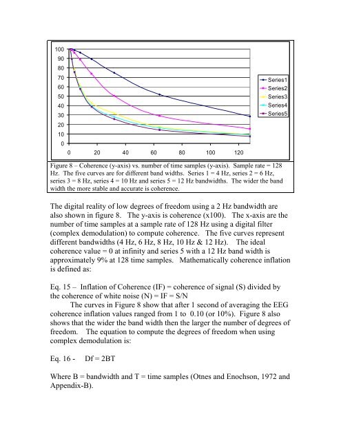
100 90 80 70 60 50 40 30 20 10 0 0 20 40 60 80 100 120 Series1 Series2 Series3 Series4 Series5 Figure 8 – Coherence (y-axis) vs. number of time samples (y-axis). Sample rate = 128 Hz. The five curves are for different band widths. Series 1 = 4 Hz, series 2 = 6 Hz, series 3 = 8 Hz, series 4 = 10 Hz and series 5 = 12 Hz bandwidths. The wider the band width the more stable and accurate is coherence. The digital reality of low degrees of freedom using a 2 Hz bandwidth are also shown in figure 8. The y-axis is coherence (x100). The x-axis are the number of time samples at a sample rate of 128 Hz using a digital filter (complex demodulation) to compute coherence. The five curves represent different bandwidths (4 Hz, 6 Hz, 8 Hz, 10 Hz & 12 Hz). The ideal coherence value = 0 at infinity and series 5 with a 12 Hz band width is approximately 9% at 128 time samples. Mathematically coherence inflation is defined as: Eq. 15 – Inflation of Coherence (IF) = coherence of signal (S) divided by the coherence of white noise (N) = IF = S/N The curves in Figure 8 show that after 1 second of averaging the EEG coherence inflation values ranged from 1 to 0.10 (or 10%). Figure 8 also shows that the wider the band width then the larger the number of degrees of freedom. The equation to compute the degrees of freedom when using complex demodulation is: Eq. 16 - Df = 2BT Where B = bandwidth and T = time samples (Otnes and Enochson, 1972 and Appendix-B).
Page 1 and 2: (unpublished manuscript - Version 1
Page 3 and 4: 29- Definition of the Cross Channel
Page 5 and 6: possible and this is why the cospec
Page 7 and 8: is because there are relatively lon
Page 9 and 10: Fig. 1 - Illustration of volume con
Page 11 and 12: Fig. 3- Example of cospectrum (in-p
Page 13 and 14: coefficient is a valid and importan
Page 15 and 16: Eq. 1- r = ∑ N ∑ N ( X ( X −
Page 17 and 18: Fig. 5 - Comparisons between the Br
Page 19 and 20: to a Pearson product-moment correla
Page 21 and 22: constitute the basis for all spectr
Page 23 and 24: The frequency analysis of a time se
Page 25 and 26: That is, the cross-spectrum power i
Page 27: Demo). 11- Third Compute Coherence
Page 31 and 32: frame” of consciousness (Thatcher
Page 33 and 34: Fig. 9 - Various degrees and types
Page 35 and 36: Fig. 10 - Illustrations of phase re
Page 37 and 38: when the 1 st derivative of the pha
Page 39 and 40: Fig. 13 shows an example of two 10
Page 41 and 42: Figure 15 - The x-axis are differen
Page 43 and 44: Fig - 16. Top is coherence (y-axis)
Page 45 and 46: Coherence inflation is defined as a
Page 47 and 48: time over which the average is comp
Page 49 and 50: Nonetheless, “instantaneous” ph
Page 51 and 52: Example of conventional digital EEG
Page 53 and 54: score; 2- Simplification by providi
Page 55 and 56: the brain. The integration of QEEG
Page 57 and 58: Multiple frequencies and multiple m
Page 59 and 60: Example of one of the progress char
Page 61 and 62: advantage of imaging of non-cortica
Page 63 and 64: where n is the number of observatio
Page 65 and 66: Fig. 22 - Illustration of phase str
Page 67 and 68: measure of the area under the curve
Page 69 and 70: Fig. 24 - Top is filtered EEG at 25
Page 71 and 72: Fig. 26 - Top is the spontaneous EE
Page 73 and 74: 27- How to compute Auto-channel Cro
Page 75 and 76: 30- Cross-Channel Cross-Frequency C
Page 77 and 78: degrees or radians and is “normal
Page 79 and 80:
exhibits statistically significant
Page 81 and 82:
www.appliedneuroscience.com 37 - Co
Page 83 and 84:
elationships as defined by the phas
Page 85 and 86:
Fig. 33 - Example of phase differen
Page 87 and 88:
Fig. 35 - Example of 4 different fr
Page 89 and 90:
Fig. 37 - Example of a measure of c
Page 91 and 92:
Fig. 39- Illustration of how cross-
Page 93 and 94:
Fig. 41- Example of cross-frequency
Page 95 and 96:
Gray, C.M., Konig, P., Engle, A.K.
Page 97 and 98:
localization and functional connect
Page 99 and 100:
35 - 48, 2007. Thatcher, R.W., Bive
Page 101 and 102:
Cannon, R., Lubar, J., Sokhadze, E.
Page 103 and 104:
Lubar, J., Congedo, M. and Askew, J
Page 105 and 106:
Yoo, S. S. et al. Increasing cortic
Page 107 and 108:
F and likewise, F iω0t iϕ t [ y e
Page 109 and 110:
6- Phase Delay or phase difference
show all

EEG and Brain Connectivity: A Tutorial - Bio-Medical Instruments, Inc.

You also want an ePaper? Increase the reach of your titles

Delete template?

Save as template?