EEG and Brain Connectivity: A Tutorial - Bio-Medical Instruments, Inc.

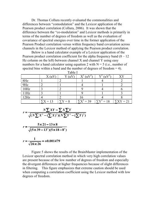
Dr. Thomas Collura recently evaluated the commonalities and
differences between “comodulation” and the Lexicor application of the
Pearson product correlation (Collura, 2006). It was shown that the
difference between the “co-modulation” and Lexicor methods is primarily in
terms of the number of degrees of freedom as well as the evaluation of
covariance of spectral energies over time in the former application of the
Pearson Product correlation versus within frequency band covariation across
channels in the Lexicor method of applying the Pearson product correlation.
Below is a hand calculator example of a Lexicor application of the
Pearson product correlation coefficient for the alpha frequency band (8 – 12
Hz column on the left) between channel X and channel Y using easy
numbers for a hand calculator using equation 2 with N = 5 (i.e., number of
spectral bins within a band and the number of degrees of freedom = 4).
Table I
X (uV) Y (uV) X 2 (uV 2 ) Y 2 (uV 2 ) XY
8Hz 1 2 1 4 2
9Hz 2 1 4 1 2
10Hz 3 2 9 4 6
11Hz 3 1 9 1 3
12Hz 4 2 16 4 8
∑X = 13 ∑Y = 8 ∑X 2 = 39 ∑Y 2 = 18 ∑XY = 21
r
r
=
=
( N
N∑ XY − ∑ X∑Y
2
2
2
∑ X − ( ∑ X ) )( N∑Y
− ( ∑
5 × 21 − 13 × 8
2
2
(5 × 39 − 13 )(5 × 18 −8
)
Y )
2
)
r
=
1
26 × 26
= + 0.001479
Figure 5 shows the results of the BrainMaster implementation of the
Lexicor spectral correlation method in which very high correlation values
are present because of the low number of degrees of freedom and especially
the divergent differences at higher frequencies because of slight differences
in filtering. This figure emphasizes that extreme caution should be used
when computing a correlation coefficient using the Lexicor method with low
degrees of freedom.