On the Ecology of Mountainous Forests in a Changing Climate: A ...

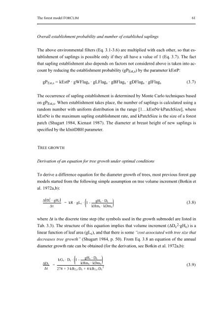
The forest model FORCLIM 61
Overall establishment probability and number of established saplings
The above environmental filters (Eq. 3.1-3.6) are multiplied with each other, so that establishment
of saplings is possible only if they all have a value of 1 (Eq. 3.7). The fact
that sapling establishment also depends on factors not considered above is taken into account
by reducing the establishment probability (gP Est,s ) by the parameter kEstP:
gP Est,s = kEstP · gWFlag s · gLFlag s · gBFlag s · gDFlag s · gIFlag s (3.7)
The occurrence of sapling establishment is determined by Monte Carlo techniques based
on gP Est,s . When establishment takes place, the number of saplings is calculated using a
random number with uniform distribution in the range [1…kEstNr·kPatchSize], where
kEstNr is the maximum sapling establishment rate, and kPatchSize is the size of a forest
patch (Shugart 1984, Kienast 1987). The diameter at breast height of new saplings is
specified by the kInitDBH parameter.
TREE GROWTH
Derivation of an equation for tree growth under optimal conditions
To derive a difference equation for the diameter growth of trees, most previous forest gap
models started from the following simple assumption on tree volume increment (Botkin et
al. 1972a,b):
∆ D c2 · gH c
∆t
= kR ⋅ gL c ⋅ 1 -
gH c · D c
kHm s · kDm s
(3.8)
where ∆t is the discrete time step (the symbols used in the growth submodel are listed in
Tab. 3.3). The structure of this equation implies that volume increment (∆D c2·gH c ) is a
linear function of leaf area (gL c ), and that there is some “cost associated with tree size that
decreases tree growth” (Shugart 1984, p. 50). From Eq. 3.8 an equation of the annual
diameter growth rate can be obtained (for the derivation, see Botkin et al. 1972a,b):
∆D c
∆t
kG s ⋅ D c ⋅ 1 -
gH c · D c
=
kHm s · kDm s
2
274 + 3⋅kB 2,s ⋅D c + 4⋅kB 3,s ⋅D c
(3.9)