Report - Terrestrial Systems Ecology - ETH Zürich

SYSTEMöKOLOGIE ETHZ
SYSTEMS ECOLOGY ETHZ
Bericht / Report Nr. 8
ModelWorks
An Interactive Simulation Environment for
Personal Computers and Workstations
Andreas Fischlin
&
Olivier Roth, Dimitrios Gyalistras, Markus Ulrich, and Thomas Nemecek
ModelWorks 2.0
Zürich, Juni / June 1990
Eidgenössische Technische Hochschule Zürich ETHZ
Swiss Federal Institute of Technology Zurich
Departement für Umweltnaturwissenschaften / Department of Environmental Sciences
Institut für Terrestrische Ökologie / Institute of Terrestrial Ecology

The System Ecology Reports consist of preprints and technical reports. Preprints are articles,
which have been submitted to scientific journals and are hereby made available to
interested readers before actual publication. The technical reports allow for an exhaustive
documentation of important research and development results.
Die Berichte der Systemökologie sind entweder Vorabdrucke oder technische Berichte.
Die Vorabdrucke sind Artikel, welche bei einer wissenschaftlichen Zeitschrift zur Publikation
eingereicht worden sind; zu einem möglichst frühen Zeitpunkt sollen damit diese
Arbeiten interessierten LeserInnen besser zugänglich gemacht werden. Die technischen
Berichte dokumentieren erschöpfend Forschungs- und Entwicklungsresultate von allgemeinem
Interesse.
Adresse der Autoren / Address of the authors:
Dr. A. Fischlin, Dr. O. Roth, D. Gyalistras, T. Nemecek
Systemökologie ETH Zürich
Institut für Terrestrische Ökologie
Grabenstrasse 3
CH-8952 Schlieren/Zürich
S W IT Z E R L A N D
e-mail: sysecol@ito.umnw.ethz.ch
Dr. M. Ulrich
Institut für Gewässerschutz und Wassertechnologie
ETH Zürich
EAWAG
CH-8600 Dübendorf
S W IT Z E R L A N D
© first print1990 Systemökologie ETH Zürich
reprinted 2011

ModelWorks
An Interactive
Simulation Environment
for Personal Computers
and Workstations
by
Andreas Fischlin ‡
&
Olivier Roth ‡ , Dimitrios Gyalistras ‡ ,
Markus Ulrich § , and Thomas Nemecek ‡
ModelWorks Version 2.0
Zürich, May 1990
Abstract
ModelWorks is a modeling and simulation environment in
Modula-2 specifically designed to be run interactively on
modern personal computers and workstations. It supports
modular modeling by featuring a coupling mechanism between
submodels and unrestricted number of state variables, model
parameters etc. up to the limits of the computer resources. It
allows for the formulation of continuous time, discrete time as
well as continuous and discrete time mixed models. Finally
ModelWorks offers in its interactive simulation environment a
handy user interface featuring efficient alterations of model and
simulation run parameters.
‡
Systems Ecology Group, Institute of Terrestrial Ecology, Department of Environmental Sciences, Swiss Federal Institute of Technology,
ETH-Zentrum, CH-8092 Zürich, Switzerland
§ EAWAG - Swiss Federal Institute of Water Resources, Water Pollution and Water Control, CH-8600 Dübendorf, Switzerland

ModelWorks 2.0
Contents
ABOUT MODELWORKS AND THIS TEXT.......................................................................5
ACKNOWLEDGEMENTS .................................................................................................7
Part I - Tutorial
1 GENERAL DESCRIPTION.........................................................................................10
2 GETTING STARTED WITH THE SIMULATION ENVIRONMENT ................................16
2.1 The Sample Model ............................................................................................16
2.2 Simulating the Sample Model ...........................................................................17
2.2.1 Default simulation .....................................................................................18
2.2.2 Changing initial values ..............................................................................19
2.2.3 Changing parameters .................................................................................19
2.2.4 Changing scaling .......................................................................................20
2.2.5 Changing monitoring .................................................................................20
2.2.6 Changing parameters during simulation ....................................................22
2.2.7 Changing integration methods ...................................................................23
2.2.8 Program termination ..................................................................................24
3 GETTING STARTED WITH MODELING ....................................................................25
3.1 The Model Definition Program of the Sample Model ......................................25
3.2 Developing a New Model..................................................................................28
3.2.1 The new model ..........................................................................................28
3.2.2 Model definition program for the new model............................................29
3.2.3 Compilation of the new model ..................................................................31
3.2.3 Simulation of the new model .....................................................................32
Part II - Theory
4 MODEL FORMALISMS ............................................................................................36
4.1 Elementary Models............................................................................................36
4.2 Structured Models (Coupling of Submodels)....................................................38
5 MODELWORKS FUNCTIONS...................................................................................46
5.1 Simulation Environment....................................................................................47
5.1.1 Program states of the simulation environment ..........................................47
1

ModelWorks 2.0
5.1.2 Simulations.................................................................................................49
5.1.2.a Simulation session ............................................................................51
5.1.2.b Structured simulation (Experiment) .................................................51
5.1.2.c Elementary simulation run................................................................53
5.1.2.d Integration or time step .....................................................................53
5.1.3 Monitoring .................................................................................................55
5.1.4 IO-windows (Input-Output-windows) .......................................................58
5.1.5 Predefinitions, defaults, current values, and resetting ...............................60
5.2 Modeling............................................................................................................63
5.2.1 The model development cycle ...................................................................63
5.2.2 Structure of model definition programs .....................................................64
5.2.3 Model installation ......................................................................................64
5.2.4 Module structure of ModelWorks..............................................................65
5.2.5 ModelWorks objects and the run time system ...........................................66
5.2.6 Program states of the client interface .........................................................68
5.2.7 Programming structured simulations (Experiments) .................................68
Part III - Reference
6 USER INTERFACE......................................................................................................72
6.1 Menus and Menu Commands ............................................................................72
6.1.1 Overview over ModelWorks standard menus............................................73
6.1.2 Menu File ...................................................................................................73
6.1.3 Menu Edit...................................................................................................75
6.1.4 Menu Settings.............................................................................................76
6.1.5 Menu Windows...........................................................................................82
6.1.6 Menu Simulation ........................................................................................84
6.1.7 Optional menu Table Functions.................................................................85
6.2 IO-Windows (Input-Output-Windows) .............................................................88
6.2.1 IO-window Models ....................................................................................88
6.2.2 IO-window State variables ........................................................................90
6.2.3 IO-window Model Parameters ..................................................................91
6.2.4 IO-window Monitorable variables ............................................................93
7 CLIENT INTERFACE ..................................................................................................98
7.1 Declaring Models and Model Objects ................................................................99
7.1.1 Running a simulation session.......................................................................99
7.1.2 Declaration of models ................................................................................100
7.1.3 Declaration of state variables .....................................................................102
7.1.4 Declaration of model parameters ...............................................................103
7.1.5 Declaration of monitorable variables .........................................................104
7.1.6 Declaration of table functions ....................................................................105
7.2 Accessing Defaults and Current Values............................................................106
7.2.1 Global simulation parameters and project description...............................107
7.2.1.a Retrieval of read only current values...............................................108
7.2.1.b Modification of defaults ..................................................................108
7.2.1.c Modification of current values ........................................................109
7.2.2 Installed models and model objects ...........................................................110
7.2.2.a Modification of defaults ..................................................................110
7.2.2.b Modification of current values ........................................................111
2

ModelWorks 2.0
7.2.2.c Inter- and extrapolation with table functions ..................................112
7.3 Removing Models and Model Objects .............................................................113
7.4 Simulation Control and Structured Simulation Runs .......................................113
7.5 Display and Monitoring ....................................................................................115
7.5.1 Window operations ....................................................................................115
7.5.2 General monitoring ....................................................................................117
7.5.3 Stash filing .................................................................................................118
7.5.4 Graphical monitoring.................................................................................118
7.5.5 Simulation environment modes .................................................................120
LITERATURE..............................................................................................................123
Appendix
A ModelWorks Version and Implementations ......................................................125
B Hard- and Software Requirements.....................................................................126
B.1 Macintosh Versions......................................................................................126
B.2 IBM PC Version...........................................................................................126
C How to Work With ModelWorks on Macintosh Computers.............................127
C.1 Installation of ModelWorks .........................................................................127
C.2 How to Work With MacMETH ...................................................................129
C.3 Configuring ModelWorks ............................................................................132
C.4 How to Make a Stand-alone Application .....................................................134
D How to Work With ModelWorks on IBM PCs .................................................136
D.1 Installation ...................................................................................................136
D.1.1 Preparing installation ........................................................................136
D.1.2 Installation of GEM Desktop ............................................................137
D.1.3 Installation of the Dialog Machine ...................................................137
D.1.4 Installation of ModelWorks ..............................................................138
D.2 How to Develop Models ..............................................................................138
E How to Work With the Dialog Machine ...........................................................139
F Bug Report Form ...............................................................................................139
G Definition Modules ............................................................................................141
G.1 Optional Client Interface .............................................................................141
G.1.1 TabFunc ............................................................................................141
G.1.2 SimIntegrate ......................................................................................141
G.1.3 SimGraphUtils...................................................................................142
G.2 Auxiliary Library .........................................................................................145
G.2.1 ReadData...........................................................................................145
G.2.2 JulianDays.........................................................................................147
G.2.3 DateAndTime.....................................................................................148
G.2.4 WriteDatTim......................................................................................149
G.2.5 RandGen............................................................................................149
G.2.6 RandNormal ......................................................................................151
3

ModelWorks 2.0
H Sample Models...................................................................................................152
H.1 The Sample Model - Logistic Grass Growth Logistic.MOD .......................152
H.2 The New Model - GrassAphids.MOD .........................................................153
H.3 Sample Model Using Table Functions UseTabFunc.MOD .........................154
H.4 A Mixed Continuous and Discrete Time Sample Model
Combined.MOD .......................................................................................155
H.5 Research Sample Models .............................................................................157
H.5.1 Third order finite Markov chain Markov.MOD ................................157
H.5.2 Population dynamics of larch bud moth LBM ...................................164
I Quick References ...............................................................................................173
I.1 Dialog Machine .............................................................................................173
I.2 ModelWorks Client Interface and Optional Modules ...................................179
INDEX ........................................................................................................................183
4

ModelWorks 2.0
About ModelWorks and this Text
ModelWorks is a simulation environment to solve dynamic systems as they are used in
biology, physics, chemistry, environmental and engineering sciences to model various
processes. It is also particularly well suited to be used by university students during a
modeling course. ModelWorks can be used for simple didactic models as well as for
very complex research models.
ModelWorks allows to work with an arbitrary number of dynamic models described by
differential or difference equation systems. A global model can be separated into,
possibly hierarchically organized, submodels which exist as independent units
communicating via output-input coupling. Modular and hierarchical modeling is
supported, which is particularly useful if for instance one wishes to keep experimental
results clearly separated from a theoretical, mathematical model by formulating them as
a parallel model, or to enhance model clarity, or to build model libraries. Discrete and
continuous models can be combined in one global model, with correct data exchange
controlled by the simulation environment.
Simple mathematical models can be built with only minor programming knowledge,
whereas programming experts have full access to a powerful programming language
and may expand into any realm of sophisticated calculations still profiting from the simulation
environment and numerical algorithms provided by ModelWorks. Hence in
contrast to most existing simulation software ModelWorks fully supports the researcher
during a model development process, which often starts with a first, crude model and
ends with the most sophisticated, in every detail refined research model 1 .
ModelWorks is based on a high-level programming language which has been selected
considering the following criteria: It has been formally defined; it is general and
powerful enough to support not only numerical computations, but also a window based,
graphical user interface; on the other hand it is also simple enough to be comprehended
and mastered by the non-computer scientist having learned programming in a basic
computer science course, such as for instance taught in Pascal programming courses; on
the other hand it also offers support for the development of large and complex models
for the expert; finally and not the least, the language is available in efficient
implementations on many machines as e.g. Apple ® Macintosh ®2 , IBM ® personal
computers 3 , or Sun ® workstations 4 . Therefore we have chosen Modula-2 as the
programming language to be used for ModelWorks, currently meeting all the listed
requirements closest (WIRTH, 1988) 5 . Due to this approach ModelWorks could be
designed as a fully open system, which can be expanded or customized by the user to
any purpose he desires.
1 ModelWorks does not force the modeler to discard the simulation software together with all other
investments in learning , implementation, and testing time, or any compatibility issues, when he reaches
the limits of the simulation language; on the contrary, ModelWorks avoids the risk of having to restart
with the model implementation all over again in a high-level programming language, since it does so
from the very beginning. In contrast to a simulation language a well designed, general purpose, highlevel
programming language guarantees that anything which can be computed on a computer can be
realized. It appears that one of the reasons why so many experienced researchers almost never use
simulation software but use instead general-purpose high-level programming languages is that they avoid
the risk to have to switch techniques in the middle of a project.
2 Macintosh is a registered trademark of Apple ® Computer, Inc.
3 IBM is a registered trademark of International Business Machines Corporation.
4 Sun is a registered trademark of Sun Microsystems, Inc.
5 See the appendix for cited literature
5

ModelWorks 2.0
ModelWorks consists of a set of library modules written in Modula-2, which contain
the program parts common to any simulation, such as numerical integration algorithms,
and the tabular plus graphical display of the simulation results, or the interactive changing
of model or other simulation parameters. The variable portion, the model of interest,
is to be supplied by the user in the form of a standard Modula-2 program. It describes
the model's behavior and installs the model in the simulation environment by means
of the elements provided by the so-called client interface of ModelWorks. Modeling
and simulating with ModelWorks includes therefore three steps: a) Writing a Modula-2
program (the model definition), b) compilation, and c) execution of the program (running
simulation experiments with the model within the simulation environment).
Interactive modeling and interactive simulations are supported in ModelWorks in
several ways. The user interface of ModelWorks in the simulation environment allows
to change interactively all settings, including any simulation parameters such as the
integration method or the step length, model parameters and/or initial values of the state
variables, plus selection of the display of simulation results. Simulation results are
made visible to the user by the so-called system behavior monitoring concept: Values
of any variable may be written onto a file for future reference, written into a table, or
displayed as curves in line-charts. All data can be reset to a given default value.
Further, the model's data structure are all stored dynamically. This allows the user to
install an unlimited number of models of an arbitrary size, with an arbitrary number of
variables each, up to the limits of the hardware.
ModelWorks simulation environment is based on the Dialog Machine 1 , guaranteeing a
consistent user interface and has originally been implemented using MacMETH 2 , a fast
and efficient Modula-2 language system for the Apple ® Macintosh ® computer (WIRTH
et al., 1988). ModelWorks simulation environment runs on any machine on which the
Dialog Machine is available. If this is the case, an efficient and smooth port of
ModelWorks in a few days work is possible. Currently ModelWorks is available for
Macintosh computers with at least 512 KBytes of memory (RAM) plus at least two
floppy drives and IBM ® PCs which run under MS DOS and have 640 KBytes of
memory (RAM) plus a hard disk. For more details on particular implementations and
hard plus software requirements for specific versions, see the Appendix. This text
serves as a manual for the ModelWorks software. Since all versions are very similar
and differences are the exceptions, there exists only this one text. Differences between
versions are minor and briefly mentioned wherever appropriate.
This text is subdivided into three parts: Part I is a Tutorial containing a little tour to be
followed step by step. It suffices to learn all basic techniques, which are needed in order
to model and simulate simple models with ModelWorks. Part II explains the
Theory and concepts behind ModelWorks, in particular model formalisms and all functions
of ModelWorks. Any advanced modeling, such as modular modeling, requires to
study the theoretical part. Part III is a Reference manual containing a complete list and
description of all features of ModelWorks. Finally the Appendix contains detailed
instructions for the installation, model development cycle, and other technical details of
interest during the daily work with ModelWorks. Included are also listings of Model-
Works' definition modules, several listings of sample models, convenient quick
reference listings, and an index.
Reading Hint: Throughout this text italics are used to emphasize that the text is to be taken literally, in
particular also case sensitive. E.g. in the citation of an identifier, such as a module name like SimMaster
or if the user has to open a file or directory with a given name such as Logistic.OBM or \MW\SAMPLES.
For easier orientation, the pages, figures and tables in Part I Tutorial and II Theory are prefixed with the
letter T, in part III Reference with the letter R, and in the Appendix with the letter A. Within some parts
figures and tables are numbered separately, starting e.g. with Fig. R1 respectively Tab. A1.
1 See the appendix for availability and installation of the Dialog Machine
2 See the appendix for availability and installation of MacMETH
6

ModelWorks 2.0
Acknowledgements
The authors wish to express many thanks to Prof. Dr. Walter Schaufelberger 1 , not only
for his substantial support, but also for his unceasing encouragement, which made this
research and development only possible.
1 Current address: Project-Centre IDA or Institute of Automatic Control and Industrial Electronics,
Swiss Federal Institute of Technology Zürich (ETHZ), ETH-Zentrum, CH-8092 Zürich, Switzerland
7

ModelWorks 2.0
8

Part I - Tutorial
This tutorial describes the elementary usage of ModelWorks, i.e. you learn how to develop
and simulate models using ModelWorks.
The first chapter, General Description, describes the general, fundamental concepts
of ModelWorks .
The second chapter, Getting Started with the Simulation Environment, contains a
step by step explanation for running an existing model and getting familiar
with the simulation environment of ModelWorks.
The third chapter, Getting Started with Modeling, teaches how to develop new
models.
Having read this tutorial you will be able do develop and simulate your own, simple
models. However, if you are interested in more complex models and more advanced
techniques, this tutorial is not sufficient. In order to learn the more sophisticated features
of ModelWorks you should read part II ModelWorks Theory and the second chapter,
Client interface, of part III Reference. They contain a full and complete description
of all possibilities ModelWorks offers.
This tutorial is best read while having access to a computer and the described steps are
actually executed 1 . This requires that the reader is already familiar with his/her computer
and the usage of its software, in particular the choosing of menu commands, clicking
on objects (i.e. object selection), and the dragging of objects (e.g. moving the scroll box
in a scroll bar). Moreover it is assumed that the user knows how to operate a simple
programming editor (e.g. the desk accessory MockWrite), has a basic knowledge of the
programming language Pascal or Modula-2 and is familiar with the mathematics involved
with modeling and simulation of differential and difference equation systems.
No particular information is provided on these topics. Please refer to other texts if you
should have any difficulties with any of these subjects 2 . The appendix contains information
on how to proceed in order to install the ModelWorks software.
Reading Hint: For easier orientation, the pages, figures and tables of Part I Tutorial are prefixed with
the letter T.
1 Note that the following text assumes that you will work with the original ModelWorks version as
available on the Macintosh ® computer. If you have no access to a Macintosh ® computer, the
instructions are to be executed similarly, but may look a bit differently or behave slightly differently,
since the IBM ® PC version of the Dialog Machine is only a subset of the Macintosh ® version. A few
hints: On the IBM ® PC folders become directories, object files ending with the extension "OBM"
become linked GEM applications with the extension "APP", and in contrast to the Macintosh MS DOS
file names are truncated to 8 characters (extension excluded); note that the latter may also affect module
names. For more details see the appendix. Wherever necessary, IBM ® PC specific information has been
added in form of footnotes. Please interpret the text accordingly and accept our apology for not being
able to offer an IBM ® PC text version; note that we are a research institution, not a commercial software
company, and hence not able to maintain more than that version we use ourselves in our daily research
work; however, you should have no difficulties in following the tutorial text, since all essential features
of ModelWorks are available on the IBM ® PC version as well.
2
We recommend: Operation of the computer: Your owner's guide, e.g. Macintosh owner's guide.
Modula-2: WIRTH, N. 1988. Programming with Modula-2. Springer-Verlag, Heidelberg, New York,
4th corrected ed. Modelling: LUENBERGER, D.G., 1979. Introduction to dynamic systems - Theory,
models, and applications. Wiley, New York, 446pp.
T 9

ModelWorks 2.0 - Tutorial
1 General Description
ModelWorks is an interactive modeling and simulation environment to study the
behavior of dynamic models, which are described by differential or difference
equations. Any system described by a set of coupled, ordinary differential or difference
equations can be modeled using ModelWorks. Since ModelWorks features modular
modeling, it is also possible to mix models of different types and even simultaneously
integrate them with different integration methods.
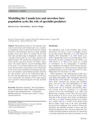
ModelWorks has two interfaces to communicate with the human user: the user
interface of the simulation environment for the simulationist and the client interface for
the modeler who builds models (Fig. T1).
Modeler
develops mod
Client Interface
ModelWorks
Simulationist
uses existing mo
User Interface
Fig. T1: The two interfaces of ModelWorks: The modeler uses the client
interface for the model development, the simulationist uses the user
interface of ModelWorks' simulation environment to perform simulation
experiments with an already existing model. Typically the modeler and the
simulationist are one and the same person changing just roles.
Typically the modeler and the simulationist are one and the same person. However
their roles are distinct and should be clearly separated: The modeler defines all
properties of a simulation model, i.e. he specifies a model definition. This includes the
specification of the model's mathematical properties and its objects, such as equations,
state variables, and parameters, plus the objects' default values and ranges. It is also the
modeler who implements the model by writing a ModelWorks model definition
program.
The simulationist runs interactive simulation experiments, hereby using one or several
models, which have been constructed by the modeler. He is restricted to use these
models within certain limitations which have been specified by the modeler, but within
that range, he may interactively define and execute with the model any kind of
experiment he wishes. For instance he may observe its temporal behavior, sample
points from particular trajectories, modify parameter values within a defined range, or
run a sensitivity analysis. ModelWorks contains all elements and algorithms needed for
computer simulations, such as numerical integration algorithms, the interactive
changing of parameter values, and the display of simulation results. The only exception
of course is the model itself, which has to be provided by the modeler.
T 10

ModelWorks 2.0 - Tutorial
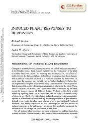
Normally a ModelWorks model definition consists of several objects, which belong to
various classes. First there must be present at least one model; but the model definition
may consist of any number of models. Second, normally each model is associated with
several objects like model equations, state variables, model parameters, auxiliary
variables, and monitorable variables. Such objects are called model objects (Fig. T2).
Model
Max initial value
State variable x(t)
x(t) = dx(t)
dt
or x(k+1)
Model parameter c
Initial value i
Min initial value
Max value
Value p
Min value
Max value of interest
Monitorable variable mv
Clipping range
Min value of interest
Fig. T2: Model objects ( ) of a ModelWorks model: A ModelWorks
model definition must consist of at least one model and every model
usually contains state variables, model parameters, and monitorable
variables. Any initial value, parameter value, minimum, or maximum value
becomes mandatory, if the associated variable or parameter is declared
within the model definition. ModelWorks maintains the actual values of
state variables, parameters, and monitorable variables and even remembers
their initially specified values (default values): ! : ModelWorks automatically
assigns the initial value i to the state variable x at the begin of
every simulation run, and the value p is assigned to the model parameter c
at the beginning of the simulation session or after any interactive change.
"# : ModelWorks uses the derivative or new value in order to compute and
repeatedly assign newly obtained values to the state variable during the
course of a simulation run (numerical integration). $ : During simulation
experiments the unknown values, which the monitorable variable mv may
obtain, shall be drawn in graphs only if they fit within a particular range of
interest; otherwise ModelWorks will clip them from the display.
A model is always of a particular type, i.e. either continuous time or discrete time. This
type is given by the kind of equations which belong to the model: In the case of
continuous time the model equations are ordinary differential equations, in the case of
discrete time they are ordinary difference equations. Note however, that a ModelWorks
model definition program may be structured, i.e. it consist of several models which may
be of a differing type, i.e. some models may be continuous time other discrete time. In
the latter case results a so-called mixed continuous and discrete time model definition.
T 11

ModelWorks 2.0 - Tutorial
A model may consist of any number of model equations. However, they must be given
as explicit, either first order differential equations or first order difference equations.
E.g. the following differential equation describing the van der Pol oscillator
y + µ(y 2 - 1)y + y = 0
is not in the proper form, since it is neither explicit nor is it first order. On the other
hand, the same equation reformulated 1 as a system of explicit, coupled first order
differential equations
x 1 = x 2
x 2 = µ(1-x 1 2 )x 2 - x 1
is now suitable to be used directly as a set of ModelWorks model equations. The
second form is called the state variable form. Most differential or difference equations
can be formulated in this form.
Usually each model uses a number of state variables. Each state variable must be
associated with a second variable used as its first order derivative in the case of
continuous time, or its new value in the case of a discrete time model. The model
equations are formulated as expressions capable of defining the values of the derivative
or new value. The expression may be an arbitrary function of any of the other model
objects, such as state variables, auxiliary variables, or model parameters. Every state
variable must be associated with a particular initial value and a range within which it
may be changed interactively (Fig. T2).
Every model may have any number of model parameters, each associated with a
particular value and a range within which it may be changed interactively. Typically
model parameters are not or only rarely changed in the middle of simulation
experiments (Fig. T2).
Intermediate results from an expression may be stored in a variable which will be later
used in another expression. Such auxiliary variables are often used to compute complex
expressions defining the value of a derivative of a state variable. In a ModelWorks
model definition program the modeler may use any number of auxiliary variables.
However in the current version, ModelWorks does neither especially recognize such
variables nor does it hinder the modeler to use them in whichever way he wishes.
Finally models may have any number of monitorable variables. They are used to
monitor the current values of any variable or otherwise accessible real numbers used in
the ModelWorks model definition program. Each monitorable variable is associated
with a clipping range used for the graphical display of the simulation results (Fig. T2).
All values specified by the modeler are remembered by ModelWorks as the so-called
default values. The values currently in use by the simulation environment are called the
current values. While starting the model definition program, ModelWorks assigns the
default values to the current values. This is called a reset. Any time the simulationist
wishes to do so, he may execute a further reset of a specific class of values, so that their
current values are overwritten with their defaults. This mechanism is most useful if the
simulationist wants to resume a well defined state before continuing with his work,
especially after having made many and complex interactive changes.
1 From the definitions x 1
= y and x 2
= y· follows x 2
· = y··, i.e. the variable substitutions y··$x· 2 , y· $x 2
,
y$x 1
; rearrange resulting two equations to make the derivatives explicit.
T 12

ModelWorks 2.0 - Tutorial
ModelWorks
Client's interface
Import list
Model definition
program
ModelWorks simulation program
Client's interface
Import list
Model definition
program
data exchange
Cotrolled data exchange
during program execution
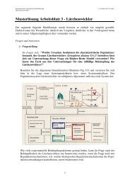
Fig. T3: Organization of ModelWorks: ModelWorks is the constant part
common to any simulation program forming the simulation environment.
The variable part, the model definition program, describes the actual model
to be simulated. Both units form together the final simulation program.
They are linked by procedures provided in the client interface and by
mutual data exchange.
Ranges for initial values of state variables or model parameters are defined solely by
the modeler. They become effective only in the simulation environment while the
simulationist edits the current values of these model objects. ModelWorks guarantees
that the simulationist assigns only values to an initial value of a state variable or a
model parameter which lie within these ranges. Hence the modeler can use this
mechanism to enforce limits within which the model equations are still valid in order to
reduce the danger that the simulationist runs a meaningless simulation experiment or
encounters a fatal error condition. However, the clipping ranges for monitorable
T 13

ModelWorks 2.0 - Tutorial
variables behave differently and should not be confounded with range limits: The
simulationist can change clipping ranges interactively anytime.
ModelWorks has been designed to make modeling as easy as possible, yet as powerful
and flexible as possible. Hence, for ModelWorks a model is a variable, not predefined
portion of a simulation program, which has been left out so that the modeler may define
it at a later time (Fig. T3). A user of ModelWorks wishes to define freely this open
portion according to his current needs, for instance by specifying a new set of coupled
differential equations. The modeler does it by writing simple Modula-2 statements,
which are to be filled in and linked to the remaining, constant parts of ModelWorks.
This is similar to a key which fits into a matching hole of a lock, only the two together
rendering the lock into a fully functional unit.
With the model definition program the modeler provides the missing key. The key
must conform to certain rules in order to fit into the hole. However, in all other aspects
this analogy breaks down, since a key is not constructed before each use anew, or must
not be extended, or has not his own particular functionality; the latter are all typical
properties of ModelWorks model definition programs.
The remaining parts of the simulation environment, i.e. the actual ModelWorks, can not
be modified and constitute the preprogrammed ModelWorks software. They are
general and hence common to any simulation program and resemble the lock with a
hole for the key. When the simulationist starts a model definition program containing a
model definition, the latter is inserted automatically into the hole of ModelWorks and
what results is a fully functional simulation program (Fig. T3).
Technically a model definition program is a simple Modula-2 program module. Its
main purpose is to define (declare) your model and its model objects, thus preparing the
data exchange needed for simulation sessions. ModelWorks does not care how the
modeler organizes the structure of the model definition program and actually knows
almost nothing about anything the modeler does in his program. The only objects
ModelWorks cares about are: models, state variables to be integrated numerically,
model parameters to be changed interactively during a simulation session, and monitorable
variables for the monitoring of the simulation results. Hence, they are the only
objects which have to be made known, i.e. declared, to ModelWorks.
The link of models and their model objects to ModelWorks is achieved via the client
interface. In its essence it consists of two library modules: SimBase and SimMaster.
These modules provide all Modula-2 objects (types and procedures) needed to describe
a model in the model definition program.
Executing a ModelWorks model definition program means to start first the simulation
environment. Running the simulation environment is called a simulation session. At
the begin of a simulation session ModelWorks initializes the simulation environment
and normally executes all model and model object declarations as programmed by the
modeler. It then performs a reset of all current values using all the defaults specified
during the declarations. Subsequently ModelWorks is ready to execute commands entered
by the simulationist, such as a simulation run, the execution of a simulation experiment,
or the editing of the current values, e.g. of a model parameter or an initial value.
ModelWorks is not just another simulation language, since a model definition program
is written as a plain Modula-2 program text. As a consequence ModelWorks can not
automatically sort the statements which compute derivatives. Compared with other simulation
software, e.g. ACSL® 1 , this may be considered to be a draw-back. However,
experience shows that automatic sorting of statements is error prone, if one models
1 ACSL® is a proprietary simulation software program that is leased with restricted rights according to
license agreement and terms and conditions by Mitchell and Gauthier Associates, Inc. (USA), Concord,
MA, respectively by Rapid Data Ltd. (Europe), Worthing, Sussex, UK.
T 14

ModelWorks 2.0 - Tutorial
complex and ill-defined systems. Moreover, the greater flexibility offered by the host
language Modula-2, a modern, powerful, and formally defined programming language,
often outweighs the lack of automatic sorting, which is mostly not much more than a
little inconvenience if the model definition has been carefully worked out before its implementation.
Most models maintain tight relationships among their objects such as state variables,
parameters, and auxiliary variables etc. The modeler may keep logically connected
objects close together, by defining related objects local to the model boundary. The
latter normally coincides with the boundary of the scope of a Modula-2 module.
Moreover, the modeler is free to use any Modula-2 feature he wishes: For instance
model objects may be part of a complex data structure or the model definition may be
spread over any number of modules, thus supporting modular modeling. This
extensibility is one of the strongest features of ModelWorks.
Even if one is not familiar with the programming language Modula-2 but knows Pascal,
it is feasible to use ModelWorks. On the other hand, ModelWorks is powerful and
flexible enough to allow also the advanced modeler to develop sophisticated models.
Note that with ModelWorks the modeler has not only full access to all features of
Modula-2, but also to those of the Dialog Machine 1 . The Dialog Machine is a
generally applicable software layer between an application program such as Model-
Works and the system software respectively hardware. In this situation the user
interacts via the the latter (mouse, keyboard, screen) only indirectly with the
application; the Dialog Machine intercepts all user interaction and filters it according to
a simple user interface. The Dialog Machine substantially facilitates the writing of
interactive programs. Not only does it simplify the programming of sophisticated
dialogs, but also does it ensure automatically a consistent man-machine interface.
Hence it allows the modeler to extend the standard, predefined ModelWorks simulation
environment easily, efficiently, and without forcing him or her first to become a
computer scientist; yet it supports an easy programming of windows, menus, bitmapped
graphics, plus mouse input. Moreover, the resulting program will be userfriendly:
Thanks to the Dialog Machine's dialog capabilities, the simulationist will be
able to enjoy the use of a simulation program, which automatically conforms to a robust
man-machine interface. This offers the advanced modeler to concentrate on the
modeling process, instead of being distracted by the cumbersome and complex
implementation details of user-interface problems. The easy access to the Dialog
Machine is another strength of ModelWorks.
For instance the modeler may wish to extend the simulation environment by
programming his own graphical monitoring in an additional, separate window or by
adding further, customized functions to the simulation environment, i.e. by installing
more menus offering additional menu commands. To give an example: ModelWorks
and the Dialog Machine have been successfully used to program an interactive
modeling environment, which allows to enter differential equations and model objects
at run time, without having to resort to any programming at all.
Despite the many features ModelWorks offers, typical model definition programs are
written in a simple, standard format. Hence, as long as one develops models without
any sophisticated extras, even the beginning programmer can quickly learn to use
ModelWorks successfully. Finally, as a simulationist only, there is no need to know
anything about the more advanced features of ModelWorks, since ModelWorks itself
has been implemented by means of the Dialog Machine. For instance, under-graduate
students at the ETHZ have been able to work successfully with ModelWorks model
definition programs within a learning time of only a few minutes.
1 The Dialog Machine has been designed by Andreas Fischlin, implemented by Andreas Fischlin, Klara
Vancso, and Alex Itten during the pilot project CELTIA under the auspices of Walter Schaufelberger
from the Swiss Federal Institute of Technology ETHZ, Zürich, Switzerland.
T 15

ModelWorks 2.0 - Tutorial
2 Getting Started with the Simulation Environment
When you read this chapter and follow the instructions given, you learn step by step,
how to run simulation experiments with ModelWorks. In particular you learn how to
produce behavior trajectories of a sample model and how to change a model's initial
and parameter values using the ModelWorks simulation environment.
It is assumed that you know how to operate the computer you are using, its operating
system, and typical application software, and that you have ModelWorks installed 1 and
are ready in order to actually perform the described procedures on your computer while
reading this chapter.
2.1 The Sample Model
The sample model is a simple growth model for grass. It models in a crude way the
growth of real grass by assuming logistic growth. In the first phase, the plants grow
exponentially under optimal conditions. Within a given, constant time interval
(doubling time), the density doubles. With increasing density, limiting factors, such as
nutrients, light energy, or competition by the neighboring plants, become more
important. This results in a decrease of the growth rate, expressed as a self-inhibition of
the plants. Finally, the grass density reaches a maximum, the so-called carrying
capacity determined by the plant's environment.
The following nonlinear differential equation describes the model:
dG(t)/dt = c 1 G(t) - c 2 G(t) 2 (1)
where
State variable:
grass (g dry weight per m 2 ):
G(t)
Initial amount of grass/initial value: G(0) = 1.0 g/m 2
Model parameters:
grass growth rate (day -1 ): c 1 = 0.7 day -1
Self-inhibition coefficient(m 2 g -1 day -1 ): c 2 = 0.001 m 2 g -1 day -1
Let us have a closer look at the model and its equation. The model has one state
variable, the grass density G(t), which is a function of time. Further, it has two constant
model parameters, c 1 and c 2 . The first term of the differential equation, c 1 G(t), describes
the exponential growth phase of the plants; the second, - c 2 G(t) 2 , is responsible
for the self-inhibition.
The unknown element in Eq. (1) is the function G(t). During a simulation, this function
is approximated by calculating a sequence of values G(t o ), G(t 1 ), G(t 2 )... given the initial
value G(t o ). Since G(t) is defined by a differential equation these computations
correspond to a particular solution of Eq. (1). In other words: By numerical integration
ModelWorks produces the trajectory going through the point G(t o ), i.e. solves an initial
1 An exact description on how to install ModelWorks is given in the appendix. Please follow these
instructions exactly, otherwise you may have difficulties while executing the described steps.
T 16

ModelWorks 2.0 - Tutorial
value problem. The sample model with the differential equation (1) has already been
programmed, compiled and is ready for execution 1 .
2.2 Simulating the Sample Model
To run the sample model, you have first to start the MacMETH Modula-2 development
shell 2 . Start it with a double click on its icon, as you start any other Macintosh
application. By the way, although there are other methods possible, it is generally recommended to
develop and simulate ModelWorks models only by working with the MacMETH shell in the here
described way 3 . To simulate the logistic grass model, choose the menu command Execute
under the menu File. A dialog box is displayed where you can select and open the
object file of the model Logistic.OBM contained in the folder Work or the folder
Sample Models on one of the ModelWorks diskettes 4 .
Upon opening this object file, you will start the ModelWorks simulation environment
linked together with the sample model. Technically speaking, this simulation program
is an ordinary MacMETH Modula-2 program running as a subprogram under the
MacMETH shell. Once fully started, you see the initial screen of the ModelWorks
simulation environment with its menu bar, and the four windows for models, state
variables, model parameters, and monitorable variables (Fig. T4).
The menu-bar has five ModelWorks menus, each with several commands: File lets you
print graphs, set preferences and quit the program; Edit allows you to access the
clipboard to transfer graphs of simulation results to other programs or to desk
accessories; Settings offers commands to set current values of the global simulation
parameters or the so-called project description plus the resetting of current values to
their defaults; Windows opens or activates the six windows of ModelWorks; and
Simulation is used to execute and control simulations. In the visible windows, the
model objects of the activated model, the grass growth model, are displayed.
Throughout this manual read instructions as e.g. "choose menu command File/Execute"
as "choose menu command Execute under menu File".
The windows initially displayed serve two purposes: First they are used to display
current values such as initial values or parameter values and secondly they are used to
enter values or settings. Hence they are called IO-windows (input-output windows).
Here are the common characteristics of the four IO-windows:
All IO-windows display a button field in the upper left corner, a list of objects in the
middle, and a scroll bar on the right side. Any model object can be selected by a simple
mouse click. All subsequent clicks on the buttons refer to the currently selected object.
Selection of the bold model title is interpreted as selection of all elements belonging to
1 On the Macintosh no preparations are necessary to follow this tutorial except that you should be using
a working copy of the software (Working through the tutorial will change the contents of your diskettes,
so don't use your originals!). On the IBM PC you are ready only if you have followed exactly the
installation procedures described in the Appendix, in particular those for the installation of the
ModelWorks software. You should have an executable GEM application made from the sample model
LOGISTIC.MOD which is now called LOGISTIC.APP.
2 On the IBM PC you have to start first the GEM desktop and then to start the application
LOGISTIC.APP. In case you should encounter difficulties up to this point, please refer to the GEM
documentation and/or check your installation (s. a. the Appendix). Ignore this and the next paragraph to
which this footnote belongs, they contain Macintosh specific information only.
3 Please refer to the Appendix for more details on the exact organization of the ModelWorks diskettes and
how to work with MacMETH.
4 In case you should have any difficulties up to this point executing the described steps on your
computer, please refer to the MacMETH documentation and/or check your installation (see also the
Appendix for detailed instructions how to install ModelWorks and a brief introduction how to work with
MacMETH).
T 17

ModelWorks 2.0 - Tutorial
this model. Selection of all objects of a list is possible by clicking the button . All
buttons with a down arrow are used to set a current value, whereas buttons with a
left arrow are used to reset a value to its default as defined by the modeler. The
button serves to specify which columns, i.e. current values of the model objects, are
to be shown in the list.
Fig. T4: Initial screen of the ModelWorks simulation environment
obtained immediately after starting the model definition program, i.e. the
module which contains the definition of the logistic grass growth sample
model. All four IO-windows for the models, the state variables, the model
parameters, the monitorable variables, plus the graph and the table window
are open. The latter two windows have been slightly rearranged from their default size
and position in order to give a better view onto the IO-windows.
The menu command Settings/ All above resets the program to its original state as it was
at the beginning of the simulation session. If you should loose the orientation during a
complex series of interactive changes, this command allows you always to resume a
well defined state.
If you should have changed already any settings up to this point, reset it first with the
menu command Settings/Reset All above before continuing with this guided tour.
2.2.1 D EF AULT S IMULATION
You can immediately start a simulation experiment (run), because ModelWorks ensures
that any valid model definition program contains all necessary data for the so-called
default simulation run. Choose the menu command Simulation/Start run to actually
start the simulation. The graph and the table windows are automatically opened, and a
small time display window appears in the upper right corner. Now, ModelWorks
integrates the differential equation and displays simultaneously the results in the graph
and table windows. In the graph window, you see how the grass grows at the beginning
exponentially and how it reaches finally its equilibrium density (Fig. T5).
T 18

ModelWorks 2.0 - Tutorial
Fig. T5: ModelWorks simulation environment during a simulation run of
the logistic grass growth sample model. In addition to the IO-windows the
table plus graph windows are currently open. The current time is displayed
in the upper right corner. The graph window shows the growth curve of the
grass (g/m 2 ).
2.2.2 CHANGING INITIAL VALUES
Initial values can be changed in the window for state variables: bring the state variable
window to the front (click on it or choose the command Windows/State variables), and
select the state variable Grass. Click on the button and change in the appearing
entry form the initial value to 4.0. This means, that the grass starts growing at a higher
density. Verify this in another simulation run; the maximal density remains the same.
Use other initial values to explore the model's behavior (e.g. 200; 0.1). If you want to
enter a initial value out of the allowed range [0,10'000], the program will refuse to
accept it. For instance try to enter 10001 or -1 and see what happens.
After your explorations, reset the initial value with the menu command Settings/Reset
All model's initial values, or with the button .
2.2.3 CHANGING P AR AMETER S
Model parameter values can be changed in the window for model parameters in the
same manner as described for initial values. Clear the graph with the menu command
Windows/Clear graph and perform a simulation run for reference purposes. What will
happen if you increase the growth rate c 1 of the grass? Faster growth, or higher
maximal density? Increase the growth rate from 0.7 to 1.2, and perform a simulation
run. Now, the population grows faster, and reaches a higher equilibrium value. In the
table output you can see the maximum value the grass density reached (%1200 g/m 2 ).
T 19

ModelWorks 2.0 - Tutorial
2.2.4 CHANGING S C ALING
As the grass curve exceeds the maximum value of 1000, ModelWorks clips these
values. In order to avoid this clipping and to have also a look at the clipped portions of
the curve, you should rescale the monitorable variable Grass. You may achieve this by
increasing the upper limit of interest for the grass. This can be done in the window for
monitorable variables. Bring it to the front, select Grass, and click on the button . In
the appearing entry form, you can enter the new scaling value for the upper limit of
interest, type 1200 and click into the OK button; ModelWorks writes the values
automatically into the legend in the graph window. Perform another simulation run.
This time, the curve should be fully visible and no longer be clipped.
2.2.5 CHANGING MONITOR ING
ModelWorks uses the expression monitoring for any kind of display of simulation results.
Any variable which can be monitored is called a monitorable variable. Every
monitoring definition is done in the window for monitorable variables. ModelWorks
uses one window for numerical display (tabulated), and one window for the graphical
display (line charts) of results, called the table window respectively the graph window.
Storage of numerical results is also supported on the so-called stash file for the use of
the data by other programs, e.g. a spread sheet program like Microsoft Excel or a
program for statistical analysis or just to document a simulation run. At a time
ModelWorks uses just one stash file only.
The model definition program of the sample model declares a second monitorable
variable beside the state variable Grass. This is the derivative of grass listed in the IOwindow
Monitorable variables with the name Grass derivative. However, the defaults
specified by the modeler for this variable are such that it is not displayed unless the
simulationist activates it for actual monitoring. To see what the curve of the derivative
looks like, bring the window for monitorable variables to the front, select Grass
derivative, and click on the button (Toggle function). In the column Monitoring
appears a "Y" in the row for the monitorable variable Grass derivative and the legend
of the graph is accordingly updated 1 . The values of the variable Grass derivative will
be drawn as another curve in the line chart of the window Graph during the next
simulation run. Running another simulation displays the two curves Grass respectively
Grass derivative.
You may generate also other graphs, e.g. Grass derivative versus Grass. Select the
monitorable variable Grass in the window for the monitorable variables window and
click onto the buttons and then .. In the column Monitoring disappears first the
"Y" and then appears a "X" in the row for the monitorable variable Grass. This means
that the values of the variable Grass will no longer be shown on the y-axis (ordinate)
(toggle function) but will be used as x-values on the abscissa. The values of the
variable Grass derivative should still be displayed as y-values (check the "Y" in the
column Monitoring and the legends for the curves and the abscissa in the graph
window). Run another simulation run and you should see a dome-shaped curve of
Grass derivative vs Grass.
Before you proceed, please select the command Reset: All model's graphing under
menu Settings.
1 This may depend on the currently set preferences, i.e. the immediate update of the graph takes place
only if the option «Once changed, immediately redraw graph» available under menu command
File/Preferences is currently checked; otherwise the redrawing of the graph will be deferred till the begin
of the next simulation run.
T 20

ModelWorks 2.0 - Tutorial
During the steps described in the previous two paragraphs you may have noticed that
ModelWorks uses different colors 1 and line patterns if you have activated several
monitoring variables at once. For instance the "Y" in the window Monitoring variables
is drawn in the same color as the corresponding curve, and curves are drawn using
different patterns (important on monochrome screens and laser printers) in order to
assist you in telling the curves apart. These characteristics of a monitoring variable are
called curve attributes and they consist of first the line style (LineStyle - the pattern with
which a line connecting two points is drawn), second the color of a curve (stain), and
thirdly the symbol with which points of a curve are marked. Unless explicitly specified,
ModelWorks assigns curve attributes automatically, which is therefore called the
automatic curve attribute definition strategy. For instance following this strategy
ModelWorks assigns automatically the stain coal (black) to the first and ruby (red) to
the second variable being activated for monitoring 2 . This helps the user to tell curves
optimally apart under many circumstances.
However, the automatic curve attributes definition strategy has also its disadvantages,
in particular the attributes may change all the time. For instance in one graph the Grass
is black, in the other it is red but Grass derivative becomes black etc. The actual color
will depend only on the exact chronological sequence in which a monitorable variable
has been activated for monitoring with the button . To try this out click on Grass
derivative in the Monitorable variables window and toggle it with button so that it
becomes activated (Y). Run a simulation, e.g. this time by pressing the command key
(clover-leaf key) simultaneously with key 'R'. Note that curve Grass is drawn in black
(unbroken) and Grass derivative in red (broken). Then click on Grass in the
Monitoring variable window and toggle it with the button twice. Again both
monitoring variables are activated (Y). Now rerun the simulation and note that this
time colors are reversed, i.e. Grass is drawn in red (broken) and Grass derivative in
black (unbroken). This is only because Grass has been activated for monitoring as the
second curve after Grass derivative which has remained untouched during the toggling
of Grass.
The convenient the automatic curve attributes definition strategy may be, the confusing
it may become in complicated situations where the simulationist wishes to run may
simulations and to compare the same monitoring variables. ModelWorks allows you to
gain complete or partial control over the assignment of curve attributes, i.e. you can
adopt your own curve attributes assignment strategy.. You may achieve this by
assigning explicitly to monitoring variables their particular curve attributes. For
instance change the color, of the curve Grass, to green and draw it with the symbol 'v'
which may remind you of real grass tuft. Click on Grass in the window for
monitorable variables, and click on the button (rainbow toggle function). . Choose
the attributes unbroken as line style 3 , the stain emerald (green), and type 'v' in the
symbol field; then click the "OK" push button. Finally select the command Set: Global
simulation parameters... under the menu Settings and change the monitoring interval to
0.5; then click the "OK" push button. Now run another simulation run and you should
see this time a green curve displaying the symbol 'v' at times 0, 0.5,1, 1.5,2 etc.
Note that from now on the curve Grass will always be drawn with exactly these curve
attributes, i.e. in green regardless when and with how many other curves you currently
display it. To see this behavior click on Grass in the Monitoring variable window and
toggle it with the button twice. Run a simulation and note that Grass will be drawn
1 On IBM PCs there are no colors available. Sorry, but the memory limitations of MS DOS have forced
us to sacrifice them.
2 the third becomes emerald (green), and the fourth sapphire (blue). For more details see part Reference.
3 Note that specifying a line style is crucial; if you should omit it, automatic definition of curve attributes
would still remain active regardless of the settings of stains or plotting symbols.
T 21

ModelWorks 2.0 - Tutorial
in green (unbroken,'v') and Grass derivative in black (unbroken) 1 . then click on Grass
derivative and toggle it with the button once, so that it will no longer be activated
for monitoring. Rerun the simulation and note that this time Grass is still drawn in
green (unbroken,'v').
Once again there is a disadvantage to this method if all your monitoring variables adopt
it: you will run more often than you may first think into a situation where several curves
currently in display happen to be all of the same color or line style (may be important
on a no-color only laser printer or a publication). For instance click on Grass in the
Monitoring variable window and click on the button , then select the line style
broken, press the space bar to clear the symbol and hit return. Now click on Grass and
activate it with button . Rerun the simulation and note that you can no longer
separate the two curves on a printer or a monochrome screen. Of course it is also
possible to switch back to the automatic assignment strategy: Select Grass and click
the button ; in the appearing entry form click into the top-most radio button
automatic definition of curve attributes and close it by pressing the enter key, or
alternatively, reset the curve attributes of variable Grass with the button or with the
command Reset: All model's curve attributes under menu Settings.
Finally you can learn how to monitor the values of the variable Grass derivative in
tabular form. Bring the window for monitorable variables to the front, select Grass
derivative, and click on the button (Toggle function). In the column Monitoring
appears a "T" in the row for the monitorable variable Grass derivative. This means that
the values of the variable Grass derivative will be written into a column of the table in
the window Table during the next simulation run. Bring the table window to the front,
enlarge it till you see all columns and rerun the simulation.
Before continuing reset this time the table and graph monitoring plus all curve
attributes to their defaults with the following method: Bring first the window Models to
the front, select the row containing the model title (Logistic grass growth model) and
click on the buttons , , and . Note that the effect of this method is exactly the
same as if you would have clicked on the buttons with the same pictures in the window
Monitorable variables after having selected the model title (bold face Logistic grass
growth model)in the latter window.
2.2.6 CHANGING P AR AMETER S DUR ING S IMULATION
Now, you will learn, how you can change model parameters even in the middle of a
simulation run. We let the model simulate the grass growth as before; but, when the
density has reached its maximal value, we increase the self-inhibition of the plants, the
parameter c 2 (this signifies, that the carrying capacity of the environment K = c 1 /c 2
decreases, for instance due to a sudden nutrient depletion or an unknown toxic
substance). After this change, the grass density will tend to a lower equilibrium value.
To do this, start a simulation with the same settings as before. When the population has
reached its maximal value (this happens approximately at time 15.0, watch the time
window), interrupt the simulation with the menu command Simulation/Halt run
(Pause). In the parameter window, you can now increase the value of the selfinhibition
coefficient c 2 from 0.001 to 0.002. continue the simulation with
Simulation/Resume run, and observe the reaction of the system.
1 Note that on a monochrome screen or a non-color printer such as a laser printer both curves are drawn
with the same line style, i.e. unbroken, and can only be separated by their different symbols 'v' resp. none.
T 22

ModelWorks 2.0 - Tutorial
2.2.7 CHANGING INTEGR ATION METHODS
To start with this section, reset the program to its initial state with Settings/Reset All
above.
The numerical integration of the differential equation has to be done with special
integration algorithms. ModelWorks offers several different methods for numerical
integration. Each has its particular advantages and disadvantages. The default
algorithm used in this example is Euler, which is shown in the model window. We
shall compare two integration methods and record the results on the stash file.
First, we have to define the stash file output. Bring the window for monitorable
variables to the front, select the variable Grass, and click on (Toggle function). In
the column Monitoring appears the letter "F" for stash filing (this is in addition to the
"T" and "Y", which signify that this variable is written already into the table and drawn
in the graph). Now, during a simulation run the values of the variable Grass will be
written also onto the stash file. Note, by default every new simulation will overwrite
the stash file's content.
Differences between integration methods become more obvious with large integration
step sizes (this is the step which is internally used for numerical integrations).
Therefore, we change this step to a higher value. Select the menu command
Settings/Global simulation parameters, and change in the entry form the value for the
integration step and the monitoring interval to 1.0. (The monitoring interval is the
interval at which simulation results are displayed. If this is smaller than the integration
step, the former is automatically reduced to generate the requested result display).
With these settings you can perform a simulation run. The integration method Euler is
the simplest integration algorithm; therefore it is fast, but not very precise. After the
integration, the stash file ModelWorks.DAT 1 , contained in the same folder as the
MacMETH shell resides, is ready for inspection and you can open it with any text
editor you have available, e.g. the desk accessory MockWrite 2 . It should contain the
same simulation results as the table window (look for look for DATA-BEGIN of
Run 1 ...).
For the next simulation choose another algorithm: Bring the model window to the
front, select the model, and click . Choose the more precise algorithm Runge Kutta
4: To prevent overwriting of the stash file, we change its name. Therefore, before
starting the next simulation run, choose first the menu command Settings/Select stash
file, and give the stash file a new name, e. g. ModelWorks.DAT2 3 . Only now start the
simulation by choosing the menu command Simulation/Start run.
The new run will give different results, as you can easily verify in the graph. For a
more detailed, numerical analysis, you could use the values on the two stash files.
ModelWorks would even allow to write the two time series onto the same stash file 4 .
1 On the IBM PC the name of this file is truncated to 8 characters and hence becomes MODELWOR.DAT.
The file resides in the same directory as LOGISTIC.APP.
2 On the IBM PC use e.g. the editor of the JPI TopSpeed Modula-2 development environment.
3 On the IBM PC use e.g. MODELWOR.DA2
4 This a more advanced technique, requiring multiple model declarations. For more details on this
subject, please refer to the reference manual.
T 23

ModelWorks 2.0 - Tutorial
2.2.8 P R OGR AM TER MINATION
The program can be terminated with the menu command File/Quit. After that, the
MacMETH environment becomes active again, ready to accept your next command, for
instance the execution of another model 1 . To return to the desktop of the Finder, use
the menu command File/Quit of the MacMETH shell.
1 On the IBM PC you will return to the GEM desktop.
T 24

ModelWorks 2.0 - Tutorial
3 Getting Started with Modeling
In this chapter you will get a closer look at the way ModelWorks models are defined.
First it is explained, how the Modula-2 program defining the logistic grass growth
sample model was written. Then you learn how to define a new model by modifying an
existing program text by using the MacMETH programming environment 1 . Finally, the
new model is made ready to be executed, i.e. simulated, using ModelWorks to start
another simulation session.
Again it is assumed that you know how to operate the computer and its software, and
that you have ModelWorks installed and ready in order to actually perform the
described steps on your computer while reading this chapter.
3.1 The Model Definition Program of the Sample Model
In the last chapter you worked with the grass growth model in the ModelWorks
simulation environment as a simulationist. Now, we shall have a closer look at the used
simulation program as a modeler. This program defines (declares) a logistic growth
model and is called a model definition program. Step by step, we shall now go through
this sample program contained in the file Logistic.MOD, and have a closer look at all its
elements. The complete listings of the program Logistic, and of the definition modules
SimMaster and SimBase, which form the client interface, are given in the appendix.
Many ModelWorks model definition programs have the same structure as
Logistic.MOD.
The import list contains all the items (types, constants, variables, and procedures) used
within the program module. They are exported by the modules which form the client
interface of ModelWorks:
FROM SimBase IMPORT
Model, IntegrationMethod, DeclM, DeclSV, DeclP, RTCType,
StashFiling, Tabulation, Graphing, DeclMV, SetSimTime,
NoInitialize, NoInput, NoOutput, NoTerminate, NoAbout;
FROM SimMaster IMPORT RunSimMaster;
RunSimMaster is the procedure, which will start the simulation environment of
ModelWorks. DeclM, DeclSV, DeclMV and DeclP are the procedures used to declare
the models and their objects. The types Model, IntegrationMethod, StashFiling,
Tabulation, Graphing, RTCType are needed in order to declare the model objects. All
these objects, i.e. models, state variables, model parameters, monitorable variables,
auxiliary variables and all associated variables, like derivatives, initial values and
default values, are typically declared locally to the program module boundaries:
VAR
m: Model;
grass, grassDot, c1, c2: REAL;
m is a variable of the opaque type Model. It allows to reference the whole model. The
logistic growth model has one state variable, and two parameters. ModelWorks
requires that state variables, monitorable variables, and model parameters are variables
of the elementary Modula-2 data type REAL. For every state variable of a
ModelWorks model, we also have to define an associated second variable of type
REAL. It either corresponds to the derivative (x(t) = dx/dt - continuous time) or the
1 On the IBM PC you have to use the JPI TopSpeed Modula-2 development environment. For more information
on how to operate it, consult the Appendix section installation or your JPI TopSpeed Modula-2
documentation.
T 25

ModelWorks 2.0 - Tutorial
new value (x(k+1) - discrete time) of the state variable (x(t) respectively x(k)). For the
sample model, which is continuous time, this is the variable grassDot.
The procedure Dynamic is the heart of a ModelWorks model definition program. It
contains the Modula-2 translation of the mathematical equations describing the model's
dynamics, here Eq. (1); for a proper functioning of ModelWorks, it is very important,
that this procedure computes the exact values of the derivatives or new values of all
state variables as required by the given equation(s):
PROCEDURE Dynamic;
BEGIN
grassDot:= c1*grass - c2*grass*grass;
END Dynamic;
The procedure Objects contains the declarations of all model objects. For each of the
four model objects, models, state variables, parameters, and monitorable variables,
there exists a special declaration procedure. Once such a procedure has been called,
ModelWorks knows the variable, defaults, plus ranges corresponding to the model
object, and can access it to maintain its values, or can show it in a window, or use it to
display its current value in a graph. It is mandatory to declare a model if you wish to
declare model objects (see below). The declaration of model objects, i.e. state
variables, model parameters, or monitorable variables is optional and depends only on
the current needs 1 .
The procedure DeclSV declares the state variable grass:
DeclSV(grass, grassDot, 1.0, 0.0, 10000.0,
"Grass", "G", "g dry weight/m^2");
The actual parameters are the two real variables for the state variable itself grass, and
its derivative grassDot. Next, there are three real constants: the default initial value,
and the upper and lower limit of the range of initial values.There is no such thing as
negative grass, hence the lower limit has been set to 0.0, the upper to a value beyond
which values are no longer plausible. The three strings are the name, an abbreviated
name, and the unit of the state variable. These strings, and the initial value, will be
displayed in the IO-windows for state variables. The limits for the initial value will be
used during interactive changes: attempts by the simulationist to enter initial values out
of the allowed range will be refused. With this mechanism the modeler can prevent the
simulationist from entering values which would result in illegal simulation experiments
for which the model is not defined or which could cause some other fatal run-time
errors.
The procedure DeclMV declares the variables grass and grassDot as monitorable
variables. This is necessary if we want to monitor the values of these variables on the
stash file, in the table, or in a graph. Typically state variables, auxiliary variables, and
output variables (used to couple submodels) are the model objects which are declared
as monitorable variables. Our calls of DeclMV:
DeclMV(grass, 0.0, 1000.0,
"Grass", "G", "g dry weight/m^2",
notOnFile, writeInTable, isY);
DeclMV(grassDot, 0.0, 500.0,
"Grass derivative", "dG/dt", "g dry weight/m^2/time",
notOnFile, notInTable, notInGraph);
1 For instance, you could use ModelWorks also for the plotting of a function, e.g. a time series measured
during an experiment (parallel model to compare measured with simulated behavior). In this case you
would need to declare only a monitorable but not a state variable.
T 26

ModelWorks 2.0 - Tutorial
The first parameter denotes the real variable, which will be monitored. Next, there are
two real constants: the default values for the scaling of the graphics output. The three
strings are the same as for the state variables: the name, abbreviated name and the unit
of the monitorable variables. The next three elements are default settings for file, table
and graph output (e.g. isY means, that by default the variable grass will be plotted on
the y-axis (ordinate) of the graph). These elements are imported with the enumeration
types StashFiling, Tabulation, Graphing.
DeclP is the procedure for the declaration of model parameters. Since we have two
model parameters, c 1 and c 2 , it is called twice:
DeclP(c1, 0.7, 0.0, 10.0, rtc,
"c1 (growth rate of grass)",
"c1", "day^-1");
DeclP(c2, 0.001, 0.0, 1.0, rtc,
"c2 (self inhibition coefficient of grass)",
"c2", "m^2/g dw/day");
The parameter list contains first the real variable of the parameter. Next, there are three
reals: the default value of the parameter, and the upper and lower limit of its range
within which the simulationist may enter a new parameter value. A parameter declared
as rtc (RTCType ) means that its value may be changed even in the middle of a
simulation, not only before or after a run. The three strings are again: the name, the
abbreviated name, and the unit of the parameter. Note that model parameters must not
be implemented as constants; since they can be changed interactively during a
simulation session, they must be Modula-2 variables.
The next procedure ModelDefinitions declares the model. It contains the following call
to procedure DeclM:
DeclM(m, Euler, NoInitialize, NoInput, NoOutput, Dynamic,
NoTerminate, Objects, "Logistic grass growth model",
"LogGrowth", NoAbout);
This declares the logistic grass growth model within ModelWorks. The first actual
parameter is the model variable m . Then, Euler (type IntegrationMethod) defines the
default integration method for this model. The next six parameters are all procedures;
Modula-2 supports procedure types and therefore it is possible to use procedures as
actual parameters when calling a procedure. This mechanism has to be used to install
in ModelWorks all procedures, which describe the model dynamics and perform the
model object declarations. It is then left to ModelWorks to actually call any of these
procedures. The procedures (No)Input, (No)Output, Dynamic describe the model's
dynamics, and the procedures (No)Initialize, (No)Terminate describe actions to be taken
at the begin and end of every simulation run (more details on the purpose and usage of
these procedures is given in the reference manual and in the definition of module
SimBase). Some of these procedure identifiers have the prefix No, which means that
these procedures have actually just empty bodies and are needed here only to call
DeclM properly. The next procedure, Objects, declares all model objects as explained
above. The next two elements are strings for the name and an abbreviated name of the
model. The last procedure, in our case (No)About, could be used to write information
about the model in the help window of ModelWorks (this window is activated by
clicking on the button in the model window).
The procedure SetSimTime sets the default values for the simulation start and stop time.
Finally, we come to the short body of the program module:
BEGIN
RunSimMaster(ModelDefinitions);
END Logistic.
T 27

ModelWorks 2.0 - Tutorial
The only action performed by this program is to call the procedure RunSimMaster.
This starts the ModelWorks simulation environment, and passes the program control to
ModelWorks. Its parameter, the procedure ModelDefinitions, contains the complete
definition of the sample model. Note, how the procedures are nested: First
ModelWorks will activate the simulation environment and call the procedure
ModelDefinitions. Later on it will call the procedure Objects; which will result again in
calls to the procedures DeclSV, DeclMV, and DeclP. This mechanism ensures that it is
clear which objects belong to which model. Note also that while declaring an object,
this object will also be immediately initialized with the given values. E.g. returning
from procedure DeclP(c,p,... will imply that the default value p for the model parameter
is assigned to the variable c.
3.2 Developing a New Model
Instead of just reading an existing model definition program we will develop a new
model. However, the new model will not be written completely anew, that would be
too cumbersome. Instead we will simply modify a copy of the sample model definition
program to develop the new model. This is an easy, hence generally recommended way
to develop ModelWorks model definition programs.
3.2.1 THE NEW MODEL
The new model does not only include grass, but also herbivores as the second state
variable aphids. Aphids feed on the grass and establish an ecological relationship, for
the sake of simplicity, we assume somehow similar to other predator-prey relationships.
The new model will consist of two coupled differential equations, each describing the
dynamics of the two species, according to the Lotka-Volterra predator-prey model 1 : the
grass is the prey, and the aphids are the predators.
The model is described with the following nonlinear second order differential equation
system; note that the parameter and initial values are not the same as in the former
model 2 :
dG(t)/dt = c 1 G(t) - c 2 G 2 (t) - c 3 G(t) A(t)
dC(t)/dt = c 3 c 4 G(t) A(t) - c 5 A(t)
(2)
where
State variables:
Grass (g dry weight [dw] per m 2 ):
G(t)
Initial amount of grass/initial value: G(0) = 200 g/m 2
Aphids (g dry weight [dw] per m 2 ):
A(t)
Initial number of aphids: A(0) = 20 g/m 2
Model parameters:
Grass growth rate (day -1 ): c 1 = 0.4 day -1
Self-inhibition coefficient(m 2 g -1 day -1 ): c 2 = 8* 10 -5 m 2 g -1 day -1
Grass consumption rate by aphids(m 2 g -1 day -1 ): c 3 = 1.5 * 10 -3 m 2 g 1 day -1
Aphids birth rate per grass consumption (g g -1 ): c 4 = 0.1 g g -1
Death rate of aphids (day -1 ): c 5 = 0.2 day -1
1 Early this century these models have first been formulated by LOTKA (1925) and VOLTERRA (1926).
Their purpose is to describe the population dynamics of a prey and a predator species.
2
The new parameter and initial values are not necessarily realistic, since the sole purpose of the model is
to help to learn ModelWorks.
T 28

ModelWorks 2.0 - Tutorial
Let us have a closer look at the new model and its equations: The first equation is the
same as before, except that the term - c 3 G(t) A(t) has been added. This term is
responsible for a decrease of the net grass growth, due to grass consumption by aphids.
The second equation describes the dynamics of the aphids: They can grow by feeding
on the grass, which is expressed with the term c 3 c 4 G(t) A(t). The second term, - c 5
A(t), accounts for the natural mortality of the aphids.
In the next section it will be explained how to alter step by step a copy of the logistic
grass growth, sample program to implement this new grass-aphids model; then the
program will be compiled and finally be simulated.
It is assumed that you know how to edit a program text, and that you are familiar with
the following terms and concepts: program text or source code, compilation, and the
execution of programs.
3.2.2 M ODEL DEF INITION P R OGR AM F OR THE NEW MODEL
The ModelWorks distribution diskettes contain an editor 1 , it is the shareware 2 desk
accessory MockWrite, a simple, straight-forward text editor. To program the new
model choose MockWrite in the Apple-menu 3 and open the file Logistic.MOD in the
folder Sample Models. We create a copy of this file with the same content by choosing
the menu command MockWrite/Save As 4 . Give the new file the name
GrassAphids.MOD 5 , and save it in the folder Work. This is the copy we shall use to
develop the new model, thus avoiding to destroy the program text of the logistic grass
growth sample model.
First change the module name. It is recommended to use the same name for the module
name as you have used to name the file containing the module, i.e. GrassAphids.
Throughout the following explanations the affected program text is shown together
with its context. The text portions actually having been altered or added are shown
underlined. At the beginning of the file
MODULE GrassAphids; (*My name, today's date*)
(***********************************)
(* Lotka-Volterra Grass and Aphids *)
(***********************************)
and at the end of the file:
RunSimMaster(ModelDefinitions);
END GrassAphids.
There is no need to change the import list. All objects required are already imported
f r o m t h e m o d u l e s SimMaster r e s p e c t i v e l y SimBase.
1 On the IBM PC an editor is part of the JPI TopSpeed Modula-2 development environment.
2 Please note that shareware does not mean it is free, but you owe the author a payment in case you use
the software on a regular basis.
3 On the IBM PC use the editor of the JPI TopSpeed Modula-2 development environment.
4 On the IBM PC use the command write to ... under the Editor Menu of the JPI TopSpeed Modula-2
development environment.
5 On the IBM PC name the file e.g. GRASSAPH.MOD.
T 29

ModelWorks 2.0 - Tutorial
Next declare the new state variable aphids, its derivative aphidsDot, and the three new
parameters c3, c4, and c5:
VAR
m: Model;
grass, grassDot, c1, c2: REAL;
aphids, aphidsDot, c3, c4, c5: REAL;
Change the procedure Dynamic by adding the consumption term into the first statement
plus inserting a second statement corresponding to the second differential equation:
PROCEDURE Dynamic;
BEGIN
grassDot:= c1*grass - c2*grass*grass - c3*grass*aphids;
aphidsDot:= c3*c4*grass*aphids - c5*aphids;
END Dynamic;
Now edit the procedure Objects . Since several default values will be different from the
ones of the old model, first change the parameters of the declaration procedures already
present. The behavior of the state variable grass is different. It needs another initial
value:
DeclSV(grass, grassDot, 200.0, 0.0, 10000.0,
"Grass", "G", "g dry weight/m^2");
The monitorable variable grass needs a new upper limit for its clipping range:
DeclMV(grass, 0.0, 10000.0,
"Grass", "G", "g dry weight/m^2",
notOnFile, writeInTable, isY);
The model parameters c1 and c2 need new default values:
DeclP(c1, 0.4, 0.0, 10.0, rtc,
"c1 (growth rate of grass)",
"c1", "day^-1");
DeclP(c2, 8.0E-5, 0.0, 1.0, rtc,
"c2 (self inhibition coefficient of grass)",
"c2", "m^2/g dw/day");
Secondly, insert the procedures declaring the variable aphids as a state and as a monitorable
variable, plus call the procedures declaring the new parameters:
DeclSV(aphids, aphidsDot,20.0, 0.0, 1000.0,
"Aphids", "A", "g dry weight/m^2");
DeclMV(aphids, 0.0, 1500.0,"Aphids", "A","g dry weight/m^2",
notOnFile, writeInTable, isY);
DeclP(c3, 1.5E-3, 0.0, 1.0, rtc,
"c3 (coupling parameter)", "c3", "m^2/g dw/day");
DeclP(c4, 0.1, 0.0, 10.0, rtc,
"c4 (ratio of grass net use by aphids)", "c4", "-");
DeclP(c5, 0.2, 0.0, 10.0, rtc,
"c5 (death rate of aphids)", "c5", "day^-1");
You could call these procedures in any order, mix declarations of state variables with
those of monitorable variables or parameter declarations. However, consider that the
T 30

ModelWorks 2.0 - Tutorial
sequence of declarations corresponds to the order in which they are listed in the I/Owindows
of ModelWorks simulation environment.
The model declaration procedure ModelDefinitions, remains the same; except for minor
changes in the actual parameters of the call to procedure DeclM. As the new model
requires a better integration algorithm, we change the default method from Euler to
Heun; further we change the model name strings:
DeclM(m, Heun, NoInitialize, NoInput, NoOutput, Dynamic,
NoTerminate, Objects, "Aphid-grass model (Lotka-Volterra)",
"GrassAphids", NoAbout);
Change the defaults for the simulation start and stop time as follows:
SetSimTime(0.0,100.0).
The main program needs no changes. 1
Once you have finished editing the new model, save it with the command Save in the
MockWrite menu, and close the MockWrite window 2 .
3.2.3 COMP ILATION OF THE NEW MODEL
Use the MacMETH shell for the compilation and execution of ModelWorks models 3 .
If you are not already in the MacMETH shell, start it now the same way as you have
done before, when you have started the simulation environment. Select the command
F i l e / C o m p i l e and type the name of your just written source program:
GrassAphids.MOD (or hit the TAB-key to choose the file with the ordinary Macintosh
file opening dialog box). Press return or click the mouse to start the compilation (or
click into the Open button).
Should you encounter any problems, e.g. the message File not found, check your
installation 4 . If the compiler finds no errors in your program, the compilation will end
with the message + :Work:GrassAphids.OBM size; else you will see the message
+ :Work:GrassAphids.RFM errors detected. In both cases, quit the compiler by
pressing the return key or clicking the mouse.
In case compiler errors have been detected, you must first correct them before you can
continue. You can ask the MacMETH shell to insert the error messages at the violating
locations in your model definition source file by following this method: Select the
menu command Merge under menu File of the MacMETH shell immediately after the
compilation. Then use the text editor to correct your errors in the model definition
program by searching for comments containing 4 hash marks ("####"); these
comments contain the compiler error messages pointing with a little arrow "†" to the
1 A complete listing of the new model is contained in the Appendix.
2 On the IBM PC use the command save file under the Editor Menu of the JPI TopSpeed Modula-2
development environment.
3 On the IBM PC use the JPI TopSpeed Modula-2 development environment. For more information on
how to edit, compile, and correct programs with it, consult the Appendix section installation or your JPI
TopSpeed Modula-2 documentation. Except for the last sentence ignore the whole section to which this
footnote belongs, it contains Macintosh specific information only. However, in contrast to the Macintosh
version you will have to add an extra step: link the compiled module and rename the resulting application
to GRASSAPH.EXE to GRASSAPH.APP.
4 Please refer to the Appendix for the installation of the ModelWorks software and the working with
MacMETH.
T 31

ModelWorks 2.0 - Tutorial
position the error has been detected 1 . E.g. if your model definition program is missing
the declaration of the parameter c 3 , then your file may look similar to this:
PROCEDURE Dynamic;
BEGIN
grassDot:= c1*grass - c2*grass*grass - c3*grass*aphids;
(* #### identifier not declared or not † visible *)
(* #### incompatible operand types † *)
aphidsDot:= c3*c4*grass*aphids - c5*aphids;
Insert your corrections and recompile your program. Execute the Merge command also
after a successful compilation in order to have the old error-messages automatically
removed (Merge always removes old error messages before it inserts any new ones). If
needed, repeat the edit-compile-merge cycle until the compiler finds no more errors.
3.2.3 S IMULATION OF THE NEW MODEL
Choose from within the MacMETH shell the menu command File/Execute 2 . A dialog
box is displayed where you can select and open the just compiled object file
GrassAphids.OBM. Note, the name of the OBM-file is defined by the name of the module, and not
by the name of the file containing the source program. To avoid confusion it is recommended to use
always the same names for files and modules.
After a while, you see the initial start-up screen of the ModelWorks simulation
environment with the new variables displayed in the I/O-windows. Execute the
following steps to explore the new model:
- Run a simulation with the default settings (Choose Simulation/Start run)
- Define a graph where the predator is plotted versus the prey (state space
curve): Select the prey, and toggle its curve definition by clicking on the
button . Click the button to define a plot which uses the x-axis (abscissa) to
plot the prey values. Start a new simulation run. The resulting curve shows
nicely how the grass and the aphids reach an equilibrium point.
- Set c 2 = 0.0 (no self-inhibition of the prey population). This results in a
different stability behavior of the system: The oscillations of the population
are no longer damped, but persist in a marginally stable limit cycle. In the
state space you may observe closed trajectories, each corresponding to such a
limit cycle. You should have obtained a graph similar to the one shown in
Fig. T6.
Marginally stable limit cycles can be easily perturbed; verify this by changing
the integration method to Euler, or while using the method Heun by increasing
the integration step and the monitoring interval up to 0.5 . How accurate is the
numerical integration algorithm?
Congratulations! You have reached the end of the introductory tour through
ModelWorks. You should have learned to develop and simulate simple models using
ModelWorks.
1 In case of difficulties with Modula-2 please refer to WIRTH, N. 1988. Programming with Modula-2.
Springer-Verlag, Heidelberg, New York, 4th corrected ed. or the MacMETH documentation (WIRTH et
al., 1988) for details on the specific MacMETH Modula-2 implementation.
2 On the IBM PC you have to start first the GEM desktop and then to start the application
GRASSAPH.APP.
T 32

ModelWorks 2.0 - Tutorial
In addition to the basic techniques you have just learned, ModelWorks features many
more advanced modeling and simulation techniques. Among the more important
features are modular, hierarchical modeling, including the coupling of several models
and the mixing of discrete time with continuous time models. With ModelWorks it is
easy to analyze results of complex simulation studies by means of a sensitivity analysis
or a parameter identification. Moreover, thanks to its architecture open for extensions
it allows for an unlimited number of possibilities. For a complete, full, and detailed
description of all of ModelWorks features, please refer to the parts Theory and Reference
of this text.
Fig. T6: Graph of the simulation results produced with ModelWorks
simulating the new, developed sample model . The graph shows a state
space representation of a Lotka-Volterra like grass-aphids model system.
In case you would like to continue with the introductory example, here some suggestions how you could
possibly explore it further on your own:
- introduce an auxiliary variable for the total biomass b(t):
b(t) = G(t) + A(t) (3)
Declare b(t) as a monitorable variable and compute its values within the procedure Output.
T 33

ModelWorks 2.0 - Tutorial
T 34

Part II: Theory
This part of the ModelWorks manual contains a description and functional specification of
every feature ModelWorks offers. However, it contains only little information on the
elementary and typical usage of ModelWorks. In case you should not be familiar with the basic
concepts of ModelWorks, please read first the ModelWorks tutorial. In particular you should
read the first chapter of the tutorial: General Description. Neither does this part of the manual
contain technical information on the actual use.
This part of the manual explains the principles behind ModelWorks, not the details on the actual
implementation and version of ModelWorks. Implementation dependent details are listed and
explained in Part III Reference of this manual. The latter has been written to support you during
your daily work with ModelWorks; this part is typically studied once, at the begin of any
serious work with ModelWorks.
This part of the ModelWorks manual contains two chapters:
The chapter Model Formalisms presents the mathematical formalisms in which
ModelWorks models are to be formulated. The first section of this chapter treats
elementary models, the second structured models, which are built from several
elementary, coupled submodels.
The chapter ModelWorks Functions describes all basic functions of ModelWorks: First
it describes the functionality of the simulation environment and secondly general
aspects of the model development process.
Any serious modeling with ModelWorks requires to read at least this part of the manual and the
section on the client interface of the manual Part III Reference.
Reading Hint: For easier orientation, the pages, figures and tables of Part II Theory are prefixed with the
letter T. Within this part the numbers of figures and tables follow those used in Part I Tutorial.
T 35

ModelWorks 2.0 - Theory
4 Model Formalisms
This chapter deals with theoretical aspects of modeling which are used in addition to the
standard knowledge when developing models with ModelWorks. Please refer to a textbook for
a general introduction to the modeling and simulation of dynamic systems 1 . In particular this
chapter explains the mathematical formalisms in which the modeler should describe
ModelWorks models. ModelWorks distinguishes between two model types: Elementary
models and structured models. Structured models are composed of several coupled, elementary
submodels.
4.1 Elementary Models
The elementary models which are used in ModelWorks are discrete or continuous time dynamic
systems. They are formally described by a set of ordinary first order differential or difference
equations. Generally model parameters are considered to be time invariant, but ModelWorks
supports time variant parameters too. However it is recommended to treat them either as
auxiliary variables (becoming part of the differential or difference equations) or to treat them as
an input. A graphical representation is given in Fig. T7. A more detailed representation is given
in Fig. T8.
( a ) ( b )
u ( t ) x ( t ) y ( t )
u (k) x (k)
y (k)
Input State Output
Input State Output
Fig. T7: Graphical representation of a dynamic system: (a) continuous time; (b)
discrete time. These systems constitute the basic types used in ModelWorks to
describe models.
A continuous time system is given by the following equations:
Dynamic equations: dx(t) = f(x(t), u(t), p f (t), t); t ! [t o ,t end ] t ! " (4.1)
Output equations: y(t) = g(x(t), p g (t), t); t ! [t o ,t end ] t ! " (4.2)
Initial conditions: x(t o ) = x o (4.3)
Input function: u(t); t ! [t o ,t end ] t ! " (4.4)
Parameter set: p(t) t ! [t o ,t end ] t ! " (4.5)
1 E.g. LUENBERGER, D.G., 1979. Introduction to dynamic systems - Theory, models, and applications.
Wiley, New York, 446pp.
T 36

ModelWorks 2.0 - Theory
A discrete time system is described by the following equations:
where:
Dynamic equations: x(k+1) = f(x(k), u(k), p f (k), k); k=k o ,..., k f-1 k ! # (5.1)
Output equations: y(k) = g(x(k), p g (k), k); k=k o ,..., k f k ! # (5.2)
Initial conditions: x(k o ) = x o (5.3)
Input sequence: u(k) = u(k o ), u(k 1 ),... u(k f ) k=k o ,..., k f k ! # (5.4)
Parameter set: p(k) = p(k o ), p(k 1 ),... p(k f ) k=k o ,..., k f k ! # (5.5)
t: Continuous time
k: Discrete time
": Set of real numbers
#: Set of integer numbers
x: State vector
dx: Derivative vector (for continuous time systems only)
u: Input vector
y: Output vector
p: Parameter vector, composed of the elements of p f and p g
(a)
p f
p g
u (t)
f
x(t)
$
x (t)
g
y(t)
(b)
p f
p g
u(k)
f
x (k+1)
T
x (k)
g
y (k)
Fig. T8: Schematic representation of a dynamic (a) continuous time or (b)
discrete time system. These systems constitute the basic types used in
ModelWorks to describe elementary and structured models.
Note that the output y defined by Eq. (4.2), resp. (5.2) does not depend on the input u. This
restriction guarantees the correct calculation of structured models. Structured models are
explained below.
T 37

ModelWorks 2.0 - Theory
In the context of ModelWorks the term output is used in a different than the usual meaning. It
is reserved to the output produced by a submodel to be connected with the input of another
submodel (coupling of submodels). It should not be confounded with the display of simulation
results for the simulationist. The latter is called monitoring.
4.2 Structured Models (Coupling of Submodels)
Any number of elementary models, in this context called submodels, may be coupled to form
complex, structured models. Any number of hierarchical levels may be introduced. Elementary
models are defined exactly the same way as described in the previous chapter. The coupling is
realized by connecting a submodel's output to another submodel's input. There are three cases
to be distinguished: (A) all submodels are continuous time systems only, (B) all submodels
are discrete time systems only, (C) and there are some continuous as well as discrete time
submodels.
u
11
u 1
x 1
y 1
y
11
u 21
1
u*
1
u 21 u x y
y*
u * 2
2 2
y *
u*
2
2
3
u
31
y 32
u 3
x 3
y 3
u 32
y 22
y*
y 31
Fig. T9: Example of a structured model system composed of three
coupled submodel systems. The global input u* is defined by Eq. (6a, elementary,
b, or c), the
inputs of the subsystems u ij by Eq. (7a, b, or c), the outputs of the subsystems y ij
by Eq. (9a, b, or c), and the global output y* by Eq. (10a, b, or c).
(A) A structured model composed of n elementary, coupled submodels, each continuous time
and defined according to Eq. (4.x) is defined as follows (for an example see also Fig. T9):
The input of the global system is given by
u* = u*(t) (global input) (6a)
The input to the submodel i depends on the global input u*, and on the output y i (t) of the n
submodels (output-input coupling):
u i (t) = h i ( u*(t) , y 1 (t),... y n (t)) (input of submodel i) (7a)
The dynamic equations for obtaining the derivatives of the state variables of the submodel i:
T 38

ModelWorks 2.0 - Theory
dx i (t)/dt = f i (x i (t), u i (t), p fi (t), t) (dynamic equations of submodel i) (8a)
The output of the submodel i depends on the states and the parameter set of the submodel i. An
output variable must not depend directly on an input variable (no direct output-input coupling).
Since the input variables may depend directly on the output variables, a direct output-input
coupling would lead to a circularity which could not be resolved generally.
y i (t) = g i (x i (t), p gi (t), t) (output of submodel i) (9a)
Some of these outputs are not connected to other submodels but are global outputs. These
elements from y i (t) form for each submodel the global output vectors y i * (t).
The output of the global system is given by combining the global output vectors y* i of the n
submodels i:
y 1 * (t)
y * (t) =
.
.
(global output)
(10a)
y n * (t)
(B) A structured model composed of n elementary, coupled submodels, each discrete time and
defined according to Eq. (5.x) is defined as follows (for an example see also Fig. T9):
u* = u*(k) (global input) (6b)
u i (k) = h i ( u*(k) , y 1 (k),... y n (k)) (input of submodel i) (7b)
x i (k+1) = f i (x i (k), u i (k), p fi (k), k) (dynamic equations of submodel i) (8b)
y i (k) = g i (x i (k), p gi (k), k) (output of submodel i) (9b)
y 1 * (k)
y * (k) =
.
.
(global output)
(10b)
y n * (k)
(C) A general structured model composed of n elementary, coupled submodels, each either
continuous or discrete time and each defined according to Eq. (4.x) resp. Eq. (5.x) is defined as
follows (for an example see also Fig. T9):
There are two different independent variables: the continuous time t ! " and the discrete time k
! #. The constant time step 1 of the discrete time submodel(s) is interpreted as a real time
interval, the coincidence interval c, on the time axis t. The discrete time submodels are only
known at the endpoints of these intervals, the coincidence time points (or coincidence points).
The continuous time submodel(s) describe continuous (or faster) processes which occur
between the coincidence points. A communication between the two submodel types occurs only
at every coincidence point (Fig. T10). By definition the coincidence interval c is a positive
integer and must have a size of at least 1. In the context of simulations it is meaningful to match
the values of the two time variables; thus at every coincidence point it must hold t = k. This
requirement is guaranteed if the following conditions are satisfied:
t o = k o and t end = k f where k o , k f ! # (11)
T 39

ModelWorks 2.0 - Theory
Any structured model mixed of continuous and discrete time submodels can be subdivided into
two portions: the first is the continuous time portion % consisting of the set of all continuous
time submodels with their related continuous time inputs and outputs plus the continuous time
global input and output; the second is the discrete time portion & consisting of the set of all
discrete time submodels with their related discrete time inputs and outputs plus the discrete time
global input and output. At every coincidence point the system is fully defined and all
submodels are fully coupled (System ~ % + &). At these points the real time t is mapped to the
discrete time k as follows:
k = INT(t) where INT yields the integral part of its argument (12)
Between coincidence points, the dynamics of the system collapse or degenerate to the
continuous time portion %, the other portion of the system & remains constant but is still
accessible to %. This corresponds to a sample and hold technique (sample at coincidence points,
hold between) (Fig. T10).
Discrete system
Continuous system
Cont. time scale: t
o
t
o
+ c
Disc.time scale: k
o
k
1
Coincidence time points
k
2
k
f
coincidence interval c
time
t
end
Fig. T10: Coupling of discrete and continuous time submodels: The figure shows
the results of a simulation of a structured model system composed of one discrete
and one continuous time submodel. A communication between the two submodels
occurs at every coincidence time point, when the output of the discrete submodel
determines the rate of change of the continuous time submodel. No data exchange
takes place during the coincidence interval, during which the rate of change of the
discrete time submodel remains constant (sample and hold).
The global input consists of two vectors, one for the global continuous time input u* ' and the
other for the global discrete time input u* ( :
u* ' = u*(t) (! %)
u* ( = u*(k) (! &)
(global inputs)
(6c)
At the coincidence points the inputs of all submodels i depend on the continuous as well as the
discrete time global input u* ' resp. u* ( , and on the output of the continuous time submodels j '
! % as well as the discrete time submodels j ( ! & (i, j ' ,j ( ! {1,2,... n}. Between coincidence
points the inputs to the continuous submodel i ' ! % depend continuously on the continuous
time global input u* ' and on the output of the continuous time submodels i ' ! %. Any
T 40

ModelWorks 2.0 - Theory
dependence of the continuous time submodels j ' ! % on the output of the discrete time
submodels j ( ! & is resolved by using the last defined values (sample) of all variables of & while
mapping time t to k using Eq. (12) (hold):
u i ' (t) = h i
' ( u* ' (t), u* ( (k) , y 1 ' (t), y 2 ' (t),... y n-1 ( (k), y n ( (k)) k = INT(t) (! %)
u i ( (k) = h i
( ( u* ' (t), u* ( (k) , y 1 ' (t), y 2 ( (k),... y n-1 ( (k), y n ' (t)) t = INT(t) = k (! &)
(7c)
The dynamic equations for the calculation of the derivatives for % or the new values for & of the
state variables of the submodels i ' resp. i ( :
dx i'
(t) = f i'
(x i'
(t), u i'
(t), p fi'
(t), t) (! %)
x i(
(k+1) = f i(
(x i(
(k), u i(
(k), p fi(
(k), k)
(! &)
(dynamics of submodels i ' , i ( )
(8c)
The output of the submodels i ' resp. i ( are calculated of the states and the parameter set of the
particular submodel i ' resp. i ( . An output variable must not depend directly on an input variable
(no direct output-input coupling, avoids unresolvable circularity).
y i'
(t) = g i'
(x i'
(t), p gi'
(t), t) (! %)
y i(
(k) = g i(
(x i(
(k), p gi(
(k), k)
(! &)
(outputs of submodels i ' , i ( )
(9c)
Some of these outputs are not connected to other submodels but are global outputs. These
elements from y i'
(t) resp. y i(
(k) form for each submodel the global output vectors y i'
)(t) resp.
y i(
)(k).
The global output y* of the structured model consists of two vectors, one for the global
continuous time output y* ' and the other for the global discrete time output y* ( . Each is again
composed from the global output vectors y i'
)(t) of the continuous time submodels i ' ! % resp.
the global output vectors y i(
)(k) of the discrete time submodels j ( ! &:
y * 1' (t)
y *' (t) =
y * 2' (t)
.
(! %)
.
.
(global outputs)
(10c)
y *( (k) =
.
*
y n-1( (k)
(! &)
y * n( (k)
The general definition of the couplinghas two special cases which are often of interest to the
modeler:
- Structured model consisting of several, but uncoupled submodels: The inputs of the
submodels do not depend on any output of another submodel: u i (t) = h i (u*(t)) resp.
u i (k) = h i (u*(k)). Such submodels coexist as completely independent units.
Implementing them in such a way offers the advantage that the models can be
simulated in parallel at once. This is useful to work simultaneously with a set of
identical or similar models, e.g. to test different model versions of the same real
system, or to compare a measured time series (parallel model) with a simulated
trajectory (model).
T 41

ModelWorks 2.0 - Theory
- The structured model is composed of hierarchically organized submodels (several
levels): An example of such a hierarchical model system is given in Fig. T11 (two
levels). Note however, that ModelWorks ignores the hierarchical organization, which
is only of concern to the modeler. ModelWorks treats all models exactly the same
way, regardless of the level on which they are declared.
u
11
u 1
y 1
u 21
1
y
11
u*
1
u 21 u x y
y*
u * 2
2 2
y *
u*
2
2
u
31
y 32
u 3
y 3
u 32
y 22
y*
y 31
Fig. T11: Example of a hierarchically organized structured model system
composed of several submodels, which are themselves structured model systems
consisting of several internally, coupled submodels.
Structuring model systems as defined in Eq. (7a,b or c) requires a particular calculation
sequence during simulation which may affect the results in a way which has to be considered by
the modeler. In particular it must ensure that all input values are calculated first, i.e. at the begin
of an integration step. Further, the results must be independent of the calculation order of the
submodels. This can be guaranteed given that the following conditions are observed:
1. The calculation of a model is split into the following three parts:
a) Calculation of the input variables u i (t) for the submodel i: Eq. (7a, b or c)
b) Calculation of the derivatives resp. the new values of the state variables of the
submodel i (integration): Eq. (8a, b, or c)
c) Calculation of the output variables y i (t) of the submodel i: Eq. (9a, b, or c)
2. The calculation order is that shown in Fig. T12.
ModelWorks guarantees that the prerequisit under point two is always met, but cannot ensure
that none of the model equations are misplaced, e.g. that a derivative is calculated in a part
reserved for the calculation of inputs.
T 42

ModelWorks 2.0 - Theory
Note also that the calculation order shown in Fig. T12 has a further consequence to be
considered by the modeler: It may affect the precision of the numerical results depending on
how the equations are distributed among the continuous-time submodels. Differential equations
coupled within a submodel are integrated differently from those coupled via submodel
boundaries when using higher order integration methods. This fact should be considered when
subdividing a model into several submodels unless the simulationist should restrict himself to
single step integration methods only (s.a. the following example and Fig. T14).
t * t' * t+h
Initial
conditions
Output of all
subsystems
Input of all
subsystems
Integration of
all subsystems
t := t + h
Fig. T12: Calculation order applied by ModelWorks during integration. The
larger loop corresponds to a single time step (h = current integration step); the inner
loop is used only by integration methods with order > 1 (e.g. Heun, Runge-Kutta
4 th order).
Fig. T12 shows how coupling within a single submodel, i.e. formulated within the equation
section dynamic, is defined at every point in time, whereas the coupling between submodels, i.e.
formulated within the equation sections output respectively input, takes place only at the end
points of an integration step. Note also that this phenomenon is different from the coupling
between continuous and discrete time submodels, where the coupling is usually happening even
more rare, i.e. only at the coincidence points. They are mostly much further apart than the
current size of the integration step h. Both kinds of coupling, the one at the end points of the
discretisation interval h as well as the one at the end points of the coincidence interval c, are of
the same type, i.e. ModelWorks applies the so-called sample and hold technique (see also below
under Simulation environment of the next chapter ModelWorks Functions).
Finally a simple example shall illustrate the whole concepts discussed in this chapter. The
model is a system consisting of two ordinary, nonlinear first-order differential equations. First
it shall be modeled simply and secondly it shall be modeled as a structured model built from
submodels:
Ex.: The following model equations shall be modeled, first within a single model (Eq. 13):
x 1 = ax 1 - bx 1
2
- cx 1 x 2
x 2 = c'x 1 x 2 - dx 2
(Model +) (13)
This system consists of two ordinary but coupled differential equations formulated according to
Eq. (8a) with neither input nor output (completely autonomous system). See Fig. T13a for the
relational diagram of this model system.
Secondly the two differential equations shall be distributed into two separated submodels (14)
respectively (15), which are coupled with each other (Fig. T13b):
u 1 = y 2
input according Eq. (7a)
x 1 = ax 1 - bx 1 2 - cx 1 u 1 dynamic according Eq. (8a) (Submodel µ1 ) (14)
y 1 = x 1
output according Eq. (9a)
T 43

ModelWorks 2.0 - Theory
respectively
u 2 = y 1
input according Eq. (7a)
x 1 = ax 1 - bx 1 2 - cx 1 u 2 dynamic according Eq. (8a) (Submodel µ2 ) (15)
y 2 = x 2
output according Eq. (9a)
Model M
x
x
1 2
(a)
Structured Model System
(b)
y
x
1
x
2
Submodel µ1 Submodel µ2
u 1
1
u
y 2
2
Fig. T13: Relational diagrams of a model once (a) formulated as a single
elementary model M given by Eq. (13) and once (b) modeled as a structured model
system consisting of two submodels µ 1 and µ 2 according to the Eq. (14) and (15).
Both submodels are of the type continuous time and case (A) applies with the equations (6.a)
till (10a), but no global inputs nor global outputs are present. Each of these submodels has one
input and one output defined according to Eq. (7a) and (9a). These inputs and outputs have
only been introduced in order to couple the two submodels. They form a structured model
system, each submodel containing one of the differential equations from Eq. (13).
Mathematically the structured model system formed with (14) and (15) is equivalent to the one
given by Eq. (13). However, discretisation errors may result in the sample and hold effect
described above (see also below under Simulation environment of the next chapter) (Fig. T14).
This is because no information exchange across submodel boundaries takes place during an
integration step. Thus coupling among submodels occurs only at the endpoints of an
integration step (s.a. Fig. T12). In case a higher order integration method is used, the coupling
of differential equations within a submodel takes place even in the middle of an integration step.
Hence simulation results of the continuous-time part of a structured model might slightly differ
for non-single step integration routines depending on where the modeler has chosen the
submodel boundaries between the differential equations. However the smaller the integration
step, the smaller becomes this effect . E.g. in order to make the effect clearly visible, case (ii) of
Fig. T14 has been computed with a rather large integration step of h=0.15.
T 44

ModelWorks 2.0 - Theory
(i)
(ii)
Fig. T14: Simulation results of two mathematically equivalent model variants a and
b as given by Eq. (13) respectively Eq. (14-15). Results obtained using (i) - the
first order Euler, (ii) - the second order integration method Heun with steplength h
= 0.15. Although the two model variants (s.a. Fig. T13) ought to behave identically,
their two implementation variants a and b yield the same results only in case (i), but
differing ones in case (ii). This is a consequence of the calculation order within a
simulation step (Fig. T12) and the order of the integration method: In case (ii) the
information exchange between submodels is not so often done for variant b than for
variant a, because it takes only place at the begin of, not during an integration step.
x 1a , x 2a - state variables of variant a; x 1b , x 2b - of variant b.
T 45

ModelWorks 2.0 - Theory
5 ModelWorks Functions
ModelWorks functions are available in two ways: First by the simulationist in the simulation
environment of ModelWorks and second by the modeler via the client interface (Tutorial
Fig. T1). The simulation environment allows to access the ModelWorks functions interactively
by the simulationist, the client interface to access them in a static predefined way, i.e. through the
writing of a model definition program (Tutorial Fig. T3) by the modeler. Both techniques have
their unique advantages and disadvantages.
The simulation environment of ModelWorks provides the run-time environment to define simulation
experiments, e.g. by changing parameter values, to execute simulation runs, and to control
the monitoring of the simulation results. A simulation run of ModelWorks corresponds to the
numerical solution of an initial value problem of a set of ordinary differential equations or
difference equations alone or in any mixed form. In particular note that this means that the current
implementation of ModelWorks does neither provide a direct support for the solution of
boundary value problems nor does it offer backward numerical integration.
All activities from the starting of the simulation environment till its quitting are termed a simulation
session. In essence it is nothing else than the execution of the procedure RunSimMaster
from module SimMaster. Values or attributes of the models plus their objects and the monitoring
can be changed interactively from within the simulation environment for the following settings
and parameter values:
- Global parameters and settings:
• start and stop time for simulation runs
• integration step 1 respectively maximum integration step plus maximum relative
local error 2 ,
• discrete time step (coincidence interval) 3
• monitoring interval
• project description consisting of a title, remark, and footer string plus parameters
which control the display of strings in the graph respectively the recording of
information on models and model objects together with their current values and
settings on the stash file (recording flags)
• stash-file name
- Model specific attributes:
• integration method
- Model objects specific attributes:
• initial values of state variables
• values of model parameters
• kind of monitoring and scaling for monitorable variables
In addition, the simulation environment of ModelWorks offers a versatile reset mechanism
which allows to reset any parameter or setting which may have been changed interactively during
the simulation session by the simulationist or via the client interface by the model definition
1 only if at least one continuous time (sub)model is present
2 only if at least one continuous time (sub)model with a variable step length integration method is present
3 only if at least one discrete time (sub)model is present
T 46

ModelWorks 2.0 - Theory
program. The values or settings to which ModelWorks resets are the so-called default values
originally specified by the modeler via the client interface. This allows the simulationist to return
any time to a well defined state of all parameters and settings. Further details on how to use
ModelWorks during a simulation session can be found below in the section on the Simulation
environment of this chapter.
The client interface is used to define, i.e. to declare the models, the model objects, the model
equations, and the default values for all objects so that the run time system of ModelWorks may
access and maintain them (Tutorial Fig. T2). It is important to note that ModelWorks does only
know about those objects which have been made known to ModelWorks, i.e. which have been
explicitly declared. Otherwise ModelWorks does not care what the modeler is doing with these
objects, nor whether they are part of a complicated structure. For instance a state variable might
be computed by retrieving values from a data base or might be part of a structured type such as a
Modula-2 record or an array. On the other hand it is also important to understand that
ModelWorks will perform calculations on objects, i.e. will assign values. E.g. at the begin of a
simulation run ModelWorks assigns automatically the initial values to all state variables or updates
the values of state variables during the simulation by assigning to them the results of numerical
integrations. In order to use ModelWorks meaningfully it is necessary that the modeler
obeys a minimum number of rules, so that ModelWorks and the modeler use and access model
objects in harmony. The client interface has been designed to warrant this harmony automatically
to a large extent as well as to offer the modeler at the same time as much flexibility as
possible.
The modeler may also program a structured simulation, a so-called ModelWorks experiment.
Typically an experiment consists of many simulation runs and will call ModelWorks functions
similar to the way the simulationist would use them. The latter is important if the simulationist
is to be relieved from cumbersome, repetitive command sequences or if simulations are used as
parts of more complicated procedures. For instance in order to create a phase portrait the simulationist
would have to assign a series of different initial values to the state variables as well as to
start after each assignment a simulation run. All this can be easily accomplished by programming
a structured simulation which the simulationist then can activate by a single command
from within the simulation environment. Other examples are: After a model has been
thoroughly explored interactively it is to be used for a sensitivity analysis or parameter identifications;
both examples requiring the writing of special program sections, a task which is well
supported by ModelWorks client interface.
Moreover ModelWorks allows to extend its functions via the client interface. Since
ModelWorks is based on the Dialog Machine the modeler may also access Dialog Machine
routines himself and mix them with the functions provided by ModelWorks alone. For instance
the modeler might want to have an additional kind of monitoring not offered by the standard
ModelWorks functions. To accomplish this he may add a new menu with commands to open a
window in which simulation results are to be displayed in a problem specific graph, e.g. by
coloring areas in a map according to the current values of model variables. Besides, since model
objects belong to the model definition program and are fully accessible, the latter poses no
problem for the modeler. Further details on the use of ModelWorks via the client interface are
given below in the section Model development of this chapter.
5.1 Simulation Environment
5.1.1 P R OGR AM S TATES OF THE S IMULATION ENVIR ONMENT
During a simulation session ModelWorks is always only in one of three states: No simulation,
Simulating, or Pause (Fig. T15). States are characterized by the availability of certain commands.
In the state No simulation model and model object attributes can be interactively
changed. In the state Simulating user interactions are limited, e.g. IO-windows are inactivated.
In the state Pause the simulation is temporarily brought to a halt to allow for interactive changes
T 47

ModelWorks 2.0 - Theory
of parameters. Limitations have been introduced to ensure consistency and because certain
commands are meaningful only in particular states.
(a) Menubar and menu commands
(b) Program states and transition commands of menu Simulation
No simulation
Menu status:
I/O-window status:
Start run or Stop (kill) run or
Execute Experiment Stop time reached or
Termination condition true
Menu status:
Simulating
I/O-window status:
Stop (kill) run
Resume run
Halt run (Pause)
Menu status:
Pause
I/O-window status:
Fig. T15: Menu commands (a) and state transition diagram (b) of the simulation
environment of ModelWorks. The simulation environment is always in one of the
following three states: No simulation, the state in which the simulationist may
change values or settings, e.g. simulation time, initial values of state variables, or
values of model parameters. During a simulation run or a structured simulation experiment
ModelWorks is in the state Simulating. In this state the simulationist may
only temporarily pause or stop (kill) the running simulation. The state Pause allows
to change model parameters with the attribute RTC (Run Time Change) set, or
to resume respectively abort the simulation. For every state the status of the menu
commands is symbolized as follows: A black line signifies an active, a grey an
inactive or unavailable menu command. The availability of the button commands of
a particular IO-window is indicated by a black (object selection possible, all buttons
active) or grey (disabled selection, inactive buttons) window title bar.
T 48

ModelWorks 2.0 - Theory
For instance changing a parameter value while a simulation is running is prohibited, i.e. may not
be issued in the state Simulating, in order to avoid the display of incorrect simulation results; or
the command to stop a simulation is meaningless if there is no simulation run in progress, i.e.
this command is available only in the states Simulating or Pause. In particular this design also
ensures that the simulationist can not start a second simulation run on top of an already running
one unless the first one has been terminated. The current states can be determined by the
modeler via the client interface by calling the procedure GetMWState.
Transitions from one state to another are accomplished in several ways: Either the simulationist
decides to issue a menu command available under the menu Simulation, or ModelWorks leaves
the state Simulating due to one of the following two reasons: The simulation time has reached
the stop time, or the terminate condition provided by the modeler returns true. Note that this
implies that state transitions are under the control of either the simulationist or of the modeler,
and/or are automatically controlled by the ModelWorks run time system. In case of conflict the
commands of the simulationist have the highest priority followed by the conditions programmed
by the modeler. It is possible to quit the simulation environment from within every
ModelWorks state (menu command Quit).
5.1.2 S IMULATIONS
After starting an existing model definition program, i.e. execution of the procedure
RunSimMaster the ModelWorks simulation environment appears on the screen with its
menubar and the four IO-windows, one for each kind of model objects (Tutorial Fig. T4). They
display the information, current settings and values of all model(s) and all model's objects. Any
model object is recognized by ModelWorks only if it has been declared during execution of the
corresponding declaration procedure. The latter is given by the actual parameter used while
calling procedure RunSimMaster. Choosing the menu command Quit results in the termination
of the procedure RunSimMaster, i.e. the simulation session is terminated and the simulation
environment is left. All models and all model objects will cease to exist. The reverse is true
also: The modeler must be careful to ensure that all models and model objects exist as long as
the simulation session lasts; otherwise ModelWorks will not function properly. In particular
this means that models or model objects variables such as state variables must never be declared
as variables local to a Modula-2 procedure.
After startup, the simulationist has the choice either to start immediately a simulation with the
predefined default values or to change interactively any settings. The client interface has been
designed such that the modeler can't make an error by unintentionally leaving out a needed value
to define fully the initial value problem of a ModelWorks simulation run. During simulations
two additional windows, the graph and the table window, are automatically opened or brought to
the front for the display of the simulation results. Simulation results may also be written to a
so-called stash file for future references by ModelWorks or other application software such as a
spreadsheet or a statistics program. Simulations and interactive changes of parameter values or
settings can be done freely in any order.
To issue a command to ModelWorks the simulationist has several options: First the omnipresent
menu bar offers a set of pull-down, pop-up, or tear-off menu commands; second some
menu commands (their menu text is followed by "…") will open so-called entry forms offering
from one to several editable fields to enter numbers or change settings via check boxes etc.
Thirdly the so-called IO-windows allow to select particular models or model objects for modifications
or to issue further commands. The use of menus, menu commands, and entry forms are
intuitively appealing, easy to understand, and follow the user interface of the Dialog Machine
described elsewhere (see Appendix and Literature).
There hold certain relationships among the tasks which are performed by ModelWorks during a
simulation session (Fig. T16). Tasks are nested and each belongs to a particular, hierarchical level:
T 49

ModelWorks 2.0 - Theory
Execution of procedure md 1
Simulation session
Reset All
Reset all
Initialize simulation session
Initialize session
Structured simulation (Experiment)
Initialize experiment
Simulation run
Initialize run
n
k
i
Output, Input
Dynamic
Terminate run
Terminate experiment
Fig. T16: Relationships among the nested ModelWorks tasks performed during a
simulation session. The simulationist may execute an arbitrary number n of structured
or elementary simulation runs. A structured simulation (experiment) consists
of an arbitrary number k of elementary runs. Every elementary simulation run
consists of the sections Initialize, dynamic (includes the sections Output, Input, plus
Dynamic s.str.), and Terminate. The dynamic section is executed according to the
chosen time step and simulation time an arbitrary number of times i. Unless defaults
were changed a simulation session can be fully reset to the original start-up
conditions (Reset all).
1 argument passed in call to procedure RunSimMaster
T 50

ModelWorks 2.0 - Theory
5.1.2.a
Simulation session
The simulation session (Fig. T16) consists of all activities done by means of the ModelWorks
simulation environment during the execution of a typical model definition program. It represents
the topmost level of all simulation tasks and corresponds to the execution of the procedure
RunSimMaster from module SimMaster. It may be repeated with the same set of models as
many times the simulationist wishes, but otherwise there are no relationships to other simulation
tasks on the same level. In particular ModelWorks does not support any communication of data
from a simulation session to another one except for the simulation results contained in the stash
file. Neither does the current version of ModelWorks support the direct reading of the stash
file. However, it is possible to construct a particular model which reads a stash file and declares
the models and model objects needed for a post run analysis. ModelWorks writes data onto the
stash file according to a syntax particularly designed for this purpose.
When ModelWorks enters a simulation session it always first executes a full reset (Fig. T16),
i.e. it ensures that all current values to be used during the session have exactly the values as defined
by the so-called defaults (s.a. chapter Predefinitions, defaults, current values, and resetting).
Defaults can stem from different sources, i.e. they are either predefined by ModelWorks
or have been specified by the modeler via the client interface.
Next ModelWorks initializes the simulation session (Fig. T16). The modeler can customize
this initialization, e.g. in order to add an additional menu or to set particular defaults etc. This
can be accomplished by installing an initialization procedure with a call to the procedure
DeclInitSimSession from SimMaster before calling procedure RunSimMaster. ModelWorks
will then automatically call the installed initialization procedure at the begin of a simulation session
or whenever the simulationist requests this via the corresponding menu command provided
in the simulation environment.
After the reset and the initialization, the program state is always NoSimulation (Fig. T15).
5.1.2.b
Structured simulation (Experiment)
This level can be accessed by the simulationist by choosing the menu command Execute experiment
under menu Simulation. It is the next level below that of the simulation session
(Fig. T16). A structured simulation works similar to an elementary simulation run but differs
slightly in the following aspects: Basically it is a procedure programmed by the modeler; typically
it calls several elementary simulation runs by calling the procedure SimRun from module
SimMaster. Since it is implemented as a client provided procedure, where the modeler has
anyway already full control, no experiment specific initialization and termination procedures for
experiments are offered by ModelWorks.
Structured simulations are optional and have to be installed first by the modeler via the client
interface before they can be executed by the simulationist. If no experiment is known to
ModelWorks this is the same as leaving this level out completely. Note also the simulationist
may always bypass this level by directly starting an elementary simulation run.
The simulationist can execute experiments an arbitrary number of times n. A structured simulation
calls elementary simulation runs k times, i.e. structured simulations are only of some interest
if k > 1. The total number of simulation runs then becomes k!n. To facilitate the orientation
of the simulationist, ModelWorks displays in the time window (visible in the state Simulating in
the upper right corner of the screen) not only the current simulation time, but also the number k
of the current simulation run.
The state of ModelWorks during a structured simulation is always Simulating. If an experiment
is stopped by the simulationist, not only the currently running elementary simulation is terminated
but also all subsequently eventually following runs are skipped by ModelWorks.
ModelWorks accomplishes this by emptying the body of the procedure SimRun from module
T 51

ModelWorks 2.0 - Theory
SimMaster. However ModelWorks is unable to actually stop the experiment procedure which
will be otherwise executed till it ends as programmed by the modeler.
Simulation run
Internal initialization
Initialization section
Initialization of state variables
Client initialization procedures
Start consistency check
false
true
Client Output procedures
Client Input procedures
Client Dynamic procedures
Integration loop
Initialization of standard monitoring or
standard monitoring procedures
Initialization of client monitoring or
client monitoring procedures
Update of state variables
Pause run
yes
Pause
no
true
Start consistency check
false
no
Simulation
killed or Stop time reached or
Termination condition
true
yes
Client termination procedures
Termination section
Termination of client monitoring
Termination of standard monitoring
Internal termination
Fig. T17: Simplified flow chart of an elementary simulation run as performed by
ModelWorks. A run consists of the three basic steps: initialization, integration, and
termination.
T 52

ModelWorks 2.0 - Theory
5.1.2.c
Elementary simulation run
This level can always be accessed by the simulationist directly without going through the experiment
level (see above) 4 by choosing the menu command Start run under menu Simulation.
Otherwise this level is the next level below the level of the structured simulation (Experiment)
(Fig. T16). An elementary simulation run is provided by ModelWorks and has not to be programmed
by the modeler. It is exactly the same as calling the procedure SimMaster.SimRun via
the client interface. ModelWorks supports this level by requiring the modeler to specify for
each model an Initialize and Terminate procedure.
The organization of an elementary simulation run is shown in more details in Fig. T17.
ModelWorks will execute for every model in the sequence of their declaration the Initialize procedures
once at the begin of the simulation run and the Terminate procedures once at the end of
the simulation run. Note that the execution of the Initialize procedures happens at a moment
when ModelWorks has already assigned the initial values to all state variables. This is important
to know, since this design makes it possible to overwrite the values assigned by
ModelWorks with other values, for instance during a structured simulation which is used to
draw a phase portrait. Typical use of Initialize and Terminate procedures is also the opening
and closing of a file at the begin respectively the end of a simulation run in order to write simulation
results onto a file different from the stash file.
Note also that in contrast to the procedure md passed to ModelWorks as actual argument in the
call to procedure RunSimMaster (it is called only once per simulation session and typically declares
the models and model objects), the procedures Initialize and Terminate may be called
many, i.e. n or n!k times during a single simulation session. The actual number depends on how
many times the simulationist starts a simulation run directly or via an experiment and is not
known to the modeler.
Whenever ModelWorks calls client procedures such as procedures Initialize or Terminate, the
calling sequence is the same as the declaration order in the model definition program.
5.1.2.d
Integration or time step
The lowest level is that of an integration or time step. ModelWorks supports this level by requiring
the modeler to specify for each model an Input, Output, and Dynamic client procedure.
ModelWorks will execute for every model the Output, Input, and Dynamic procedures during
every integration step at least once. Only Dynamic may be called from once up to times the
order of the current integration method during a single integration step. Note also that in contrast
to the procedures Initialize and Terminate (which are called only once per simulation run),
the procedures Input, Output, and Dynamic are called many, i.e. i times during an elementary
simulation run (Fig. T16).
In the integration loop, user commands, such as pausing or stopping the simulation, are processed
first. This enables an interactive control of the simulation. After that, the client procedures
of the models are called. Their calling sequence guarantees a correct coupling of more
than one model, independently of their installation order (see also chapter Model formalisms).
The calculation order which meets all these requirements is shown in Fig. T18:
First, the Output procedures of all models, then all Input procedures are called. Thereafter, the
numerical integration can be done. Depending on the integration algorithm, the procedure
Dynamic will be called once or several times for the evaluation of the derivatives. Every submodel
is integrated as an independent unit. Therefore it is possible to integrate different submodels
with different integration algorithms. This can be of interest if some models are numer-
4 This level could also be understood as a structured simulation (experiment) with k=1 (see above).
T 53

ModelWorks 2.0 - Theory
ically less stable than others. However, the same integration step length is used for all models to
guarantee a coordinated data transfer between submodels.
At begin of time step
Time Input Output Stat .var Aux. var
t i
t i-1 *) t i-1 *) t i
t i / i-1
Calculation of output
Time Input Output Stat .var Aux. var
t i
t i-1 *) t i t i
t i / i-1
Calculation of input
Time Input Output Stat .var Aux. var
t i t i t i t i t i / i-1
Integration
t i := t i+1
Calculation of dynamic part 1
Time Input Output Stat .var Aux. var
t i t i t i t i **) t i
Monitoring
Calculation of dynamic part 2 ***)
Time Input Output Stat .var Aux. var
t i+fh t i t i t i+fh t i / t i +fh
Time Input Output Stat .var Aux. var
t i+1
t i
Update
t i
t i
t i
Fig. T18: Calculation of time, input, output, state, and auxiliary variables during an
integration step. The calculation order guarantees that all calculations are based on
valid values which have been calculated in a previous step. The arrows indicate
which values have become valid. At the begin of the simulation run, only time and
the state variables are available for t i . These values are used to calculate the output
variables for t i . Next, the input variables can be calculated, since they depend on the
previously calculated outputs. Next the numerical integration respectively the new
state variables for time t i+1 are computed and if this step has been completed all
state variables are assigned (update) the new values for t i .
*) Not defined the first time the integration loop is entered
**) Value for t i+1 is calculated, but not yet assigned to state variable field
***) Only calculated if an integration method of higher order used (f"(0,1), e.g. f=0.5 for Runge-
Kutta 4th order)
T 54

ModelWorks 2.0 - Theory
Once all dynamic client procedures, i.e. Output, Input, and Dynamic, have at least been called
once, all model variables, i.e. input, output, state, plus auxiliary variables, are defined and have a
correct value valid at the point t i . This is the moment ModelWorks does the monitoring, i.e. the
current value for any monitorable value is written onto the stash file, tabulated in the table, or
drawn into the graph if the corresponding kind of monitoring is activated for the particular
variable. The monitoring is followed by additional calls, now only of the client procedure
Dynamic, in case of higher order integration methods used to solve continuous time models.
Discrete time or single step integration methods will skip this step.
Finally the state variables and the independent variable (time) are updated to their new values.
Afterwards the termination criteria is evaluated. The simulation will be terminated if either the
simulation stop time has been reached, the simulation run was stopped (killed) by the simulationist,
or if the termination condition from the model definition program has returned true.
Depending on the result, the simulation continues or stops, which will result in a state transition
from the state Simulating into the state No simulation (s.a. Fig. T15).
Discrete time models are treated analogous to the continuous time models. ModelWorks treats
basically both the same, except that the discrete time submodels are «integrated» with a different
integration method: The new value of a difference equation which is analogous to the derivative
of a differential equation is treated like a derivative, but the formula to compute the new state
differs, i.e. it is just the assignment of the «derivative» to the new state. The situation is more
complicated in case of continuous with discrete time mixed simulations; since the discrete time
step might be several times larger than the integration step needed for the continuous time submodels,
it is obvious that the two types of models must be treated separately. Typically the discrete
time submodels will then not be called as often as the continuous time ones and the Output
of the discrete time submodels will have to be computed at the begin, the Input plus Dynamic
only at the end of the coincidence interval.
Time steps usually vary, even if a fixed step integration method is used. This is because the time
steps depend not only on the integration step, but also on the coincidence interval and/or the
monitoring interval. ModelWorks is computing values exactly at any of the time points given
by the current values of these global simulation parameters. E.g. a fixed integration step of h =
0.75 and a monitoring interval m = 1.0 will result in the following sequence of integration step
lengths: 0.75, 0.25, 0.75, 0.25, 0.75, 0.25 ...
5.1.3 M ONITOR ING
ModelWorks displays simulation results only via a monitoring concept. It is based on the socalled
monitorable variables, which are declared in the model definition program. Once a variable
has been declared as monitorable variable via the client interface, it can be selected interactively
in the corresponding IO-window in order to activate a certain kind of monitoring. Any
variable can be monitored as long as it is a real number. In this way the simulationist may observe
the values of any variable, might it be an input, state, auxiliary or output variable.
Monitorable variable might be understood as nothing else than probes attached to any information
flow circulating within the model system. They measure anytime anywhere any quantity
without any disturbance of the dynamics of the system. This is different from conventions in
systems theory, but this solution has been favored over other possible designs due to its flexibility
and convenience.
Since continuous time measurement would result in an exorbitant amount of data, actual monitoring
is possible only at discrete points in time, the monitoring times. They are equidistant and
the time interval between monitoring times is constant and global, i.e. the same for all models
and all kinds of monitoring, the so-called monitoring interval h m . ModelWorks computes values
exactly at the time points t m for which monitoring is requested, that is t m = t o + i!h m (t o -
simulation start time; i - 0, 1, 2, ...).
T 55

ModelWorks 2.0 - Theory
Predefined, standard monitoring of ModelWorks is available in one or any combination of the
following three kinds: Values, typically simulation results, may be written and stored on a socalled
stash file for later usage, tabulated as numbers in a table, or shown as curves in a graph.
The stash file can store an arbitrary amount of information on models, model objects, and their
values and it is usually produced for further numerical, e.g. statistical analysis, of the simulation
results or for future report generation to document simulation runs in all details. The size to
which the stash file may grow is limited only by the available disk space. The file is written in a
formally defined syntax and contains several types of information, partly always included and
partly included only selectively by means of the so-called recording flags. The content consists
of:
- General information on the simulation session consisting of a) the date and time of the
session's begin, b) date and time of begin and end of simulation runs, c) project title,
remarks and footer, d) date and time when the file was closed. It is always written.
- Values of all global simulation parameters (Start and stop time of simulation, integration
step respectively maximum integration step plus maximum local relative error,
discrete time step respectively coincidence interval, and monitoring interval). The parameters
actually written on the stash file depend on the type of models currently present:
continuous time only, discrete time only or both types mixed as well as the used
integration methods (with or without variable step length methods). This type of information
is written always and in particular also repeatedly for every simulation run.
- Lists of all models and their integration methods, of all state variables and their current
values, of all model parameters and their current values, of monitorable variables and
their settings, curve attributes and scaling are written selectively under control of the
recording flags. Note that not all monitorable variables are recorded but only those for
which either the stash filing is currently set (F/writeOnFile) or those which are present
in the graph, given that the recording flag for graph dumping is currently set.
- Tabulation of numerical simulation results for those monitorable variables for which
the stash filing is currently set (F/writeOnFile).
- Dumping of graphical simulation results (encoded, only machine readable) under control
of a particular recording flag
ModelWorks can handle only one stash file at a time. In the state No simulation it is always
closed to allow for the inspection of its content by the simulationist. ModelWorks automatically
opens respectively closes the stash file at the begin respectively at the end of an elementary
simulation run of a structured simulation experiment. Unless the stash file name is changed (its
default name is ModelWorks.DAT), ModelWorks will use always the same file, i.e. if a file with
the same name already exists, that file's old content will be lost and completely rewritten.
The stash file is written in a format which is not too difficult to read by a human being as well as
easy to scan by a computer program (post run analysis). Furthermore it is also possible to
transfer the results into another program, e.g. a spreadsheet program, or into a document processing
program which understands the RTF 5 format. These formats can not be changed.
At the heart of the information written to the stash file is the writing of the values of the monitorable
variables for which the stash file monitoring has been set at every monitoring time t m .
The format is such that these results can be transferred directly, for instance via the clipboard,
into another application: Only horizontal tab characters # (ASCII ht = octal 11C) separate the
values and all values at a particular monitoring time are written on the same line terminated with
a carriage return $ (ASCII cr = octal 15C). E.g.:
5 RTF stands for Rich Text Format. It is based on ASCII characters only but contains coded formatting
information and can be interpreted by many commercially marketed text processing applications.
T 56

ModelWorks 2.0 - Theory
'time' # 'Ident var 1' # 'Ident var 2'$
0.000000 # 1.0000000 # 0.9025031 $
0.200000 # 1.1764115 # 0.6883310 $
0.400000 # 1.2954322 # 0.4211738 $
0.600000 # 1.3516583 # 0.0882961 $
0.800000 # 1.3498297 # -0.3198467 $
…
Normally the stash file is only opened and written if at least one monitorable variable has been
requested for the recording. However, if the particular simulation environment mode
(preferences) is set appropriately, the stash file is opened during every simulation run and data
are recorded according to the current settings of the recording flags.
The table used to tabulate the values of monitorable variables during a simulation appears in a
window on the screen. Values are written in a similar way as shown above under the stash file
monitoring. Currently, only the values which fit into the window are displayed. Once the
window is full, ModelWorks erases most of its content 6 and restarts tabulating from the top
again (called a «page up»). In the current version of ModelWorks any erased values are lost
and the simulation has to be repeated to display them again.
Fig. T19:
The graph window of ModelWorks.
ModelWorks can display in the graph window one graph only. The graph has a linear abscissa
(x-axis) with time or any monitorable variable as independent variable (allowing for state space
curves), and a linear ordinate (y-axis) with a fixed scaling from [0,1]. According to the currently
set minimum and maximum values for the range of interest, an arbitrary number of dependent
variables (range shown in the legend), can be plotted simultaneously in the graph. An unlimited
number of simulation runs can be recorded in one graph. The graph will be automatically
cleared after changes of the graph definition, the global simulation parameters (e.g. if the start or
stop time has been changed and time is the abscissa), or if the window is resized after a
6 Actual number of rows erased depends on the currently set preferences or simulation environment modes: The
number specified as Common rows between page ups in table defines what happens during a page up: First it
specifies how many rows at the bottom are not erased but copied to the top of the next page. Second only the
space below these now top rows will be used to add new rows. Hence this number specifies how many rows
are common to two consecutive pages.
T 57

ModelWorks 2.0 - Theory
simulation. However, this behavior may differ depending on the currently set mode of the
simulation environment (preferences). An example graph is shown in Fig. T19.
The graph's size is automatically fit to the window's size. The actual graph is drawn as large as
possible, which depends on the number of curves to be listed in the legend at the bottom of the
window. However, if there are too many curves requested so that the legend would become too
big and there would not be left a minimal space for the panel of the graph, ModelWorks will not
be able to list all curves in the legend. Only the first ones will be visible, the remaining ones at
the bottom of the list will be missing.
If an other than the standard monitoring of ModelWorks is required, the modeler can program
and install it by calling the procedure DeclClientMonitoring. Any kind of monitoring will then
be possible, e.g. the writing of simulation results onto a file or the drawing of animated graphical
objects which move within a window according to computed positions etc. Typically, in order to
accomplish such tasks, the modeler uses the Dialog Machine, to which he/she has full access.
Concerning values of state and other variables, the client monitoring will be done as often and at
the same time as the standard monitoring. The exact sequence observed is that the client
monitoring comes last, so that it can also be used to customize or extend the just having made
standard monitoring, e.g. by drawing tangents along a solution of a differential equation.
5.1.4 IO-WINDOWS (INP UT-O UTP UT-WINDOWS)
IO-windows are available during a simulation session and have two functions: First they display
all models and all model objects plus their current values and settings (Output). Second
they allow to modify interactively the current values and settings of these objects (Input). For
instance, the value of an individual model parameter can be changed or reset, or the kind of
monitoring for a particular variable during simulations can be defined. There are four IO-windows:
The first IO-window with the title Models lists all models known to ModelWorks, i.e.
which have been declared by the modeler via the client interface. The second IO-window State
variables lists all declared state variables, the third Parameters all parameters, and the fourth
Monitorable variables all monitorable variables.
Fig. T20: Basic structure of IO-windows subdivided into three fields: In the
middle the object list (1), on the upper left corner the palette of button commands
(2), and on the upper right corner the scrollers to scroll the items in lists too large to
show all items at once (3) (s.a. text).
All IO-windows have a common structure: The content area of any IO-window is subdivided
into three fields (Fig. T20). First the field in the middle of the window contains a list of
ModelWorks objects (1). Its title line (1a) displays the headers of the columns currently in use,
which describe, display, and designate ModelWorks objects and their values. Below, there is the
T 58

ModelWorks 2.0 - Theory
actual list of the objects, e. g. the parameters, which have been installed in ModelWorks by the
model definition program. The order follows the declaration order in the model definition
program, and objects belonging to the same model appear together under the bold title of the
corresponding model (1b). An object in the list can be selected as an operand by a mouse click
on the corresponding line, which is confirmed to the simulationist by inverting the line (1c).
The selection of the bold model title is interpreted as the selection of all objects belonging to this
model.
From this follow scopes and scope rules for the selection of operands. For the IO-windows
containing the state variables, model parameters, and monitorable variables exist the following
scopes:
- all objects of a particular kind of all models
- all objects of a particular kind of a model
- individual object of a particular kind
Since model objects belong to models, the selection of a model in the models IO-window also
implies the selection of all its objects. Hence the scopes in the models IO-window are:
- individual model respectively all objects of a model
- all models respectively all objects of all models
ALL
model
model object
model object
model object
...
...
model
model object
model object
model object
...
...
...
...
model
model object
model object
model object
...
...
Fig. T21: Scopes used for the selection of operands in the IO-windows. Selecting
a model implies the selection of all model's objects.
Note that the operands actually affected by an operator are determined also by the operator itself.
For instance: The selection of an individual model does not only allow to change an attribute
such as the integration method of this model, but also to reset the values of all its objects,
such as the resetting of all initial values of the model's state variables to their defaults.
T 59

ModelWorks 2.0 - Theory
In an inactive IO-window no objects can be selected. The simulationist can recognize this status
if clicking within the list field does not invert any lines.
Second the button field (2) on the left side contains a palette of adjacent, square buttons. Each
button has a separate function (operator), which can be activated by clicking on the little button
picture with the mouse. There are two kinds of functions: basic window functions, such as
window set up, and functions (operators) on the selected elements (operands). Two buttons are
common to all windows: The button activates an entry form where the columns to be
displayed in the object field can be selected. The button serves to select all objects of the
particular kind shown in the IO-window, e.g. all parameters of all models (Scope All in
Fig. T21). While ModelWorks is executing a button function, the button picture will be shown
inverted. In an inactive IO-window no button functions can be activated. The simulationist can
recognize this status if clicking on buttons does not invert them.
Third on the right side, there are the scrollers to scroll lines individually or whole pages of the
object list field up and down in case, that the window is too small to show all objects at once (3).
During the actual scrolling the button picture will be shown inverted. In an inactive IO-window
no scrolling can be done. The simulationist can recognize this status if clicking on scrollers
does not invert them.
The last group of elements are not specific to ModelWorks but are general and may be present
in any window: the title bar to move the window (4), the close box to close it (5), the zoom box
to enlarge it to the size of the screen or back (6), and the grow box to change the size of the
window to any shape (7).
5.1.5 P R EDEF INITIONS, DEF AULTS, C UR R ENT VALUES, AND R ES ETTING
ModelWorks maintains for many values such as global simulation parameters, a model's integration
method, the initial values of state variables, model parameters, or monitoring settings two
copies: One is the default value, the other is the current value. All simulations use only the
current values and unless accessed via the client interface, the defaults cannot be changed by the
simulationist from within the standard simulation environment (Fig. T22).
The defaults are defined by two mechanisms: First ModelWorks assigns to every global simulation
parameter, the project description, and the stash file name a predefined default value
(Tab. T1). Then the model definition program may overwrite these values with the defaults as
specified by the modeler. E.g. does Model Works use a predefined default simulation start and
simulation stop time of t o = 0.0 respectively t end = 100.0. If the modeler wishes to use a different
default simulation time range, he calls the procedure SetDefltGlobSimPars from module
SimBase to define it, e.g.with the statement:
SetDefltGlobSimPars (1989.0, 2000.0,...)
While starting a model definition program ModelWorks always assigns automatically all defaults,
either provided by ModelWorks or overwritten by the modeler, to the current values
(Fig. T22). The modeler is forced by the client interface to specify defaults for all models and
model objects. They are the values passed to ModelWorks while declaring the particular objects.
E.g. the value 0.1 is the default of the model parameter c1. This requires that the modeler
declares the parameter c1 with the following call: DeclP (c1,0.1, ... ModelWorks will keep a
copy of the object's default values in order to be able to reassign them to the current values if a
reset is requested by the simulationist. Executing a ModelWorks command such as Reset all
model's parameters in a simulation session while running above example will then assign 0.1 to
the variable c1 (Fig. T22) regardless of what the current value of c1 might be.
T 60

ModelWorks 2.0 - Theory
Interactive modifications of values from within the standard simulation environment by using
entry forms or the IO-windows affect always only the current values, not the defaults. Calling a
reset function from ModelWorks will then reassign the default values to the current values. All
current values affected by the reset, e.g. all initial values of a particular model, will then be set to
their defaults as have been defined by the modeler via the client interface (Fig. T22).
Assignments
Defaults from
Model Works
MW
E.g.
t 0
t end
Defaults from
Client or Set
Model Definition
Reset
M
MW/S/M
Assigns Defaults
to current values
Edit or Set
MW/S/M
Modify Current values
Defaults
t 0 t end .....
p 0
x 0 .....
Current values
t 0 t
p x
end ..... 0 0 .....
0.0 100.0
1989.0
1)
2000.0
1989.0 2000.0
2)
2000.0 2100.0
Simulations
MW/M
1) by calling SetDefltGlobSimPars (1989.0, 2000.0, ....)
MW
S
M
by Model Works
by Simulationist
by Modeller
2) by calling SetGlobSimPars (2000.0, 2100.0, ....) or
by menu command Set global simulation parameters under
menu Setting
Fig. T22: Relationship between default and current values and the reset mechanism
of ModelWorks. For most values ModelWorks maintains two copies: One
is the default, the second is the current value, which is actually used for simulations.
During a reset, also executed at program start up, the default values are copied
(assigned) to the current values. Interactive modifications (editing) of values during
the simulation session affect only the current values. Via the client interface it is
possible to change the defaults as well as the current values.
Note that as long as the simulationist remains within the standard simulation environment of
ModelWorks, a reset resumes the initial program state which existed at the very begin of the
simulation session. This is because in contrast to the client interface, it is not possible to access
and modify defaults via the user interface. However, if the modeler, by using the client interface,
has programmed extensions, which also allow to change interactively the defaults, the reset
mechanisms provided by ModelWorks will no longer allow the simulationist to reset this initial
start-up condition. Instead the state as defined by the last default specifications is resumed.
However, if the client has defined a simulation session initialization procedure, ModelWorks
will call it also during a full reset; hence, if programmed accordingly, this would allow to resume
initial start-up conditions even if defaults should have been modified.
T 61

ModelWorks 2.0 - Theory
Symbol Meaning of variable Predefined default
G l o b a l s i m u l a t i o n p a r a m e t e r s
t o /k o Start time for simulation 0.0
t end /k f Stop time for simulation 100.0
h/h max Fixed integration step or maximum integration step
for continuous time (sub)models 0.05
e r Maximum relative local integration error 0.001
c Discrete time step for discrete time (sub)models or
coincidence interval for mixed time structured models 1
h m Monitoring interval 0.25
Descriptor, identifier, and unit for independent variable "time" "t" " "
P r o j e c t d e s c r i p t i o n
S t a s h f i l i n g
Project title string ""
Use project title string in graph
TRUE
Remarks string ""
Use remarks string in graph
TRUE
Footer string "dd/mon/yyyy hh:mm Run 1" 7
Automatic update of date, time, and run # in footer
TRUE
Recording of data on models in stash file
TRUE
Recording of data on state variables in stash file
FALSE
Recording of data on model parameters in stash file
FALSE
Recording of data on monitorable variables in stash file
TRUE
Recording of graph in stash file
FALSE
Stash file name ModelWorks.DAT 8
A u t o m a t i c d e f i n i t i o n o f c u r v e a t t r i b u t e s
Predefined value
colors and line-styles i 9 MOD 4 =
0: coal unbroken
1: ruby broken
2: emerald dashSpotted
3: turquoise spotted
i =
symbols 4: • 5: *
6: o 7: %
else " "
Tab. T1: Predefined defaults and values: Unless overwritten by the modeler, ModelWorks
assigns the listed default values to the various parameters during start up of a model definition
program. For all other defaults, i.e. the defaults of models and model objects, the modeler is
forced to specify them while declaring the models and the model objects in the model definition
program. Predefined values can not be overwritten by the modeler.
7 The abbreviations stand for: dd - current day, e.g. 01 for the first day of a month; mon - current month, e.g.
Jan for January; yyyy - current year, e.g. 1989; hh - current hour, e.g. 22 for 10 pm; mm - current minute,
e.g. 04 in 10:04 pm
8 On the IBM PC MODELWOR.DAT. Will be created in the folder where the application resides, which has
started the model definition program respectively on the IBM PC in the current working directory.
9 Order of activation of monitorable variables. The first variable has the value i = 0.
T 62

ModelWorks 2.0 - Theory
Resets may affect only a single model object, all objects of a single model, or all objects of all
models (s.a. Fig. T21). Furthermore resets can be executed for a particular class of model
objects only, e.g. only model parameters or only the curve attributes of monitorable variables.
Unless curve attributes are assigned to the monitorable variables either interactively by changing
the current curve attributes in the monitorable variable window or via the client interface by calling
the procedures SetCurveAttributesForMV or SetDefltCurveAttributesForMV, ModelWorks
adopts the so-called automatic definition of curve attributes. It has been designed so that curves
can be optimally told apart on black and white as well as color devices, such as monochrome or
color screens, on laser printers or on color ribbon matrix printers, on slide recorders, plotters etc.
However, this has the disadvantage that for a particular monitorable variable the curve attributes
may change too often, i.e. as soon as the automatic curve attribute of another, previously
activated monitorable variable is changed. To avoid the latter, the user has to override the automatic
definition. Note that the curve attributes assigned by the automatic definition are predefined
by ModelWorks only and can not be changed by the user. ModelWorks uses the values
listed in Tab. T1. Attributes are distributed according to the position i in the sequence in which
the monitorable variables have been activated for graphical monitoring.
5.2 Modeling
5.2.1 THE MODEL DEVELOP MENT C YC LE
Starting with a mathematical model given in form of the Equ. (4) or (5) respectively (6), (7) to
(10) the modeler or client has to write first the so-called model definition program. It solves
numerically the initial value problem of the system of differential and/or difference equations.
This corresponds to a translation process of the initial value problem of the mathematical model
to a simulation model. The latter may also be termed a numerical problem with the initial values,
model and global simulation parameters as inputs plus the monitorable variables as outputs.
The algorithms are given by the run time system of ModelWorks.
E d i t
C o m p i l e
S i mulation
S e s s i o n
Fig. T23: Development cycle of the modeler writing ModelWorks model definition
programs.
T 63

ModelWorks 2.0 - Theory
The modeling process consists of the model development cycle with the steps editing, compilation,
and execution of the model definition program (Fig. T23).
5.2.2 S TR UC TUR E OF MODEL DEF INITION P R OGR AMS
A model definition program may be built from as many modules as the modeler wishes. Typically
structured models are built from several modules (external or library modules), each
submodel corresponding to a Modula-2 module (Fig. T24). If the modeler makes use of
modular modeling, the only thing to pay attention to, is to make sure that outputs from one
submodel are computed in its procedure Output, and the depending inputs of another submodel
in its procedure Input (Fig. R16).
The structure of the model
The structure of the Modula-2 prog
ram
Input to Model 1
u1
Model 1
x1
y 1
Output of
Model 1
ModelMaster.MOD
ModelDeclarations
Declaration of Model1
Declaration of Model2
Output of
Model1 (y1)
Output of
Model2 (y2)
u2
Model 2
x2
y 2
Input to Model 2
Output of
Model 2
Model1.DEF
Model1.MOD
u1:= y2
Model2.DEF
Model2.MOD
u2:= y1
Fig. T24: Mapping of a structured model composed of two subsystems (left) onto
a Modula-2 model definition program (right). The outputs are exported by the
definition modules (DEF) and imported by the implementation modules (MOD) of
the other submodel. The program module ModelMaster links both submodels by
importing and executing the submodel declarations. All modules together form the
model definition program.
5.2.3 M ODEL INS TALLATION
ModelWorks allows to install any number of models and model objects. The actual limitations
are not inherent in the software but are only given by the available computer resources, i.e. the
currently available heap space and the computing power needed to numerically solve the models.
The body of the main module from the model definition program calls the procedure
RunSimMaster from module SimMaster. Typically the actual definition of the models and
model objects is indirectly executed by RunSimMaster . It takes place in a procedure which is
not called by the model definition program itself, but instead is passed to ModelWorks as an
actual parameter while calling procedure RunSimMaster. Executing this procedure will result in
the loading and linking of the model together with the eventual set of submodels in the
ModelWorks simulation environment (Tutorial Fig. T3).
From within the standard simulation environment, once installed, neither the number of models
nor the number of model objects may be changed without going through a full development
cycle (Fig. T16, T23). However, if the modeler extends the simulation environment by corresponding
menu commands, the dynamic declaration and the removing of models and model objects
becomes possible and there applies no longer any restriction to the model installation (s.a.
part III Reference the chapter Client interface). For this purpose the modeler has to use the pro-
T 64

ModelWorks 2.0 - Theory
cedures DeclM resp. RemoveM from the client interface and to install menu commands using
the procedures InstallMenu and InstallCommand from module DMMenus of the Dialog Machine.
Removing a model implies the removing of all its model objects.
5.2.4 M ODULE S TR UC TUR E OF M ODELW OR KS
In order to link model definitions to ModelWorks, the modeler needs the client interface. It
consists of a mandatory and an optional part and an auxiliary library: The mandatory part consists
of the two library modules SimBase plus SimMaster and the optional portion of the modules
TabFunc, SimIntegrate and SimGraphUtils (Fig. T25). Any model definition program has
to import from the mandatory client interface.
M o d e l D e f i n i t i o n
P r o g r a m
RAMSES
Aux Lib
SimBase
SimMaster
ModelWorks
internal
modules
SimIntegrate
SimGraph
Utils
TabFunc
Dialog Machine
Fig. T25: Module structure of ModelWorks programs: The model definition program
imports from the client interface, which consists at least of the modules
SimBase and SimMaster (mandatory part). The model definition program may actually
consist of just one program module up to any number of modules. The internal
ModelWorks modules are linked together in SimMaster.OBM.
mandatory imports; optional imports.
The optional client interface TabFunc is useful if the modeler uses nonlinear functions, which
are defined by a table of supporting points, so-called table functions. During simulations
ModelWorks will then linearly interpolate or extrapolate needed values. SimIntegrate can be
used to integrate a model anytime without actually running a simulation. The global simulation
time of the simulation environment will remain unaffected by such an integration. SimGraph-
Utils can be used to draw into the standard graph window. This feature can be used to draw
measurements with error bars into the graph or to customize the graph in any desired way by
using routines from the Dialog Machine module DMWindowIO.
In the current ModelWorks version the auxiliary library consists among others of the modules
ReadData, JulianDays, DateAndTime, WriteDatTim, RandGen, and RandNormal. ReadData
facilitates the reading of data from text files, for instance when the simulationist wishes to compare
simulation results with measurements. JulianDays provides functions useful for the mapping
of the simulation time to calendar dates and vice versa. DateAndTime and WriteDatTim allow
to access the built-in computer clock in order to record real time events, such as begin and
end of a long simulation. RandGen and RandNormal return uniformely (within (0,1]) and normally
(N~(µ,&)) distributed variates to support stochastic simulations. Since this auxiliary libra-
T 65

ModelWorks 2.0 - Theory
ry is completely independent of ModelWorks, the modeler is free to add any modules he/she
wishes.
5.2.5 M ODELW OR KS OBJEC TS AND THE R UN TIME S YS TEM
ModelWorks maintains the model objects, e.g. during numerical integration, although the variables
representing these objects are contained only in the model definition program. The advantage
is that the modeler may define and access these variables in whichever way he likes, e.g. by
using state variables as part of an array or a record data structure. Note however, that Model-
Works can do so only by using the following mechanism: During declarations ModelWorks
stores the addresses of the variables declared as objects. Later during simulations, ModelWorks
will access the model objects and their associated variables (Tutorial Fig. T2) for reading or
writing (Tab. T2) by assuming that these objects still exist. Hence the modeler must be very
careful to ensure that any model object exists as long as the program environment exists, i.e. is
always declared as a global Modula-2 variable and not as a variable local to a procedure.
Symbol Meaning of variable Action by ModelWorks
S t a t e v a r i a b l e s
x State variable
overwrite with initial value during declaration
write
overwrite with initial value at begin of run
write
integration (continuous time only)
read and write
x! /x(k+1)
update with new value obtained via integration
write
Derivative (continuous time)/ new value (discrete time)
integration
read
x o Initial value 10
overwrite with default during declaration
write
overwrite with default while resetting initial values
write
editing of value via IO-window
read and write
M o d e l p a r a m e t e r s
p Model parameter
overwrite with default during declaration
write
overwrite with default while resetting parameters
write
editing of value via IO-window
read and write
M o n i t o r a b l e v a r i a b l e s
o Monitorable variable
overwrite with 0.0 during declaration
write
monitoring
read
Stash filing, Tabulation, or Graphing attribute 11
overwrite with default during declaration
write
overwrite with default while resetting parameters
write
editing of value via IO-window
read and write
Tab. T2: Actions of ModelWorks performed on installed model objects.
10 variable belongs to ModelWorks not to the client's model definition program
11 see previous footnote
T 66

ModelWorks 2.0 - Theory
Models are always calculated in parallel, regardless of the presence of any coupling among
them, i.e. the calculation order of the client procedures is: first all Output of all submodels, second
all Input of all submodels etc. The actual sequence of the computations of a particular kind
of client procedures, e.g. the sequence with which ModelWorks calls the procedures Dynamic,
is given by the sequence of their declarations in the model definition program.
In the current version of ModelWorks input, output, and auxiliary variables do not appear expli-
Program states and transition commands of client interface
Last run executed or
Stop (kill) run
No simulation
Execute Experiment or
Start run
Simulating
No run
Stop (kill) run
Stop time
reached or
Termination
condition true or
Stop (kill) run
SimRun
or
Start
run
PauseRun
or
Halt run
(Pause)
Pause
Running
Resume run
Fig. T26: State transition diagram of the client interface of ModelWorks. In
contrast to the program states viewed by the simulationist (Fig. T15, a simplified
projection of this diagram) the modeler has a different view. While programming
structured simulations (Experiment) the modeler needs to consider two sub-states
in the state Simulating: No run and Running. The state No run allows the modeler
to modify current values, e.g. initial values, parameters, or the integration step.
In the state Running no changes may be made to global simulation parameters.
Note that some transitions are only available to the simulationist (bold text of
menu commands, e.g. Start run or Execute experiment), some are also under the
control of the modeler (plain procedure identifiers, e.g. PauseRun). Note also
that some commands which are available to the simulationist (e.g. Start run) actually
encompass several transitions, a fact only visible to the modeler.
T 67

ModelWorks 2.0 - Theory
citly in the ModelWorks concept. Inputs and outputs were formally defined in chapter Theory,
and the model definition program is responsible for a correct handling of them. Auxiliary variables
may be used freely and belong completely to the model definition program. Note, this
implies that ModelWorks does neither initialize nor otherwise maintain auxiliary variables. Often
auxiliary variables are computed in the procedure Dynamic; hence, they will only hold a correct
value if the procedure Dynamic has at least been called once, i.e. only after a simulation run
has already begun (s.a. Fig. T16, T17, and T18); attempts to use them in the procedure Initialize
may lead to wrong results, since their values may not yet be defined.
5.2.6 P R OGR AM S TATES OF THE C LIENT INTER F AC E
In addition to the program states of the simulation environment there are two sub-states of the
state Simulating: the sub-state No run and the sub-state Running (Fig. T26).
They can be determined via the client interface by calling the procedure GetMWSubState. Their
purpose is to distinguish between a state in which no changes may be made to current values
and one in which such changes are allowed. For instance, in order to avoid inconsistencies with
an on-going simulation but still to allow changes of global simulation parameters, they may be
changed in the state No run, but not in the state Running. The possibility to change current
values is essential for structured simulations, since the modeler may wish to change current
values between two consecutive simulation runs, e.g. initial values, parameters during a
parameter identification, the integration step, or the simulation start and stop time (see section on
Programming structured simulations (Experiments)).
Some state transitions are under the control of the simulationist only (e.g. Start run or Execute
experiment; Resume run or Stop (kill) run from state Pause), all other transitions are controlled
by both, the simulationist and the modeler (e.g. SimRun or Start run; PauseRun or Halt run
(Pause) etc.). If the modeler calls procedure SimRun the state No run is left and ModelWorks
enters the state Running. If a simulation run is finished because the simulation time has reached
the stop time, the termination condition has become true, or the simulationist has stopped the
simulation, the state Running is left and the state No run is entered (Fig. T26). Note that if the
simulationist stops (kills) a structured simulation, ModelWorks will execute all remaining
statements, eventually calling procedure SimRun many times, till the procedure Experiment is
actually finished. However, note that in the latter case no integration and monitoring will take
place, since ModelWorks empties the body of the procedure SimRun, so that the structured
simulation will terminate without any further computations by the ModelWorks run time
system. The procedures ExperimentRunning and ExperimentAborted from module SimMaster
allows to determine, if an experiment has been started respectively aborted by the simulationist.
This allows the modeler to program structured simulations with maximum flexibility.
5.2.7 P R OGR AMMING S TR UC TUR ED S IMULATIONS (EXP ER IMENTS)
Many functions of ModelWorks are also available via the client interface. For instance it is
possible to start an elementary simulation run by calling procedure SimRun from module
SimMaster. A structured simulation or experiment consists typically of a sequence of calls to
procedure SimRun. The following example illustrates a situation in which four initial state
vectors ([x,y] = [1, 1], [2, 2], [-1, -1] and [-2, -2]) for a second order system of differential
equations are to be used to produce a phase portrait. Each combination will be used in a simulation
run:
PROCEDURE MyExperiment;
BEGIN
SetSV(m,x,1.0); SetSV(m,y,1.0); SimRun;
SetSV(m,x,2.0); SetSV(m,y,2.0); SimRun;
SetSV(m,x,-1.0); SetSV(m,y,-1.0); SimRun;
SetSV(m,x,-2.0); SetSV(m,y,-2.0); SimRun;
END MyExperiment;
T 68

ModelWorks 2.0 - Theory
With the exception of the declaration procedures DeclM, DeclSV, DeclP, and DeclMV, it is basically
possible to use any procedure from the client interface to program a structured simulation
experiment. However, since some procedures affect values currently in use, such as e.g. the
simulation time, this might lead to inconsistencies.
Hence the modeler should observe some restrictions and consider the following rules:
• The current program state determines which procedures may be called effectively. The
program state during an experiment is always Simulating. However ModelWorks
makes a difference between the two sub-states No run (still executing procedure
Experiment, but not procedure SimRun) and Running (executing procedure SimRun).
In analogy to the state No simulation the state No run allows the modeler to program
changes to current values in a similar way the simulationist might do it in state
No simulation (Fig. T26). In the state Running the modeler may not change any of the
following classes of current values:
- Global simulation parameters (procedures SetGlobSimPars, SetDefaultIndep-
VarIdent)
- Stash file (procedure SwitchStashFile)
- minimum and maximum for the scaling and monitoring settings (stash filing,
tabulation, and graphing) for monitorable variables (procedure SetMV)
• Attempts to call procedures modifying current values of the listed kinds in the state
Running will have no immediate effect. In the case of the global simulation parameters
they will affect the next simulation run, in all other cases the attempts to change will
have no effect at all.
• Attempts to call procedures modifying current values of other values than the listed
kinds, will have an effect as soon as these values are actually used. However note that
this may lead to unpredictable results, e.g. if the integration method is changed in the
middle of an integration, i.e. by calling SetM from within procedure Dynamic, the
results of the integration will most likely be wrong. However, if the modeler calls SetM
from within procedure Output or Input, no problems should occur.
• Changes programmed by calling procedures which affect default values only
(procedures SetDeflt…, StashFileName etc.) will not become effective until a reset of
the corresponding type of values is executed.
The feature programming experiments offers unlimited possibilities; they can't be all explained
here. Instead it is left to the modeler's responsibility to understand what ModelWorks is exactly
doing (see this chapter and in particular section on ModelWorks objects and the run time
system) and to program the problem at hand accordingly.
Structured simulations are not only most useful, but a necessity if a model is to be used for a
parameter identification or a sensitivity analysis etc. To illustrate this point the example of a little
sensitivity analysis is presented: Given a set of n model parameters and for each parameter a
triple of values: lower boundary of a confidence interval, mean, and upper boundary of the
confidence interval (' = 5%). The values are stored on a text file in this format:
min p1 mean p1 max p1 descriptor of p1 p1 unit p1
min p2 mean p2 max p2 descriptor of p2 p2 unit p2
...
...
...
...
...
min pn mean pn max pn descriptor of pn pn unit pn
T 69

ModelWorks 2.0 - Theory
For instance this parameter file might look like:
0.109 0.234 0.472 Growth rate 12 r day^-1
35.6 42.3 49.8 Half-saturation c. Ks µg/l
1.0E5 2.5E5 5.0E5 Initial algal dens. x0 cells/ml
A sensitivity analysis can be easily realized in form of the following program code:
CONST n = 3;
TYPE PVal = (cur, min, mean, max);
PType = RECORD
v: ARRAY [cur..max] OF REAL;
descr,ident,unit: ARRAY [0..64] OF CHAR;
END;
VAR p: ARRAY [1..n] OF PType;
PROCEDURE DeclObjects;
VAR i: [1..n]; j: [min..max]; parFile: TextFile 13 ;
BEGIN
GetExistingFile(parFile, "Open parameter file");
FOR i:= 1 TO n DO
FOR j:= min TO max DO GetReal(parFile,p[i].v[j]) END;
SkipGap(parFile); ReadChars(parFile,p[i].descr);
SkipGap(parFile); ReadChars(parFile,p[i].ident);
SkipGap(parFile); ReadChars(parFile,p[i].unit);
END;
Close(parFile);
FOR i:= 1 TO n DO WITH p[i] DO
DeclP(v[cur],v[mean],0.0,MAX(REAL),noRtc,descr,ident,unit)
END END;
DeclSV(...
...
END DeclObjects;
PROCEDURE MyExperiment;
VAR i,j,k: [min..max];
BEGIN
FOR i:= min TO max DO
FOR j:= min TO max DO
FOR k:= min TO max DO
SetP(m,p[1].v[cur], p[1].v[i]);
SetP(m,p[2].v[cur], p[2].v[j]);
SetP(m,p[3].v[cur], p[3].v[k]);
SimRun
END END END;
END MyExperiment;
or alternatively the procedure MyExperiment may be programmed in the general recursive variant,
which works for any n:
PROCEDURE MyExperiment;
PROCEDURE Sensitivity(i: CARDINAL);
VAR j: [min..max];
BEGIN
FOR j:= min TO max DO SetP(m,p[i].v[cur], p[i].v[j]);
IF i

Part III: Reference
This reference part contains a description of the usage of every feature ModelWorks offers.
However, it contains only little information on the elementary and typical usage or the theoretical
concepts of ModelWorks. In case you should not be familiar with the basic concepts of
ModelWorks, please read first the ModelWorks tutorial. In particular you should read the first
chapter of the tutorial: General Description.
The descriptions given in this reference are brief and relate only to specific properties of
individual commands. In order to avoid redundancy they do not explain the general principles
behind a class of commands and functions of ModelWorks which are described in the part II,
ModelWorks Theory, in particular in the chapter ModelWorks Functions.
This part contains two chapters:
The chapter User interface lists all commands which are available to the simulationist via
the user interface.
The chapter Client interface contains the specifications of the client interface used by the
modeler. All functions and the use of all program objects exported by the
ModelWorks modules SimMaster and SimBase are explained.
Any serious modeling with ModelWorks requires to read at least the Part II ModelWorks
Theory and the second chapter on the client interface of the Part III Reference.
Reading Hint: For easier orientation, the pages, figures and tables of Part III Reference are prefixed with the
letter R. Within this part figures and tables are numbered separately, starting with Fig. R1 respectively
Tab. R1.
R 71

ModelWorks 2.0 - Reference
6 User Interface
The user interface of the various ModelWorks versions differ slightly. This text has been made
using the standard Macintosh version (see Appendix). As long as just the appearance is affected
by the differing implementations (holds in particular for the PC version, which has a slightly
different appearance), the following information should be easy to interpret also for a nonstandard
ModelWorks version.
Reading Hint: If there is a functional difference to the standard version, the fact will be stated in a phrase
within brackets with a font similar to the following: [Not available in Reflex and PC version].
6.1 Menus and Menu Commands
This section explains all menu commands in detail. Many and often used menu commands can
also be invoked by using the keyboard instead of the mouse. For easier remembering the keys
to be used for the keyboard shortcuts are shown to the right of the command text (Fig. R1).
Keyboard shortcuts or so-called keyboard equivalents are entered by pressing the command key
(clover-leaf key ) simultaneously with another key "X" 1 .
Reading Hint: Throughout this reference manual such keyboard equivalents are abbreviated as "/ X".
The following keyboard commands are globally available in the simulation environment: In all
entry forms the simulationist may press the key Return or Enter instead of clicking into the
push button OK. Pressing the keys " ." or Escape is equivalent to the clicking into the push
button Cancel 2 . The latter two keyboard equivalents may also be used to stop a simulation run
(Stop (Kill) run). Pressing the key tab in an entry form allows to move to the next edit field
plus to fully select its content. In some edit fields the key combination Shift tab is available to
move backwards from field to field (e.g. in the data table provided by the module TabFunc).
While a selection is currently made, the simulationist may use within an edit field the key
equivalents " C" for copying the selection into the clipboard, " X" to cut (copy plus delete)
the selection into the clipboard, and " B" to blank (delete without copy) the selection. The
current content of the clipboard (if text) may be pasted into an edit field at the current location of
the insertion bar or as a replacement for the current selection by pressing " V". This technique
allows also to transfer textual data between different entry forms and between different
applications (given they support the clipboard for text). If no entry form or other dialog box is
currently in use, the clipboard accessing keyboard equivalents have the usual meaning (see
below Menu Edit).
1 On the IBM PC press the Ctrl-key simultaneously with the key "X".
2 On the IBM PC keyboard shortcuts function only if a letter is involved, hence the cancel function with "Ctrl^."
is not available. Use Escape instead.
R 72

ModelWorks 2.0 - Reference
6.1.1 O VER VIEW OVER M ODELW OR KS S TANDAR D MENUS
Fig. R1:
All ModelWorks standard menus
Fig. R1 shows an overview of all standard menus and menu commands of the ModelWorks
simulation environment. A detailed explanation is given below:
If the modeler imports from module TabFunc, an additional menu will appear (Fig. R11.). [In
the PC version any of the menu commands starting with the phrase All model's… are missing, but note
that these functions are also available in the IO-windows].
6.1.2 M ENU FIL E
Fig. R2:
Menu File
Page setup...: Usual page set up dialog box used for the printing of the graph on the
currently chosen printer. [Not available in Reflex and PC version].
Print graph...: Prints the graph on the currently chosen printer. [Not available in Reflex and
PC version].
Preferences...: Allows to set the modes of the simulation environment.
R 73

ModelWorks 2.0 - Reference
Fig. R2: Entry Form of the menu command Preferences… shown with settings
recommended for the beginner.
Filing
If the simulation environment mode Always document run on stash file is active, the
stash file is opened at the begin of every simulation regardless of the current setting for
stash filing of the monitoring variables. If this mode is inactive, the stash file will only
be opened in case that at least one monitoring variable has the stash filing currently set
(F). In case you rather use the stash file for run documentation purposes than for post
run analysis purposes, it is recommended to have this simulation environment mode
active. It will then force the opening of the stash file always and document every
simulation. The recording flags and the stash file settings (F) of the monitorable
variables will then no longer affect the file opening, but only determine which data are
to be written to the stash file (s.a. below menu command Set Project description…
recording flags).
Tabulation
If the simulation environment mode Once changed, immediately redraw table is active,
the table is redrawn immediately after each change in the tabulation settings.
Otherwise the last table will be kept untouched until the next simulation run is started.
Only at that time the old table is cleared and a new one will be drawn.
The number Common rows between page ups in table defines what happens during a
page up. A page up occurrs when the table window is full but more rows should be
written; then ModelWorks attempts to erase most of the table and restarts tabulating
from the top again. This number specifies first how many rows at the bottom are not
erased but copied to the top of the next page. All remaining space below is then used
to add the rows of the new page. Thus this number specifies how many rows are
common to two consecutive pages.
Graphing
If the simulation environment mode Once changed, immediately redraw graph is
active, the graph is redrawn immediately after each change in the graph settings.
Otherwise the last graph will be kept untouched until the next simulation run is started.
Only at that time the old graph is cleared and a new one will be drawn.
R 74

ModelWorks 2.0 - Reference
Activating the simulation environment mode Restore graph with colors and high
quality vector graphics for printing and clipboard is active, the graph is restored with
colors when a previously covered graph portion becomes visible again or will be
printed or transferred to the clipboard in colors and with high quality. If this mode is
turned off a bitmap is used instead for restoring, printing, or transfer into the clipboard
(pixel based raster graphics). Graph restoration becomes necessary whenever the
simulationist moves, rearranges, or closes windows and the graph window is involved.
Note that with this option active, graphs may be restored slower and more memory
may be needed. Otherwise graphs are restored in black and white only 3 . Vector
graphics contain data about particular objects and the coordinates defining them; e.g. a
line is stored as a line object together with the coordinates of its begin and end point.
Hence vector graphics are usually of a higher quality than raster graphics. However,
the printing of a vector graph may require too much time if draft quality of a graph
would be sufficient. Note that with this option active complicated graphs, particularly
if drawn during large experiments, may use up tremendous amounts of memory. On
black and white monitors activate this mode if you wish to use color printers or
transfer the graph via the clipboard to other color devices. [Not available in Reflex and PC
version].
Quit / Q: Terminates the program and goes back to the program level from which the
model has been started. Usually this is either the MacMETH programming
environment or the Finder.
6.1.3 M ENU EDIT
Fig. R4:
Menu Edit
[The whole menu is not available in the Reflex and PC version].
Undo / Z: not available (present only for compatibility with the user interface guidelines).
Cut / X: Clears the graph and copies it into the clipboard if no other window than a
ModelWorks window is the frontmost window. Otherwise, e.g. if a desk accessory is
the frontmost window, this command will perform the standard Cut command as
described in the Macintosh owner's guide. The quality of the transferred graph
depends on the current simulation environment mode as described under menu
command File/Preferences….
3 Note that these simulation environment modes have no default values. The current values are written in the
resource fork of the MacMETH-Shell. They are read from there at the startup of your model definition
program.
R 75

ModelWorks 2.0 - Reference
Copy / C: Copies the graph into the clipboard if no other window than a ModelWorks
window is the frontmost window. Otherwise, e.g. if a desk accessory is the frontmost
window, this command will perform the standard Copy command as described in the
Macintosh owner's guide. The quality of the transferred graph depends on the current
simulation environment mode as described under menu command File/Preferences….
Paste / V: Not available unless another window than a ModelWorks window is the
frontmost window. For instance if a window of a desk accessory is the frontmost
window, the content of the clipboard will be pasted into the desk accessory such as the
scrapbook.
Clear / B: Clears the graph if no other window than a ModelWorks window is the
frontmost window. Otherwise, e.g. if a desk accessory is the frontmost window, this
command will perform the standard Clear command as described in the Macintosh
owner's guide.
Keyboard equivalents of these commands are available often even when the simulation
environment is in a mode which prohibits choosing menu commands, e.g. when an entry form is
currently in display. The meaning of these commands is then such that textual objects and not
the graph are exchanged with the clipboard. For a more detailed description of these commands
see the first section of this chapter.
6.1.4 M ENU SET T IN GS
Fig. R5:
Menu Settings used to set or reset current values.
This menu consists basically of three parts: Set, Select stash file..., and Reset (Fig. R5).
R 76

ModelWorks 2.0 - Reference
The first part lets you set the global simulation parameters such as the simulation start and stop
time, plus the project description. The second determines which file is going to be used as the
stash file. The third is used to reset the current values of global parameters, settings, and of
model objects; resetting means to copy the defaults to the corresponding current values (Fig. 22
part II Theory). [The PC version will not offer any of the menu commands starting with the phrase All
model's…(are available in IO-windows)].
Set:
Set Global simulation parameters.../ I: Displays an entry form (Fig. R5a-c) to set the
global simulation parameters such as the integration step. Note that all of these
parameters are valid globally, i.e. they determine time and integration parameters for all
present (sub)models together.
Start time for simulation [t o /k o ]: The next simulation run will start with this time.
If only discrete time models are present (case B, Fig. R5b) k o is an integer,
otherwise t o is a real (case A, Fig. R5a).
Stop time for simulation [t end /k f ]: The next simulation run will stop with this time.
If only discrete time models are present (case B, Fig. R5b) k f is an integer,
otherwise t end is a real (case A, Fig. R5a).
The following one or two fields vary depending on the kind of models which are
present. In the case A only continuous time (sub) models (Fig. R5a), in case B only
discrete time (Fig. R5b), and in case C continuous time as well as discrete time
submodels, i.e. a mixed time structured model (Fig. R5c) , are present:
Integration step h [h]: If at least one continuous time (sub)model is present, h is the
fixed time step 4 for the numerical integration of the differential equations.
Moreover, if a variable step length integration method is in use by at least one of
the continuous time (sub)models, this simulation parameter becomes the
Maximum integration step h [h max ]: The actual integration step will be determined
by the variable step numerical integration algorithm and globally used as the
integration step for all other submodels, even if they should be solved with a
fixed step length method.
Maximum relative local error [e r ]: Only if at least one continuous time (sub)model
is using a variable step length integration method, this simulation parameter
appears in the entry form. It determines the maximum relative local integration
error ! estimated by comparing a higher order result with a lower order result.
If a norm of this error vector |!| divided by a norm of the state vector |x| exceeds
e r , the integration step length h is halved till |!| / |x| e r or h > h max .
Discrete time step [c]: If only discrete time (sub)models are present (case B) c may
be edited in place of the integration step h. However, in this case the actual value
of c is irrelevant, since the length of an interval between two discrete time points
has no meaning if only discrete time (sub)models are present. This
4 The smaller the step h is, the more accurate is the calculation (unless h gets so small that truncation errors
become dominant); the larger h is, the faster runs the simulation. Therefore the simulationist has to select a
good compromise, which depends on the integration method used and on the nature of the model.
R 77

ModelWorks 2.0 - Reference
Fig. R5a: Entry form Global simulation parameters.../ I for case A: only
continuous time (sub)models are present.
Fig. R5b: Entry form Global simulation parameters.../ I for case B: only
discrete time (sub)models are present.
Fig. R5c: Entry form Global simulation parameters.../ I for case C: some
continuous as well discrete time (sub)models are present. In addition a variable step
length integration method is used.
R 78

ModelWorks 2.0 - Reference
differs from case C, where not only discrete time, but also continuous time
(sub)models are present. In the latter case c may be edited in addition to h and
becomes the Coincidence interval [c]: The variable c is always an integer.
Monitoring interval [h m ]: Interval at which the values of all monitorable variables
are either written onto the stash file, tabulated in the table, or drawn into the
graph, depending on their current monitoring settings.
Set Project description…/ D: Displays the entry form to edit a global project
description and control the recording of data on the stash file.
Project title: String which can be freely used to describe the on-going project, i.e.
for instance a title for the current simulation session. If the menu command
Print graph... is chosen, this Project title string will always be printed in bold
above the graph. However, the graph displayed and transferred into the clipboard
will contain this string only if the flag Use in Graph has been checked.
In the graph window this string will be displayed in the middle and at the top of
the data panel.
Remarks: String which can be freely used to add some remarks on the on-going
project. For instance it may be used as a sub-title similar to the project title
string or it may contain some information on specific model parameter settings
used in the simulations. If the menu command Print graph... is chosen, this
Remarks string will always be printed just below the title in a smaller font and
with style plain. However, the graph displayed and transferred into the clipboard
will contain this string only if the flag Use in Graph has been checked.
In the graph window this string will be displayed to the right of the legend at the
bottom of the window.
Fig. R7:
Entry form Project description.../ D
Footer: By default the footer contains the date, the time, and the simulation run
number, but it may also be used to store any other information. If the flag
Automatic data & time update in footer is turned on, ModelWorks will update
this information at the begin of each simulation run. If the menu command
Print graph... is chosen, this footer string will always be printed in a small font
R 79

ModelWorks 2.0 - Reference
size below the graph. However, the graph transferred into the clipboard will
never contain this string.
Record data on the stash file during simulations for: With these recording flags
the simulationist may control which information and values are written onto the
stash file. Check the appropriate boxes for models, model parameters, state
variables, monitorable variables, and the graph if you wish to have them written
onto the stash file at the begin (for all except the graph) and at the end (graph
only) of simulation runs.
Note that the flags Models, Model parameters, State variable, and Monitorable
variables mean that information about these objects is written to the stash file.
They are: the descriptor, the identifier, the unit (unless a model), and the object
specific current values.
Except for the monitorable variables, information about all objects will be
recorded. In case of the monitorable variables only the information about those
monitorable variables is recorded, which are involved in the stash filing (F) or in
the graph (X or Y). The latter requires also that the corresponding recording flag
(Graph) has been set.
The recording flag Graph controls whether graphical simulation results are
written to the stash file. [Graph recording not available in Reflex and PC version].
Note that ModelWorks will record information on the stash file at the begin and
end of each simulation run, in particular also during experiments.
The data are written to the stash file in the so-called RTF-Format 5 which can be
opened by the Microsoft® Word, WriteNow, or MacWrite II document
processing software 6 . Opening the file with other text editors is also possible,
but the graph will not be interpreted correctly and control strings which can not
be interpreted will also remain in the text. However data from simulation results
are written in a format which allows to paste or import them directly into many
other applications, such as the spread-sheet program Excel from Microsoft® or
the presentation graphics program Cricket Graph 7 . The format of the stash file
has also been designed to allow for an efficient and simple post run analysis. In
particular check the recording flags for models and monitoring variables if you
wish to produce a stash-file which can be interpreted successfully by a post
analysis 8 .
Note that in case the simulation environment mode Always document run on
stash file is currently not active, the recording flag settings are irrelevant if no
monitoring variable has currently the stash file setting active (F). Only as soon
there is at least one variable, the stash file will be actually opened and the
recording flags then control which information is wirtten onto the stash file in
5 RTF stands for Rich Text Format. It is based on ASCII characters only but contains coded formatting
information and can be interpreted by many commercially marketed text processing applications.
6 Microsoft® Word is available from Microsoft® Corporation. WriteNow has been written by Anderson,
D.J., Tschumy, B. & Stinson, C. and is available from NeXT Inc. MacWrite II is available from Claris Corp.
7 Cricket Graph is a program to edit and produce presentation graphics for science and business by Rafferty, J. &
Norling, R. and is available from Cricket Software Inc.
8 The current version of ModelWorks does not feature a post analysis session. However RAMSES (Research
Aids for the Modeling and Simulation of Environmental Systems), a software package which encompasses not
only the full functionality of ModelWorks but also interactive modeling and experimental frame definition,
will contain also a post analysis tool capable of interpreting ModelWorks stash-files.
R 80

ModelWorks 2.0 - Reference
addition to the simulation results. If you plan to run a post analysis from the
stash file, you should at least have the recording flags Models, and Monitorable
variables active. If you rather use the stash file for run documentation purposes
it is recommended to have the simulation environment mode Always document
run on stash file active. The recording flags together with the stash file setting
(F) of the monitorable variables will then solely control the kind of information
and data written to the stash file (s.a. menu command Preferences…).
Fig. R8:
Dialog box Select stash file.../ F
Select stash file.../ F Allows to select a stash file (Fig. R8) with the usual open file
dialog box. Note that this command will not really open the file, so that the
simulationist may open it for inspection during the program state No simulation.
Reset:
Once a simulation starts, i.e. ModelWorks enters the program state Simulating, the
stash file will be automatically opened and remains open till the state Simulating will be
left. Since during a whole structured simulation ModelWorks remains in the state
Simulating this means that all results from all simulation runs are normally written on
the same stash file. The default name used in the file selection dialog box is the
current stash file name. Note that if there is not at least one monitorable variable
present for which the current stash filing setting is activated (F/writeOnFile),
ModelWorks will never open a stash file regardless of the current settings of the
recording flags (see above).
The reset menu commands (Fig. R5) assign to the selected element(s) the default value(s) (s.a.
section on Resetting, Fig. T22 part II Theory). The latter have been defined by the modeler in
the model definition program or have been predefined by ModelWorks. All commands in this
menu operate on the scope of all models respectively all objects of all models (Fig. T21 part II
Theory); other scopes are available in the IO-windows only.
Reset Global simulation parameters: Resets all global simulation parameters.
Reset Project description: Resets all strings and flags to their defaults.
Reset Stash file name: Resets the stash file name, i.e. defines that the stash file used
during the next simulation run will be the default stash file.
Reset All model's integration methods: Resets the integration methods of all models. [Not
available as a menu command in Reflex and PC version].
Reset All model's initial values: Resets the initial values of all state variables of all
models. [Not available as a menu command in Reflex and PC version].
R 81

ModelWorks 2.0 - Reference
Reset All model's parameters: Resets all parameters of all models. [Not available as a
menu command in Reflex and PC version].
Reset All model's stash filing: Resets the stash file setting (writeOnFile/ notOnFile) of all
monitorable variables of all models. The stash file name and directory as defined with
the menu command Select stash file... is not affected. [Not available as a menu command
in Reflex and PC version].
Reset All model's tabulation: Resets the tabulation settings (writeInTable/ notInTable) of
all monitorable variables of all models. [Not available as a menu command in Reflex and
PC version].
Reset All model's graphing: Resets the graph settings (isX/isY/notInGraph) of all
monitorable variables of all models. [Not available as a menu command in Reflex and PC
version].
Reset All model's scaling: Resets the minimum and maximum values used for the scaling
of all monitorable variables of all models on the ordinate. These scaling extremes
define the range of interest (Fig. T2 part Tutorial) and are used during the drawing of
values of the monitorable variables in the graph. [Not available as a menu command in
Reflex and PC version].
Reset All model's curve attributes: Resets the curve attributes of all monitorable variables
of all models to their default values. [Not available as a menu command in Reflex and PC
version].
Initialize session Calls the procedure again, which was installed by the modeler with
DeclInitSimSession from module SimMaster. Note that this procedure has already
been called at least once during the start-up of the simulation session. Be warned that
it could contain erroneously calls to procedures, which must not be called repeatedly.
For instance the installation of an additional menu should normally only be done once
at the very begin of a simulation session (see also chapter Simulation environment
section Simulations in the previous part II Theory and the next chapter Client interface
of this part).
Reset All above: Encompasses a reset of all reset commands listed above, in particular:
resetting of the global simulation parameters, of the project description, of the stash file
name, of all integration methods for all models, of all initial values, of all parameters,
and of all monitoring settings (Stash filing, tabulation, graphing). See Resetting in the
part Theory. In addition the windows are all closed and reopened at their original
position at which they were at the begin of the simulation session and the eventually
installed (DeclInitSimSession) procedure to initialize the simulation session is called.
If the modeler has not changed any defaults by calling a SetDeflt-procedure (see
module SimBase), the status and the current values of all objects will be exactly the
same as it was right after the start up of the model definition program.
6.1.5 M ENU W IN DOW S
This menu contains all commands which operate on windows (Fig. R9). These menu commands
rearrange size and position of all ModelWorks windows, open the corresponding
window, or bring it to the front. If the simulationist closes a window, ModelWorks remembers
its size and position and will reopen it at exactly the same place it was before its closing.
R 82

ModelWorks 2.0 - Reference
Fig. R9:
Menu Windows
Tile windows: All IO-windows, plus the table and graph window are closed and reopened
so that they do no longer overlap. On small screens the IO-windows for the state
variables, model parameters, and monitorable variables are shown beside each other on
top of the screen, on larger screens all four IO-windows are displayed in two rows on
top of the screen. The remaining windows are fit into the bottom portion of the screen,
making the graph window as large as possible. The column display in the IOwindows
is also affected. Only the short identifiers (ident) and the current value
columns are shown: current integration method for models, current initial values for
state variables, current values for model parameters, and current monitoring settings for
the monitorable variables.
Stack windows: All IO-windows, plus the table and graph window are closed and
reopened in a stacked fashion. The locations and sizes of all windows, plus the
columns displayed in the IO-windows are the same as at the begin of a simulation
session. However in contrast to that situation, the table and the graph window are also
opened.
Models/ M: The IO-window Models is opened respectively brought to the front.
State variables/ S: The IO-window State variables is opened respectively brought to
the front.
Model parameters/ P: The IO-window Model parameters is opened respectively
brought to the front.
Monitorable variables/ O: The IO-window Monitorable variables is opened
respectively brought to the front.
Table / T: The table window is opened respectively brought to the front. If there are no
monitorable variables which have an active tabulation setting (T), this window may not
be opened in the program state Simulating.
Clear table: This command clears the table, i.e. erases the content of the table window if
it is currently open.
R 83

ModelWorks 2.0 - Reference
Graph / G: The graph window is opened respectively brought to the front. If there are
no monitorable variables which have an active graphing setting (Y/isY), this window
may not be opened in the program state Simulating.
Clear graph / B: Clears (blanks) all curves in the panel of the graph if the graph
window is currently open. If the latter condition is true it is the same command as
Edit/Clear (see above Menu Edit).
6.1.6 M ENU SIM UL A T ION
If a simulation is started by any of the menu commands available under this menu (Fig. R10),
ModelWorks will enter the state Simulating (Fig. T15 part II Theory)
Fig. R10:
Menu Simulation
Start run / R: Starts an elementary simulation run with the current settings of all values.
Previously drawn curves are not erased unless demanded by a change of the graph
settings since the last simulation (a curve added or removed, scaling changed). In the
upper right corner, the current run number (k) and the current simulation time (t) are
displayed in a small window ('k: t'). This command lasts as long as the simulation
runs. It may be terminated by the simulationist (menu command Stop (Kill) run) or by
the model, i.e. if the simulation time reaches the stop time or if the installed termination
condition returns true. Note that the menu command Halt run (Pause) does not really
terminate this command.
Halt run (Pause) / H or Resume run / R: Temporarily halts or pauses a simulation
run if the current program state is Simulating. The new program state entered is
Pause. If the current program state is Pause, this menu command will resume the
interrupted simulation run where it has been left, i.e. reenter the state Simulating and
continue with the integration, monitoring etc.. A pause can be used to study a curve or
a tabulated result in more detail, or can be used to change model parameters in the
middle of a simulation. Note however, that current values of model parameters can
only be modified if the flag rtc (run time change) has been set for that particular
parameter. [Keyboard equivalent for Resume run is not available in PC version].
Stop (Kill) run / K: This command terminates the simulation before the simulation time
reaches the stop time t end /k f or without the termination condition returning true. This
command is the only one available to the simulationist to terminate a simulation
interactively. It may be chosen from both program states Simulating as well as
No simulation.
Execute Experiment / E: Executes the currently installed structured simulation a socalled
experiment. It enters the program state Simulating and calls the procedure
which has been declared as the Experiment procedure by the model definition program
(see procedure DeclExperiment from module SimMaster). If no such procedure has
been installed, this command will appear dimmed (inactive) and can not be chosen.
R 84

ModelWorks 2.0 - Reference
If the monitoring settings for the stash filing of at least one monitorable variable is set
(F/writeOnFile), a stash file with the current stash file name is automatically opened and data are
written onto it according to the current recording flags (see menu command Project
description...). However, this behavior depends also on the current simulation environment
mode (see above menu command File/Peferences…). In case that the mode Always document
run on stash file is currently active, the stash file is opened even if the stash filing is set for no
monitorable variable.
I m p o r t a n t n o t i c e : In case there exists already a file with the same name as the current
stash file name, this file will be overwritten without any warning! 9 Due to the nature of
interactive simulation, the overwriting is quite normal and frequent and causes usually no harm.
Hence, the display of an alert would be too cumbersome, but the quiet overwriting can become
dangerous if the modeler programs the stash file name erroneously (see procedure
SwitchStashFile from module SimBase).
If the monitoring settings for tabulation or graphing are activated, the corresponding windows
are automatically opened or brought to the front. If already any of the windows Table or Graph
are the frontmost window, ModelWorks will not automatically open the other window or bring it
to the front. This allows the simulationist to suppress the automatic opening or bringing to the
front of either the table or graph window by bringing first the other one to the front before he
starts or resumes a simulation. If there are no monitorable variables which have an active
tabulation setting (T/writeInTable), the table window may not remain open and will be
automatically closed in case it should be already open at the begin of the simulation. If there are
no monitorable variables which have an active graphing setting (Y/isY), the graph window may
not remain open and will be automatically closed in case it should be already open at the begin
of the simulation. In all other cases ModelWorks leaves the windows where they are.
6.1.7 O P TIONAL MENU T A BL E FUN C T ION S
In addition to model parameters ModelWorks offers the optional possibility to use non-linear
functions as parts of equations which are not given in form of a closed, analytical form but
Fig. R11:
Menu Table Functions
which are given by a table of values, so-called table functions (Fig. R13). ModelWorks will
then linearly interpolate or extrapolate missing values during simulations. As soon as the
modeler imports any objects from the optional client interface TabFunc (Fig. T25 part II
Theory), ModelWorks will add an additional menu to the right of the menu Simulation
(Fig. R11). This menu serves the editing and resetting of the declared table functions.
Edit...: Lets the simulationist edit a table function.
9 When using the menu command Select stash file... the simulationist will always be first asked if he really
wants to overwrite in case there should already exist a file with the same name as the stash file.
R 85

ModelWorks 2.0 - Reference
First the table function has to be selected by clicking into the corresponding radio
button in an entry form similar to the one shown in Fig. R12. Every table function will
be associated with a short identifier, which will be used by ModelWorks in this entry
form.
Fig. R12: Entry form to select a table function for the editing of the values of a
particular table function. The functions are listed with their identifiers.
Fig. R13:
function.
Table Function Editor to display (Draw) and edit values of a table
Secondly a window will be displayed similar to the one shown in Fig. R13. It shows a
graph of the table function and all its values at the right of the graph. The first column
in this table contains the values of the independent variable (x-values) and the right
column the values of the dependent function value (y-values). All these values may be
edited, however, note that it is required that the x-values are always in ascending order
and that all x-values must be different, i.e. if there are n x-values with the index i, they
must satisfy the condition x 1 < x 2 < x 3 < ... < x i < ... < x n-1 < x n . The simulationist is
asked to correct values which do not satisfy this condition.
R 86

ModelWorks 2.0 - Reference
Several push buttons at the lower left corner may be used to issue commands. The two
in the middle (Initial) or (Draw) may be used any time. Button Initial discards the
momentary editing and reloads the default values into the value table at the right of the
graph. Do not confound this with a reset, since a reset would also require to click into
the button Use immediately after having clicked the button Initial, i.e. without any
editing inbetween. For actual resets use the menu command Table Functions/Reset….
To (re)draw the graph with the current coordinates of the supporting values, as shown
at the right of the graph, click into button Draw. The push button Use accepts the
edited coordinates of the supporting points for the new current values and redraws the
graph (Since it is the default button, it may also be used by pressing either the key
Return or Enter). Note that from then on computations of the model will use the new
values to evaluate function values. The push button Close discards (!) all editing and
closes the window; the table function will remain untouched, exactly as it was before
the menu command Edit... has been chosen.
Editing of table functions is possible in the states NoSimulation and Pause. It is also
only available if there is currently at least one table function present, which is
modifiable (see below section Declaration of table functions and and usage of module
TabFunc in the next chapter of this part). This may change even during a simulation
session, since the modeler may add or remove table functions, or change their attributes
dynamically via the client interface.
Reset...: Resets the values of an individual table function to their defaults. This command
displays an entry form similar to the one shown in Fig. R14. Select the table function
to be reset by clicking in the corresponding radio button. Again table functions are
selected via their short identifiers.
Fig. R14: Entry form to select a table function for an individual of all values of a
particular table function. The functions are listed with their identifiers.
Reset all: Resets all values of all table functions to their defaults without asking the
simulationist for a selection of a particular table function.
Show window: Shows the table function editor window by bringing it to the front.
Note that the resetting of table functions is only available in the state NoSimulation.
R 87

ModelWorks 2.0 - Reference
6.2 IO-Windows (Input-Output-Windows)
IO-windows serve the entering of new data (Input) and the display of the current values
(Output) of models and model objects. For a description of the general operation of IOwindows
see also the section on IO-windows and in particular Fig. T20 in part II Theory.
6.2.1 IO-WINDOW MODEL S
The IO-window Models (Fig. R15) displays information (name, identifier, current integration
method) about the installed models. Furthermore it offers a mechanism to select models and to
execute functions, which operate on the selected models and/or their objects, by clicking on the
buttons in the window.
Fig. R15: IO-window Models showing the list of all (sub)models and offering a
palette of button functions operating on models and model objects.
Columns set-up: Activates an entry form in which the display of the columns in the IOwindow
Models can be controlled (Fig. R16). The columns of which the display can be turned
on or off are:
- Model names: Full names of the models.
- Ident: Short identifiers of the models.
- Integration method: Current integration method.
Fig. R16: Entry form opened by the button in the IO-window Models.
Selects all models. All subsequent button functions will operate on the scope All
(Fig. T21 part II Theory), i.e. on all models respectively all objects of all models.
R 88

ModelWorks 2.0 - Reference
Help respectively model information: Opens or brings a window with the title Model
Help/Info to the front and executes the help or about procedure for the currently selected model
(works only on single model and not on multiple selections). ModelWorks opens only the
window, but writes nothing into it. It is up to the procedure About to write information into this
window. The latter procedure has been installed by the modeler while declaring the model (see
procedure DeclM from module SimBase). Typically this function is to inform the simulationist
about some model characteristics. For instance the written information may consist of the
model equations, the name of the author(s), or some help information on the model. The Model
Help/Info window remains open until the simulationist closes it. It may be closed, moved, or
resized freely.
Set integration method: Opens an entry form in which the integration method for the
currently selected model(s) can be set (Fig. R17). This is possible only for continuous time
models; of course the «integration method» for discrete time models can not be altered. The
following integration methods are available:
Fig. R17: Entry form to select the numerical integration method with which a
continuous time (sub)model is to be integrated during simulations.
- Euler: Simple first order, one-step integration method with fixed integration step (also
Euler-Cauchy method or Runge-Kutta 1st order). This method is fast, but should be
used with care as it can lead to large errors.
- Heun: Second order one-step integration method with constant integration step (also
Runge-Kutta 2nd order). This method is similar to the trapezoidal rule, but differs
from it inasmuch as it is not iterative.
- Runge-Kutta-4th order: Fourth order one-step integration method with constant
integration step.
- Runge-Kutta-4/5th order, variable step length 4th/5th order, variable step length
Runge-Kutta-Fehlberg method (ATKINSON & HARLEY, 1983; ENGELN-MüLLGES &
REUTTER, 1988). The local error is estimated comparing the 5th order with the 4th
order result. Depending on the error estimate the step length is increased or reduced to
obtain optimal results in terms of efficiency and accuracy. This method is most useful
for solving models with time constants, which strongly vary during the course of a
simulation. [Not available in Reflex and PC version]
The number of times the procedure Dynamic is called is equal to the order of the integration
method. Be aware that despite their higher computing load, high order methods are often more
efficient than those of lower order. This is because higher order methods allow for larger
integration steps while retaining the same accuracy. The latter may result in a reduction of the
total number of times the procedure Dynamic has to be computed. However, since the actual
R 89

ModelWorks 2.0 - Reference
performance depends also on the characteristics of the model, the best method for a particular
model has often to be identified by numerical experiments.
Reset integration method: Resets the integration method of the currently selected
model(s) to their default.
Reset initial values: Resets all initial values of the state variables of the currently selected
model(s) to their default values.
Reset parameters: Resets all parameters of the currently selected model(s) to their
default values.
Reset stash filing: Resets the monitoring settings for the stash filing
(F/writeOnFile/notOnFile) of all monitorable variables of the currently selected model(s) to their
default settings.
Reset tabulation: Resets the monitoring settings for the tabulation
(T/writeInTable/notInTable) of all monitorable variables of the selected model(s) to their default
settings.
Reset graphing: Resets the monitoring settings for the graphing
(X/Y/isX/isY/notInGraph) of all monitorable variables of the selected model(s) to their default
settings.
Reset scaling: Resets the scaling (minimum and maximum on ordinate) of all monitorable
variables of the selected model(s) to their default values.
Reset curve attributes: Resets all curve attributes (color or stain, line style, and symbol)
of all monitorable variables of the selected models to their default values.
6.2.2 IO-WINDOW ST A T E V A R IA BL ES
Fig. R18: IO-window State variables showing the list of all state variables and
offering a palette of button functions operating on the current values of the currently
selected state variables.
R 90

ModelWorks 2.0 - Reference
The IO-window State variables displays information (name, identifier, unit, current initial value)
about the installed state variables of all models (Fig. R18). Furthermore it offers a mechanism
to select state variables and to execute functions, which operate on the current initial values of the
selected state variables, by clicking on the buttons in the window.
Columns set-up Activates an entry form in which the display of the columns in the IOwindow
State variables can be controlled (Fig. R19). The columns of which the display can be
turned on or off are:
- State variable names: Full names of the state variables.
- Ident: Short identifiers of the state variables.
- Unit: Unit in which to measure the values of the state variables.
- Initial value: Current initial value of the state variable used to initialize the state
variables at the begin of each simulation run.
Fig. R19: Entry form opened by the button in the IO-window State variables.
Selects all state variables: All subsequent button functions will operate on the scope All
(Fig. T21 part II Theory), i.e. on all state variables of all models.
Set initial value: Opens an entry form in which the current initial value for the selected
state variable(s) can be edited. ModelWorks rejects any attempt to enter a value out of the range
as defined by the modeler in the model definition program. If a multiple selection of state
variables has been made, not only one but a series of entry forms will be offered, one form for
each state variable. This sequence can be terminated by pressing the push-button Cancel. Note
however, that in the latter case all changes which have been made to state variables before, can no
longer be reversed. Only eventual changes made to the state variable currently in display will be
discarded.
Reset initial value: Resets the initial values of the currently selected state variable(s) to
their default values.
6.2.3 IO-WINDOW MODEL PA R A M ET ER S
The IO-window Model parameters displays information (name, identifier, unit, value, change at
run time enabled/disabled) about the installed model parameters of all models (Fig. R20).
Furthermore it offers a mechanism to select model parameters and to execute functions, which
operate on the current values of the selected model parameters, by clicking on the buttons in the
window.
R 91

ModelWorks 2.0 - Reference
Fig. R20: IO-window Model parameters showing the list of all model parameters
and offering a palette of button functions operating on the current values of the
currently selected model parameters.
Columns set-up: Activates an entry form in which the display of the columns in the IOwindow
Model parameters can be controlled (Fig. R21). The columns of which the display can
be turned on or off are:
- Parameter names: Full names of the model parameters.
- Ident: Short identifiers of the model parameters.
- Unit: Unit in which to measure the values of the model parameters.
- Value: Current value of the model parameters.
- RTC: (rtc/noRtc - runtime change/no runtime change). The value in this column
shows whether a parameter may be changed during a simulation run or not. In order
to warrant consistency, the modeler may prevent the changing of a parameter value in
the middle of a simulation by disabling this flag (noRtc). By default, this column is
not shown.
Fig. R21: Entry form opened by the button in the IO-window Model
parameters.
Selects all model parameters: All subsequent button functions will operate on the scope
All (Fig. T21 part II Theory), i.e. on all model parameters of all models.
R 92

ModelWorks 2.0 - Reference
Set model parameter value: Opens an entry form in which the current parameter value
for the selected model parameter(s) can be edited. ModelWorks rejects any attempt to enter a
value out of the range as defined by the modeler in the model definition program. If a multiple
selection of model parameters has been made, not only one but a series of entry forms will be
offered, one form for each model parameter. This sequence can be terminated by pressing the
push-button Cancel. Note however, that in the latter case all changes which have been made to
model parameters before, can no longer be reversed. Only eventual changes made to the model
parameter currently in display will be discarded.
Reset model parameter: Resets the parameter values of the currently selected model
parameter(s) to their default values.
6.2.4 IO-WINDOW MON IT OR A BL E V A R IA BL ES
The IO-window Monitorable variables displays information (name, identifier, unit, minimal and
maximal value for scaling, current output selection) about the installed monitorable variables of
all models (Fig. R22). Furthermore it offers a mechanism to select monitorable variables and to
execute functions, which operate on the current monitoring settings of the selected monitorable
variables, by clicking on the buttons in the window.
Fig. R22: IO-window Monitorable variables showing the list of all monitorable
variables and offering a palette of button functions operating on the current
monitoring settings of the currently selected monitorable variables.
Columns set-up: Activates an entry form in which the display of the columns in the IOwindow
Monitorable variables can be controlled (Fig. R23). The columns of which the display
can be turned on or off are:
- Monitorable variable names: Full names of the monitorable variables.
- Ident: Short identifiers of the monitorable variables.
- Unit: Unit in which to measure the values of the monitorable variables.
- Minimum scaling: Lower value used to scale the values of the monitorable variable on
the ordinate of the graph. By default this column is not shown.
- Maximum scaling: Upper value used to scale the values of the monitorable variable on
the ordinate of the graph. By default this column is not shown.
- Monitoring: This column shows the current output settings, where:
R 93

ModelWorks 2.0 - Reference
F: Monitorable variable is written onto the stash file
T: Monitorable variable is tabulated in the table
X: Monitorable variable is used as independent or abscissa variable (x-values). If
there is no monitorable variable selected as the abscissa variable, ModelWorks
provides the so-called default independent variable, the simulation time.
Y: Monitorable variable is used to draw a curve. Its values are drawn as ordinate
values (y-values) versus the current independent variable (x-values).
Fig. R23: Entry form opened by the button in the IO-window Monitorable
variables.
Selects all monitorable variables: All subsequent button functions will operate on the
scope All (Fig. T21 part II Theory), i.e. on all monitorable variables of all models.
Set/delete stash filing (F/writeOnFile/notOnFile): Adds the selected monitorable
variable(s) to the list of variables which are to be written onto the stash file. The function
toggles actually the setting, i.e. if the current setting is on (F) it is disabled, otherwise enabled.
In the monitoring-column of the IO-window the monitorable variables to be written onto the
stash file are marked with an F (Fig. R22). If a multiple selection is active, the function adds or
removes all currently selected variables to or from the list, reversing the current setting of the
first variable in the selection.
Reset stash filing: Resets the stash filing of the currently selected monitorable
variable(s) to their defaults.
Set/delete tabulation (T/writeInTable/notInTable): Adds the selected monitorable
variable(s) to the list of variables which are to be tabulated in the table window. The function
toggles actually the setting, i.e. if the current setting is on (T) it is disabled, otherwise enabled.
In the monitoring-column of the IO-window the monitorable variables to be tabulated are
marked with an T (Fig. R22). If a multiple selection is active, the function adds or removes all
currently selected variables to or from the list, reversing the current setting of the first variable in
the selection.
Reset tabulation: Resets the tabulation of the currently selected monitorable variable(s)
to their defaults.
R 94

ModelWorks 2.0 - Reference
Note, that in case that the user has made any fundamental changes to the graph such as a
redefinition of scales, or the activation of new curves, the current version of ModelWorks
redraws the graph latest at the begin of the next simulation run. The actual redrawing time is
determined by the current settings of the mode RedrawGraphAlwaysMode of the simulation
environment.
Set/cancel variable as x-axis in the graph (X/isX): Sets the selected variable as
independent or abscissa variable (x-values) for the graph. The function toggles actually the
setting, i.e. if the current setting is on (X) it is disabled, otherwise enabled. In the monitoringcolumn
of the IO-window the monitorable variable to be used as abscissa variable is marked
with an X. If another variable was already selected as the abscissa variable, that is automatically
deselected, since ModelWorks allows only one independent variable at a time. In case that no
monitorable variable is selected as abscissa variable, ModelWorks uses the default independent
variable time. This function will completely erase and redraw the content of the graph window.
This is because it has to redraw the x-axis. This function does not work on a multiple selection.
Set/delete curve (Y/isY): Adds the selected monitorable variable(s) to the list of variables
which are to be drawn as curves in the graph window. The function toggles actually the setting,
i.e. if the current setting is on (Y) it is disabled, otherwise enabled (Fig. R22). In the column
Monitoring of the IO-window the symbols F, T, or Y are shown in the same color as that which
is used to draw values of the corresponding variable in the graph. If a multiple selection is
active, the function adds or removes all currently selected variables to or from the list, reversing
the current setting of the first variable in the selection. This function will completely erase and
redraw the content of the graph window, if the mode RedrawGraphAlwaysMode of the
simulation environment is currently active (see above File/ Preferences).
Reset graphing: Resets the graphing (X/Y/isX/isY/notInGraph) of the selected
monitorable variable(s) to their defaults.
Set scaling: Opens an entry form in which minimum and maximum values for the
scaling of the selected monitorable variable in the graph can be edited (Fig. R24).
Fig. R24: Entry form opened by the button in the IO-window Monitorable
variables to set the scaling of a particular monitorable variable. Only values within
these limits will be displayed in the graph.
If a multiple selection of monitorable variables has been made, not only one but a series of entry
forms will be offered, one form for each monitorable variable. This sequence can be terminated
by pressing the push-button Cancel. Note however, that in the latter case all changes which have
been made to variables before, will not be reversed. Only eventual changes made to the
monitorable variable currently in display will be discarded. This function causes sooner or later
a complete erase and redrawing of the content of the graph window, because it always affects the
R 95

ModelWorks 2.0 - Reference
legend. The actual redrawing takes place according to the current settings of the mode
RedrawGraphAlwaysMode of the simulation environment.
Reset scaling: Resets the scaling (minimum and maximum) of the selected monitorable
variable(s) to their default values.
Set curve attributes: Opens an entry form in which the attributes for the drawing of a
monitorable variable's curve in the graph window can be edited (Fig. R25). This editing serves
to set or override the automatic definition of curve attributes by ModelWorks. [Since no colors
are available in the PC version any settings of the curve attribute stain (color) is without effect].
dashSpotted
purge
Fig. R25: Entry form opened by the button in the IO-window Monitorable
variables.
The following curve attributes are available: A color with which curves are drawn on color
screens, printed on color printers, or exposed on slide recorders. Line styles affect the style with
which connecting lines between points are drawn. Points can be emphasized by drawing
plotting symbols.
The colors are coal (black), snow (white), ruby (red), emerald (green), sapphire (blue),
turquoise (cyan), pink (magenta), and gold (yellow). The graph monitoring procedure produces
line charts, i.e. points are connected with lines, which can be drawn with one of the following
styles:
unbroken _________
broken - - - - - - - -
dashSpotted - . - . - . - . - . - . -
spotted ..............
invisible
no drawing at all, may be used to stop drawing of a particular
curve, while others are still drawn
purge
used to erase already drawn curves
R 96

ModelWorks 2.0 - Reference
autoDefStyle
line style will be determined by ModelWorks according to the
automatic definition mechanism of curve attributes
Any character can be used as a plotting symbol, for instance using the plotting symbol "*"
results in curves like ---*---*---. Note that using a blank will result in the drawing of no
plotting symbol at all.
If automatic definition of curve attributes is active for one or several monitorable variables,
ModelWorks follows a strategy to distribute four colors (stains), four line styles and four
symbols to draw curves (see Tab. T1 in part II Theory) for these monitorable variables. This
strategy helps the simulationist to tell curves optimally apart, regardless whether they are
displayed on a color screen or are printed on a black and white printer only. Colors, line styles,
and symbols are distributed among the monitorable variables which currently have the automatic
definition of curve attributes setting active. Which attribute, e.g. color, is used for which curve is
influenced by the position of monitorable variables within the sequence in which they have been
activated for the monitoring. For instance if four monitorable variables have been activated for
graphing, the first activated will automatically be drawn in black, the second in red, the third in
blue, and the fourth in green. However, if the second is removed from the monitoring, the
previously third will be drawn in red and the previously fourth in blue.
The user may override this automatic definition and use a particular color, line pattern, and
marking symbol for a curve of a specific monitorable variable. This allows e.g. to use always
the same color for the same variable, such as green for state variable Grass or blue for a water
level. Mark symbols are characters drawn exactly at the points as defined by the monitoring,
line patterns are used to connect these points with lines. With this technique it is also possible
to draw only scatter-grams, instead of line charts. The color currently in use for a particular
monitorable variable is not only shown in the legend and used to draw curves in the graph, but
also displayed in the column Monitoring of the IO-window Monitorable variables while
displaying the current monitoring settings (F, T, or Y).
In order to toggle between automatic definition and its overriding, the simulationist must click
into one of the line style radio buttons or into the radio button Automatic definition. In
particular note, that in the current version of ModelWorks it is not sufficient to select just
another color (stain) to turn automatic definition off without selecting also a new line style. This
is because automatic definition can not be set individually for the various curve attributes but
hold for all attributes of a monitorable variable together; either the curve attributes of a particular
monitorable variable are all defined automatically or all are user defined.
If a multiple selection of monitorable variables has been made, not only one but a series of entry
forms will be offered, one form for each monitorable variable. This sequence can be terminated
by pressing the push-button Cancel. Note however, that in the latter case all changes which have
been made to variables before, can no longer be reversed. Only the eventual changes made to
the monitorable variable currently in display will be discarded.
This function causes sooner or later a complete erase and redrawing of the content of the graph
window, because it always affects the legend. The actual redrawing takes place according to the
current settings of the mode RedrawGraphAlwaysMode of the simulation environment.
Reset curve attributes: Resets the curve attributes of the selected monitorable variable(s)
to their default values.
R 97

ModelWorks 2.0 - Reference
7 Client Interface
The client interface consists of a mandatory part, an optional part and an auxiliary library
(Fig. T25 part II Theory). The mandatory part consists of the two modules SimBase and
SimMaster, and the optional part of the modules TabFunc, SimIntegrate and SimGraphUtils.
Although every model definition program must import from both modules of the mandatory
part, only a small subset of the exported Modula-2 objects are really needed always. These few
Modula-2 objects, five procedures and six data types, form the core of the ModelWorks client
interface (Fig. T25 part II Theory).
All other types and procedures also exported from this interface are optional. Their purpose is
either to serve the convenience of the simulationist or to support the modeler in the
programming of advanced structured simulations. For instance if the simulationist wishes to
run a model in a time range different from the one predefined by ModelWorks, the modeler can
overwrite the ModelWorks defaults (Tab. T1 part II Theory) with the values the simulationist
prefers. This is much more convenient as if the simulationist would always have to assign the
desired values interactively at the begin of each simulation session. If a simulation study has
advanced to a later stage, it is often desirable to be able to run multiple simulation runs in a
systematic well defined way. The interactive control of the simulations becomes then rather an
obstacle than a help. On the other hand, if much effort has been invested in the development of
a complex model it is desirable to be able to run structured simulations under program control
using the same model implementation. To support the modeler in such tasks is exactly the
purpose of most of the additional objects exported by the client interface.
The principles behind the usage of the client interface have been described elsewhere (Manual
Part II Theory, in the chapter Modeling). Please consult also the listings of the client interface
definition modules, SimMaster and SimBase, plus the sample model definition programs in the
appendix while reading the following explanations of the Modula-2 objects exported by the
client interface.
The following two modules belong to the optional part of ModelWorks and are only briefly
described here 1 :
SimIntegrate: Provides means to integrate autonomous models without any monitoring and
without affecting the global simulation time of the simulation environment.
SimGraphUtils: provides utilities to make output to the graph window and the graph such as
drawing of additional curves and displaying of validation data at discrete time points with or
without error bars.
The following two modules belong to the auxiliary library of ModelWorks and are only
briefly described here 2 :
ReadData: Allows to read data from an input file and to test the various conditions (such as a
minimum-maximum range) in an easy way. It is typically used to enter measurements stored on
text data files into ModelWorks, for instance to compare simulated with observed data.
1 For detailed description of the functions of these modules refer to the listings of the definition modules in the
appendix.
2 For detailed description of the functions of these modules refer to the listings of the definition modules in the
appendix.
R 98

ModelWorks 2.0 - Reference
JulianDays: provides calendar procedures to convert calendar dates into julian days and vice
versa. Julian days can be used for calculations, e.g. to compute an elapsed time between two
dates.
DateAndTime and WriteDatTim can be used to access the built in clock and to write dates and
times.
RandGen: contains a pseudo-random number generator for variates uniformly distributed within
interval (0,1].
RandNormal: provides a pseudo-random number generator for normally distributed variates
~N(µ,!).
Since ModelWorks has been designed as an open architecture and is based on Modula-2, the
modeler is free to add any module he wishes to the auxiliary library. The modules of the
auxiliary library distributed with the current version of ModelWorks have been included in the
release, since they are often used in the context of modeling and simulation.
Besides, there is also the possibility to use any object from the "Dialog Machine". The majority
of the latter is contained in the kernel of ModelWorks and resides together with any model
definition program already in the memory. Hence this part of the "Dialog Machine" can be
used by the modeler without any penalty. Those modules of the "Dialog Machine" which are
not in use by ModelWorks can then be considered as a particular extension of the auxiliary
library (Fig. T25 in part II Theory).
7.1 Declaring Models and Model Objects
This section describes the core of the ModelWorks client interface, i.e. those procedures and
types which are used by every model definition program.
7.1.1 RUNNING A S IMULATION S ES S ION
The simulation session is started whenever a program calls the procedure RunSimMaster from
the client interface module SimMaster. The simulation session is terminated upon returning
from the procedure RunSimMaster .
PROCEDURE RunSimMaster(md: PROC);
This is the only statement which the model definition program must execute in order to use
ModelWorks. The argument md refers to a procedure which typically declares the models
including all their model objects by calling the procedure DeclM from module SimBase (s.a.
below section Declaration of model). The procedure often contains also calls to procedures
which set defaults for the global simulation parameters such as SetDefltGlobSimPars.
However, it is also possible to use this procedure only for the installation of extra menus and
menu commands in the "Dialog Machine" to expand the standard simulation environment
(InitDialogMachine from module DMMaster has already been called). For instance the
procedure may contain no calls to any model object declarations at all, but the menu commands
it installs allow for the activation of models, since they are bound to procedures which call the
model and model object declaration procedures DeclM, DeclSV, DeclP, and DeclMV (s.a. below
section Declaration of model). There may also be menu command procedures installed which
remove models, so that a full dynamic model loading and unloading becomes possible during a
simulation session (for an example see the research sample model Population dynamics of larch
bud moth in the Appendix). Any menu installation called within procedure md will be placed on
the right side of the menu bar as it is installed by ModelWorks' simulation environment. After
R 99

ModelWorks 2.0 - Reference
the execution of the md procedure RunSimMaster starts the "Dialog Machine" by calling
procedure RunDialogMachine from module DMMaster.
The modeler can declare a procedure issp to ModelWorks by calling DeclInitSimSession from
SimMaster. ModelWorks will then call this procedure at the beginning of each simulation
session, i.e. after the start-up of the simulation environment or when the simulationist chooses
the command Settings/Initialize session.
PROCEDURE DeclInitSimSession(issp: PROC);
7.1.2 D EC LAR ATION OF MODELS
A model or a submodel is declared to ModelWorks or installed in the simulation environment
with the procedure DeclM:
TYPE
Model;
PROCEDURE DeclM
(VAR m: Model;
defaultMethod: IntegrationMethod;
initialize, input, output, dynamic, terminate: PROC;
installModelObjects: PROC;
descriptor, identifier: ARRAY OF CHAR;
about: PROC);
This procedure can be called any number of times, but should be called for each model only
once 3 , unless it has been removed in the meantime. DeclM may not be called in the sub-state
Running (s.a. part II Theory Fig. T26).
m
is a variable of the opaque type Model exported by SimBase. It may be used for
further references to the model, e.g. when accessing a model in order to change its
integration method with procedure SetM. It must be declared in the model definition
program. It does not matter where, but m must be a global variable which exists as
long as the model definition program.
IntegrationMethod = (Euler, Heun, RungeKutta4,
RungeKutta45Var, stiff,
discreteTime);
defaultMethod is the default integration method with which the model will be solved
during simulations. Moreover the modeler defines with this parameter also the type of
model, i.e. whether it is a continuous time or a discrete time model. If the method
discreteTime is specified, the model is declared as a discrete time model. All other
integration methods may be used for the class of the continuous time models. The
default integration method is (re)assigned to the current integration method by
ModelWorks during the initialization phase of the simulation session or after every
reset of the integration methods. During a simulation session the current integration
method may be changed by the simulationist (using an IO-window) or by the modeler
via the procedure SetM for any of the continuous time models. For a discrete time
model, however, once declared, its «integration method» may of-course never be
changed. Note that this mechanism makes it possible, that every continuous time
model uses a different integration method.
3 Should DeclM be called for the same model variable m more than once, ModelWorks will display an error
message and the simulation program will be halted.
R 100

ModelWorks 2.0 - Reference
The following five formal procedure parameters are procedures which will be called by
ModelWorks during simulations:
initialize is called only once at the begin of each simulation run (Fig. T16 part II
Theory). It may be used freely to execute any task at the begin of a run, such as
opening a file for writing data during the simulation run or assigning new initial values
to state variables by calling SetSV.
input calculates the input variables of (sub)model m (Eq. 4.4 resp. 5.4). It is called
only once during a time step, but many times during a simulation run (Fig. T16).
output calculates the output variables of (sub)model m (Eq. 4.2 resp. 5.2). It is
called only once during a time step, but many times during a simulation run (Fig. T16).
Note the implementation restriction that output variables must not depend directly on
input variables (see Manual Part II Theory, chapter Model formalisms.
dynamic Contains the the model equations of (sub)model m (Eq. 4.1 resp. 5.1 or 8a,
8b, and 8c). In the case of a continuous time model it calculates the new derivatives
from the current values of the state variables (Eq. 4.1 or 8a and 8c). Depending on the
order of the integration method, this procedure is called at least once up to several
times during a time step. In the case of a discrete time model (Eq. 5.1 or 8b and 8c) it
calculates the new state vector directly. It is only called once during a time step
(Fig. T16).
terminate called once at the end of each simulation run (Fig. T16). May be used freely
to execute any task at the end of a run, such as closing a file which has been written
during the simulation run etc.
installModelObjects Procedure declaring all model objects, i.e. state variables,
model parameters, and monitorable variables of (sub)model m. Typically this
procedure contains calls to the procedures DeclSV, DeclP, and DeclMV. It is also
possible to leave the body of this procedure empty, e.g. by using NoModelObjects, and
to defer all model object declarations to a later time (note that this requires proper
programming of such a feature, since it is not available in the standard simulation
environment).
The modeler does not need to install any one of his/her implementation for the procedure
parameters initialize, input, output, dynamic, terminate, or installModelObjects; for a convenient
use the following procedures from module SimBase with an empty body can be used as actual
arguments when calling DeclM:
PROCEDURE NoInitialize;
PROCEDURE NoInput;
PROCEDURE NoOutput;
PROCEDURE NoDynamic;
PROCEDURE NoTerminate;
PROCEDURE NoModelObjects;
PROCEDURE NoAbout;
PROCEDURE DoNothing;
See to it that calculations, which should be performed only once per time step, are included in
the procedure input or output only, not in the procedure dynamic, which may called more than
once per time step. For further information on the correct use of these procedures see part II
Theory, chapter Simulations of this manual (s.a. Fig. T16, T17, and T18).
R 101

ModelWorks 2.0 - Reference
Finally, the last formal procedure parameters are used to identify and describe a model, so that
the simulationist may recognize it during simulation sessions:
descriptor
String containing a long description of the (sub)model m
identifier Short string identifying the (sub)model m. Although there is no limit to the
actual size of this string, it is advisable to keep it as short as possible.
about Procedure writing additional information about the (sub)model, e.g. by using
routines such as WriteString, WriteLn etc. from the "Dialog Machine" module
DMWindowIO, into the help window.
Once a model has been declared, it is ready for the declaration and the attaching of model
objects to it. Typically model object declaration procedures are called immediately following the
call to DeclM. However, the following procedure can be used to change this behavior, so that
model objects can be attached to models in any sequence:
PROCEDURE SelectM (m: Model; VAR done: BOOLEAN);
The latter is particularly important if models and their model objects are declared dynamically
during a simulation session. This feature is not supported by the standard simulation
environment, but such an extension can be easily programmed via the client interface by the
modeler. He/She will then use procedure SelectM to attach model objects to the proper model.
7.1.3 D EC LAR ATION OF S TATE VAR IABLES
State variables are declared as real variables in the model definition program. They may be
declared anywhere in the program and may be part of a structured data type. E.g. the following
variables x and z may be used as state variables respectively state vector:
VAR x, xDot: REAL; z, zDot: ARRAY [1..n] OF REAL;
In order to declare a state variable s to ModelWorks or install it in the simulation environment,
the procedure DeclSV must be called. It may not be called another time, unless the state variable
has been removed in the meantime. DeclSV may not be called in the sub-state Running (s.a. part
II Theory Fig. T26).
PROCEDURE DeclSV (VAR s, ds: REAL; initial, minRange, maxRange: REAL;
descriptor, identifier, unit: ARRAY OF CHAR);
The model to which the state variable will belong is normally the last model declared with a call
to procedure DeclM, unless the procedure SelectM has been called for another model. The
meanings of the formal procedure parameters of DeclSV are:
s
Variable to be declared as state variable. DeclSV does assign to s the value
defaultInitial. The real s can be declared anywhere in the model definition program
and may be even part of any data structure. However make sure that it is declared as a
global real variable and does exist as long as the model definition program.
ds
Variable to be declared as the derivative ds/dt (for continuous time models using time
t as independent variable) or the new value s(k+1) (for discrete time models using time
k as independent variable) of s. For every state variable the derivative or the new value
must be assigned to this variable by the procedure dynamic, which is called during
numerical integration. Normally ds appears only on the left side of the dynamic
equations in procedure dynamic. DeclSV assigns to ds the value 0.0.
R 102

ModelWorks 2.0 - Reference
defaultInitial Default initial value for state variable s. ModelWorks uses the current
initial value at the beginning of each simulation run to initialize s. The default initial
value is (re)assigned to the current initial value by ModelWorks during the
initialization phase of the simulation session or after every reset of the state variables.
During a simulation session the current initial value may be changed by the
simulationist (using an IO-window) or by the modeler via the procedure SetSV. The
modeler could also overwrite the value of s with another value within procedure Initial
(see procedure DeclM), since ModelWorks has already assigned the current initial
value to the state variable s. Note however, that in the latter case inconsistencies might
occur between the display of the current value in the IO-window with the current values
actually used in the simulations. Avoid this method and use the procedure SetSV
instead.
minCurInit, maxCurInit Lower and upper bounds for the current initial value. Attempts
by the simulationist to assign values out of this range are not accepted.
descriptor String containing a long description of the state variable s. This string may
have any length, but might not be visible till its end when it is too long to fit into the
IO-window column where it is displayed during a simulation session (see also
identifier). Example: "Density of alga Scenedesmus obliquus".
identifier Short string identifying the state variable s. This string should be kept as
small as possible in order to ensure full visibility for the display in small IO-windows
during a simulation session. In particular on small screens, IO-windows become small
in the tiled window position (see menu command Tile windows) and they will display
only this identifier to denote the state variable s. Example: "sa".
unit String containing the unit used to measure values of the state variable s. This
string is displayed in IO-windows during a simulation session. Example: "cells/ml".
7.1.4 D EC LAR ATION OF MODEL P AR AMETER S
A time invariant model parameter p, which the simulationist should be able to change
interactively during simulation sessions, has to be declared with the procedure DeclP.
PROCEDURE DeclP
(VAR p: REAL; defaultVal, minVal, maxVal: REAL;
runTimeChange: RTCType;
descriptor, identifier, unit: ARRAY OF CHAR);
DeclP may not be called another time, unless the model parameter has been removed in the
meantime. DeclP may not be called in the sub-state Running (s.a. part II Theory Fig. T26). The
meaning of the formal procedure parameters are:
p Real variable to be declared as model parameter. DeclP assigns to p its default value
defaultVal. The real p can be declared anywhere in the model definition program and
may be even part of any data structure. However make sure that it is declared as a
global real variable and does exist as long as the model definition program.
defaultVal Default value for the model parameter p. The default value is (re)assigned to
the current parameter value p by ModelWorks during the initialization phase of the
simulation session or after every reset of the model parameters. During a simulation
session the current parameter value p may be changed by the simulationist (using an
IO-window) or by the modeler via overwriting the value of p with another value, e.g.
within procedure initialize (see procedure DeclM) by calling procedure SetP.
R 103

ModelWorks 2.0 - Reference
minVal, maxVal Lower and upper value bounds for p. Attempts by the simulationist to
assign values out of this range are not accepted.
runTimeChange rtc (=run time change) interactive changing of values of model
parameter p during a simulation run in the program state Pause is enabled. noRtc (=no
run time change) disallows completely any changing of values of the model parameter
p during a simulation run, even in the program state Pause.
descriptor String containing a long description of the model parameter p. This string
may have any length, but might not be visible till its end when it is too long to fit into
the IO-window column where it is displayed during a simulation session (see also
identifier). Example: "Half saturation constant for algal growth".
identifier Short string identifying the model parameter p. This string should be kept as
small as possible in order to ensure full visibility for the display in small IO-windows
during a simulation session. In particular on small screens, IO-windows become small
in the tiled window position (see menu command Tile windows) and they will display
only this identifier to denote the model parameter p. Example: "Ks".
unit Unit in which to measure values of the model parameter p. This string is
displayed in IO-windows during a simulation session. Example: "µg/l".
Thereafter, the value of the parameter p can be changed within the range [minRange, maxRange],
and be reset to its default value defaultVal. A parameter change in the middle of a simulation
run can lead to data inconsistencies. It can selectively be allowed or prevented with the
parameter runTimeChange of the type
TYPE RTC Type = (rtc, noRtc);
Normally only time invariant parameters are declared as model parameters. Time variant
parameters are often better treated as input variables, or, if the simulationist wishes to edit their
values interactively during a simulation session, it is advisable to use the series of values as a
table function depending on time and the parameter is treated as an auxiliary variable (see
section on Declaration of table functions).
7.1.5 D EC LAR ATION OF MONITOR ABLE VAR IABLES
Every real variable may be declared as a monitorable variable. This allows the simulationist to
monitor or observe its values from within the simulation environment. There apply no
restrictions nor does the monitoring exert any influence on the variables monitored. Simply call
procedure DeclMV
PROCEDURE DeclMV(VAR mv: REAL; defaultScaleMin, defaultScaleMax: REAL;
descriptor, identifier, unit: ARRAY OF CHAR;
defaultSF: StashFiling; defaultT: Tabulation;
defaultG: Graphing);
and the real mv passed as actual argument is associated with the ModelWorks monitoring
mechanism, i.e. its values may be written onto the stash file, tabulated or plotted in the graph
from within the simulation environment. DeclMVmay not be called another time for the same
real variable mv, unless it should have been removed in the meantime. DeclMVmay may not be
called in the sub-state Running (s.a. part II Theory Fig. T26). The meaning of the formal
procedure parameters are:
The following types control the actual monitoring settings for each kind of monitoring:
R 104

ModelWorks 2.0 - Reference
TYPE
StashFiling = (writeOnFile, notOnFile);
Tabulation = (writeInTable, notInTable);
Graphing = (isX, isY, isZ, notInGraph);
The monitoring settings can be independently activated or deactivated and for every monitorable
variable the simulationist can control them interactively during simulation sessions. The
meaning of the formal procedure parameters of DeclMV are:
mv The variable to be declared as monitorable variable. Note: DeclMV assigns to mv the
value 0.0. The real mv can be declared anywhere in the model definition program and
may be even part of any data structure. However make sure that it is declared as a
global real variable and does exist as long as the model definition program.
defaultScaleMin/defaultScaleMax Default minimum and maximum values used
for the scaling of the curve to the ordinate while drawing values of the monitorable
variable mv in the graph. The default minimum and maximum of the ordinate scale is
(re)assigned to the current scale minimum and scale maximum by ModelWorks
during the initialization phase of the simulation session or after every reset of the
scaling. During a simulation session the current scale minimum and scale maximum
may be changed by the simulationist (using an IO-window) or by the modeler via
procedure SetMV. There apply no restrictions to the values of these variables. During
interactive changes ModelWorks will use the range boundaries MIN(REAL) and
MAX(REAL).
descriptor String containing a long description of the monitorable variable mv. This
string may have any length, but might not be visible till its end when it is too long to fit
into the IO-window column where it is displayed during a simulation session (see also
identifier). Example: "Density of alga Scenedesmus obliquus".
identifier Short string identifying the monitorable variable mv. This string should be
kept as small as possible in order to ensure full visibility for the display in small IOwindows
during a simulation session. In particular on small screens, IO-windows
become small in the tiled window position (see menu command Tile windows) and
they will display only this identifier to denote the monitorable variable mv. Example:
"xa".
unit String containing the unit used to measure values of the monitorable variable
mv. This string is displayed in IO-windows during a simulation session. Example:
"cells/ml".
defaultSF, defaultT, defaultG Default settings for the kind of monitoring for the
monitorable variable mv. If defaultSF, defaultT, defaultG are selected to be written on a
file, tabulated or to be plotted, the values of the variable mv is written in the default
stash file, resp. table, or drawn in the graph as a curve versus the current independent
variable, usually simulation time. The defaults for the kind of monitoring are
(re)assigned to the current kind by ModelWorks during the initialization phase of the
simulation session or after every reset of the stash filing, tabulation respectively
graphing. During a simulation session the current kind of monitoring may be changed
by the simulationist (using the IO-window for monitorable variables) or by the
modeler via procedure SetMV.
7.1.6 D EC LAR ATION OF TABLE F UNC TIONS
Functions given by a table of values may be declared with the procedure DeclTabF, which has to
be imported from the optional module TabFunc (s.a. section Optional menu Table Functions
manual Part III Reference).
R 105

ModelWorks 2.0 - Reference
TYPE
TabFUNC;
PROCEDURE DeclTabF( VAR t : TabFUNC;
xx, yy : ARRAY OF REAL;
NValPairs : INTEGER;
modifiable : BOOLEAN;
tabName,
xName, yName,
xUnit, yUnit : ARRAY OF CHAR;
xMin, xMax,
yMin, yMax : REAL );
This procedure can be called any number of times, but should be called for each table function
only once, unless it should have been removed in the meantime. DeclTabFmay not be called in
the sub-state Running (s.a. part II Theory Fig. T26). The meanings of its formal parameters are
as follows:
t
The variable t is a variable of the opaque type TabFUNC which is exported by the
module TabFunc. It is used to identify and update the table function values and
parameters when accessing the table function. This may be for the linear interpolation
procedures, for reading or changing the function's current values, or for removing the
function.
xx, yy The vector xx contains the independent and yy the dependent values of the
table function being defined. Note that the xx vector must be given sorted ascendingly,
otherwise the program will halt execution.
NValPairs Contains the number of the first elements of the vectors xx and yy
which hold a valid value.
modifiable If this formal parameter is set to TRUE the table function may be
modified by means of the table function editor from within the simulation environment
(s.a. section Optional menu Table Functions manual Part III Reference)
tabName Is used for the identification of the table function in the simulation
environment, e.g. for its selection in the table function editor's entry form (s.a. section
Optional menu Table Functions manual Part III Reference).
xName, yName, xUnit, yUnit The names of the table function's axis variables and
their unit. These strings will be used by the table function editor from within the
simulation environment .
xMin, xMax, yMin, yMax Define the upper and lower bounds for each axis' values.
Attempts by the simulationist to enter values outside of this range will not be accepted
by the table function editor.
7.2 Accessing Defaults and Current Values
During simulations ModelWorks uses many internal parameters, settings and other variables,
the so-called defaults and current values (Fig. T22). They can be accessed by the modeler in
order to control simulations in a similar way the simulationist may access them. One class of
procedures lets the modeler retrieve values, but not change them (read only values), e.g. the
simulation time or the default independent variable. Another class of procedures lets the
modeler get and set values, e.g. GetGlobSimPars or GetP respectively SetGlobSimPars or SetP.
The accessible values are grouped into several categories: First there are the global simulation
parameters, project description variables, variables controlling the stash filing, and the variables
R 106

ModelWorks 2.0 - Reference
associated with the models and the model objects. Secondly each category exists in two copies:
the defaults and the current values.
7.2.1 G LOBAL S IMULATION P AR AMETER S AND P R OJEC T DES C R IP TION
Among the global values controlling simulations there are internal read-only variables (Tab. R1)
and the global simulation parameters listed in Tab. R2.
The variables listed in Tab. R3 are used for the project description. The variables in the tables
Tab. R1, R2 and R3 are referenced in the program texts below with the listed identifiers. The
symbols listed are the ones which have been used to denote the variables in the manual, in
particular in the part II Theory.
Identifier Symbol Meaning
CurrentTime t Current simulation time or independent variable (read only) for
continuous time (sub)models
CurrentStep k Current simulation time or independent variable (read only) for
discrete time (sub)models
CurrentSimNr - Number of the current simulation run (read only)
Tab. R1: Read-only global simulation variables internally used by ModelWorks. The first
column contains the identifiers used to designate the corresponding variables in the client
interface, the second the symbol used to denote the corresponding variable in this manual.
Identifier Symbol Meaning
t0 t o /k o Simulation start time
tend t end /k f Simulation stop time
h h/h max Integration step (if fixed step length method) maximum
integration step (if at least one variable step length method in
use) (h is only used if at least one continuous time model
present, otherwise ignored)
er e r Maximum relative local error (er is only used if at least one
variable step length method in use)
c c Discrete time step (if only discrete time models
present)Coincidence interval (if continuous as well as discrete
discrete time models present)
hm h m Monitoring interval
Tab. R2: Global simulation parameters of ModelWorks. The first column contains the
identifiers used to designate the corresponding variables in the client interface, the second the
symbol used to denote the corresponding variable in this manual.
Identifier Symbol Meaning
title - Project title string
remark - Remark string
footer - Footer string
wtitle - With title in graph
wremark - With remarks in graph
autofooter - Automatic update of date, time, and run number in footer
R 107

ModelWorks 2.0 - Reference
Identifier Symbol Meaning
recM - Recording of data on models in stash file
recSV - Recording of data on state variables in stash file
recP - Recording of data on model parameters in stash file
recMV - Recording of data on monitorable variables in stash file
recG - Recording of graph in stash file at end of run
Tab. R3: Global project description of ModelWorks. The first column contains the identifiers
used to designate the corresponding variables in the client interface.
7.2.1.a Retrieval of read only current values
A user can access internal variables (Tab. R1) of ModelWorks by means of special procedures.
This guarantees undisturbed data consistency. For instance, the procedure
PROCEDURE CurrentStep(): INTEGER;
exported by module SimBase, returns the current simulation step, i.e. the current value of
discrete time (must not be confounded with the integration step used by numerical integration
for continuous time models). Note that this simulation step can only be read but not changed.
PROCEDURE CurrentTime(): REAL;
Returns the current simulation time, i.e. the current value of continuous time. Note the
simulation time can only be read but not changed.
PROCEDURE CurrentSimNr(): INTEGER;
Returns the current simulation run number k during structured simulations (k = 1, 2, 3...)
(Fig. T16). Note that even aborted runs are numbered. This procedure is typically called in the
client procedure initialize, e.g. to assign parameter values depending on the current run. Note k
can only be read but not changed.
7.2.1.b Modification of defaults
The predefined values ModelWorks uses as defaults are listed in Tab. T1 (manual part II
Theory). If the modeler wishes to change, i.e. overwrite, them he may access any of the
variables listed in the tables Tab. R2 or R3 with a SetDefltxyz procedure, i.e. a procedure with an
identifier starting with SetDeflt.
PROCEDURE SetDefltGlobSimPars( t0, tend, h, er, c, hm: REAL);
PROCEDURE GetDefltGlobSimPars(VAR t0, tend, h, er, c, hm: REAL);
PROCEDURE SetDefltProjDescrs(title,remark,footer: ARRAY OF CHAR;
wtitle,wremark,autofooter,
recM, recSV, recP, recMV, recG: BOOLEAN);
PROCEDURE GetDefltProjDescrs(VAR title,remark,footer: ARRAY OF CHAR;
VAR wtitle,wremark,autofooter,
recM, recSV, recP, recMV, recG: BOOLEAN);
Above procedures set or get the defaults for the global simulation parameters, the project
description, or the recording flags. The meaning of the formal procedure parameters are listed
in the tables Tab. R2 and R3.
R 108

ModelWorks 2.0 - Reference
The call of procedure SetDefltGlobSimPars or SetDefltProjDescrs will have no effect until the
global simulation parameters respectively the project description are reset.
ModelWorks solves equations, e.g. differential equations, by using an independent variable,
which is normally time. It also needs the independent variable if no monitorable variable has
been selected as abscissa variable (X, isX).
PROCEDURE SetDefltIndepVarIdent(descr,ident,unit:
ARRAY OF CHAR);
SetDefltIndepVarIdent overwrites the defaults of the descriptor descr, identifier ident, and the
unit unit of the independent variable. The predefined default values ModelWorks uses are the
descr "time", ident "t", and no unit (empty string). The call of this procedure will have no effect
until the global simulation parameters are reset.
The following procedures are actually only kept for convenience and upward compatibility with
previous versions of the ModelWorks client interface. In ModelWorks versions later than V1.1
their functions are also available by using the procedures SetDefltGlobSimPars respectively
SetGlobSimPars.
PROCEDURE SetMonInterval(hm: REAL);
Sets the default of the monitoring interval only, not the current value. The call of this procedure
will have no effect until the global simulation parameters are reset.
PROCEDURE SetIntegrationStep(h: REAL);
Sets the default integration step only, not the current value. The call of this procedure will have
no effect until the global simulation parameters are reset.
PROCEDURE SetSimTime(t0,tend: REAL);
Sets the defaults for the simulation start and stop time as well as the current simulation start and
stop time. It differs in this respect from all other parameter setting routines, which affect either
only the defaults or only the current values. Do not call this procedure from within a model,
during a simulation run or an experiment, since the simulation time must not be changed during
a simulation run. This procedure is ineffective if called in the sub-state Running (s.a. part II
Theory Fig. T26).
7.2.1.c Modification of current values
Current values of the parameters and variables listed in Tab. R2 and R3 can be accomplished by
the following Setxyz procedures, i.e. procedures whose identifiers start with Set:
PROCEDURE SetGlobSimPars( t0, tend, h, er, c, hm: REAL);
PROCEDURE GetGlobSimPars(VAR t0, tend, h, er, c, hm: REAL);
PROCEDURE SetProjDescrs( title,remark,footer: ARRAY OF CHAR;
wtitle,wremark,autofooter,
recM, recSV, recP, recMV, recG: BOOLEAN);
PROCEDURE GetProjDescrs(VAR title,remark,footer: ARRAY OF CHAR;
VAR wtitle,wremark,autofooter,
recM, recSV, recP, recMV, recG: BOOLEAN);
Above procedures set or get the current values for the global simulation parameters, the project
description, or the recording flags. The meaning of the formal procedure parameters are listed
in the tables Tab. R2 and R3. Note that the call of procedure SetGlobSimPars in the sub-state
Running will have no effect until the next simulation run (s.a. part II Theory Fig. T26).
R 109

ModelWorks 2.0 - Reference
ModelWorks solves equations, e.g. differential equations, by using an independent variable,
which is normally time. It also needs the independent variable if no monitorable variable has
been selected as abscissa variable (X, isX).
PROCEDURE SetIndepVarIdent(descr,ident,unit: ARRAY OF CHAR);
SetDefltIndepVarIdent overwrites the defaults of the descriptor descr, identifier ident, and the
unit unit of the independent variable. The predefined default values ModelWorks uses are the
descr "time", ident "t", and no unit (empty string). The call of this procedure will have no effect
until the next simulation run.
7.2.2 INS TALLED MODELS AND MODEL OBJEC TS
Once declared, model and model objects may be modified in any way, except for their binding to
a particular variable in the model definition program. In order to break even this binding, you have to
remove the model or model object completely by calling a remove procedure (see below section Removing
models and model objects). Modifications affect attributes and values associated with a model or
model object. To support model and model object editing there exists for each object class a
procedure pair: a get and a set procedure. The get procedure retrieves the objects attributes, the
set procedure modifies (overwrites) them. Moreover the procedures are grouped into two sets:
The first set is to modify the defaults, the other to modify the current values. The meaning of
the formal procedure parameters are the same as described under the declaration procedures
DeclM, DeclSV, DeclP, DeclMV, and DeclTabF. Also the parameter lists were kept similar to
the ones used by the declaration procedures.
7.2.2.a Modification of defaults
Setting defaults with any of the listed procedures will not imply a setting of the current values
also, i.e. no implicit reset. Until the next corresponding reset, no changes will become effective
or visible. Only the change of the descriptors, identifiers, and the unit strings as well as the
change of the range boundaries (used during the interactive changing of initial values or model
parameter values via IO-windows) will become effective immediately.
PROCEDURE GetDefltM(VAR m: Model; VAR defaultMethod: IntegrationMethod;
VAR initialize, input, output, dynamic, terminate: PROC;
VAR descriptor, identifier: ARRAY OF CHAR;
VAR about: PROC);
PROCEDURE SetDefltM(VAR m: Model; defaultMethod: IntegrationMethod;
initialize, input, output, dynamic, terminate: PROC;
descriptor, identifier: ARRAY OF CHAR;
about: PROC);
PROCEDURE GetDefltSV(m: Model; VAR s: REAL;
VAR defaultInit, minCurInit, maxCurInit: REAL;
VAR descriptor, identifier, unit: ARRAY OF CHAR);
PROCEDURE SetDefltSV(m: Model; VAR s: REAL;
defaultInit, minCurInit, maxCurInit: REAL;
descriptor, identifier, unit: ARRAY OF CHAR);
PROCEDURE GetDefltP(m: Model; VAR p: REAL;
VAR defaultVal, minVal, maxVal: REAL;
VAR runTimeChange: RTCType;
VAR descriptor, identifier, unit: ARRAY OF CHAR);
PROCEDURE SetDefltP(m: Model; VAR p: REAL;
defaultVal, minVal, maxVal: REAL;
runTimeChange: RTCType;
descriptor, identifier, unit: ARRAY OF CHAR);
R 110

ModelWorks 2.0 - Reference
PROCEDURE GetDefltMV(m: Model; VAR mv: REAL;
VAR defaultScaleMin, defaultScaleMax: REAL;
VAR descriptor, identifier, unit: ARRAY OF CHAR;
VAR defaultSF: StashFiling; VAR defaultT: Tabulation;
VAR defaultG: Graphing);
PROCEDURE SetDefltMV(m: Model; VAR mv: REAL;
defaultScaleMin, defaultScaleMax: REAL;
descriptor, identifier, unit: ARRAY OF CHAR;
defaultSF: StashFiling; defaultT: Tabulation;
defaultG: Graphing);
Note that there is no procedure available for changing the defaults of table functions. To achieve
a similar effect, first remove it and then declare it anew.
7.2.2.b Modification of current values
Most of the so-called set procedures affect the corresponding current values immediately.
However, there are some exceptions:
• If SetMV is called in the middle of a simulation run (program state Running, Fig. T26
part II Theory) the call will have no effect at all.
• SetM should not be called from within procedure dynamic.
All other set procedures may be called freely. Note in particular that calling of SetSV in the
procedure Initialize results in the immediate use of the new initial values for the current run.
Any new or changed values will be displayed in the corresponding IO-windows. However, note
that the updating of some changes may require some time before they become actually visible on
the screen, because the "Dialog Machine" may need several integration steps till all updates have
been completed.
PROCEDURE GetM (VAR m: Model; VAR curMethod: IntegrationMethod);
PROCEDURE SetM (VAR m: Model; curMethod: IntegrationMethod);
PROCEDURE GetSV (m: Model; VAR s: REAL; VAR curInit: REAL);
PROCEDURE SetSV (m: Model; VAR s: REAL; curInit: REAL);
PROCEDURE GetP (m: Model; VAR p: REAL; VAR curVal: REAL);
PROCEDURE SetP (m: Model; VAR p: REAL; curVal: REAL);
PROCEDURE GetMV (m: Model; VAR mv: REAL; VAR curScaleMin, curScaleMax: REAL;
VAR curSF: StashFiling; VAR curT: Tabulation;
VAR curG: Graphing);
PROCEDURE SetMV (m: Model; VAR mv: REAL; curScaleMin, curScaleMax: REAL;
curSF: StashFiling; curT: Tabulation; curG: Graphing);
PROCEDURE GetTabF( t: TabFUNC;
VAR xx, yy : ARRAY OF REAL;
VAR NValPairs : INTEGER;
VAR modifiable : BOOLEAN;
VAR tabName,
xName, yName,
xUnit, yUnit : ARRAY OF CHAR;
VAR xMin, xMax,
yMin, yMax : REAL );
PROCEDURE SetTabF( t
: TabFUNC;
xx, yy : ARRAY OF REAL;
NValPairs : INTEGER;
modifiable : BOOLEAN;
tabName,
xName, yName,
xUnit, yUnit : ARRAY OF CHAR;
R 111

ModelWorks 2.0 - Reference
xMin, xMax,
yMin, yMax : REAL );
It is recommended to avoid the direct modification of state variables, parameters etc. by
assigning them a new value. There are two reasons why: First there may result a confusing
discrepancy in the value actually used for simulations and the one visible in IO-windows.
Secondly ModelWorks is likely to overwrite the value, so that the assignment is fictitious and
the simulationist may have difficulties to understand subsequent simulation results. To avoid
any such problems, use always the set procedures and they will preserve consistency between
the model definition program and ModelWorks.
In the case of table functions note that the dimensions of the vectors xx and yy may not be
changed; only the coordinate values but not the number of supporting points may be modified.
Otherwise remove and redeclare the whole table function. Note that if SetTabF disables for the
last table function its property of beeing editable (modifiable = FALSE), the menu Table
Functions will be removed from the menu bar.
7.2.2.c Inter- and extrapolation with table functions
Table functions as provided by the optional module TabFunc allow to compute function values
within the defined domain [ MIN(xx[i]), MAX(xx[i]) ] by linear interpolation or outside this
range by extrapolation (Fig. R26) (xx[i] are the elements of the vector xx containing the
indepenent values of the supporting points; s.a. section on Declaration of table functions). The
latter is done by retuning the value yy[i] if x > MAX(xx[i]) respectively yy[i] if x < MIN(xx[i]).
Such extrapolations are allowed only if the function procedure Yie from TabFunc is used (read
Yie as returns dependent value Y by linear inter- or extrapolation). In case you use Yi (returns
dependent value Y by interpolation only) any attempt to compute a function value y for an
independent value x outside the defined range [ MIN(xx[i]), MAX(xx[i]) ] will result in a
program halt.
Dependent
variable y
4
3.5
3
2.5
2
1.5
1
0.5
0
from here on
extrapolation
Coordinates from table
define points of support
linear interpolation for y-values
missing in between
Defined domain
from here on
extrapolation
0 1 2 3 4 5 6 7 8 9 10 11 12
Independent variable x
Fig. R26: Interpolation and extrapolations computed by the function procedures
Yie (inter- and extrapolation) and Yi (only interpolation) from the optional module
TabFunc for a non-linearity declared as a so-called table function. The table
function is defined by supporting points given in form of coordinates within the
domain of definition. Inside the domain ModelWorks computes interpolations,
outside Yie computes extrapolations.
R 112

ModelWorks 2.0 - Reference
7.3 Removing Models and Model Objects
Models and model objects can be removed by calling any of the procedures listed below. Note
that removing means only that the linkage of, e.g. a state variable s to the simulation environment
is removed, not the real variable s itself, which remains a part of the model definition program.
Once removed, a model or model object is completely unknown to ModelWorks and has
become inaccessible by ModelWorks' routines. E.g. removed model objects are no longer listed
in IO-windows and can no longer be integrated.
PROCEDURE RemoveM (VAR m: Model);
PROCEDURE RemoveAllModels;
PROCEDURE RemoveSV (m: Model; VAR s : REAL);
PROCEDURE RemoveMV (m: Model; VAR mv: REAL);
PROCEDURE RemoveP (m: Model; VAR p : REAL);
PROCEDURE RemoveTabF( VAR t: TabFUNC );
Remove procedures may not be called another time, unless the model or the model object has
been redeclared in the meantime. Remove procedures may not be called in the sub-state
Running (s.a. part II Theory Fig. T26). Calling procedure RemoveM results in an implicit
removal of all model objects belonging to this model. Note that if RemoveTabF removes the last
editable table function, the menu Table Functions will also be removed.
7.4 Simulation Control and Structured Simulation Runs
The following Modula-2 objects serve the control of simulations.
PROCEDURE SimRun;
This procedure performs an elementary simulation run with the current parameter and other
variable settings. Typically this routine is used to execute a series of simulation runs, e.g. in a
loop within procedure DeclExperiment (see below this section). Simulation runs can then be
executed under the control of the modeler, for instance to construct a whole phase portrait by
means of a single menu command or to identify a model parameter. Precondition is that the
simulation environment has been called (procedure RunSimMaster, see chapter Starting a
simulation session) and that it is still active.
PROCEDURE CurrentSimNr(): INTEGER;
Returns the current simulation run number k during structured simulations (k = 1, 2, 3...)
(Fig. T16). A typical usage of this procedure looks similar to the following statement:
REPEAT SimRun UNTIL CurrentSimNr()=maxSimNr
Note however that even aborted runs are numbered. To handle properly abortion of structured
simulation runs see below procedure ExperimentAborted.
TYPE
StartConsistencyProcedure = PROCEDURE(): BOOLEAN;
TerminateConditionProcedure = PROCEDURE(): BOOLEAN;
PROCEDURE InstallStartConsistency(sc: StartConsistencyProcedure);
Procedure sc is called at the begin of a simulation run, right after the execution of the procedure
initialize (see procedure DeclM) and after resuming a run from the state Pause.. If it returns
FALSE, the simulation will be aborted and the simulation environment immediately returns into
the program state No simulation. Otherwise the simulation is normally continued. Typically
this procedure is used to check consistency in the initial conditions, e.g. to test relations among
parameters and initial values. Since the simulationist may interactively change values of
R 113

ModelWorks 2.0 - Reference
parameters independently from each other (entry forms test only syntax and ranges), this
consistency test is important in case the model equations would become undefined if the
conditions were not met. Moreover, the modeler may use this procedure to compute values of
auxiliary variables, which depend on the current values of parameters.
PROCEDURE InstallTerminateCondition(tc: TerminateConditionProcedure);
Procedure tc is called at the end of each time (integration) step during simulation. If it returns
TRUE, the simulation will be terminated. This behavior can be used to program state events
which lead to the simulation termination. Note however, that this does not fully conform to a
proper handling of state events, since ModelWorks performs no iterations to find the exact
location of the event. You have to program tc such that the value returned is correct even if the
current time is not exactly that of the event, i.e. the procedure tc must be able to detect the state
event even if it occurs anywhere in the time interval of the current integration step h
PROCEDURE PauseRun;
Makes a state transition from the program state Simulating into the program state Pause
(Fig. T15 and T26) and will only return after the simulationist has chosen the menu command
Resume run under menu Simulation. This feature allows to temporarily interrupt a simulation
run exactly at a particular point, such as a state event (e.g. a state variable becomes negative), and
allows the simulationist to take some action, e.g. changing a parameter value, before resuming
the simulation.
PROCEDURE DeclExperiment(e: PROC);
Installs an experiment which may be executed by the user by selecting the menu command
Execute experiment under menu Simulation which corresponds to the call of procedure e. The
procedure e is provided by the modeler and contains typically calls to the procedure
SimMaster.SimRun. If the procedure DeclExperiment has at least been called once in the course
of a simulation session, the menu command Execute experiment under menu Simulation will no
longer appear dimmed but as active and can be chosen by the simulationist in the state
No Simulation.
TYPE
MWState = (noSimulation, simulating, pause);
PROCEDURE GetMWState(VAR s: MWState);
The current state of the simulation environment can be determined by calling procedure
GetMWState from SimMaster. The meaning of the returned value s, either noSimulation,
simulating, or pause, corresponds exactly to the program states shown in Fig. T15 (part II
Theory).
TYPE
MWSubState = (noRun, running, noSubState);
PROCEDURE GetMWSubState(VAR ss: MWSubState);
The current substate of the simulation environment while a structured simulation (experiment) is
currently in execution, can be determined by calling procedure GetMWSubState from
SimMaster. The meaning of the returned value ss, either noRun, running, or noSubState,
corresponds exactly to the program substates shown in Fig T26 (part II Theory). If the value
noSubState is returned, no experiment is currently running, i.e. the simulationist has reached
state simulating by choosing the menu command Simulation/Start run (s.a. below procedure
ExperimentRunning).
R 114

ModelWorks 2.0 - Reference
PROCEDURE ExperimentRunning(): BOOLEAN;
ExperimentRunning from SimMaster returns TRUE if a structured simulation (experiment) is
currently in execution, i.e. if the simulationist has reached the state simulating by choosing the
menu command Simulation/Execute experiment (s.a. above procedure GetMWSubState ).
PROCEDURE ExperimentAborted(): BOOLEAN;
ExperimentAborted from SimMaster returns TRUE if the simulationist has stopped (killed) a
running structured simulation (experiment). A typical use of this procedure is to skip
superfluous calls to procedure SimRun. E.g.:
REPEAT
SimRun;
UNTIL (CurrentSimNr()=maxRunNr) OR ExperimentAborted()
7.5 Display and Monitoring
7.5.1 W INDOW OP ER ATIONS
The following Modula-2 objects serve to control the display on the screen, e.g. the arrangement
of windows or the monitoring.
PROCEDURE TileWindows;
PROCEDURE StackWindows;
The two procedures stack or tile windows on the screen. Stacking is with overlapping windows
similar to the ModelWorks predefined start-up display. Tiled windows don't overlap and fill the
screen as much as possible. The actual arrangement may depend on the screen in display.
The following type enumerates all windows of the ModelWorks simulation environment except
for the window in the top right corner of the main screen used to display the current simulation
time while in substate running:
TYPE
MWWindow = (MIOW, SVIOW, PIOW, MVIOW, TableW, GraphW, AboutMW);
MIOW, SVIOW, PIOW and MVIOW designate the IO-windows for the models, state variables,
model parameters, and the monitorable variables. TableW, GraphW and AboutMW are the table,
graph, and the about model window with the title "Model Help/Info". The latter window is
displayed if the simulationist clicks into the question mark button of the models IO-window.
The following procedures operate on ModelWorks windows:
PROCEDURE SetWindowPlace(mww: MWWindow; x,y,w,h: INTEGER);
SetWindowPlace places the window mww with its lower left corner at the position x,y and
resizes it to the width w and height h (size of outer frame including title bar, frame, and
shadows). The point [x,y] is given in pixel coordinates with an origin at the lower left corner of
the main computer screen. If this procedure is called in case the window should not already be
open, it will open the window in the proper size at the specified location.
R 115

ModelWorks 2.0 - Reference
PROCEDURE CloseWindow(w: MWWindow);
CloseWindow closes the window w and remembers the location plus size for the next
reopening.
PROCEDURE GetWindowPlace(mww: MWWindow; VAR x,y,w,h: INTEGER;
VAR isOpen: BOOLEAN);
GetWindowPlace returns the current position of the window mww and whether it is currently
open or not. Since the simulation environment remembers the location and size of a window
when it was open the last time, this procedure returns meaningful values even if isOpen should
be FALSE.
PROCEDURE SetDefltWindowPlace(mww: MWWindow; x,y,w,h: INTEGER);
SetDefltWindowPlace sets the default position of the window mww.
PROCEDURE GetDefltWindowPlace(mww: MWWindow; VAR x,y,w,h: INTEGER;
VAR enabled: BOOLEAN );
GetDefltWindowPlace returns the default position of the window mww plus the current IOwindow
status. If enabled is TRUE, it means that the editing functions of the IO-window are
currently available to the simulationist. This is the case in the state No simulation or partially in
the state Pause, but editing is disabled in the state Simulating (s.a. Fig. T15, in particular the title
bars with horizontal lines vs. dimmed bars in part II Theory)
To control the format in which information is displayed in a particular IO-window use the
following data structure:
TYPE
IOWColsDisplay = RECORD
descrCol, identCol : BOOLEAN;
CASE iow: MWWindow OF
MIOW : m : RECORD
integMethCol: BOOLEAN;
END(*RECORD*);
| SVIOW : sv: RECORD
unitCol, sVInitCol: BOOLEAN;
fw,dec: INTEGER;
END(*RECORD*);
| PIOW : p : RECORD
unitCol, pValCol, pRtcCol: BOOLEAN;
fw,dec: INTEGER;
END(*RECORD*);
| MVIOW : mv: RECORD
unitCol, scaleMinCol, scaleMaxCol, mVMonSetCol: BOOLEAN;
fw,dec: INTEGER;
END(*RECORD*);
END(*CASE*)
END(*RECORD*);
The booleans determine whether a column is to be displayed or not; they correspond to the
check boxes which may be set by the simulationist in the entry form which is activated when the
IO-window button Set Up is clicked. The integers specify the format in which to display real
numbers, where fw is the field width and dec is the number of decimal digits.
R 116

ModelWorks 2.0 - Reference
PROCEDURE SetIOWColDisplay( mww: MWWindow; wd: IOWColsDisplay );
SetIOWColDisplay allows to set a new setup of the columns and new display formats in the IOwindow
mww. The predefined default of the simulation environment is 3 decimal digits to
display or parameter values; this procedure allows to alter this format to any other value.
PROCEDURE GetIOWColDisplay( mww: MWWindow; VAR wd: IOWColsDisplay );
GetIOWColDisplay returns the setup of the columns and the display formats currently in use
by the IO-window mww.
Instead of the current values, the following two procedures affect the default values; otherwise
they function the same way as the previous two procedures:
PROCEDURE SetDefltIOWColDisplay( mww: MWWindow; wd: IOWColsDisplay );
PROCEDURE GetDefltIOWColDisplay( mww: MWWindow; VAR wd: IOWColsDisplay );
The following procedures allow the modeler to customize the simulation environment even a
step further; he/she may even completely disallow or allow any usage of an IO-window. This
control is only available to the modeler but not to the simulationist.
PROCEDURE DisableWindow(w: MWWindow);
DisableWindow disables the IO-window w for any usage, i.e. neither the opening, editing, nor
the closing of the IO-window by the simulationist is any more possible (Only supported for the
IO-Windows). In case the IO-window w should be currently open, it is closed. The
corresponding menu commands are disabled (dimmed).
PROCEDURE EnableWindow (w: MWWindow);
EnableWindow reverses the effect of DisableWindow and enables the subsequent usage of the
IO-window w by the simulationist to its normal and full functionality.
PROCEDURE UseCurWSettingsAsDefault;
Copies all the current settings of the windows to their defaults. A typical usage may be:
TileWindows;
SetWindowPlace(MIOW,...
SetWindowPlace(SVIOW,...
SetWindowPlace(GraphW,...
...
UseCurWSettingsAsDefault;
The calls to SetWindowPlace customize particular locations of windows. The final call to
UseCurWSettingsAsDefault saves all the current settings as the new defaults to be used if the
simulationist performs a reset of the windows. This solution is more convenient than having to
specify first the current values and then the defaults again with exactly the same values.
7.5.2 G ENER AL MONITOR ING
After having called SuppressMonitoring, all subsequent monitoring will be suppressed.
PROCEDURE SuppressMonitoring;
The next procedure
PROCEDURE ResumeMonitoring;
R 117

ModelWorks 2.0 - Reference
resumes all monitoring exactly as it was before procedure SuppressMonitoring has been called.
PROCEDURE DeclClientMonitoring(initmp, mp, termmp: PROC);
Installs in ModelWorks a client provided monitoring procedures mp. At the begin respectively
the end of every simulation run the procedures initmp respectively termmp are called (for exact
calling sequence see Fig. T17 in part Theory). During the simulation run the monitoring
procedure mp is called every time or integration step once. mp will be called as the last
monitoring procedure, i.e. after ModelWorks calls the stash file, the tabulation, and the graph
monitoring procedures. This allows for instance to draw into the ModelWorks graph window
from within the mp.
7.5.3 S TAS H F ILING
PROCEDURE StashFileName(sfn: ARRAY OF CHAR);
Sets the default name of the stash file (may contain a path, e.g. Disk:Folder:MyFile.DAT). The
call of this procedure will have no effect until the stash file name is reset. Important notice: if a
file with the same name should already exist, it will be overwritten without any warning.
PROCEDURE SwitchStashFile(newsfn: ARRAY OF CHAR);
Switch the stash file by closing the one currently in use (if called between two simulation runs,
state No run Fig. T26) and open a new stash file with the name newsfn (may contain a path, e.g.
Disk:Folder:MyFile.DAT) at the begin of the next simulation run. Calling this procedure in the
middle of a simulation run will have no effect. Important notice: if a file with the same name
should already exist, it will be overwritten without any warning!
PROCEDURE Message(m: ARRAY OF CHAR);
Writes the text m onto the stash file and inserts it in the table. This procedure surrounds the
string m with quotation marks '"' and precedes it with the reserved word MESSAGE. This
procedure allows to bring state events to the user's attention, which would otherwise slip by
undetected or it helps the user to locate particular events while reading large stash files.
PROCEDURE DumpGraph;
If the stash file is currently open (currently stashFiling attribute (F) for at least one monitorable
variable active), DumpGraph writes the current graph onto the stash file. The data are written in
the so-called RTF-Format which can be opened by several, commercially available document
processing software (s.a. previous section on recording flags in the entry form Project
description… under menu Settings). [Not available in Reflex and PC version]
7.5.4 G R AP HIC AL MONITOR ING
The following objects allow to control the curve attributes used by ModelWorks for the
monitoring of the simulation results in the graph for the specified monitorable variable.
TYPE
Stain =
(coal, snow, ruby, emerald, sapphire, turquoise, pink,
autoDefCol);
gold,
LineStyle = (unbroken, broken, dashSpotted, spotted, invisible, purge,
autoDefStyle);
CONST
autoDefSym = 200C;
R 118

ModelWorks 2.0 - Reference
Stains and color variables from module DMWindowIO correspond to each other. They can be
paired following this sequence:
black, white, red, green, blue, cyan, magenta, yellow
Stain coal is black, snow is white, ruby is red etc. The following line styles are available to
connect points in the graph:
unbroken _________
broken - - - - - - - -
dashSpotted - . - . - . - . - . - . -
spotted ..............
invisible
no drawing at all, may be used to stop drawing of a particular
curve, while others are still drawn
purge
used to erase already drawn curves
autoDefStyle line style will be determined by ModelWorks according to the
automatic definition mechanism of curve attributes
To set or get defaults respectively current curve attributes for the monitorable variable mv
belonging to model m use the following procedures:
PROCEDURE SetCurveAttrForMV(m: Model; VAR mv: REAL;
st: Stain; ls: LineStyle;
sym: CHAR);
PROCEDURE GetCurveAttrForMV(m: Model; VAR mv: REAL;
VAR st: Stain; VAR ls: LineStyle;
VAR sym: CHAR);
PROCEDURE SetDefltCurveAttrForMV(m: Model; VAR mv: REAL;
st: Stain; ls: LineStyle;
sym: CHAR);
PROCEDURE GetDefltCurveAttrForMV(m: Model; VAR mv: REAL;
VAR st: Stain; VAR ls: LineStyle;
VAR sym: CHAR);
Where:
st
ls
sym
Stain (color) is used to draw the lines and/or plotting symbols of a curve
Style of the connecting lines drawn between monitoring points.
Plotting symbol drawn at monitoring points
The latter two procedures which affect the defaults require a reset before becoming effective.
This is not the case for the first two procedures, which take effect immediately. [Colors are not
available in the PC version].
Note that if either autoDefCol, or autoDefStyle, or autoDefSym is used, the automatic definition
mechanism for colors, line styles, and for symbols as provided by the simulation environment
becomes active (see Tab. T1, part II Theory). Hence if you wish to really set a curve attribute,
make sure that all(!) attributes are set different from an autoDef-value.
In particular note, that the procedures affecting current values function also in the middle of a
simulation. This behavior may be useful, for instance to make a portion of a curve for a certain
time invisible. A typical application is the simultaneous display of a measured time series and
the monitoring of solutions of a system of differential equations; if some measurements are
missing there arises the need to suppress partially the monitoring, i.e. to display nothing for the
R 119

ModelWorks 2.0 - Reference
measurements but to monitor the behavior of the model equations. Using procedure
SetCurveAttrForMV with the line style invisible will allow to achieve the desired effect.
Note that if curve attributes are changed dynamically there may appear inconsistencies between
the curve attributes used for the curves themselves and those used to draw the legend. This is
because the legend shows only those curve attributes which are currently active while it is drawn.
Unfortunately the simulation environment draws the legend in many situations for different
reasons and the modeler can not directly control this drawing. However if the modeler follows
the following guidelines there should result a satisfying behavior: The model which changes
curve attributes dynamically during the course of a simulation must set all curve attributes
exactly as they should appear in the legend at the end of the procedure Output if current time t =
t o resp. k = k o and always at the end of the procedure Terminate (for an example see the
research sample model LBM module LBMObs in the Appendix).
PROCEDURE ClearGraph;
Clears the panel of the graph.
7.5.5 S IMULATION ENVIR ONMENT MODES
The following four procedures allow to define the so-called simulation environment modes.
They can be used to set any preference.
PROCEDURE SetDocumentRunAlwaysMode(dra: BOOLEAN);
PROCEDURE GetDocumentRunAlwaysMode(VAR dra: BOOLEAN);
If the mode «document run always» is activated, every execution of a simulation run will be
documented onto stash file according to the current settings of the project descriptors. Note that
the stash file gets rewritten with every new run.
PROCEDURE SetRedrawTableAlwaysMode(rta: BOOLEAN);
PROCEDURE GetRedrawTableAlwaysMode(VAR rta: BOOLEAN);
The mode «redraw table always» describes the behaviour of the table window in respect to
modifications of the tabulation monitoring settings. For further explanations see mode «redraw
graph always» above.
PROCEDURE SetCommonPageUpRows(rows: CARDINAL);
PROCEDURE GetCommonPageUpRows(VAR rows: CARDINAL);
This mode controls the number of common rows between page ups in the table window. A page
up occurrs when the table window is full but more rows should be written; then ModelWorks
attempts to erase most of the table and restarts tabulating from the top again. The number rows
specifies how many rows at the bottom are not erased but scrolled to the top of the next page.
The rest of the table window is then used to add the rows of the new page. Thus rows specifies
how many rows are common to two consecutive pages.
PROCEDURE SetRedrawGraphAlwaysMode(rga: BOOLEAN);
PROCEDURE GetRedrawGraphAlwaysMode(VAR rga: BOOLEAN);
If the mode RedrawGraphAlways is activated, each modification of the graphing settings will be
displayed immediately, not only at the begin of the next simulation run. This implies an
immediate loss of all simulation results eventually currently visible in the graph as soon the
simulationist edits any graphing settings. If this mode is not active, the current graph will not be
touched unless the user starts another simulation; at its begin the whole graph will be redrawn.
R 120

ModelWorks 2.0 - Reference
PROCEDURE SetColorVectorGraphSaveMode(crg: BOOLEAN);
PROCEDURE GetColorVectorGraphSaveMode(VAR crg: BOOLEAN);
Above procedures allow to control the mode of graph restoration, graph printing, and transfer of
graph into clipboard. If the mode «color and vector graph saving» is activated, crg is TRUE,
each time the graph window needs to be redrawn the graph will be reconstructed in colors.
Restoration is necessary after some parts of it become visible again after they have been covered
by another window (see also description of restore or update mechanism in module
DMWindows of the 'Dialog Machine'). Deactivation of this mode results in storing graphical
output in a hidden bitmap without colors, with a coarser resolution and more modest memory
requirements. Note that this mode won't affect the very first drawing of the graph, i.e. on a color
screen you may still get colored curves, even if this mode should be turned off. Since the full
reconstruction in colors for complicated graphs may be slow, especially on monochrome
monitors it may be preferable to deactivate this mode (trade-off between colors and speed). In
addition to the colors all graphical output is stored as vectorized objects. This allows printing
and copying to the clipboard of graphs in high resolution quality, but requires a corresponding
amount of memory. [Not available in Reflex and PC version]
R 121

ModelWorks 2.0 - Reference
R 122

ModelWorks 2.0 - Literature
Literature
The following list contains references of cited literature as well as references for further reading
on the subject of modelling and simulation:
ATKINSON, L.V. & HARLEY, P.J., 1983. An Introduction to numerical methods with Pascal.
London: Addison-Wesley, 300pp.
BALTENSWEILER, W. & FISCHLIN, A., 1988. The larch bud moth in the Alps. In: Berryman,
A.A. (ed.), Dynamics of forest insect populations: patterns, causes, implications. New
York a.o.: Plenum Publishing Corporation: 331-351.
CELLIER, F.E. & FISCHLIN, A. 1980. Computer-assisted modelling of ill-defined systems. In:
Trappl,R., Klir, G.J. & Pichler, F.R. (eds.), General Systems Methodology,
Mathematical Systems Theory, Fuzzy Sets, Proc. of the Fifth European Meeting on
Cybernetics and Systems Research, Vol. VIII, 417-429, McGraw-Hill Intern. Book
Comp., Washington, New York, 1982, 544pp.
CODY, W.J., 1981. Analysis of proposals for the floating-point standard. IEEE Computer, 14
(3): 63-68.
ENGELN-MüLLGES, G. & REUTTER, F., 1988. Formelsammlung zur Numerischen
Mathematik mit MODULA 2-Programmen. Wissenschaftsverlag, Mannheim a.o.,
510pp.
FISCHLIN, A., 1982. Analyse eines Wald-Insekten-Systems: Der subalpine Lärchen-Arvenwald
und der graue Lärchenwickler Zeiraphera diniana Gn.(Lep , Tortricidae). Diss. Eidg.
Tech. Hochsch. Zürich, No. 6977, 294pp.
FISCHLIN, A. 1986. Simplifying the usage and programming of modern workstations with
Modula-2: The Dialog Machine. Internal report, Project-Centre IDA, Swiss Federal
Institute of Technology Zürich (ETHZ), Switzerland, In prep.
FISCHLIN, A., 1986. The "Dialog Machine" for the Macintosh.. Internal report, Project-Centre
IDA, Swiss Federal Institute of Technology Zürich (ETHZ), Switzerland.
FISCHLIN, A. & ULRICH, M., 1987. Interaktive Simulation schlecht-definierter Systeme auf
modernen Arbeitsplatzrechnern: die Modula-2 Simulationssoftware ModelWorks.
Proceedings, Treffen des GI/ASIM-Arbeitskreises 4.5.2.1 "Simulation in Biologie und
Medizin", February, 27-28, 1987, Vieweg, Braunschweig: 1-9.
FORRESTER, J.R. 1970. Principles of systems. Addison Wesley, N.Y.
IEEE STD 754-1985, 1985. IEEE standard for binary floating-point arithmetic. New York:
IEEE, Inc. or IEEE TASK P754, 1981. A proposed standard for binary floating-point
arithmetic - Draft 8. IEEE Computer, 14 (3): 51-62.
KORN, G.A. & WAIT, J.V., 1978. Digital continuous-system simulation. Prentice-Hall,
Englewood Cliffs, N.J., 212pp.
LOTKA, A.J. 1925. Elements of physical biology. Baltimore: Williams and Wilkins.
LUENBERGER, D.G., 1979. Introduction to dynamic systems - Theory, models, and
applications. Wiley, New York, 446pp.
R 123

ModelWorks 2.0 - Literature
ROBINSON, S.B., 1986. STELLA - Modeling and simulation software for use with the
Macintosh, Byte: 277-278
ULRICH, M. 1987. ModelWorks. An interactive Modula-2 simulation environment. Postgraduate
thesis, Project-Centre IDA, Swiss Federal Institute of Technology Zürich
(ETHZ), Switzerland, 53pp.
VOLTERRA, V. 1926. Variazione e fluttuazini del numero d'individui in specie animali
conviventi. Mem. Accad. Nazionale Lincei (ser. 6) 2: 31-113.
WIRTH, N. 1988: Programming in Modula-2. Springer, Berlin a.o., 4th, corrected edition.
WIRTH, N., GUTKNECHT, J., HEIZ, W., SCHäR, H., SEILER, H. & VETTERLI, C. 1988:
MacMETH. A fast Modula-2 language system for the Apple Macintosh. User Manual.
2nd ed. Institut für Informatik ETH Zürich, Switzerland, 100pp.
WYMORE, A.W. 1984: Theory of Systems in: VICK, C. R., RAMAMOORTHY, C. V.(EDS.):
Handbook of Software Engineering, Van Nostrand Reinhold Company, New York,
1984
ZEIGLER, B. P. 1976:Theory of Modelling and Simulation, John Wiley & Sons
ZEIGLER, B. P. 1984:System Theoretic Foundations of Modelling and Simulation, in: ÖREN, T.
I., ZEIGLER, B. P., ELZAS, M. S.(EDS): Simulation and Model-Based Methodologies: An
Integrative View, Springer-Verlag
R 124

Appendix
Reading Hint: For easier orientation, the titles, pages, figures and tables of this Appendix are prefixed with
the letter A. Within this part figures are numbered separately, starting with Fig. A1.
A
ModelWorks Version and Implementations
The ModelWorks version described in this text is version V2.0 made in May 1990. There exist
in fact four, slightly differing implementations or versions:
1) The standard Macintosh version V2.0. Runs on all Macintosh computers with at
least 1 MBytes of memory and offers all ModelWorks functions without restrictions.
2) The Reflex Macintosh version V2.0/Reflex. It is a reduced subset from the standard
version and runs on 512KBytes machines like the Macintosh Reflex (Mac 512KE).
The following restrictions apply: no graph printing except screen dumps, no clipboard
support, and no dumping of graphs onto the stash file. Colors are available on
color screens and on printer systems which support color screen dumps. However
the simulation environment mode «restore graph with colors» is not available.
3) The IBM PC version V1.1/PC. It is also a reduced subset from the standard
Macintosh version. Besides the same restrictions which apply to the Reflex
Macintosh version, this version can not support colors. This is because of the MS
DOS memory limitation of 640 KBytes. Furthermore this version requires static
linking.
4) The Macintosh II version V2.0/II. It is functionally identical with the standard
Macintosh version but takes full advantage of the Motorola 68020 resp. 68030 32-
Bit CPU and the arithmetic coprocessor Motorola 68881 resp. 68882 1 . It is faster,
however, it runs on Macintosh II family computers only.
The usage of the software for noncommercial purposes is free and unrestricted as long as the
authorship of the used software is stated clearly on any redistributed model or other program,
i.e. any product descriptions or labels must state in writing that the «Interactive ModelWorks
Simulation Software by A. Fischlin et al. from the Swiss Federal Institute of Technology Zürich
ETHZ» has been used to develop the product. All copyrights are reserved and are held by the
authors and the Swiss Federal Institute of Technology Zürich ETHZ. ModelWorks may not be
sold, nor included in any sold product as an incentive, nor otherwise redistributed for a profit
without prior written consent by the authors and the Swiss Federal Institute of Technology
Zürich ETHZ.
1 Note that for heavy computations the gain in computing speed is substantial (up to two magnitudes, for certain
functions, such as Ln, up to several hundred times faster); this is because this implementation bypasses SANE
and accesses the mathematical coprocessor directly, hereby making maxium use of its power without sacrificing
much in numerical precision.
A 125

ModelWorks V2.0 - Appendix
B
Hard- and Software Requirements
B.1 M AC INTOS H VER S IONS
The standard and the Reflex Macintosh ModelWorks versions V2.0 resp. V2.0/Reflex run on
all Apple® Macintosh computer models except the 128K Mac and the 512K Mac («Fat
Mac») unless the machines should be equipped with ROM versions of 128K Bytes or later and
with sufficient memory (see below). All three versions require at least one 800 KBytes doublesided
floppy disk drive, and either a second 800 KBytes disk drive or a hard disk. For serious
model development, a hard disk is recommended. You have to use a Finder version 5.3 or later
and a System version 3.1 or later, and it is recommended to work with HFS (Hierarchical File
System) disks only. The Reflex version V2.0/Reflex of ModelWorks needs at least 512K
Bytes of memory (RAM); the full standard version V2.0 runs on all Macintosh computers with
at least 1 MB of memory (RAM). The Macintosh II version V2.0/II requires in addition to requirements
of the standard version the Motorola 68020 1 32-Bit CPU and the arithmetic coprocessor
Motorola 68881 or later, upward compatible chips.
If applicable, all ModelWorks versions have been thoroughly tested to run on the following
Macintosh models: Mac Reflex (512KE), Mac Plus, Mac SE, Mac II, Mac IIx, and Mac IIcx.
It should also run on the models Mac IIci, Mac SE/30, Mac Portable, and Mac IIfx. All Model-
Works code is 32-Bit clean and ModelWorks is expected to run under system 7.0 and later
versions.
Currently the fully functional Macintosh ModelWorks software kits are not sold but distributed
as public domain software. They can be obtained from the Swiss Federal Institute of Technology
Zürich ETHZ against a minimum handling charge 2 . Besides the user provided hardware, the
user obtains with the distributed software everything needed to work fully with ModelWorks,
i.e. included is even a system software 3 , a full Modula-2 development system (editor, compiler
plus utilities such as symbolic debugger, application linker), the Dialog Machine, and
ModelWorks.
For a detailed description of the ModelWorks software kit see below, the section Installation of
ModelWorks.
B.2 IBM PC VER S ION
The IBM PC ModelWorks version requires an IBM PC or 100% IBM-compatible computer,
either a fast XT Turbo, an AT, or a PS/2 model equipped with a hard disk and a mouse (almost
any type of mouse will do). The computer should be equipped with 640 KBytes of RAM 4 , and
should be operated under the MS DOS operating system. The resolution of the monitor
should be better than 512 x 342 pixels (EGA, VGA or Hercules are OK; CGA and MGA are
not). For ModelWorks the resolution should not be higher than 600 x 800 (640 K limit of
DOS leaves not enough memory to store the window bitmaps).
1 Upward compatible CPUs are: Motorola 68030 or 68040; upward compatible numerical coprocessors are:
68882.
2 Order ModelWorks Macintosh V2.0 from the following address: Projekt-Zentrum IDA, re ModelWorks, Swiss
Federal Institute of Technology ETHZ, ETH-Zentrum, CH-8092 Zürich, Switzerland; V2.0/Reflex and V2.0/II
from the address: Systems Ecology, re. ModelWorks, Department of Environmental Sciences ETHZ, ETH-
Zentrum, CH-8092 Zürich, Switzerland
3 Of course the use of the distributed system software is optional and the user may use instead any other system
he/she wishes, given the system version is equal or newer to that mentioned above.
4 512KBytes might just work with the Dialog Machine alone, but not with ModelWorks
A 126

ModelWorks V2.0 - Appendix
Together with a GEM-supported mouse, the GEM desktop software must be installed in order
to execute existing ModelWorks model definition programs. To develop new models, a particular
ModelWorks GEM license must be obtained from ETHZ. Furthermore it is necessary to
purchase a TopSpeed Modula-2 license in order to be able to develop, compile, and link
ModelWorks model definition programs. Together with the ModelWorks software you may
buy a full ModelWorks development kit for a reduced price from the Swiss Federal Institute of
Technology Zürich ETHZ 1 . Note that similar to the Macintosh versions, the ModelWorks
software itself is not sold but distributed as public domain software.
For a detailed description of the ModelWorks software kit see below, the section Installation of
ModelWorks.
C
How to Work With ModelWorks on Macintosh Computers
All descriptions in this section are valid for all Macintosh ModelWorks versions.
C.1 INS TALLATION OF M ODELW OR KS
ModelWorks is distributed on two 800 KBytes floppy diskettes. They are organized similarly
to those shown in Fig. A1 and Fig. A2:
The first diskette 1/2 contains the ModelWorks development system for the daily work, the
second diskette 2/2 a system, the documentation and a collection of sample models.
ModelWorks contains partially the MacMETH - Fast Modula-2 Language System software, in
particular the compiler, debugger, and linker (Files and folders: RMSMacMETH, User.Profile,
M2MiniLib, M2Tools). Moreover it contains also a complete copy of the Dialog Machine
software (folders DMLib, AuxLib, and RAMSESLib). With this software you can fully develop
your own model definition programs without any limits. However, if you should wish to obtain
the full MacMETH Fast Modula-2 Language System together with its library and a manual, you
have to purchase a separate license for MacMETH 2 . Furthermore, if you should wish to obtain
the original Dialog Machine software, consisting of a fully described interface to its library, an
optional auxiliary library, sample programs and texts explaining concepts and typical usage, you
have to order a separate Dialog Machine distribution 3 (s.a. appendix section How to work with
the Dialog Machine).
Before you continue, please lock the distribution diskettes
and make first a working copy. Then store the
distribution diskettes in a safe place!
1 Order a full ModelWorks Development Kit V1.1/PC from the following address: Projekt-Zentrum IDA, re
ModelWorks, Swiss Federal Institute of Technology ETHZ, ETH-Zentrum, CH-8092 Zürich, Switzerland
2 Order MacMETH from the following address: Institut für Informatik ETHZ, Swiss Federal Institute of
Technology, ETH-Zentrum, CH-8092 Zürich, Switzerland
3 Order the Dialog Machine from the following address: Projekt-Zentrum IDA, re Dialog Machine, Swiss
Federal Institute of Technology ETHZ, ETH-Zentrum, CH-8092 Zürich, Switzerland
A 127

ModelWorks V2.0 - Appendix
Fig.A1: Contents of the first Macintosh ModelWorks distribution diskette 1/2.
Fig.A2: Contents of the Macintosh ModelWorks distribution diskette 2/2.
There are two ways to work with ModelWorks: with a hard disk or with two floppy diskettes.
In case you should have a hard disk, the installation is very simple 1 : Copy the whole contents
of the first diskette into a new folder, which you may name something like ModelWorks, on
your hard disk, and you are ready to start working.
In case you should have no hard disk, you can work directly with the working copy of the two
distribution diskettes (never use your original distribution diskettes for this purpose!).
The second diskette contains a system with the desk accessory MockWrite MEdit 4.2a already
installed. You can use this desk accessory to edit your models. In case you prefer a different
system than the one provided on disk 2/2, you can freely replace it with your favorite system
folder. However, in this case it is either recommended you install first the desk accessory
1 You should have at least 800 KBytes of free disk space. For large model development projects it is
recommended to have 1 MBytes available; in case large data sets are involved, enlarge the needed disk space
accordingly. Models tend to remain small, e.g. within 40 K (for source, OBM, and RFM files) fits already quite
a sophisticated model definition program.
A 128

ModelWorks V2.0 - Appendix
MockWrite 1 in your system or you copy your favorite text editor onto the disk 2/2. In case you
intend to use MockWrite regularly, please don't forget to pay the shareware fee 2 !
Please quickly test your installation by starting first the MacMETH shell RMSMacMETH (with
a doubleclick) and by choosing the menu command Execute. If the standard file selection dialog
box appears, select the sample model Logistic.OBM contained in the folder Work on the first
diskette 1/2. If you see a screen like the one in Fig. A3, the installation is complete.
Fig. A3: Screen which should appear while testing the installation of the
ModelWorks software and activating the already compiled model definition program
Logistic.OBM.
If you are not yet familiar with ModelWorks please quit the program now by choosing the
menu command Quit under the menu File. Then consult Part I - Tutorial of this text.
C.2 H OW TO W OR K W ITH M ACMETH
Modeling with ModelWorks Macintosh versions (V2.0, V2.0/Reflex, V2.0/II) is done by developing
Modula-2 model definition programs using the MacMETH - A Fast Modula-2
Language System (Wirth et al., 1988). The sequence of steps to follow is shown in Fig. 23 in
part II Theory, section The model development cycle. MacMETH consists of an application
plus several subprograms: the first is the development shell RMSMacMETH and the subpro-
1 Use the Font/DA Mover, a system utility which you obtained from Apple as part of the system software
together with your Macintosh computer
2 Although small and plain-vanilla, MockWrite has proven to be a very reliable text editor and the author
probably suffers already too much from happy, but nevertheless non-paying customers!
A 129

ModelWorks V2.0 - Appendix
grams are the compiler, the linker, the debugger and several other utilities. The application
RMSMacMETH is an ordinary Macintosh application and can be treated as such, i.e. start it with
a double-click. Most of the time you will only work with the MacMETH shell. It fully
supports compilation and execution of Modula-2 program modules as sub-programs, e.g. the
compiler or your model, all run as subprograms under the shell.
Basics (very brief): Edit source file (e.g. model definition program) with any editor (MacWrite
and save as text only, MockWrite, Edit, or MEdit etc.). To compile choose the menu command
File/Compile/ C and type the name of the module, followed by a "." and a return (extension
MOD will be added automatically) => compilation starts. If you encounter errors repeat sequence
File/Merge/ M, edit source file, recompile, till you obtain no more compiler errors. For
a last time choose File/Merge/ M to remove remaining comments with error messages from
last erroneous compilation. Choose the menu command File/Execute/ X and select OBM file
to be executed (normally model definition program). To debug either execute a HALT
statement (needs recompilation) or press interrupt button (not reset button) of the programmers
button at the side of your Macintosh (see owner's guide). You may look at current values and
location of error but you can't change any variable's values. Quit debugger by choosing menu
command File/Quit and resume program. Clicking into the source code while having the command
key ( ) pressed allows to debug dynamically (program execution will continue till the
clicked statement is actually executed and the debugger is automatically reentered); don't forget
to actually leave the debugger with File/Quit when you debug dynamically.
Please refer to the separate MacMETH manual for general and more detailed information on
how to work with the MacMETH software. In the following you find some often useful hints
and specific information on how to work with MacMETH when using ModelWorks.
Note that the RMSMacMETH shell reads a configuration file (type TEXT) with the name
User.Profile when it is started. This file, which must have exactly this name and which must
reside in the same folder as the shell, contains the path names of the folders and disks where the
modules and subprograms can be found. Make sure that the names of your disks and folders,
where you keep the tools such as the compiler and the library modules, match exactly the names
given in the User.Profile. Experience shows that many user problems with MacMETH are only
due to inconsistencies between the names in the User.Profile and actual disk or folder names.
The ModelWorks distribution disk already contains a User.Profile which allows you to work
directly with the disks, given you do not change any folder names.
Path names are a list of names separated by colons and always end with a colon. There are
relative and absolute path names. An absolute path starts with the name of the disk as its first
element and lists all folders as they reside within each other. E.g. the absolute path name
"ModelWorks 1/2:RAMSESLib:" listed in the User.Profile will result in file searches, e.g. by
the compiler, within the folder named RAMSESLib on the disk named ModelWorks 1/2. Any
path name starting with the special character ":" is interpreted as a relative path name. All
searches start relative to the location, i.e. the folder, where the MacMETH shell RMSMacMETH
resides. E.g. the relative path name ":Work:ProjectLib:" will cause the compiler or linkingloader
to search for files in the folder ProjectLib contained within the folder Work. Note that
this example would function properly only if the MacMETH shell is in the same folder or on
the same disk as the folder Work. From this follows that files residing on other disks than the
MacMETH shell can only be accessed by absolute paths. Absolute paths are more error prone
than relative paths; try to avoid them. In case you have to use them, always remember to update
the User.Profile each time you move or copy the MacMETH system. Note also that it is futile
to change the User.Profile while running the shell unless you execute the utility SetProfile after
having changed the User.Profile.
A 130

ModelWorks V2.0 - Appendix
To work with the MacMETH Modula-2 development shell, start it with a double click on the
icon of the file named RMSMacMETH 1 , exactly as you do with any other Macintosh application
program. The file menu of MacMETH offers at least the commands Edit, Compile, Execute, and
Quit. (the actual content of the commands in this menu depend on the "User.Profile") Edit will
only produce a message, that you should use the utility Merge to detect compilation errors.
Execute displays a dialog box, in which the program to be started can be chosen, e.g. a
ModelWorks model. Quit terminates the MacMETH-shell. In case that compiler errors were
detected, use the utility Merge after the compilation. Merge inserts the corresponding error
messages at the violating locations in your source file. Then use MockWrite or any other text
editor to correct your errors in the model definition program. Search for comments containing 4
hash marks ("####"); they contain the inserted compiler error messages and point with a little
arrow "†" to the position within the source code line where the error has been detected. Note,
that Merge can insert the error messages only into your file, if the path of its location is also
contained in the User.Profile. You don't have to remove the inserted error messages your-self;
the next call to Merge removes any messages no longer valid and all messages are removed after
an error-free compilation.
There are three methods to tell the compiler where to find the input file containing the source
code:
Type the name and hit return or click the mouse. Note that this method may require that
you type not only the file name but also its path, preceding the name. E. g. the source
code is stored in a file MyFile.MOD within the folder Subfolder1, which again is
within the folder Work which is in the same folder as the MacMETH shell; in this
case you would have to enter ":Work:Subfolder1:MyFile.MOD" unless your profile
contains already the path ":Work:Subfolder1:".
Press the TAB-key instead of typing a file name. This method will let you choose the file
containing the source code with the ordinary Macintosh file selection dialog box.
Press simultaneously the Command-key, the shift key, and the key "0" on the numeric
keypad instead of typing a file name. This method lets you choose a text file with the
ordinary Macintosh file selection dialog box, however, this file will not contain the
source code but the name of the file(s) you wish to compile. This method is most useful
if you have to compile a whole set of modules. Instead of typing each time several
module names you enter them into a text file, e.g. called MyModelSet.MAKE, exactly as
you would enter them after the compiler prompt. Then each time you want to compile
all modules belonging to your model system, simply choose the file
MyModelSet.MAKE after entering Command-key^Shift^0. For instance all the sample
models distributed together with the ModelWorks release can be compiled with this
technique. The needed file named MAKE Sample Models is distributed together with
the sample models.
MacMETH uses the following extensions in file names:
- .MOD: Text files. Implementation and program modules
- .DEF: Text files. Definition modules
- .OBM: Object files (compiled implementation/program modules)
- .SBM: Symbol files (compiled definition modules)
- .RFM: Reference files used for debugging.
1 The exact name may be slightly different, e.g. RMSMacMETH 2.6+, indicating also the shells version.
A 131

ModelWorks V2.0 - Appendix
Files produced by the compiler (in particular SBM, OBM, and RFM) get their names not from
the name of the source file but from the module identifier. Note also, that files names (extension
included) should not be longer than 16 characters. Hence module identifiers should not be
longer than 12 characters and should be identical to the source file name (except for the
extensions). E.g.: The following model definition program MyModel
MODULE MyModel;
FROM SimBase IMPORT ...
...
END MyModel.
should be saved in a text file with the name MyModel.MOD. In particular linking, loading, and
debugging will function without problems and more conveniently if you obey these conventions
and restrictions.
C.3 CONF IGUR ING M ODELW OR KS
The ModelWorks software can be configured by file renaming any time in the following ways:
• SANE (Standard Apple Numeric Environment) usage by procedures from module
MathLib
File MathLib.OBM in the folder M2MiniLib on diskette ModelWorks 1/2 comes in
two versions:
! MathLib.OBM(NO SANE)
" MathLib.OBM(SANE)
These files are different implementations of module MathLib (for exported procedures
see e.g. quick reference listing of the Dialog Machine), one uses SANE, the other not.
Implementation ! does not use SANE but instead much more efficient but less precise
32-bits floating point arithmetics which are not available in SANE. Implementation "
uses SANE, which is much slower but results are computed with maximum precision
(80-bits floating point arithmetics) even exceeding requirements of the IEEE standard
754 for binary floating-point arithmetic (CODY, 1981; IEEE STD 754-1985, 1985).
In general it is recommended to use implementation ! if you work with single reals
(type REAL uses 32 bits) and standard ModelWorks 2.0. The loss in accuracy stems
mostly from the fact that you store in particular the intermediate results only as single
precision reals (type REAL). According to our research the latter effect is so dominant
on the precision of the final results that it is rarely worth using SANE in expressions
of type REAL. However, the situation is different if you use reals of type
LONGREAL, then the MacMETH compiler uses by default SANE and for math functions
you should use module LongMathLib which also uses SANE.
Note also that if your machine has an arithmetic coprocessor, in particular if you work
with version II V2.0/II, SANE should be avoided in order to gain maximum performance.
This can be achieved by importing math functions from module SYSTEM instead
of using any MathLib and compiling the code with the V2.0/II compiler compile20.
Then you bypass SANE completely and can take full advantage of the speed
of the coprocessor without much loss in precision regardless of the real types you are
using (always maximum coprocessor precision, i.e. 80-bits arithmetics). Although a
bit less precise as when using SANE, the results still conform to the precision requirements
of the IEEE standard 754 for binary floating-point arithmetic.
A 132

ModelWorks V2.0 - Appendix
Configure your installation by deleting the already existing file MathLib.OBM (it is
actually a copy of file !) in the folder and renaming the copy of any of these files to
MathLib.OBM will result in the corresponding SANE usage by the exported math
functions.
• Supervision of heap usage by Dialog Machine and ModelWorks
File DMHeapWatch.OBM in the folder DMLib on diskette ModelWorks 1/2 comes in
two versions:
! DMHeapWatch.OBM (check)
" DMHeapWatch.OBM (no checks)
These files are different implementations of module DMHeapWatch, one watches the
heap management, the other does not. The module is actually just used internally of
the Dialog Machine, but depending on the implementation you use, the software will
behave slightly different. Implementation ! tests whether allocations of memory
blocks in the heap are exactly matched by deallocations. In case a mismatch is detected,
a warning message is displayed at the end of the program. Implementation "
ignores the heap management. Normally it is recommended to use implementation ",
but in case you suspect heap problems, you may gain insights using implementation !.
Configure your installation by deleting the already existing file DMHeapWatch.OBM
(it is actually a copy of file !) in the folder and renaming the copy of any of these files
to DMHeapWatch.OBM will result in the corresponding heap watching behavior of
any Dialog Machine program (e.g. ModelWorks).
• Bundling of text files produced by all ModelWorks software (compiler, module
DMFiles etc.) with a particular editor application.
File FileSystem.OBM in the folder M2MiniLib on diskette ModelWorks 1/2 comes in
two versions:
! FileSystem.OBM (MEdit)
" FileSystem.OBM (orig, 2.6)
If you double click on a text document produced with ModelWorks, e.g.
ModelWorks.DAT, the bundled text editor will be opened. For file ! this is MEdit 1
(Macro editor), an excellent shareware editor we favor over all other editors known to
us (commercial products included) because of its powerful macro capability. File " is
bundled with the wide spread MS Edit.
Configure your installation by deleting the already existing file FileSystem.OBM (it is
actually a copy of file !) in the folder and renaming the copy of any of these files to
FileSystem.OBM will result in the corresponding bundling.
1 MEdit can be obtained from Matthias Aebi, Hirschgartnerweg 25, CH-8057 Zürich, Switzerland. It can also be
obtained as part of the Dialog Machine release together with Modula-2 and ModelWorks supporting Macros from
Projekt-Zentrum IDA, re Dialog Machine, Swiss Federal Institute of Technology ETHZ, ETH-Zentrum, CH-
8092 Zürich, Switzerland (shareware fee has still to be paid separately to Mr. Aebi).
A 133

ModelWorks V2.0 - Appendix
C.4 H OW TO M AKE A S TAND-ALONE AP P LIC ATION
Typically MacMETH's linking-loader is used when developing and running models. The only
disadvantage of this technique is that models require the Modula-2 development environment to
be present always. Once developed and tested the modeler may wish to make the model independent
from this development environment, i.e. to convert a model definition program into a
normal Macintosh application. This can be achieved easily by linking a ModelWorks model
definition program to a stand-alone application. The latter may be started with a double-click
like any other ordinary Macintosh application. To link an application start the MacMETH
linker from within the MacMETH shell and specify the object file (.OBM file) of the model
definition program (functions only by typing the name) and add the linking option "/a".
You get an application which will work fine, but which does not have its own icon and is still
bundled with MacMETH. Normally this causes only troubles (very confusing icon behavior in
the Finder desktop) and should be avoided. Follow the steps described below to create a true
stand-alone application conforming fully to the standard user interface of your Macintosh
computer:
Procedure A: In case you should have access to the shareware application Iconia 6.3 or a later
commercially available version 1 there is a simple way to unbundle the application from
MacMETH and provide the new application with its its own unique icon and bundle. Just start
iconia and define the icon, its mask, the creator string (4 letters not conflicting with any already
existing creator present on your disk), the version information (shown by the Finder via the
menu command File/Get Info) and execute the menu command File/Compile... by selecting as
the destination file your just linked application. That's it. If you use the shareware version,
please don't forget to pay the shareware price!
Procedure B: First start the resource editor ResEdit 2 and remove all resources of the following
types:
- BNDL
- ETHM
- FREF
- ICN#
- MLNK
- SIZE
This is already sufficient to unbundle your application from MacMETH and avoids any user
interface problems.
In case you wish to add to the new application its own unique icon instead of the default application
icon provided by the Macintosh system perform also the following two steps: First
edit a new desktop icon using the resource editor (resource of type "ICN#"). Second start the
application IconSwitcher 3 . You simply have to use the option install and make sure that the
option Update Desktop is active before quitting this tool. That's it.
1 Iconia 6.3 (shareware $10) or Iconia 7.0 are available fromHenrik Floberg of PHP Innovation, Mätaregränden
6, S-222 47 Lund, Sweden, Phone (046) 12 69 14 or in case of Iconia 6.3 from a user group.
2 The development tool ResEdit may be obtained from your Apple dealer, from a software developer, or from a
user group
3 This tool is often available from the same sources as you can obtain the resource editor ResEdit (see above)
A 134

ModelWorks V2.0 - Appendix
Problems with the linker: Linking stand-alone applications may not be possible because the
linker cannot find all modules he needs. This may happen even if the same program could be
run successfully, because contrary to the linking-loader the linker may have troubles to find
prelinked modules. This is often the case with the file SimMaster.OBM which contains almost
the whole Dialog Machine and all ModelWorks object files. The search strategy of the linker is
the reverse from that during the dynamic linking-loading applied by the MacMETH shell.
Fortunately there is an easy work-around to any "file not found" problems during linking for
modules already prelinked in SimMaster.OBM: Simply add the imports from module
SimMaster at the end of all the imports in the model definition program, e.g.like this:
FROM ...
FROM SimBase IMPORT ...
FROM SimMaster IMPORT RunSimMaster;
Recompile the model and link the application as described above.
Should you encounter any new run-time problems with the resulting application, which were
never visible while running the unlinked program, check the contents of the resource fork with
the resource editor. The following resources should be present:
TYPE name (not always present) IDs
ALRT "DM error alert proc/module" 1003
"DM simple error alert" 1004
CNTL 3
CODE 0, 1, 3
DITL "ErrorAlert "Dialog Machine"" 1003, 1004
DLOG "Prog. Stat. Big" 304
"Message" 6000
"Logo-Date" 303
"About MacMETH ..." 400
"Modula-2 Error" 300
"Loader Status" 301
"Program Status" 302
ICON 240, 401
PICT "mvButtAct" 803
"mButtAct" 800
"svButtAct" 801
"pButtAct" 802
"simpScrAct" 804
"aboutResource 2.0" 29800
STR "ModelWorks preferences" 7418
314, 6000, 313, 410, 310, 311,
312
Any resource listed above but missing in the application will result in an application not functioning
properly. However, additional resources should cause no harm.
A 135

ModelWorks V2.0 - Appendix
D
How to Work With ModelWorks on IBM PCs
Written by Daniel Keller, Project Centre IDA, ETHZ, 26. April 1990
D.1 INS TALLATION
For the following description of the installation procedure was assumed that you have obtained a
full ModelWorks software kit from the Project Centre IDA of the Swiss Federal Institute of
Technology 1
D.1.1 Preparing installation
The ModelWorks software installation kit consists of:
1. The GEM Desktop kit; six 360K (5 1/4 in.) disks or three 720K (3 1/2 in.) disks plus
two booklets. GEM is the graphical user interface which provides overlapping
windows, mouse and menu controls, dialog boxes, etc. You have purchased a license
to install GEM on one computer.
2. The Dialog Machine kit; four 360K disks (or two 720K disks) plus documentation.
The Dialog Machine is a set of subroutines which allow to write programs using a
mouse, menus, and windows, etc. in a machine-independent way. The resulting
programs can be compiled and run practically without change on both Apple
Macintoshes and MS DOS PCs.
The Dialog Machine kit also contains a licensed version 1.17 of the JPI TopSpeed
Modula-2 compiler plus its documentation. You have the right to install the TopSpeed
compiler on one computer.
3. The ModelWorks kit (optional); two 360K disks (or one 720K disk) plus documentation.
ModelWorks is a simulation environment that uses the dialog machine for
programming
As a first thing you should check the amount of free main memory and disk space on your
computer. At the DOS prompt type CHKDSK (or use MAPMEM or Norton SI). You should
have at least 2 MB of disk space and significantly more than 500K of free main memory for
ModelWorks, a minimum of about 350K for the Dialog Machine alone. If you do not have
enough room clean up the disk and remove unneeded drivers or TSRs.
Before you start with the installation of GEM, please have the following technical
specifications ready:
• the type of monitor you are using
• the type of mouse you are using and to which serial port it is connected (if it is not a
bus mouse)
• the type of printer you are using and to which port it is connected
1 Order ModelWorks PC V1.1/PC from the following address: Projekt-Zentrum IDA, re ModelWorks PC,
Swiss Federal Institute of Technology ETHZ, ETH-Zentrum, CH-8092 Zürich, Switzerland. Phone (01) 256
5440.
A 136

ModelWorks V2.0 - Appendix
D.1.2 Installation of GEM Desktop
First begin with the installation of GEM. Start your machine and when it is ready, put the GEM
Master Disk into drive A and type
A:
and press the key. Now type
GEMSETUP
and press again. The program GEMSETUP will ask you a few questions about
your system and will then copy some files to your hard disk. Just follow the instructions given
in the dialog.
IMPORTANT: The Dialog Machine and ModelWorks in their DOS/PC version do not use
colors. Even if you do have a color monitor, you should configure GEM as a monochrome system.
When you make the selection of monitors in the GEMSETUP dialog you can select different
color options for the same color monitor, e.g. for an EGA monitor you have the options
"EGA 16 colors" or "EGA Monochrome". Always choose the monochrome option to get the
desired configuration. Although the software might run under color GEM, you will encounter
memory/space problems, and draw/restore of screens will be noticeably slower.
To test the installation of GEM you can copy the files MAKEPIC.APP and WELCOME.IMG
from the Dialog Machine disk 2 onto the hard disk. Then start GEM (type GEM at the DOS
prompt) and start MAKEPIC.APP by double-clicking its icon. You can read and display the
file WELCOME.IMG with the command “GEM-Bild einlesen...”.
NOTE: GEM uses its own mouse drivers. You may encounter problems with the mouse
movement if any other software using the mouse is installed on your system. In case of problems
check that no other mouse software has its driver installed (see the AUTOEXEC.BAT file).
D.1.3 Installation of the Dialog Machine
Copy the whole directory TOPSPEED onto your hard disk (use either GEM or the DOS
XCOPY/S command). If you you have the 360K disks you must copy the rest of the TopSpeed
files (from disk 2 of 4) manually into the directory C:\TOPSPEED. Thus everything which is
in the directories A:\TOPSPEED on both 360K disks goes into one directory C:\TOPSPEED
on your hard disk.
Copy the whole directory DM (including its sub-directories) onto your hard disk. If you have
the 360K disks you must copy the rest of the \DM\OBJ files (from disk 4 of 4) manually into
the directory C:\DM\OBJ (analogous to the TopSpeed files above).
Now edit the AUTOEXEC.BAT file on your hard disk. The TopSpeed directory must be included
in the PATH statement (this line in the file should look something like
PATH=C:\DOS;C:\MOUSE;C:\TOPSPEED;C:\ depending on your system usage). After having
edited the AUTOEXEC.BAT file you must restart the computer.
To test the installation of the Dialog Machine we will compile and run a little program. Dialog
Machine programs must be edited, compiled, and linked with JPI TopSpeed Modula-2 under
DOS, but the finished programs run under GEM.
A 137

ModelWorks V2.0 - Appendix
If you are within GEM, exit. At the DOS prompt type CD \DM\EXAMPLES to get to the directory
where the test program is. Then type M2 to start the TopSpeed compiler. Before
compiling the file I would strongly recommend to set the compiler option (shortcut to get to the
compiler options: ALT-O, C) “Runtime checks default” to ON (it's like driving without a seat
belt otherwise). Options must only be set once per directory; the compiler keeps a list of your
preferences in the file M2.SES which is read automatically at each start of a session.
Load (F3) the file FIRST.MOD and compile it (ALT-C). Then link it (ALT-L). If this was all
successful, exit the TopSpeed environment (ALT-X) and rename the file FIRST.EXE to
FIRST.APP (GEM recognizes a real GEM application by the extension.APP). Now type GEM
and start the program FIRST.APP.
If you had problems compiling or linking, check the PATH statement (type PATH at the DOS
prompt) and make sure that the TopSpeed directoy is included in your path. If you have named
the directories other than \TOPSPEED and \DM you must edit the file M2.RED in the compiler
directory to reflect the different names. Also make sure that the DM directory has been copied
completely, including the subdirectories \DM\DEF, \DM\OBJ, and \DM\EXAMPLES. If you
have the 360K disks, you might not have copied the extra files from disks 2 and 4 into the appropriate
places.
D.1.4 Installation of ModelWorks
Copy the whole directory MW onto your hard disk. If you you have the 360K disks you must
copy the rest of the ModelWorks files (from disk 2 of 2) manually into the directory C:\MW.
Copy the file M2.RED into the compiler directory \TOPSPEED.
To test ModelWorks, go to the directory \MW\SAMPLES, start the compiler (don`t forget to
set the compiler option “Runtime checks...” to ON) and use the Make facility (ALT-M) to
create the LOGISTIC program. Exit and rename LOGISTIC.EXE to LOGISTIC.APP, run
GEM and see how it runs. Once within LOGISTIC, check the free memory status by calling
“System Info” from the leftmost menu (the one with the “*”).
For further information about GEM or the compiler consult the manuals. For more information
about the Dialog Machine see this appendix the section below How to work with the Dialog
Machine.
D.2 H OW TO D EVELOP M ODELS
Modeling with ModelWorks PC version (V1.1/PC) is done by developing Modula-2 model
definition programs using the JPI TopSpeed Modula-2. The sequence of steps to follow are
shown in Fig. 23 in part II Theory, The model development cycle. Once all installations as described
above have been made, the model development cycle is exactly the same as that for any
other Modula-2 program. Therefore, please consult the instructions as given in the JPI
TopSpeed Modula-2 documentation.
Caution: Do not invoke the TopSpeed linker from the DOS command line with M2/L, this will
cause linkage errors. However, it works correctly when you start the linker from within the
editor (with ALT-L or ALT-M).
A 138

ModelWorks V2.0 - Appendix
E
How to Work With the Dialog Machine
ModelWorks has been built as a Dialog Machine program (s.a.ModelWorks module structure
Fig. 25 part II Theory). This allows to use the Dialog Machine directly while programming
models in two ways:
Either the model developer uses any of the Dialog Machine objects, e.g. an entry form to edit
values of some variables, or an additional window to display simulation results in a fashion not
provided by ModelWorks, or to install an additional menu, without activating the Dialog
Machine itself. E.g. the installation of an extra menu with its own customized menu commands
can be easily made in the procedure passed as the actual parameter of the procedure
SimMaster.RunSimMaster. Any object needed from the Dialog Machine can be imported and
used in the usual way one writes Dialog Machine programs. This method is easy, straight-forward,
and should cause no problems to any programmer developing models. For examples see
also the sample models, in particular Lorenz.MOD and the reasearch sample models
(Markov.MOD and LBM.MOD).
The other method, however only available in the Macintosh versions, is to call a full Dialog
Machine program as a subprogram. This will activate the Dialog Machine a second time, resulting
in a multilevel Dialog Machine program, which imposes certain restrictions on the programming.
In particular one should note that any object, e.g. an allocated portion of the heap
space, does belong only to a certain program level. This implies that such an object will only be
able to exist as long as the level exists. In particular the Dialog Machine as well as MacMETH
will automatically remove objects upon leaving a program level. The programmer should make
sure that this does not lead to any inconsistencies, e.g. pointer variables from a low program
level pointing to a memory block no longer existing. Apart from that, this method should work
as well as the first one, although it is likely that a full Dialog Machine program installs too many
menus, so that the menu bar will not be able to hold all menus (ModelWorks uses already most
of the menu bar for its own menus).
For more specific information on how to program with the Dialog Machine please refer to the
Dialog Machine software description and documentation 1 .
F
Bug Report Form
If you encounter an error in ModelWorks please use a copy of the following bug report form,
fill it in, and mail it to the address listed at the bottom.
See next page
1 Order the Dialog Machine from the following address: Projekt-Zentrum IDA, re Dialog Machine, Swiss
Federal Institute of Technology ETHZ, ETH-Zentrum, CH-8092 Zürich, Switzerland
A 139

ModelWorks V2.0 - Appendix
Eidgenössische
Technische Hochschule
Zürich
Fachgruppe Systemökologie / Systems Ecology Group
Ecole polytechnique fédérale de Zürich
Politecnico federale di Zurigo
Swiss Federal Institute of Technology Zurich
Bug Report Form
Use a copy of this form to report ONE software problem or documentation error; please use additional
forms to report multiple problems. Thanks!
Your Name
Your Address
City, State
Your Phone
Country
Date
Name of Product:
Version:
Date of Product
Error Category (check where appropriate)
( )Software Error ( )Documentation Error
( )Software Enhancement (use reverse side) ( )Other, please specify
Problem Description:
(Please answer/check the applicable questions using the space below or the back of this form.)
Software Error Encountered:
( )Bomb, ID Number_____ ( )System Freeze ( )Recoverable Error ( )Modula-2 Error
Error #___ Module Name____________ Memory Address______ ( )Other:
1 . What circumstances led to the problem or list the last action before the error? ( )Mouse
click, Where?_______( )Keyboard strike, Key?___ ( )Menu command, Which?
2 . Have you a suggestion as to the cause of the problem?
3 . Describe any additional details necessary to reproduce the error (Please send a copy of the
program together with all necessary files in a condition which produces the error).
Software Description (Indicate the software used when the software error occurred):
1 . Finder Version: ____ ( )Multifinder System Version: ___ File System: ( )HFS or ( )MFS
MS DOS Version: ____
2 . Software used? ( )Switcher ( )MacMETH, Version___ ( )JPI TopSpeed-Modula Version: ___ (
)Dialog Machine Version____ ( )ModelWorks, Version___
3 . ( )Other, please list name, version:
Hardware Description (Indicate the hardware used when the software error occurred):
Macintosh: ( )Reflex ( )Plus ( )SE ( )II ( )IIx ( )IIcx ( )SE/30 ( )Portable ( )IIci ( )IIfx
IBM PC or compatible: Model, configuration?
Documentation Error Found:
1 . Where is the exact location of the error?
2. Describe why you believe it is an error:
3 . Do you have any suggestions for the correction? (Use back)
Thank you for your report and helping us to correct and improve the software you are using!
(For internal use only:
Date Received_________Date Resolved:________ Action Taken:
)
A 140

ModelWorks V2.0 - Appendix
Mail to: Systems Ecology Group, re ModelWorks Bug, ETH-Zentrum, CH-8092 Zürich, Switzerland.
Phone (01) 256' 58'93
G
Definition Modules
G.1 O P TIONAL CLIENT INTER F AC E
G.1.1 TabFunc
The listing of this definition module has been omitted, since its exported objects are already
fully described in the part Reference section Client interface.
G.1.2 SimIntegrate
DEFINITION MODULE SimIntegrate;
(*******************************************************************
Module SimIntegrate
(MW_V2.0)
Copyright ©1989 by Andreas Fischlin and Swiss
Federal Institute of Technology Zürich ETHZ
Version written for:
'Dialog Machine' V2.0 (User interface)
MacMETH V2.6+ (1-Pass Modula-2 implementation)
Purpose Provides means to integrate an autonomous
differential equation system without any
monitoring
Remarks This module is part of ModelWorks MW_V2.0 an interactive
Modula-2 modeling and simulation environment.
Programming
• Design
A. Fischlin 26/06/89
• Implementation
A. Fischlin 26/06/89
Swiss Federal Institute of Technology Zurich ETHZ
Department of Environmental Sciences
Systems Ecology Group
ETH-Zentrum
CH-8092 Zurich
Switzerland
Last revision of definition: 26/06/89 af
*******************************************************************)
FROM SimBase IMPORT Model;
PROCEDURE Integrate ( m: Model; from, till: REAL);
(*
Integrate the autonomous system of model equations m within
the interval [from, till] of the independent variable
simulation time with the current integration method
associated with model m. The integration will be performed
for every state variable belonging to model m. As initial
values ModelWorks will use the current initial values
associated with the declared state variables. Either
stopping the simulation permanently (kill) or encountering
the termination condition will stop the integration.
*)
END SimIntegrate.
A 141

ModelWorks V2.0 - Appendix
G.1.3 SimGraphUtils
For a typical usage of this module see the sample model Lorenz.MOD.
DEFINITION MODULE SimGraphUtils;
(*******************************************************************
Module SimGraphUtils
(MW_V2.0)
Copyright ©1989 by Olivier Roth and Swiss
Federal Institute of Technology Zürich ETHZ
Version written for:
"Dialog Machine" DM_V2.0 (User interface)
MacMETH_V2.6+ (1-Pass Modula-2 implementation)
ModelWorks MW_V2.0 (Modeling & Simulation)
Purpose: provides some utilities to make I/O to the graph window and the
graph of the modeling and simulation environment "ModelWorks".
Remarks: most procedures behave similar to those of the module DM2DGraphs
and may now be combined with many procedures from DMWindowIO.
The window and its associated graph are objects of the ModelWorks
environment and should therefore not be removed.
Programming
• Programming and Implementation
O. Roth 12.09.89
• Implementation
O. Roth 12.09.89
Swiss Federal Institute of Technology Zurich ETHZ
Department of Environmental Sciences
Systems Ecology Group
ETH-Zentrum
CH-8092 Zurich
Switzerland
Last revision of definition: 12.09.89 or
*******************************************************************)
FROM SimBase IMPORT Model, Stain, LineStyle;
FROM DMWindowIO IMPORT Color;
TYPE
Curve;
VAR
nonexistent : Curve; (* read only! *)
(* - - - - - - - - - - - - - - - - - - - - - - - - - -
Procedure to access the ModelWorks 'Graph' WINDOW:
- - - - - - - - - - - - - - - - - - - - - - - - - - *)
PROCEDURE SelectForOutputGraph;
(* This procedures brings the ModelWorks 'Graph' window to front
and makes it the current output window. This allows subsequently
calls to almost all of the I/O procedures of the 'Dialog
Machine' module 'DMWindowIO'. *)
(* - - - - - - - - - - - - - - - - - - - - - - - - - - -
Procedures to access the GRAPH in the 'Graph' window:
- - - - - - - - - - - - - - - - - - - - - - - - - - - *)
PROCEDURE DefineCurve( VAR c: Curve;
col: Stain; style: LineStyle; sym: CHAR );
(* Every curve has it own plotting style and color.This allows
for the simultaneous drawing of an arbitary number of curves
within the ModelWorks graph. sym specifies a character which is
drawn repeatedly at the data points, they help identifying a
curve (sym = 0C, no mark is plotted).
Use this procedure also if you want to alter an allready existing
curve. *)
A 142

ModelWorks V2.0 - Appendix
PROCEDURE RemoveCurve( VAR c: Curve );
(* This procedure removes a curve definition. This procedure sets c
to nonexistent. *)
PROCEDURE DrawLegend( c: Curve; x, y: INTEGER; comment: ARRAY OF CHAR );
(* Draws a portion of curve c with the current attributes at position
x and y and writes the comment to the right of c. After this procedure
the pen location is just to the right of the string "comment", so it´s
possibe to add for example values of parameters by calling DMWindowIO
procedures WriteReal (etc.) just after this procedure. *)
PROCEDURE Plot( c: Curve; newX, newY: REAL );
(* You can plot (draw a curve) from the last (saved) position to the point
specified by the new coordinates newX and newY.
Note: ModelWorks resets the pen position when clearing the graph.
Errors: If the point specified by newX and newY lies outside the integer
(pixel) range DM2DGraphsDone will be set to FALSE. *)
PROCEDURE Move( c: Curve; newX, newY: REAL );
(* moves the pen to postion (x,y). Typically used to draw several curves
with the same attributes to reset the pen position after having drawn a
curve.
Errors: If the point specified by x and y lies outside the integer (pixel)
range DM2DGraphsDone will be set to FALSE. *)
PROCEDURE PlotSym( x, y: REAL; sym: CHAR );
(* draws the symbol sym at the position (x,y). May be used as an alternate
method to make scatter grams.
Errors: If the point specified by x and y lies outside the integer (pixel)
range DM2DGraphsDone will be set to FALSE. *)
PROCEDURE PlotCurve( c: Curve; nrOfPoints: CARDINAL; x, y: ARRAY OF REAL );
(* Plots an entier sequence of nrOfPoints coordinate pairs contained within
the two vectors x and y. May also be useful to implement an update mechanism.
Errors: - If the point specified by x and y lies outside the integer (pixel)
range DM2DGraphsDone will be set to FALSE.
- If the maximum number of elements of x or y is less than nrOfPoints,
then only the lower number of elements of either x or y will be
plotted. *)
PROCEDURE GraphToWindowPoint( xReal, yReal: REAL;
VAR xInt, yInt: INTEGER );
(* Calculates the pixel coordinates (xInt and yInt) of the graph's
window (see WindowIO) from the specified graph coordinates
(xReal and yReal). Note that the vertical axis of the ModelWorks
graph is transformed to yMin = 0.0 and yMax = 1.0.
Errors: If the point specified by xReal and yReal lies outside the integer
(pixel) range, DM2DGraphsDone will be set to FALSE and xInt and
yInt is set to MIN(INTEGER) or MAX(INTEGER) respectively. *)
PROCEDURE WindowToGraphPoint( xInt, yInt: INTEGER;
VAR xReal, yReal: REAL );
(* Calculates graph coordinates (xReal and yReal) from the
specified pixel coordinates (xInt and yInt) of the graph's
window (see WindowIO). Note that the vertical axis of the
ModelWorks graph is transformed to yMin = 0.0 and yMax = 1.0.
Errors: If the point specified by xReal and yReal lies outside the integer
(pixel) range, DM2DGraphsDone will be set to FALSE and xInt and
yInt is set to MIN(INTEGER) or MAX(INTEGER) respectively. *)
PROCEDURE TimeIsX() : BOOLEAN;
(* Returns TRUE if time is the current setting of the x axis, otherwise FALSE *)
TYPE
Abscissa = RECORD isMV: POINTER TO REAL; xMin,xMax: REAL END;
PROCEDURE CurrentAbscissa(VAR a: Abscissa);
(* Returns a pointer (isMV) to the monitoring variable currently used as
abscissa and its extremes (xMin~curScaleMin,xMax~curScaleMax). In case that
time is in use, isMV will point to timeIsIndep *)
(* - - - - - - - - - - - - - - - - - - - - - - - - - -
Procedures to convert different Color Types:
- - - - - - - - - - - - - - - - - - - - - - - - - - *)
PROCEDURE TranslStainToColor( stain: Stain; VAR color: Color );
A 143

ModelWorks V2.0 - Appendix
PROCEDURE TranslColorToStain( color: Color; VAR stain: Stain );
(* Translates Stain from module SimBase to Color from module
DMWindowIO and vice versa; exception for TranslStainToColor:
autoDefCol is translated to black. *)
(* - - - - - - - - - - - - - - - - - - - - - - - - - - - -
Display data series (i.e. for validation) all at once:
- - - - - - - - - - - - - - - - - - - - - - - - - - - - *)
(*
Follow these steps to use the data display feature of that module:
1. Declare an ordinary monitoring variable with the procedure 'DeclMV'
as a "master" monitoring variable for data arrays to be
declared later (see next step). Several properties, i.e. descr,
ident, unit, (and curve attributes as color, linestyle, symbol)
will be inheritated by the later associated data arrays. So if the
monitoring variable's graphing variable is set 'isY' the data are
selected to be displayed.
2. Since the data arrays symbol (CHAR), line style (LineSTyle) and
color (Stain) will be taken from the "master" monitoring variable
call 'SetCurveAttrForMV' and ev. 'SetDefltCurveAttrForMV'.
3. Declare the associated data arrays with the "master" monitoring
variable, the independent monitoring variable, and all the data
arrays with a call to 'DeclDispData'.
4. To enable the display mechanism the monitoring variable mvDepVar
must be isY and mvIndepVar must be isX. If another monitoring
variable represents the current x axis then nothing can be
displayed.
5. ModelWorks will display automatically all declared data in the
normal graph of the "Graph" window at the specified moment,
i.e. typically at InitMonitoring, or at TermMonitoring. To
allow for a general control of the moment of display the
procedure 'DisplayDataNow' and 'DisplayAllDataNow' are also
exported.
Caution:
- Be sure to follow the steps given above in the correct
order or no data can be declared and displayed.
- Do not assign any values to the "master" monitoring variable
to avoid conflicts with the data declaration.
- Setting writeInTable or writeOnFile of the "Master" monitoring
variable is not prohibited but makes no sence, since a
dummy value {NAN(017)} and not the data series will be displayed.
*)
TYPE
DisplayTime = ( showAtInit, showAtTerm, noAutoShow );
VAR
timeIsIndep: REAL;
PROCEDURE DeclDispData( mDepVar : Model; VAR mvDepVar : REAL;
mIndepVar : Model; VAR mvIndepVar: REAL;
x, v,
vLo, vUp : ARRAY OF REAL;
n
: INTEGER;
withErrBars: BOOLEAN;
dispTime : DisplayTime );
(* In order to display a data series (e.g. validation data) f.ex. before a
simulation run, the necessary data have to be declared beforehand, i.e.
normally just at the end of all other ModelWorks objects declarations.
The variables are as follows (real arrays are called by name for
efficiency only):
mDepVar : model to which belongs the mvDepVar
mvDepVar : monitoring variable representing the dependent data array
mIndepVar : model to which belongs the mvIndepVar
mvIndepVar : monitoring variable representing the independent data array,
if mvIndepVar is specified
"timeIsIndep" (or is not a declared monitoring var), then
"time" is assumed to be the independent variable,
x
: array of independent values,
v
: array of dependent values,
vLo
: array of lower e.g. confidence values,
vUp
: array of upper e.g. confidence values,
n
: number of given data,
withErrBars: flag if TRUE error bars will be drawn,
dispTime : the time when the data should be displayed,
Note:
The curve attributes of the data to display can be set through the
procedure 'SetCurvAttrForMV' on the monitoring variable 'mvDepVar'
A 144

ModelWorks V2.0 - Appendix
and the default strategy for curve attributes assignments are the same as
for ordinary monitoring variables for color and symbol but not for the
lineStyle:
the default line style is hidden which means that the connections from
[x,v]-point to [x,v]-point are not drawn. In that case and if withErrBars
is set true then the error bars are displayd solidly. All other line styles
are applied to the connections from point to point as well as to the error
bars themselves.
This procedure allows also redeclare such data series, i.e. to associate
other data to the same mvDepVar and mvIndepVar.
*)
PROCEDURE DisplayDataNow( mDepVar : Model; VAR mvDepVar : REAL );
(* This procedure allows to display a series of e.g. validation data
before a simulation run. The previously declared data are displayed
in the current graph window under the following conditions:
+ the data have been declared properly and are valid;
+ the associated monitoring variable is selected to be displayed (isY);
+ the declared indepVar is the currently active independent
monitoring variable (isX);
+ the declared indepVar is either not a monitoring variable (for
example 'timeIsIndep' what implies that time is meant) and time is
the selected independent var;
+ the data fall into the declared scaling range;
*)
PROCEDURE DisplayAllDataNow;
(* Displays all declared datasets at the specified moments. The same conditions
apply as for 'DisplayDataNow'.
*)
PROCEDURE RemoveDispData( mDepVar : Model; VAR mvDepVar : REAL );
(* This procedure allows to free the memory from the declared data
to display.
*)
END SimGraphUtils.
G.2 AUXILIAR Y LIBR AR Y
G.2.1 ReadData
For a typical usage of this module see the research sample model LBM.
DEFINITION MODULE ReadData;
(*******************************************************************
Module ReadData ( Version 1.0 )
Copyright ©1989 by Andreas Fischlin and CELTIA,
Swiss Federal Institute of Technology Zürich ETHZ
Version for 'Dialog Machine' V2.0 and MacMETH V2.6+
1-Pass Modula-2 implementation
Purpose Export of several utilities to read and test data
while reading from a file with data in columnar form.
Programming
• Design
A. Fischlin ( 12 Feb 89 )
• Implementation
A. Fischlin ( 12 Feb 89 )
T. Nemecek ( 9 Sep 89 )
O. Roth ( 23 Nov 89 )
Swiss Federal Institute of Technology Zurich
Systems Ecology Group
ETH-Zentrum
CH-8092 Zurich
A 145

ModelWorks V2.0 - Appendix
Switzerland
Last revision: 23 Nov 89
or
*******************************************************************)
(* Import list for this module:
FROM ReadData IMPORT
negLogDelta, SkipGapOrComment, ReadCharsUnlessAComment,
SetMissingValCode, GetMissingValCode, SetMissingReal, GetMissingReal,
SetMissingInt, GetMissingInt, dataF, OpenADataFile, OpenDataFile,
ReReadDataFile, CloseDataFile, SkipHeaderLine, ReadHeaderLine, ReadLn,
GetChars, GetStr, GetInt, GetReal, SetEOSCode, GetEOSCode,
FindSegment, SkipToNextSegment, AtEOL, AtEOS, AtEOF, TestEOF, Relation,
Compare2Strings;
*)
FROM DMStrings IMPORT String;
FROM DMFiles IMPORT TextFile;
CONST
negLogDelta = 0.01; (*offset to plot log scale if values

ModelWorks V2.0 - Appendix
* been found, e.g. a line number
*)
PROCEDURE GetInt ( desc : ARRAY OF CHAR; loc: INTEGER;
VAR x: INTEGER; min, max: INTEGER );
PROCEDURE GetReal( desc : ARRAY OF CHAR; loc: INTEGER;
VAR x: REAL; min, max: REAL );
(* Working with data segments (EOS means End Of Segment): *)
PROCEDURE SetEOSCode( eosCode : CHAR );
PROCEDURE GetEOSCode( VAR eosCode: CHAR );
PROCEDURE FindSegment( segNr: CARDINAL; VAR found: BOOLEAN );
PROCEDURE SkipToNextSegment( VAR done: BOOLEAN );
(* Testing: *)
PROCEDURE AtEOL(): BOOLEAN;
PROCEDURE AtEOS(): BOOLEAN;
PROCEDURE AtEOF(): BOOLEAN;
PROCEDURE TestEOF; (* use only where you don't yet expect EOF (shows alert) *)
TYPE Relation = ( smaller, equal, greater );
PROCEDURE Compare2Strings( a, b: ARRAY OF CHAR ): Relation;
END ReadData.
G.2.2 JulianDays
DEFINITION MODULE JulianDays;
(*******************************************************************
Module JulianDays (Version 1.0)
Copyright ©1989 by Andreas Fischlin and Swiss
Federal Institute of Technology Zürich ETHZ
Version written for:
'Dialog Machine' V2.0 (User interface)
MacMETH V2.6+ (1-Pass Modula-2 implementation)
ModelWorks V2.0 (Modeling & Simulation)
Purpose Translates back and forth dates into a number of
days (Julian days) in order to allow the computing
with dates.
Remark
This implementation is based on the Gregorian
calendar, which is valid after 15.Oct.1582. Note that
this date followed immediately after 4.Oct.1582 to
correct for accumulated errors in the Julian calendar
introduced by Julius Cäsar "ab urbe condiata", the
foundation of Rome, i.e. 753 BC (Gregorian calendar
correction by Pope Gregor XIII). The Gregorian
calendar will need no corrections for 3333
years.
Programming
Note there is also the so-called Julian Period, which
is used in astronomy as proposed by Joseph Justus
Scaliger (1581): First Julian Date (J.D.) is middle
noon, 1. Jan.4713 BC. The Julian time is calculated
in days, and is a real defining hours, minutes plus
seconds. Note that in this method a day starts at
noon of standard world time or Greenwich time. There
is a modified Julian Date (M.J.D.) in use today (much
used in space travel) which starts at 17.Nov.1858
00h00'00" ~24 00 000.5 J.D.
• Design
A. Fischlin 24/09/89
• Implementation
A. Fischlin 24/09/89
Swiss Federal Institute of Technology Zurich ETHZ
A 147

ModelWorks V2.0 - Appendix
Department of Environmental Sciences
Systems Ecology Group
ETH-Zentrum
CH-8092 Zurich
Switzerland
Last revision of definition: 24/09/89 af
*******************************************************************)
CONST
Jan = 1; Feb = 2; Mar = 3; Apr = 4; Mai = 5; Jun = 6;
Jul = 7; Aug = 8; Sep = 9; Oct = 10; Nov = 11; Dec = 12;
Sun = 1; Mon = 2; Tue = 3; Wed = 4; Thur = 5; Fri = 6; Sat = 7;
PROCEDURE DateToJulDay(day,month,year: INTEGER): LONGINT;
PROCEDURE JulDayToDate(julday: LONGINT; VAR day,month,year,weekday: INTEGER);
(*
Convert between a julian day and an ordinary calendar date.
(Note: Only valid for dates between 1.Jan.1949 and 31.Dec.2036).
*)
PROCEDURE LeapYear(yr: INTEGER): BOOLEAN;
PROCEDURE SetCalendarRange(firstYear,lastYear,firstSunday: INTEGER);
(*
This procedure allows to set the calendar range for which the
algorithms of this module shall work. They work correctly
from the date 15.Oct.1582 onwards for the next 3333 years and
given the following restrictions are satisfied: The first
year must be an year following immediately a leap year. The
day of the first Sunday in January in the first year
(firstSunday) must be specified, otherwise weekdays won't be
computed correctly. If faulty values are specified
this routine will lead to an error condition.
The default range is firstYear = 1949, lastYear = 5282,
firstSunday = 2, since the 2nd January 1949 is a
Sunday. (Other possibilities: Sunday, 6.Jan.1805).
Note that calling this procedure may be useful in order to
use Julian days of type INTEGER instead of LONGINT. Then the
calendar routines can cover fully 137 years without causing
an overflow when assigning the LONGINT result of procedure
DateToJulDay to an INTEGER variable.
*)
END JulianDays.
G.2.3 DateAndTime
The module DateAndTime is only present in the Macintosh versions. It allows to access the
clock which is built into any Macintosh computer. In the context of simulations it is typically
used in conjunction with module WriteDatTim (see below) to record data and time at the begin
and end of a long, several hours lasting structured simulation (see sample model Markov.MOD
for such a use). Hence it is only available for the ModelWorks Macintosh versions.
ModelWorks uses this module too and the compiled implementation DateAndTime.OBM is
linked into file SimMaster.OBM.
DEFINITION MODULE DateAndTime; (*A.F., 3/7/89*)
CONST
Jan = 1; Feb = 2; Mar = 3; Apr = 4; Mai = 5; Jun = 6;
Jul = 7; Aug = 8; Sep = 9; Oct = 10; Nov = 11; Dec = 12;
Sun = 1; Mon = 2; Tue = 3; Wed = 4; Thur = 5; Fri = 6; Sat = 7;
TYPE
Months = INTEGER;
WeekDays = INTEGER;
DateAndTimeRec =
RECORD
year: INTEGER; (* 1904,1905,...2040 *)
month: Months;
day, (* 1,...31 *)
hour, (* 0,...,23 *)
minute, (* 0,...,59 *)
second: INTEGER; (* 0,...,59 *)
dayOfWeek: WeekDays;
A 148

ModelWorks V2.0 - Appendix
END;
PROCEDURE SetDateAndTime(d: DateAndTimeRec);
PROCEDURE GetDateAndTime(VAR d: DateAndTimeRec);
PROCEDURE DateToSeconds(date: DateAndTimeRec; VAR s: LONGINT);
PROCEDURE SecondsToDate(s: LONGINT; VAR d: DateAndTimeRec);
(* s is the number of seconds passed since 1st Jan 1904 *)
(* All date operations are only valid within [1st January 1904 till
31st December 2040 *)
END DateAndTime.
G.2.4 WriteDatTim
DEFINITION MODULE WriteDatTim;
(*******************************************************************
Module WriteDatTim (Version 1.0)
Copyright ©1988 by Andreas Fischlin and CELTIA,
Swiss Federal Institute of Technology Zürich ETHZ
Version for MacMETH V2.4
1-Pass Modula-2 implementation
Purpose Writing of date and time
Uses
DateAndTime
Programming
• Design/Implementation
A. Fischlin (16/Mai/88)
Swiss Federal Institute of Technology Zurich
Project Centre IDA
Pilot Project CELTIA
[Computer-aided Explorative Learning and Teaching
with Interactive Animated Simulation]
ETH-Zentrum
CH-8092 Zurich
Switzerland
Last revision: 16 Mai 88
(A.F.)
*******************************************************************)
FROM DateAndTime IMPORT DateAndTimeRec;
TYPE
WriteProc = PROCEDURE (CHAR);
DateFormat = ( brief, (* only numbers: e.g. 31/05/88 *)
letMonth, (* month in letters: e.g. 31/Mai/1988 *)
full (* full in letters: e.g. 31st Mai 1988 *)
);
TimeFormat = ( brief24h, (* 24 hour format brief: e.g. 23:15 *)
brief24hSecs, (* 24 hour brief & secs: e.g. 23:15:02 *)
let24hSecs, (* hour in letters: e.g. 23h 15' 02" *)
full24hSecs, (* full in letters: e.g. 23 hours
15 minutes 02 seconds*)
brief12h (* 24 hour format brief: e.g. 11:15 pm *)
);
(* the following procedures write information in English only *)
PROCEDURE WriteDate(d: DateAndTimeRec; w: WriteProc; df: DateFormat);
PROCEDURE WriteTime(d: DateAndTimeRec; w: WriteProc; tf: TimeFormat);
END WriteDatTim.
G.2.5 RandGen
For a typical usage of this module see the research sample model Markov.MOD.
A 149

ModelWorks V2.0 - Appendix
DEFINITION MODULE RandGen;
(*******************************************************************
Module RandGen (Version 1.0)
Copyright ©1988 by Andreas Fischlin and Systems
Ecology Group ETHZ, Swiss Federal Institute of
Technology Zürich ETHZ
Version for 'Dialog Machine' V2.0 and MacMETH V2.6+
1-Pass Modula-2 implementation
Purpose
Remarks
Basic pseudo-random number generator producing
uniformly distributed variates within interval (0,1).
The generator is based on a combination of three
multiplicative linear congruential random number
generators.
The generator is highly portable and produces
very-long-cycle random-number sequences. They
exceed the usual period length of MAX(INTEGER)
given by the machine dependent word length. Thus
the generator produces satisfactory results even on
a personal computer with a small word length (e.g.
16-Bit machines) and it is efficient, since it does
not require double precision arithmetics. On
32-Bit machines like IBM main-frames or the Apple®
Macintosh PC this means that the slow 64-Bit
multiplication and division can be
avoided.
The cycle length of the generator is estimated to
be > 2.78 E13 so that the sequence will not repeat
for over 220 years in case that 1000 variates were
calculated per second (Wichmann & Hill, 1987)
References:
Wichmann, B.A. & Hill, I.D., 1982. An efficient and
portable pseudo-random number generator. Algorithm
AS 183. Applied Statistics, 31(2): 188-190.
Programming
Wichmann, B. & Hill, D., 1987. Building a random-number
generator. A Pascal routine for very-long-cycle
random-number sequences. Byte 1987(March):
127-28
• Design
A. Fischlin (21 Dez 88)
• Implementation
A.Fischlin/O.Roth (21 Dez 88)
Swiss Federal Institute of Technology Zurich
Systems Ecology
Department of Environmental Sciences
ETH-Zentrum
CH-8092 Zurich
Switzerland
Last revision: 31 Jan 89
(A.F.)
*******************************************************************)
PROCEDURE SetSeeds(z0,z1,z2: INTEGER);
(*defaults: z0 = 1, z1 = 10000, z2 = 3000 *)
PROCEDURE GetSeeds(VAR z0,z1,z2: INTEGER);
PROCEDURE Randomize;
(*set seeds using seed values depending on a particular, unique
and non repeatable event in real time, e.g. date and time of
the clock. Implies a call to SetSeeds*)
PROCEDURE ResetSeeds;
(*reset seeds to values defined by last call to SetSeeds*)
PROCEDURE U(): REAL;
(*returns within (0,1) uniformly distributed variates*)
(*
Based on a combination of three multiplicative linear
congruential random number generators of the form z(k+1) =
A*z(k) MOD M with a prime modulus and a primitive root
multiplier (=> individual generator full length period). The
multipliers A are: 171, 172, and 170; the modulus' M are:
A 150

ModelWorks V2.0 - Appendix
30269, 30307, and 30323.
*)
END RandGen.
G.2.6 RandNormal
DEFINITION MODULE RandNormal;
(******************************************************************
Module RandNormal (Version 1.0)
Copyright ©1987 by Andreas Fischlin and CELTIA,
Swiss Federal Institute of Technology Zürich ETHZ
Version for MacMETH V2.6+ 1-Pass Modula-2
implementation
Purpose Computation of normally distributed variates
References
Bell, J.R. 1968. Normal random deviates. Algorithm
334. Colected Algorithms from CACM (Communications
of the Association for Computing Machinery): 334-P 1-R1
Box, G. & Muller, M. 1958. A note on the generation of
normal deviates. Ann. Math. Stat. 28: 610.
Von Neumann, J. 1959. Various techniques used in
connection with random digits. In: Nat. Bur.
Standards Appl. Math. Ser. 12, US GTovt. Printing Off.,
Washington, D.C., p. 36.
Remark
This implementation allows to be completely independent
from any particular random number generator (see InstallU).
NOTE: The module won't crash if InstallU is never called,
but it will not be able to produce correct results!
Imported modules:
System, MathLib
Programming
• Design
A. Fischlin (17 Dec 87)
• Implementation
A. Fischlin (17 Dec 87)
Swiss Federal Institute of Technology Zurich
Project Centre IDA
Pilot Project CELTIA
[Computer-aided Explorative Learning and Teaching
with Interactive Animated Simulation]
ETH-Zentrum
CH-8092 Zurich
Switzerland
Last revision: 24/Mar/88
(A.F.)
******************************************************************)
TYPE
URandGen = PROCEDURE(): REAL;
PROCEDURE InstallU(U: URandGen);
(*
Installs procedure U which returns variates
from a random variable uniformally distributed within
interval [0..1). (NOTE: Always call
this procedure before calling N).
*)
PROCEDURE SetPars(mu,stdDev: REAL);
PROCEDURE GetPars(VAR mu,stdDev: REAL);
(*
Set or get the current parameters µ (mean) and the
stdDev (standard deviation = SQRT(variance)) for
the normally distributed random variable for which
procedure N returns variates.
*)
PROCEDURE N(): REAL;
(*
A 151

ModelWorks V2.0 - Appendix
Returns a variate from a normally distributed random
variable with mean mu and the standard deviation stdDev
as currently set by procedure SetPars. The default
values for µ (mu) respectively stdDev are 0 resp. 1.0.
Method: The variates are computed by the method
Box and Muller and the Von Neumann rejection technique.
*)
PROCEDURE ResetN;
(*
The used method computes each second time two values, which
are returned by N upon the next call. In order to produce
completely defined results, for instance after setting a
new seed value in the basic random number sequence used by
U, call this procedure in order to reset the internal modes.
*)
END RandNormal.
H
Sample Models
The following sample models have all been implemented and tested with the ModelWorks
Macintosh versions V2.0, V2.0/Reflex, V2.0/II and some with the PC version 2.0/PC. They are
distributed in source form together with some additional sample models not listed here on the
Macintosh versions distribution diskette ModelWorks 2/2 in the folder Sample Models or on the
PC version distribution diskettes in directory \MW\SAMPLES. Depending on the actual
ModelWorks version you are using, minor changes to the listings given here might be necessary.
This is in particular the case for the PC version and the following sample models:
Markov.MOD (DM/PC 1.5 provides a random number generator in DMMathLib).
H.1 THE S AMP LE M ODEL - LOGIS TIC G R AS S G R OWTH L OGIS T IC.MOD
The following program code contains the sample model described in the manual Part I Tutorial
in the section Getting started with the simulation environment especially the subsection
Simulating the sample model:
MODULE Logistic; (*mu, 9.4.88. Version used in ModelWorks manual.*)
(*************************)
(* Logistic grass growth *)
(*************************)
FROM SimBase IMPORT
Model, IntegrationMethod, DeclM, DeclSV, DeclP, RTCType,
StashFiling, Tabulation, Graphing, DeclMV, SetSimTime,
NoInitialize, NoInput, NoOutput, NoTerminate, NoAbout;
FROM SimMaster IMPORT RunSimMaster;
VAR
m: Model;
grass, grassDot, c1, c2: REAL;
PROCEDURE Dynamic;
BEGIN
grassDot:= c1*grass - c2*grass*grass;
END Dynamic;
PROCEDURE Objects;
BEGIN
DeclSV(grass, grassDot,1.0, 0.0, 10000.0,
"Grass", "G", "g dry weight/m^2");
DeclMV(grass, 0.0,1000.0, "Grass", "G", "g dry weight/m^2",
notOnFile, writeInTable, isY);
DeclMV(grassDot, 0.0,500.0, "Grass derivative", "dG/dt", "g dry weight/m^2/time",
notOnFile, notInTable, notInGraph);
DeclP(c1, 0.7, 0.0, 10.0, rtc,
"c1 (growth rate of grass)", "c1", "day^-1");
DeclP(c2, 0.001, 0.0, 1.0, rtc,
"c2 (self inhibition coefficient of grass)", "c2", "m^2/g dw/day");
END Objects;
A 152

ModelWorks V2.0 - Appendix
PROCEDURE ModelDefinitions;
BEGIN
DeclM(m, Euler, NoInitialize, NoInput, NoOutput, Dynamic,
NoTerminate, Objects, "Logistic grass growth model",
"LogGrowth", NoAbout);
SetSimTime(0.0,30.0);
END ModelDefinitions;
BEGIN
RunSimMaster(ModelDefinitions);
END Logistic.
H.2 THE N EW M ODEL - G R A S S APHIDS .MOD
The following program code contains the sample model described in the manual Part I Tutorial
in the section Getting started with modeling especially the subsection The new model:
MODULE GrassAphids; (*tn, 15.6.90. Version used in ModelWorks manual.*)
(****************************************************************)
(* Model of a predator-prey system for aphids feeding on grass, *)
(* with Lotka-Volterra equations *)
(****************************************************************)
FROM SimBase IMPORT DeclM, IntegrationMethod, DeclSV, StashFiling,
Tabulation, Graphing, DeclMV, DeclP, RTCType,
Model, SetSimTime, NoInitialize, NoInput, NoOutput,
NoTerminate, NoAbout;
FROM SimMaster IMPORT RunSimMaster;
VAR
m: Model;
grass, grassDot, c1, c2:
aphids, aphidsDot, c3, c4, c5:
REAL;
REAL;
PROCEDURE Dynamic;
BEGIN
grassDot := c1*grass - c2*grass*grass - c3*grass*aphids;
aphidsDot := c3*c4*grass*aphids - c5*aphids;
END Dynamic;
PROCEDURE ModelObjects;
BEGIN
DeclSV(grass, grassDot, 200.0, 0.0, 10000.0,
"Grass", "G", "g dry weight/m^2");
DeclSV(aphids, aphidsDot,20.0, 0.0, 1000.0,
"Aphids", "A", "g dry weight/m^2");
DeclMV(grass, 0.0, 10000.0, "Grass", "G", "g dry weight/m^2",
notOnFile, writeInTable, isY);
DeclMV(grassDot, -1000.0,1000.0, "Grass derivative", "dG/dt", "g dry weight/m^2/time",
notOnFile, notInTable, notInGraph);
DeclMV(aphids, 0.0, 1500.0,"Aphids", "A","g dry weight/m^2",
notOnFile, writeInTable, isY);
DeclP(c1, 0.4, 0.0, 10.0, rtc,
"c1 (growth rate of grass)", "c1", "day^-1");
DeclP(c2, 8.0E-5, 0.0, 1.0, rtc,
"c2 (self inhibition coefficient of grass)", "c2", "m^2/g dw/day");
DeclP(c3, 1.5E-3, 0.0, 1.0, rtc,
"c3 (coupling parameter)", "c3", "m^2/g dw/day");
DeclP(c4, 0.1, 0.0, 10.0, rtc,
"c4 (ratio of grass net use by aphids)", "c4", "-");
DeclP(c5, 0.2, 0.0, 10.0, rtc,
"c5 (death rate of aphids)", "c5", "day^-1");
END ModelObjects;
PROCEDURE ModelDefinitions;
BEGIN
DeclM(m, Heun, NoInitialize, NoInput, NoOutput, Dynamic, NoTerminate,
ModelObjects, "Aphid-grass model (Lotka-Volterra)", "AG-model", NoAbout);
SetSimTime(0.0,100.0);
END ModelDefinitions;
A 153

ModelWorks V2.0 - Appendix
BEGIN
RunSimMaster(ModelDefinitions);
END GrassAphids.
H.3 S AMP LE M ODEL U S ING TABLE F UNC TIONS U S ET A BFUN C.MOD
The following program code contains a sample model demonstrating the use of the table function
editor (see also in the manual Part III Reference in the section Client interface especially the
subsection Declaration of table functions:
MODULE UseTabFunc;
(*******************************************************************
ModelWorks model:
UseTabFunc
Copyright ©1989 by Andreas Fischlin and Swiss
Federal Institute of Technology Zurich ETHZ
Department of Environmental Sciences
Systems Ecology Group
ETH-Zentrum
CH-8092 Zurich
Switzerland
Version written for:
'Dialog Machine' V2.0 (User interface)
MacMETH V2.6+ (1-Pass Modula-2 implementation)
ModelWorks V2.0 (Modeling & Simulation)
Purpose Demonstrates the use of optional ModelWorks module
TabFunc
References
deWit, C.T. & Goudriaan, J., 1978. Simulation of ecological
processes. Simulation monograhs. Wageningen, Centre for
Agricultural Publishing and Documentation. ISBN
90-220-0652-2.
Implementation and Revisions:
============================
Author Date Description
------ ---- -----------
af 10/03/89 First implementation (DM 1.0,
MacMETH 2.5.1)
*******************************************************************)
FROM SimBase IMPORT
Model, IntegrationMethod, DeclM,
DeclSV,
RTCType, DeclP,
StashFiling, Tabulation, Graphing, DeclMV,
CurrentStep, CurrentTime,
SetDefltGlobSimPars,
TerminateConditionProcedure, InstallTerminateCondition,
StashFileName, DeclExperiment,
NoInitialize, NoInput, NoOutput, NoTerminate, NoAbout;
FROM SimMaster IMPORT RunSimMaster, SimRun;
FROM TabFunc IMPORT TabFUNC, DeclTabF, Yie;
FROM MathLib IMPORT Sin;
VAR
m: Model;
x, xDot,
temp, tm, ta: REAL;
RTt: TabFUNC; (* the table function R(T(t)) *)
A 154

ModelWorks V2.0 - Appendix
PROCEDURE Dynamic;
BEGIN
temp:= tm + ta*Sin(6.2832*CurrentTime()/24.0);
xDot:= Yie(RTt,temp)*x; (* interpolates growth rate for any temp *)
END Dynamic;
PROCEDURE Objects;
BEGIN
DeclSV(x, xDot,1.0, 0.0, MAX(REAL),
'Bacterial population size', 'x', 'g/l');
DeclMV(x,0.0,100.0,
'Population size','x','g/l',
notOnFile,writeInTable,isY);
DeclMV(xDot,0.0,100.0,
'Relative growth rate','xDot','g/l/h',
notOnFile,writeInTable,isY);
DeclMV(temp,0.0,100.0,
'Temperature','temp','°C',
notOnFile,writeInTable,isY);
DeclP(tm, 20.0, -10.0, 70.0, rtc,
'mean temperature', 'tm', '°C');
DeclP(ta, 10.0, 0.0, 40.0, rtc,
'amplitude of temperature fluctuations',
END Objects;
'ta', '°C');
PROCEDURE ModelDefinitions;
VAR
tempVect, grVect: ARRAY [0..7-1] OF REAL;
BEGIN
DeclM(m, Euler, NoInitialize, NoInput, NoOutput, Dynamic, NoTerminate, Objects,
'Bacterial growth varying with temperature temp', 'm', NoAbout);
tempVect[0]:= 0.0; grVect[0]:= 0.0;
tempVect[1]:= 5.0; grVect[1]:= 0.04;
tempVect[2]:= 10.0; grVect[2]:= 0.07;
tempVect[3]:= 20.0; grVect[3]:= 0.17;
tempVect[4]:= 30.0; grVect[4]:= 0.19;
tempVect[5]:= 40.0; grVect[5]:= 0.26;
tempVect[6]:= 50.0; grVect[6]:= 0.25;
DeclTabF(RTt, tempVect, grVect, 7, TRUE,
"RTt: growth rate vs. temperature",
"Temperature", "Growth rate", "°C", "/h",
0.0, 60.0, 0.0, 1.0);
SetDefltGlobSimPars(0.0, 48.0, 0.5, 0.0001, 1.0, 1.0);
END ModelDefinitions;
BEGIN
RunSimMaster(ModelDefinitions);
END UseTabFunc.
H.4 A M IXED CONTINUOUS AND D IS C R ETE TIME S AMP LE M ODEL
COM BIN ED.MOD
The following program code contains a sample model demonstrating the mixing of a continuous
time submodel with a discrete time submodel. Both models form together a structured model of
mixed type (see also in the manual Part II Theory in the section Model formalisms especially
the subsection Structured models (Coupling of submodels):
MODULE Combined;
(************************************************************************)
(*
Structured model built from a continuous and discrete time submodel
The continuous time submodel consists of a simple linear differential
equation whereby its paramater depends on an input which has been
coupled with the output from the discrete time submodel. The discrete
time submodel contains a simple step function. Every submodel is
modeled as a local module.
af 29/Mai/1988
*)
(************************************************************************)
A 155

ModelWorks V2.0 - Appendix
IMPORT SimMaster;
FROM SimBase IMPORT SetSimTime, SetMonInterval;
IMPORT SimBase;
FROM SimMaster IMPORT RunSimMaster;
MODULE SubModDisc; (*************************************************)
FROM SimBase IMPORT DeclM, IntegrationMethod,DeclSV, StashFiling,
Tabulation, Graphing, DeclMV, DeclP, RTCType,
Model, SetSimTime, SetMonInterval,
NoInitialize, NoInput, NoTerminate, NoAbout;
EXPORT DeclSubModDisc, y;
VAR
discM: Model;
step, newStep, a, flip, y: REAL;
PROCEDURE Dd;
BEGIN
newStep:= flip*step;
END Dd;
PROCEDURE Od;
BEGIN
y:= a*step;
END Od;
PROCEDURE ObjectsDisc;
BEGIN
DeclSV(step, newStep,1.0, -1.0E3, 1.0E3,
"Step of discrete time submodel", "Step", "-");
DeclMV(step, -5.0, 2.0,
"Step of discrete time submodel",
"Step", "-", notOnFile, writeInTable, isY);
DeclP(a, 1.0, -100.0, 100.0, rtc,
"Amplitude of step function", "a", "---");
DeclP(flip, -1.0, -1.0, 1.0, rtc,
"Factor to reverse sign of step function", "f", "---");
END ObjectsDisc;
PROCEDURE DeclSubModDisc;
BEGIN
DeclM(discM, discreteTime, NoInitialize, NoInput, Od, Dd,
NoTerminate, ObjectsDisc,
"Discrete time submodel",
"DiscSubMod", NoAbout);
END DeclSubModDisc;
END SubModDisc; (****************************************************)
MODULE SubModCont; (*************************************************)
FROM SimBase IMPORT DeclM, IntegrationMethod,DeclSV, StashFiling,
Tabulation, Graphing, DeclMV, DeclP, RTCType,
Model, SetSimTime, SetMonInterval,
NoInitialize, NoOutput, NoTerminate, NoAbout;
IMPORT y;
EXPORT DeclSubModCont;
VAR
contM: Model;
x, xDot, r, u: REAL;
PROCEDURE Ic;
BEGIN
u:= y;
END Ic;
PROCEDURE Dc;
BEGIN
xDot:= r*u*x;
END Dc;
A 156

ModelWorks V2.0 - Appendix
PROCEDURE ObjectsCont;
BEGIN
DeclSV(x, xDot,1.0, -1.0E3, 1.0E3,
"State variable of continuous time submodel", "x", "-");
DeclMV(x, 0.0, 5.0,
"State variable of continuous time submodel", "x", "-",
notOnFile, writeInTable, isY);
DeclP(r, 1.0, -100.0, 100.0, rtc,
"Intrinsic rate of change for continous time submodel",
"r", "time^-1");
END ObjectsCont;
PROCEDURE DeclSubModCont;
BEGIN
DeclM(contM, Euler, NoInitialize, Ic, NoOutput, Dc,
NoTerminate, ObjectsCont,
"Continuous time submodel",
"ContSubMod", NoAbout);
END DeclSubModCont;
END SubModCont; (****************************************************)
PROCEDURE StructuredModelDef;
BEGIN
DeclSubModCont; DeclSubModDisc;
SetSimTime(0.0,10.0); SetMonInterval(0.25);
END StructuredModelDef;
BEGIN
RunSimMaster(StructuredModelDef);
END Combined.
H.5 RES EAR C H S AMP LE M ODELS
H.5.1 Third order finite Markov chain Markov.MOD
The following model definition program Markov.MOD demonstrates the typical use of the random
number generators in the auxiliary library and serves as an example for stochastic simulations.
The program models a finite, 3rd-order Markov chain process. Note that the program
also directly accesses frequently the Dialog Machine; for instance it installs the custom menu
Markov, which allows the simulationist to alter the meaning of the 3 states and to set the coefficients
of the Markov matrix in an especially suitable form.
This program also demonstrates the use of the start consistency testing mechanism of
ModelWorks (see function procedure TestConsistency): The coefficients of any probability
vector or of a row of a Markov matrix must add up to the sum 1; otherwise the simulationist has
defined an illegal probability vector or Markov matrix. Thus any simulation using a Markov
matrix or an initial probability vector not satisfying these conditions would produce meaningless
results. The here used start consistency testing mechanism of ModelWorks automatically
prevents this.
This program also demonstrates the use of state events. Since the default process contains an
absorbing state, further computations beyond the state «all dead», i.e. probability vector
[healthy,ill,dead] becomes [0,0,1], are superfluous. The terminate condition testing mechanism
of ModelWorks (see function procedure AllDead) allows to stop a running simulation anytime
this state event is encountered.
As it holds in general for stochastic models, structured simulations are particularly important.
The model definition program contains an experiment which asks first the simulationist how
many runs the experiment shall encompass, suppresses all stash filing, and then writes the results
for further statistical analysis onto a separate data file (default name Markov.DAT). The
latter serves to reestimate the coefficients of the Markov matrix and can be directly opened by
A 157

ModelWorks V2.0 - Appendix
many applications for a subsequent statistical data analysis. For instance StatView 1 could successfully
be used to enter the simulation results (by choosing menu command Import...and selecting
file Markov.DAT) plus to compute and analyze the estimates.
MODULE Markov;
(*******************************************************************
ModelWorks model:
Markov
Copyright ©1989 by Andreas Fischlin and Swiss
Federal Institute of Technology Zurich ETHZ
Department of Environmental Sciences
Systems Ecology Group
ETH-Zentrum
CH-8092 Zurich
Switzerland
Version written for:
'Dialog Machine' V2.0 (User interface)
MacMETH V2.6+ (1-Pass Modula-2 implementation)
ModelWorks V2.0 (Modeling & Simulation)
Purpose Simulates a stochastic process defined by a given
Markov matrix in order to estimate the matrix
from the statistics collected during the simulations.
Implementation and Revisions:
============================
Author Date
Description
------ ---- -----------
af 18/10/89 First implementation (DM 2.0,
MacMETH 2.6+, ModelWorks 1.3)
af 21/10/89 Extended to interactive renaming of states
af 03/05/90 Refining of experiment for direct import
by StatView 512+ statistics program
*******************************************************************)
FROM DateAndTime IMPORT GetDateAndTime, DateAndTimeRec;
FROM WriteDatTim IMPORT DateFormat, TimeFormat, WriteDate, WriteTime;
FROM SimBase IMPORT
Model, IntegrationMethod, DeclM,
DeclSV,
RTCType, DeclP,
StashFiling, Tabulation, Graphing, DeclMV,
CurrentStep, CurrentTime,
SetSimTime, SetMonInterval, SetIntegrationStep,
TerminateConditionProcedure, InstallTerminateCondition,
InstallStartConsistency,
StashFileName,
SetMV, GetMV, SetP, SetDefltP, SetDefltMV, GetDefltMV,
LineStyle, GetCurveAttrForMV, SetCurveAttrForMV, ClearGraph,
GetDefltCurveAttrForMV, SetDefltCurveAttrForMV, Stain,
StackWindows, TileWindows,
SetWindowPlace, SetDefltWindowPlace, MWWindow,
UseCurWSettingsAsDefault,
NoInput, NoOutput, NoTerminate, NoAbout;
FROM SimMaster IMPORT RunSimMaster, SimRun, DeclInitSimSession,
ExperimentAborted, DeclExperiment;
FROM SYSTEM IMPORT VAL (*only for inverse of ORD*);
FROM DMSystem IMPORT MenuBarHeight;
FROM DMStrings IMPORT Concat, ConcatCh, AssignString;
FROM DMConversions IMPORT IntToString;
FROM DMWindowIO IMPORT BackgroundHeight, BackgroundWidth;
FROM DMMenus IMPORT Menu, Command, AccessStatus, Marking,
InstallMenu, InstallCommand, InstallAliasChar,
Separator, InstallSeparator,
DisableCommand, EnableCommand, ChangeCommandText,
InstallQuitCommand;
FROM RandGen IMPORT U, ResetSeeds, Randomize;
FROM DMFiles IMPORT TextFile, CreateNewFile, Close, WriteEOL, PutReal,
Response, WriteChar, WriteChars, PutInteger;
FROM DMEntryForms IMPORT FormFrame, WriteLabel, DefltUse,
1 StatView 512+ is an interactive statistics & graphics package from Abacus Concepts, Inc., published by
Brainpower, Inc., 24009 Ventura Blvd., Suite 250, Calabasas, CA 91302
A 158

ModelWorks V2.0 - Appendix
CharField, StringField, CardField, IntField, RealField,
PushButton, RadioButtonID, DefineRadioButtonSet, RadioButton,
CheckBox, UseEntryForm;
CONST
firstIndiv = 1; lastIndiv = 100;
TYPE
Individuals = [firstIndiv..lastIndiv];
TYPE
State = (one, two, three);
CONST
firstState = MIN(State); lastState = MAX(State);
VAR
m: Model;
x,xDash: ARRAY [firstIndiv..lastIndiv] OF State;
(* pseudo state vars, i.e. not declared to ModelWorks *)
p: ARRAY [firstState..lastState],[firstState..lastState] OF REAL;
(*Markov matrix*)
pacc: ARRAY [firstState..lastState],[firstState..lastState] OF REAL;
(*Matrix containing accumulated transition probabilities*)
initP: ARRAY [firstState..lastState] OF REAL;
(*Probabilities used to compute initial states*)
c: ARRAY [firstState..lastState],[firstState..lastState] OF INTEGER;
(*counting of transitions*)
n: ARRAY [firstState..lastState] OF INTEGER;
(*number of transitions starting from a state*)
f: ARRAY [firstState..lastState],[firstState..lastState] OF REAL;
(*frequencies of transitions*)
fs: ARRAY [firstState..lastState] OF REAL;
(*frequencies of states*)
randomize: REAL; (* controls seed randomization *)
PROCEDURE PRED(s: State): State;
BEGIN (*PRED*)
RETURN VAL(State,ORD(s)-1)
END PRED;
PROCEDURE SUCC(s: State): State;
BEGIN (*SUCC*)
RETURN VAL(State,ORD(s)+1)
END SUCC;
PROCEDURE Initialize;
VAR l: Individuals; is,js: State; u : REAL;
BEGIN (*Initialize*)
IF randomize>0.0 THEN Randomize ELSE ResetSeeds END;
FOR is:= firstState TO lastState DO fs[is] := 0.0 END(*FOR*);
FOR l:= firstIndiv TO lastIndiv DO
u := U();
IF u

ModelWorks V2.0 - Appendix
BEGIN
FOR is:= firstState TO lastState DO
FOR js:= firstState TO lastState DO
IF isthree THEN
GetCurveAttrForMV( m, f[is,js], curStain, curStyle, curSym );
SetCurveAttrForMV( m, f[is,js], gold, spotted, 0C );
ELSE
GetMV( m, f[is,js], curMin, curMax,
curFiling, curTabul, curGraphing);
SetMV( m, f[is,js], curMin, curMax,
curFiling, curTabul, notInGraph);
END(*IF*);
END(*FOR*);
END(*FOR*);
ClearGraph;
END InitSimSess;
PROCEDURE Transition(oldS: State; VAR newS: State);
VAR u: REAL;
BEGIN
u := U();
IF u

ModelWorks V2.0 - Appendix
AND CircaEqual(fs[two]-fs[one],0.0,1.0E-3);
END AllDead;
VAR
myMenu: Menu; defMarkovCmd: Command;
nameStateOne, nameStateTwo, nameStateThree: ARRAY [0..40] OF CHAR;
PROCEDURE AssignStatesNames(n1,n2,n3: ARRAY OF CHAR);
VAR l: Individuals; is,js: State;
istr, descr,ident: ARRAY [0..40] OF CHAR;
PROCEDURE StateToString (s: State; VAR str: ARRAY OF CHAR);
BEGIN (*StateToString*)
CASE s OF
one : AssignString(nameStateOne,str);
| two : AssignString(nameStateTwo,str);
| three : AssignString(nameStateThree,str);
END(*CASE*);
END StateToString;
BEGIN
AssignString(n1,nameStateOne);
AssignString(n2,nameStateTwo);
AssignString(n3,nameStateThree);
FOR is:= firstState TO lastState DO
AssignString("Initial prob. of state ",descr);
StateToString(is,istr); Concat(descr,istr);
ident := "initP[";
IntToString(ORD(is)+1,istr,0); Concat(ident,istr);
ConcatCh(ident,"]");
SetDefltP(m,initP[is],initP[is],0.0,1.0,
rtc,descr,ident,"");
END(*FOR*);
FOR is:= firstState TO lastState DO
FOR js:= firstState TO lastState DO
AssignString("Prob. Transition ",descr);
StateToString(is,istr); Concat(descr,istr);
Concat(descr,"—>");
StateToString(js,istr); Concat(descr,istr);
ident := "p[";
IntToString(ORD(is)+1,istr,0); Concat(ident,istr);
ConcatCh(ident,",");
IntToString(ORD(js)+1,istr,0); Concat(ident,istr);
ConcatCh(ident,"]");
SetDefltP(m,p[is,js],p[is,js],0.0,1.0, rtc, descr,ident,"");
END(*FOR*);
END(*FOR*);
(* declaration of monitorable variables *)
FOR is:= firstState TO lastState DO
AssignString("State freq. ",descr);
StateToString(is,istr); Concat(descr,istr);
ident := "fs[";
IntToString(ORD(is)+1,istr,0); Concat(ident,istr);
ConcatCh(ident,"]");
SetDefltMV(m,fs[is],0.0,1.0, descr,ident,"",
notOnFile,notInTable,isY);
END(*FOR*);
FOR is:= firstState TO lastState DO
FOR js:= firstState TO lastState DO
AssignString("Freq. transition ",descr);
StateToString(is,istr); Concat(descr,istr);
Concat(descr,"—>");
StateToString(js,istr); Concat(descr,istr);
ident := "f[";
IntToString(ORD(is)+1,istr,0); Concat(ident,istr);
ConcatCh(ident,",");
IntToString(ORD(js)+1,istr,0); Concat(ident,istr);
ConcatCh(ident,"]");
SetDefltMV(m,f[is,js],0.0,1.0, descr,ident,"",
writeOnFile,writeInTable,isY);
END(*FOR*);
END(*FOR*);
END AssignStatesNames;
PROCEDURE DefineMarkov;
CONST lem = 3; tab1 = 25; tab2 = 35; tab3 = 45;
VAR ef: FormFrame; ok: BOOLEAN; cl: INTEGER;
BEGIN
cl := 2;
WriteLabel(cl,lem,"Define Markov Process:"); INC(cl);
WriteLabel(cl,lem,"State");
WriteLabel(cl,tab1,"Transition probabilities"); INC(cl);
StringField(cl,lem,15,nameStateOne,useAsDeflt);
RealField(cl,tab1,7,p[one,one],useAsDeflt,0.0,1.0);
RealField(cl,tab2,7,p[one,two],useAsDeflt,0.0,1.0);
RealField(cl,tab3,7,p[one,three],useAsDeflt,0.0,1.0);
INC(cl);
StringField(cl,lem,15,nameStateTwo,useAsDeflt);
A 161

ModelWorks V2.0 - Appendix
RealField(cl,tab1,7,p[two,one],useAsDeflt,0.0,1.0);
RealField(cl,tab2,7,p[two,two],useAsDeflt,0.0,1.0);
RealField(cl,tab3,7,p[two,three],useAsDeflt,0.0,1.0);
INC(cl);
StringField(cl,lem,15,nameStateThree,useAsDeflt);
RealField(cl,tab1,7,p[three,one],useAsDeflt,0.0,1.0);
RealField(cl,tab2,7,p[three,two],useAsDeflt,0.0,1.0);
RealField(cl,tab3,7,p[three,three],useAsDeflt,0.0,1.0);
INC(cl);
ef.x:= 0; ef.y:= -1 (*display entry form in middle of screen*);
ef.lines:= cl+1; ef.columns:= 55;
UseEntryForm(ef,ok);
IF ok THEN AssignStatesNames(nameStateOne,nameStateTwo,nameStateThree) END;
END DefineMarkov;
PROCEDURE ModelObjects;
VAR l: Individuals; is,js: State;
istr, descr,ident: ARRAY [0..40] OF CHAR;
BEGIN (*Objects*)
(* declaration of parameters *)
FOR is:= firstState TO lastState DO
DeclP(initP[is],1.0/FLOAT(ORD(lastState)+1),0.0,1.0,
rtc,"","","");
END(*FOR*);
DeclP(randomize,0.0,0.0,1.0,
rtc,"Randomize option (= 0 don't, = 1 do randomize)",
"randomize","[0..1]");
p[one,two] := 0.2;
p[one,three] := 0.05;
p[one,one] := 1.0 - p[one,two] - p[one,three];
p[two,two] := 0.3;
p[two,three] := 0.1;
p[two,one] := 1.0 - p[two,two] - p[two,three];
p[three,two] := 0.0;
p[three,one] := 0.0;
p[three,three] := 1.0;
FOR is:= firstState TO lastState DO
FOR js:= firstState TO lastState DO
DeclP(p[is,js],p[is,js],0.0,1.0, rtc, "","","");
END(*FOR*);
END(*FOR*);
(* compute initial states *)
Initialize;
(* declaration of monitorable variables *)
FOR is:= firstState TO lastState DO
DeclMV(fs[is],0.0,1.0, "","","",
notOnFile,notInTable,isY);
END(*FOR*);
SetDefltCurveAttrForMV(m, fs[one], emerald, unbroken, "•" );
SetDefltCurveAttrForMV(m, fs[two], ruby, unbroken, "o" );
SetDefltCurveAttrForMV(m, fs[three], coal, unbroken, "+" );
FOR is:= firstState TO lastState DO
FOR js:= firstState TO lastState DO
DeclMV(f[is,js],0.0,1.0, "","","",
writeOnFile,writeInTable,isY);
SetDefltCurveAttrForMV( m, f[is,js], autoDefCol, autoDefStyle, 0C );
END(*FOR*);
END(*FOR*);
AssignStatesNames("healthy","ill","dead");
END ModelObjects;
VAR
recordF: TextFile;
PROCEDURE WriteOnFile(ch: CHAR);
BEGIN (*Write*)
WriteChar(recordF,ch);
END WriteOnFile;
PROCEDURE TheExperiment;
CONST TAB = 11C;
VAR is,js: State;
dt: DateAndTimeRec; curMin, curMax: REAL;
curFiling: StashFiling; curTabul: Tabulation; curGraphing: Graphing;
dummyStr, ident: ARRAY [0..63] OF CHAR;i, maxRuns: CARDINAL;
PROCEDURE AskForNrRuns(): BOOLEAN;
CONST lem = 5; tab = 35; VAR ef: FormFrame; ok: BOOLEAN; cl: INTEGER;
BEGIN
cl := 2;
WriteLabel(cl,lem,"How many runs:");
CardField(cl,tab,7,maxRuns,useAsDeflt,1,MAX(CARDINAL)); INC(cl);
ef.x:= 0; ef.y:= -1 (* display entry form in middle of screen *);
ef.lines:= cl+1; ef.columns:= 55;
A 162

ModelWorks V2.0 - Appendix
UseEntryForm(ef,ok);
RETURN ok
END AskForNrRuns;
PROCEDURE RecordDateTime(s: ARRAY OF CHAR; dt: DateAndTimeRec);
BEGIN (*RecordDateTime*)
WriteChars(recordF,s);
WriteDate(dt,WriteOnFile,letMonth); WriteChars(recordF," at ");
WriteTime(dt,WriteOnFile,brief24hSecs); WriteEOL(recordF);
END RecordDateTime;
BEGIN (*TheExperiment*)
maxRuns := 100;
IF AskForNrRuns() THEN
FOR is:= firstState TO lastState DO
FOR js:= firstState TO lastState DO
GetMV( m, f[is,js], curMin, curMax,
curFiling, curTabul, curGraphing);
SetMV( m, f[is,js], curMin, curMax,
notOnFile, curTabul, curGraphing);
END(*FOR*);
GetMV( m, fs[is], curMin, curMax,
curFiling, curTabul, curGraphing);
SetMV( m, fs[is], curMin, curMax,
notOnFile, curTabul, curGraphing);
SetP( m, initP[is], 0.0);
END(*FOR*);
SetP(m,initP[one], 1.0);
SetP(m,randomize,1.0);
CreateNewFile(recordF,"Record results on file","Markov.DAT");
IF recordF.res=done THEN
GetDateAndTime(dt);
WriteChars(recordF,"Run"); WriteChar (recordF,TAB);
FOR is:= firstState TO lastState DO
FOR js:= firstState TO lastState DO
GetDefltMV(m,f[is,js],curMin, curMax,
dummyStr,ident,dummyStr,
curFiling, curTabul, curGraphing);
WriteChars(recordF,ident); WriteChar (recordF,TAB);
END(*FOR*);
END(*FOR*);
WriteChars(recordF,"N");
WriteEOL(recordF);
i := 1;
WHILE (i

ModelWorks V2.0 - Appendix
SetDefltWindowPlace(TableW,marg,marg,
BackgroundWidth()-2*marg,
(BackgroundHeight()-2*marg)DIV 3);
InstallMenu(myMenu,'Markov',enabled);
InstallCommand(myMenu,defMarkovCmd,"Define...",
DefineMarkov,enabled, unchecked);
InstallAliasChar(myMenu,defMarkovCmd, "W");
END ModelDefinitions;
BEGIN
RunSimMaster(ModelDefinitions);
END Markov.
H.5.2 Population dynamics of larch bud moth LBM
The following program code contains a sample model demonstrating the daily use of
ModelWorks in a research project. This program demonstrates modular modeling, the use of a
parallel model in order to allow the simulationist to compare simulation results with measured
data, dynamic setting of curve attributes during simulation runs, and dynamic activation respectively
deactivation of models during a simulation session. The model system is a structured
system consisting of two submodels. The first submodel, module LBMMod, describes the
ecological interaction of the host plant larch Larix decidua MILLER with the herbivorous insect
larch bud moth Zeiraphera diniana GN. (Lep., Tortricidae) (FISCHLIN, 1982; BALTENSWEILER
& FISCHLIN, 1988). The second submodel, module LBMObs, is a parallel model mimicking
the real system by using field data. A master module, the program module LBM, combines all
modules to a model definition program.
LBM
LBMMod
LBMObs
LBMObsUE.DAT
ModelWorks
Dialog Machine
- DMFiles
Fig. A4: Module structure of the research sample model.
The next two listings show the definition and the implementation parts of the module LBMMod
containing the discrete time submodel describing the relationship between the host plant and the
insect:
DEFINITION MODULE LBMMod;
(*
Purpose
Reference
Simulates Larch Bud Moth population dynamics for the
Upper Engadine valley from 1949 till 1977. Model b:
local dynamics: larch - larch bud moth interaction
Fischlin 1982, "Analyse eines Wald-Insekten Systemes:
A 164

ModelWorks V2.0 - Appendix
Der subalpine Lärchen-Arvenwald und der Graue
Lärchenwickler Zeiraphera diniana Gn. (Lep.,
Tortricidae)", Diss ETHZ No. 6977.
Remark
This program module contains the model which runs
under the simulation environment ModelWorks V0.5
Programming A.Fischlin, Systems Ecology, ETHZ, Dez. 1986
*)
VAR
yt: REAL; (* output: simulated larval density for whole valley *)
ytLn: REAL; (* output: ln of simulated larval density for whole valley *)
PROCEDURE ActivateLarchLBMModel;
PROCEDURE DeactivateLarchLBMModel;
PROCEDURE LarchLBMModelIsActive(): BOOLEAN;
END LBMMod.
IMPLEMENTATION MODULE LBMMod;
(*
Revision history:
=================
Author Date
Description
------ ---- -----------
*)
af Dez.86 First implementation
af 12/05/90 ModelWorks 2.0 adaptation, now
dynamic model activation and deactivation
supported
FROM MathLib IMPORT Exp, Ln;
FROM SimMaster IMPORT RunSimMaster;
FROM SimBase IMPORT Model, DeclM, IntegrationMethod, DeclSV,
StashFiling, Tabulation, Graphing, DeclMV, DeclP, RTCType,
NoInput, NoTerminate, NoAbout, RemoveM, SetSimTime;
FROM LBMObs IMPORT negLogDelta, yLL, yUL, kmin, kmax (* time domain *);
VAR
m: Model;
c1,c2,c3,c4,c5,c6,c7,c8,c9,c10,c11,c12,c13,c14,c15,c16,c17,nrt: REAL;
p1,p2,p3,p4,p5,p6,p7,p8,p9,p10,p11,p12,p13,p14: REAL;
rt,rt1,et,et1: REAL;
def, springEggs: REAL;
curActive: BOOLEAN;
PROCEDURE Initialize;
PROCEDURE Parameters;
BEGIN
p1:=c4;
p2:=c5;
p3:=-c2*c6*(1.0-c1);
p4:=c6*(1.0-c1)*(1.0 -c3);
p5:=c2*c7*c9*c10*(1.0-c1);
p6:=c9*(1.0-c1)*(c2*c7*c11-c10*(c2*(1.0-c8)+c7*(1.0-c3)));
p7:=c9*(1.0-c1)*(c10*(1.0-c3)*(1.0-c8)-c11*(c2*(1.0-c8)+c7*(1.0-c3)));
p8:=c9*c11*(1.0-c1)*(1.0-c3)*(1.0-c8);
p9:=c12;
p10:=c13;
p11:=c14;
p12:=c15;
p13:=c16;
p14:=c6*c17*nrt;
END Parameters;
BEGIN (*Initialize*)
Parameters
END Initialize;
PROCEDURE Output;
BEGIN
yt:= (p3*rt+p4)*et/p14;
A 165

ModelWorks V2.0 - Appendix
ytLn:= Ln(negLogDelta+yt);
springEggs:= (1.0 - c1) * et;
END Output;
PROCEDURE Dynamic;
PROCEDURE gmstarv(x1,x2: REAL): REAL;
BEGIN
IF x2=0.0 THEN RETURN 0.0 END;
IF x2>0.0 THEN RETURN Exp(-x1/x2) END;
END gmstarv;
PROCEDURE grecr(def,rt: REAL): REAL;
CONST eps = 0.00001;
VAR
zrt: REAL;
BEGIN (*grecr*)
IF (def < p12) THEN
IF (rt >= p9-eps) AND (rt p9 THEN
zrt:= p10+ABS((p11-rt)/(rt-p9));
IF zrt > rt-p9 THEN
RETURN p9/rt
ELSE (*zrt = p12*)
IF def < p13 THEN
RETURN 1.0+(def-p12)*(p11-rt)/(p13-p12)/rt
ELSIF (def > p12) (*AND (def >= p13)*) THEN
RETURN p11/rt
ELSE (*(def = p12) AND (def >= p13)*)
HALT
END(*IF*);
END(*IF*);
END grecr;
BEGIN (*Dynamic*)
def:= (1.0-gmstarv(p1*rt+p2,p3*rt*et+p4*et))*(p3*rt*et+p4*et)/(p1*rt+p2);
rt1:=grecr(def,rt)*rt;
et1:=(1.0-gmstarv(p1*rt+p2,p3*rt*et+p4*et))*
(p5*rt*rt*rt+p6*rt*rt+p7*rt+p8)*et;
END Dynamic;
PROCEDURE ModelObjects;
BEGIN
DeclSV(rt, rt1, 15.0, 11.99, 18.5,
"Raw fiber content (% fresh weight)", "rf", "%");
DeclSV(et, et1, 4765975.0, 0.0, 1.0E12,
"Larch bud moth eggs (individuals)", "eggs", "numbers");
DeclMV(rt, 10.0, 20.0, "Raw fiber content (% fresh weight)", "rf",
"%", notOnFile, writeInTable,notInGraph);
DeclMV(springEggs, 0.0, 1.0E12,"Larch bud moth eggs in spring (individuals)",
"eggs", "lbm", notOnFile, notInTable, notInGraph);
DeclMV(yt, yLL, yUL,"Larval density (larvae/kg branches)",
"Y", "lbm/kg", notOnFile, writeInTable, notInGraph);
DeclMV(ytLn, Ln(negLogDelta), Ln(negLogDelta+yUL),
"Ln of larval density (larvae/kg branches)",
"Ln(Y)", "lbm/kg", notOnFile, notInTable, isY);
DeclMV(def, 0.0, 1.0,"Defoliation",
"def", "", notOnFile, notInTable, notInGraph);
DeclP(nrt, 511147.0, 511147.0, 511147.0, noRtc,
"nrt (number of trees)", "trees", "trees");
DeclP(c1, 0.5728, 0.4841, 0.6538, noRtc,
"c1 (egg winter mortality)", "c1", "lbm");
DeclP(c2, 0.05112, 0.016, 0.087, noRtc,
"c2 (slope of small larvae mortality vs. rf)", "c2", "/%");
DeclP(c3, -0.17932, -0.565, 0.206, noRtc,
"c3 (y-intercept of small larvae mortality vs. rf)", "c3", "");
DeclP(c4, -2.25933*nrt, -2.4129*nrt, -2.1057*nrt, noRtc,
"c4 (slope of needle biomass vs. rf)", "c4", "/%");
DeclP(c5, 67.38939*nrt, 62.8076*nrt, 71.9712*nrt, noRtc,
"c5 (y-intercept of needle biomass vs. rf)", "c5", "");
DeclP(c6, 0.005472, 0.0027, 0.0106, noRtc,
"c6 (food demand of a large larvae)", "c6", "kg/lbm");
DeclP(c7, 0.124017, 0.1070, 0.1410, noRtc,
A 166

ModelWorks V2.0 - Appendix
"c7 (slope of large larvae mortality vs. rf)", "c7", "/%");
DeclP(c8, -1.435284, -1.685, -1.1855, noRtc,
"c8 (y-intercept of large larvae mortality vs. rf)", "c8", "");
DeclP(c9, 0.44, 0.363, 0.517, noRtc,
"c9 (sex ratio)", "c9", "");
DeclP(c10, -18.475457, -24.7217, -12.2294, noRtc,
"c10 (slope of fecundity vs. rf)", "c10", "lbm/%");
DeclP(c11, 356.72636, 264.9847, 448.4680, noRtc,
"c11 (y-intercept of fecundity vs. rf)", "c11", "lbm");
DeclP(c12, 11.99, 11.79, 12.19, noRtc,
"c12 (minimum rf)", "c12", "%");
DeclP(c13, 0.425, 0.4, 0.5, noRtc,
"c13 (minimum decrement of rf)", "c13", "%");
DeclP(c14, 18.0, 17.5, 18.5, noRtc,
"c14 (maximum rf)", "c14", "%");
DeclP(c15, 0.4, 0.35, 0.6, noRtc,
"c15 (defoliation threshold)", "c15", "");
DeclP(c16, 0.8, 0.7, 1.0, noRtc,
"c16 (defoliation threshold of maximum stress)", "c16", "");
DeclP(c17, 91.3, 91.3, 91.3, noRtc,
"c17 (branches per tree)", "c17", "kg");
END ModelObjects;
PROCEDURE ActivateLarchLBMModel;
BEGIN
IF NOT curActive THEN
DeclM(m, discreteTime, Initialize, NoInput, Output, Dynamic, NoTerminate,
ModelObjects,
"Larch Bud Moth model b1 V3.0 (Larch-Larch bud moth relationship)",
"LWMod3 b1", NoAbout);
SetSimTime(FLOAT(kmin),FLOAT(kmax));
curActive:= TRUE
END(*IF*);
END ActivateLarchLBMModel;
PROCEDURE DeactivateLarchLBMModel;
BEGIN
IF curActive THEN RemoveM(m); curActive:= FALSE END(*IF*);
END DeactivateLarchLBMModel;
PROCEDURE LarchLBMModelIsActive(): BOOLEAN;
BEGIN
RETURN curActive
END LarchLBMModelIsActive;
BEGIN
curActive := FALSE;
END LBMMod.
The module LBMObs provides a parallel submodel of the measured larval densities of the larch
bud moth (observations) made in the field while studying the larch bud moth system in the
Upper Engadine valley in Switzerland from 1949 till the presence (BALTENSWEILER &
FISCHLIN, 1988). This allows to compare the observations with simulated values. At the begin
of the simulation session this parallel model simply reads the observations stored in the data file
into an array and will assign the measured values during any simulations to a monitoring
variable, which the simulationist can display from within the simulation environment.
In case the simulationist should set the global simulation time such that it lies outside the range
1949 and 1988, the values produced by this module are no longer valid. The module has been
programmed such that it visualizes missing values in the graph by letting portions of the
curve(s) disappear. This is accomplished by setting the curve attribute to invisble as soon as
values have become undefined, yet the legend is drawn with the attributes normally used if values
are available.
The next three listings show the definition and the implementation parts of the module LBMObs
which reads the data from the text file LBMObsUE.DAT:
DEFINITION MODULE LBMObs;
(*
Module LBMObs
Purpose Simulates the real larch bud moth system in the
A 167

ModelWorks V2.0 - Appendix
Upper Engadine Valley as a parallel model.
Method
Remark
Observed larval densities in larvae/kg larch
branches as sampled from the Upper Engadine Valley
are simulated by means of a ModelWorks submodel.
Data from Fischlin, A. 1982. Analyse
eines Wald-Insekten-Systems: Der subalpine
Lärchen-Arvenwald und der graue Lärchenwickler
Zeiraphera diniana Gn. (Lep., Tortricidae).
Diss. ETH Nr. 6977. Swiss Federal Institute of
Technology Zürich, Switzerland, 294pp, page 90,
Table 10 and from Baltensweiler, W. and Fischlin, A.
1987, The larch bud moth in the European Alps, In
Berryman, A.A. (ed.), Population Dynamics of Forest-
Insect Systems, Plenum Press, in print.
The data are read from a file only once at model
declaration and are loaded into memory for subsequent
usage.
This program module contains the model which runs
under the simulation environment ModelWorks V0.5
Programming A.Fischlin, Systems Ecology, ETHZ, 01/05/87
*)
CONST
kmin = 1949; (*first year sampled*)
kmax = 1986; (*last year sampled*)
limkmax = 1978; (* beyond limkmax yminDash, ymaxDash no longer available *)
yLL = 0.0; (*minimum used on graph scale for larval densities *)
yUL = 600.0; (*maximum used on graph scale for larval densities *)
negLogDelta = 0.01; (*offset used to plot log scale if values

ModelWorks V2.0 - Appendix
FROM DMAlerts IMPORT WriteMessage, ShowAlert;
FROM DMConversions IMPORT CardToString;
FROM MathLib IMPORT Ln;
VAR
(*storage for observations*)
yminD, ymeanD, ymaxD: ARRAY [kmin..kmax] OF REAL;
obsMod: Model;
(*current larval densities used as a state variables:
yminDash1,ymeanDash1,ymaxDash1: REAL;*)
k: CARDINAL; curVar: ARRAY [0..20] OF CHAR; (*used for error messages*)
curActive: BOOLEAN;
PROCEDURE DataFileNotOk;
BEGIN
WriteMessage(2,3,"Data file with observations");
WriteMessage(3,3,"could not be opened");
END DataFileNotOk;
PROCEDURE NotEnoughDataInFile;
BEGIN
WriteMessage(2,3,"Not enough data in observation file");
END NotEnoughDataInFile;
PROCEDURE WrongNum;
VAR numStr: ARRAY [0..3] OF CHAR;
BEGIN
WriteMessage(2,3,"Illegal number found: year = ");
CardToString(k,numStr,0);
WriteMessage(2,3+30,numStr);
WriteMessage(3,3,"Attempt to read");
WriteMessage(3,3+10,curVar);
END WrongNum;
PROCEDURE InitData;
VAR f: TextFile; r: Response; year: CARDINAL;
BEGIN
Lookup(f,"LBMObsUE.DAT",FALSE);
IF f.res=done THEN
FOR k:= kmin TO kmax DO
IF EOF(f) THEN ShowAlert(3,50,NotEnoughDataInFile); HALT END;
GetCardinal(f,year); curVar:= "year";
IF NOT legalNum OR (kyear) THEN ShowAlert(4,50,WrongNum) END;
IF EOF(f) THEN ShowAlert(3,50,NotEnoughDataInFile); HALT END;
GetReal(f,ymeanD[k]); curVar:= "Ymean'";
IF NOT legalNum THEN ShowAlert(4,50,WrongNum) END;
IF EOF(f) THEN ShowAlert(3,50,NotEnoughDataInFile); HALT END;
GetReal(f,yminD[k]); curVar:= "Ymin'";
IF NOT legalNum THEN ShowAlert(4,50,WrongNum) END;
IF EOF(f) THEN ShowAlert(3,50,NotEnoughDataInFile); HALT END;
GetReal(f,ymaxD[k]); curVar:= "Ymax'";
IF NOT legalNum THEN ShowAlert(4,50,WrongNum) END;
END(*FOR*);
Close(f);
ELSE
ShowAlert(4,40,DataFileNotOk);
END(*IF*);
curActive := FALSE;
END InitData;
PROCEDURE SetCurveAttrsForLegend;
BEGIN
SetCurveAttrForMV (obsMod, yminDash,turquoise,spotted,0C);
SetCurveAttrForMV (obsMod, ymeanDash,turquoise,dashSpotted,0C);
SetCurveAttrForMV (obsMod, ymaxDash,turquoise,spotted,0C);
SetCurveAttrForMV (obsMod, yminDashLn,turquoise,spotted,0C);
SetCurveAttrForMV (obsMod, ymeanDashLn,turquoise,dashSpotted,0C);
SetCurveAttrForMV (obsMod, ymaxDashLn,turquoise,spotted,0C);
END SetCurveAttrsForLegend;
PROCEDURE Output;
VAR k: INTEGER; t0,tend,h,er,c,hm: REAL;
BEGIN
k:= TRUNC(CurrentTime()+0.1)(*ensures correct rounding*);
IF (k>=kmin) AND (k

ModelWorks V2.0 - Appendix
ymeanDashLn := Ln(negLogDelta+ymeanDash);
ymaxDashLn := Ln(negLogDelta+ymaxDash);
SetCurveAttrForMV (obsMod, ymeanDash,turquoise,dashSpotted,0C);
SetCurveAttrForMV (obsMod, ymeanDashLn,turquoise,dashSpotted,0C);
IF k

ModelWorks V2.0 - Appendix
END(*IF*);
END ActivateLBMObsModel;
PROCEDURE DeactivateLBMObsModel;
BEGIN
IF curActive THEN RemoveM(obsMod); curActive:= FALSE END(*IF*);
END DeactivateLBMObsModel;
PROCEDURE LBMObsModelIsActive (): BOOLEAN;
BEGIN
RETURN curActive
END LBMObsModelIsActive;
BEGIN
InitData;
END LBMObs.
Excerpt (middle portion missing) from data file LBMObsUE.DAT accessed by module
LBMObs:
Year y' y'MIN y'MAX
1949 0.018 0.006 0.041
1950 0.082 0.006 0.232
1951 0.444 0.001 1.266
1952 4.174 0.191 10.464
1953 68.797 16.667 128.490
1954 331.760 163.340 933.524
1955 126.541 25.048 317.868
1956 21.280 9.888 41.974
1957 2.246 1.330 4.538
1958 0.085 0.000 0.359
…
…
…
1985 0.120 N N
1986 0.690 N N
1987 2.279 0.445 4.866
1988 39.029 4.149 88.146
Legend
y'
y'MIN
y'MAX
mean observed larval density
minimum observed larval density
maximum observed larval density
The following module is the main program module LBM. Its sole purpose is to start the simulation
environment (procedure RunSimMaster) and to install a menu (procedure InstallMenus)
which gives access to the actual models. The latter menu contains a command which asks the
simulationist which submodel(s) he/she wishes to load (activate) or to remove (deactivate)
(procedure Choose). The master module imports from the modules LBMMod (population
model) and L B M O b s (exports the parallel observation model) the procedures
ActivateLarchLBMModel and DeactivateLarchLBMModel resp. ActivateLBMObsModel and
DeactivateLBMObsModel. These procedures will declare or remove the desired models, thus
allowing the simulationist to drop or load a model anytime during the simulation session.
MODULE LBM; (* af 1/5/87; 12/5/90 *)
(*
Module LBM (Larch Bud Moth)
Purpose master module modeling the larch bud moth system
by means of ModelWorks V0.3 simulating the system
behavior for the Upper Engadine Valley
*)
References Fischlin, A. 1982. Analyse eines Wald-Insekten-
Systems: Der subalpine Lärchen-Arvenwald und der
graue Lärchenwickler Zeiraphera diniana Gn. (Lep.,
Tortricidae). Diss. ETH Nr 6977. Swiss Federal
Institute of Technology Zürich, Switzerland, 294pp.
FROM DMLanguage IMPORT
A 171

ModelWorks V2.0 - Appendix
Language, SetLanguage, CurrentLanguage;
FROM DMMenus IMPORT Menu, Command, AccessStatus, Marking,
InstallMenu, InstallCommand, InstallAliasChar;
FROM DMEntryForms IMPORT FormFrame, WriteLabel, DefltUse,
CheckBox, UseEntryForm;
FROM SimMaster IMPORT RunSimMaster;
FROM SimBase IMPORT DoNothing;
FROM LBMMod IMPORT ActivateLarchLBMModel, DeactivateLarchLBMModel,
LarchLBMModelIsActive;
FROM LBMObs IMPORT ActivateLBMObsModel, DeactivateLBMObsModel,
LBMObsModelIsActive;
VAR
modM: Menu; modActCmd: Command;
PROCEDURE Choose;
CONST lm = 6; VAR bf: FormFrame; ok, modCB, obsCB: BOOLEAN; cl: INTEGER;
BEGIN
cl := 2; WriteLabel(cl,lm-1,"Check models to be activated:"); INC(cl);
obsCB := LBMObsModelIsActive();
modCB := LarchLBMModelIsActive();
CheckBox(cl,lm,"Observations - Parallel Model Upper Engadine",obsCB); INC(cl);
CheckBox(cl,lm,"Larch - Larch Bud Moth Model (b1)",modCB); INC(cl);
bf.x:= 0; bf.y:= -1 (*display dialog window in middle of screen*);
bf.lines:= cl+1; bf.columns:= 50;
UseEntryForm(bf,ok);
IF ok THEN
IF modCB THEN ActivateLarchLBMModel ELSE DeactivateLarchLBMModel END;
IF obsCB THEN ActivateLBMObsModel ELSE DeactivateLBMObsModel END;
END(*IF*);
END Choose;
PROCEDURE InstallMenus;
BEGIN
InstallMenu(modM,"Models", enabled);
InstallCommand(modM, modActCmd,"Activation…",
Choose, enabled, unchecked);
InstallAliasChar(modM, modActCmd,"L");
END InstallMenus;
BEGIN
RunSimMaster( InstallMenus );
END LBM.
A 172

ModelWorks V2.0 - Appendix
I
Quick References
I.1 D IA L OG MA C HIN E
For details on how to work with the Dialog Machine see this appendix the section above How to
Work With the Dialog Machine. The following Dialog Machine version 2.0 is currently only
available on the Macintosh. For the IBM PC the newest version is DM/PC V1.6 and its differences
to DM 2.0 are explained in a separate documentation 1 .
Dialog Machine Version 2.0 (January 1990)
Zurich
(============================================== K E R N E L
==============================================)
© 1990 Andreas Fischlin, CELTIA, and Swiss Federal Institute of Technology
(******************************************** DMConversions *******************************************
TYPE RealFormat = (FixedFormat, ScientificNotation);
PROCEDURE StringToCard(str: ARRAY OF CHAR; VAR card: CARDINAL; VAR done: BOOLEAN);
PROCEDURE CardToString(card: CARDINAL; VAR str: ARRAY OF CHAR; length: CARDINAL);
PROCEDURE StringToLongCard(str: ARRAY OF CHAR; VAR lcard: LONGCARD; VAR done: BOOLEAN);
PROCEDURE LongCardToString(lcard: LONGCARD; VAR str: ARRAY OF CHAR; length: CARDINAL);
PROCEDURE StringToInt(str: ARRAY OF CHAR; VAR int: INTEGER; VAR done: BOOLEAN);
PROCEDURE IntToString(int: INTEGER; VAR str: ARRAY OF CHAR; length: CARDINAL);
PROCEDURE StringToLongInt(str: ARRAY OF CHAR; VAR lint: LONGINT; VAR done: BOOLEAN);
PROCEDURE LongIntToString(lint: LONGINT; VAR str: ARRAY OF CHAR; length: CARDINAL);
PROCEDURE StringToReal(str:ARRAY OF CHAR; VAR real: REAL; VAR done: BOOLEAN);
PROCEDURE StringToLongReal(Str:ARRAY OF CHAR; VAR longReal: LONGREAL; VAR done: BOOLEAN);
PROCEDURE RealToString(real: REAL; VAR str: ARRAY OF CHAR; length, dec: CARDINAL; f: RealFormat);
PROCEDURE LongRealToString(longreal: LONGREAL; VAR str: ARRAY OF CHAR; length, dec: CARDINAL; f: RealFormat);
PROCEDURE HexStringToBytes(hstr: ARRAY OF CHAR; VAR x: ARRAY OF BYTE; VAR done: BOOLEAN);
| PROCEDURE BytesToHexString(x: ARRAY OF BYTE; VAR hstr: ARRAY OF CHAR); PROCEDURE SetHexDigitsUpperCase( upperC:
BOOLEAN );
| PROCEDURE IllegalSyntaxDetected(): BOOLEAN;
(******************************************** DMErrorMsgs *******************************************
TYPE ErrMsgDispProc = PROCEDURE (CARDINAL, ARRAY OF CHAR, ARRAY OF CHAR, ARRAY OF CHAR);
PROCEDURE DispError(nr: CARDINAL; modIdent, procIdent, inserts: ARRAY OF CHAR);
PROCEDURE AssignErrMsgProducer(emdp: ErrMsgDispProc);
PROCEDURE GetErrMsgProducer(VAR emdp: ErrMsgDispProc);
PROCEDURE DfltErrMsgProducer(nr: CARDINAL; modIdent, procIdent, inserts: ARRAY OF CHAR);
(******************************************** DMLanguage *******************************************
TYPE Language = (English, German, French, Italian, MyLanguage1, MyLanguage2);
| VAR okButtonText, cancelButtonText: ARRAY [0..15] OF CHAR;
PROCEDURE SetLanguage(l: Language);
PROCEDURE CurrentLanguage(): Language;
(******************************************** DMMaster *******************************************
TYPE MouseHandlers = (WindowContent, BringToFront, RemoveFromFront, RedefWindow, CloseWindow);
MouseHandler = PROCEDURE (Window);
Status = (normal, abnormal);
VAR DMMasterDone: BOOLEAN;
PROCEDURE InstallSetUpProc(suP: PROC);
PROCEDURE GetSetUpProc(VAR suP: PROC);
PROCEDURE InstallMouseHandler(which: MouseHandlers; mhP: MouseHandler);
PROCEDURE GetMouseHandler(which: MouseHandlers; VAR mhP: MouseHandler);
PROCEDURE InstallKeyboardHandler(khP: PROC);
PROCEDURE GetKeyboardHandler(VAR khP: PROC);
PROCEDURE Read(VAR ch: CHAR);
PROCEDURE BusyRead(VAR ch: CHAR);
PROCEDURE CmdKeyPressed(): BOOLEAN; PROCEDURE OptKeyPressed(): BOOLEAN; PROCEDURE ShiftKeyPressed(): BOOLEAN;
| PROCEDURE DoTillKeyReleased(p: PROC);
PROCEDURE ShowWaitSymbol;
PROCEDURE HideWaitSymbol;
| PROCEDURE SoundBell; PROCEDURE Wait(nrTicks: LONGCARD); (* 1 tick = 1/60 second *)
PROCEDURE InitDialogMachine;
PROCEDURE RunDialogMachine;
PROCEDURE DialogMachineIsRunning(): BOOLEAN;
PROCEDURE DialogMachineTask;
PROCEDURE CallSubProg(module: ARRAY OF CHAR; VAR status: Status);
PROCEDURE QuitDialogMachine;
PROCEDURE AbortDialogMachine;
(******************************************** MathLib *******************************************
PROCEDURE Sqrt (x: REAL): REAL;
PROCEDURE Exp (x: REAL): REAL;
PROCEDURE Ln (x: REAL): REAL;
PROCEDURE Sin (x: REAL): REAL;
PROCEDURE Cos (x: REAL): REAL;
PROCEDURE ArcTan(x: REAL): REAL;
PROCEDURE Real (x: INTEGER): REAL;
1 Available from the following address: Projekt-Zentrum IDA, re Dialog Machine, Swiss Federal Institute of
Technology ETHZ, ETH-Zentrum, CH-8092 Zürich, Switzerland
A 173

ModelWorks V2.0 - Appendix
PROCEDURE Entier(x: REAL):
INTEGER;
(******************************************** DMMenus ********************************************)
TYPE Menu; Command;
AccessStatus = (enabled, disabled); Marking = (checked, unchecked); Separator = (line, blank);
QuitProc = PROCEDURE(VAR BOOLEAN);
VAR MenusDone: BOOLEAN;
PROCEDURE InstallAbout(s: ARRAY OF CHAR; w,h: CARDINAL; p: PROC);
PROCEDURE NoDeskAccessories;
PROCEDURE InstallMenu(VAR m: Menu; menuText: ARRAY OF CHAR; ast: AccessStatus);
| PROCEDURE InstallSubMenu (inm: Menu; VAR subm: Menu; menuText: ARRAY OF CHAR; ast: AccessStatus);
PROCEDURE InstallCommand(m: Menu; VAR c: Command; cmdText: ARRAY OF CHAR; p: PROC; ast: AccessStatus; chm: Marking);
| PROCEDURE RemoveCommand(m: Menu; cmd: Command);
PROCEDURE InstallAliasChar(m: Menu; c: Command; ch: CHAR);
| PROCEDURE InstallSeparator(m: Menu; s: Separator); PROCEDURE RemoveSeparator(m: Menu; s: CARDINAL);
PROCEDURE InstallQuitCommand(s: ARRAY OF CHAR; p: QuitProc; aliasChar: CHAR);
PROCEDURE UseMenu(m: Menu);
PROCEDURE UseMenuBar;
PROCEDURE RemoveMenu(VAR m: Menu);
PROCEDURE RemoveMenuBar;
PROCEDURE EnableDeskAccessories;
PROCEDURE DisableDeskAccessories;
PROCEDURE EnableMenu(m: Menu);
PROCEDURE DisableMenu(m: Menu);
PROCEDURE EnableCommand(m: Menu; c: Command);
PROCEDURE DisableCommand(m: Menu; c: Command);
PROCEDURE CheckCommand(m: Menu; c: Command);
PROCEDURE UncheckCommand(m: Menu; c: Command);
| PROCEDURE SetCheckSym(ch: CHAR);
PROCEDURE ChangeCommandText(m: Menu; c: Command; newCmdText: ARRAY OF CHAR);
PROCEDURE ChangeAliasChar(m: Menu; c: Command; newCh: CHAR);
PROCEDURE ExecuteCommand(m: Menu; c: Command);
(********************************************** DMStorage *********************************************)
| PROCEDURE Allocate(VAR p: ADDRESS; size: LONGINT);
| PROCEDURE AllocateOnLevel(VAR adr: ADDRESS; size: LONGINT; level: INTEGER);
| PROCEDURE Deallocate(VAR p: ADDRESS);
| PROCEDURE ALLOCATE (VAR p: ADDRESS; size: CARDINAL); (* IBM PC DM compatibility *)
| PROCEDURE DEALLOCATE (VAR p: ADDRESS; size: CARDINAL); (* IBM PC DM compatibility *)
(******************************************** DMStrings ********************************************)
TYPE
String;
PROCEDURE NewString(VAR s: ARRAY OF CHAR): String;
PROCEDURE GetString(strRef: String; VAR s: ARRAY OF CHAR);
PROCEDURE PutString(VAR strRef: String; VAR s: ARRAY OF CHAR);
PROCEDURE DisposeString(VAR strRef: String);
PROCEDURE ConcatString(VAR strRef: String; s: ARRAY OF CHAR);
PROCEDURE ConcatChar(VAR strRef: String; ch: CHAR);
PROCEDURE Length(VAR string: ARRAY OF CHAR): INTEGER;
PROCEDURE Concat(VAR dest: ARRAY OF CHAR; source: ARRAY OF CHAR);
PROCEDURE ConcatCh(VAR dest: ARRAY OF CHAR; ch: CHAR);
PROCEDURE AssignString(source: ARRAY OF CHAR; VAR d: ARRAY OF CHAR);
| PROCEDURE ExtractSubString(VAR curPosInSrcS: INTEGER; VAR srcS,destS: ARRAY OF CHAR; delimiter: CHAR);
PROCEDURE LoadString(fileName: ARRAY OF CHAR; stringID: INTEGER; VAR string: ARRAY OF CHAR);
PROCEDURE StoreString(fileName: ARRAY OF CHAR; VAR stringID: INTEGER; string: ARRAY OF CHAR);
PROCEDURE GetRString(stringID: INTEGER; VAR str: ARRAY OF CHAR);
| PROCEDURE Concatenate(first,second: ARRAY OF CHAR; VAR result: ARRAY OF CHAR); (* IBM PC DM compatibility *)
| PROCEDURE Copy(from: ARRAY OF CHAR; startIndex, nrOfChars: INTEGER; VAR to: ARRAY OF CHAR);
(******************************************** DMSystem ********************************************)
CONST startUpLevel = 1; maxLevel = 5;
PROCEDURE CurrentDMLevel(): CARDINAL; PROCEDURE LevelisDMLevel(l: CARDINAL): BOOLEAN;
| PROCEDURE TopDMLevel(): CARDINAL; PROCEDURE DoOnSubProgLevel(l: CARDINAL; p: PROC);
| PROCEDURE InstallInitProc(ip: PROC; VAR done: BOOLEAN); PROCEDURE ExecuteInitProcs;
| PROCEDURE InstallTermProc(tp: PROC; VAR done: BOOLEAN); PROCEDURE ExecuteTermProcs;
| PROCEDURE MainScreen(): INTEGER;
PROCEDURE MenuBarHeight() : INTEGER; PROCEDURE TitleBarHeight(): INTEGER; PROCEDURE ScrollBarWidth(): INTEGER;
PROCEDURE ScreenWidth(): INTEGER; PROCEDURE ScreenHeight(): INTEGER; PROCEDURE NumberOfColors(): INTEGER;
| PROCEDURE HowManyScreens(): INTEGER;
| PROCEDURE GetScreenSize(screen: INTEGER; VAR x,y,w,h: INTEGER);
| PROCEDURE NumberOfColorsOnScreen(screen: INTEGER): INTEGER;
| PROCEDURE SuperScreen(VAR whichScreen, x,y,w,h, nrOfColors: INTEGER; colorPriority: BOOLEAN);
CONST unknown = 0;
| Mac512 = 1; MacIIx = 5; MacIIci = 9; SUN = 101; IBMPC = 201;
| MacPlus = 2; MacIIcx = 6; MacIIxi = 10; SUN3 = 102; IBMAT = 202;
| MacSE = 3; MacSE30 = 7; SUN3 = 102; IBMS2 = 203;
| MacII = 4; MacPortable = 8;
PROCEDURE ComputerSystem(): INTEGER;
CONST CPU68000 = 1; CPU8088 = 201; CPU8186 = 203;
CPU68010 = 2; CPU8086 = 202; CPU8286 = 204;
CPU68020 = 3; CPU8386 = 205;
| CPU68030 = 4; CPU8486 = 206;
| CUP68040 = 5;
PROCEDURE CPU(): INTEGER; PROCEDURE FPU() : BOOLEAN;
| CONST MacKeyboard = 1; AExtendKbd = 4; StandPortableISOKbd = 7;
| MacKbdAndPad = 2; ADBKeyboard = 5; EastwoodISOKbd = 8;
| MacPlusKbd = 3; StandPortableKbd = 6; SaratogaISOKbd = 9;
PROCEDURE Keyboard(): INTEGER;
| CONST rom64k = 1; rom128k = 2; rom256k = 3; rom512k = 4;
PROCEDURE RomVersion(): INTEGER;
PROCEDURE SystemVersion(): REAL;
(******************************************** DMWindowIO ********************************************)
TYPE MouseModifiers = (regular, cmded, opted, shifted);
DragProc = PROCEDURE (INTEGER, INTEGER);
VAR WindowIODone: BOOLEAN;
PROCEDURE PointClicked(x,y: INTEGER; maxDist: INTEGER): BOOLEAN;
PROCEDURE RectClicked(rect: RectArea): BOOLEAN;
PROCEDURE PointDoubleClicked(x,y: INTEGER; maxDist: INTEGER): BOOLEAN;
PROCEDURE RectDoubleClicked(rect: RectArea): BOOLEAN;
| PROCEDURE GetLastClick(VAR x,y: INTEGER; VAR click: ClickKind): BOOLEAN;
| PROCEDURE GetLastDoubleClick(VAR x,y: INTEGER; VAR click: ClickKind): BOOLEAN;
PROCEDURE GetCurMousePos(VAR x,y: INTEGER);
PROCEDURE GetLastMouseClick(VAR x,y: INTEGER; VAR click: ClickKind);
ClickKind = SET OF MouseModifiers;
A 174

ModelWorks V2.0 - Appendix
PROCEDURE DoTillMButReleased(p: PROC);
PROCEDURE Drag(duringDragP,afterDragP: DragProc);
PROCEDURE SetContSize(u: Window; contentRect: RectArea);
PROCEDURE SetScrollStep(u: Window; xStep,yStep: INTEGER);
PROCEDURE GetScrollBoxPos(u: Window; VAR posX,posY: INTEGER);
| PROCEDURE SetScrollBoxPos(u: Window; posX,posY: INTEGER);
PROCEDURE GetScrollBoxChange(u: Window; VAR changeX,changeY: INTEGER);
PROCEDURE AutoScrollProc(u: Window);
PROCEDURE SetScrollProc(u: Window; scrollP: RestoreProc);
PROCEDURE ScrollContent(u: Window; dx,dy: INTEGER);
PROCEDURE SelectForOutput(u: Window);
PROCEDURE GetContSize(u: Window; VAR contentRect: RectArea)
PROCEDURE GetScrollStep(u: Window; VAR xStep, yStep: INTEGE
PROCEDURE GetScrollProc(u: Window; VAR scrollP: RestoreProc
PROCEDURE MoveOriginTo(u: Window; x0,y0: INTEGER);
PROCEDURE CurrentOutputWindow(): Window;
TYPE PaintMode = (replace, paint, invert, erase);
Hue = [0..359]; GreyContent = (light, lightGrey, grey, darkGrey, dark); Saturation = [0..100];
Color = RECORD hue: Hue; greyContent: GreyContent; saturation: Saturation; END;
PatLine = BYTE; Pattern = ARRAY [0..7] OF PatLine;
VAR pat: ARRAY [light..dark] OF Pattern;
black, white, red, green, blue, cyan, magenta, yellow : Color;
PROCEDURE SetMode(mode: PaintMode);
PROCEDURE GetMode(VAR mode: PaintMode);
PROCEDURE SetBackground(c: Color; pat: Pattern);
PROCEDURE GetBackground(VAR c: Color; VAR pat: Pattern);
PROCEDURE SetColor(c: Color);
PROCEDURE GetColor(VAR c: Color);
PROCEDURE SetPattern(p: Pattern);
PROCEDURE GetPattern(VAR p: Pattern);
PROCEDURE IdentifyPos(x,y: INTEGER; VAR line,col: CARDINAL);
PROCEDURE IdentifyPoint(line,col: CARDINAL; VAR x,y: INTEGER);
PROCEDURE MaxCol(): CARDINAL;
PROCEDURE MaxLn(): CARDINAL;
PROCEDURE CellWidth(): INTEGER;
PROCEDURE CellHeight(): INTEGER;
PROCEDURE BackgroundWidth(): INTEGER;
PROCEDURE BackgroundHeight(): INTEGER;
PROCEDURE SetEOWAction(u: Window; action: PROC);
PROCEDURE GetEOWAction(u: Window; VAR action: PROC);
PROCEDURE EraseContent;
PROCEDURE RedrawContent;
PROCEDURE SetClipping(cr: RectArea);
PROCEDURE GetClipping(VAR cr: RectArea);
PROCEDURE RemoveClipping;
TYPE WindowFont = (Chicago, Monaco, Geneva, NewYork);
FontStyles = (bold, italic, underline);
| LaserFont = (Times, Helvetica, Courier, Symbol); FontStyle = SET OF FontStyles;
PROCEDURE AssignWindowFont(f: WindowFont; size: CARDINAL);
PROCEDURE SetWindowFont(wf: WindowFont; size: CARDINAL; style: FontStyle);
PROCEDURE GetWindowFont(VAR wf: WindowFont; VAR size: CARDINAL; VAR style: FontStyle);
| PROCEDURE SetLaserFont(lf: LaserFont; size: CARDINAL; style: FontStyle);
| PROCEDURE GetLaserFont(VAR lf: LaserFont; VAR size: CARDINAL; VAR style: FontStyle);
PROCEDURE SetPos(line,col: CARDINAL);
PROCEDURE GetPos(VAR line,col: CARDINAL);
PROCEDURE ShowCaret(on: BOOLEAN);
PROCEDURE Invert(on: BOOLEAN);
PROCEDURE Write(ch: CHAR); PROCEDURE WriteString(s: ARRAY OF CHAR); PROCEDURE WriteL
| PROCEDURE WriteCard(c,n: CARDINAL); PROCEDURE WriteLongCard(lc: LONGCARD; n: CARDINAL);
| PROCEDURE WriteInt(c: INTEGER; n: CARDINAL); PROCEDURE WriteLongInt(li: LONGINT; n: CARDINAL);
PROCEDURE WriteReal(r: REAL; n,dec: CARDINAL);
PROCEDURE WriteRealSci(r: REAL; n,dec: CARDINAL);
| PROCEDURE WriteLongReal(lr:LONGREAL; n,dec:CARDINAL); PROCEDURE WriteLongRealSci(lr: LONGREAL; n,dec: CARDINAL);
PROCEDURE SetPen(x,y: INTEGER);
PROCEDURE GetPen(VAR x,y: INTEGER);
| PROCEDURE SetBrushSize(width,height: INTEGER); PROCEDURE GetBrushSize(VAR width,height: INTEGER);
PROCEDURE Dot(x,y: INTEGER);
PROCEDURE LineTo(x,y: INTEGER);
PROCEDURE Circle(x,y: INTEGER; radius: CARDINAL; filled: BOOLEAN; fillpat: Pattern);
PROCEDURE Area(r: RectArea; pat: Pattern);
PROCEDURE CopyArea(sourceArea: RectArea; dx,dy: INTEGER);
PROCEDURE MapArea(sourceArea,destArea: RectArea);
PROCEDURE DisplayPredefinedPicture(fileName: ARRAY OF CHAR; pictureID: INTEGER; f: RectArea);
PROCEDURE StartPolygon;
PROCEDURE CloseAndFillPolygon(pat: Pattern);
| PROCEDURE DrawAndFillPoly( nPoints: CARDINAL; VAR x, y: ARRAY OF INTEGER; VAR withEdge: ARRAY OF BOOLEAN;
VAR edgeColors: ARRAY OF Color; isFilled: BOOLEAN; fillColor: Color; fillPattern: Pattern )
TYPE QDVHSelect = (v,h); QDVHSelectR = [v..h];
QDPoint = RECORD CASE :INTEGER OF 0: v,h: INTEGER; | 1: vh: ARRAY QDVHSelectR OF INTEGER; END; END;
QDRect = RECORD CASE :INTEGER OF 0: top,left,bottom,right: INTEGER; | 1: topLeft,botRight: QDPoint; END; END;
PROCEDURE XYToQDPoint(x,y: INTEGER; VAR p: QDPoint);
PROCEDURE RectAreaToQDRect(r: RectArea; VAR qdr: QDRect)
PROCEDURE SelectRestoreCopy(u: Window);
PROCEDURE SetRestoreCopy(u: Window; rcp: ADDRESS);
PROCEDURE Turn(angle: INTEGER); PROCEDURE TurnTo(angle: INTEGER); PROCEDURE Move(distance: CARDINAL);
PROCEDURE ScaleUC(r: RectArea; xmin,xmax,ymin,ymax: REAL); PROCEDURE GetUC(VAR r: RectArea; VAR xmin,xmax,ymin,ymax
REAL);
PROCEDURE ConvertPointToUC(x,y: INTEGER; VAR xUC,yUC: REAL); PROCEDURE ConvertUCToPoint(xUC,yUC: REAL; VAR x,y:
INTEGER);
PROCEDURE UCFrame; PROCEDURE EraseUCFrame; PROCEDURE EraseUCFrameContent;
PROCEDURE SetUCPen(xUC,yUC: REAL);
PROCEDURE GetUCPen(VAR xUC,yUC: REAL);
PROCEDURE UCDot(xUC,yUC: REAL);
PROCEDURE UCLineTo(xUC,yUC: REAL);
PROCEDURE PlotSym(ch: CHAR);
(******************************************** DMWindows *******************************************
CONST nonexistent = NIL;
TYPE Window; WindowKind = (GrowOrShrinkOrDrag, FixedSize, FixedLocation, FixedLocTitleBar);
| ModalWindowKind = (DoubleFrame, SingleFrameShadowed);
ScrollBars = (WithVerticalScrollBar, WithHorizontalScrollBar, WithBothScrollBars, WithoutScrollBars);
CloseAttr = (WithCloseBox, WithoutCloseBox);
ZoomAttr = (WithZoomBox, WithoutZoomBox);
RectArea = RECORD x,y,w,h: INTEGER END;
WindowFrame = RectArea;
WFFixPoint = (bottomLeft, topLeft);
RestoreProc = PROCEDURE (Window);
CloseProc = PROCEDURE (Window, VAR BOOLEAN);
WindowProc = PROCEDURE (Window);
VAR background: Window; WindowsDone: BOOLEAN;
PROCEDURE NoBackground;
PROCEDURE OuterWindowFrame(innerf: WindowFrame; wk: WindowKind; s: ScrollBars; VAR outerf: RectArea);
PROCEDURE InnerWindowFrame(outerf: WindowFrame; wk: WindowKind; s: ScrollBars; VAR innerf: RectArea);
PROCEDURE CreateWindow(VAR u: Window; wk: WindowKind; s: ScrollBars; c: CloseAttr; z: ZoomAttr;
fixPoint: WFFixPoint; f: WindowFrame; title: ARRAY OF CHAR; Repaint: RestoreProc);
| PROCEDURE CreateModalWindow(VAR u: Window; wk: ModalWindowKind; s: ScrollBars; f: WindowFrame; Repaint: RestoreProc);
PROCEDURE UsePredefinedWindow(VAR u: Window; fileName: ARRAY OF CHAR; windowID: INTEGER; fixPoint: WFFixPoint; Repaint
RestoreProc);
PROCEDURE RedefineWindow(u: Window; f: WindowFrame);
PROCEDURE RedrawTitle(u: Window; title: ARRAY OF CHAR);
PROCEDURE DummyRestoreProc(u: Window);
PROCEDURE AutoRestoreProc(u: Window);
PROCEDURE SetRestoreProc(u: Window; r: RestoreProc);
PROCEDURE GetRestoreProc(u: Window; VAR r: RestoreProc);
PROCEDURE StartAutoRestoring(u:Window; r: RectArea);
PROCEDURE StopAutoRestoring(u: Window);
PROCEDURE AutoRestoring(u: Window): BOOLEAN;
PROCEDURE GetHiddenBitMapSize(u: Window; VAR r: RectArea
PROCEDURE UpdateWindow(u: Window);
PROCEDURE InvalidateContent(u: Window);
PROCEDURE SetCloseProc(u: Window; cp: CloseProc);
PROCEDURE GetCloseProc(u: Window; VAR cp: CloseProc);
PROCEDURE GetWindowFrame(u: Window; VAR f: WindowFrame);
PROCEDURE GetWFFixPoint(u: Window; VAR loc: WFFixPoint);
PROCEDURE DoForAllWindows(action: WindowProc);
| PROCEDURE UseWindowModally(u: Window; VAR terminateModalDialog, cancelModalDialog: BOOLEAN);
PROCEDURE PutOnTop(u: Window);
PROCEDURE FrontWindow(): Window;
PROCEDURE RemoveWindow(VAR u: Window);
PROCEDURE RemoveAllWindows;
PROCEDURE WindowExists(u: Window): BOOLEAN;
| PROCEDURE AttachWindowObject(u: Window; obj: ADDRESS); PROCEDURE WindowObject(u: Window): ADDRESS;
A 175

ModelWorks V2.0 - Appendix
(======================================== O P T I O N A L M O D U L E S
========================================)
(******************************************** DM2DGraphs ********************************************)
TYPE Graph; Curve;
LabelString = ARRAY[0..255] OF CHAR;
GridFlag = ( withGrid, withoutGrid) ;
ScalingType = ( lin, log, negLog );
PlottingStyle = ( solid, slash, slashDot, dots, hidden, wipeout );
Range = RECORD min,max : REAL END;
AxisType = RECORD range: Range; scale: ScalingType; dec: CARDINAL; tickD: REAL; label: LabelString; END;
GraphProc = PROCEDURE(Graph);
VAR DM2DGraphsDone: BOOLEAN;
PROCEDURE DefineGraph(VAR g: Graph; u: Window; r: RectArea; xAxis, yAxis: AxisType; grid: GridFlag);
PROCEDURE SetNegLogMin(nlm: REAL);
PROCEDURE DefineCurve(g: Graph; VAR c: Curve; col: Color; style: PlottingStyle; sym: CHAR);
PROCEDURE RedefineGraph(g: Graph; r: RectArea; xAxis,yAxis :AxisType; grid: GridFlag);
PROCEDURE RedefineCurve(c: Curve; col: Color; style: PlottingStyle; sym: CHAR);
PROCEDURE ClearGraph(g: Graph);
PROCEDURE DrawGraph(g: Graph);
PROCEDURE DoForAllGraphs(u: Window; gp: GraphProc);
PROCEDURE DrawLegend(c: Curve; x,y: INTEGER; comment: ARRAY OF CHAR);
PROCEDURE RemoveGraph(VAR g: Graph);
PROCEDURE RemoveAllGraphs(u: Window);
PROCEDURE RemoveCurve(VAR c: Curve);
PROCEDURE Plot(curve: Curve; newX,newY: REAL);
PROCEDURE Move(c: Curve; x,y: REAL);
PROCEDURE PlotSym(g: Graph; x,y: REAL; sym: CHAR);
PROCEDURE ConvertToPoint(g: Graph; xReal,yReal: REAL; VAR xInt,yInt: INTEGER);
PROCEDURE PlotCurve(c: Curve; nrOfPoints: CARDINAL; x,y: ARRAY OF REAL);
PROCEDURE WindowToGraphPoint( g: Graph; xInt,yInt: INTEGER; VAR xReal,yReal: REAL );
PROCEDURE GraphExists( g: Graph ) : BOOLEAN; PROCEDURE CurveExists( g: Graph; c: Curve ) : BOOLEAN;
(******************************************** DMAlerts ********************************************)
PROCEDURE WriteMessage(line,col: CARDINAL; msg: ARRAY OF CHAR);
PROCEDURE ShowAlert(height,width: CARDINAL; WriteMessages: PROC);
PROCEDURE ShowPredefinedAlert(fileName: ARRAY OF CHAR; alertID: INTEGER; str1,str2,str3,str4: ARRAY OF CHAR);
(******************************************** DMClipboard ********************************************)
TYPE EditCommands = ( undo, cut, copy, paste, clear );
| VAR ClipboardDone: BOOLEAN;
PROCEDURE InstallEditMenu ( UndoProc, CutProc, CopyProc, PasteProc, ClearProc: PROC );
PROCEDURE EnableEditMenu;
PROCEDURE DisableEditMenu;
PROCEDURE EnableEditCommand( whichone : EditCommands);
PROCEDURE DisableEditCommand( whichone : EditCommands);
| PROCEDURE PutPictureIntoClipboard;
| PROCEDURE GetPictureFromClipboard (simultaneousDisplay: BOOLEAN; destRect: RectArea);
| PROCEDURE PutTextIntoClipboard;
| PROCEDURE GetTextFromClipboard (simultaneousDisplay: BOOLEAN; destRect: RectArea; fromLine: LONGINT);
(******************************************** DMEditFields ********************************************)
CONST nonexistent = NIL;
TYPE EditItem; RadioBut; EditHandler = PROCEDURE(EditItem);
ItemType = (charField, stringField, textField, cardField, intField, realField,
pushButton, radioButtonSet, checkBox, scrollBar);
Direction = (horizontal, vertical);
VAR EditFieldsDone: BOOLEAN;
PROCEDURE CharField(u: Window; VAR ei: EditItem; x,y: INTEGER; ch: CHAR; charset: ARRAY OF CHAR);
PROCEDURE StringField(u: Window; VAR ei: EditItem; x,y: INTEGER; fw: CARDINAL; string: ARRAY OF CHAR);
PROCEDURE TextField(u: Window; VAR ei: EditItem; x,y: INTEGER; fw,lines: CARDINAL; string: ARRAY OF CHAR);
PROCEDURE CardField(u: Window; VAR ei: EditItem; x,y: INTEGER; fw: CARDINAL; card: CARDINAL; minCard,maxCard: CARDINAL);
| PROCEDURE LongCardField(u: Window; VAR ei: EditItem; x,y: INTEGER; fw: CARDINAL; card: LONGCARD; minCard,maxCard:
LONGCARD);
PROCEDURE IntField(u: Window; VAR ei: EditItem; x,y: INTEGER; fw: CARDINAL; int: INTEGER; minInt,maxInt: INTEGER);
| PROCEDURE LongIntField(u: Window; VAR ei: EditItem; x,y: INTEGER; fw: CARDINAL; int: LONGINT; minInt,maxInt: LONGINT);
PROCEDURE RealField(u: Window; VAR ei: EditItem; x,y: INTEGER; fw: CARDINAL; real: REAL; minReal,maxReal: REAL);
| PROCEDURE LongRealField(u: Window; VAR ei: EditItem; x,y: INTEGER; fw: CARDINAL; real: LONGREAL; minReal,maxReal:
LONGREAL);
PROCEDURE PushButton(u: Window; VAR ei: EditItem; x,y: INTEGER; buttonWidth: CARDINAL; buttonText: ARRAY OF CHAR;
pushButtonAction: PROC);
| PROCEDURE UseAsDefaultButton(pushButton: EditItem);
PROCEDURE BeginRadioButtonSet(u: Window; VAR ei: EditItem);
PROCEDURE RadioButton(VAR radButt: RadioBut; x,y: INTEGER; text: ARRAY OF CHAR);
PROCEDURE EndRadioButtonSet(checkedRadioButton: RadioBut);
PROCEDURE CheckBox(u: Window; VAR ei: EditItem; x,y: INTEGER; text: ARRAY OF CHAR; boxChecked: BOOLEAN);
PROCEDURE ScrollBar(u: Window; VAR ei: EditItem; x, y, length: INTEGER; sbd: Direction; minVal,maxVal: REAL;
smallStep, bigStep: REAL; curVal: REAL; actionProc: PROC);
PROCEDURE SetChar(ei: EditItem; newCh:CHAR);
PROCEDURE SetString(ei: EditItem; newStr: ARRAY OF CHAR);
| PROCEDURE SetText(ei: EditItem; VAR text: ARRAY OF CHAR);
| PROCEDURE SetCardinal(ei: EditItem; newValue: CARDINAL); PROCEDURE SetLongCardinal(ei: EditItem; newValue:
LONGCARD);
| PROCEDURE SetInteger(ei: EditItem; newValue: INTEGER); PROCEDURE SetLongInteger(ei: EditItem; newValue: LONGINT);
| PROCEDURE SetReal(ei: EditItem; newValue: REAL); PROCEDURE SetLongReal(ei: EditItem; newValue: LONGREAL);
PROCEDURE SetRadioButtonSet(ei: EditItem; checkedRadioButton: RadioBut);
PROCEDURE SetCheckBox(ei: EditItem; boxChecked: BOOLEAN);
| PROCEDURE SetScrollBar(ei: EditItem; newValue: REAL);
PROCEDURE IsChar(ei: EditItem; VAR ch:CHAR): BOOLEAN;
PROCEDURE GetString(ei: EditItem; VAR str: ARRAY OF CHAR);
| PROCEDURE GetText(ei: EditItem; VAR text: ARRAY OF CHAR);
| PROCEDURE IsCardinal(ei: EditItem; VAR c: CARDINAL): BOOLEAN; PROCEDURE IsLongCardinal(ei: EditItem; VAR c: LONGCARD):
BOOLEAN;
| PROCEDURE IsInteger(ei: EditItem; VAR i: INTEGER): BOOLEAN; PROCEDURE IsLongInteger(ei: EditItem; VAR i: LONGINT):
BOOLEAN;
A 176

ModelWorks V2.0 - Appendix
| PROCEDURE IsReal(ei: EditItem; VAR r: REAL): BOOLEAN; PROCEDURE IsLongReal(ei: EditItem; VAR r: LONGREAL):
BOOLEAN;
PROCEDURE GetRadioButtonSet(ei: EditItem; VAR checkedRadioButton: RadioBut);
PROCEDURE GetCheckBox(ei: EditItem; VAR boxChecked: BOOLEAN);
| PROCEDURE GetScrollBar(ei: EditItem; VAR r: REAL);
| PROCEDURE InstallEditHandler(u: Window; eh: EditHandler); PROCEDURE GetEditHandler(u: Window; VAR eh: EditHandler)
| PROCEDURE SelectField(ei: EditItem); PROCEDURE ClearFieldSelection (u: Window);
| PROCEDURE EnableItem(ei: EditItem); PROCEDURE DisableItem(ei: EditItem); PROCEDURE IsEnabled(ei: EditItem): BOOLEA
PROCEDURE EditItemExists(ei: EditItem) : BOOLEAN;
PROCEDURE GetEditItemType(ei: EditItem; VAR it: ItemType
PROCEDURE RemoveEditItem(VAR ei: EditItem);
PROCEDURE RemoveAllEditItems(u: Window);
| PROCEDURE AttachEditFieldObject(ei: EditItem; obj: ADDRESS); PROCEDURE EditFieldObject(ei: EditItem): ADDRESS;
(******************************************** DMEntryForms *******************************************
VAR FieldInstalled: BOOLEAN;
TYPE FormFrame = RECORD x,y: INTEGER; lines,columns: CARDINAL END; DefltUse = (useAsDeflt, noDeflt); RadioButtonID;
PROCEDURE WriteLabel(line,col: CARDINAL; text: ARRAY OF CHAR);
PROCEDURE CharField(line,col: CARDINAL; VAR ch: CHAR; du: DefltUse; charset: ARRAY OF CHAR);
PROCEDURE StringField(line,col: CARDINAL; fw: CARDINAL; VAR string: ARRAY OF CHAR; du: DefltUse);
PROCEDURE CardField(line,col: CARDINAL; fw: CARDINAL; VAR card: CARDINAL; du: DefltUse; minCard,maxCard: CARDINAL);
| PROCEDURE LongCardField (line,col: CARDINAL; fw: CARDINAL; VAR longCard: LONGCARD; du: DefltUse; minLCard,maxLCard:
LONGCARD);
PROCEDURE IntField(line,col: CARDINAL; fw: CARDINAL; VAR int: INTEGER; du: DefltUse; minInt,maxInt: INTEGER);
| PROCEDURE LongIntField (line,col: CARDINAL; fw: CARDINAL; VAR longInt: LONGINT; du: DefltUse; minLInt,maxLInt: LONGINT
PROCEDURE RealField(line,col: CARDINAL; fw: CARDINAL; VAR real: REAL; du: DefltUse; minReal,maxReal: REAL);
| PROCEDURE LongRealField (line,col: CARDINAL; fw,dig: CARDINAL; fmt: RealFormat; VAR longReal: LONGREAL; du: DefltUse;
minLReal,maxLReal: LONGREAL);
PROCEDURE PushButton(line,col: CARDINAL; buttonText: ARRAY OF CHAR; buttonWidth: CARDINAL; pushButtonAction: PROC);
PROCEDURE DefineRadioButtonSet(VAR radioButtonVar: RadioButtonID);
PROCEDURE RadioButton(VAR radButt: RadioButtonID; line,col: CARDINAL; text: ARRAY OF CHAR);
PROCEDURE CheckBox(line,col: CARDINAL; text: ARRAY OF CHAR; VAR checkBoxVar: BOOLEAN);
PROCEDURE UseEntryForm(bf: FormFrame; VAR ok: BOOLEAN);
(******************************************** DMFiles *******************************************
CONST EOL = 36C;
TYPE Response = (done, filenotfound, volnotfound, cancelled, unknownfile, toomanyfiles, diskfull, memfull, notdone);
HiddenFileInfo;
IOMode = (reading, writing);
TextFile = RECORD
res:
Response;
filename: ARRAY [0..255] OF CHAR;
path:
ARRAY [0..63] OF CHAR;
curIOMode: IOMode;
curChar: CHAR;
fhint: HiddenFileInfo;
END;
VAR legalNum: BOOLEAN;
PROCEDURE GetExistingFile(VAR f: TextFile; prompt: ARRAY OF CHAR);
| PROCEDURE SetFileFilter(f1,f2,f3,f4: ARRAY OF CHAR); PROCEDURE GetFileFilter(VAR f1,f2,f3,f4: ARRAY OF
CHAR);
PROCEDURE CreateNewFile(VAR f: TextFile; prompt, defaultName: ARRAY OF CHAR);
PROCEDURE Lookup(VAR f: TextFile; filename: ARRAY OF CHAR; new: BOOLEAN);
| PROCEDURE Close(VAR f: TextFile); PROCEDURE IsOpen(VAR f: TextFile): BOOLEAN;
PROCEDURE Delete(VAR f: TextFile);
PROCEDURE Rename(VAR f: TextFile; filename: ARRAY
OF CHAR);
PROCEDURE Reset(VAR f: TextFile);
PROCEDURE Rewrite(VAR f: TextFile);
| PROCEDURE Append(VAR f: TextFile); PROCEDURE FileSize(VAR f: TextFile): LONGINT;
PROCEDURE EOF(VAR f: TextFile): BOOLEAN;
PROCEDURE ReadByte(VAR f: TextFile; VAR b: BYTE);
PROCEDURE WriteByte(VAR f: TextFile; b: BYTE);
PROCEDURE ReadChar(VAR f: TextFile; VAR ch: CHAR);
PROCEDURE WriteChar(VAR f: TextFile; ch: CHAR);
PROCEDURE WriteEOL(VAR f: TextFile);
PROCEDURE ReadChars(VAR f: TextFile; VAR string: ARRAY OF CHAR);
PROCEDURE WriteChars(VAR f: TextFile; string: AR
OF CHAR);
PROCEDURE SkipGap(VAR f: TextFile);
PROCEDURE Again(VAR f: TextFile);
PROCEDURE GetCardinal(VAR f: TextFile; VAR c: CARDINAL); PROCEDURE GetLongCard(VAR f: TextFile; VAR c:
LONGCARD);
PROCEDURE PutCardinal(VAR f: TextFile; c: CARDINAL; n: CARDINAL); PROCEDURE PutLongCard(VAR f: TextFile; lc:
LONGCARD; n: CARDINAL);
PROCEDURE GetInteger(VAR f: TextFile; VAR i: INTEGER); PROCEDURE GetLongInt(VAR f: TextFile; VAR i:
LONGINT);
PROCEDURE PutInteger(VAR f: TextFile; i: INTEGER; n: CARDINAL);
PROCEDURE PutLongInt(VAR f: TextFile; li: LONGIN
n: CARDINAL);
PROCEDURE GetReal(VAR f: TextFile; VAR x: REAL); PROCEDURE GetLongReal(VAR f: TextFile; VAR x:
LONGREAL);
PROCEDURE PutReal(VAR f: TextFile; x: REAL; n, dec: CARDINAL);
PROCEDURE PutRealSci(VAR f: TextFile; x: REAL; n
CARDINAL);
PROCEDURE PutLongReal(VAR f: TextFile; lr: LONGREAL; n,dec: CARDINAL);
PROCEDURE PutLongRealSci(VAR f: TextFile; lr: LONGREAL; n,dec: CARDINAL);
(******************************************** DMPrinting ********************************************)
| TYPE PrinterFont = (chicago, newYork, geneva, monaco, times, helvetica, courier, symbol);
PROCEDURE PageSetup;
PROCEDURE SetHeaderText(h: ARRAY OF CHAR);
PROCEDURE SetSubHeaderText(sh: ARRAY OF CHAR); PROCEDURE SetFooterText(f: ARRAY OF CHAR);
PROCEDURE PrintPicture;
| PROCEDURE PrintText(font: PrinterFont; fontSize: INTEGER; tabwidth: INTEGER;);
(******************************************** DMPTFiles ********************************************)
| VAR PTFileDone: BOOLEAN;
| PROCEDURE DumpPicture(VAR f: TextFile);
| PROCEDURE LoadPicture (VAR f: TextFile; simulDisplay: BOOLEAN; destRect: RectArea);
| PROCEDURE DumpText(VAR f: TextFile);
| PROCEDURE LoadText (VAR f: TextFile; simulDisplay: BOOLEAN; destRect: RectArea; fromLine: LONGINT);
(******************************************** DMQuestions ********************************************)
| PROCEDURE Ask(question: ARRAY OF CHAR; butTexts: ARRAY OF CHAR; butWidth: CARDINAL; VAR answer: INTEGER);
| PROCEDURE ShowPredefinedQuestion(fileName: ARRAY OF CHAR; alertID: INTEGER;
str1,str2,str3,str4: ARRAY OF CHAR; VAR answer: INTEGER);
(******************************************** DMTextFields ********************************************)
A 177

ModelWorks V2.0 - Appendix
| TYPE TextPointer = POINTER TO TextSegment; TextSegment = ARRAY [0..32000] OF CHAR;
| PROCEDURE RedefineTextField(textField: EditItem; wf: WindowFrame; withFrame: BOOLEAN);
| PROCEDURE WrapText(textField: EditItem; wrap: BOOLEAN);
| PROCEDURE CopyWTextIntoTextField(textField: EditItem; VAR done: BOOLEAN);
| PROCEDURE CopyTextFromFieldToWText(textField: EditItem);
| PROCEDURE SetSelection(textField: EditItem; beforeCh,afterCh: INTEGER);
| PROCEDURE GetSelection(textField: EditItem; VAR beforeCh,afterCh: INTEGER);
| PROCEDURE GetSelectedChars(textField: EditItem; VAR text: ARRAY OF CHAR);
| PROCEDURE DeleteSelection(textField: EditItem);
| PROCEDURE InsertBeforeCh(textField: EditItem; VAR text: ARRAY OF CHAR; beforeCh: INTEGER);
| PROCEDURE GetTextSizes(textField: EditItem; VAR curTextLength, nrLns, charHeight, firstLnVis,lastLnVis: INTEGER);
| PROCEDURE GrabText(textField: EditItem; VAR txtbeg: TextPointer; VAR curTextLength: INTEGER);
| PROCEDURE ReleaseText(textField: EditItem);
| PROCEDURE FindInText(textField: EditItem; stringToFind: ARRAY OF CHAR; VAR firstCh,lastCh: INTEGER): BOOLEAN;
| PROCEDURE ScrollText(textField: EditItem; dcols,dlines: INTEGER);
| PROCEDURE ScrollTextWithWindowScrollBars(textField: EditItem);
| PROCEDURE AddScrollBarsToText(textField: EditItem; withVerticalScrollBar, withHorizontalScrollBar: BOOLEAN);
(******************************************** DMWPictIO ********************************************)
PROCEDURE StartPictureSave;
PROCEDURE StopPictureSave;
PROCEDURE PausePictureSave;
PROCEDURE ResumePictureSave;
| PROCEDURE DisplayPicture(ownerWindow: Window; destRect: RectArea); PROCEDURE DiscardPicture;
PROCEDURE SetPictureArea(r: RectArea);
PROCEDURE GetPictureArea(VAR r: RectArea);
| PROCEDURE SetHairLineWidth(f: REAL); PROCEDURE GetHairLineWidth(VAR f: REAL);
(******************************************** DMWTextIO ********************************************)
| PROCEDURE StartTextSave; PROCEDURE StopTextSave;
| PROCEDURE PauseTextSave; PROCEDURE ResumeTextSave;
| PROCEDURE DisplayText(ownerWindow: Window; destRect: RectArea; fromLine: LONGINT); PROCEDURE DiscardText;
| PROCEDURE GrabWText(VAR txtbeg: ADDRESS; VAR curTextLength: LONGINT); PROCEDURE ReleaseWText;
| PROCEDURE AppendWText(txtbeg: ADDRESS; length: LONGINT); PROCEDURE SetWTextSize(newTextLength: LONGINT);
(=================================================== - E N D -
====================================================)
The Dialog Machine may be freely copied but not for profit!
1.0
| Different from Version
A 178

ModelWorks V2.0 - Appendix
I.2 M ODELW OR KS CLIENT INTER F AC E AND O P TIONAL M ODULES
he following listing of the client interface is identical for all ModelWorks versions (V2.0,
V2.0/Reflex, V1.1/PC, and V2.0/II). For differences in behavior see part III Reference.
ModelWorks Version 2.0 (May 1990)
© 1989, 1990 Andreas Fischlin, Olivier Roth, Dimitrios Gyalistras, and Markus
Ulrich and
Swiss Federal Institute of Technology Zurich ETHZ, Switzerland.
(=================== C L I E N T I N T E R F A C E M O D U L E S =====================)
(***************************** SimBase ***********************************)
(* Declaration of models and model objects: *)
(* --------------------------------------- *)
TYPE
Model;
IntegrationMethod = (Euler, Heun, RungeKutta4, RungeKutta45Var, stiff, discreteTime);
RTCType = (rtc, noRtc);
StashFiling = (writeOnFile, notOnFile);
Tabulation = (writeInTable, notInTable);
Graphing = (isX, isY, isZ, notInGraph);
PROCEDURE DeclM(VAR m: Model; defaultMethod: IntegrationMethod;
initial, input, output, dynamic, terminal: PROC;
installModelObjects: PROC;
descriptor, identifier: ARRAY OF CHAR; about: PROC);
PROCEDURE DeclSV(VAR s, ds: REAL; initial, minRange, maxRange: REAL;
descriptor, identifier, unit: ARRAY OF CHAR);
PROCEDURE DeclP(VAR p: REAL; defaultVal, minVal, maxVal: REAL;
runTimeChange: RTCType;
descriptor, identifier, unit: ARRAY OF CHAR);
PROCEDURE DeclMV(VAR mv: REAL; defaultScaleMin, defaultScaleMax: REAL;
descriptor, identifier, unit: ARRAY OF CHAR;
defaultSF: StashFiling; defaultT: Tabulation; defaultG: Graphing);
PROCEDURE SelectM (m: Model; VAR done: BOOLEAN);
PROCEDURE NoInitialize;
PROCEDURE NoInput;
PROCEDURE NoOutput;
PROCEDURE NoDynamic;
PROCEDURE NoTerminate;
PROCEDURE NoModelObjects;
PROCEDURE NoAbout;
PROCEDURE DoNothing;
(* Modifying of models and model objects: *)
(* ------------------------------------- *)
PROCEDURE GetDefltM (VAR m: Model; VAR defaultMethod: IntegrationMethod;
VAR initialize, input, output, dynamic, terminate: PROC;
VAR descriptor, identifier: ARRAY OF CHAR; VAR about: PROC);
PROCEDURE SetDefltM (VAR m: Model; defaultMethod: IntegrationMethod;
initialize, input, output, dynamic, terminate: PROC;
descriptor, identifier: ARRAY OF CHAR; about: PROC);
PROCEDURE GetDefltSV (m: Model; VAR s: REAL; VAR defaultInit, minCurInit, maxCurInit: REAL;
VAR descriptor, identifier, unit: ARRAY OF CHAR);
PROCEDURE SetDefltSV (m: Model; VAR s: REAL; defaultInit, minCurInit, maxCurInit: REAL;
descriptor, identifier, unit: ARRAY OF CHAR);
PROCEDURE GetDefltP (m: Model; VAR p: REAL; VAR defaultVal, minVal, maxVal: REAL;
VAR runTimeChange: RTCType;
VAR descriptor, identifier, unit: ARRAY OF CHAR);
PROCEDURE SetDefltP (m: Model; VAR p: REAL; defaultVal, minVal, maxVal: REAL;
runTimeChange: RTCType;
descriptor, identifier, unit: ARRAY OF CHAR);
PROCEDURE GetDefltMV (m: Model; VAR mv: REAL; VAR defaultScaleMin, defaultScaleMax: REAL;
VAR descriptor, identifier, unit: ARRAY OF CHAR;
VAR defaultSF: StashFiling; VAR defaultT: Tabulation;
VAR defaultG: Graphing);
PROCEDURE SetDefltMV (m: Model; VAR mv: REAL; defaultScaleMin, defaultScaleMax: REAL;
descriptor, identifier, unit: ARRAY OF CHAR;
defaultSF: StashFiling; defaultT: Tabulation;
defaultG: Graphing);
PROCEDURE GetM (VAR m: Model;
VAR curMethod: IntegrationMethod);
PROCEDURE SetM (VAR m: Model;
curMethod: IntegrationMethod);
PROCEDURE GetSV (m: Model; VAR s: REAL; VAR curInit: REAL);
PROCEDURE SetSV (m: Model; VAR s: REAL; curInit: REAL);
PROCEDURE GetP (m: Model; VAR p: REAL; VAR curVal: REAL);
PROCEDURE SetP (m: Model; VAR p: REAL; curVal: REAL);
PROCEDURE GetMV (m: Model; VAR mv: REAL; VAR curScaleMin, curScaleMax: REAL;
VAR curSF: StashFiling; VAR curT: Tabulation; VAR curG: Graphing);
PROCEDURE SetMV (m: Model; VAR mv: REAL; curScaleMin, curScaleMax: REAL;
curSF: StashFiling; curT: Tabulation; curG: Graphing);
(* Removing of models and model objects: *)
(* ------------------------------------- *)
PROCEDURE RemoveM (VAR m: Model);
PROCEDURE RemoveSV (m: Model; VAR s : REAL);
PROCEDURE RemoveMV (m: Model; VAR mv: REAL);
PROCEDURE RemoveP (m: Model; VAR p : REAL);
PROCEDURE RemoveAllModels;
(* Global simulation parameters and project description: *)
(* ---------------------------------------------------- *)
PROCEDURE CurrentStep(): INTEGER;
PROCEDURE CurrentTime(): REAL;
PROCEDURE SetDefltGlobSimPars( t0, tend, h, er, c, hm: REAL);
PROCEDURE GetDefltGlobSimPars(VAR t0, tend, h, er, c, hm: REAL);
PROCEDURE SetDefltProjDescrs( title,remark,footer: ARRAY OF CHAR;
wtitle,wremark,autofooter,
A 179

ModelWorks V2.0 - Appendix
recM, recSV, recP, recMV, recG: BOOLEAN);
PROCEDURE GetDefltProjDescrs(VAR title,remark,footer: ARRAY OF CHAR;
VAR wtitle,wremark,autofooter,
recM, recSV, recP, recMV, recG: BOOLEAN);
PROCEDURE SetDefltIndepVarIdent(descr,ident,unit: ARRAY OF CHAR);
PROCEDURE SetMonInterval(hm: REAL); (* only for upward compatibility *)
PROCEDURE SetIntegrationStep(h: REAL); (* only for upward compatibility *)
PROCEDURE SetSimTime(t0,tend: REAL); (* only for upward compatibility *)
PROCEDURE SetGlobSimPars( t0, tend, h, er, c, hm: REAL);
PROCEDURE GetGlobSimPars(VAR t0, tend, h, er, c, hm: REAL);
PROCEDURE SetProjDescrs(
title,remark,footer: ARRAY OF CHAR;
wtitle,wremark,autofooter,
recM, recSV, recP, recMV, recG: BOOLEAN);
PROCEDURE GetProjDescrs(VAR title,remark,footer: ARRAY OF CHAR;
VAR wtitle,wremark,autofooter,
recM, recSV, recP, recMV, recG: BOOLEAN);
PROCEDURE SetIndepVarIdent(descr,ident,unit: ARRAY OF CHAR);
(* Control of simulation run conditions: *)
(* ------------------------------------ *)
TYPE TerminateConditionProcedure = PROCEDURE(): BOOLEAN;
StartConsistencyProcedure = PROCEDURE(): BOOLEAN;
PROCEDURE InstallStartConsistency(sc: StartConsistencyProcedure);
PROCEDURE InstallTerminateCondition(tc: TerminateConditionProcedure);
(* Control of Display and Monitoring: *)
(* --------------------------------- *)
PROCEDURE TileWindows;
PROCEDURE StackWindows;
TYPE MWWindow = (MIOW, SVIOW, PIOW, MVIOW, TableW, GraphW, AboutMW);
PROCEDURE SetWindowPlace(mww: MWWindow; x,y,w,h: INTEGER);
PROCEDURE GetWindowPlace(mww: MWWindow; VAR x,y,w,h: INTEGER; VAR isOpen : BOOLEAN);
PROCEDURE SetDefltWindowPlace(mww: MWWindow; x,y,w,h: INTEGER);
PROCEDURE GetDefltWindowPlace(mww: MWWindow; VAR x,y,w,h: INTEGER; VAR enabled: BOOLEAN);
PROCEDURE CloseWindow(w: MWWindow);
TYPE
IOWColsDisplay = RECORD
descrCol, identCol : BOOLEAN;
CASE iow: MWWindow OF
MIOW
: m : RECORD
integMethCol: BOOLEAN;
END(*RECORD*);
| SVIOW : sv: RECORD
unitCol, sVInitCol: BOOLEAN;
fw,dec: INTEGER;
END(*RECORD*);
| PIOW : p : RECORD
unitCol, pValCol, pRtcCol: BOOLEAN;
fw,dec: INTEGER;
END(*RECORD*);
| MVIOW : mv: RECORD
unitCol, scaleMinCol, scaleMaxCol, mVMonSetCol: BOOLEAN;
fw,dec: INTEGER;
END(*RECORD*);
END(*CASE*)
END(*RECORD*);
PROCEDURE SetIOWColDisplay (mww: MWWindow; wd: IOWColsDisplay );
PROCEDURE GetIOWColDisplay (mww: MWWindow; VAR wd: IOWColsDisplay );
PROCEDURE SetDefltIOWColDisplay(mww: MWWindow; wd: IOWColsDisplay );
PROCEDURE GetDefltIOWColDisplay(mww: MWWindow; VAR wd: IOWColsDisplay );
PROCEDURE DisableWindow(w: MWWindow);
PROCEDURE EnableWindow (w: MWWindow);
PROCEDURE UseCurWSettingsAsDefault;
PROCEDURE SuppressMonitoring;
PROCEDURE ResumeMonitoring;
PROCEDURE DeclClientMonitoring(initmp, mp, termmp: PROC);
PROCEDURE StashFileName (sfn: ARRAY OF CHAR);
PROCEDURE SwitchStashFile(newsfn: ARRAY OF CHAR);
PROCEDURE Message(m: ARRAY OF CHAR);
TYPE
Stain = (coal, snow, ruby, emerald, sapphire, turquoise, pink, gold, autoDefCol);
LineStyle = (unbroken, broken, dashSpotted, spotted, invisible, purge, autoDefStyle);
CONST autoDefSym = 200C;
PROCEDURE SetCurveAttrForMV(m: Model; VAR mv: REAL;
st: Stain; ls: LineStyle; sym: CHAR);
PROCEDURE GetCurveAttrForMV(m: Model; VAR mv: REAL;
VAR st: Stain; VAR ls: LineStyle; VAR sym: CHAR);
PROCEDURE SetDefltCurveAttrForMV(m: Model; VAR mv: REAL;
st: Stain; ls: LineStyle; sym: CHAR);
PROCEDURE GetDefltCurveAttrForMV(m: Model; VAR mv: REAL;
VAR st: Stain; VAR ls: LineStyle; VAR sym: CHAR);
PROCEDURE ClearGraph;
PROCEDURE DumpGraph;
(* Preferences and simulation environment modes: *)
(* -------------------------------------------- *)
PROCEDURE SetDocumentRunAlwaysMode( dra: BOOLEAN );
PROCEDURE GetDocumentRunAlwaysMode( VAR dra: BOOLEAN );
PROCEDURE SetRedrawTableAlwaysMode( rta: BOOLEAN );
PROCEDURE GetRedrawTableAlwaysMode( VAR rta: BOOLEAN );
PROCEDURE SetCommonPageUpRows( rows: CARDINAL );
PROCEDURE GetCommonPageUpRows( VAR rows: CARDINAL );
PROCEDURE SetRedrawGraphAlwaysMode( rga: BOOLEAN );
PROCEDURE GetRedrawGraphAlwaysMode( VAR rga: BOOLEAN );
A 180

ModelWorks V2.0 - Appendix
PROCEDURE SetColorVectorGraphSaveMode(cvgs: BOOLEAN);
PROCEDURE GetColorVectorGraphSaveMode(VAR cvgs: BOOLEAN);
(***************************** SimMaster *********************************)
PROCEDURE RunSimMaster(md: PROC); (* must always be called *)
PROCEDURE DeclInitSimSession(issp: PROC);
PROCEDURE SimRun;
PROCEDURE PauseRun;
PROCEDURE DeclExperiment(e: PROC);
PROCEDURE CurrentSimNr(): INTEGER;
TYPE
MWState =
(noSimulation, (*no simulation going on*)
simulating, (*during simulation*)
pause);
(*current simulation temporarily halted*)
MWSubState =
(noRun, (* simulating but not in SimMaster.SimRun *)
running, (* simulating but in SimMaster.SimRun *)
noSubState); (* state simulating *)
PROCEDURE GetMWState(VAR s: MWState);
PROCEDURE GetMWSubState(VAR ss: MWSubState);
PROCEDURE ExperimentRunning(): BOOLEAN;
PROCEDURE ExperimentAborted(): BOOLEAN;
(============================ O P T I O N A L M O D U L E S ============================)
(***************************** JulianDays *********************************)
CONST
Jan = 1; Feb = 2; Mar = 3; Apr = 4; Mai = 5; Jun = 6;
Jul = 7; Aug = 8; Sep = 9; Oct = 10; Nov = 11; Dec = 12;
Sun = 1; Mon = 2; Tue = 3; Wed = 4; Thur = 5; Fri = 6; Sat = 7;
PROCEDURE DateToJulDay(day,month,year: INTEGER): LONGINT;
PROCEDURE JulDayToDate(julday: LONGINT; VAR day,month,year,weekday: INTEGER);
PROCEDURE LeapYear(yr: INTEGER): BOOLEAN;
PROCEDURE SetCalendarRange(firstYear,lastYear,firstSunday: INTEGER);
(***************************** RandGen *********************************)
PROCEDURE SetSeeds(z0,z1,z2: INTEGER); (*defaults: z0=1, z1=10000, z2=3000*)
PROCEDURE GetSeeds(VAR z0,z1,z2: INTEGER);
PROCEDURE Randomize;
PROCEDURE ResetSeeds;
PROCEDURE U(): REAL; (*U~(0,1], cycle length ># 2.78 E13 ~ 220 years for 1000 U/sec*)
(***************************** RandNormal *********************************)
TYPE URandGen = PROCEDURE(): REAL;
PROCEDURE InstallU(U: URandGen); (* do always call *)
PROCEDURE SetPars(mu,stdDev: REAL); (* defaults µ = 0, stdDev = 1 *)
PROCEDURE GetPars(VAR mu,stdDev: REAL);
PROCEDURE N(): REAL; (* N~(µ,stdDev) *)
PROCEDURE ResetN; (* call after SetSeeds for full reset of N *)
(***************************** ReadData *********************************)
FROM DMStrings IMPORT String;
FROM DMFiles IMPORT TextFile;
VAR dataF: TextFile;
PROCEDURE OpenADataFile( VAR fn: ARRAY OF CHAR; VAR ok: BOOLEAN ); (* always with dialog *)
PROCEDURE OpenDataFile ( VAR fn: ARRAY OF CHAR; VAR ok: BOOLEAN ); (* normally no dialog *)
PROCEDURE ReReadDataFile; (* performs a reset *)
PROCEDURE CloseDataFile;
PROCEDURE SkipHeaderLine;
PROCEDURE ReadHeaderLine(VAR labels: ARRAY OF String; VAR nrVars: INTEGER );
(* assign NIL to labels before first use! *)
PROCEDURE ReadLn ( VAR txt: ARRAY OF CHAR );
PROCEDURE GetChars( VAR str: ARRAY OF CHAR );
PROCEDURE GetStr ( VAR str: String );
PROCEDURE SkipGapOrComment; (* skips

ModelWorks V2.0 - Appendix
FROM DMWindowIO IMPORT Color;
TYPE Curve; VAR nonexistent : Curve; (* read only! *)
PROCEDURE SelectForOutputGraph;
PROCEDURE DefineCurve( VAR c: Curve;
st: Stain; style: LineStyle; sym: CHAR );
PROCEDURE RemoveCurve( VAR c: Curve );
PROCEDURE DrawLegend( c: Curve; x, y: INTEGER; comment: ARRAY OF CHAR );
PROCEDURE Plot( c: Curve; newX, newY: REAL );
PROCEDURE Move( c: Curve; newX, newY: REAL );
PROCEDURE PlotSym( x, y: REAL; sym: CHAR );
PROCEDURE PlotCurve( c: Curve; nrOfPoints: CARDINAL; x, y: ARRAY OF REAL );
PROCEDURE GraphToWindowPoint( xReal, yReal: REAL;
VAR xInt, yInt: INTEGER );
PROCEDURE WindowToGraphPoint( xInt, yInt: INTEGER;
VAR xReal, yReal: REAL );
PROCEDURE TimeIsX() : BOOLEAN;
TYPE Abscissa = RECORD isMV: POINTER TO REAL; xMin,xMax: REAL END;
PROCEDURE CurrentAbscissa(VAR a: Abscissa);
PROCEDURE TranslStainToColor( stain: Stain; VAR color: Color );
PROCEDURE TranslColorToStain( color: Color; VAR stain: Stain );
TYPE DisplayTime = ( showAtInit, showAtTerm, noAutoShow );
VAR timeIsIndep: REAL;
PROCEDURE DeclDispData( mDepVar : Model; VAR mvDepVar : REAL;
mIndepVar : Model; VAR mvIndepVar: REAL;
x, v,
vLo, vUp : ARRAY OF REAL;
n
: INTEGER;
withErrBars: BOOLEAN;
dispTime : DisplayTime );
PROCEDURE DisplayDataNow( mDepVar : Model; VAR mvDepVar : REAL );
PROCEDURE DisplayAllDataNow;
PROCEDURE RemoveDispData( mDepVar : Model; VAR mvDepVar : REAL );
(***************************** SimIntegrate *********************************)
PROCEDURE Integrate ( m: Model; from, till: REAL);
(***************************** TabFunc *********************************)
TYPE TabFUNC;
PROCEDURE DeclTabF( VAR t : TabFUNC;
xx, yy : ARRAY OF REAL;
NValPairs : INTEGER;
modifiable : BOOLEAN;
tabName,
xName, yName,
xUnit, yUnit : ARRAY OF CHAR;
xMin, xMax,
yMin, yMax : REAL );
PROCEDURE SetTabF( t
: TabFUNC;
xx, yy : ARRAY OF REAL;
NValPairs : INTEGER;
modifiable : BOOLEAN;
tabName,
xName, yName,
xUnit, yUnit : ARRAY OF CHAR;
xMin, xMax,
yMin, yMax : REAL );
PROCEDURE GetTabF( t: TabFUNC;
VAR xx, yy : ARRAY OF REAL;
VAR NValPairs : INTEGER;
VAR modifiable : BOOLEAN;
VAR tabName,
xName, yName,
xUnit, yUnit : ARRAY OF CHAR;
VAR xMin, xMax,
yMin, yMax : REAL );
PROCEDURE RemoveTabF( VAR t: TabFUNC );
PROCEDURE Yi ( t: TabFUNC; x: REAL ): REAL; (* interpolate only ELSE HALT *)
PROCEDURE Yie( t: TabFUNC; x: REAL ): REAL; (* inter- and extrapolate *)
(======================================== - E N D - ========================================)
ModelWorks may be freely copied but not for profit!
A 182

Index
application see
application
stand-alone
auxiliary variable 12, 54, 104
calculation order of procedures 42, 43,
50, 52, 101
client see
modeler
client interface 6, 10, 46, 47, 65, 98
auxiliary library 65, 98, 181
mandatory part 65, 98, 179
optional part 65, 98, 181
coincidence interval 39, 40, 43, 79
coincidence point 40
consistency check see
consistency check
start
continuous time 11, 36, 38, 39, 40, 108,
155
coupling of models 38, 40, 41, 155, 164
current value 12, 18, 60, 83, 106
curve attribute 21, 96, 118, 119
automatic definition 21, 63, 96, 119
in legend 120
default value 6, 11, 12, 47, 60, 81, 106
declaration of
experiment 114
model 27, 64, 100
model object 26, 31, 66, 102
model parameter 25, 27, 103
monitorable variable 25, 26, 104
state variable 25, 26, 102
table function 105
derivative of state variable 11, 12, 25, 38,
54, 66, 101, 102
Dialog Machine 15, 47, 65, 99, 127,
137, 139
difference equation 10, 11, 36, 101
differential equation 10, 11, 23, 36, 101
discrete time 11, 37, 38, 39, 40, 100, 155
experiment see
simulation
structured
GEM desktop 127, 136, 137
global simulation parameter 60, 63, 77,
107
graph 32, 56, 57, 73, 84, 95, 98, 105,
118, 120
hardware requirements 6, 126
hierarchical system 38, 42
independent variable 39, 55, 57, 94, 95,
107, 109
initial value 11, 12, 13, 36, 37, 46, 66, 81,
91, 101, 103
input 36, 37, 42, 53, 54, 101
integration method 23, 44, 46, 53, 89,
100
integration step 23, 43, 46, 53, 54
IO-window 17, 58, 83, 88, 115, 117
JPI TopSpeed Modula-2 136, 138
MacMETH 6, 17, 31, 127, 129-132
mixed model 12, 38, 39, 40, 155
model 11, 25, 36-38, 46, 88
model definition program 10, 13, 14, 25,
28, 63-64, 65, 98, 99, 130
model development 10, 29, 63-64
model object 11, 46, 58, 66
model parameter 11, 12, 37, 46, 66, 91
modeler 10
modifying current value
curve attribute 21, 96
global simulation parameter 69, 77,
108, 109
initial value 19, 91, 111
integration method 23, 89, 111
integration step 23, 77
model 111
model parameter 19, 91, 93, 111
run time change 22, 27, 48, 84, 92, 104
monitorable variable 20, 21-22, 93,
111
monitoring interval 21, 79, 109
project description 79, 109
recording flags 80, 109
scaling 20, 69, 95, 111
simulation start time 77, 109
simulation stop time 77, 109
table function 85, 111
183

ModelWorks V2.0 - Index
modifying default value
global simulation parameters 108
initial value 110
integration method 31, 110
integration step 109
model 110
model parameter 110
run time change 110
monitorable variables 110
monitoring interval 109
project description 108
recording flags 108
scaling 110
simulation start time 109
simulation stop time 109
state variable 110
Modula-2 5, 14
module structure of ModelWorks 65
monitorable variable 11, 12, 20, 21, 46,
55, 66, 93
monitoring 20, 55, 58, 93-97, 117-121
monitoring interval 46, 55, 79
MS DOS 6, 125, 126-127
new value of state variable 11, 12, 26,
39, 66, 101, 102
No run see substate of simulation
environment
No simulation see state of
simulation environment
object see
model object
object selection see
object
output 37, 42, 53, 54, 101
output-input coupling 38
page up 57, 74, 120
parallel model 5, 41, 164
parameter see
selection of
model parameter
Pause see state of simulation
environment
personal computer 5
preferences see simulation
environment mode
recommended preferences 74
removing of
model 64, 99, 113
model object 64, 113
reset 12, 46, 61, 77, 81
run see
simulation run
run time change see modifying
current value: model parameter
Running see substate of simulation
environment
scaling 11, 20, 57
selection of object 17, 58, 59
sensitivity analysis 69-70
Simulating see
environment
state of simulation
simulation environment 13, 14, 17, 28,
46
simulation environment mode 74, 75,
80, 120
simulation run 18, 46, 50, 52, 53, 84,
113
simulation session 14, 46, 50, 51, 82, 99,
100
simulation time 18, 27, 54, 77, 107, 108
simulationist 10
source see model definition
program
stand-alone application 134
start consistency check 52, 113
stash file 23, 56, 74, 80, 81, 108, 118,
120
recording flags 80, 108, 109
state of simulation environment 48, 67,
114
No simulation 47, 48, 67
Pause 22, 47, 48, 67
Simulating 47, 48, 67, 84
state variable 11, 12, 54, 55, 66, 91
structured model 36, 38, 41, 44, 155
structured simulation 47, 50, 51, 67, 68,
84, 113, 114, 115, see
experiment
submodel 36, 38, 42, 43, 44
subsequent monitoring 117
substate of simulation environment 67,
68, 114
No run 67
184

ModelWorks V2.0 - Index
Running 67
table 22, 56, 57, 83
table function 85-87, 105, 112, 154
terminate condition 52, 114
user see simulationist
user interface 10, 72
versions of ModelWorks 125
185

186

BERICHTE DER FACHGRUPPE SYSTEMÖKOLOGIE
SYSTEMS ECOLOGY REPORTS
ETH ZÜRICH
Nr./No.
1 FISCHLIN, A., BLANKE, T., GYALISTRAS, D., BALTENSWEILER, M., NEMECEK, T., ROTH, O.
& ULRICH, M. (1991, erw. und korr. Aufl. 1993): Unterrichtsprogramm "Weltmodell2"
2 FISCHLIN, A. & ULRICH, M. (1990): Unterrichtsprogramm "Stabilität"
3 FISCHLIN, A. & ULRICH, M. (1990): Unterrichtsprogramm "Drosophila"
4 ROTH, O. (1990): Maisreife - das Konzept der physiologischen Zeit
5 FISCHLIN, A., ROTH, O., BLANKE, T., BUGMANN, H., GYALISTRAS, D. & THOMMEN, F.
(1990): Fallstudie interdisziplinäre Modellierung eines terrestrischen Ökosystems unter
Einfluss des Treibhauseffektes
6 FISCHLIN, A. (1990): On Daisyworlds: The Reconstruction of a Model on the Gaia Hypothesis
7 * GYALISTRAS, D. (1990): Implementing a One-Dimensional Energy Balance Climatic Model on a Microcomputer (out of print)
8 FISCHLIN, A., & ROTH, O., GYALISTRAS, D., ULRICH, M. UND NEMECEK, T. (1990):
ModelWorks - An Interactive Simulation Environment for Personal Computers and
Workstations ( for new edition see title 14)
9 FISCHLIN, A. (1990): Interactive Modeling and Simulation of Environmental Systems on
Workstations
10 ROTH, O., DERRON, J., FISCHLIN, A., NEMECEK, T. & ULRICH, M. (1992): Implementation and
Parameter Adaptation of a Potato Crop Simulation Model Combined with a Soil Water
Subsystem
11 * NEMECEK, T., FISCHLIN, A., ROTH, O. & DERRON, J. (1993): Quantifying Behaviour Sequences of Winged Aphids on Potato Plants
for Virus Epidemic Models
12 FISCHLIN, A. (1991): Modellierung und Computersimulationen in den
Umweltnaturwissenschaften
13 FISCHLIN, A. & BUGMANN, H. (1992): Think Globally, Act Locally! A Small Country Case
Study in Reducing Net CO2 Emissions by Carbon Fixation Policies
14 FISCHLIN, A., GYALISTRAS, D., ROTH, O., ULRICH, M., THÖNY, J., NEMECEK, T., BUGMANN,
H. & THOMMEN, F. (1994): ModelWorks 2.2 – An Interactive Simulation Environment
for Personal Computers and Workstations
15 FISCHLIN, A., BUGMANN, H. & GYALISTRAS, D. (1992): Sensitivity of a Forest Ecosystem
Model to Climate Parametrization Schemes
16 FISCHLIN, A. & BUGMANN, H. (1993): Comparing the Behaviour of Mountainous Forest
Succession Models in a Changing Climate
17 GYALISTRAS, D., STORCH, H. v., FISCHLIN, A., BENISTON, M. (1994): Linking GCM-
Simulated Climatic Changes to Ecosystem Models: Case Studies of Statistical
Downscaling in the Alps
18 NEMECEK, T., FISCHLIN, A., DERRON, J. & ROTH, O. (1993): Distance and Direction of Trivial
Flights of Aphids in a Potato Field
19 PERRUCHOUD, D. & FISCHLIN, A. (1994): The Response of the Carbon Cycle in Undisturbed
Forest Ecosystems to Climate Change: A Review of Plant–Soil Models
* Out of print

20 THÖNY, J. (1994): Practical considerations on portable Modula 2 code
21 THÖNY, J., FISCHLIN, A. & GYALISTRAS, D. (1994): Introducing RASS - The RAMSES
Simulation Server
22 GYALISTRAS, D. & FISCHLIN, A. (1996): Derivation of climate change scenarios for
mountainous ecosystems: A GCM-based method and the case study of Valais, Switzerland
23 LÖFFLER, T.J. (1996): How To Write Fast Programs
24 LÖFFLER, T.J., FISCHLIN, A., LISCHKE, H. & ULRICH, M. (1996): Benchmark Experiments on
Workstations
25 FISCHLIN, A., LISCHKE, H. & BUGMANN, H. (1995): The Fate of Forests In a Changing Climate:
Model Validation and Simulation Results From the Alps
26 LISCHKE, H., LÖFFLER, T.J., FISCHLIN, A. (1996): Calculating temperature dependence over
long time periods: Derivation of methods
27 LISCHKE, H., LÖFFLER, T.J., FISCHLIN, A. (1996): Calculating temperature dependence over
long time periods: A comparison of methods
28 LISCHKE, H., LÖFFLER, T.J., FISCHLIN, A. (1996): Aggregation of Individual Trees and Patches
in Forest Succession Models: Capturing Variability with Height Structured Random
Dispersions
29 FISCHLIN, A., BUCHTER, B., MATILE, L., AMMON, K., HEPPERLE, E., LEIFELD, J. & FUHRER,
J. (2003): Bestandesaufnahme zum Thema Senken in der Schweiz. Verfasst im Auftrag des
BUWAL
30 KELLER, D. (2003): Introduction to the Dialog Machine, 2 nd ed. Price,B (editor of 2 nd ed)
31 FISCHLIN, A. (2008): IPCC estimates for emissions from land-use change, notably deforestation
32 FISCHLIN, A. (2007): Leben im und mit dem Klimawandel – Lebensgrundlagen in Gefahr?
33 FISCHLIN, A. (2010): Andreas Fischlin nimmt Stellung zu Fragen rund um die Klimaproblematik
- unter Mitwirkung von Markus Hofmann, Christian Speicher, Betty Zucker, Martin Läubli und
Jürg Fuhrer
34 FISCHLIN, A. & FISCHLIN-KISSLING, M.M. (2011): Limits to Growth and Courseware «World
Model 2». Update and translation of “Unterrichtsprogramm «Weltmodell 2»” by Fischlin, A., T.
Blanke, D. Gyalistras, M. Baltensweiler & M. Ulrich, 1991 (Systems Ecology Report No. 1).
Erhältlich bei / Download from
www.sysecol.ethz.ch/publications/reports
Diese Berichte können in gedruckter Form auch bei folgender Adresse zum Selbstkostenpreis bezogen werden /
Order any of the listed reports against printing costs and minimal handling charge from the following address:
SYSTEMS ECOLOGY ETH ZURICH, IBZ, DEPARTMENT OF ENVIRONMENTAL SCIENCES,
UNIVERSITÄTSTR. 16, CH-8092 ZURICH, SWITZERLAND