Modelling the Canada lynx and snowshoe hare population cycle ...
Modelling the Canada lynx and snowshoe hare population cycle ...
Modelling the Canada lynx and snowshoe hare population cycle ...

You also want an ePaper? Increase the reach of your titles
YUMPU automatically turns print PDFs into web optimized ePapers that Google loves.
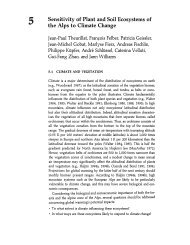
Theor Ecol (2010) 3:97–111<br />
DOI 10.1007/s12080-009-0057-1<br />
ORIGINAL PAPER<br />
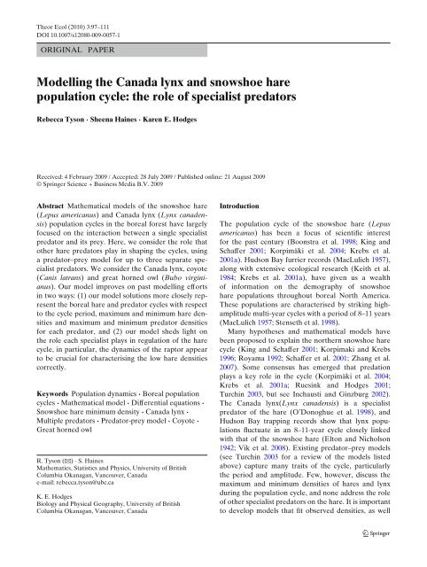
<strong>Modelling</strong> <strong>the</strong> <strong>Canada</strong> <strong>lynx</strong> <strong>and</strong> <strong>snowshoe</strong> <strong>hare</strong><br />
<strong>population</strong> <strong>cycle</strong>: <strong>the</strong> role of specialist predators<br />
Rebecca Tyson · Sheena Haines · Karen E. Hodges<br />
Received: 4 February 2009 / Accepted: 28 July 2009 / Published online: 21 August 2009<br />
© Springer Science + Business Media B.V. 2009<br />
Abstract Ma<strong>the</strong>matical models of <strong>the</strong> <strong>snowshoe</strong> <strong>hare</strong><br />
(Lepus americanus) <strong>and</strong> <strong>Canada</strong> <strong>lynx</strong> (Lynx canadensis)<br />
<strong>population</strong> <strong>cycle</strong>s in <strong>the</strong> boreal forest have largely<br />
focused on <strong>the</strong> interaction between a single specialist<br />
predator <strong>and</strong> its prey. Here, we consider <strong>the</strong> role that<br />
o<strong>the</strong>r <strong>hare</strong> predators play in shaping <strong>the</strong> <strong>cycle</strong>s, using<br />
a predator–prey model for up to three separate specialist<br />
predators. We consider <strong>the</strong> <strong>Canada</strong> <strong>lynx</strong>, coyote<br />
(Canis latrans) <strong>and</strong> great horned owl (Bubo virginianus).<br />
Our model improves on past modelling efforts<br />
in two ways: (1) our model solutions more closely represent<br />
<strong>the</strong> boreal <strong>hare</strong> <strong>and</strong> predator <strong>cycle</strong>s with respect<br />
to <strong>the</strong> <strong>cycle</strong> period, maximum <strong>and</strong> minimum <strong>hare</strong> densities<br />
<strong>and</strong> maximum <strong>and</strong> minimum predator densities<br />
for each predator, <strong>and</strong> (2) our model sheds light on<br />
<strong>the</strong> role each specialist plays in regulation of <strong>the</strong> <strong>hare</strong><br />
<strong>cycle</strong>, in particular, <strong>the</strong> dynamics of <strong>the</strong> raptor appear<br />
to be crucial for characterising <strong>the</strong> low <strong>hare</strong> densities<br />
correctly.<br />
Keywords Population dynamics · Boreal <strong>population</strong><br />
<strong>cycle</strong>s · Ma<strong>the</strong>matical model · Differential equations ·<br />
Snowshoe <strong>hare</strong> minimum density · <strong>Canada</strong> <strong>lynx</strong> ·<br />
Multiple predators · Predator-prey model · Coyote ·<br />
Great horned owl<br />
R. Tyson (B) · S. Haines<br />
Ma<strong>the</strong>matics, Statistics <strong>and</strong> Physics, University of British<br />
Columbia Okanagan, Vancouver, <strong>Canada</strong><br />
e-mail: rebecca.tyson@ubc.ca<br />
K. E. Hodges<br />
Biology <strong>and</strong> Physical Geography, University of British<br />
Columbia Okanagan, Vancouver, <strong>Canada</strong><br />
Introduction<br />
The <strong>population</strong> <strong>cycle</strong> of <strong>the</strong> <strong>snowshoe</strong> <strong>hare</strong> (Lepus<br />
americanus) has been a focus of scientific interest<br />
for <strong>the</strong> past century (Boonstra et al. 1998; King<strong>and</strong><br />
Schaffer 2001; Korpimäki et al. 2004; Krebs et al.<br />
2001a). Hudson Bay furrier records (MacLulich 1957),<br />
along with extensive ecological research (Keith et al.<br />
1984; Krebs et al. 2001a), have given us a wealth<br />
of information on <strong>the</strong> demography of <strong>snowshoe</strong><br />
<strong>hare</strong> <strong>population</strong>s throughout boreal North America.<br />
These <strong>population</strong>s are characterised by striking highamplitude<br />
multi-year <strong>cycle</strong>s with a period of 8–11 years<br />
(MacLulich 1957;Stense<strong>the</strong>tal.1998).<br />
Many hypo<strong>the</strong>ses <strong>and</strong> ma<strong>the</strong>matical models have<br />
been proposed to explain <strong>the</strong> nor<strong>the</strong>rn <strong>snowshoe</strong> <strong>hare</strong><br />
<strong>cycle</strong> (King <strong>and</strong> Schaffer 2001; Korpimaki <strong>and</strong> Krebs<br />
1996; Royama 1992; Schafferetal.2001; Zhang et al.<br />
2007). Some consensus has emerged that predation<br />
plays a key role in <strong>the</strong> <strong>cycle</strong> (Korpimäki et al. 2004;<br />
Krebs et al. 2001a; Ruesink <strong>and</strong> Hodges 2001;<br />
Turchin 2003, but see Inchausti <strong>and</strong> Ginzburg 2002).<br />
The <strong>Canada</strong> <strong>lynx</strong>(Lynx canadensis) is a specialist<br />
predator of <strong>the</strong> <strong>hare</strong> (O’Donoghue et al. 1998), <strong>and</strong><br />
Hudson Bay trapping records show that <strong>lynx</strong> <strong>population</strong>s<br />
fluctuate in an 8–11-year <strong>cycle</strong> closely linked<br />
with that of <strong>the</strong> <strong>snowshoe</strong> <strong>hare</strong> (Elton <strong>and</strong> Nicholson<br />
1942; Vik et al. 2008). Existing predator–prey models<br />
(see Turchin 2003 for a review of <strong>the</strong> models listed<br />
above) capture many traits of <strong>the</strong> <strong>cycle</strong>, particularly<br />
<strong>the</strong> period <strong>and</strong> amplitude. Few, however, discuss <strong>the</strong><br />
maximum <strong>and</strong> minimum densities of <strong>hare</strong>s <strong>and</strong> <strong>lynx</strong><br />
during <strong>the</strong> <strong>population</strong> <strong>cycle</strong>, <strong>and</strong> none address <strong>the</strong> role<br />
of o<strong>the</strong>r specialist predators on <strong>the</strong> <strong>hare</strong>. It is important<br />
to develop models that fit observed densities, as well
98 Theor Ecol (2010) 3:97–111<br />
as <strong>cycle</strong> periods. The low minimum densities have very<br />
real impacts on many species in <strong>the</strong> boreal forest food<br />
web (Ruesink <strong>and</strong> Hodges 2001), so models that do<br />
not capture low densities are failing to describe an<br />
important aspect of <strong>the</strong> <strong>population</strong> <strong>cycle</strong>.<br />
In this paper, we seek to investigate <strong>the</strong>se two omissions<br />
by previous researchers. Since <strong>the</strong> minimum <strong>hare</strong><br />
densities observed in <strong>the</strong> boreal forest are much lower<br />
than existing models predict, we have yet to underst<strong>and</strong><br />
what drives <strong>the</strong> <strong>hare</strong> density to such low values during<br />
<strong>the</strong> <strong>cycle</strong> troughs (Boonstra et al. 1998; Hodges et al.<br />
1999). Predation by <strong>lynx</strong> is apparently not sufficient.<br />
Snowshoe <strong>hare</strong>s, however, are subject to predation by<br />
a myriad of mammalian <strong>and</strong> avian predators (Stenseth<br />
et al. 1997). Fur<strong>the</strong>rmore, <strong>the</strong> Kluane study in <strong>the</strong><br />
Yukon Territory provides data indicating that, in addition<br />
to <strong>the</strong> <strong>lynx</strong>, both <strong>the</strong> coyote (Canis latrans) <strong>and</strong><br />
<strong>the</strong> great horned owl (Bubo virginianis) <strong>population</strong>s<br />
respond to fluctuating <strong>hare</strong> densities as specialist predators<br />
(O’Donoghue et al. 2001; Rohner et al. 2001).<br />
It is thus possible that <strong>the</strong>se predators each play an<br />
important role in shaping <strong>the</strong> dynamics of <strong>the</strong> <strong>hare</strong><br />
<strong>population</strong> <strong>cycle</strong>.<br />
We assess model fit to empirical data through three<br />
<strong>cycle</strong> probes for <strong>the</strong> prey, <strong>and</strong> three <strong>cycle</strong> probes for<br />
each specialist predator: period, <strong>hare</strong> maximum density,<br />
<strong>hare</strong> minimum density <strong>and</strong>, for each specialist<br />
predator, maximum density, minimum density <strong>and</strong> lag.<br />
The predator lag is defined as <strong>the</strong> time between <strong>the</strong><br />
maximum of <strong>the</strong> prey <strong>cycle</strong> <strong>and</strong> <strong>the</strong> subsequent maximum<br />
of <strong>the</strong> predator <strong>cycle</strong>. Using <strong>the</strong>se <strong>cycle</strong> probes,<br />
we address two central questions. First, can a bi-trophic<br />
predator–prey model of <strong>the</strong> <strong>lynx</strong>–<strong>hare</strong> system generate<br />
simulated <strong>cycle</strong>s that match boreal forest <strong>cycle</strong>s if multiple<br />
predators are included? Second, what is <strong>the</strong> role<br />
played by each specialist <strong>hare</strong> predator in <strong>the</strong> <strong>lynx</strong>–<strong>hare</strong><br />
<strong>cycle</strong> dynamics? Our work is a significant extension of<br />
current models, which have concentrated on capturing<br />
<strong>the</strong> qualitative ra<strong>the</strong>r than quantitative behaviour of<br />
<strong>the</strong> <strong>lynx</strong>–<strong>hare</strong> system, <strong>and</strong> which have included only<br />
one specialist predator.<br />
The model<br />
We base our investigation on <strong>the</strong> model used by<br />
Hanski <strong>and</strong> Korpimaki (Hanski <strong>and</strong> Korpimäki 1995)<br />
to analyse vole <strong>population</strong> dynamics in Fennosc<strong>and</strong>ia.<br />
Voles <strong>and</strong> <strong>the</strong>ir predators exhibit distinct 4-year <strong>cycle</strong>s<br />
in <strong>the</strong> nor<strong>the</strong>rn parts of <strong>the</strong> voles’ range. The model<br />
equations are<br />
dN<br />
dt<br />
dP<br />
dt<br />
(<br />
= rN 1 − N )<br />
− γ N2<br />
k N 2 + η − αNP<br />
2 N + μ , (1a)<br />
(<br />
= sP 1 − qP )<br />
, (1b)<br />
N<br />
where N <strong>and</strong> P are <strong>the</strong> prey (vole) <strong>and</strong> specialist<br />
predator <strong>population</strong> density, respectively. We use <strong>the</strong><br />
same model, but with parameters appropriate for <strong>the</strong><br />
<strong>snowshoe</strong> <strong>hare</strong> <strong>and</strong> its predators. We refer to this model<br />
as <strong>the</strong> “basic model”.<br />
Equation 1a has logistic growth of <strong>the</strong> <strong>hare</strong> <strong>population</strong>,<br />
with r <strong>the</strong> <strong>hare</strong>s’ intrinsic rate of <strong>population</strong><br />
growth <strong>and</strong> k <strong>the</strong> carrying capacity. The second term<br />
in <strong>the</strong> prey equation represents predation by generalist<br />
predators, which are assumed to have a sigmoid (type<br />
III) functional response (O’Donoghue et al. 1998). The<br />
parameter γ describes <strong>the</strong> maximum yearly rate of generalist<br />
predation in terms of kills per area, <strong>and</strong> η is <strong>the</strong><br />
<strong>hare</strong> density at which <strong>the</strong> yearly generalist predation<br />
rate is half of γ .ThethirdterminEq.1a reflects specialist<br />
predation on <strong>hare</strong>s. Specialist predators are assumed<br />
to have a type-II functional response (O’Donoghue<br />
et al. 1998; Turchin2003). The three most important<br />
<strong>hare</strong> predators in <strong>the</strong> boreal forest are <strong>the</strong> <strong>lynx</strong>, coyote<br />
<strong>and</strong> great horned owl, <strong>and</strong> <strong>the</strong> functional response of<br />
each of <strong>the</strong>se is well described by <strong>the</strong> type-II response<br />
(Krebs et al. 2001b). The parameter α is <strong>the</strong> maximum<br />
killing rate of <strong>hare</strong>s by specialist predators, <strong>and</strong> μ, <strong>the</strong><br />
half-saturation constant, is <strong>the</strong> <strong>hare</strong> density at which<br />
specialist predation is at half α.<br />
The predator equation (Eq. 1b) consists of a single<br />
logistic growth term with a prey-dependent carrying<br />
capacity, N/q. This formulation of predator dynamics<br />
is analogous to a logistic growth model with variable<br />
predator territories that change in size according to<br />
prey abundance (Turchin 2003). Thus, as <strong>the</strong> <strong>hare</strong><br />
<strong>population</strong> decreases, <strong>the</strong> predator carrying capacity,<br />
N/q, also decreases. The parameter q is <strong>the</strong> equilibrium<br />
density ratio of <strong>hare</strong>s to predators (Turchin <strong>and</strong> Hanski<br />
1997), <strong>and</strong> s is <strong>the</strong> intrinsic rate of increase of <strong>the</strong><br />
predator <strong>population</strong>.<br />
We allowed <strong>the</strong> specialist predator P in Eq. 1 to<br />
represent just <strong>lynx</strong>, or a predator complex of <strong>lynx</strong><br />
<strong>and</strong> o<strong>the</strong>r specialist predators. We considered three<br />
predator complexes: <strong>lynx</strong> <strong>and</strong> coyote (<strong>lynx</strong>:coyote–<strong>hare</strong><br />
system), <strong>lynx</strong> <strong>and</strong> owl (<strong>lynx</strong>:owl–<strong>hare</strong> system) <strong>and</strong> all<br />
three specialists (<strong>lynx</strong>:coyote:owl–<strong>hare</strong> system). Since a<br />
proportion p i of <strong>hare</strong> deaths is due to each predator,
Theor Ecol (2010) 3:97–111 99<br />
we sought to represent <strong>the</strong> combination of specialist<br />
predators as a single combined predator by taking<br />
combined parameter values. The resulting predator parameter<br />
values were weighted sums of <strong>the</strong> individual<br />
parameter values, using <strong>the</strong> predation pressure proportions<br />
p i as <strong>the</strong> weights. For example, if <strong>hare</strong> predation<br />
pressure was due to <strong>lynx</strong>, coyote <strong>and</strong> great horned<br />
owl in <strong>the</strong> ratio p l : p c : p g = 0.6 : 0.3 : 0.1, <strong>the</strong>nα =<br />
(p l α l + p c α c + p g α g ) = 0.6α l + 0.3α c + 0.1α g .Thes, q<br />
<strong>and</strong> μ combination parameters were calculated in <strong>the</strong><br />
same way. We used data on <strong>hare</strong> mortality in <strong>the</strong> boreal<br />
forest as a guideline for plausible p i values.<br />
Additional specialist predators are explicitly included<br />
in <strong>the</strong> model by adding, for each predator, an<br />
equation analogous to Eq. 1b, <strong>and</strong> a separate specialist<br />
predation term in Eq. 1a. The result is <strong>the</strong> following<br />
system of equations:<br />
dN<br />
dt<br />
dP i<br />
dt<br />
= rN<br />
(<br />
1 − N k<br />
)<br />
− γ N2<br />
N 2 + η 2 − ∑ i<br />
α i NP i<br />
N + μ i<br />
,<br />
(2a)<br />
(<br />
= s i P i 1 − q )<br />
i P i<br />
, ∀i. (2b)<br />
N<br />
The index i denotes predator type <strong>and</strong> can be l (<strong>lynx</strong>),<br />
c (coyote) or g (great horned owl).<br />
In any study of model fit to data, it is important to<br />
know how many degrees of freedom are available in<br />
<strong>the</strong> model. To do this here, we must rescale <strong>the</strong> model<br />
variables <strong>and</strong>, <strong>the</strong>reby, uncover <strong>the</strong> relevant dimensionless<br />
parameter groupings. In nondimensional form, <strong>the</strong><br />
model becomes<br />
dn<br />
dt = n(1 − n) − γ ∗ n 2<br />
∗ n 2 + (η ∗ )2 − ∑ i<br />
dp<br />
(<br />
i<br />
dt = ∗ s∗ i p i<br />
1 − p i<br />
n<br />
α i np i<br />
n + μi<br />
∗ , (3a)<br />
)<br />
, ∀i, (3b)<br />
where <strong>the</strong> rescaled variables <strong>and</strong> dimensionless parameter<br />
groupings are<br />
n = N k ,<br />
η ∗ = η k ,<br />
p i = q i P i<br />
k , t∗ = rt, γ ∗ = γ kr ,<br />
α i = α i<br />
q i<br />
,<br />
μ ∗ i = μ i<br />
k ,<br />
s∗ i = s i<br />
r .<br />
The prey equation (Eq. 3a) has two generalist predation<br />
parameters, plus two parameters for each specialist<br />
predator. The predator equations (Eq. 3b) each have<br />
just one parameter.<br />
Below, we investigate models with one, two <strong>and</strong><br />
three specialist predators, using parameter values from<br />
field research. The multiple predator models we consider<br />
are:<br />
• The LC model: <strong>lynx</strong>, coyote, <strong>snowshoe</strong> <strong>hare</strong><br />
• The LG model: <strong>lynx</strong>, great horned owl, <strong>snowshoe</strong><br />
<strong>hare</strong><br />
• The LCG model: <strong>lynx</strong>, coyote, great horned owl,<br />
<strong>snowshoe</strong> <strong>hare</strong><br />
Parameter estimation<br />
The parameter values we used (Table 1) were chosen<br />
based on field studies, primarily from <strong>the</strong> comprehensive<br />
ecosystem study at Kluane Lake, Yukon (Krebs<br />
et al. 2001b), which included several different study<br />
sites. Snowshoe <strong>hare</strong> densities at each site were estimated<br />
by mark-recapture live-trapping, thus providing<br />
high-quality estimates of <strong>hare</strong> densities in this system.<br />
We supplemented <strong>the</strong>se values with data from o<strong>the</strong>r<br />
sources if parameters were not well estimated by <strong>the</strong><br />
Kluane study or if o<strong>the</strong>r studies showed widely divergent<br />
values, indicating that model behaviour should<br />
be tested over a broad range. Below, we outline how<br />
<strong>the</strong> various parameter values were determined in <strong>the</strong><br />
literature.<br />
Intrinsic rate of <strong>population</strong> increase values were<br />
determined from direct measurements of <strong>population</strong><br />
increase (r) or from annual litter size data (ρ) coupled<br />
with survival rates of <strong>the</strong> young (δ). Given ρ <strong>and</strong> δ,<br />
<strong>the</strong> corresponding annual rate of <strong>population</strong> increase<br />
is determined from<br />
r = ln(ρδ).<br />
The <strong>snowshoe</strong> <strong>hare</strong> carrying capacity (k) is estimated<br />
from observations of maximum <strong>hare</strong> densities observed<br />
in <strong>the</strong> field. The generalist predation rate (γ ) has been<br />
measured on control grids in Kluane. The generalist<br />
half-saturation constant (η) cannot be directly measured<br />
in <strong>the</strong> field, <strong>and</strong> so we use a range of values. We<br />
selected a plausible range by using measured values for<br />
specialist predator half-saturation constants (μ) fora<br />
variety of predators as a guideline.<br />
Predator half-saturation constants (μ i ) are determined<br />
from functional response curves fitted to predation<br />
data plotted as a function of prey density. Maximal<br />
daily kill rates (α i ) are estimated from field data <strong>and</strong><br />
from functional response curves. These values are <strong>the</strong>n<br />
multiplied by 365 days/year to give <strong>the</strong> yearly saturation<br />
killing rate.
100 Theor Ecol (2010) 3:97–111<br />
Table 1 Parameters for <strong>the</strong> model equations Eqs. 1 <strong>and</strong> 2<br />
Description (units) Source Range Default value<br />
Basic model<br />
r Hare intrinsic rate of increase (/yr) (a)(f) 1.5–2.0 8.0 5.0<br />
k Hare carrying capacity (<strong>hare</strong>s/ha) (a)(e) 4.0–8.0 (12) 1.75 1.75<br />
γ Generalist killing rate (<strong>hare</strong>s/(ha·yr)) (a) 0.1–2.0 0.1 0.1<br />
η Generalist half-saturation constant (<strong>hare</strong>s/ha) 0.5–2.0 1.25 1.25<br />
α l Lynx saturation killing rate (<strong>hare</strong>s/(<strong>lynx</strong>·yr)) (b)(d) 438–577 505 505<br />
α c Coyote saturation killing rate (<strong>hare</strong>s/(coyote·yr)) (b)(d) 840–876 – 858<br />
α g Great horned owl saturation killing rate (<strong>hare</strong>s/(owl·yr)) (c) 50–150 (250) – 100<br />
μ l Lynx half-saturation constant (<strong>hare</strong>s/ha) (d) 0.2–0.4 0.3 0.3<br />
μ c Coyote half-saturation constant (<strong>hare</strong>s/ha) (d) 0.5–1.1 – 0.8<br />
μ g Great horned owl half-saturation constant (<strong>hare</strong>s/ha) (c) 0.05–0.25 – 0.15<br />
s l Lynx rate of <strong>population</strong> increase (/yr) (e)(f) 0.7–1.0 0.85 0.8<br />
s c Coyote rate of <strong>population</strong> increase (/yr) (f)(g) 0.5–1.2 – 0.55<br />
s g Great horned owl rate of <strong>population</strong> increase (/yr) (c) 0.2–0.5 – 0.35<br />
q l Hare:<strong>lynx</strong> equilibrium ratio (<strong>hare</strong>s/<strong>lynx</strong>) (b) 150–1200 212 500<br />
q c Hare:coyote equilibrium ratio (<strong>hare</strong>s/coyote) (b) 330–2500 – 1075<br />
q g Hare:great horned owl equilibrium ratio (<strong>hare</strong>s/owl) (c) 50–250 – 100<br />
LCG model<br />
Parameters values derived from <strong>the</strong> data (column 4) are measured or calculated as described in “Parameter estimation”. Default<br />
parameter values for <strong>the</strong> basic <strong>and</strong> LCG (columns 5 <strong>and</strong> 6) models are chosen midway through <strong>the</strong> observed range except in cases<br />
where <strong>the</strong> model solutions did not <strong>cycle</strong>. For <strong>the</strong> basic model, <strong>the</strong>refore, it was necessary to set k <strong>and</strong> q l at <strong>the</strong> extreme low <strong>and</strong> high<br />
end of <strong>the</strong> observed ranges, respectively. Sources are Hodges et al. (2001) (a), O’Donoghue et al. (2001) (b), Rohner et al. (2001) (c),<br />
O’Donoghue et al. (1998) (d), Ruggerio et al. (2000) (e), King <strong>and</strong> Schaffer (2001) (f) <strong>and</strong> Windberg (1995) (g)<br />
The <strong>hare</strong>:predator equilibrium ratio q i determines<br />
<strong>the</strong> carrying capacity of <strong>the</strong> environment for <strong>the</strong> predator,<br />
<strong>and</strong> is very difficult to estimate with certainty.<br />
The ratio can be calculated using predator energetic<br />
needs (prey/predator/year), or from demographic data.<br />
Generally, estimates derived from energetic needs are<br />
two to three times lower than estimates derived from<br />
demographic data, <strong>and</strong> so <strong>the</strong> plausible range of values<br />
is relatively large compared to <strong>the</strong> o<strong>the</strong>r parameters of<br />
<strong>the</strong> model.<br />
Model analysis<br />
It is not possible to determine <strong>the</strong> characteristics of <strong>the</strong><br />
limit <strong>cycle</strong> solutions to our models analytically, <strong>and</strong> so<br />
we carried out a numerical study. Each parameter was<br />
varied through <strong>the</strong> range of biologically realistic values<br />
from boreal North America (Table 1), <strong>and</strong> for some<br />
of <strong>the</strong> parameters, we also investigated values outside<br />
<strong>the</strong> realistic range in order to better underst<strong>and</strong> <strong>the</strong><br />
solution behaviour.<br />
For each set of parameter values, we obtained numerical<br />
solutions to <strong>the</strong> model equations using a fourthorder<br />
Runge Kutta scheme. Numerical solutions were<br />
run for 600 years, <strong>and</strong> <strong>the</strong>n <strong>the</strong> first 500 were discarded<br />
so that transient behaviour was not included in our<br />
analysis. In every case, <strong>the</strong> steady state behaviour for N<br />
<strong>and</strong> P i was ei<strong>the</strong>r a limit <strong>cycle</strong> or a constant equilibrium.<br />
The period, maximum <strong>population</strong> density <strong>and</strong> minimum<br />
<strong>population</strong> density of <strong>the</strong> cyclic solutions for N<br />
<strong>and</strong> P i were measured from <strong>the</strong> numerical time series.<br />
These probes were <strong>the</strong>n compared to field data.<br />
We explored a wide range <strong>and</strong> combination of parameter<br />
values in our investigations. For <strong>the</strong> discussion<br />
below, we found it useful to choose default parameter<br />
values in <strong>the</strong> middle of each plausible parameter range<br />
(Table 1). The two exceptions to this rule are k <strong>and</strong> q l in<br />
<strong>the</strong> basic model, which had to be chosen at <strong>the</strong> extreme<br />
high <strong>and</strong> low end of <strong>the</strong> plausible range, respectively, in<br />
order for <strong>the</strong> default parameter set to yield <strong>population</strong><br />
<strong>cycle</strong>s in <strong>the</strong> solutions. We used <strong>the</strong> model solutions<br />
obtained with <strong>the</strong>se default values as a starting point<br />
to examine how <strong>the</strong> <strong>cycle</strong> characteristics of <strong>the</strong> model<br />
solutions depended on variations in <strong>the</strong> model parameters.<br />
Parameter sensitivity<br />
We investigated <strong>the</strong> sensitivity of <strong>the</strong> model solutions<br />
to variation in individual model parameters, <strong>and</strong> also<br />
did some work in which we varied multiple parameters<br />
simultaneously. Changes in <strong>the</strong> numerically generated<br />
time series were observed with respect to <strong>the</strong> <strong>cycle</strong><br />
probes identified in “Introduction”. Results for <strong>the</strong><br />
basic <strong>and</strong> LCG models are shown in Fig. 1. In<strong>the</strong><br />
interest of brevity, <strong>the</strong> figure shows <strong>the</strong> sensitivity of<br />
just two <strong>cycle</strong> probes, <strong>hare</strong> maxima <strong>and</strong> minima, to
Theor Ecol (2010) 3:97–111 101<br />
Fig. 1 Sensitivity of <strong>the</strong> <strong>hare</strong> minimum <strong>and</strong> maximum densities<br />
to model parameters. Results are shown for <strong>the</strong> a basic <strong>and</strong> b<br />
LCG models. Model behaviour was tested for all parameters held<br />
at <strong>the</strong>ir default values (Table 1, except for <strong>the</strong> one parameter<br />
being varied. The grey rectangles show <strong>the</strong> range of observed<br />
low <strong>and</strong> high densities across several sites in <strong>the</strong> Yukon. Ranges<br />
over which each parameter was varied are listed on <strong>the</strong> vertical<br />
axis, across from <strong>the</strong> corresponding <strong>cycle</strong> response ranges. The<br />
parameter ranges correspond to <strong>the</strong> range of plausible values for<br />
each parameter (see Table 1), except in cases where <strong>the</strong> model<br />
did not yield <strong>cycle</strong>s for parameter values at ei<strong>the</strong>r end of <strong>the</strong><br />
range. Solutions with <strong>cycle</strong> amplitude (maximum density divided<br />
by minimum density) of less than 1.5 were deemed non-cyclic,<br />
since <strong>cycle</strong>s of such low amplitude would be difficult to detect<br />
in <strong>the</strong> field, given <strong>the</strong> individual confidence limits around each<br />
density estimate<br />
individual parameter variations when all o<strong>the</strong>r parameters<br />
are held constant at <strong>the</strong> default values (Table 1).<br />
The corresponding <strong>cycle</strong> periods showed relatively little<br />
sensitivity to variations in parameter values, remaining<br />
generally within <strong>the</strong> plausible range of values. Cycle<br />
periods generally fell within <strong>the</strong> range of 8–9 years for<br />
<strong>the</strong> basic model, <strong>and</strong> 9–12 years for <strong>the</strong> LCG model.<br />
Similar sensitivity results were obtained for model parameters<br />
fixed at o<strong>the</strong>r plausible values. Below, we<br />
describe <strong>the</strong> full response of <strong>the</strong> model solutions, in<br />
terms of all of <strong>the</strong> <strong>cycle</strong> probes, to variations in <strong>the</strong><br />
model parameters.<br />
All of <strong>the</strong> models gave rise to periodic limit <strong>cycle</strong><br />
oscillations for a wide range of parameter values.<br />
Figures 2 <strong>and</strong> 3 show sample <strong>population</strong> density time<br />
series from <strong>the</strong> basic <strong>and</strong> LCG models obtained with<br />
default parameter values (<strong>the</strong> default values are listed<br />
in Fig. 1). Consistent with time series from <strong>the</strong> boreal<br />
forest, <strong>the</strong> predator <strong>cycle</strong>s lag 1–2 years behind <strong>the</strong> <strong>hare</strong><br />
<strong>cycle</strong>.<br />
Hanski <strong>and</strong> Korpimäki (1995) analysed <strong>the</strong> basic<br />
model of Eq. 1a in parameter ranges appropriate for<br />
<strong>the</strong> vole food web, <strong>and</strong> found that parameters r, s, k<br />
<strong>and</strong> μ had <strong>the</strong> strongest influence on model dynamics.<br />
Using values appropriate for <strong>the</strong> <strong>Canada</strong> <strong>lynx</strong> <strong>and</strong><br />
<strong>snowshoe</strong> <strong>hare</strong>, we also found that <strong>the</strong>se parameters are<br />
important (Fig. 1-A). The parameters r <strong>and</strong> s (intrinsic<br />
rate of <strong>hare</strong> <strong>and</strong> predator <strong>population</strong> increase) have<br />
<strong>the</strong> strongest influence on <strong>cycle</strong> length, with low values<br />
increasing <strong>the</strong> <strong>cycle</strong> period to 10–11 years, <strong>and</strong> higher<br />
values decreasing <strong>the</strong> <strong>cycle</strong> period to 7–9 years. These<br />
parameters also affect predator lag, with lag decreasing<br />
with increasing s or decreasing r. Parameter k (<strong>hare</strong>carrying<br />
capacity) has a strong effect on <strong>cycle</strong> amplitude,<br />
with increasing values increasing peak densities<br />
significantly while increasing low densities only slightly.<br />
The parameter μ (predator half-saturation constant)<br />
has strong effects on <strong>the</strong> model dynamics, as small<br />
decreases in μ significantly affect <strong>cycle</strong> amplitude, both<br />
increasing peak densities <strong>and</strong> lowering low densities.<br />
For <strong>the</strong> default values of <strong>the</strong>se four parameters, <strong>the</strong><br />
model always predicts stable limit <strong>cycle</strong>s. In contrast,<br />
at low values for r <strong>and</strong> k <strong>and</strong> at high values for s <strong>and</strong> μ,<br />
<strong>the</strong> limit <strong>cycle</strong> collapses to a stable equilibrium point.<br />
The <strong>hare</strong>:predator equilibrium ratio, q, also has important<br />
effects on <strong>the</strong> model dynamics. Additionally, q<br />
is <strong>the</strong> most difficult parameter to estimate, <strong>and</strong> so sensitivity<br />
of <strong>the</strong> model to changes in q is highly relevant. For<br />
<strong>the</strong> basic model, q has little effect on <strong>cycle</strong> period <strong>and</strong><br />
only a minor effect on <strong>cycle</strong> amplitude, but it is <strong>the</strong> most<br />
important parameter in shifting <strong>the</strong> model from a stable<br />
equilibrium point to a stable limit <strong>cycle</strong>. The range of<br />
values for which <strong>the</strong> model exhibits stable limit <strong>cycle</strong>s<br />
is small relative to <strong>the</strong> range of plausible values for q
102 Theor Ecol (2010) 3:97–111<br />
3<br />
2<br />
A<br />
1<br />
0<br />
0 5 10 15 20 25 30 35 40 45 50<br />
time (years)<br />
8 x 10⁻³ time (years)<br />
6<br />
B<br />
4<br />
2<br />
0<br />
0 5 10 15 20 25 30 35 40 45 50<br />
C<br />
time (years)<br />
Fig. 2 Sample time series for <strong>the</strong> basic model. The <strong>hare</strong> <strong>and</strong><br />
<strong>lynx</strong> time series are shown separately in a <strong>and</strong> b, respectively,<br />
<strong>and</strong> toge<strong>the</strong>r in c. The <strong>hare</strong> <strong>and</strong> <strong>lynx</strong> <strong>population</strong> densities are<br />
normalised in c to lie between 0 <strong>and</strong> 1 so that <strong>the</strong> two time<br />
series can be easily viewed toge<strong>the</strong>r, showing <strong>the</strong> predator lag.<br />
Parameter values are: r = 1.75, k = 8, γ = 0.1, η = 1.25, α = 505,<br />
μ = 0.3, s = 0.85 <strong>and</strong> q = 212<br />
(Fig. 4); for all predator combinations investigated, <strong>the</strong><br />
largest range of q values that evinces <strong>cycle</strong>s is 125–300<br />
<strong>hare</strong>s/predator, <strong>and</strong> most combinations only <strong>cycle</strong>d for<br />
q within 150–275 <strong>hare</strong>s/predator.<br />
In <strong>the</strong> multiple-predator LC, LG <strong>and</strong> LCG models,<br />
<strong>the</strong> parameters r, k, s i <strong>and</strong> μ i all have similar effects<br />
on model dynamics as <strong>the</strong>y do in <strong>the</strong> single predator<br />
model (sensitivity results for <strong>the</strong> LCG model are shown<br />
in Fig. 1b; results for <strong>the</strong> LC <strong>and</strong> LG models are not<br />
shown). The model solutions respond differently, however,<br />
to changes in <strong>the</strong> parameters q i . Increasing any of<br />
<strong>the</strong> three <strong>hare</strong>:predator equilibrium ratios, q i ,to<strong>the</strong>ir<br />
maximum values increased <strong>the</strong> <strong>cycle</strong> period, as in <strong>the</strong><br />
basic model, but beyond this simple relationship, <strong>the</strong><br />
three parameters affected <strong>the</strong> model in quite different<br />
ways. The <strong>hare</strong>:<strong>lynx</strong> ratio q l is <strong>the</strong> only ratio that affected<br />
<strong>the</strong> stability of <strong>the</strong> model. The lowest estimated<br />
values for q l led to stable equilibrium solutions in all<br />
of <strong>the</strong> multiple-predator models. In contrast, q c <strong>and</strong> q g<br />
had little to no effect on <strong>the</strong> existence of limit <strong>cycle</strong><br />
solutions, but did affect <strong>cycle</strong> amplitude. Increasing<br />
ei<strong>the</strong>r q c or q g reduced <strong>cycle</strong> amplitude, with q g having<br />
a much stronger effect than q c . Between <strong>the</strong> default <strong>and</strong><br />
maximum values for q g , <strong>the</strong> <strong>cycle</strong> amplitude increased<br />
tenfold.<br />
Comparison of model solutions to field data<br />
The performance of each model with respect to <strong>the</strong> boreal<br />
<strong>cycle</strong>s at Kluane Lake, Yukon Territory, described<br />
by Krebs et al. (2001b), is summarised in Table 2. For<br />
each model <strong>and</strong> realistic parameter values, we show <strong>the</strong><br />
best match to <strong>the</strong> data that we were able to obtain. A<br />
match was recorded if <strong>the</strong> probe values from <strong>the</strong> simulated<br />
time series fell within <strong>the</strong> range for <strong>the</strong> natural<br />
boreal time series. The LCG model came closest to a
Theor Ecol (2010) 3:97–111 103<br />
4<br />
2<br />
A<br />
0<br />
0 5 10 15 20 25 30 35 40 45 50<br />
4 x 10⁻³<br />
B<br />
2<br />
0<br />
0 5 10 15 20 25 30 35 40 45 50<br />
2 x 10- 3<br />
C<br />
1<br />
0<br />
0 5 10 15 20 25 30 35 40 45 50<br />
0.01<br />
0.005<br />
D<br />
0<br />
0 5 10 15 20 25 30 35 40 45 50<br />
E<br />
time (years)<br />
Fig. 3 Sample time series for <strong>the</strong> LCG model. The <strong>hare</strong>, <strong>lynx</strong>,<br />
coyote <strong>and</strong> great horned owl times series are shown separately<br />
in a–d, in that order, <strong>and</strong> toge<strong>the</strong>r in e. The <strong>hare</strong> <strong>and</strong> predator<br />
<strong>population</strong>s are each normalised in e to lie between 0 <strong>and</strong> 1 so<br />
that <strong>the</strong> four time series can be easily viewed toge<strong>the</strong>r, showing<br />
<strong>the</strong> separate predator lags. Parameter values are: r = 1.75, k = 5,<br />
η = 1.25, α l = 505, μ l = 0.3, s l = 0.85, q l = 700, α c = 858, μ c =<br />
0.8, s c = 0.55, q c = 1075, α g = 100, μ g = 0.15, s g = 0.35 <strong>and</strong> q g =<br />
100<br />
satisfactory match to <strong>the</strong> data. We discuss <strong>the</strong> fit of each<br />
individual model below.<br />
The basic model<br />
For <strong>the</strong> basic model, we found that, with a single predator,<br />
<strong>the</strong> model can capture <strong>cycle</strong> period, predator lag<br />
<strong>and</strong> maximum <strong>hare</strong> densities, but fails to accurately<br />
describe minimum <strong>hare</strong> densities or predator densities<br />
at ei<strong>the</strong>r <strong>the</strong> maximum or minimum of <strong>the</strong> <strong>cycle</strong>. As<br />
described in “The model”, <strong>the</strong> single predator was<br />
ei<strong>the</strong>r <strong>lynx</strong> or a predator complex of <strong>lynx</strong> with one or<br />
two o<strong>the</strong>r specialist predators. The best match to boreal<br />
<strong>cycle</strong>s was obtained with <strong>the</strong> <strong>lynx</strong>:owl–<strong>hare</strong> system but,<br />
though predicted <strong>hare</strong> minimum densities were lower<br />
than in ei<strong>the</strong>r of <strong>the</strong> o<strong>the</strong>r two systems, <strong>the</strong> simulated<br />
<strong>cycle</strong>s could still only match <strong>cycle</strong> period <strong>and</strong> predator<br />
lag.<br />
To obtain cyclic behaviour in <strong>the</strong> model solutions,<br />
it was necessary to keep q values within <strong>the</strong> low end<br />
of <strong>the</strong> tested range. Doing so, however, resulted in<br />
higher predator densities. For <strong>the</strong> <strong>lynx</strong>–<strong>hare</strong> model, it<br />
appears that, for <strong>lynx</strong> alone to exert sufficient predation<br />
pressure on <strong>the</strong> <strong>hare</strong> to cause <strong>population</strong> <strong>cycle</strong>s at all,<br />
<strong>the</strong> <strong>population</strong> densities of <strong>lynx</strong> would have to be well<br />
above any that have been recorded throughout North<br />
America.<br />
The LC <strong>and</strong> LG models<br />
Consistent with our results for <strong>the</strong> basic model, we<br />
found that predator–prey <strong>cycle</strong>s can occur with only <strong>the</strong><br />
mammalian predators included—<strong>lynx</strong> <strong>and</strong> coyote (LC<br />
model)—but that <strong>hare</strong> <strong>population</strong> densities during <strong>the</strong><br />
low phase still remain well above <strong>the</strong>ir observed densities.<br />
As with <strong>the</strong> basic model, <strong>cycle</strong>s are predicted only
104 Theor Ecol (2010) 3:97–111<br />
3<br />
2.5<br />
2<br />
1.5<br />
1<br />
0.5<br />
0<br />
50 100 150 200 250 300 350 400<br />
Fig. 4 Bifurcation plot showing <strong>the</strong> maximum (solid curve) <strong>and</strong><br />
minimum (dotted curve) <strong>hare</strong> <strong>population</strong>s from <strong>the</strong> basic model<br />
of Eq. 1a as functions of <strong>the</strong> <strong>hare</strong>:predator equilibrium ratio q.<br />
When <strong>the</strong> two curves coalesce, <strong>the</strong> maximum <strong>and</strong> minimum are<br />
equal <strong>and</strong> <strong>the</strong> <strong>hare</strong> <strong>population</strong> is not cycling. The values of <strong>the</strong><br />
o<strong>the</strong>r parameters are r = 1.75, k = 8, γ = 0.1, η = 1.25, α = 505,<br />
μ = 0.3 <strong>and</strong> s = 0.85<br />
for <strong>the</strong> lowest range of <strong>hare</strong>:predator ratios, q i .This<br />
result means that, as with <strong>the</strong> basic model, predator<br />
densities remain well above those observed at Kluane.<br />
In <strong>the</strong> two predator models, we found that <strong>the</strong> range<br />
of parameter values for which <strong>the</strong> model showed <strong>cycle</strong>s<br />
was larger than for any predator complex in <strong>the</strong><br />
single-predator models. In particular, we found that<br />
we use a much wider range of plausible values for <strong>the</strong><br />
<strong>hare</strong>:predator equilibrium ratios (q i ), <strong>and</strong> still obtain<br />
cyclic solution behaviour. Predator numbers, however,<br />
were still not fully in line with Kluane <strong>population</strong> densities.<br />
When we analysed <strong>the</strong> model with <strong>lynx</strong> <strong>and</strong> great<br />
horned owl as <strong>the</strong> two specialist predators (LG model),<br />
predicted dynamics were quite different from those discussed<br />
thus far. Hare densities at all phases of <strong>the</strong> <strong>cycle</strong><br />
were in much closer agreement with observed densities,<br />
which seems to be a result of <strong>the</strong> much lower halfsaturation<br />
constant for great horned owl predation, μ g .<br />
Great horned owl densities were in fairly close agreement<br />
with <strong>the</strong> Kluane data, but <strong>lynx</strong> densities could not<br />
be brought down to a plausible range of values.<br />
Table 2 Summary of model fit to <strong>the</strong> <strong>cycle</strong> probes<br />
Probe Data a Basic model LC & LG models LCG model<br />
l l:c l:g l:c:g l&c l&g l,c&g<br />
√ √<br />
√ √ √ √<br />
Hare density (/ha) max 1.5–2.9<br />
×<br />
√<br />
min 0.08–0.16 × × × × × ×<br />
Pred. complex density (/100 km 2 √<br />
) max varies – × ×<br />
– – –<br />
√<br />
min varies – × ×<br />
– – –<br />
Lynx density (/100 km 2 √<br />
) max 30–45 × – – – × ×<br />
√<br />
min 0–3 × – – – × ×<br />
Coyote density (/100 km 2 ) max 9–30 b √<br />
– – – – × –<br />
min 1–5 b √<br />
– – – – × –<br />
Owl density (/100 km 2 ) max 90 c √<br />
√<br />
– – – – –<br />
min 20 c √<br />
√<br />
– – – – –<br />
√ √ √ √ √ √ √<br />
Predator lag (years) l 1–2<br />
√<br />
√<br />
c 1–2 – – – –<br />
–<br />
√<br />
√<br />
g 1–2 – – – – –<br />
√ √ √ √ √ √ √<br />
Period (years) 9–11<br />
Performance<br />
# Dimensionless model parameters 5 5 5 5 8 8 11<br />
# Probes to match 6 6 6 6 9 9 12<br />
# Matched 3 3 2 5 5 7 12<br />
Predators are denoted l (<strong>lynx</strong>), c (coyote) <strong>and</strong> g (great horned owl). Where predators are combined in a complex, <strong>the</strong> appropriate<br />
minimum <strong>and</strong> maximum predator densities are <strong>the</strong> sum of <strong>the</strong> individual maximum <strong>and</strong> minimum densities for each included species.<br />
A √ (×) appears in <strong>the</strong> table where simulation values fell inside (outside) <strong>the</strong> acceptable range defined by <strong>the</strong> data. A dash indicates<br />
that <strong>the</strong> probe was not available for that model<br />
a All data values were obtained from Kluane (Krebs et al. 2001a; Boutin et al. 1995), except as noted below. The ranges of values ei<strong>the</strong>r<br />
reflect different study areas (e.g., <strong>hare</strong> density) or <strong>the</strong> uncertainty around estimates (e.g., maximum <strong>lynx</strong> densities)<br />
b Coyote density values from Kluane were supplemented with data from central Alberta (Nellis <strong>and</strong> Keith 1976) <strong>and</strong> eastern <strong>Canada</strong><br />
(Dumont et al. 2000; Mosnier et al. 2008; Patterson <strong>and</strong> Messier 2001)<br />
c It was not possible to determine data ranges for <strong>the</strong> great horned owl density, <strong>and</strong> so, only <strong>the</strong> single values measured at Kluane<br />
are reported. We accepted simulation time series as fitting <strong>the</strong> great horned owl data if <strong>the</strong> maximum values fell within 30% of <strong>the</strong><br />
observed value, <strong>and</strong> if <strong>the</strong> minimum values fell within 10% of <strong>the</strong> observed value. These ranges are consistent, or more restrictive, than<br />
<strong>the</strong> observed ranges for <strong>the</strong> <strong>hare</strong>s <strong>and</strong> o<strong>the</strong>r predators
Theor Ecol (2010) 3:97–111 105<br />
The LCG model<br />
The most striking difference between <strong>the</strong> LCG model<br />
<strong>and</strong> all of <strong>the</strong> o<strong>the</strong>r models is <strong>the</strong> effect of <strong>the</strong><br />
<strong>hare</strong>:predator ratios, q v . In <strong>the</strong> bifurcation plots (Fig. 5),<br />
we set all parameters at <strong>the</strong> default values given in<br />
Table 1 <strong>and</strong> explored how each ratio (q l , q c <strong>and</strong> q g )<br />
affected <strong>the</strong> model dynamics. Limit <strong>cycle</strong> solutions are<br />
obtained for a much larger range of values than can be<br />
used for q or q i in any of <strong>the</strong> o<strong>the</strong>r models. In contrast,<br />
if we use <strong>the</strong> estimated <strong>hare</strong>:predator ratios that give<br />
<strong>cycle</strong>s in <strong>the</strong> basic model (150–250 <strong>hare</strong>s/predator, with<br />
<strong>the</strong> predator being ei<strong>the</strong>r one species or a predator<br />
complex), <strong>the</strong> LCG model converges to a stable equilibrium<br />
point.<br />
The estimated ranges for <strong>the</strong> q v parameters are<br />
quite large (see Table 1), especially for <strong>the</strong> <strong>lynx</strong> <strong>and</strong><br />
coyote. As mentioned in “Parameter estimation”, <strong>the</strong><br />
lower bounds are determined from calculations based<br />
on energetic needs, while <strong>the</strong> upper bounds are based<br />
on observed <strong>population</strong> densities. In <strong>the</strong> LCG model,<br />
<strong>the</strong> larger values of q v yield <strong>cycle</strong>s of approximately<br />
9–10 years, with predator densities <strong>and</strong> <strong>cycle</strong> lags of<br />
1–2 years, consistent with field observations (Krebs<br />
et al. 2001a).<br />
An exhaustive search through parameter space was<br />
not possible, due to <strong>the</strong> large number of parameters,<br />
but we found a number of different parameter sets for<br />
which <strong>the</strong> model solutions provided a satisfactory fit to<br />
<strong>the</strong>data(Table3). In particular, with <strong>the</strong> LCG model,<br />
3<br />
3<br />
2<br />
2<br />
1<br />
1<br />
0<br />
0 500 1200 1500<br />
ql (<strong>hare</strong>s/<strong>lynx</strong>)<br />
(a) q l bifurcation plot<br />
0<br />
200 800 1400 2000<br />
q c (<strong>hare</strong>s/coyote)<br />
(b) q c bifurcation plot<br />
4<br />
3<br />
2<br />
1<br />
0<br />
100<br />
200 300<br />
400<br />
q g (<strong>hare</strong>s/owl)<br />
(b) q g bifurcation plot<br />
Fig. 5 Bifurcation plots for <strong>the</strong> LCG model showing <strong>the</strong> maximum<br />
(solid curve) <strong>and</strong> minimum (dotted curve) <strong>hare</strong> densities<br />
as functions of q l , q c or q g . When <strong>the</strong> two curves coalesce, <strong>the</strong><br />
maximum <strong>and</strong> minimum are equal <strong>and</strong> <strong>the</strong> <strong>hare</strong> <strong>population</strong> is<br />
not cycling. When not being varied, q l , q c <strong>and</strong> q g were held at<br />
700, 1,075 <strong>and</strong> 100, respectively. All o<strong>the</strong>r parameter values were<br />
r = 1.75, k = 5, γ = 0.1, η = 1.25, α l = 505, μ l = 0.3, α c = 858,<br />
μ c = 0.8, α g = 100, μ g = 0.15, s l = 0.85, s c = 0.55 <strong>and</strong> s g = 0.35.<br />
a q l bifurcation plot, b q c bifurcation plot <strong>and</strong> c q g bifurcation<br />
plot
106 Theor Ecol (2010) 3:97–111<br />
Table 3 We found a number of parameter sets for which <strong>the</strong> LCG model yielded solutions with <strong>cycle</strong> probes that produced a<br />
satisfactory match to <strong>the</strong> data<br />
Source Data a LCG model<br />
Parameter set 1 Parameter set 2<br />
Hare density (/ha) max 1.5–2.9 2.4 2.2<br />
min 0.08–0.16 0.11 0.17<br />
Lynx density (/100 km 2 ) max 30–45 37 25<br />
min 0–3 3 3<br />
Coyote density (/100 km 2 ) max 9–30 b 14 28<br />
min 1–5 b 2.0 5<br />
Owl density (/100 km 2 ) max 90 c 110 65<br />
min 20 c 19 21<br />
Predator lag (years) <strong>lynx</strong> 1–2 1.2 1.2<br />
coyote 1-2 1.7 1.6<br />
owl 1–2 1.9 2.1<br />
Period (years) 9–11 9.5 9.7<br />
The probe values from two such parameter sets are shown. The model parameter values are as reported in Fig. 6 (parameter set 1) <strong>and</strong><br />
Fig. 7 (parameter set 2)<br />
a All data values were obtained from Kluane (Krebs et al. 2001a; Boutin et al. 1995), except as noted below<br />
b Coyote density values from Kluane were supplemented with data from central Alberta (Nellis <strong>and</strong> Keith 1976) <strong>and</strong> eastern <strong>Canada</strong><br />
(Dumont et al. 2000; Mosnier et al. 2008; Patterson <strong>and</strong> Messier 2001)<br />
( c )It was not possible to determine data ranges for <strong>the</strong> great horned owl density, <strong>and</strong> so, only <strong>the</strong> single values measured at Kluane<br />
are reported. For <strong>the</strong>se cases, we accepted simulation time series as fitting <strong>the</strong> great horned owl data if <strong>the</strong> maximum values fell within<br />
30% of <strong>the</strong> observed value, <strong>and</strong> if <strong>the</strong> minimum values fell within 10% of <strong>the</strong> observed value. These ranges are consistent with, or more<br />
restrictive than, <strong>the</strong> observed ranges for <strong>the</strong> <strong>hare</strong>s <strong>and</strong> o<strong>the</strong>r predators<br />
it was finally possible to match <strong>the</strong> <strong>hare</strong> minimum densities,<br />
while still keeping predator numbers inside a reasonable<br />
range. The fits to <strong>cycle</strong> probes corresponding<br />
to two such parameter sets are shown in Table 3.These<br />
two parameter sets are quite different, <strong>and</strong> illustrate <strong>the</strong><br />
type of cyclic behaviour that can be obtained with <strong>the</strong><br />
LCG model.<br />
The role of each specialist predator<br />
The LCG model allows us to explore <strong>the</strong> different effects<br />
of predation by <strong>lynx</strong>, coyote <strong>and</strong> great horned owl.<br />
Using <strong>the</strong> parameter values identified in “Parameter<br />
estimation”, our model predicts that great horned owl<br />
predation is particularly important. While <strong>the</strong> <strong>lynx</strong> <strong>and</strong><br />
coyote predation parameters have relatively minor effects<br />
on <strong>cycle</strong> amplitude <strong>and</strong> period, <strong>the</strong> parameters<br />
relating to great horned owl predation are much more<br />
significant. This result can be explained in terms of<br />
<strong>the</strong> magnitude of great horned owl predation at low<br />
prey densities. The predation characteristics of <strong>the</strong><br />
great horned owl, as captured in <strong>the</strong> parameters α g<br />
<strong>and</strong> μ g , are very different from those of <strong>the</strong> o<strong>the</strong>r two<br />
specialist predators. The saturation killing rate (α g )is<br />
significantly lower than that of ei<strong>the</strong>r <strong>the</strong> <strong>lynx</strong> or <strong>the</strong><br />
coyote. This means that, at high <strong>hare</strong> densities, great<br />
horned owls cause less <strong>hare</strong> mortality, per capita, than<br />
ei<strong>the</strong>r <strong>lynx</strong> or coyotes. The much higher <strong>population</strong><br />
of great horned owls, however, counteracts this effect.<br />
More importantly, <strong>the</strong> half-saturation constant (μ g )is<br />
lower than <strong>the</strong> associated parameter for <strong>the</strong> <strong>lynx</strong> <strong>and</strong><br />
coyote. Consequently, <strong>the</strong> great horned owl can cause<br />
significant mortality at low <strong>hare</strong> <strong>population</strong> densities.<br />
In our model, this owl predation is what makes <strong>the</strong><br />
<strong>snowshoe</strong> <strong>hare</strong> <strong>population</strong> lows drop to <strong>the</strong> numbers<br />
observed at Kluane.<br />
This result suggests that <strong>the</strong> great horned owl is a<br />
very different sort of predator from <strong>the</strong> <strong>lynx</strong> or coyote.<br />
The total response of each predator is given by<br />
TR i = α iNP i<br />
N + μ i<br />
(4)<br />
<strong>and</strong> is a measure of <strong>the</strong> number of <strong>hare</strong>s killed per<br />
hectare per year by each predator class (<strong>lynx</strong>, coyote,<br />
great horned owl). The difference between <strong>the</strong> great<br />
horned owl <strong>and</strong> o<strong>the</strong>r predators is evident when we<br />
consider <strong>the</strong> predation fraction, <strong>the</strong> proportion of <strong>hare</strong><br />
deaths by predation that are due to a particular predator:<br />
i =<br />
TR i<br />
∑<br />
j TR , (5)<br />
j
Theor Ecol (2010) 3:97–111 107<br />
where j is summed over all predators in <strong>the</strong> model.<br />
Predation impact for each predator is obtained by<br />
taking <strong>the</strong> total response for that predator <strong>and</strong> dividing<br />
by <strong>hare</strong> density:<br />
1.5<br />
i = TR i<br />
N . (6)<br />
Plots of predation fraction <strong>and</strong> predation impact as<br />
functions of <strong>hare</strong> density are shown for two different<br />
sets of parameters in Figs. 6b <strong>and</strong>7b. The figures show<br />
predation fraction <strong>and</strong> predation impact over one period<br />
<strong>and</strong>, since <strong>the</strong> <strong>cycle</strong>s are not perfectly symmetric,<br />
each curve appears as a closed loop ra<strong>the</strong>r than a<br />
single curve. Both of <strong>the</strong>se parameter sets yield <strong>cycle</strong>s<br />
that provide a reasonable match to <strong>the</strong> <strong>cycle</strong> probes<br />
(Table 3). Indeed, a large number of parameter sets<br />
were found that provided a satisfactory fit to <strong>the</strong> data;<br />
<strong>the</strong>se two were chosen for illustrative purposes. From<br />
<strong>the</strong> figures, we see that what distinguishes great horned<br />
owl predation from <strong>lynx</strong> <strong>and</strong> coyote predation is <strong>the</strong><br />
behaviour at low <strong>hare</strong> densities. Whereas <strong>the</strong> curves for<br />
<strong>lynx</strong> <strong>and</strong> coyote predation impact have positive slopes<br />
for low <strong>hare</strong> densities, <strong>the</strong> great horned owl predation<br />
impact has a negative slope.<br />
This result is due directly to <strong>the</strong> form of <strong>the</strong> functional<br />
response of <strong>the</strong> specialist predators. The effect of<br />
<strong>the</strong> Holling Type II response is easily seen if we consider<br />
<strong>the</strong> dimensionless equations (Eq. 3) <strong>and</strong> compute<br />
<strong>the</strong> change in predation impact with changes in <strong>hare</strong><br />
density.<br />
When <strong>the</strong>re are two predators, <strong>the</strong> slope of <strong>the</strong> predation<br />
impact curve for predator i is given by<br />
(<br />
d i<br />
dn = 1 + α∗ j p j (n + μi ∗)<br />
) −2 ( )<br />
μ<br />
∗<br />
i<br />
− μ ∗ j<br />
αi ∗ p i (n + μ ∗ j ) (n + μ ∗ , (7)<br />
j )2<br />
B<br />
1<br />
0.5<br />
0<br />
0 0.5 1 1.5 2 2.5<br />
<strong>hare</strong> <strong>population</strong> density<br />
(<strong>hare</strong>s/ha)<br />
0.55<br />
0.5<br />
0.45<br />
0.4<br />
0.35<br />
0.3<br />
0.25<br />
0.2<br />
0 0.5 1 1.5 2 2.5<br />
<strong>hare</strong> <strong>population</strong> density<br />
(<strong>hare</strong>s/ha)<br />
where j indicates <strong>the</strong> o<strong>the</strong>r predator in <strong>the</strong> model. Since<br />
all of <strong>the</strong> parameters <strong>and</strong> variables are nonnegative, we<br />
immediately conclude that <strong>the</strong> sign of d i /dn is given<br />
by<br />
( ) di<br />
(<br />
sgn = sgn(μi ∗ − μ ∗ j<br />
dn<br />
) = sgn μi<br />
k − μ )<br />
j<br />
k<br />
= sgn(μ i − μ j ),<br />
<strong>and</strong> that it does not change with prey density, n. For<br />
<strong>the</strong> <strong>lynx</strong>, coyote <strong>and</strong> great horned owl parameters<br />
(Table 1), we generally have<br />
μ g
108 Theor Ecol (2010) 3:97–111<br />
A<br />
B<br />
1.4<br />
1.2<br />
1<br />
0.8<br />
0.6<br />
0.4<br />
0.2<br />
0<br />
0 0.5 1 1.5 2 2.5<br />
<strong>hare</strong> <strong>population</strong> density<br />
(<strong>hare</strong>s/ha)<br />
0.5<br />
0.45<br />
0.4<br />
0.35<br />
0.3<br />
0.25<br />
0.2<br />
0.15<br />
<strong>the</strong> field data, <strong>and</strong> so we assume that Eq. 8 holds. In this<br />
case,weseethat,in<strong>the</strong>LC model, we have<br />
d c<br />
dn > 0,<br />
d l<br />
dn<br />
< 0, (9)<br />
while in <strong>the</strong> LG model, we have<br />
d l<br />
dn > 0, d g<br />
< 0. (10)<br />
dn<br />
Consequently, in <strong>the</strong> LC model, <strong>the</strong> predation impact<br />
of coyotes decreases as n decreases, while in <strong>the</strong> LG<br />
model, <strong>the</strong> predation impact of great horned owls increases<br />
as n decreases. Thus, <strong>the</strong> great horned owl is<br />
a more important predator at low <strong>hare</strong> densities. The<br />
predation impact of <strong>lynx</strong> varies depending on <strong>the</strong> model<br />
(LC or LG).<br />
When <strong>the</strong>re are three predators, <strong>the</strong> slope of <strong>the</strong><br />
predation impact curve is given by<br />
d i<br />
dn = 1<br />
αi ∗ p AB, (11)<br />
i<br />
where<br />
(<br />
A = 1 + α∗ j p j<br />
αi ∗ p i<br />
B =<br />
(n + μi ∗)<br />
(n + μ ∗ j ) + α∗ k p k (n + μi ∗)<br />
) −2<br />
αi ∗ p i (n + μ ∗ k ) , (12)<br />
(<br />
α<br />
∗<br />
j<br />
p j (μi ∗ − μ ∗ j )<br />
(n + μ ∗ + α∗ k p k(μi ∗ − μ ∗ k )<br />
)<br />
j )2 (n + μ ∗ . (13)<br />
k )2<br />
The sign of A is always positive, <strong>and</strong> so <strong>the</strong> sign of<br />
d i /dn depends only on <strong>the</strong> sign of B. When Eq. 8<br />
holds, we immediately have<br />
0.1<br />
0 0.5 1 1.5 2 2.5<br />
<strong>hare</strong> <strong>population</strong> density<br />
(<strong>hare</strong>s/ha)<br />
Fig. 7 Phase plane plots of <strong>the</strong> specialist predation impact (a)<br />
(defined in Eq. 6) <strong>and</strong> specialist predation fraction (b) (defined<br />
in Eq. 5) vs <strong>hare</strong> density for <strong>the</strong> LCG model. For this parameter<br />
set, <strong>the</strong> predation impact curves again have similar shape, <strong>and</strong><br />
<strong>the</strong> great horned owl predation impact increases in importance<br />
as <strong>hare</strong> density decreases, though remaining below <strong>the</strong> <strong>lynx</strong> <strong>and</strong><br />
coyote curves. This pattern is illustrated in <strong>the</strong> predation fraction<br />
curves (b). Again, <strong>the</strong> <strong>lynx</strong> <strong>and</strong> coyote predation fraction curves<br />
have a slope that decreases as <strong>hare</strong> density decreases, while <strong>the</strong><br />
great horned owl predation fraction increases. Parameter values<br />
are k = 5, r = 1.75, γ = 0.1, η = 1.25, α l = 505, α c = 550, α g =<br />
70, μ l = 0.3, μ c = 0.4, μ g = 0.15, s l = 0.9, s c = 0.6, s g = 0.35,<br />
q l = 700, q c = 500 <strong>and</strong> q g = 150. Dotted lines, <strong>lynx</strong>; solid lines,<br />
coyote; broken lines,owl<br />
<strong>lynx</strong> <strong>and</strong> great horned owl parameters such that μ l ≤<br />
μ g . In this range of parameter values, however, we did<br />
not find any model solutions that satisfactorily matched<br />
d c<br />
dn > 0, <strong>and</strong> d g<br />
< 0. (14)<br />
dn<br />
Thus, <strong>the</strong> two-predator <strong>and</strong> three-predator models predict<br />
<strong>the</strong> same predation impact slopes (compare Eqs. 9<br />
<strong>and</strong> 10 with Eq. 14) for coyotes <strong>and</strong> great horned owls.<br />
The sign of d l /dn is less clear, as it is composed of <strong>the</strong><br />
sum of a positive term (αg ∗ p g(μl ∗ − μ ∗ g )/(n + μ g) 2 )<strong>and</strong><br />
a negative term (αc ∗ p c(μl ∗ − μ ∗ c )/(n + μ c) 2 ). Fur<strong>the</strong>rmore,<br />
it is possible that, for some parameter values, <strong>the</strong><br />
sign will change throughout <strong>the</strong> n <strong>cycle</strong>. In our model,<br />
<strong>lynx</strong> respond to changing <strong>hare</strong> densities in different<br />
ways depending on current <strong>hare</strong> density. For <strong>the</strong> o<strong>the</strong>r<br />
two predators, however, it is clear that <strong>the</strong> predation<br />
impact of <strong>the</strong> coyote decreases as n decreases, but that<br />
<strong>the</strong> predation impact of <strong>the</strong> great horned owl increases<br />
as n decreases.<br />
This result is drawn entirely from <strong>the</strong> predation<br />
term in <strong>the</strong> prey equation. Therefore, any predator–<br />
prey model in which specialist predation appears as<br />
a Holling type II functional response will predict an<br />
increase in great horned owl predation impact at low
Theor Ecol (2010) 3:97–111 109<br />
prey densities (assuming μ ∗ g
110 Theor Ecol (2010) 3:97–111<br />
densities that drives <strong>the</strong> <strong>hare</strong> minima to appropriately<br />
low levels. This pattern is due directly to <strong>the</strong> fact that,<br />
in Eqs. 1a <strong>and</strong> 2a, we modeled predation by each specialist<br />
predator as a Holling type II functional response<br />
(Holling 1965),aformwidelyacceptedin<strong>the</strong>ecological<br />
literature (Turchin 2003). O<strong>the</strong>r functional forms<br />
for specialist predation have been suggested (Turchin<br />
2003), but <strong>the</strong> Holling type II is generally preferred, as<br />
it has a strong mechanistic connection to <strong>the</strong> predation<br />
process.<br />
The field data regarding predation impact are contradictory.<br />
The importance of raptor predation has been<br />
noted by researchers (Hanski <strong>and</strong> Korpimäki 1995;<br />
Korpimäki <strong>and</strong> Norrdahl 1991a, b) studying rodent<br />
<strong>population</strong> <strong>cycle</strong>s, <strong>and</strong> dietary data ga<strong>the</strong>red from owl<br />
pellets at Kluane (Rohner et al. 2001) suggest that <strong>the</strong><br />
great horned owls have increasing predation impact at<br />
low <strong>hare</strong> densities. This research supports <strong>the</strong> model<br />
results we present here. In contrast, mortality data from<br />
radio-collared <strong>hare</strong>s ga<strong>the</strong>red at Kluane (Hodges et al.<br />
2001) do not show this pattern in predation impact. Part<br />
of <strong>the</strong> problem in interpreting <strong>the</strong>se field data is that, at<br />
low numbers of <strong>hare</strong>s, sample sizes for ei<strong>the</strong>r method<br />
become quite small <strong>and</strong> our confidence in <strong>the</strong> estimates<br />
is lower than when <strong>hare</strong> densities are high. Given <strong>the</strong><br />
contradictory field data, we are uncertain how well <strong>the</strong><br />
model matches <strong>the</strong> genuine predation pattern at low<br />
<strong>hare</strong> density.<br />
We have achieved our goal of developing a model of<br />
<strong>the</strong> <strong>Canada</strong> <strong>lynx</strong> <strong>and</strong> <strong>snowshoe</strong> <strong>hare</strong> <strong>cycle</strong> that provides<br />
a good match to <strong>the</strong> period, predator lags, minimum<br />
<strong>and</strong> maximum prey densities <strong>and</strong> minimum <strong>and</strong> maximum<br />
densities for each predator. An important next<br />
step in our research is to repeat <strong>the</strong> investigation performed<br />
here with o<strong>the</strong>r plausible predator–prey models<br />
(Strohm <strong>and</strong> Tyson 2009). We will <strong>the</strong>n be able to<br />
draw more general conclusions about <strong>the</strong> importance<br />
of additional specialist predators to <strong>the</strong> <strong>hare</strong> <strong>population</strong><br />
<strong>cycle</strong>.<br />
In this paper, we were particularly interested in capturing<br />
<strong>the</strong> <strong>population</strong> density <strong>cycle</strong>s <strong>and</strong> in underst<strong>and</strong>ing<br />
<strong>the</strong> separate roles of <strong>the</strong> <strong>lynx</strong>, coyote <strong>and</strong> great<br />
horned owl. We note here that <strong>the</strong> <strong>cycle</strong>s produced<br />
by our model also show <strong>the</strong> asymmetry typical of <strong>the</strong><br />
boreal forest <strong>cycle</strong>s (troughs are longer than peaks),<br />
but not <strong>the</strong> irregularity in peak densities. Recent work<br />
(Stone <strong>and</strong> He 2007) with tritrophic models based<br />
on Rosensweig–MacArthur interaction terms (without<br />
generalist predation) shows that <strong>the</strong>se can have a property<br />
called “uniform phase-growth <strong>and</strong> chaotic amplitude”<br />
(UPCA) that captures both <strong>cycle</strong> asymmetry <strong>and</strong><br />
irregular peak densities. It is possible that UPCA <strong>cycle</strong>s<br />
are a fundamental property of <strong>the</strong> <strong>lynx</strong>–<strong>hare</strong> <strong>cycle</strong>s.<br />
Our contribution in this paper is to show that, under<br />
one plausible modelling framework (Eq. 2), <strong>the</strong> <strong>lynx</strong>,<br />
coyote <strong>and</strong> great horned owl each play a crucial role<br />
in <strong>the</strong> <strong>population</strong> dynamics of <strong>the</strong> <strong>Canada</strong> <strong>lynx</strong> <strong>and</strong><br />
<strong>snowshoe</strong> <strong>hare</strong>.<br />
Acknowledgements This work was supported (RT) through<br />
grants from <strong>the</strong> Natural Science & Engineering Research Council<br />
of <strong>Canada</strong> <strong>and</strong> from Ma<strong>the</strong>matics of Information Technology <strong>and</strong><br />
Complex Systems (MITACS). The authors would also like to<br />
thank two anonymous reviewers for helpful comments.<br />
References<br />
Boonstra R, Krebs CJ, Stenseth NC (1998) Population <strong>cycle</strong>s in<br />
small mammals: <strong>the</strong> problem of explaining <strong>the</strong> low phase.<br />
Ecol 79:147–1488<br />
Boulanger JG, Krebs CJ (1996) Robustness of capture-recapture<br />
estimators to sample biases in a cyclic <strong>snowshoe</strong> <strong>hare</strong> <strong>population</strong>.<br />
J Appl Ecol 33:530–542<br />
Boutin S, Krebs CJ, Boonstra R, Dale MRT, Hannon SJ, Martin<br />
K, Sinclair ARE, Smith JNM, Turkington R, Blower M,<br />
Byrom A, Doyle FI, Doyle C, Hik D, Hofer L, Hubbs A,<br />
Karels T, Murray DL, Nams V, O’Donoghue M, Rohner<br />
C, Schweiger S (1995) Population changes in <strong>the</strong> vertebrate<br />
community during a <strong>snowshoe</strong> <strong>hare</strong> <strong>cycle</strong> in <strong>Canada</strong>’s boreal<br />
forest. Oikos 74:69–80<br />
Dumont A, Crete M, Ouellet JP, Huot J, Lamoureux J (2000)<br />
Population dynamics of nor<strong>the</strong>rn white-tailed deer during<br />
mild winters: evidence of regulation by food competition.<br />
Can J Zool-Revue Canadienne de Zoologie 78(5):764–776<br />
Elton C, Nicholson M (1942) The ten-year <strong>cycle</strong> in numbers of<br />
<strong>the</strong> <strong>lynx</strong> in <strong>Canada</strong>. J Anim Ecol 11(2):215–244<br />
Ginzburg LR, Jensen CXJ (2004) Rules of thumb for judging<br />
ecological <strong>the</strong>ories. Trends Ecol Evol 19(3):121–126<br />
Hanski I, Korpimäki E (1995) Microtine rodent dynamics in <strong>the</strong><br />
nor<strong>the</strong>rn Europe: parameterized models for <strong>the</strong> predatorprey<br />
interaction. Ecol 76:840–850<br />
Hodges KE, Krebs CJ, Hik DS, Stefan CL, Gillis EA, Doyle CE<br />
(2001) Snowshoe <strong>hare</strong> demography. In: Krebs CJ, Boutin S,<br />
Boonstra R (eds) Ecosystem dynamics of <strong>the</strong> boreal forest:<br />
<strong>the</strong> Kluane project, chapter 8. Oxford University Press, Oxford,<br />
pp 141–178<br />
Hodges KE, Krebs CJ, Sinclair ARE (1999) Snowshoe <strong>hare</strong><br />
demography during a cyclic <strong>population</strong> low. J Anim Ecol<br />
68:581–594<br />
Holling CS (1965) The functional response of predators to prey<br />
density <strong>and</strong> its role in mimicry <strong>and</strong> <strong>population</strong> regulation.<br />
Mem Entomol Soc 45:1–60<br />
Inchausti P, Ginzburg L (2002) Using <strong>the</strong> phase shift for assessing<br />
<strong>the</strong> causation of <strong>population</strong> <strong>cycle</strong>s. Ecol Model 152:89–102<br />
Keith LB, Cary JR, Rongstad OJ, Brittingham MC (1984) Demography<br />
<strong>and</strong> ecology of a declining <strong>snowshoe</strong> <strong>hare</strong> <strong>population</strong>.<br />
Wildl Monogr 90:1–43<br />
King AA, Schaffer WM (2001) The geometry of a <strong>population</strong><br />
<strong>cycle</strong>: a mechanistic model of <strong>snowshoe</strong> <strong>hare</strong> demography.<br />
Ecol 82:814–830<br />
Korpimäki E, Brown PR, Jacob J, Pech RP (2004) The puzzles of<br />
<strong>population</strong> <strong>cycle</strong>s <strong>and</strong> outbreaks of small mammals solved?<br />
Bioscience 54:1071–1079<br />
Korpimaki E, Krebs CJ (1996) Predation <strong>and</strong> <strong>population</strong> <strong>cycle</strong>s<br />
of small mammals. Bioscience 46(10):754–765
Theor Ecol (2010) 3:97–111 111<br />
Korpimäki E, Norrdahl K (1991a) Do breeding avian predators<br />
dampen <strong>population</strong> fluctuations of small mammals? Oikos<br />
62:195–208<br />
Korpimäki E, Norrdahl K (1991b) Numerical <strong>and</strong> functional responses<br />
of kestrels, short-eared owls, <strong>and</strong> long-eared owls to<br />
vole densities. Ecol 72:814–826<br />
Krebs CJ, Boonstra R, Boutin S, Sinclair ARE (2001a) What<br />
drives <strong>the</strong> 10-year <strong>cycle</strong> of <strong>snowshoe</strong> <strong>hare</strong>s? Bioscience<br />
51:25–35<br />
Krebs CJ, Boutin S, Boonstra R (eds) (2001b) Ecosystem dynamics<br />
of <strong>the</strong> Boreal forest: <strong>the</strong> Kluane project. Oxford University<br />
Press, Oxford<br />
MacLulich DA (1957) The place of change in <strong>population</strong><br />
processes. J Wildl Manage 21(3):293–299<br />
Mills LS, Griffin PG, Hodges KE, McKelvey K, Ruggiero L,<br />
Henderson C, Ulizio T (2005) Pellet count indices compared<br />
to mark-recapture estimates for evaluating <strong>snowshoe</strong> <strong>hare</strong><br />
density. J Wildl Manage 69:1053–1062<br />
Mosnier A, Boisjoly D, Courtois R, Ouellet JP (2008) Extensive<br />
predator space use can limit <strong>the</strong> efficacy of a control program.<br />
J Wildl Manage 72(2):483–491<br />
Nellis CH, Keith LB (1976) Population dynamics of coyotes in<br />
central Alberta, 1964–68. J Wildl Manage 40(3):389–399<br />
O’Donoghue M, Boutin S, Krebs CJ, Zultea G, Murray DL,<br />
Hofer EJ (1998) Functional responses of coyotes <strong>and</strong> <strong>lynx</strong><br />
to <strong>the</strong> <strong>snowshoe</strong> <strong>hare</strong> <strong>cycle</strong>. Ecol 79:1193–1208<br />
O’Donoghue M, Boutin S, Murray DL, Krebs CJ, Hofer EJ,<br />
Breitenmoser U, Breitenmoser-Würsten C, Zuleta G, Doyle<br />
C, Nams BO (2001) Coyotes <strong>and</strong> Lynx. In: Krebs CJ, Boutin<br />
S, Boonstra R (eds) Ecosystem dynamics of <strong>the</strong> Boreal forest:<br />
<strong>the</strong> Kluane project, chapter 13. Oxford University Press,<br />
Oxford, pp 275–324<br />
Patterson BR, Messier F (2001) Social organization <strong>and</strong> space use<br />
of coyotes in eastern <strong>Canada</strong> relative to prey distribution <strong>and</strong><br />
abundance. J Mammal 82(2):463–477<br />
Rohner C, Doyle FL, Smith JNM (2001) Great Horned Owls. In:<br />
Krebs CJ, Boutin S, Boonstra R (eds) Ecosystem dynamics<br />
of <strong>the</strong> Boreal forest: <strong>the</strong> Kluane project, chapter 15. Oxford<br />
University Press, Oxford, pp 339–376<br />
Royama T (1992) Analytical <strong>population</strong> dynamics. Chapman <strong>and</strong><br />
Hall, London<br />
Ruesink JL, Hodges KE (2001) Trophic mass flow models of<br />
<strong>the</strong> Kluane boreal forest ecosystem. In: Krebs CJ, Boutin S,<br />
Boonstra R (eds) Ecosystem dynamics of <strong>the</strong> Boreal forest.<br />
Oxford University Press, Oxford, pp 463–490<br />
Ruggerio LF, Aubry KB, Buskirk SW, Koehler GM, Krebs CJ,<br />
McKelvey KS, Squires JR (2000) Ecology <strong>and</strong> conservation<br />
of <strong>lynx</strong> in <strong>the</strong> United States. University Press of Colorado,<br />
Niwot<br />
Schaffer WM, Pederson BS, Moore BK, Skarpaas O, King<br />
AA, Bronnikova TV (2001) Sub-harmonic resonance <strong>and</strong><br />
multi-annual oscillations in nor<strong>the</strong>rn mammals: a non-linear<br />
dynamical systems perspective. Chaos, Solitons Fractals<br />
12:251–264<br />
Sokol-Hessner L, Schmitz O (2002) Linearity in <strong>the</strong> aggregate<br />
effects of multiple predators in a food web. Ecol Lett 5:168–<br />
172<br />
Stenseth NC, Falck W, Bjørnstad ON, Krebs CJ (1997) Population<br />
regulation in <strong>snowshoe</strong> <strong>hare</strong> <strong>and</strong> canadian <strong>lynx</strong>: asymmetric<br />
food web configurations between <strong>hare</strong> <strong>and</strong> <strong>lynx</strong>. Proc<br />
Natl Acad Sci USA 94:5147–5152<br />
Stenseth NC, Falck W, Chan KS, Bjørnstad ON, O’Donoghue<br />
M, Tong H, Boonstra R, Boutin S, Krebs CJ, Yoccoz NG<br />
(1998) From patterns to processes: phase <strong>and</strong> density dependencies<br />
in <strong>the</strong> canadian <strong>lynx</strong> <strong>cycle</strong>. Proc Natl Acad Sci USA<br />
95:15430–15435<br />
Stone L, He D (2007) Chaotic oscillations <strong>and</strong> <strong>cycle</strong>s in<br />
multi-trophic ecological systems. J Theor Biol 248:382–<br />
390<br />
Strohm S, Tyson R (2009) The effect of habitat fragmentation on<br />
cyclic <strong>population</strong> dynamics: a <strong>the</strong>oretical study. Bull Math<br />
Biol 71(6):1323<br />
Turchin P (2003) Complex <strong>population</strong> dynamics: a <strong>the</strong>oretical/empirical<br />
syn<strong>the</strong>sis. Princeton University Press, Princeton<br />
Turchin P, Hanski I (1997) An empirically based model for<br />
latitudinal gradient in vole <strong>population</strong> dynamics. Am Nat<br />
149:842–874<br />
Vik JO, Brinch CN, Boutin S, Stenseth NC (2008) Interlinking<br />
<strong>hare</strong> <strong>and</strong> <strong>lynx</strong> dynamics using a century’s worth of annual<br />
data. Popul Ecol 50:267–274<br />
Windberg LA (1995) Demography of a high-density coyote <strong>population</strong>.<br />
Can J Zool 73:942–954<br />
Zhang Z, Tao Y, Li Z (2007) Factors affecting <strong>hare</strong>-<strong>lynx</strong> dynamics<br />
in <strong>the</strong> classic time series of <strong>the</strong> Hudson Bay Company,<br />
<strong>Canada</strong>. Clim Res 34:83–89