Weeki Wachee River System Recommended Minimum Flows and ...
Weeki Wachee River System Recommended Minimum Flows and ...
Weeki Wachee River System Recommended Minimum Flows and ...

You also want an ePaper? Increase the reach of your titles
YUMPU automatically turns print PDFs into web optimized ePapers that Google loves.
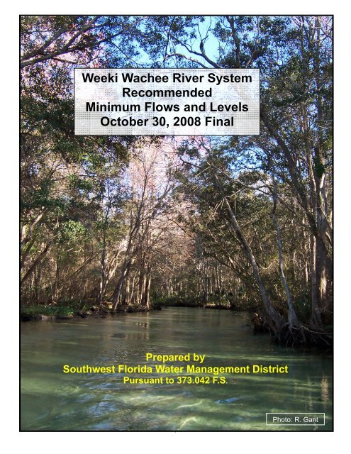
<strong>Weeki</strong> <strong>Wachee</strong> <strong>River</strong> <strong>System</strong><br />
<strong>Recommended</strong><br />
<strong>Minimum</strong> <strong>Flows</strong> <strong>and</strong> Levels<br />
October 30, 2008 Final<br />
Prepared by<br />
Southwest Florida Water Management District<br />
Pursuant to 373.042 F.S.<br />
i<br />
Photo: R. Gant
<strong>Weeki</strong> <strong>Wachee</strong> <strong>River</strong> <strong>Recommended</strong><br />
<strong>Minimum</strong> <strong>Flows</strong> <strong>and</strong> Levels<br />
October 30, 2008<br />
Ecologic Evaluation Section<br />
Resource Projects Department<br />
Southwest Florida Water Management District<br />
Brooksville, Florida 34604-6899<br />
Michael G. Heyl, MS<br />
Chief Environmental Scientist<br />
The Southwest Florida Water Management District (District) does<br />
not discriminate upon the basis of any individual's disability status.<br />
This non-discrimination policy involves every aspect of the<br />
District's functions, including one's access to, participation,<br />
employment, or treatment in its programs or activities. Anyone<br />
requiring accommodation as provided for in the American with<br />
Disabilities Act should contact (352) 796-7211 or 1-800-423-1476,<br />
extension 4215; TDD ONLY 1-800-231-6103; FAX (352) 754-<br />
6749.
Conversion Table<br />
Metric to U.S. Customary<br />
Multiply By To Obtain<br />
cubic meters per second (m 3 /s) 35.31 cubic feet per second (cfs)<br />
cubic meters per second (m 3 /s) 23 million gallons per day (mgd)<br />
millimeters (mm) 0.03937 inches (in)<br />
centimeter (cm) 0.3937 inches (in)<br />
meters (m) 3.281 feet (ft)<br />
kilometers (km) 0.6214 statute miles (mi)<br />
square meters (m 2 ) 10.76 square feet (ft 2 )<br />
square kilometers (km 2 ) 0.3861 square miles (mi 2 )<br />
hectares (ha) 2.471 acres<br />
liters (l) 0.2642 gallons<br />
cubic meters (m 3 ) 35.31 cubic feet (ft 3 )<br />
cubic meters (m 3 ) 0.0008110 acre-ft<br />
milligrams (mg) 0.00003527 ounces<br />
grams (g) 0.03527 ounces<br />
kilograms (kg) 2.205 pounds<br />
Celsius degrees ( o C) 1.8*( o C) + 32 Fahrenheit ( o F)<br />
US Customary to Metric<br />
inches (in) 25.40 millimeters (mm)<br />
inches (in) 2.54 centimeter (cm)<br />
feet (ft) 0.3048<br />
statute miles (mi) 1.609<br />
square feet (ft 2 ) 0.0929 square meters (m 2 )<br />
square miles (mi 2 ) 2.590 square kilometers (km 2 )<br />
acres 0.4047 hectares (ha)<br />
gallons (gal) 3.785 liters (l)<br />
cubic feet (ft 3 ) 0.02831 cubic meters (m 3 )<br />
acre-feet 1233.0 cubic meters (m 3 )<br />
Fahrenheit ( o F) 0.5556*( o F-32) Celsius degrees ( o C)<br />
US Customary to US Customary<br />
acre 43560 square feet (ft 2 )<br />
square miles (mi 2 ) 640 acres<br />
cubic feet per second (cfs) 0.646 million gallons per day (mgd)<br />
ii
Table of Contents<br />
CHAPTER 1 - PURPOSE & BACKGROUND OF MFL.......................................................................... 14<br />
1.1 OVERVIEW AND LEGISLATIVE DIRECTION .........................................................................................................14<br />
1.2 HISTORICAL PERSPECTIVE .................................................................................................................................15<br />
1.3 THE FLOW REGIME ............................................................................................................................................15<br />
1.4 ECOSYSTEM INTEGRITY AND SIGNIFICANT HARM .............................................................................................17<br />
1.4.1 Defining Significant Harm ........................................................................................................................17<br />
1.4.2 <strong>Minimum</strong> Evaluation Criteria ...................................................................................................................19<br />
1.5 SUMMARY OF THE SWFWMD APPROACH FOR DEVELOPING MINIMUM FLOWS ...............................................21<br />
1.5.1 Elements of <strong>Minimum</strong> <strong>Flows</strong>.....................................................................................................................21<br />
1.5.2 <strong>Flows</strong> <strong>and</strong> Levels.......................................................................................................................................22<br />
1.6 CONTENT OF REMAINING CHAPTERS .................................................................................................................24<br />
CHAPTER 2 - WATERSHED CHARACTERISTICS – PHYSICAL AND HYDROLOGY................... 26<br />
2.1 WATERSHED / SPRINGSHED ...............................................................................................................................26<br />
2.1.1 L<strong>and</strong> Use ...................................................................................................................................................28<br />
2.1.2 Hydrogeologic Setting...............................................................................................................................30<br />
2.1.3 History.......................................................................................................................................................31<br />
2.2 CLIMATE / METEOROLOGY ................................................................................................................................32<br />
2.3 FLOW AND HYDROGEOLOGY (ADAPTED FROM WOLFE 1990 AND KNOCHENMUS & YOBBI 2001) ....................34<br />
2.3.1 Discharge Estimates..................................................................................................................................35<br />
2.3.2 Baseline Period.........................................................................................................................................38<br />
2.4 HISTORICAL CHANGE IN DISCHARGE.................................................................................................................39<br />
2.5 CORRECTIONS FOR ANTHROPOGENIC IMPACTS..................................................................................................41<br />
2.5.1 Reference Approach..................................................................................................................................41<br />
2.5.2 Wavelet Analysis .......................................................................................................................................42<br />
2.5.3 Groundwater Model Estimate ...................................................................................................................44<br />
2.5.4 Flow Adjustment .......................................................................................................................................46<br />
2.6 SEASONAL BLOCKS............................................................................................................................................48<br />
2.7 MUD RIVER DISCHARGE....................................................................................................................................50<br />
CHAPTER 3 - ESTUARY CHARACTERISTICS .................................................................................... 51<br />
3.1 PHYSICAL ..........................................................................................................................................................51<br />
3.1.1 Linear........................................................................................................................................................51<br />
3.1.2 Area / Volume............................................................................................................................................52<br />
3.1.3 Segmentation.............................................................................................................................................54<br />
3.2 SEDIMENTS & BOTTOM HABITATS .....................................................................................................................54<br />
3.3 TIDAL WETLANDS & RIPARIAN HABITATS ........................................................................................................58<br />
CHAPTER 4 - TIDE, SALINITY & WATER QUALITY ........................................................................ 62<br />
4.1 TIDE...................................................................................................................................................................62<br />
4.2 SALINITY ...........................................................................................................................................................65<br />
4.2.1 Segment Salinity Estimation......................................................................................................................70<br />
4.2.2 Salinity Estimation – Bayport ...................................................................................................................72<br />
4.2.3 Isohaline Estimation..................................................................................................................................75<br />
4.2.4 Longitudinal Salinity Estimation...............................................................................................................77<br />
4.3 WATER QUALITY...............................................................................................................................................79<br />
CHAPTER 5 - BIOLOGICAL CHARACTERISTICS .............................................................................. 84<br />
5.1 BENTHOS ...........................................................................................................................................................84<br />
5.1.1 Descriptive ................................................................................................................................................84<br />
5.1.2 Relation to inflow ......................................................................................................................................84<br />
iii
5.2 FISH ...................................................................................................................................................................87<br />
5.2.1 Descriptive (Adapted from Matheson et al. 2005) ....................................................................................87<br />
5.2.2 Relation to inflow ......................................................................................................................................90<br />
5.3 MANATEE ..........................................................................................................................................................95<br />
5.3.1 Descriptive (Adapted from Laist <strong>and</strong> Reynolds (2005))............................................................................95<br />
5.3.2 Relation to inflow ......................................................................................................................................96<br />
5.4 MOLLUSC...........................................................................................................................................................99<br />
5.4.1 Descriptive ................................................................................................................................................99<br />
5.4.2 Relation to Inflow....................................................................................................................................102<br />
CHAPTER 6 - RESOURCES OF CONCERN & CRITERIA ................................................................. 105<br />
6.1 RESOURCE CRITERIA / GOALS - ESTUARINE ....................................................................................................105<br />
6.1.1 Fish & Invertebrates ...............................................................................................................................105<br />
6.1.2 Submerged Aquatic Vegetation ...............................................................................................................107<br />
6.1.3 Manatee...................................................................................................................................................107<br />
6.1.4 Benthos....................................................................................................................................................110<br />
6.1.5 Mollusc Criteria......................................................................................................................................110<br />
6.2 RESOURCE CRITERIA / GOALS – FRESHWATER ................................................................................................111<br />
CHAPTER 7 - TECHNICAL APPROACH............................................................................................. 113<br />
7.1 FISH / INVERTEBRATE TECHNICAL APPROACH.................................................................................................113<br />
7.2 MANATEE APPROACH......................................................................................................................................114<br />
7.3 BENTHOS TECHNICAL APPROACH....................................................................................................................119<br />
7.4 APPLICATION OF SALINITY HABITAT MODEL ..................................................................................................121<br />
7.5 MOLLUSC TECHNICAL APPROACH...................................................................................................................122<br />
7.6 APPROACH TO FRESHWATER MFL...................................................................................................................123<br />
CHAPTER 8 - CONCLUSIONS AND DISTRICT RECOMMENDATIONS FOR MFL...................... 125<br />
8.1 SUMMARY OF OUTCOMES................................................................................................................................125<br />
8.2 COMPLIANCE STANDARDS AND RECOMMENDED MINIMUM FLOWS FOR THE WEEKI WACHEE SYSTEM..........128<br />
CHAPTER 9 - LITERATURE CITED .................................................................................................... 129<br />
9.1 LITERATURE CITED - CHAPTER 1 .....................................................................................................................129<br />
9.2 LI TERATURE CITED - CHAPTER 2 ....................................................................................................................130<br />
9.3 LITERATURE CITED - CHAPTER 3 .....................................................................................................................132<br />
9.4 LITERATURE CITED - CHAPTER 4 .....................................................................................................................132<br />
9.5 LITERATURE CITED - CHAPTER 5 .....................................................................................................................133<br />
9.6 LITERATURE CITED - CHAPTER 6 .....................................................................................................................134<br />
9.7 LITERATURE CITED - CHAPTER 7 .....................................................................................................................135<br />
CHAPTER 10 - APPENDICES................................................................................................................ 136<br />
10.1 APPENDICES – CHAPTER 2 .............................................................................................................................136<br />
10.2 APPENDICES – CHAPTER 3 .............................................................................................................................160<br />
10.3 APPENDICES – CHAPTER 4 .............................................................................................................................162<br />
iv
LIST OF FIGURES<br />
Figure 2-1 Florida Springs Coast Sub-basins <strong>and</strong> <strong>Weeki</strong> <strong>Wachee</strong> Watershed ………14<br />
Figure 2-2 <strong>Weeki</strong> <strong>Wachee</strong> Watershed (yellow) <strong>and</strong> Springshed (green)………………..15<br />
Figure 2-3 Location of Springs <strong>and</strong> <strong>River</strong> Kilometers………………………………….....16<br />
Figure 2-4 1974 Aerial with Canal Development Periods…………………………………17<br />
Figure 2-5 1970s Aerial with 1999 Urban Areas Shaded Red…………………………...18<br />
Figure 2-6 Hurricane Tracks near Bayport Florida 1905-2005…………………………..20<br />
Figure 2-7 <strong>Weeki</strong> <strong>Wachee</strong> Flow/Water Level Regressions by Period………………......22<br />
Figure 2-8 Observed vs. Predicted <strong>Flows</strong> Using all Data 1966-2004……………………23<br />
Figure 2-9 Mean Monthly Discharge (cfs) 1966-2005…………………………………….24<br />
Figure 2-10 Distribution of Daily Discharge (cfs) <strong>and</strong> Discharge on Sample Days…….25<br />
Figure 2-11 Flow Comparison – Baseline Period (1984-2004) to Period of Record<br />
(1966-2005) Comparison of Sampling Days to Baseline Period…………………………25<br />
Figure 2-12 <strong>Weeki</strong> <strong>Wachee</strong> Annual Flow…………………………………………………...26<br />
Figure 2-13 <strong>Weeki</strong> <strong>Wachee</strong> Springshed Historical<br />
Pumpage………………………………………..27<br />
Figure 2-14 Original Data s. Wavelet Filtered Data………………………………………..29<br />
Figure 2-15 Wavelet Filtered Discharge vs. Predicted Discharge………………………..30<br />
Figure 2-16 Groundwater Model Spatial Domain…………………………………………..32<br />
Figure 2-17 Observed <strong>and</strong> Adjusted <strong>Flows</strong>…………………………………………………33<br />
Figure 2-18 Estimated Percent of Anthropogenic Flow Declines………………………...33<br />
Figure 2-19 Building Blocks for Development of <strong>Minimum</strong> <strong>Flows</strong> (<strong>Weeki</strong> <strong>Wachee</strong> 1984-<br />
2004)…………………………………………………………………………………………….35<br />
Figure 3-1 <strong>River</strong> Kilometer <strong>System</strong>…………………………………………………………..37<br />
v
Figure 3-2 Location of Bathymetric Survey Transects…………………………………….38<br />
Figure 3-3 Cumulative Upstream Volume <strong>and</strong> Area vs. <strong>River</strong> Kilometer………………..39<br />
Figure 3-4 <strong>Weeki</strong> <strong>Wachee</strong> <strong>and</strong> Mud <strong>River</strong> Segmentation Scheme………………………40<br />
Figure 3-5 Dominant SAV <strong>and</strong> Median Bottom Salinity 1984-2005……………………...42<br />
Figure 3-6 Sediment Characteristics – <strong>Weeki</strong> <strong>Wachee</strong> <strong>and</strong> Mud <strong>River</strong>s………………..44<br />
Figure 3-7 Shoreline/Buffer Vegetation – <strong>Weeki</strong> <strong>Wachee</strong> <strong>and</strong> Mud <strong>River</strong>s…………….46<br />
Figure 3-8 Aerial Photograph Illustrating Marsh Edge – <strong>Weeki</strong> <strong>Wachee</strong> <strong>and</strong> Mud<br />
<strong>River</strong>s………..…………………………………………………………………………………47<br />
Figure 4-1 <strong>Weeki</strong> <strong>Wachee</strong> Water Level at Mouth (green) <strong>and</strong> 3.7 km Upstream (red<br />
trace)………………..………………………………………………………………………….49<br />
Figure 4-2 Seasonal Variation in Mean Tide Level (NOAA 2001)………………………..50<br />
Figure 4-3 Observed <strong>and</strong> Predicted Deviations from MTL. Cedar Key, FL……………..50<br />
Figure 4-4 Bayport Tide, Observed <strong>and</strong> Predicted May 2001…………………………….51<br />
Figure 4-5 Median Bottom Salinity at Fixed Stations (2003-2005) <strong>and</strong> Segment<br />
Midpoints (1984-2005)………………………………………………………………………...52<br />
Figure 4-6 Number of Salinity Measurements (1984-2005) by <strong>River</strong> Kilometer………..53<br />
Figure 4-7 Salinity Range (1984-2005) by Segment Mid-Point…………………………..54<br />
Figure 4-8 Median Bottom Salinity (2003-2005) Red Trace………………………………56<br />
Figure 4-9 Isohaline Locations for Various Monitoring Programs (1984-2005)…………62<br />
Figure 4-10 Nitrate Concentration as Function of Salinity (1984-2005)…………………68<br />
Figure 4-11 Nitrate Concentration 1984-2005 for Salinity
Figure 5-3 Number of Aerial Manatee Surveys by Year <strong>and</strong> Refuge…………………….84<br />
Figure 5-4 Annual Average Number of Manatees – <strong>Weeki</strong> <strong>Wachee</strong> <strong>River</strong> <strong>and</strong> King's<br />
Bay………………………………………………………………………………………………84<br />
Figure 5-5(a) Molluscan Presence/Absence in <strong>Weeki</strong> <strong>Wachee</strong> <strong>and</strong> Mud <strong>River</strong>s……….86<br />
Figure 5-5(b) Molluscan Presence/Absence in <strong>Weeki</strong> <strong>Wachee</strong> <strong>and</strong> Mud <strong>River</strong>s……….87<br />
Figure 5-5 Polymesoda caroliniana Abundance as Function of Salinity in Tidal <strong>River</strong>s<br />
along West Coast of Florida………………………………………………………………….90<br />
Figure 6-1 Plankton Tow <strong>Flows</strong> Compared to Baseline…………………………………...92<br />
Figure 6-2 Example of Change in Volume > 20°C with Reduced <strong>Flows</strong> – <strong>Weeki</strong> <strong>Wachee</strong><br />
<strong>River</strong>…………………...………………………………………………………………….…...95<br />
Figure 6-3 Location of the Three PHABSIM Sites on the <strong>Weeki</strong> <strong>Wachee</strong> <strong>River</strong>………98<br />
Figure 7-1 <strong>Weeki</strong> <strong>Wachee</strong> Air Temperature vs. Bayport Water Temperature…………100<br />
Figure 7-2 Joint Probability of Occurrence – <strong>Weeki</strong> <strong>Wachee</strong> Thermal Regime<br />
Evaluations……………………………………………………………………………………102<br />
Figure 7-3 Maximum Day Manatee Usage – Blue Springs, Florida…………………….104<br />
Figure 7-4 Maximum Manatee Usage on Coldest Days – Blue Springs, Florida..........104<br />
Figure 7-5 Number of Manatees Supported by Baseline <strong>and</strong> Reduced <strong>Flows</strong> – <strong>Weeki</strong><br />
<strong>Wachee</strong>, Florida (3.8 foot minimum depth)………………………………………………..105<br />
Figure 7-6 Example Calculations for Benthic Diversity…………………………………..106<br />
Figure 7-7 Estimation of Flow Reduction Resulting in 15% Loss of Volume at 2 ppt...108<br />
Figure 7-8 Summary Results for the "wide" <strong>Weeki</strong> <strong>Wachee</strong> <strong>River</strong> PHABSIM Site……110<br />
Figure 7-9 Summary Results for the "s<strong>and</strong>bag" <strong>Weeki</strong> <strong>Wachee</strong> <strong>River</strong> PHABSIM<br />
Site……………………………………………………………………………………………..110<br />
Figure 8-1 Summary of <strong>Weeki</strong> <strong>Wachee</strong> MFL Results……………………………………113<br />
vii
LIST OF TABLES<br />
Table 1-1 Rule-of-Thumb Estimates for Number of Observations Needed……………....8<br />
Table 1-2 Number of Observations Considering Strength of Correlation.........................8<br />
Table 2-1 Watershed <strong>and</strong> Springshed L<strong>and</strong> Use…………………………………………..17<br />
Table 2-2 Hurricanes Passing within 65 Nautical Miles of Bayport Florida 1905 -<br />
2005……………………………………………………………………………………………..20<br />
Table 2-3 Summary of USGS Gauges Near <strong>Weeki</strong> <strong>Wachee</strong> <strong>River</strong>………………………22<br />
Table 2-4 Monthly Summary of <strong>Weeki</strong> <strong>Wachee</strong> Percentile Discharge (cfs) 1966-<br />
2005……….....................................................................................................................23<br />
Table 2-5 Comparison of Flow Adjustment Evaluations…………………………………..32<br />
Table 2-6 Median (cfs) Flow by Blocks 1984-2004………………...................................36<br />
Table 3-1 Bayport (28° 32.0' 82° 39.0') Tidal Benchmarks………………………………39<br />
Table 3-2 Results of <strong>Weeki</strong> <strong>Wachee</strong> Sediment Analysis<br />
………………………………………………………………..46<br />
Table 3-3 Percentage of <strong>Weeki</strong> <strong>Wachee</strong> Sites Where Species Occurred………………45<br />
Table 3-4 Wetl<strong>and</strong> Shoreline Vegetation Within 500 Meters……………………………..47<br />
Table 4-1 Comparison of Tide at Mouth <strong>and</strong> 3.7 Km Upstream………………………….48<br />
Table 4-2 Principal Tide Harmonics…………………………………………………………49<br />
Table 4-3 Median Salinity by <strong>River</strong> Segment……………………………………………….52<br />
Table 4-4 Salinity Predictions by Segment………………………………………………….57<br />
Table 4-5 Summary of Salinity Regression – By Segment, Depth, <strong>and</strong> Tide…………...58<br />
Table 4-6 Step-Wise Salinity Regression Bayport, Florida………………………………..61<br />
Table 4-7 Correlation (LOC) Summary – Isohaline Location.…………………………….63<br />
Table 4-8 Median Water Quality of <strong>Weeki</strong> <strong>Wachee</strong> <strong>and</strong> Mud <strong>River</strong>s (1985-2005)……..66<br />
viii
Table 5-1 Benthos Response to Salinity – <strong>Weeki</strong> <strong>Wachee</strong>, Mud, <strong>and</strong> Chassahowitzka<br />
<strong>River</strong>s……………………………………………………………………………………………70<br />
Table 5-2 Benthos Response to Normalized (Z-score) Physical – Chemical<br />
Parameters……………………………………………………………………………………..71<br />
Table 5-3 Fish/Invertebrate Sampling Zones…………………….....................................73<br />
Table 5-4 Estuarine Usage by Taxa Captured in <strong>Weeki</strong> <strong>Wachee</strong> <strong>River</strong>…………………75<br />
Table 5-5 Summary of Data Transformers – Plankton <strong>and</strong> Fish…………………………76<br />
Table 5-6 Location Response (kmµ) – Plankton Net Capture……………………………77<br />
Table 5-7 Location Response (kmµ) – Seine <strong>and</strong> Trawl Capture………………………..78<br />
Table 5-8 Abundance Response to Inflow, Plankton Net Capture……………………….79<br />
Table 5-9 Abundance Response to Inflow – Seine <strong>and</strong> Trawl Capture………………….80<br />
Table 5-10 Average Number of Surveys <strong>and</strong> Manatee Counts – Florida West Coast<br />
1996-2005………………………………………………………………………………………83<br />
Table 5-11 Rank Order of Mollusc Abundance in the Mud <strong>and</strong> <strong>Weeki</strong> <strong>Wachee</strong> <strong>River</strong><br />
(Estevez, 2005)………………………………………………………………………………...88<br />
Table 5-12 Rank Mollusc Abundance – Florida West Coast Tidal <strong>River</strong>s……...............89<br />
Table 5-13 Response Parameters for Dominant Native Mollusc in <strong>Weeki</strong> <strong>Wachee</strong> <strong>and</strong><br />
Mud <strong>River</strong>s……………………………………………………………………………………..90<br />
Table 6-1 Baseline <strong>Flows</strong> for Evaluation of Fish/Invertebrate Losses…………………..92<br />
Table 6-2 Dominant SAV – Location of Maximum Density <strong>and</strong> Expected<br />
Salinities……………….……………………………………………………………………….93<br />
Table 6-3 Manatee Thermal Criteria…..…………………………………………………….94<br />
Table 6-4 Benthic Community Criteria……………………………………………………..96<br />
Table 7-1 Response of Pinfish Abundance to Reduced Flow in the <strong>Weeki</strong> <strong>Wachee</strong><br />
<strong>River</strong>…………………………………………………………………………………………...99<br />
Table 7-2 Thermal Refuge Reductions Due to Reduced <strong>Flows</strong>………………………...103<br />
ix
Table 8-1 Summary of <strong>Weeki</strong> <strong>Wachee</strong> MFL Results…………………………………….112<br />
Table 8-2 Long-Term <strong>Minimum</strong> <strong>Flows</strong> Corresponding to <strong>Recommended</strong><br />
MFL………………………………………………………………………………………….114<br />
x
Preface<br />
This report was prepared by the Southwest Florida Water Management District pursuant<br />
to Florida Statute 473.042. A draft was made available to the public on April 14, 2008<br />
<strong>and</strong> submitted to an independent peer review panel consisting of Dr. Joseph Boyer<br />
(Fla. International University), Dr. 'Billy' Johnson (Computational Hydraulics Inc), Mr.<br />
Gary Powell (Aquatic Science Associates) <strong>and</strong> Dr. Sam Upchurch (SDII Global). Among<br />
other things, the panel was directed to determine whether the methods used for<br />
establishing the minimum flow are scientifically reasonable, if the assumptions <strong>and</strong><br />
procedures are reasonable <strong>and</strong> consistent with the best information available <strong>and</strong> if the<br />
District's conclusions are supported by the data. The panel submitted their report on<br />
July 31, 2008, which is appended to this along with the District's response. In addition,<br />
the US Fish <strong>and</strong> Wildlife Service <strong>and</strong> the Florida Fish <strong>and</strong> Wildlife Conservation<br />
Commission reviewed the report <strong>and</strong> submitted comments that are also appended. This<br />
final report reflects the comments <strong>and</strong> suggestions received.<br />
Acknowledgements<br />
I would like to thank my colleagues for the many useful suggestions <strong>and</strong> discussions<br />
pertinent to completion of this project. In particular I would like to acknowledge Marty<br />
Kelly, Rich Schultz, Ron Basso for their assistance in deriving corrections to the<br />
historical flow record. I would also like to thank Sid Flannery, XinJian Chen <strong>and</strong> Tony<br />
Janicki <strong>and</strong> his staff. I would like to offer a special thanks to Michelle Dachsteiner for<br />
her dedication to the field work <strong>and</strong> data management as well as Barbara Matrone for<br />
her assistance in document production.<br />
Finally I would like to thank the many District contractors that contributed to this report.<br />
Ernst Peebles (<strong>and</strong> his staff at USF) <strong>and</strong> Tim MacDonald <strong>and</strong> his colleagues at Florida<br />
Fish <strong>and</strong> Wildlife Conservation Commission collected <strong>and</strong> analyzed the fish <strong>and</strong><br />
invertebrate data. Ernie Estevez conducted field surveys of mollusk use of the <strong>Weeki</strong><br />
<strong>Wachee</strong>, <strong>and</strong> along with Jay Leverone conducted a survey of the macrophyte<br />
community. Paul Montagna provided insightful analysis of mollusc data. The staff at<br />
Janicki Environmental conducted a survey <strong>and</strong> analysis of the benthic community <strong>and</strong><br />
along with staff from Applied Technology <strong>and</strong> Management, provided numeric modeling<br />
results for the thermal refuge analysis. While several of these projects were regional in<br />
nature, the cost of outside support is approximately $300,000 which was provided by<br />
Coastal <strong>River</strong>s Basin Board <strong>and</strong> the Governing Board.<br />
xi
Executive Summary<br />
<strong>Minimum</strong> <strong>Flows</strong> <strong>and</strong> Levels – <strong>Weeki</strong> <strong>Wachee</strong> <strong>River</strong><br />
The <strong>Weeki</strong> <strong>Wachee</strong> <strong>River</strong> originates from <strong>Weeki</strong> <strong>Wachee</strong> Spring which discharges at a<br />
relatively constant rate from the Floridan aquifer. The river receives a small amount of<br />
surface runoff from its 38 mi 2 watershed, but the overwhelming majority of flow arises<br />
from the 260 + mi 2 springshed. The river flows 7.4 miles (12 km) from the headspring to<br />
the Gulf of Mexico at Bayport in Hern<strong>and</strong>o County, Florida. Daily discharge is estimated<br />
by the United States Geological Survey (USGS) as a function of water level in a nearby<br />
well completed in the Floridan. By comparison to other rivers on the west coast of<br />
Florida, the estuarine portion is very compressed with rapidly decreasing salinities over<br />
a short stretch of the river. Typically freshwater (< 0.5 ppt) is encountered 1.6 miles (2.6<br />
km) upstream from the confluence with the Gulf. Near Gulf salinity tends to be relatively<br />
low along the shallow, but open coastal area west of the <strong>Weeki</strong> <strong>Wachee</strong> <strong>River</strong>. Average<br />
(1985-2005) bottom salinity at the mouth ( + 0.5 km) is approximately thirty percent (11<br />
ppt) of full seawater strength.<br />
The salinity structure within the <strong>Weeki</strong> <strong>Wachee</strong> <strong>River</strong> is complicated by discharge from<br />
the Mud <strong>River</strong> which joins the <strong>Weeki</strong> <strong>Wachee</strong> <strong>River</strong> 0.9 miles (1.4 km) from the Gulf.<br />
Flow in the Mud <strong>River</strong> originates from Mud Spring <strong>and</strong> Salt Spring located<br />
approximately 1.6 miles (2.5 km) up the Mud <strong>River</strong>. This river is tidally influenced to the<br />
headwaters. Discharge from these two sources has not been routinely monitored,<br />
although sporadic measurements have been made <strong>and</strong> the discharge ranges from –51<br />
to +78 cfs. The discharge is saline (~ 12 ppt) <strong>and</strong> discharge is sufficient to cause a<br />
measurable increase in salinity (reverse estuary) at the confluence of the Mud <strong>River</strong><br />
with the <strong>Weeki</strong> <strong>Wachee</strong> <strong>River</strong>.<br />
Discharge from the <strong>Weeki</strong> <strong>Wachee</strong> Spring has averaged approximately 174 cfs for the<br />
period of record (1935-2004) <strong>and</strong> 162 cfs for the baseline period (1984-2004) chosen<br />
for establishing the MFL. Daily estimates are available from 1974 to present, <strong>and</strong><br />
annual average flows peaked in 1960 at 253 cfs. Anthropogenic impacts, primarily<br />
ground water pumpage from the springshed, have resulted in an estimated 17 cfs<br />
decline since 1961, or the equivalent of a eight percent reduction in flow during 2004.<br />
A broad spectrum of ecological resources were identified <strong>and</strong> evaluated for sensitivity to<br />
reduced flows using both numeric models <strong>and</strong> empirical regressions. Resources<br />
considered included salinity habitat, fish <strong>and</strong> invertebrates, benthic communities,<br />
mollusc, submerged aquatic vegetation (SAV) <strong>and</strong> thermal refuge for manatees in the<br />
estuary. Criteria evaluated for the freshwater reaches included twelve life-stage habitat<br />
requirements for fish <strong>and</strong> an evaluation of benthic community diversity. Break-points in<br />
ecological response were not observed, <strong>and</strong> a fifteen percent loss of resource was<br />
adopted as representing significant harm.<br />
After evaluation, the results for several resources were excluded from the determination<br />
of the MFL. While the loss of thermal refuge for manatees exceeded the a priori<br />
xii
criterion at a five percentage flow reduction, the amount of refuge remaining at even a<br />
twenty five percent flow reduction was sufficient in volume <strong>and</strong> area to support 40 (low<br />
flow scenario) to 120 times (high flow scenario) the number of animals that currently use<br />
the <strong>Weeki</strong> <strong>Wachee</strong> <strong>River</strong> <strong>and</strong> was sufficient to house the entire manatee population<br />
found north of Tampa Bay. Based on aerial surveys, the average number of manatees<br />
using the <strong>Weeki</strong> <strong>Wachee</strong>/Mud <strong>River</strong> system is 10 animals. The northern Tampa Bay<br />
population is estimated at 400 animals. Thus, the a priori fifteen percent reduction was<br />
deemed inappropriately conservative for application in the <strong>Weeki</strong> <strong>Wachee</strong> <strong>River</strong>.<br />
The response (abundance) of fish <strong>and</strong> invertebrates to reductions in flow was not<br />
incorporated into the recommended MFL. Flow during the period of time when fish /<br />
invertebrate abundance was measured was abnormally high which severely limits the<br />
range over which estimates can be made. Applying the abundance to flow response<br />
developed with the higher flows resulted in a prediction that certain fish common to the<br />
<strong>Weeki</strong> <strong>Wachee</strong> would be essentially absent during median flow conditions that existed<br />
throughout the baseline period.<br />
Finally, the SAV results were inconsistent. The approach utilized was to relate the<br />
location of maximum density for each native species to the estimated long-term bottom<br />
salinity at that location. However, when the median salinity at the location of various<br />
taxa in the <strong>Weeki</strong> <strong>Wachee</strong> <strong>River</strong> were compared with the median salinity at the location<br />
of the same species in the Mud <strong>River</strong>, inconsistencies became apparent that suggest<br />
that factors other than salinity may be more important in shaping the SAV distributions.<br />
Ordinarily, the MFL recommendation is based on the resource most sensitive to<br />
reduced flow. In the case of the <strong>Weeki</strong> <strong>Wachee</strong>, the loss of 15 ppt habitat was most<br />
sensitive, but this salinity was predicted to occur below the Mud <strong>River</strong> during the low<br />
flows evaluated <strong>and</strong> in the Gulf of Mexico beyond the mouth of the river during high<br />
flow. The latter necessitated extrapolating results from within the defined river channel.<br />
The high salinity of the Mud <strong>River</strong> <strong>and</strong> the fact that Mud <strong>River</strong> discharge is not well<br />
characterized led to a decision to not base the MFL on these higher salinity results, but<br />
rather to include those results as part of an average of all the remaining resource<br />
responses.<br />
A total of sixteen responses were averaged for both low flow conditions <strong>and</strong> high flow<br />
conditions. In each case the reduction in flow resulting in a fifteen percent loss of<br />
resource or habitat was determined <strong>and</strong> included. The mean reduction in flow for the<br />
wet season evaluations was 10.7 percent while the mean reduction for the dry season<br />
was 10.1 percent. In consideration of the results, the proposed MFL for the <strong>Weeki</strong><br />
<strong>Wachee</strong> spring <strong>and</strong> river s a ten percent reduction in flows that have been corrected for<br />
pumpage impacts. There are no consistent, long-term flow measurements for Mud<br />
Springs, Salt Springs, Mud <strong>River</strong>, Jenkins Springs or Twin Dees Spring. Thus, in the<br />
absence of sufficient data to evaluate these individually, the assumed MFL for these<br />
waterbodies is also ten percent reduction in baseline flows.<br />
xiii
CHAPTER 1 - PURPOSE & BACKGROUND OF MFL<br />
1.1 Overview <strong>and</strong> Legislative Direction<br />
The Southwest Florida Water Management District (District or SWFWMD), by virtue of<br />
its responsibility to permit the consumptive use of water <strong>and</strong> a legislative m<strong>and</strong>ate to<br />
protect water resources from “significant harm”, has been directed to establish minimum<br />
flows <strong>and</strong> levels (MFLs) for streams <strong>and</strong> rivers within its boundaries (Section 373.042,<br />
Florida Statutes). As currently defined by statute, “the minimum flow for a given<br />
watercourse shall be the limit at which further withdrawals would be significantly<br />
harmful to the water resources or ecology of the area.” Mere development or<br />
adoption of a minimum flow, of course, does not protect a water body from significant<br />
harm; however, protection, recovery or regulatory compliance can be gauged once a<br />
st<strong>and</strong>ard has been established. The District's purpose in establishing MFLs is to create<br />
a yardstick against which permitting <strong>and</strong>/or planning decisions regarding water<br />
withdrawals, either surface or groundwater, can be made. Should an amount of<br />
withdrawal requested cause “significant harm” then a permit cannot be issued. If, when<br />
developing MFLs, it is determined that a system is already significantly harmed as a<br />
result of existing withdrawals, then a recovery plan is developed <strong>and</strong> implemented.<br />
According to state law, minimum flows <strong>and</strong> levels are to be established based upon the<br />
best information available (Section 373.042, F.S), <strong>and</strong> shall be developed with<br />
consideration of “...changes <strong>and</strong> structural alterations to watersheds, surface waters<br />
<strong>and</strong> aquifers <strong>and</strong> the effects such changes or alterations have had, <strong>and</strong> the constraints<br />
such changes or alterations have placed, on the hydrology of the affected watershed,<br />
surface water, or aquifer...” (Section 373.0421, F.S.). Changes, alterations <strong>and</strong><br />
constraints associated with water withdrawals are not to be considered when<br />
developing minimum flows <strong>and</strong> levels. However, according to the State Water<br />
Resources Implementation Rule (Chapter 62-40.473, Florida Administrative Code),<br />
“consideration shall be given to the protection of water resources, natural seasonal<br />
fluctuations in water flows or levels, <strong>and</strong> environmental values associated with coastal,<br />
estuarine, aquatic <strong>and</strong> wetl<strong>and</strong>s ecology, including:<br />
1) Recreation in <strong>and</strong> on the water;<br />
2) Fish <strong>and</strong> wildlife habitats <strong>and</strong> the passage of fish;<br />
3) Estuarine resources;<br />
4) Transfer of detrital material;<br />
5) Maintenance of freshwater storage <strong>and</strong> supply;<br />
6) Aesthetic <strong>and</strong> scenic attributes;<br />
7) Filtration <strong>and</strong> absorption of nutrients <strong>and</strong> other pollutants;<br />
8) Sediment loads;<br />
9) Water quality; <strong>and</strong><br />
________________________________________________________________________________________________________<br />
Proposed <strong>Minimum</strong> <strong>Flows</strong> <strong>and</strong> Levels for <strong>Weeki</strong> <strong>Wachee</strong> <strong>River</strong><br />
Purpose <strong>and</strong> Background Page 1 of 164
10) Navigation".<br />
Because minimum flows are used for long-range planning <strong>and</strong> since the setting of<br />
minimum flows can potentially impact (restrict) the use <strong>and</strong> allocation of water,<br />
establishment of minimum flows will not go unnoticed or unchallenged. The science<br />
upon which a minimum flow is based, the assumptions made, <strong>and</strong> the policy used must<br />
therefore be clearly defined as each minimum flow is developed.<br />
1.2 Historical Perspective<br />
For freshwater streams <strong>and</strong> rivers, the development of instream flow legislation can be<br />
traced to the work of fisheries biologists. Major advances in instream flow methods<br />
have been rather recent, dating back not much more than 35 to 40 years. A survey<br />
completed in 1986 (Reiser et al. 1989) indicated that at that time only 15 states had<br />
legislation explicitly recognizing that fish <strong>and</strong> other aquatic resources required a certain<br />
level of instream flow for their protection. Nine of the 15 states were western states<br />
“where the concept for <strong>and</strong> impetus behind the preservation of instream flows for fish<br />
<strong>and</strong> wildlife had its origins” (Reiser et al. 1989). Stalnaker et. al (1995) have<br />
summarized the minimum flows approach as one of st<strong>and</strong>ards development, stating<br />
that, “[f]ollowing the large reservoir <strong>and</strong> water development era of the mid-twentieth<br />
century in North America, resource agencies became concerned over the loss of many<br />
miles of riverine fish <strong>and</strong> wildlife resources in the arid western United States.<br />
Consequently, several western states began issuing rules for protecting existing stream<br />
resources from future depletions caused by accelerated water development. Many<br />
assessment methods appeared during the 1960's <strong>and</strong> early 1970's. These techniques<br />
were based on hydrologic analysis of the water supply <strong>and</strong> hydraulic considerations of<br />
critical stream channel segments, coupled with empirical observations of habitat quality<br />
<strong>and</strong> an underst<strong>and</strong>ing of riverine fish ecology . . . Application of these methods usually<br />
resulted in a single threshold or ‘minimum’ flow value for a specified stream reach.”<br />
1.3 The Flow Regime<br />
The idea that a single minimum flow is not satisfactory for maintaining a river ecosystem<br />
was most emphatically stated by Stalnaker (1990) who declared that “minimum flow is a<br />
myth”. The purpose of his paper was to argue that “multiple flow regimes are needed to<br />
maintain biotic <strong>and</strong> abiotic resources within a river ecosystem” (Hill et al. 1991). The<br />
logic is that “maintenance of stream ecosystems rests on streamflow management<br />
practices that protect physical processes which, in turn, influence biological systems.”<br />
Hill et al. (1991) identified four types of flows that should be considered when examining<br />
river flow requirements, including:<br />
________________________________________________________________________________________________________<br />
Proposed <strong>Minimum</strong> <strong>Flows</strong> <strong>and</strong> Levels for <strong>Weeki</strong> <strong>Wachee</strong> <strong>River</strong><br />
Purpose <strong>and</strong> Background Page 2 of 164
1) flood flows that determine the boundaries of <strong>and</strong> shape floodplain <strong>and</strong> valley<br />
features;<br />
2) overbank flows that maintain riparian habitats;<br />
3) in-channel flows that keep immediate streambanks <strong>and</strong> channels functioning;<br />
<strong>and</strong><br />
4) in-stream flows that meet critical fish requirements.<br />
As emphasized by Hill et al. (1991), minimum flows methodologies should involve more<br />
than a consideration of immediate fish needs or the absolute minimum required to<br />
sustain a particular species or population of animals, <strong>and</strong> should take into consideration<br />
“how streamflows affect channels, transport sediments, <strong>and</strong> influence vegetation.”<br />
Although, not always appreciated, it should also be noted “that the full range of natural<br />
intra- <strong>and</strong> inter-annual variation of hydrologic regimes is necessary to [fully] sustain the<br />
native biodiversity” (Richter et al. 1996). Successful completion of the life-cycle of many<br />
aquatic species is dependant upon a range of flows, <strong>and</strong> alterations to the flow regime<br />
may negatively impact these organisms as a result of changes in physical, chemical <strong>and</strong><br />
biological factors associated with particular flow conditions.<br />
Recently, South African researchers, as cited by Postel <strong>and</strong> Richter (2003), listed eight<br />
general principles for managing river flows:<br />
1) "A modified flow regime should mimic the natural one, so that the natural<br />
timing of different kinds of flows is preserved.<br />
2) A river's natural perenniality or nonperenniality should be retained.<br />
3) Most water should be harvested from a river during wet months; little should<br />
be taken during the dry months.<br />
4) The seasonal pattern of higher baseflows in wet season should be retained.<br />
5) Floods should be present during the natural wet season.<br />
6) The duration of floods could be shortened, but within limits.<br />
7) It is better to retain certain floods at full magnitude <strong>and</strong> to eliminate others<br />
entirely than to preserve all or most floods at diminished levels.<br />
8) The first flood (or one of the first) of the wet season should be fully retained."<br />
Common to this list <strong>and</strong> the flow requirements identified by Hill et al (1991) is the<br />
recognition that in-stream flows <strong>and</strong> out of bank flows are important <strong>and</strong> that seasonal<br />
variability of flows should be maintained. Based on these concepts, the preconception<br />
that minimum flows (<strong>and</strong> levels) are a single value or the absolute minimum required to<br />
maintain ecologic health in most systems has been ab<strong>and</strong>oned in recognition of the<br />
important ecologic <strong>and</strong> hydrologic functions of streams <strong>and</strong> rivers that are maintained by<br />
different ranges of flow. And while the term “minimum flows” is still used, the concept<br />
has evolved to one that recognizes the need to maintain a “minimum flow regime”. In<br />
Florida, for example, the St. Johns <strong>River</strong> Water Management District (typically develops<br />
multiple flows requirements when establishing minimum flows <strong>and</strong> levels (Chapter 40-<br />
C8, F.A.C) <strong>and</strong> for the Wekiva <strong>River</strong> noted that, “[s]etting multiple minimum levels <strong>and</strong><br />
flows, rather than a single minimum level <strong>and</strong> flow, recognizes that lotic [running water]<br />
________________________________________________________________________________________________________<br />
Proposed <strong>Minimum</strong> <strong>Flows</strong> <strong>and</strong> Levels for <strong>Weeki</strong> <strong>Wachee</strong> <strong>River</strong><br />
Purpose <strong>and</strong> Background Page 3 of 164
systems are inherently dynamic” (Hupalo et al. 1994). An alternate approach which<br />
also maintains a flow regime is to develop MFLs using a 'percentage of flow' as<br />
discussed in Flannery et al. (2002) <strong>and</strong> has been incorporated into several SWFWMD<br />
surface water use permits.<br />
1.4 Ecosystem Integrity <strong>and</strong> Significant Harm<br />
“A goal of ecosystem management is to sustain ecosystem integrity by protecting native<br />
biodiversity <strong>and</strong> the ecological (<strong>and</strong> evolutionary) processes that create <strong>and</strong> maintain<br />
that diversity. Faced with the complexity inherent in natural systems, achieving that<br />
goal will require that resource managers explicitly describe desired ecosystem structure,<br />
function, <strong>and</strong> variability; characterize differences between current <strong>and</strong> desired<br />
conditions; define ecologically meaningful <strong>and</strong> measurable indicators that can mark<br />
progress toward ecosystem management <strong>and</strong> restoration goals; <strong>and</strong> incorporate<br />
adaptive strategies into resource management plans” (Richter et al. 1996). Although it<br />
is clear that multiple flows are needed to maintain the ecological systems that<br />
encompass streams, riparian zones <strong>and</strong> valleys, much of the fundamental research<br />
needed to quantify the ecological links between the instream <strong>and</strong> out of bank resources,<br />
because of expense <strong>and</strong> complexity, remains to be done. This research is needed to<br />
develop more refined methodologies, <strong>and</strong> will require a multi-disciplinary approach<br />
involving hydrologists, geomorphologists, aquatic <strong>and</strong> terrestrial biologists, <strong>and</strong><br />
botanists (Hill et al. 1991).<br />
To justify adoption of a minimum flow for purposes of maintaining ecologic integrity, it is<br />
necessary to demonstrate with site-specific information the ecological effects associated<br />
with flow alterations <strong>and</strong> to also identify thresholds for determining whether these effects<br />
constitute significant harm. As described in Florida’s legislative requirement to<br />
develop minimum flows, the minimum flow is to prevent “significant harm” to the state’s<br />
rivers <strong>and</strong> streams. Not only must “significant harm” be defined so that it can be<br />
measured, it is also implicit that some deviation from the purely natural or existing longterm<br />
hydrologic regime may occur before significant harm occurs. The goal of a<br />
minimum flow would, therefore, not be to preserve a hydrologic regime without<br />
modification, but rather to establish the threshold(s) at which modifications to the regime<br />
begin to affect the aquatic resource <strong>and</strong> at what level significant harm occurs. If recent<br />
changes have already “significantly harmed” the resource, or are expected to do so in<br />
the next twenty years, it will be necessary to develop a recovery or prevention plan.<br />
1.4.1 Defining Significant Harm<br />
The goal of an MFL determination is to protect the resource from significant harm due to<br />
withdrawals <strong>and</strong> was broadly defined in the enacting legislation as "the limit at which<br />
further withdrawals would be significantly harmful to the water resources or ecology of<br />
________________________________________________________________________________________________________<br />
Proposed <strong>Minimum</strong> <strong>Flows</strong> <strong>and</strong> Levels for <strong>Weeki</strong> <strong>Wachee</strong> <strong>River</strong><br />
Purpose <strong>and</strong> Background Page 4 of 164
the area." What constitutes "significant harm" was not defined. The District has<br />
identified loss of flows associated with fish passage <strong>and</strong> maximization of stream bottom<br />
habitat with the least amount of flow as significantly harmful to river ecosystems. Also,<br />
based upon consideration of a recommendation of the peer review panel for the upper<br />
Peace <strong>River</strong> MFLs (Gore et al. 2002), significant harm in many cases can be defined as<br />
quantifiable reductions in habitat.<br />
Ideally there will be a clear 'break point' that identifies significant harm. Unfortunately,<br />
more often in nature there is simply a monotonic continuum with a changing rate of<br />
response, but one that does not provide an easily identifiable break-point. Little<br />
guidance is found in the literature, <strong>and</strong> the definition of 'significant harm' often becomes<br />
a policy decision rather than a technical decision.<br />
In their peer review report o the Upper Peace <strong>River</strong>, Gore et al. (2002) stated, [i]n<br />
general, instream flow analysts consider a loss of more than 15% habitat, as compared<br />
to undisturbed or current conditions, to be a significant impact on that population or<br />
assemblage. This recommendation was made in consideration of employing the<br />
Physical Habitat Simulation Model (PHABSIM) for analyzing flow, water depth <strong>and</strong><br />
substrate preferences that define aquatic species habitats. With some exceptions<br />
(e.g., loss of fish passage or wetted perimeter inflection point), there are few "bright<br />
lines" which can be relied upon to judge when "significant harm" occurs. Rather loss of<br />
habitat in many cases occurs incrementally as flows decline, often without a clear<br />
inflection point or threshold.<br />
Based on Gore et al. (2002) comments regarding significant impacts of habitat loss, we<br />
recommend use of a 15% change in habitat availability as a measure of significant harm<br />
for the purpose of MFLs development. Although we recommend a 15% change in<br />
habitat availability as a measure of unacceptable loss, it is important to note that<br />
percentage changes employed for other instream flow determinations have ranged from<br />
10% to 33%. For example, Dunbar et al. (1998) in reference to the use of PHABSIM<br />
noted, "an alternative approach is to select the flow giving 80% habitat exceedance<br />
percentile," which is equivalent to a 20% decrease. Jowett (1993) used a guideline of<br />
one-third loss (i.e., retention of two-thirds) of existing habitat at naturally occurring low<br />
flows, but acknowledged that, "[n]o methodology exists for the selection of a percentage<br />
loss of "natural" habitat which would be considered acceptable." Powell et al. (2002)<br />
developed a procedure using optimization modeling techniques which the state of<br />
Texas applied to Galveston Bay <strong>and</strong> the Trinity-San Jacinto estuaries. The procedure is<br />
based on a harvest constraint that no individual species would be less than eighty<br />
percent of historical average. An additional constraint was imposed that the optimal<br />
solution falls between the 10 th <strong>and</strong> 50 th percentile of historical flows 1 .<br />
1 http://www.tpwd.state.tx.us/texaswater/coastal/freashwater/matagorda/matagorda.phtml<br />
________________________________________________________________________________________________________<br />
Proposed <strong>Minimum</strong> <strong>Flows</strong> <strong>and</strong> Levels for <strong>Weeki</strong> <strong>Wachee</strong> <strong>River</strong><br />
Purpose <strong>and</strong> Background Page 5 of 164
1.4.2 <strong>Minimum</strong> Evaluation Criteria<br />
Relating inherently variable biological responses to MFL objectives will ultimately<br />
require setting criteria for taking management action based on the strength of the<br />
biological response to flows or levels. The science of establishing MFLs is evolving <strong>and</strong><br />
many researchers have turned to regression statistics to determine the statistical<br />
strength between biological responses <strong>and</strong> inflows. The most common measure of the<br />
strength is the correlation coefficient (r) which ranges from +1.0 to 0.0 for a response<br />
that increases with increasing flow (conversely r can range from -1.0 to 0 for an inverted<br />
response). The coefficient of determination (r 2 ) is convenient, because it reflects the<br />
fraction of response that is attributable to changes in flow. However, it must be<br />
recognized that a statistically significant relationship may still be of limited value in the<br />
management of the resource. Taking an example from fish monitoring, it is possible to<br />
have statistically significant relationships that relate the number of animals to flow, but<br />
often the coefficient of determination is very low (e.g. 0.1). The interpretation is that<br />
while there is a significant relationship between the number of organisms <strong>and</strong> flow, flow<br />
only accounts for 10% of the change in numbers. The remaining 90% of variation in<br />
numbers is due to residual variation in flow <strong>and</strong> to factor(s) other than flow.<br />
The management question then becomes 'How much weight do we place on this<br />
relationship? Should we set flow limits when the majority of response is due to<br />
something other than flow? '. Comrey <strong>and</strong> Lee (1992) attempted to qualify correlation<br />
coefficient levels 2 according to the following schema:<br />
Coefficient of Descriptor<br />
Determination(r 2 )<br />
0.50 Excellent<br />
0.40 Very Good<br />
0.30 Good<br />
0.20 Fair<br />
0.10 Poor<br />
A similar problem facing the decision-makers is 'how much data do we need?'. Taken<br />
in the context of establishing statistical relationships between flow <strong>and</strong> ecological<br />
resources the analogous question is "How many data points should I have to develop<br />
my regression equation?' Research has shown that as the strength of the relationship<br />
diminishes, the number of observations required increases (so called 'effect size').<br />
Brooks <strong>and</strong> Barcikowski (1994) summarized several 'rule-of-thumb' approaches (Table<br />
1-1) taken from the literature <strong>and</strong> contrasted those results (Table 1-2) derived from their<br />
own Monte Carlo simulations <strong>and</strong> those promoted by Park <strong>and</strong> Dudycha (1974).<br />
2 Described in the context of evaluating orthogonal factor loadings resulting from factor analysis<br />
________________________________________________________________________________________________________<br />
Proposed <strong>Minimum</strong> <strong>Flows</strong> <strong>and</strong> Levels for <strong>Weeki</strong> <strong>Wachee</strong> <strong>River</strong><br />
Purpose <strong>and</strong> Background Page 6 of 164
Table 1-1<br />
Rule-of-Thumb Estimates for Number of Observations Needed<br />
Number of<br />
Observations/<br />
parameter<br />
Citation<br />
Miller & Kenuc, 1973. p 162<br />
10 * p Neter, Wasserman & Kutner. 1990. p 467<br />
> 15 * p Stevens, 1992. p 125<br />
Tabachnick & Fidell. 1989 p128 (N>100 preferred)<br />
Halinski & Feldt 1970 p157 (for identifying predictors)<br />
20 * p<br />
30 * p Pedhazur & Schmelkin. 1990. p 447<br />
> 40 * p Nunnally 1978. Tabachnick & Fidell 1989. p 129 (for step-wise)<br />
50 + p Harris, 1985. p 64<br />
10p + 50 Thorndike, 1978. p 184<br />
> 100 Kerlinger & Pedhazur. 1973. p 442 (preferably > 200)<br />
Adapted from Brooks, G.P. <strong>and</strong> R.S. Barcikowski 1994. A New Sample Size Formula for<br />
Regression. Presented at the Annual Meeting of the American Educational Research Association.<br />
New Orleans, LA April 1994.<br />
Table 1-2<br />
Number of Observations Considering Strength of Correlation<br />
Brooks & Barcikowski Park & Dudycha<br />
Number of<br />
Independent<br />
Variables<br />
r 2 ><br />
0.50<br />
r 2 ><br />
0.25<br />
r 2 ><br />
0.10<br />
r 2 ><br />
0.50<br />
r 2 ><br />
0.25<br />
r 2 ><br />
0.10<br />
2 42 62 122 31 45 85<br />
3 63 93 183 50 71 133<br />
4 84 124 244 66 93 173<br />
While, it would be desirable to have the number of observations suggested by Brooks<br />
<strong>and</strong> Barcikowski, most of the environmental observations used to develop an MFL<br />
cannot be designed <strong>and</strong> tested in laboratory conditions. The practical reality is that<br />
achieving the recommended number of observations rarely happens. Furthermore, the<br />
infrequent event is often the one of most interest. For example, it is important to know<br />
the maximum upstream penetration of saline water during abnormally dry conditions. As<br />
a second example, the fishery biologist has no real control over how many fish of a<br />
particular taxa will be caught in a seine.<br />
Thus, it often becomes necessary to try <strong>and</strong> develop relationships between flow <strong>and</strong><br />
some response with considerably fewer observations than recommended or desirable.<br />
While the legislature has indicated that an MFL should be based on the 'best<br />
________________________________________________________________________________________________________<br />
Proposed <strong>Minimum</strong> <strong>Flows</strong> <strong>and</strong> Levels for <strong>Weeki</strong> <strong>Wachee</strong> <strong>River</strong><br />
Purpose <strong>and</strong> Background Page 7 of 164
information available', at some point it becomes questionable whether a management<br />
decision should be based on a very low number of observations or a very low<br />
correlation, <strong>and</strong> it becomes preferable to establish acceptance criteria a priori. For<br />
purposes of the present MFL a minimum threshold coefficient of determination (r adj. 2 ) of<br />
0.30 <strong>and</strong> a minimum number of ten observations per parameter has been adopted,<br />
acknowledging both the limitations of the data available <strong>and</strong> that the literature would<br />
argue for considerably more observations.<br />
1.5 Summary of the SWFWMD Approach for Developing <strong>Minimum</strong><br />
<strong>Flows</strong><br />
1.5.1 Elements of <strong>Minimum</strong> <strong>Flows</strong><br />
It should be noted that this <strong>Weeki</strong> <strong>Wachee</strong> MFL report includes an MFL determination<br />
for both the freshwater riverine <strong>and</strong> the downstream estuarine portion of the river. While<br />
the approaches <strong>and</strong> tools differ between these two evaluations, both share a common<br />
philosophical approach in attempting to establish a flow regime instead of a single<br />
threshold flow. In addition, both the riverine <strong>and</strong> the estuarine evaluation embody<br />
recommendations by Beecher (1990) who noted “it is difficult [in most statutes] to either<br />
ascertain legislative intent or determine if a proposed instream flow regime would satisfy<br />
the legislative purpose”. According to Beecher (as cited by Stalnaker et al. (1995)), an<br />
instream flow st<strong>and</strong>ard should include the following elements:<br />
1) a goal (e.g., non-degradation or, for the District’s purpose, protection from<br />
“significant harm”);<br />
2) identification of the resources of interest to be protected;<br />
3) a unit of measure (e.g., flow in cubic feet per second, habitat in usable area,<br />
inundation to a specific elevation for a specified duration);<br />
4) a benchmark period, <strong>and</strong><br />
5) a protection st<strong>and</strong>ard statistic.<br />
The District's approach for minimum flows development incorporates the five elements<br />
listed by Beecher (1990). The goal of an MFL determination is to protect the resource<br />
from significant harm due to withdrawals <strong>and</strong> was broadly defined in the enacting<br />
legislation as "the limit at which further withdrawals would be significantly harmful to the<br />
water resources or ecology of the area." What constitutes "significant harm" was not<br />
defined. Impacts on the water resources or ecology are evaluated based on an<br />
identified subset of potential resources of interest. Ten potential resources were listed<br />
in Section 1.1. They are: recreation in <strong>and</strong> on the water; fish <strong>and</strong> wildlife habitats <strong>and</strong><br />
the passage of fish; estuarine resources; transfer of detrital material; maintenance of<br />
freshwater storage <strong>and</strong> supply; aesthetic <strong>and</strong> scenic attributes; filtration <strong>and</strong> absorption<br />
of nutrients <strong>and</strong> other pollutants; water quality <strong>and</strong> navigation. The approach outlined in<br />
________________________________________________________________________________________________________<br />
Proposed <strong>Minimum</strong> <strong>Flows</strong> <strong>and</strong> Levels for <strong>Weeki</strong> <strong>Wachee</strong> <strong>River</strong><br />
Purpose <strong>and</strong> Background Page 8 of 164
this report identifies specific resources of interest <strong>and</strong> identifies, when it is important<br />
seasonally to consider these resources.<br />
Fundamental to the approach used for development of minimum flows <strong>and</strong> levels is the<br />
realization that a flow regime is necessary to protect the ecology of the river system.<br />
The initial step in this process requires an underst<strong>and</strong>ing of historic <strong>and</strong> current flow<br />
conditions to determine if current flows reflect past conditions. If this is the case, the<br />
development of minimum flows <strong>and</strong> levels becomes a question of what can be allowed<br />
in terms of withdrawals before significant harm occurs. If there have been changes to<br />
the flow regime of a river, these must be assessed to determine if significant harm has<br />
already occurred. If significant harm has occurred, recovery becomes an issue. For<br />
development of minimum flows for the <strong>Weeki</strong> <strong>Wachee</strong>, the District used a "reference"<br />
period, from 1967 through 2004 (freshwater.) <strong>and</strong> 1984 through 2004 for the estuarine<br />
evaluation (corresponding to the majority of the water quality data) to evaluate flow<br />
regime changes. In consideration of seasonal flow variation, the District evaluates<br />
hydrologic seasons separately. Termed "Blocks", these periods correspond to a lowflow<br />
season (Block 1), a period of intermediate flow (Block 2) <strong>and</strong> a high-flow season<br />
(Block 3) [For further discussion, see Section 2.6]<br />
Following assessment of historic <strong>and</strong> current flow regimes <strong>and</strong> the factors that have<br />
affected their development, the District develops protection st<strong>and</strong>ard statistics or criteria<br />
for preventing significant harm to the water resource. For the freshwater segment of the<br />
<strong>Weeki</strong> <strong>Wachee</strong> criteria associated maintenance of habitat (as predicted using the<br />
ecological model Physical Habitat Simulation Model). The District has established<br />
criteria to protect these habitats for each Block per recommendations contained in the<br />
peer review of the proposed upper Peace <strong>River</strong> minimum flows (Gore et al. 2002).<br />
The approach to protection of the downstream resources varies by resource. For<br />
example, fish <strong>and</strong> invertebrate resources (expressed as abundance) are evaluated as<br />
direct response(s) to changing flows whereas the benthic community is indirectly<br />
evaluated as a change in the volume or area of the estuary which is at, or below an<br />
ecologically important salinity. At the other end of the spectrum, the thermal refuge<br />
provided to the marine manatee was evaluated as the volume (<strong>and</strong> area) of winter<br />
habitat that remains above a critical temperature (e.g. 20 o C).<br />
1.5.2 <strong>Flows</strong> <strong>and</strong> Levels<br />
Although somewhat semantic, there is a distinction between flows, levels <strong>and</strong> volumes<br />
that should be appreciated. All terms apply to the setting of “minimum flows” for flowing<br />
waters. The term “flow” may most legitimately equate to water velocity; which is<br />
typically measured by a flow meter. A certain velocity of water may be required to<br />
physically move particles heavier than water; for example, periodic higher velocities will<br />
transport s<strong>and</strong> from upstream to downstream; higher velocities will move gravel; <strong>and</strong><br />
still higher velocities will move rubble or even boulders. <strong>Flows</strong> may also serve as a cue<br />
________________________________________________________________________________________________________<br />
Proposed <strong>Minimum</strong> <strong>Flows</strong> <strong>and</strong> Levels for <strong>Weeki</strong> <strong>Wachee</strong> <strong>River</strong><br />
Purpose <strong>and</strong> Background Page 9 of 164
for some organisms; for example, certain fish species search out areas of specific flow<br />
for reproduction <strong>and</strong> may move against flow or into areas of reduced or low flow to<br />
spawn. Certain macroinvertebrates drift or release from stream substrates in response<br />
to changes in flow. This release <strong>and</strong> drift among other things allows for colonization of<br />
downstream areas. One group of macroinvertebrates, the caddis flies, spin nets in the<br />
stream to catch organisms <strong>and</strong> detritus carried downstream, <strong>and</strong> their success in<br />
gathering/filtering prey is at least partially a function of flow. Other aquatic species have<br />
specific morphologies that allow them to inhabit <strong>and</strong> exploit specialized niches located<br />
in flowing water; their bodies may be flattened (dorsally-ventrally compressed) to allow<br />
them to live under rocks or in crevices; they may have special holdfast structures such<br />
as hooks or even secrete a glue that allows them to attach to submerged objects.<br />
Discharge, on the other h<strong>and</strong>, refers to the volume of water moving past a point per unit<br />
time, <strong>and</strong> depending on the size of the stream (cross sectional area), similar volumes of<br />
water can be moved with quite large differences in the velocity. The volume of water<br />
moved through a stream can be particularly important to an estuary. It is the volume of<br />
freshwater that mixes with salt water that determines, to a large extent, what the salinity<br />
in a fixed area of an estuary will be. This is especially important for organisms that<br />
require a certain range of salinity. The volumes of fresh <strong>and</strong> marine water determine<br />
salinity, not the flow rate per se; therefore, volume rather than flow is the important<br />
variable to these biota. For the purpose of developing <strong>and</strong> evaluating minimum flows,<br />
the District identifies discharge in cubic feet per second for field-sampling sites <strong>and</strong><br />
specific streamflow gauging stations.<br />
In some cases, the water level or the elevation of the water above a certain point is the<br />
critical issue to dependent biota. For example, the wetl<strong>and</strong> fringing a stream channel is<br />
dependent on a certain hydroperiod or seasonal pattern of inundation. On average, the<br />
associated wetl<strong>and</strong> requires a certain level <strong>and</strong> frequency of inundation. Water level<br />
<strong>and</strong> the duration that it is maintained will determine to a large degree the types of<br />
vegetation that can occur in an area. Flow <strong>and</strong> volume are not the critical criteria that<br />
need to be met, but rather elevation or level.<br />
There is a distinction between volumes, levels <strong>and</strong> velocities that should be<br />
appreciated. Although levels can be related to flows <strong>and</strong> volumes in a given stream<br />
(stream gauging, in fact, depends on the relationship between stream stage or level <strong>and</strong><br />
discharge), the relationship varies between streams <strong>and</strong> as one progresses from<br />
upstream to downstream in the same system. Because relationships can be empirically<br />
determined between levels, flows <strong>and</strong> volumes, it is possible to speak in terms of, for<br />
example, minimum flows for a particular site (discharge in cubic feet per second);<br />
however, one needs to appreciate that individual species <strong>and</strong> many physical features<br />
may be most dependent on a given flow, level or volume or some combination of three<br />
for their continued survival or occurrence. The resultant ecosystem is dependent on all<br />
three.<br />
________________________________________________________________________________________________________<br />
Proposed <strong>Minimum</strong> <strong>Flows</strong> <strong>and</strong> Levels for <strong>Weeki</strong> <strong>Wachee</strong> <strong>River</strong><br />
Purpose <strong>and</strong> Background Page 10 of 164
1.6 Content of Remaining Chapters<br />
In this chapter, we have summarized the requirements <strong>and</strong> rationale for developing<br />
minimum flows <strong>and</strong> levels in general <strong>and</strong> introduced the need for protection of the flow<br />
regime rather than protection of a single minimum flow. The remainder of this<br />
document considers the development of minimum flows <strong>and</strong> levels specific to the <strong>Weeki</strong><br />
<strong>Wachee</strong> <strong>River</strong>, which is defined as the river reach from the head springs near US<br />
Highway 50 to the confluence with the Gulf of Mexico at Bayport, FL.<br />
Chapters 2 through 5 are intended to be largely descriptive of the system. Not all of the<br />
material presented in these chapters was used in setting the MFL, but it is important to<br />
characterize the nature of the system under investigation. For example, watershed l<strong>and</strong>use<br />
cannot be reasonably managed as an MFL issue, but it is important to underst<strong>and</strong><br />
that highly urbanized systems generally offer less habitat than relatively pristine<br />
systems, <strong>and</strong> this may have a bearing on the outcome of the MFL.<br />
In Chapter 2, we provide a short description of the entire river basin <strong>and</strong> springshed; the<br />
hydrogeologic setting, <strong>and</strong> consider historical <strong>and</strong> current river flows <strong>and</strong> the factors that<br />
have influenced the flow regimes. Seasonal blocks corresponding to low, medium <strong>and</strong><br />
high flows are identified. In Chapter 3 the focus changes to a description of the<br />
estuarine characteristics. Chapter 4 is devoted to water quality with a focus on salinity<br />
<strong>and</strong> the relationships with flow.<br />
Biological resources are described in Chapter 5 along with quantifiable relationships to<br />
flow that have been developed for the MFL evaluation. Goals <strong>and</strong> specific MFL<br />
resource criteria are defined in Chapter 6 while Chapter 7 is devoted to application of<br />
evaluation tools to determine what minimum flow(s) achieve the criteria established in<br />
the prior chapter. Finally, Chapter 8 provides a definition of the <strong>Weeki</strong> <strong>Wachee</strong> MFL.<br />
Chapters 9 <strong>and</strong> 10 contain literature cited <strong>and</strong> appendices respectively for the prior<br />
chapters.<br />
With the exceptions noted, the British system of measurement units has been utilized in<br />
this report. This will promote consistency with other SWFWMD reports <strong>and</strong> Governor<br />
Crist's Plain Language Initiative 3 that promotes a writing style easily understood by the<br />
public. The two exceptions to the British system are river distance (expressed in<br />
kilometer) <strong>and</strong> sample depth (expressed in meters) A table of common conversions is<br />
provided following the Table of Contents.<br />
One final comment regarding establishment of the MFL is the issue of hydrologic<br />
alterations. It is both a practical, <strong>and</strong> a statutory requirement (373.0421, FS) that the<br />
establishment of an MFL shall consider changes <strong>and</strong> structural alterations. Examples<br />
within the District include in-stream impoundments such as exist on the Hillsborough,<br />
Manatee, Braden, Withlacoochee <strong>River</strong>s, Shell Creek, Tampa Bypass Canal (TBC) <strong>and</strong><br />
3 State initiative can be found at http://www.flgov.com/pl_home<br />
________________________________________________________________________________________________________<br />
Proposed <strong>Minimum</strong> <strong>Flows</strong> <strong>and</strong> Levels for <strong>Weeki</strong> <strong>Wachee</strong> <strong>River</strong><br />
Purpose <strong>and</strong> Background Page 11 of 164
Cow Pen Slough (CPS). Some exist for flood control or navigation (Withlacoochee,<br />
TBC <strong>and</strong> CPS), but most have been constructed as potable surface water supplies.<br />
The District's policy has been to evaluate free-flowing, un-impounded rivers <strong>and</strong><br />
estuaries in a 'top-down' manner by attempting to re-create a baseline historical flow as<br />
free of anthropogenic impacts as possible. This flow becomes the reference from which<br />
'significant harm' is evaluated. In contrast, systems severely, <strong>and</strong> irreversibly impacted<br />
by hydrologic control structures are evaluated in a 'bottom up' manner. For these<br />
systems, the current conditions generally become the starting point for evaluating<br />
improvements to minimum system flows <strong>and</strong> incrementally larger flows are evaluated in<br />
order to determine the maximum benefit ratio. In the case of the <strong>Weeki</strong> <strong>Wachee</strong>, there<br />
are no significant physical hydrologic alterations to the system <strong>and</strong> a 'top down'<br />
approach was utilized.<br />
________________________________________________________________________________________________________<br />
Proposed <strong>Minimum</strong> <strong>Flows</strong> <strong>and</strong> Levels for <strong>Weeki</strong> <strong>Wachee</strong> <strong>River</strong><br />
Purpose <strong>and</strong> Background Page 12 of 164
CHAPTER 2 - WATERSHED CHARACTERISTICS – PHYSICAL<br />
AND HYDROLOGY<br />
2.1 Watershed / Springshed<br />
<strong>Weeki</strong> <strong>Wachee</strong> <strong>River</strong> is a short (12 km) spring-fed river located on a portion of the west<br />
coast of Florida (Figure 2-1) known as the Florida Springs Coast 4 (Wolfe 1990) which<br />
includes the coast from the Pithlachascotee to Wacasassa <strong>River</strong>. The main spring is a<br />
circular vent located near the intersection of Highway 50 <strong>and</strong> US 19 in Hern<strong>and</strong>o<br />
County. Spring depth is 14 meters over the vent <strong>and</strong> discharge is into a pool<br />
approximately 50 by 64 meters (Florida Geological Survey 2002). A north-south<br />
trending linear-fracture type of vent exists below the vent. At the 56 meter level the<br />
dimensions are 6 x1 meters. Below 76 meters there is a large cavern. Passages at<br />
both ends of the cavern convey water away from the vent (Knochenmus <strong>and</strong> Yobbi<br />
2001). Recent average flow (1994-2004) is 153 cfs (4.3 m 3 /s) which qualifies as a 1 st<br />
magnitude spring (e.g. > 100 cfs).<br />
Figure 2-1<br />
Florida Springs Coast Sub-basins (black) <strong>and</strong> <strong>Weeki</strong> <strong>Wachee</strong> Watershed (yellow)<br />
4 A complete listing of springs in Florida is available through the Florida Springs Database at<br />
http://www.thiswaytothe.net/springs/index.shtml .<br />
____________________________________________________________________________________________<br />
Proposed <strong>Minimum</strong> <strong>Flows</strong> <strong>and</strong> Levels for <strong>Weeki</strong> <strong>Wachee</strong> <strong>River</strong> Page 14 of 164<br />
Watershed Characteristics
The surface drainage area is approximately 38 mi 2 , but the springshed is significantly<br />
larger. Sinclair (1978) estimated contributing groundwater area to be 100 – 150 mi 2 but<br />
a recent re-evaluation (D. Witt, SWFWMD) illustrated in Figure 2-2 indicates<br />
groundwater contribution from a 260 mi 2 area. The watershed is completely within<br />
Hern<strong>and</strong>o County, whereas the springshed is approximately evenly distributed between<br />
Hern<strong>and</strong>o <strong>and</strong> Pasco Counties.<br />
Figure 2-2<br />
<strong>Weeki</strong> <strong>Wachee</strong> Watershed (yellow) <strong>and</strong> Springshed (green)<br />
CITRUS<br />
SUMTER<br />
HERNANDO<br />
PASCO<br />
HILLSBOROUGH<br />
Little Springs (also known as Twin Dees) discharges through 0.3 km of marsh <strong>and</strong> joins<br />
the <strong>Weeki</strong> <strong>Wachee</strong> <strong>River</strong> approximately 0.9 km downstream of the main spring (ibid).<br />
Little Springs is 1.2 meter circular vent extending to a depth of approximately 15 m,<br />
below which the vent angles north.<br />
Approximately 10.7 km downstream from the main spring, the <strong>Weeki</strong> <strong>Wachee</strong> <strong>River</strong> is<br />
joined by the Mud <strong>River</strong> which converges from the north. The Mud <strong>River</strong> system<br />
consists of both Mud Spring (circular vent with 56 meters drop) <strong>and</strong> Salt Spring, (also a<br />
____________________________________________________________________________________________<br />
Proposed <strong>Minimum</strong> <strong>Flows</strong> <strong>and</strong> Levels for <strong>Weeki</strong> <strong>Wachee</strong> <strong>River</strong> Page 15 of 164<br />
Watershed Characteristics
#<br />
#<br />
#<br />
circular vent 1.8 meters in diameter by 52 meters deep). The relationship of all the<br />
spring sources is given in Figure 2-3.<br />
Figure 2-3<br />
Location of Springs <strong>and</strong> <strong>River</strong> Kilometers<br />
Mud<br />
Salt<br />
0.0<br />
#Y<br />
1.9<br />
#Y<br />
1.4<br />
#Y<br />
#Y<br />
2.4<br />
#Y<br />
3.4<br />
#Y<br />
#Y<br />
#Y<br />
#Y #<br />
Salt #Y#<br />
#Y<br />
2.9<br />
1.0 2.0 3.0<br />
4.0<br />
#Y<br />
#Y<br />
5.0<br />
6.0<br />
#Y<br />
#Y<br />
7.0<br />
#Y<br />
<strong>Weeki</strong> <strong>Wachee</strong><br />
8.0<br />
#Y<br />
#Y<br />
9.0 10.0 12.0<br />
#Y #Y<br />
#Y<br />
Twin Dees<br />
#Y<br />
2.1.1 L<strong>and</strong> Use<br />
The <strong>Weeki</strong> <strong>Wachee</strong> springshed is largely undeveloped (springshed was 27 percent<br />
urbanized in 1999, but the existing urbanization is concentrated in the watershed<br />
(watershed was 43 percent urban) <strong>and</strong> rapidly increasing. Table 2-1 compares the 1999<br />
l<strong>and</strong> use for both the watershed <strong>and</strong> the springshed. Large (ca 140 percent) increases<br />
in urban l<strong>and</strong> use have occurred during this period at the expense of rangel<strong>and</strong> <strong>and</strong><br />
forest. Figure 2-4 illustrates the development of the canal system present within the<br />
watershed in 1974. Figure 2-5 depicts the extent of urbanization in1999 overlain on a<br />
1972 aerial photograph.<br />
____________________________________________________________________________________________<br />
Proposed <strong>Minimum</strong> <strong>Flows</strong> <strong>and</strong> Levels for <strong>Weeki</strong> <strong>Wachee</strong> <strong>River</strong> Page 16 of 164<br />
Watershed Characteristics
Table 2-1<br />
Watershed <strong>and</strong> Springshed L<strong>and</strong> Use<br />
Springshed L<strong>and</strong> Use -1999<br />
acres Percent<br />
Citrus 1,779 1%<br />
Mines 415 0%<br />
Nonforested Wetl<strong>and</strong>s 12,234 7%<br />
Other Agriculture 45,342 27%<br />
Rangel<strong>and</strong> 4,041 2%<br />
Upl<strong>and</strong> Forests 43,004 26%<br />
Urban 44,693 27%<br />
Water 3,564 2%<br />
Wetl<strong>and</strong> Forests 13,223 8%<br />
Watershed L<strong>and</strong> Use -1999<br />
acres Percent<br />
Citrus - 0%<br />
Mines - 0%<br />
Nonforested Wetl<strong>and</strong>s 2,064 8%<br />
Other Agriculture 88 0%<br />
Rangel<strong>and</strong> 44 0%<br />
Upl<strong>and</strong> Forests 6,965 29%<br />
Urban 10,563 43%<br />
Water 1,044 4%<br />
Wetl<strong>and</strong> Forests 3,574 15%<br />
Figure 2-4<br />
1974 Aerial with Canal Development Periods<br />
1969-74<br />
1944-59<br />
1959-69<br />
North bank<br />
1944-59<br />
South bank<br />
1974<br />
____________________________________________________________________________________________<br />
Proposed <strong>Minimum</strong> <strong>Flows</strong> <strong>and</strong> Levels for <strong>Weeki</strong> <strong>Wachee</strong> <strong>River</strong> Page 17 of 164<br />
Watershed Characteristics
Figure 2-5<br />
1970s Aerial with 1999 Urban Areas Shaded Red<br />
2.1.2 Hydrogeologic Setting<br />
The following recent synopsis of the <strong>Weeki</strong> <strong>Wachee</strong> Springs <strong>System</strong> was prepared by<br />
M. Hill (2007) for the Karst Research Group at the University of South Florida.<br />
The <strong>Weeki</strong> <strong>Wachee</strong> Spring Group is located in southwestern Hern<strong>and</strong>o<br />
County <strong>and</strong> has a cumulative discharge of over 200 ft3/sc (6 m3/s;<br />
Champion <strong>and</strong> Starks, 2001). It is unique relative to other first magnitude<br />
spring groups in the SWFWMD in that it consists of the fewest number of<br />
vents, has large explorable conduit systems, <strong>and</strong> data from the 1930's.<br />
Two of the vents, <strong>Weeki</strong> <strong>Wachee</strong> Main <strong>and</strong> Twin Dees discharge<br />
freshwater <strong>and</strong> [are] not tidally influenced. Salt, Mud, <strong>and</strong> Jenkins, which<br />
are located a few miles west of <strong>Weeki</strong> <strong>Wachee</strong> Main <strong>and</strong> Twin Dees,<br />
discharge brackish water <strong>and</strong> are tidally influenced. Little is known about<br />
the water quality of a sixth vent indentified as 831-237-A (Wetterhall,<br />
____________________________________________________________________________________________<br />
Proposed <strong>Minimum</strong> <strong>Flows</strong> <strong>and</strong> Levels for <strong>Weeki</strong> <strong>Wachee</strong> <strong>River</strong> Page 18 of 164<br />
Watershed Characteristics
1965) or Unnamed Spring No. 3 (Rosenau et al. 1977). However, the<br />
presence of bacterial deposits associated with transition zones suggests<br />
that discharge is brackish.<br />
<strong>Weeki</strong> <strong>Wachee</strong> Main <strong>and</strong> Twin Dees are paleo sinkholes that transitioned<br />
to points of discharge as sea level rose. Divers describe the main vent at<br />
<strong>Weeki</strong> <strong>Wachee</strong> as a narrow vertical fracture which opens into a large room<br />
at a depth of approximately 150-205 ft (46-62 m) bls (Sinclair, 1978; Jones<br />
et al., 1997). Two passages exiting the large room were identified, but<br />
their trends were not indicated. Divers report more water appears to be<br />
exiting the room through the two passages rather than through the fracture<br />
leading to the main vent (Jones et al., 1997).<br />
<strong>Weeki</strong> <strong>Wachee</strong> Spring discharges from the bottom of a conical depression<br />
with gentle side slopes. The spring measures 165 ft (50.3 m) east to west<br />
<strong>and</strong> 210 ft (64 m) north to south. . . . Twin Dees (aka Little Spring) is<br />
approximately 3000 ft (914 m) southwest of <strong>Weeki</strong> <strong>Wachee</strong> Main.<br />
Discharge varies from zero to second magnitude at Twin Dees. Discharge<br />
is significantly lower than <strong>Weeki</strong> <strong>Wachee</strong> Main, however this relatively<br />
small spring is fed by a large conduit system with rooms that exceed 100 ft<br />
(30 m) in diameter. Divers have mapped an extensive conduit system at<br />
Twin Dees. Cave maps suggest that the geometry of the system has been<br />
influenced by both fracture sets <strong>and</strong> bedding. . . . Two vents exist at<br />
Twin Dees, but one vent, according to divers has been plugged for some<br />
time. Freshwater discharges from Twin Dees, but cave divers have<br />
identified the influx of brackish water at various locations in the conduit<br />
system (Champion <strong>and</strong> Starks, 2001).<br />
The region surrounding <strong>Weeki</strong> <strong>Wachee</strong> Springs can be characterized as a<br />
karst terrain with internal drainage. . . . Anecdotal evidence suggests<br />
that a high degree of connection may exist among south-southeast<br />
trending conduits <strong>and</strong> <strong>Weeki</strong> <strong>Wachee</strong> Main. On or around March 19, 1976,<br />
<strong>Weeki</strong> <strong>Wachee</strong> Main became cloudy allegedly due to collapse of a conduit<br />
below Crescent Lake, which is approximately 1.6 miles southeast of the<br />
vent. . . . It has long been suspected that <strong>Weeki</strong> <strong>Wachee</strong> Main <strong>and</strong> Twin<br />
Dees are hydraulically connected. Geochemically, the discharge is very<br />
similar from the two vents. Natural tracer studies are currently in progress<br />
to evaluate response time fro the springs.<br />
2.1.3 History<br />
The modern recorded history of <strong>Weeki</strong> <strong>Wachee</strong> appears to begin in the early 1800's. A<br />
chronology of maps is available 5 covering the period 1776 – 1953. Although the name<br />
5 http://fivay.org/hpicts.html<br />
____________________________________________________________________________________________<br />
Proposed <strong>Minimum</strong> <strong>Flows</strong> <strong>and</strong> Levels for <strong>Weeki</strong> <strong>Wachee</strong> <strong>River</strong> Page 19 of 164<br />
Watershed Characteristics
is a variation of the Seminole word 'weekiwachee' (which means 'little spring' or 'winding<br />
river') neither the river nor the place name is identified on maps prior to 1838.<br />
A historical marker at mouth of the <strong>River</strong> reads:<br />
The Village of Bayport, located at the mouth of the <strong>Weeki</strong>wachee <strong>River</strong> sprang up in the early<br />
1850's as a supply <strong>and</strong> cotton port. During the War Between the States, Union naval squadrons<br />
blockaded Florida's coasts to prevent goods <strong>and</strong> supplies from passing into <strong>and</strong> out of the<br />
State. By 1863 the East Gulf Blockade Squadron effectively closed the larger ports along the<br />
Gulf Coast. Small rivers, such as the <strong>Weeki</strong> <strong>Wachee</strong> became important trade routes. Shipping<br />
at Bayport attracted the attention of The Union Blockade Squadron which intercepted eleven<br />
blockade runners near there between 1862 <strong>and</strong> 1865. After the war Bayport became Hern<strong>and</strong>o<br />
County's major outlet for<br />
lumber <strong>and</strong> agricultural<br />
products, <strong>and</strong> continued to<br />
serve as its transportation<br />
center until railroad service<br />
came to Brooksville in 1885."<br />
The center piece of<br />
Bayport appears to have<br />
been the Bayport Hotel<br />
which was in existence<br />
from 1842 until 1942 when<br />
it burned. Union solders<br />
escaped through Bayport<br />
following the Brooksville<br />
1940 – Purchased by City of St. Petersburg for water supply.<br />
1947 – First mermaid show opened on 10/13/47.<br />
1959 – Purchased by American Broadcasting Corporation<br />
1961 – Follow that Dream (Elvis Presley) filmed on site.<br />
1982 – Buccaneer Bay Waterpark opens.<br />
1984 – Purchased by Florida Leisure Attractions from ABC.<br />
1989 – Purchased by Florida Leisure Acquisitions from Florida<br />
Leisure Attractions.<br />
2001 – Purchased by SWFWMD, along with surrounding l<strong>and</strong>.<br />
Attraction leased to current operators.<br />
2003 – Attraction lease transferred to City of <strong>Weeki</strong> <strong>Wachee</strong>.<br />
Raid of 1864. Bayport was a productive fishing community during its heyday <strong>and</strong> a<br />
haven for smuggling during the prohibition era. As recent as 2000, the US Census<br />
Bureau continued to recognize Bayport as a Census Designated Place (CDP)<br />
consisting of 0.7 mi 2 with a population of 36.<br />
Arguably the strongest name recognition is associated with the tourist attraction that has<br />
existed at the head springs since 1947. For sixty years this attraction has been famous<br />
for the underwater mermaid shows <strong>and</strong> as a bathing place 6 . A chronology of events<br />
surrounding the attraction is given in the side bar.<br />
2.2 Climate / Meteorology<br />
The climate of the Springs Coast is mild <strong>and</strong> greatly influenced by the Gulf of Mexico.<br />
Mean daily summer high temperatures are in the low to mid 90s <strong>and</strong> the winter means<br />
are in the upper 50s with an annual average temperature of (70 F). Annual precipitation<br />
6 Chapter 64E-9, F.A.C. requires 500 gallons/day/bather <strong>and</strong> 100 ft 2 . Capacity is space limited at <strong>Weeki</strong><br />
<strong>Wachee</strong> as median flows (1984-2004) are adequate to support over 200,000 bathers<br />
____________________________________________________________________________________________<br />
Proposed <strong>Minimum</strong> <strong>Flows</strong> <strong>and</strong> Levels for <strong>Weeki</strong> <strong>Wachee</strong> <strong>River</strong> Page 20 of 164<br />
Watershed Characteristics
averages 55.8 inches at nearby Brooksville (1904-2004) <strong>and</strong> is largely the result of<br />
localized convective thunderstorms during the summer months when 31.7 inches (June<br />
through September) is normal. However, unlike runoff-dominated rivers this seasonal<br />
peak in rainfall does not translate into large differences in discharge (see <strong>Weeki</strong><br />
<strong>Wachee</strong> Discharge). Additional rain accompanies winter frontal systems which result in<br />
a secondary peak in rainfall during February through April when another 9.8 inches can<br />
be expected. These cold fronts result in an average of 5 freezing days per year (1892-<br />
2006) but can range up to 24/yr (1920).<br />
During the last century (1905-2005), a hurricane has passed within 65 nautical miles<br />
(nm) of the <strong>Weeki</strong> <strong>Wachee</strong> <strong>River</strong> at an average interval of 6.2 years. Table 2-2 <strong>and</strong><br />
Figure 2-6 summarize the Category 1 or higher storms that have passed within 65 nm of<br />
Bayport during the past 100 years. Of particular note is the 27 year absence of activity<br />
between hurricane Gladys (10/1968) <strong>and</strong> hurricane Erin (8/1995).<br />
Table 2-2<br />
Hurricanes Passing within 65 Nautical Miles of Bayport Florida 1905-2005.<br />
WIND<br />
SPEED<br />
(KTS) (1)<br />
Years<br />
Since<br />
Last<br />
YEAR DAY NAME<br />
1910 18-Oct Unnamed 70 5<br />
1921 25-Oct Unnamed 105 11<br />
1925 1-Dec Unnamed 65 4<br />
1928 17-Sep Unnamed 110 3<br />
1933 4-Sep Unnamed 110 5<br />
1935 4-Sep Unnamed 95 2<br />
1944 19-Oct Unnamed 65 9<br />
1945 24-Jun Unnamed 95 1<br />
1945 16-Sep Unnamed 110 --<br />
1946 8-Oct Unnamed 65 1<br />
1949 27-Aug Unnamed 100 3<br />
1950 4-Sep EASY 110 1<br />
1950 18-Oct KING 65 --<br />
1960 11-Sep DONNA 105 10<br />
1968 18-Oct GLADYS 70 8<br />
1995 2-Aug ERIN 75 27<br />
2000 17-Sep GORDON 65 5<br />
2004 13-Aug CHARLEY 125 4<br />
http://maps.csc.noaa.gov/hurricanes/index.html<br />
(1) - Wind speed represents strength when center within<br />
65 nm of Bayport<br />
____________________________________________________________________________________________<br />
Proposed <strong>Minimum</strong> <strong>Flows</strong> <strong>and</strong> Levels for <strong>Weeki</strong> <strong>Wachee</strong> <strong>River</strong> Page 21 of 164<br />
Watershed Characteristics
Figure 2-6<br />
Hurricane Tracks near Bayport Florida 1905-2005<br />
2.3 Flow <strong>and</strong> Hydrogeology (Adapted from Wolfe 1990 <strong>and</strong><br />
Knochenmus & Yobbi 2001)<br />
Florida as we know it is the emergent part of a l<strong>and</strong> feature known as the Florida<br />
Platform that extends southward <strong>and</strong> separates the deep waters of the Atlantic from the<br />
deep waters of the Gulf. Throughout the ages, portions of this platform have been<br />
episodically submerged <strong>and</strong> emergent depending upon sea level. The near surface<br />
limestone <strong>and</strong> dolostone bedrock that underlies the platform was deposited<br />
approximately 55 (Eocene) to 15 (early Miocene) million years (my) ago when sea level<br />
was higher. The historical change in sea level gives rise to step-like terraces that<br />
progress from the shoreline to the interior.<br />
The <strong>Weeki</strong> <strong>Wachee</strong> watershed lies largely in Palimico <strong>and</strong> Talbot terraces, while the<br />
springshed extends inl<strong>and</strong> through several additional scarps. The near-Gulf terraces<br />
are part of a larger l<strong>and</strong>form known as the Gulf Coastal Lowl<strong>and</strong>s which includes l<strong>and</strong><br />
from the Gulf to an elevation of approximately 30 m above sea level. Further inl<strong>and</strong> a<br />
prominent rise known as the Brooksville ridge begins approximately 45 km inl<strong>and</strong> from<br />
the mouth of the <strong>Weeki</strong> <strong>Wachee</strong> <strong>River</strong> <strong>and</strong> extends eastward for an additional 50 km.<br />
Elevation of the southern portion of the Brooksville ridge ranges from 21 – 75 m above<br />
sea level.<br />
The Spring Coast is a notable karst l<strong>and</strong>scape, characterized by springs, sinkholes, <strong>and</strong><br />
____________________________________________________________________________________________<br />
Proposed <strong>Minimum</strong> <strong>Flows</strong> <strong>and</strong> Levels for <strong>Weeki</strong> <strong>Wachee</strong> <strong>River</strong> Page 22 of 164<br />
Watershed Characteristics
undulating topography. Karst features are a result of repeated chemical dissolution <strong>and</strong><br />
deposition of the underlying carbonate rock (upper Floridan aquifer) in response to<br />
fluctuations in sea level over geologic time. Density of karst features range from 10-25<br />
/mi2 in the s<strong>and</strong> hill ridges of the Gulf Coastal Lowl<strong>and</strong>s to 0-5 in the Brooksville Ridge.<br />
Enlarged pores (vugs) in the carbonate rock tend to concentrate groundwater flow<br />
leading to additional dissolution <strong>and</strong>/or fractures. The result is a coastline that is<br />
dominated not by surface runoff, but by discharge of groundwater. Within the Springs<br />
Coast there are five 1 st order (>100 cfs), eight 2 nd order (10-100 cfs) <strong>and</strong> four 3 rd order<br />
(
varied by period. The variation was deemed minor <strong>and</strong> a period of record regression<br />
was developed as illustrated in Figure 2-8. [Q = -47.487 +12.38*WL n=205 r 2 adj =0.87]<br />
Figure 2-7<br />
<strong>Weeki</strong> <strong>Wachee</strong> Flow / Water Level Regressions by Period<br />
Q Measured (cfs)<br />
300<br />
250<br />
200<br />
150<br />
WW_USGS_Q.syc<br />
1966-73 ●<br />
1974-79 ●<br />
1980-86 ●<br />
1987-93 ●<br />
1994-98 ●<br />
100<br />
12 16 20 24<br />
Water Level (ft)<br />
Figure 2-8<br />
Observed vs. Predicted <strong>Flows</strong> Using All Data 1966-2004.<br />
300<br />
WW_USGS_Q.syc<br />
250<br />
Predicted (cfs)<br />
200<br />
150<br />
100<br />
100 150 200 250 300<br />
Observed (cfs)<br />
Next the <strong>Weeki</strong> <strong>Wachee</strong> Well water level record was interpolated to provide a complete<br />
daily estimate of water level for the period June 15 1966 through November 13 2005.<br />
Seventeen percent of the daily values were interpolated from before/after water levels,<br />
____________________________________________________________________________________________<br />
Proposed <strong>Minimum</strong> <strong>Flows</strong> <strong>and</strong> Levels for <strong>Weeki</strong> <strong>Wachee</strong> <strong>River</strong> Page 24 of 164<br />
Watershed Characteristics
ut virtually all of these occurred prior to 10/01/1974 when daily observations of water<br />
level commenced. The mean estimated discharge for the period of record (POR) is169<br />
cfs with a st<strong>and</strong>ard deviation of 32 cfs.<br />
Daily predicted discharges (1966-2005) are summarized by month in Table 2-4 which<br />
provided select percentile values <strong>and</strong> portrayed in Figure 2-9 as a time series of mean<br />
monthly discharge. Typically the maximum flows occur in September (median 185 cfs)<br />
through November (181 cfs) <strong>and</strong> the minimum flows occur in May (156 cfs) through July<br />
(158 cfs). Of particular note is the constancy of the flow as evidenced by a narrow<br />
range of median flows in May <strong>and</strong> September (ratio = 1.2) in contrast to runoff<br />
dominated rivers where orders of magnitude differences in monthly flows are the norm.<br />
Table 2-4<br />
Monthly Summary of <strong>Weeki</strong> <strong>Wachee</strong> Percentile Discharge (cfs) 1966-2005<br />
MONTH 1% 5% 10% 25% 50% 75% 90% 95% 99%<br />
1 114 125 134 146 170 192 202 212 220<br />
2 110 124 130 144 164 185 200 215 222<br />
3 107 118 128 139 164 181 198 220 229<br />
4 107 111 122 135 163 180 205 217 225<br />
5 100 104 118 131 156 171 200 210 211<br />
6 96 102 114 136 157 167 192 202 206<br />
7 112 114 118 143 158 182 203 215 224<br />
8 121 123 128 149 170 189 211 239 244<br />
9 124 134 139 158 185 214 232 242 245<br />
10 128 135 145 159 182 221 238 240 244<br />
11 127 136 144 153 181 213 225 230 236<br />
12 121 129 141 152 175 202 215 218 223<br />
Figure 2-9<br />
Mean Monthly Discharge (cfs) 1966-2005<br />
240<br />
WW_Mth_Q.grf<br />
Monthly Average Discharge (cfs)<br />
200<br />
160<br />
120<br />
80<br />
mth_Yr<br />
5/1968<br />
5/1970<br />
5/1972<br />
5/1974<br />
5/1976<br />
5/1978<br />
5/1980<br />
5/1982<br />
5/1984<br />
5/1986<br />
5/1988<br />
5/1990<br />
5/1992<br />
5/1994<br />
5/1996<br />
5/1998<br />
5/2000<br />
5/2002<br />
5/2004<br />
____________________________________________________________________________________________<br />
Proposed <strong>Minimum</strong> <strong>Flows</strong> <strong>and</strong> Levels for <strong>Weeki</strong> <strong>Wachee</strong> <strong>River</strong> Page 25 of 164<br />
Watershed Characteristics<br />
Date
2.3.2 Baseline Period<br />
Figure 2-10 illustrates the daily cumulative distribution function of both the period of<br />
record values <strong>and</strong> the flow values on days when the river was sampled for water quality.<br />
The period 1984 through 2004 was selected as a recent <strong>and</strong> representative 20-yr period<br />
to serve as a baseline. Figure 2-11 compares the mean annual flows <strong>and</strong> tabulates the<br />
daily flow for the sampling days <strong>and</strong> the evaluation period <strong>and</strong> the days on which<br />
sampling occurred. The results presented in Figures 10 <strong>and</strong> 11 suggest that the period<br />
of record flow are well represented by both the sampling day flows <strong>and</strong> the 1984-2004<br />
evaluation period.<br />
Figure 2-10<br />
Distribution of Daily Discharge (cfs) <strong>and</strong> Discharge on Sample Days<br />
Fraction of Data<br />
1.0<br />
0.9<br />
0.8<br />
0.7<br />
0.6<br />
0.5<br />
0.4<br />
0.3<br />
0.2<br />
0.1<br />
CDF_Sampl_Q.syc<br />
Blue = POR; 1966-2005<br />
Red = Sample Days<br />
0.0<br />
0 100 200 300<br />
Spring Discharge, cfs<br />
POR 1966-2005<br />
Ptile<br />
Cfs<br />
1 % 103<br />
5 % 120<br />
10 % 128<br />
25 % 145<br />
40 % 159<br />
50 % 164<br />
60 % 174<br />
75 % 191<br />
90 % 215<br />
95 % 226<br />
99 % 242<br />
____________________________________________________________________________________________<br />
Proposed <strong>Minimum</strong> <strong>Flows</strong> <strong>and</strong> Levels for <strong>Weeki</strong> <strong>Wachee</strong> <strong>River</strong> Page 26 of 164<br />
Watershed Characteristics
Figure 2-11<br />
Flow Comparison - Baseline Period (1984-2004) to Period of Record (1966-2005)<br />
Comparison of Sampling Days to Baseline Period<br />
250<br />
200<br />
Daily Flow (cfs) Summary<br />
Flow on<br />
Percentile<br />
Flow<br />
1984-2004<br />
Sample<br />
Dates<br />
1 100 100<br />
5 112 109<br />
10 120 117<br />
25 133 132<br />
50 159 164<br />
75 184 198<br />
90 212 229<br />
95 226 239<br />
99 242 243<br />
150<br />
100<br />
50<br />
0<br />
WW_Ann_Q.grf<br />
Evaluation Period<br />
1984-2004<br />
1960 1970 1980 1990 2000 2010<br />
2.4 Historical Change in Discharge<br />
There are no surface water withdrawals from the <strong>Weeki</strong> <strong>Wachee</strong> <strong>River</strong>. However,<br />
groundwater withdrawals can directly affect the flow. Discharge from <strong>Weeki</strong> <strong>Wachee</strong><br />
has declined since 1960 based on a Kendall tau test (p
found (ktau p=0.06) between total groundwater pumpage in the springshed <strong>and</strong> spring<br />
discharge at <strong>Weeki</strong> <strong>Wachee</strong>.<br />
In order to better characterize the impact of pumpage, a LOWESS (reference) smooth<br />
of rainfall (as independent) <strong>and</strong> spring discharge (as dependent variable was conducted<br />
<strong>and</strong> the residuals (e.g the flow variation not accounted for by rainfall) were compared to<br />
pumpage. The resultant parametric <strong>and</strong> non-parametric correlations were all significant<br />
(Pearson p=0.03, rho p = 0.01 <strong>and</strong> ktau p= 0.02) but predictive power was low (r 2<br />
=0.13). Subsequent statistical evaluations <strong>and</strong> integrated surface/groundwater<br />
modeling incorporating rainfall confirmed that existing groundwater withdrawals are<br />
having an impact on discharge from the <strong>Weeki</strong> <strong>Wachee</strong> spring.<br />
Figure 2-12<br />
<strong>Weeki</strong> <strong>Wachee</strong> Annual Flow<br />
280<br />
<strong>Weeki</strong> <strong>Wachee</strong> Annual Flow<br />
WW_Decline_Extend.grf<br />
280<br />
240<br />
240<br />
Discharge (cfs)<br />
200<br />
160<br />
200<br />
160<br />
120<br />
120<br />
80<br />
1930 1940 1950 1960 1970 1980 1990 2000<br />
Year<br />
80<br />
____________________________________________________________________________________________<br />
Proposed <strong>Minimum</strong> <strong>Flows</strong> <strong>and</strong> Levels for <strong>Weeki</strong> <strong>Wachee</strong> <strong>River</strong> Page 28 of 164<br />
Watershed Characteristics
Figure 2-13<br />
<strong>Weeki</strong> <strong>Wachee</strong> Springshed Pumpage<br />
<strong>Weeki</strong> <strong>Wachee</strong> Springshed Pumpage (cfs)<br />
Springshed_Pmp.grf<br />
36.0<br />
32.0<br />
28.0<br />
24.0<br />
20.0<br />
16.0<br />
12.0<br />
8.0<br />
4.0<br />
(mgd)<br />
0.0<br />
2.5 Corrections for Anthropogenic Impacts<br />
As previously described (Chapter 1.6) a 'top-down' evaluation of a system MFL requires<br />
a base-line flow condition that is as free of anthropogenic impacts as possible. Three<br />
separate approaches were used to estimate human-induced loss of discharge. One<br />
approach is based on estimating unimpacted flows based on a regionally significant<br />
groundwater level (Sharpes Ferry Well located 93 km (58 mi) northeast from <strong>Weeki</strong><br />
<strong>Wachee</strong>) that is believed to be un-impacted (reference approach). A second approach<br />
attempts to characterize <strong>and</strong> then remove the rainfall to discharge variation using<br />
wavelet analyses. Finally the third approach involved calibrating several groundwater<br />
flow models <strong>and</strong> then estimating what the discharge would have been in the absence of<br />
the groundwater withdrawals.<br />
2.5.1 Reference Approach<br />
The reference approach is an out-growth of resolving the Crystal Springs flow decline in<br />
which Munson et al. (2007) normalized annual discharge as z-scores (annual – period<br />
mean / period st<strong>and</strong>ard deviation) for a relatively un-impacted period for a reference<br />
watershed <strong>and</strong> a test watershed. Z-score analysis was used in an attempt to quantify<br />
anthropogenic affects on spring flow. If it can be assumed that rainfall has behaved<br />
____________________________________________________________________________________________<br />
Proposed <strong>Minimum</strong> <strong>Flows</strong> <strong>and</strong> Levels for <strong>Weeki</strong> <strong>Wachee</strong> <strong>River</strong> Page 29 of 164<br />
Watershed Characteristics
similarly across the springsheds examined, then anthropogenic factors acting<br />
disproportionately between one springshed <strong>and</strong> another should show up as departures<br />
between plotted z-sores. Converting spring flows (or water well elevations) to z-scores<br />
allows a direct comparison between spring flows of different springsheds or water<br />
levels. In the absence of anthropogenic effects in the two watersheds, it might be<br />
expected that the normalized historic flows should be correlated. For example, flows for<br />
<strong>Weeki</strong> <strong>Wachee</strong> <strong>River</strong>, <strong>and</strong> Rainbow <strong>River</strong> were converted to z-scores using the mean<br />
<strong>and</strong> st<strong>and</strong>ard deviations for the period 1935 to 1965. The data were then plotted for the<br />
entire period of record with the assumption that the relationship between z-scores for<br />
the st<strong>and</strong>ardization period (1935 to 1965 in this case) should be maintained for other<br />
periods as long as other effects (e.g., anthropogenic withdrawals) did not vary among<br />
the periods examined. Any deviation represents the anthropogenic affect relative to the<br />
st<strong>and</strong>ardization period. To minimize reliance on a particular reference period, a number<br />
of different st<strong>and</strong>ardization periods (1935-65, 1945-65, 1951-63 etc) were evaluated<br />
<strong>and</strong> the strongest relationships were used (See Kelly et al. 2006 for examples). In<br />
application, the mean difference in z-scores of the non-reference period is converted<br />
back into flow by multiplying the difference by the st<strong>and</strong>ard deviation (in cfs) of the<br />
reference period.<br />
Using the z-score approach, the estimated anthropogenic loss (relative to Rainbow<br />
<strong>River</strong> <strong>and</strong> 1951- 63 st<strong>and</strong>ardization period) is 11 cfs. A similar comparison with the<br />
Sharpes Ferry water level resulted in an estimated loss of 16.3 cfs.<br />
2.5.2 Wavelet Analysis<br />
Wavelet transformation of times-series discharge data was undertaken to reduce the<br />
short-term fluctuations for the period 1941 through 2004. The application is described in<br />
more detail in a technical memor<strong>and</strong>um by Schultz (2007) which is included as<br />
Appendix 2-1. The untransformed annual values <strong>and</strong> the wavelet filtered time series is<br />
given in Figure 2-14. Using the smoothed data as input to a regression model, Schultz<br />
analyzed the relationship to rainfall as a continuous variable <strong>and</strong> to the impact of<br />
pumpage as a categorical variable using a regression of the form:<br />
Smoothed Discharge = β o + β 1 * Rain + β 2 * Impact + ε<br />
"Impact" was defined as insignificant (= 0) or significant (=1) <strong>and</strong> was assumed to<br />
continue through time once the impact of withdrawals became significant.<br />
The solution employed was to allow the regression model to determine the point at<br />
which pumpage impacts became significant. The initial run (1941-2004) assumed that<br />
all years were impacted. The second run assumed that years 1942 – 2004 were<br />
impacted. The third run assumed that years 1943 – 2004 were impacted etc until the<br />
point of impact was evaluated for all 64 starting points. F-test <strong>and</strong> r 2 results were<br />
compared. Same year (Lag 0 ), prior year (Lag 1 ) <strong>and</strong> rainfall from two years ago (Lag 2 )<br />
____________________________________________________________________________________________<br />
Proposed <strong>Minimum</strong> <strong>Flows</strong> <strong>and</strong> Levels for <strong>Weeki</strong> <strong>Wachee</strong> <strong>River</strong> Page 30 of 164<br />
Watershed Characteristics
were similarly evaluated. Initial results were poor (r 2 < 0.5) <strong>and</strong> coefficients were<br />
inconsistent. These poor results led to further experimentation with the filtered data,<br />
<strong>and</strong> Schultz found that if the data from 1941 to 1950 were excluded, the results were<br />
notably improved.<br />
Figure 2-14<br />
Original Data s. Wavelet Filtered Data<br />
100<br />
80<br />
60<br />
Original Data<br />
Wavelet Filtered Data<br />
Centered Flow (cfs)<br />
40<br />
20<br />
0<br />
-20<br />
-40<br />
-60<br />
1941<br />
1945<br />
1949<br />
1953<br />
1957<br />
1961<br />
1965<br />
1969<br />
1973<br />
1977<br />
1981<br />
1985<br />
1989<br />
1993<br />
1997<br />
2001<br />
Fi 14<br />
Subsequently, Schultz concluded that a) pumping impacts became significant during<br />
1972, <strong>and</strong> b) the best estimator of wavelet smoothed discharge incorporated a 1-yr<br />
lagged rainfall of the form:<br />
Smoothed Discharge = 123.4 + 1.3 * Rainfall – 25.5*Impact<br />
Thus, Impact = 0 up until 1972 <strong>and</strong> is equal to 1 beginning in 1972. The r 2 of the final<br />
model is 0.73. Schultz estimated the impact due to pumpage at a loss of 25.5 cfs.<br />
Figure 2-15 compares the wavelet filtered ("observed") discharge data with the flow<br />
predicted from the above equation.<br />
Year<br />
____________________________________________________________________________________________<br />
Proposed <strong>Minimum</strong> <strong>Flows</strong> <strong>and</strong> Levels for <strong>Weeki</strong> <strong>Wachee</strong> <strong>River</strong> Page 31 of 164<br />
Watershed Characteristics
Figure 2-15<br />
Wavelet Filtered Discharge vs. Predicted Discharge<br />
Regression Model of <strong>Weeki</strong> <strong>Wachee</strong> Flow<br />
235<br />
215<br />
195<br />
Wavelet Filtered Flow<br />
Predicted Flow<br />
U95<br />
L95<br />
Flow (cfs)<br />
175<br />
155<br />
135<br />
115<br />
95<br />
75<br />
1951<br />
1954<br />
1957<br />
1960<br />
1963<br />
1966<br />
1969<br />
1972<br />
1975<br />
2.5.3 Groundwater Model Estimate<br />
1978<br />
Year<br />
1981<br />
1984<br />
1987<br />
1990<br />
1993<br />
1996<br />
1999<br />
2002<br />
An estimate of anthropogenic impacts was derived by modeling discharge in the<br />
presence <strong>and</strong> in the absence of groundwater withdrawals. A number of regional<br />
groundwater flow models have included the <strong>Weeki</strong> <strong>Wachee</strong> Spring area. Ryder (1982)<br />
simulated the entire extent of the Southwest Florida Water Management District. In<br />
1993, the District (SWFWMD, 1993) completed the Northern Tampa Bay groundwater<br />
flow model that covered a 2,000 square mile area of Hillsborough, Pinellas, Pasco, <strong>and</strong><br />
Hern<strong>and</strong>o Counties. In 2002, the USGS simulated the entire Florida peninsula in their<br />
Mega Model of regional groundwater flow (Sepulveda 2002). The most recent <strong>and</strong><br />
advanced simulation of the <strong>Weeki</strong> <strong>Wachee</strong> Spring region <strong>and</strong> surrounding area is the<br />
Integrated Northern Tampa Bay model. The construction <strong>and</strong> calibration of this model<br />
was part of a cooperative effort between the SWFWMD <strong>and</strong> Tampa Bay Water, a<br />
regional water utility that operates 11 major wellfields in the area.<br />
The Integrated Northern Tampa Bay (INTB) Model covers a 4,000 square-mile area of<br />
the Northern Tampa Bay region. Integrated models combine the traditional groundwater<br />
flow model with a surface water model <strong>and</strong> contain an interprocessor code that<br />
____________________________________________________________________________________________<br />
Proposed <strong>Minimum</strong> <strong>Flows</strong> <strong>and</strong> Levels for <strong>Weeki</strong> <strong>Wachee</strong> <strong>River</strong> Page 32 of 164<br />
Watershed Characteristics
links both systems. One of the many advantages of an integrated model is that it<br />
simulates the entire hydrologic system. It represents the “state-of-art” tool in assessing<br />
changes due to rainfall, drainage alterations, <strong>and</strong> withdrawals. The model code used is<br />
called the Integrated Hydrologic Model (IHM) which combines the HSPF surface water<br />
code <strong>and</strong> the MODFLOW ground-water code using interprocessor software. More<br />
details on the application of this model to estimating declines in flow at <strong>Weeki</strong> <strong>Wachee</strong><br />
can be found in Appendix 2-2.<br />
The INTB model is a regional simulation <strong>and</strong> has been calibrated to meet global<br />
metrics. The model is calibrated using a daily integration step for a transient 10-year<br />
period from 1989-1998. Model-wide mean error for all wells in both the surficial <strong>and</strong><br />
Upper Floridan aquifers is less than 0.2 feet. Mean absolute error was less than two<br />
feet for both the surficial aquifer system (SAS) <strong>and</strong> UFA. Total stream flow <strong>and</strong> spring<br />
flow mean error averaged for the model domain are each less than 10 percent.<br />
The INTB was used to assess groundwater impacts resulting from groundwater<br />
withdrawals from 110 mgd pumpage within the Northern West-Central Florida<br />
Groundwater Basin (NWCFGWB) <strong>and</strong> 224 mgd pumpage from the Central West-<br />
Central Florida Groundwater Basin. The domain of the INTB model is shown in Figure<br />
2-16 <strong>and</strong> the simulation period was 1993-1998. The model was adjusted to reflect<br />
recharge from septic tank leachate <strong>and</strong> for the non-consumptive groundwater<br />
withdrawals associated with mining limestone The results indicate that <strong>Weeki</strong> <strong>Wachee</strong><br />
discharge was reduced by an average of 21.2 cfs over the five-year simulation period.<br />
A second model (Northern District Model, NDM. Hydrogeologic, 2008) of even greater<br />
spatial extent (11,220 mi 2 ) was calibrated to steady-state 1995 <strong>and</strong> the results<br />
compared to pre-development conditions (zero withdrawals). Based on the impacts of<br />
the 1995 groundwater withdrawals (450 mgd) over the NDM domain, predicted<br />
reduction in the <strong>Weeki</strong> <strong>Wachee</strong> Springs discharge was 9.7 cfs.<br />
____________________________________________________________________________________________<br />
Proposed <strong>Minimum</strong> <strong>Flows</strong> <strong>and</strong> Levels for <strong>Weeki</strong> <strong>Wachee</strong> <strong>River</strong> Page 33 of 164<br />
Watershed Characteristics
Figure 2-16<br />
INTB Groundwater Model Spatial Domain<br />
2.5.4 Flow Adjustment<br />
Table 2-5 summarizes the results of the three independent approaches. The average<br />
anthropogenic impact is seventeen cfs which was proportionally added (e.g. 0 cfs in<br />
1961 up to 17 cfs in 2004) back to the observed discharge record in order to re-create<br />
baseline flow conditions as shown in Figure 2-17. (For the period 1984 through 2004,<br />
the median adjustment is 12.7 cfs.) Figure 2-18 reflects the five-year <strong>and</strong> ten-year<br />
moving averages of distributing impacts in this manner.<br />
Table 2-5<br />
Comparison of Flow Adjustment Evaluations<br />
Basis<br />
cfs<br />
NDM 9.7<br />
INTB with CWCFG + NWCFGW Basins 21.2<br />
z score - Reference Rainbow <strong>River</strong> 1951-1963 11.0<br />
z score - Reference Sharpes Ferry 1951-1963 16.3<br />
Wavelet Filter Analysis 25.5<br />
average 16.7<br />
Tbl_ ww_well_Est_Q.xls<br />
____________________________________________________________________________________________<br />
Proposed <strong>Minimum</strong> <strong>Flows</strong> <strong>and</strong> Levels for <strong>Weeki</strong> <strong>Wachee</strong> <strong>River</strong> Page 34 of 164<br />
Watershed Characteristics
Figure 2-17<br />
Observed <strong>and</strong> Adjusted <strong>Flows</strong><br />
280<br />
WW_Decline.grf<br />
280<br />
<strong>Weeki</strong> <strong>Wachee</strong> Annual Flow<br />
240<br />
Observed Annual Average<br />
Adjusted Annual Average<br />
240<br />
Discharge (cfs)<br />
200<br />
200<br />
160<br />
160<br />
120<br />
1960 1970 1980 1990 2000<br />
Year<br />
Figure 2-18<br />
Estimated Percent of Anthropogenic Flow Declines.<br />
120<br />
10<br />
8<br />
10-Yr Moving Average<br />
5-Yr. Moving Average<br />
Percent Decline in Flow<br />
Due to Anthropogenic Impacts<br />
6<br />
4<br />
2<br />
0<br />
1984 1986 1988 1990 1992 1994 1996 1998 2000 2002 2004<br />
Year Ending<br />
pump_impct.grf<br />
____________________________________________________________________________________________<br />
Proposed <strong>Minimum</strong> <strong>Flows</strong> <strong>and</strong> Levels for <strong>Weeki</strong> <strong>Wachee</strong> <strong>River</strong> Page 35 of 164<br />
Watershed Characteristics
2.6 Seasonal Blocks<br />
As described in Chapter 1, the concept of "Block" seasons was adapted from earlier<br />
District work in the fresh-water rivers. The "building block" approach was initially<br />
suggested by the peer-review panel commenting on the District's proposed MFLs for the<br />
upper segment of the Peace <strong>River</strong> (Gore et al. 2002). The approach is "a way to more<br />
closely mirror original hydrologic <strong>and</strong> hydroperiodic conditions in the basin."<br />
Development of regulatory flow requirements using this type of approach typically<br />
involves description of the natural flow regime, identification of building blocks<br />
associated with flow needs for ecosystem specific functions, biological assemblages or<br />
populations, <strong>and</strong> assembly of the blocks to form a flow prescription (Postel <strong>and</strong> Richter<br />
2003). As noted by the panelists comprising the Upper Peace <strong>River</strong> MFL review panel,<br />
"assumptions behind building block techniques are based upon simple ecological<br />
theory; that organisms <strong>and</strong> communities occupying that river have evolved <strong>and</strong> adapted<br />
their life cycles to flow conditions over a long period of pre-development history<br />
(Stanford et al. 1996). Thus with limited biological knowledge of flow requirements, the<br />
best alternative is to recreate the hydrographic conditions under which communities<br />
have existed prior to disturbance of the flow regime." Although in most cases, the<br />
District does not expect to recreate pre-disturbance hydrographic conditions through<br />
MFL development <strong>and</strong> implementation, the building block approach is viewed as a<br />
reasonable means for ensuring the maintenance of similar, although dampened, natural<br />
hydrographic conditions.<br />
Available flow records were summarized <strong>and</strong> used to describe flow regimes for specific<br />
historical periods. Resource values associated with low, medium <strong>and</strong> high flows were<br />
identified <strong>and</strong> evaluated for use in the development of MFLs for each flow range. Low<br />
minimum flows, corresponding to maintaining instream flow requirements for fish<br />
passage <strong>and</strong> wetted perimeter were proposed. The methods focused on the inundation<br />
of desirable in-stream habitats <strong>and</strong> on floodplain wetl<strong>and</strong>s. Implicit in this approach was<br />
the concept that the three ranges of flow (low, medium <strong>and</strong> high) were associated with<br />
specific natural system values or functions. For development of minimum flows <strong>and</strong><br />
levels for the middle segment of the Peace <strong>River</strong>, the District explicitly identified three<br />
building blocks in its approach. The blocks correspond to seasonal periods of low,<br />
medium <strong>and</strong> high flows. The three distinct flow periods are evident in hydrographs of<br />
median daily flows for the river.<br />
Since that peer review, the District has included Block seasons in all subsequent<br />
riverine MFL evaluations including the upper reaches of the <strong>Weeki</strong> <strong>Wachee</strong> <strong>River</strong>.<br />
Experience with runoff dominated fresh water rivers on the West Coast of Florida<br />
suggests the seasonal variations in discharge are fairly consistent across the rivers<br />
leading to a consistent definition of block periods. Lowest flows occur during Block 1, a<br />
66 day period that extends from April 20 through June 25. Highest flows occur during<br />
Block 3, the 123 day period that immediately follows the dry season (June 26 through<br />
____________________________________________________________________________________________<br />
Proposed <strong>Minimum</strong> <strong>Flows</strong> <strong>and</strong> Levels for <strong>Weeki</strong> <strong>Wachee</strong> <strong>River</strong> Page 36 of 164<br />
Watershed Characteristics
October 26). This is the period when the floodplain is most likely to be inundated on an<br />
annual basis; although high flows can occur in early to mid-March. The remaining 176<br />
days constitute an intermediate or medium flow period, which is referred to as Block 2<br />
(see Figure 2-19). The resultant observed median flows <strong>and</strong> adjusted flows are<br />
provided in Table 2-6.<br />
While seasonal variation is apparent <strong>and</strong> is generally consistent with that of nearby<br />
runoff dominated systems, the moderating effect of spring flow is evident in that the<br />
<strong>Weeki</strong> <strong>Wachee</strong> exhibits significantly less range than runoff dominated rivers. While a<br />
'wet season' is readily apparent in Figure 2-19, there is little difference in the median<br />
value of Blocks 2 <strong>and</strong> 3. Consequently, only Blocks 1 <strong>and</strong> 3 were further evaluated.<br />
Block 1 unadjusted median flow is 144 cfs. Block 3 unadjusted flow was 162 cfs. A 12.7<br />
cfs pumpage adjustment was applied to the baseline period of 1984-2004 resulting in<br />
respective "adjusted" flows of 157 <strong>and</strong> 175 cfs.<br />
Figure 2-19<br />
Building Blocks for Development of <strong>Minimum</strong> <strong>Flows</strong> (<strong>Weeki</strong> <strong>Wachee</strong> 1984-2004)<br />
200<br />
4/20<br />
5/20<br />
6/19<br />
7/19<br />
8/18<br />
9/17<br />
10/17<br />
11/16<br />
12/16<br />
1/15<br />
2/14<br />
3/15<br />
4/14<br />
Note - Add 12.7 cfs for 1984-2004 Baseline Adjustment<br />
Baseline Adjusted<br />
200<br />
180<br />
180<br />
Flow (cfs)<br />
160<br />
160<br />
140<br />
120<br />
Block 1<br />
Median<br />
144 cfs<br />
Block 3<br />
Median 162 cfs<br />
Block 2<br />
Median 160 cfs<br />
WW_Block84_04.grf<br />
140<br />
111<br />
141<br />
171<br />
201<br />
231<br />
261<br />
291<br />
321<br />
Day of Year<br />
351<br />
15<br />
45<br />
75<br />
105<br />
____________________________________________________________________________________________<br />
Proposed <strong>Minimum</strong> <strong>Flows</strong> <strong>and</strong> Levels for <strong>Weeki</strong> <strong>Wachee</strong> <strong>River</strong> Page 37 of 164<br />
Watershed Characteristics
Table 2-6<br />
Median (cfs) Flow by Blocks for <strong>Weeki</strong> <strong>Wachee</strong> <strong>River</strong> 1984-2004<br />
Block Begin End<br />
Tbl_ww_well_Est_Q.xls<br />
Observed<br />
Median<br />
Adjusted<br />
Median<br />
1 20-Apr 25-Jun 144 157<br />
3 26-Jun 26-Oct 162 175<br />
2 27-Oct 19-Apr 160 173<br />
2.7 Mud <strong>River</strong> Discharge<br />
Unlike the <strong>Weeki</strong> <strong>Wachee</strong> <strong>River</strong>, discharge from the Mud <strong>River</strong> has not been<br />
systematically measured. Mote Marine Lab (1986) citing Roeseneau (1977) notes that<br />
the Mud <strong>River</strong> receives flow from Salt Springs (25-38 cfs) <strong>and</strong> the tidally influenced Mud<br />
Springs (range of flows 83-128 cfs) as well from an unnamed spring (5 cfs). Yobbi <strong>and</strong><br />
Knochenmus (1989) report an average discharge of 30.6 cfs (range 25-92 cfs)<br />
measured at Salt Spring during 1961-75 (n = 11). Mud Spring averaged 52.0 cfs for the<br />
same period (n=11) with a range of 0-128 cfs.<br />
Yobbi (1992) revisited the issue during 1988-89 (n= 5) <strong>and</strong> found a mean discharge of<br />
45 cfs at Mud Spring (range -50.8 to +78.4 cfs). During the same period an additional 34<br />
measurements were made at Salt Spring resulting in an average discharge of 33.4 cfs<br />
(range 27.7 to 40.4 cfs). The lack of a consistent long-term record of discharge<br />
hampers setting a site-specific MFL for these two springs. In consideration of these<br />
limitations, the MFL for the <strong>Weeki</strong> <strong>Wachee</strong>, expressed as an allowable percent<br />
reduction, will be applied to the <strong>Weeki</strong> <strong>Wachee</strong> estuarine system which includes Mud<br />
Springs <strong>and</strong> Salt springs as well as Twin Dees <strong>and</strong> Jenkin's Spring.<br />
The discharges from these systems tend to be very saline. The mean chloride of Mud<br />
Spring was 8,000 mg/l during 1961-75, <strong>and</strong> an average conductivity of 21,000 μmho/cm<br />
was recorded during the 1988-89 monitoring. Salt Spring exhibited mean chloride of<br />
900 mg/l during 1961-75 <strong>and</strong> a mean conductivity of 6,340 μmho/cm during 1988-89.<br />
The discharge of this highly saline water into the Mud <strong>River</strong> upstream results in a<br />
reverse-estuary.<br />
____________________________________________________________________________________________<br />
Proposed <strong>Minimum</strong> <strong>Flows</strong> <strong>and</strong> Levels for <strong>Weeki</strong> <strong>Wachee</strong> <strong>River</strong> Page 38 of 164<br />
Watershed Characteristics
CHAPTER 3 - ESTUARY CHARACTERISTICS<br />
3.1 Physical<br />
3.1.1 Linear<br />
<strong>Weeki</strong> <strong>Wachee</strong> <strong>River</strong> me<strong>and</strong>ers from the head spring near SR 50 approximately 13 km<br />
(8.1 mi) (Figure 3-1) to the confluence with the Gulf of Mexico at Bayport which is<br />
approximately 7.9 km (5.5 mi) straight line to the northwest. The freshwater portions are<br />
generally narrow (< 20 m, 66 ft), <strong>and</strong> the flow is swift. The width of the lower reach<br />
(
#<br />
#<br />
#<br />
Surface waters in this stretch of the coast are also affected by several forcing functions<br />
(Wolfe 1990) not exerted on inl<strong>and</strong> waters. Winds play a major role in setting up<br />
circulation on the shallow coast, resulting in a net long-term movement of coastal waters<br />
north <strong>and</strong> west during late spring, summer <strong>and</strong> early fall. In contrast during the winter<br />
months a net circulation to the south <strong>and</strong> east results from the winds associated with<br />
passage of cold fronts. Short-term convective on-shore /off-shore forcing functions<br />
characterize the summer months.<br />
3.1.2 Area / Volume<br />
Distance upstream from the Gulf (as defined by the SWFWMD GIS basin boundary<br />
closure across the river) is illustrated in Figure 3-2. High resolution (typically 50 -150<br />
meter transects) bathymetry referenced to NGVD29 was prepared, <strong>and</strong> a st<strong>and</strong>ard river<br />
kilometer was assigned to the mid-point of each transect. Observations were converted<br />
to mean tide level (mean tide level = NGVD + 0.59 ft) using an average of the NOAA<br />
tidal benchmarks within a 25-mile radius (Table 3-1). Mean cross-sectional areas were<br />
developed for each transect. The volume between adjacent transects was calculated<br />
<strong>and</strong> a line of organic correlation (LOC) fitted to the cumulative volume <strong>and</strong> area as a<br />
function of river kilometer (Figure 3-3). Correlations were limited to river kilometers less<br />
than 5 to improve the fit, <strong>and</strong> because there is only one bottom salinity observation<br />
available above Rkm 4.6 (See Figure 4-6)<br />
Figure 3-2<br />
Location of bathymetric survey transects.<br />
#<br />
#<br />
#<br />
#<br />
#<br />
#<br />
#<br />
#<br />
#<br />
#<br />
# #<br />
##<br />
#<br />
#<br />
#<br />
#<br />
#<br />
#<br />
#<br />
#<br />
#<br />
#<br />
#<br />
#<br />
#<br />
# #<br />
#<br />
#<br />
#<br />
#<br />
#<br />
#<br />
#<br />
#<br />
#<br />
#<br />
#<br />
#<br />
#<br />
#<br />
# #<br />
#<br />
#<br />
#<br />
#<br />
# #<br />
#<br />
#<br />
#<br />
#<br />
#<br />
#<br />
#<br />
#<br />
#<br />
#<br />
#<br />
# #<br />
#<br />
#<br />
#<br />
#<br />
#<br />
#<br />
#<br />
# #<br />
#<br />
#<br />
#<br />
#<br />
#<br />
#<br />
#<br />
#<br />
# # # # # #<br />
# # # #<br />
# #<br />
#<br />
#<br />
#<br />
# #<br />
# # #<br />
# # # #<br />
#<br />
#<br />
# ##<br />
# #<br />
#<br />
#<br />
#<br />
# # #<br />
#<br />
# #<br />
# #<br />
# #<br />
#<br />
#<br />
# ##<br />
#<br />
#<br />
#<br />
#<br />
#<br />
#<br />
# # # # # #<br />
# # #<br />
#<br />
#<br />
## # ## #<br />
#<br />
#<br />
#<br />
#<br />
# # # #<br />
##<br />
# #<br />
# # #<br />
#<br />
#<br />
____________________________________________________________________________________________<br />
Proposed <strong>Minimum</strong> <strong>Flows</strong> <strong>and</strong> Levels for <strong>Weeki</strong> <strong>Wachee</strong> <strong>River</strong> Page 40 of 164<br />
Estuary Characteristics
Table 3-1<br />
Bayport (28 o 32.0' N 82 o 39.0' W ) Tidal Benchmarks<br />
MTL<br />
PID Station Lat Long NGVD (ft)<br />
AL6198 8726905 28.16000 -82.76750 0.64<br />
AL0743 8726853 28.09889 -82.77278 0.57<br />
AL6619 8726892 28.14889 -82.75694 0.61<br />
AL0303 8726892 28.14556 -82.75667 0.61<br />
AL6197 8726905 28.16000 -82.76750 0.64<br />
AL6199 8726905 28.16000 -82.76750 0.64<br />
AL0060 8726906 28.15389 -82.74000 0.62<br />
AL0059 8726906 28.15667 -82.74000 0.62<br />
AL0301 8726908 28.16333 -82.75694 0.63<br />
AL6624 8726908 28.16361 -82.75694 0.59<br />
AL0402 8726908 28.15667 -82.75694 0.59<br />
AL6626 8726924 28.17222 -82.78333 0.49<br />
AL6628 8726924 28.17167 -82.78472 0.49<br />
AL0061 8726924 28.15500 -82.74000 0.85<br />
AL6627 8726924 28.17444 -82.78528 0.49<br />
AL7357 8726924 28.17222 -82.78194 0.49<br />
AL7358 8726924 28.17167 -82.78278 0.49<br />
AL7359 8726924 28.17222 -82.78333 0.50<br />
Mean ---> 0.59<br />
Range ---> 0.36<br />
Figure 3-3<br />
Cumulative Upstream Volume <strong>and</strong> Area vs. <strong>River</strong> Kilometer<br />
400000<br />
400000<br />
Cum_Vol_2.syc<br />
Cum_Vol_2.syc<br />
Upstream Volume (m 3 )<br />
300000<br />
200000<br />
100000<br />
Upstream Bottom Area (m 2 )<br />
300000<br />
200000<br />
100000<br />
0<br />
0 1 2 3 4 5<br />
Kilometer from Gulf<br />
0<br />
0 1 2 3 4 5<br />
Kilometer from Gulf<br />
Volume = 372,095–199,442*(km^0.3333) / n =43 r 2 = 0.970<br />
Area = 340,748–156,607*(km^0.3333) / n = 43 r 2 = 0.948<br />
____________________________________________________________________________________________<br />
Proposed <strong>Minimum</strong> <strong>Flows</strong> <strong>and</strong> Levels for <strong>Weeki</strong> <strong>Wachee</strong> <strong>River</strong> Page 41 of 164<br />
Estuary Characteristics
3.1.3 Segmentation<br />
Segmentation was loosely based on cumulative river volumes (see prior section) from<br />
the respective headwater springs (<strong>Weeki</strong> <strong>Wachee</strong> <strong>and</strong> Mud Springs). The smoothed<br />
curves were used to estimate the river kilometers representing 10 equal volumes. This<br />
preliminary segmentation scheme was then converted to a GIS layer <strong>and</strong> overlain with<br />
the locations of the water quality stations. Segment boundaries were adjusted to more<br />
evenly distribute the number of stations within the segments. The final segmentation<br />
scheme is given within Figure 3-4.<br />
Figure 3-4<br />
<strong>Weeki</strong> <strong>Wachee</strong> <strong>and</strong> Mud <strong>River</strong> Segmentation Scheme<br />
0<br />
1 2 3 4<br />
5<br />
10<br />
6<br />
11<br />
12<br />
7<br />
Segment Begin End <strong>System</strong><br />
0 -5.20 0.00 <strong>Weeki</strong><br />
1 0.00 0.35 <strong>Weeki</strong><br />
2 0.35 0.53 <strong>Weeki</strong><br />
3 0.35 0.82 <strong>Weeki</strong><br />
4 0.82 1.25 <strong>Weeki</strong><br />
5 1.25 1.91 <strong>Weeki</strong><br />
6 1.91 2.92 <strong>Weeki</strong><br />
7 2.92 4.46 <strong>Weeki</strong><br />
8 4.46 6.81 <strong>Weeki</strong><br />
9 6.81 >6.81 <strong>Weeki</strong><br />
10 1.42 2.28 Mud<br />
11 2.28 3.15 Mud<br />
12 3.15 >3.15 Mud<br />
8<br />
9<br />
3.2 Sediments & Bottom habitats<br />
The lower portions of the river have a submerged aquatic vegetation (SAV) community<br />
which has been recently characterized by Estevez <strong>and</strong> Leverone (2005). This survey<br />
was limited to approximately 2.5 km (1.6 mi) from the mouth, but previous reports by<br />
Matteson (1995), Frazer (2001) <strong>and</strong> Clewell et al. (2002) describe the bottom vegetation<br />
from the Gulf to the head spring where fresh-water SAV is prevalent. Freshwater<br />
____________________________________________________________________________________________<br />
Proposed <strong>Minimum</strong> <strong>Flows</strong> <strong>and</strong> Levels for <strong>Weeki</strong> <strong>Wachee</strong> <strong>River</strong> Page 42 of 164<br />
Estuary Characteristics
species include Hydrilla verticillata, Najas guadalupensis, Vallisneria americana <strong>and</strong><br />
Sagittaria kurziana, <strong>and</strong> the algae Lyngbya sp. <strong>and</strong> Chaetomorpha sp. (Frazer et al.,<br />
2001; Clewell et al., 2002). Earlier surveys by Mattson (1995) reported the presence of<br />
Ruppia maritima, Chara sp., Myriophyllum spicatum, Valliserneria Americana <strong>and</strong><br />
Hydrilla verticillatta at Rkm 0.5 (0.3 mi), which was the most upstream station evaluated.<br />
More recent data focused on the estuarine portion was desired <strong>and</strong> during 2005,<br />
Estevez <strong>and</strong> Leverone conducted twenty-six transects in the Mud <strong>and</strong> <strong>Weeki</strong> <strong>Wachee</strong><br />
rivers on May 17, 2005. Surface salinity ranged from 0 – 7 ppt. The Mud (thirteen<br />
transects) was sampled from the sink at Rkm 3.8 (2.4 mi) to the confluence with <strong>Weeki</strong><br />
<strong>Wachee</strong>, while the <strong>Weeki</strong> <strong>Wachee</strong> was sampled at thirteen transects from Rkm -0.5 to<br />
2.4 ( -0.3 to 1.5 mi). Bottom vegetation was quantified using st<strong>and</strong>ard Braun-Blanquet<br />
rapid survey technique to assess frequency, abundance <strong>and</strong> density from the results of<br />
up to ten 1 m 2 quadrats along each transect. The following scale was used to assess<br />
coverage, <strong>and</strong> the following metrics derived from the results. The results are<br />
summarized in Appendix 3-1.<br />
A total of 8 taxa were collected: Hydrilla verticellata, Myriophyllum spicatum, Najas<br />
guadalupensis, Potamogeton pectinatus, Ruppia maritima, Sagittaria kurziana,<br />
Vallisneria americana, <strong>and</strong> Zanichellia palustris. Species richness was relatively high<br />
for vascular species, <strong>and</strong> the highest species number occurred in the Mud <strong>River</strong>, from<br />
Rkm 1.4 to 3.0 (0.9 – 1.9 mi).<br />
Two species occurred over the full range of stations in both rivers– Potamogeton <strong>and</strong><br />
Myriophyllum. Ruppia occurred in the lower Mud <strong>and</strong> lower <strong>Weeki</strong> <strong>Wachee</strong> rivers but<br />
was not collected in the <strong>Weeki</strong> <strong>Wachee</strong> upstream of the Mud <strong>River</strong>’s confluence at Rkm<br />
1.4 (0.9 mi). Zanichellia, or horned pondweed, had the most interesting distribution for it<br />
was not found in the lower or upper reaches of either river; its distribution was<br />
centralized near <strong>and</strong> upstream of the river juncture. Physical <strong>and</strong> chemical conditions of<br />
each river near the limits of Zanichellia’s range may be informative in terms of defining<br />
this important species’ environmental requirements. Figure 3-5 portrays the distribution<br />
of SAV from this sampling effort. Superimposed is the median bottom salinity for the<br />
period 1984-2005 8 .<br />
8 Note – The water quality period of record is slightly longer than the adopted baseline period in order to<br />
incorporate recent systematic sampling by the District.<br />
____________________________________________________________________________________________<br />
Proposed <strong>Minimum</strong> <strong>Flows</strong> <strong>and</strong> Levels for <strong>Weeki</strong> <strong>Wachee</strong> <strong>River</strong> Page 43 of 164<br />
Estuary Characteristics
Figure 3-5<br />
Dominant SAV <strong>and</strong> Median Bottom Salinity 1984-2005.<br />
Kilometers From Gulf<br />
0 1 2 3 4<br />
Kilometers From Gulf<br />
0 1 2 3 4<br />
5<br />
16<br />
5<br />
16<br />
Densit y<br />
4<br />
3<br />
2<br />
1<br />
Zan_sal.grf<br />
Mud <strong>River</strong> - Zanichellia palustris<br />
12<br />
8<br />
4<br />
Bottom Salinity (ppt)<br />
(Median)<br />
Densit y<br />
4<br />
3<br />
2<br />
1<br />
Myr_Sal.grf<br />
Mud <strong>River</strong> - Myriophyllum spicatum<br />
12<br />
8<br />
4<br />
Bottom Salinity (ppt)<br />
(Median)<br />
50<br />
4<br />
<strong>Weeki</strong> <strong>Wachee</strong> - Zanichellia palustris<br />
0 16<br />
12<br />
0 5<br />
4<br />
<strong>Weeki</strong> <strong>Wachee</strong> - Myriophyllum spicatum<br />
0 16<br />
12<br />
Densit y<br />
3<br />
2<br />
8<br />
Densit y<br />
3<br />
2<br />
8<br />
1<br />
4<br />
1<br />
4<br />
0<br />
0 1 2 3 4<br />
Kilometers From Gulf<br />
0<br />
0<br />
0 1 2 3 4<br />
Kilometers From Gulf<br />
0<br />
Kilometers From Gulf<br />
0 1 2 3 4<br />
Kilometers From Gulf<br />
0 1 2 3 4<br />
5<br />
16<br />
5<br />
16<br />
Densit y<br />
4<br />
3<br />
2<br />
1<br />
Pot-Sal.grf<br />
Mud <strong>River</strong> - Potamogeton pectinatus<br />
12<br />
8<br />
4<br />
Bottom Salinity (ppt)<br />
(Median)<br />
Densit y<br />
4<br />
3<br />
2<br />
1<br />
Rup_Sal.grf<br />
Mud <strong>River</strong> - Ruppia marit ima<br />
12<br />
8<br />
4<br />
Bottom Salinity (ppt)<br />
(Median)<br />
50<br />
0 16<br />
50<br />
0 16<br />
4<br />
<strong>Weeki</strong> <strong>Wachee</strong> - Potamogeton pectinatus<br />
12<br />
4<br />
<strong>Weeki</strong> <strong>Wachee</strong> - Ruppia maritima<br />
12<br />
Densit y<br />
3<br />
2<br />
8<br />
Densit y<br />
3<br />
2<br />
8<br />
1<br />
4<br />
1<br />
4<br />
0<br />
0 1 2 3 4<br />
Kilometers From Gulf<br />
0<br />
0<br />
0 1 2 3 4<br />
Kilometers From Gulf<br />
0<br />
Limestone outcropping are exposed throughout the system, but characterization of<br />
sediments in the <strong>Weeki</strong> <strong>Wachee</strong> <strong>and</strong> Mud <strong>River</strong>s appears to be limited to those samples<br />
collected in association with benthic community analyses. Coulter (1986) included 1984<br />
sediment analytical results for four stations, <strong>and</strong> Janicki Environmental (2006) reported<br />
2005 results for six sites in the <strong>Weeki</strong> <strong>Wachee</strong> <strong>and</strong> five sites in the Mud <strong>River</strong>. The<br />
results of both studies are summarized in Table 3-2 <strong>and</strong> Figure 3-6. The higher<br />
velocities <strong>and</strong> resultant scour in the <strong>Weeki</strong> <strong>Wachee</strong> account for the lower fraction of<br />
finer material <strong>and</strong> also the differences between left <strong>and</strong> right bank in areas prone to<br />
sedimentation.<br />
____________________________________________________________________________________________<br />
Proposed <strong>Minimum</strong> <strong>Flows</strong> <strong>and</strong> Levels for <strong>Weeki</strong> <strong>Wachee</strong> <strong>River</strong> Page 44 of 164<br />
Estuary Characteristics
Table 3-2<br />
Results of <strong>Weeki</strong> <strong>Wachee</strong> Sediment Analysis<br />
% Organic %Silt/Clay Mean phi<br />
Year Station Std_Km north center south north center south north center south<br />
1984 10 -5.73 1.0 1.0 0.9 2.2 1.7 1.6 2.7 2.5 2.7<br />
1984 7 -0.15 1.6 2.0 2.2 3.4 5.9 4.4 2.7 2.7 2.8<br />
2005 L00 -0.10 -- 2.4 3.9 -- 27.8 19.2 -- 2.9 2.5<br />
2005 L01 -0.07 3.2 3.0 -- 26.2 23.3 -- 2.8 2.7 --<br />
2005 L02 0.21 -- 1.9 4.3 -- 15.4 26.6 -- 2.6 2.8<br />
2005 L03 0.35 2.3 2.0 -- 20.3 16.0 -- 2.7 2.6 --<br />
2005 L04 0.47 -- 1.3 2.3 -- 11.8 24.5 -- 2.0 2.8<br />
2005 L05 0.62 23.0 0.5 -- 32.7 4.8 -- 2.8 2.6 --<br />
2005 L06 0.75 -- 2.4 1.2 -- 25.0 18.1 -- 2.9 2.8<br />
2005 L07 0.93 2.0 1.0 -- 24.3 11.6 -- 2.8 2.7 --<br />
2005 L08 1.05 -- 1.3 2.2 -- 14.4 24.7 -- 2.8 2.8<br />
2005 L09 1.22 7.3 0.8 -- 30.7 7.7 -- 3.0 2.4 --<br />
2005 L10 1.34 -- 1.5 2.2 -- 8.7 8.4 -- 2.4 2.4<br />
1984 4 1.38 1.8 0.6 0.7 2.0 0.9 0.7 2.4 2.5 2.6<br />
2005 U01 1.55 2.1 4.1 -- 16.6 8.7 -- 2.8 2.3 --<br />
2005 U02 1.76 -- 1.8 6.6 -- 5.9 28.7 -- 0.7 2.7<br />
2005 U03 1.96 2.3 -- 18.6 18.9 -- 20.8 2.4 -- 1.7<br />
2005 U04 2.18 12.1 -- 1.6 27.2 -- 14.0 2.6 -- 2.6<br />
2005 U05 2.33 1.9 2.2 -- 19.0 18.8 -- 2.3 2.3 --<br />
1984 1 2.49 2.1 2.0 2.7 11.0 8.5 11.1 2.5 2.6 2.8<br />
2005 R01 1.57 -- 1.1 -- -- 15.2 -- 2.6 --<br />
2005 R02 1.84 -- 2.8 -- -- 27.2 -- 2.9 --<br />
2005 R03 2.07 -- 0.6 -- -- 5.8 -- 2.3 --<br />
2005 R04 2.30 -- 1.1 -- -- 15.2 -- 2.7 --<br />
2005 R05 2.54 -- 2.1 -- -- 24.7 -- 2.8 --<br />
2005 R06 2.79 -- 0.7 -- -- 7.7 -- 2.1 --<br />
2005 R07 3.03 -- 0.9 -- -- 14.4 -- 2.2 --<br />
2005 R08 3.32 -- 3.5 -- -- 30.3 -- 2.8 --<br />
2005 R09 3.84 -- 6.0 -- -- 32.0 -- 2.9 --<br />
____________________________________________________________________________________________<br />
Proposed <strong>Minimum</strong> <strong>Flows</strong> <strong>and</strong> Levels for <strong>Weeki</strong> <strong>Wachee</strong> <strong>River</strong> Page 45 of 164<br />
Estuary Characteristics
Figure 3-6<br />
Sediment Characteristics – <strong>Weeki</strong> <strong>Wachee</strong> <strong>and</strong> Mud <strong>River</strong>s<br />
40<br />
-1 0 1 2 3 4<br />
40<br />
30<br />
20<br />
10<br />
30<br />
20<br />
10<br />
% Silt - Clay<br />
0<br />
6<br />
Mud center line = Blue<br />
<strong>Weeki</strong> center line= Red<br />
0<br />
6<br />
% Organic<br />
4<br />
2<br />
4<br />
2<br />
0<br />
Sed_qual.grf<br />
-1 0 1 2 3 4<br />
<strong>River</strong> Kilomet er<br />
0<br />
3.3 Tidal Wetl<strong>and</strong>s & Riparian Habitats<br />
The shoreline of the <strong>Weeki</strong> <strong>Wachee</strong> was characterized along with six other rivers on the<br />
west coast of Florida by Clewell et. al. (2002) in a study designed to compare vegetation<br />
distribution <strong>and</strong> salinity across multiple systems. Field studies were conducted in 1989<br />
<strong>and</strong> 1990 <strong>and</strong> compared to long-term salinity records. The field collection was oriented<br />
to describing the distribution of herbaceous plants (including dominant marsh species)<br />
along the riverbank. Presence / absence was recorded for each plant species. A total of<br />
forty-one sites were investigated along the <strong>Weeki</strong> <strong>Wachee</strong> <strong>River</strong>, <strong>and</strong> nineteen species<br />
were identified as shown in Table 3-3.<br />
Using data from all seven rivers, Clewell noted several potential vegetation breaks <strong>and</strong><br />
postulated the question 'Do these break points correlate with sufficient precision across<br />
rivers with regard to salinity to make them useful as ecological indicators of the salinity<br />
regime?' After analysis, the authors concluded 'For these reasons, breaks in vegetation<br />
that seem apparent as one travels by boat may be indicative of general salinity<br />
conditions but are not reliable as predictors of specific salinity regimes.'<br />
____________________________________________________________________________________________<br />
Proposed <strong>Minimum</strong> <strong>Flows</strong> <strong>and</strong> Levels for <strong>Weeki</strong> <strong>Wachee</strong> <strong>River</strong> Page 46 of 164<br />
Estuary Characteristics
Table 3-3<br />
Percentage of <strong>Weeki</strong> <strong>Wachee</strong> Sites Where Species Occurred<br />
Percent of<br />
Species<br />
Occurrence<br />
Juncus roemerianus 67<br />
Ruppia maritime 53<br />
Spartina alterniflora 49<br />
Cladium jamaicense 37<br />
Typha domingensis 30<br />
Sagittaria subulata 14<br />
Magnolia virginiana 14<br />
Acrostichum danaeifolium 9<br />
Sagittaria lancifolia 7<br />
Vallisneria Americana 7<br />
Sabal palmetto 5<br />
Distichlis spicata 5<br />
Crinum americanum 2<br />
Scirpus californicus 2<br />
Baccharis halimifolia 2<br />
Persea palustris 2<br />
Liex cassine 2<br />
Baccharis angustifolia 2<br />
Aster subulatus 2<br />
(Clewell.xls)<br />
The distribution of shoreline vegetation along the <strong>Weeki</strong> <strong>Wachee</strong> <strong>and</strong> Mud <strong>River</strong>s is<br />
provided in Figure 3-7. In consideration of the limitations reported by Clewell,<br />
superimposed on the vegetation map are the median bottom salinity values (1984-2005)<br />
by segment mid-point. Despite any apparent limitations, there is a notable vegetation<br />
demarcation visible in aerial photographs (Figure 3-8) which identifies the location of the<br />
extensive saltwater marsh system. Table 3-4 provides quantification of the wetl<strong>and</strong> <strong>and</strong><br />
shoreline vegetation within a 500 meter buffer of the <strong>Weeki</strong> <strong>Wachee</strong> <strong>and</strong> Mud <strong>River</strong>s.<br />
____________________________________________________________________________________________<br />
Proposed <strong>Minimum</strong> <strong>Flows</strong> <strong>and</strong> Levels for <strong>Weeki</strong> <strong>Wachee</strong> <strong>River</strong> Page 47 of 164<br />
Estuary Characteristics
Figure 3-7<br />
Shoreline / Buffer Vegetation – <strong>Weeki</strong> <strong>Wachee</strong> <strong>and</strong> Mud <strong>River</strong>s<br />
____________________________________________________________________________________________<br />
Proposed <strong>Minimum</strong> <strong>Flows</strong> <strong>and</strong> Levels for <strong>Weeki</strong> <strong>Wachee</strong> <strong>River</strong> Page 48 of 164<br />
Estuary Characteristics
Figure 3-8<br />
Aerial Photograph Illustrating Marsh Edge – <strong>Weeki</strong> <strong>Wachee</strong> <strong>and</strong> Mud <strong>River</strong>s.<br />
Table 3-4<br />
Wetl<strong>and</strong> <strong>and</strong> Shoreline Vegetation Within 500 meters<br />
FLUCS Acres<br />
Juncus 6422 515<br />
Urban 1000 141<br />
Cladium 6411 66<br />
Sabal_Palmetto 6180 63<br />
Wetl<strong>and</strong>_Coniferous 6200 56<br />
Coastal_Hammock 6300 48<br />
Bottoml<strong>and</strong>_hardwood 6150 44<br />
Typha 6412 13<br />
Saltwater_Marsh 6420 3<br />
Others (Spartina,<br />
Freshwater Marsh, Barren L<strong>and</strong> 3<br />
Mud_weeki_buffer_merged.xls<br />
Total = 948<br />
____________________________________________________________________________________________<br />
Proposed <strong>Minimum</strong> <strong>Flows</strong> <strong>and</strong> Levels for <strong>Weeki</strong> <strong>Wachee</strong> <strong>River</strong> Page 49 of 164<br />
Estuary Characteristics
CHAPTER 4 - TIDE, SALINITY & WATER QUALITY<br />
4.1 Tide<br />
The tides along the Springs Coast are mixed semidiurnal. The USGS maintains a<br />
station at the mouth of the <strong>Weeki</strong> <strong>Wachee</strong> (02310600 – Gulf of Mexico at Bayport) that<br />
monitors surface <strong>and</strong> bottom temperature <strong>and</strong> conductivity as well as water level.<br />
Elevations (daily maximum <strong>and</strong> minimum) have been recorded since 1965. Water<br />
quality measurements were added in June 2003 <strong>and</strong> the logging interval of all<br />
parameters increased to 15-minutes. In addition, the USGS also maintains a gauge at<br />
a point 3.7 km upstream (0231053 - <strong>Weeki</strong> <strong>Wachee</strong> <strong>River</strong> at <strong>Weeki</strong> <strong>Wachee</strong> Springs).<br />
Table 4-1 provides a summary of tidal fluctuations for 2001. Mean daily level is the<br />
average of all 15-minute daily recordings, while the range statistics represent daily<br />
extremes (higher high water minus lower low water). Figure 4-1 illustrates the lag<br />
between these two stations for March 2001. The year 2001 was an unusually low-flow<br />
(ranked second lowest 1967-2004) <strong>and</strong> discharge should have a minimal effect on<br />
gauge height. There is a predictable seasonal variation in mean sea level<br />
superimposed on local tides that has been characterized for Cedar Key (NOAA, 2001.<br />
Table B). March was chosen because the seasonal tide signal is minimal during March.<br />
Table 4-1.<br />
Comparison of Tide at Mouth <strong>and</strong> 3.7 Km Upstream<br />
(Year = 2001, Units = ft) Bayport WW nr Spring<br />
Mean Annual Stage 0.50 1.01<br />
Average Daily Range 3.23 2.10<br />
Median Daily Range 3.24 2.11<br />
Maximum Daily Range 4.92 2.10<br />
<strong>Minimum</strong> Daily Range 1.01 0.60<br />
Upstream low tide occurs approximately 110 minutes later than at the mouth, <strong>and</strong><br />
upstream high tide lags by approximately 50 minutes. Typical rate of tide change at<br />
Bayport is on the order of + 0.24 ft/ hour.<br />
Initially it was felt that the height of tide, along with flow would be a useful independent<br />
variable for predicting salinity. A regression model based on known tidal harmonic<br />
periods 9 (Table 4-2) was fit to the Bayport data, <strong>and</strong> the tide signal removed from the<br />
9 Periodic changes in water level of known frequency due to gravitational effects of sun <strong>and</strong> moon.<br />
____________________________________________________________________________________________<br />
Proposed <strong>Minimum</strong> <strong>Flows</strong> <strong>and</strong> Levels for <strong>Weeki</strong> <strong>Wachee</strong> <strong>River</strong> Page 50 of 164<br />
Tide, Salinity <strong>and</strong> Water Quality
gauge height. Harmonics were developed from 2001 stage data because of the<br />
unusually low spring discharge (122 cfs) which minimizes water level changes.<br />
Figure 4 -1.<br />
<strong>Weeki</strong> <strong>Wachee</strong> Water Level at Mouth (green) <strong>and</strong> 3.7 km Upstream (red trace)<br />
3<br />
2<br />
Water Level (ft) NGVD 1929<br />
1<br />
0<br />
-1<br />
Offset.grf<br />
-2<br />
3/6/01<br />
3/7/01<br />
3/8/01<br />
3/9/01<br />
3/10/01<br />
3/11/01<br />
3/12/01<br />
3/13/01<br />
3/14/01<br />
Regression coefficients for each harmonic period were developed for the following<br />
equation:<br />
Gauge Height = β o + β 1 * sin(2π*Time / M2) + β 2 * cos((2π*Time / M2)) + , [for M2]<br />
Β 3 * sin(2π*Time / S2) + β 4 * cos((2π*Time / S2)) + , [for S2]<br />
etc.<br />
β 23 * sin(2π*Time / J1) + β 24 * cos((2π*Time / J1)) [for J1]<br />
Where Time is elapsed hours since 01/01/1900 00:00 AM <strong>and</strong> the principal semidiurnal<br />
<strong>and</strong> diurnal components have the following periodicity shown in Table 4-2.<br />
Table 4-2<br />
Principal Tide Harmonics<br />
Name of Partial Tides Symbol Period<br />
(Solar Hours)<br />
Semidiurnal Components<br />
Principal lunar M2 12.42<br />
Principal solar S2 12.00<br />
Larger lunar eliptic N2 12.66<br />
Lunisolar semidiurnal K2 11.97<br />
Larger solar elliptic T2 12.01<br />
Smaller lunar elliptic L2 12.19<br />
Diurnal Components<br />
Lunisolar diurnal K1 23.93<br />
Principal lunar diurnal 01 25.82<br />
Principal solar diurnal P1 24.07<br />
Larger lunar elliptic Q1 26.87<br />
Smaller lunar elliptic M1 24.84<br />
Smaller lunar elliptic J1 23.10<br />
____________________________________________________________________________________________<br />
Proposed <strong>Minimum</strong> <strong>Flows</strong> <strong>and</strong> Levels for <strong>Weeki</strong> <strong>Wachee</strong> <strong>River</strong> Page 51 of 164<br />
Tide, Salinity <strong>and</strong> Water Quality
Two additional harmonic pairs were added to the diurnal <strong>and</strong> semidiurnal illustrated<br />
above. There is also predictable seasonal variation in mean sea level superimposed on<br />
local tides that has been characterized (Figure 4-2) for Cedar Key (NOAA 2001.). This<br />
cycle can be approximated with an annual period (8,766 hrs) as shown in Figure 4-3<br />
which compares the long-term observed variation with that predicted from an annual<br />
harmonic. The final harmonic pair incorporated represents the lunar synodic month<br />
(708.7 hours). A complete list of harmonic coefficients is included in Appendix 4-1.<br />
Observed Bayport gauge height was regressed against the harmonics defined which<br />
resulted in an r 2 adj of 0.778 (n= 35,040). A comparison of observed <strong>and</strong> predicted tides<br />
for May 2001 is given in Figure 4-4.<br />
Figure 4-2<br />
Seasonal Variation in Mean Tide Level (NOAA 2001)<br />
Figure 4-3<br />
Observed <strong>and</strong> Predicted Deviations from MTL. Cedar Key, FL.<br />
MTL Adj (ft)<br />
0.6<br />
0.5<br />
0.4<br />
0.3<br />
0.2<br />
0.1<br />
0.0<br />
-0.1<br />
-0.2<br />
Season_MFL.syc<br />
1 3 5 7 9 11 13 15 17 19 21 23 25<br />
Month<br />
Observed<br />
Predicted<br />
It should be noted that the predicted tides are for the mouth of the river (Bayport) <strong>and</strong><br />
not at the point of sampling. As a gross measure of the degree of error introduced by<br />
this approach, the variation in observed tide at the upstream (Rkm=2.3) <strong>and</strong><br />
downstream (Rkm=0) were plotted together (see Figure 4-1) for March 2001 <strong>and</strong> the lag<br />
estimated by digitizing the r<strong>and</strong>om peak times. The year 2001 was an unusually lowflow<br />
(122 cfs. Ranked 2 nd lowest for 1967 – 2004) <strong>and</strong> March was chosen because the<br />
seasonal tide signal is minimal (see Figure 2) at – 4.4 mm. Potentially of more<br />
____________________________________________________________________________________________<br />
Proposed <strong>Minimum</strong> <strong>Flows</strong> <strong>and</strong> Levels for <strong>Weeki</strong> <strong>Wachee</strong> <strong>River</strong> Page 52 of 164<br />
Tide, Salinity <strong>and</strong> Water Quality
importance is the dampened upstream range in tidal amplitude. For 2001, the average<br />
daily tide range was 3.2 feet at Bayport, but only 2.1 feet upstream.<br />
Thus, the approach of using predicted tide height at Bayport is imperfect <strong>and</strong> could be<br />
improved, it nevertheless was deemed acceptable as the first approximation of tide<br />
effect on salinity.<br />
Figure 4-4<br />
Bayport Tide, Observed <strong>and</strong> Predicted May, 2001.<br />
4<br />
Bayport Tide 05/2001<br />
Recorded<br />
Predicted<br />
Gage Height (ft)<br />
2<br />
0<br />
-2<br />
BayHt_prd_2001.grf<br />
5/4/01 5/9/01 5/14/01 5/19/01 5/24/01 5/29/01<br />
4.2 Salinity<br />
Salinity in the <strong>Weeki</strong> <strong>Wachee</strong> river system tends to be very low compared to the larger,<br />
runoff dominated rivers of the west coast of Florida. In addition, the transition from fresh<br />
water to near-Gulf strength salinity occurs very quickly which results in a compressed<br />
estuary. Figure 4-5 illustrates the median bottom salinity at fixed stations for the period<br />
2003-2005 <strong>and</strong> the median salinity by segment for the period of record (1985-2005).<br />
Table 4-3 provides a summary of the median values. Figure 4-6 illustrates the number<br />
of observations by segment, <strong>and</strong> Figure 4-7 provides the distribution of salinity by<br />
segment (See section 4.2.1 for discussion of segmentation) which clearly illustrates the<br />
salinity compression. Several anomalies exist in both the longitudinal <strong>and</strong> the vertical<br />
pattern of salinity which is attributed to the various sampling schemes (some programs<br />
collected surface samples only) <strong>and</strong> variable flow over the decades. On the other h<strong>and</strong>,<br />
some of longitudinal anomalies are the result of the upstream discharge of saline water<br />
from Mud Spring at the head of the Mud <strong>River</strong>.<br />
____________________________________________________________________________________________<br />
Proposed <strong>Minimum</strong> <strong>Flows</strong> <strong>and</strong> Levels for <strong>Weeki</strong> <strong>Wachee</strong> <strong>River</strong> Page 53 of 164<br />
Tide, Salinity <strong>and</strong> Water Quality
Figure 4-5.<br />
Median Bottom Salinity at Fixed (yellow) Stations (2003-2005) <strong>and</strong> Segment (blue)<br />
Midpoints (1984-2005).<br />
Table 4-3.<br />
Median Salinity by <strong>River</strong> Segment<br />
Segment<br />
Mid-<br />
Segment<br />
Rkm<br />
<strong>System</strong><br />
n =<br />
(bottom)<br />
Median<br />
(bottom)<br />
n =<br />
(surface)<br />
Median<br />
(surface)<br />
0 -1.0 <strong>Weeki</strong> 176 15.5 840 20.0<br />
1 0.2 <strong>Weeki</strong> 77 11.6 87 10.8<br />
2 0.4 <strong>Weeki</strong> 39 9.9 39 9.9<br />
3 0.7 <strong>Weeki</strong> 74 11.0 77 10.5<br />
4 1.0 <strong>Weeki</strong> 45 8.0 58 6.6<br />
5 1.6 <strong>Weeki</strong> 156 7.2 251 2.7<br />
6 2.4 <strong>Weeki</strong> 279 0.7 291 0.3<br />
7 3.7 <strong>Weeki</strong> 217 1.4 330 0.3<br />
8 5.6 <strong>Weeki</strong> 1 0.5 30 0.2<br />
9 9.4 <strong>Weeki</strong> 0 125 0.2<br />
10 1.9 Mud 26 7.9 39 7.6<br />
11 2.7 Mud 45 10.0 46 6.1<br />
12 3.5 Mud 48 16.9 50 9.7<br />
Mid_Seg_Salinity.xls<br />
____________________________________________________________________________________________<br />
Proposed <strong>Minimum</strong> <strong>Flows</strong> <strong>and</strong> Levels for <strong>Weeki</strong> <strong>Wachee</strong> <strong>River</strong> Page 54 of 164<br />
Tide, Salinity <strong>and</strong> Water Quality
Figure 4-6<br />
Number of Salinity Measurements (1984-2005) by <strong>River</strong> Kilometer.<br />
300<br />
Sal_Count.syc<br />
Number of Salinity Observations<br />
240<br />
180<br />
120<br />
60<br />
0.2<br />
0.1<br />
Proportion per Bar<br />
0<br />
0.0<br />
-6 -4 -2 0 2 4 6 8 10 12 14<br />
Km from Mouth<br />
It is noteworthy that the oligohaline zone (salinity < 5ppt) typically occurs within 2 km of<br />
the Gulf. Were it not for the high salinity discharge of the Mud <strong>River</strong>, it is likely that the 5<br />
ppt isohaline would occur downstream of the Mud / <strong>Weeki</strong> <strong>Wachee</strong> confluence.<br />
Salinity is a critical parameter for setting an estuarine MFL. Consequently, considerable<br />
effort was expended in an attempt to relate salinity to both the resources of concern as<br />
well as flow which is the sole management option. Of necessity, numerous approaches<br />
were tested to determine the best technique for relating flow <strong>and</strong> salinity. This section<br />
<strong>and</strong> subordinate sub-sections include a description of observed salinity conditions,<br />
attempts to predict salinity at Bayport using the continuous USGS recorders, <strong>and</strong><br />
attempts to predict salinity by spatial segments of the river to predict the location of<br />
salinity isohalines.<br />
____________________________________________________________________________________________<br />
Proposed <strong>Minimum</strong> <strong>Flows</strong> <strong>and</strong> Levels for <strong>Weeki</strong> <strong>Wachee</strong> <strong>River</strong> Page 55 of 164<br />
Tide, Salinity <strong>and</strong> Water Quality
Figure 4-7<br />
Salinity Range (1984-2005) by Segment Mid-Point<br />
30<br />
Sal_Count.syc<br />
Salinity (ppt), Surface<br />
25<br />
20<br />
15<br />
10<br />
5<br />
30<br />
-1 0 1 2 3 4<br />
<strong>River</strong> Kilometer<br />
Sal_Count.syc<br />
Salinity (ppt), Bottom<br />
25<br />
20<br />
15<br />
10<br />
5<br />
-1 0 1 2 3 4<br />
<strong>River</strong> Kilometer<br />
____________________________________________________________________________________________<br />
Proposed <strong>Minimum</strong> <strong>Flows</strong> <strong>and</strong> Levels for <strong>Weeki</strong> <strong>Wachee</strong> <strong>River</strong> Page 56 of 164<br />
Tide, Salinity <strong>and</strong> Water Quality
Several physical-chemical conditions of the <strong>Weeki</strong> <strong>Wachee</strong> complicated the<br />
development of salinity predictions. In 1989, Yobbi <strong>and</strong> Knochenmus wrote:<br />
Application of the regression approach to the <strong>Weeki</strong> <strong>Wachee</strong>, Crystal, <strong>and</strong><br />
Withlacoochee <strong>River</strong> Estuaries was complicated by several factors. One<br />
factor is that salinities near the river mouths are affected by the largescale<br />
circulation <strong>and</strong> littoral drift processes in the Gulf of Mexico. Another<br />
factor is that some spring flow to the coastal rivers is tidally influenced,<br />
<strong>and</strong> accurate flow determinations were difficult. A third factor is that spring<br />
flow, controlled by the water levels <strong>and</strong> gradients within the Upper Floridan<br />
aquifer, varies more slowly <strong>and</strong> over a much smaller range than rivers of<br />
similar size that respond to rainfall-runoff events. Consequently, the range<br />
of salinity movement due to natural variations in coastal rivers inflow was<br />
smaller than those studied by Giovannelli (1981) <strong>and</strong> Fern<strong>and</strong>ez (1985).<br />
[page 14]<br />
The difficulty in developing predictions was reiterated later in the same report;<br />
Although it was expected that high streamflow <strong>and</strong> lower high tides would<br />
push saltwater gulfward, a consistent correlation was not observed between<br />
salinity in the lower section of the river <strong>and</strong> in the Gulf of Mexico with river<br />
discharge or high-tide stage. [page 21]<br />
In addition to the reasons cited by the Yobbi <strong>and</strong> Knochemus, an additional confounding<br />
influence is the introduction of high salinity water to the Mud <strong>River</strong>. The Mud <strong>River</strong><br />
received flows from both Salt Spring <strong>and</strong> Mud Spring which are characterized by high<br />
salinity water. The rate of discharge from the Mud is not well known, but estimates place<br />
the combined flow from the two major springs in the range of 108 -166 cfs. For<br />
reference, the annual average flow from <strong>Weeki</strong> <strong>Wachee</strong> springs is 168 cfs for 1967-<br />
2004. The influence of saline water is evident in the District’s recently completed (See<br />
Figure 4-5) monitoring efforts, <strong>and</strong> the selection of segment bounds reflected the<br />
impact.<br />
Two other sources of ungauged flow are probably affecting the overall water budget.<br />
There are smaller unnamed springs <strong>and</strong> seeps along the <strong>Weeki</strong> <strong>Wachee</strong> <strong>River</strong> <strong>and</strong><br />
Cherry (1970) estimates that these additional springs may contribute up to 20 percent<br />
more flow. Unlike the Salt <strong>and</strong> Mud springs, the salinity of these sources is essentially<br />
unknown but generally believed to be fresh. Indeed, through out the system divers<br />
conducting the SAV survey noted a "shimmering" (schlieren effect) interface due to<br />
differences in refractive index <strong>and</strong> denoting the presence of fresh groundwater.<br />
A second possible source is freshwater seep from the extensive marsh system at the<br />
mouth of the estuary. This feature is visible as the blue/grey l<strong>and</strong> mass coverage in<br />
Figure 3-4. Much of this system is inter-tidal, <strong>and</strong> additional area is also subject to<br />
____________________________________________________________________________________________<br />
Proposed <strong>Minimum</strong> <strong>Flows</strong> <strong>and</strong> Levels for <strong>Weeki</strong> <strong>Wachee</strong> <strong>River</strong> Page 57 of 164<br />
Tide, Salinity <strong>and</strong> Water Quality
uncovering in response to strong winds from the north hemisphere. The shoreline<br />
adjacent to this marsh system is characterized by a mix of salt-tolerant spartina<br />
interspersed with salt sensitive leatherferns suggesting that pockets or seeps of<br />
freshwater also exist in this system. It is speculated that this may be another significant,<br />
but ungauged source of freshwater.<br />
Another confounding influence may be that physical barriers exist that restrict the free<br />
exchange of spring <strong>and</strong> estuarine water except above certain tides. Dixon (1986) noted<br />
the presence of a shallow sill at approximately river kilometer 1.6 <strong>and</strong> speculated on the<br />
physical impact to the salinity structure. Sinclair (1978) references a s<strong>and</strong>-bag control<br />
at river km 10.9, although the existence of such a structure is not apparent in the 2005<br />
bathymetry. The smoothed location of isohalines (See Isohaline Salinity Estimation)<br />
was superimposed (Figure 4-8) on the depth of the river in an effort to identify any<br />
physical changes that might be affecting the salinity distribution. The presence of the sill<br />
at km 1.6 is clearly indicated, <strong>and</strong> the high salinity in the depression upstream (around<br />
km 2.5 - 3.5) may be the result of saline water overtopping the sill during higher tides<br />
<strong>and</strong> becoming trapped behind the sill.<br />
Figure 4-8<br />
Median Bottom Salinity (2003-2005) Red Trace<br />
Mean Cross Section Depth (m) Blue Trace<br />
Mean Cross Section Depth, m MTL<br />
0<br />
1<br />
2<br />
3<br />
4<br />
-1<br />
Ctr_dpth.syc<br />
0 1 2 3 4 5 6 7 8 9<br />
0<br />
10 11 12<br />
K m Up s tream<br />
20<br />
16<br />
12<br />
8<br />
4<br />
Bottom Salinity Isohaline (ppt)<br />
4.2.1 Segment Salinity Estimation<br />
The <strong>Weeki</strong> <strong>Wachee</strong> <strong>and</strong> Mud <strong>River</strong>s were segmented (see Section 3.1.2) <strong>and</strong> evaluated<br />
for factors affecting salinity within those segments. The water quality database is<br />
described elsewhere (Chapter 4.2 <strong>and</strong> Appendix 4-2), <strong>and</strong> each observation was<br />
assigned to a segment based on a st<strong>and</strong>ard river kilometer.<br />
____________________________________________________________________________________________<br />
Proposed <strong>Minimum</strong> <strong>Flows</strong> <strong>and</strong> Levels for <strong>Weeki</strong> <strong>Wachee</strong> <strong>River</strong> Page 58 of 164<br />
Tide, Salinity <strong>and</strong> Water Quality
Following segmentation, the effect of spring discharge, Withlacoochee flow 10 at Holder<br />
(as a surrogate for Gulf boundary salinity), river location <strong>and</strong> tide height were evaluated<br />
using univariate <strong>and</strong> multivariate regression techniques. Tide height was predicted from<br />
the time of sampling (EDT corrected to GMT-5 hr) using the regression coefficients<br />
described in Section 4.1. In addition to ‘time of sampling’ estimation of tide height, the<br />
tide height was estimated for 1-hour <strong>and</strong> 6-hours prior to the sample time. The rate of<br />
tide change (<strong>and</strong> direction, based on the sign) was calculated <strong>and</strong> used as additional<br />
independent variables.<br />
Initially, a multilinear regression containing tide stage, 1-hr rate of tide change <strong>and</strong><br />
spring discharge as independent variables (IV) was evaluated without regard to sample<br />
depth. Predictive power (Table 4-4) was generally poor to fair (typical r 2 adj 0.0 to 0.3)<br />
except for segment 6 where slightly more predictive power was realized (r 2 adj = 0.45).<br />
Including the natural log transformed flow (ln_flow) as an optional independent variable<br />
did not materially change the outcome.<br />
Table 4-4.<br />
Salinity Predictions by Segment.<br />
Independent variables = Spring Flow, Tide Stage, <strong>and</strong> Rate of Tide Change<br />
Segment -(n=) r 2 adj Segment -(n=) r 2 adj<br />
0 - (520) 0.04 7 – (1,116) 0.06<br />
1 - (237) 0.35 8 – Insufficient data<br />
2 – (123) 0.21 9 – Insufficient data<br />
3 – (269) 0.34 10 – (89) 0.00<br />
4 – (204) 0.27 11 – (125) 0.02<br />
5 – (478) 0.40 12 – (198) 0.07<br />
6 – (1,018) 0.45 Mud <strong>River</strong> = 10, 11 & 12<br />
Surface salinity was evaluated next focusing on spring flow <strong>and</strong> using a similar stepwise<br />
multivariate approach which resulted in similar correlation values. Five sequential<br />
additions were evaluated as shown below. While the predictability for some segments<br />
improved (particularly segment 0), there was not an overall improvement.<br />
A) Salinity = β o + β 1 *Flow +_ β 2 *Flow 2<br />
B) Salinity = β o + _ β 1 *Flow 2<br />
C) Salinity = β o + β 1 *Flow 3<br />
D) Salinity = β o + β 1 *Flow 2 + β 2 *Ht<br />
10 The Withlacoochee discharges 60% of the total freshwater to the shallow waters of the coast north of<br />
<strong>Weeki</strong> <strong>Wachee</strong> <strong>and</strong> is believed to have a significant impact on the near-shore salinity of the area.<br />
____________________________________________________________________________________________<br />
Proposed <strong>Minimum</strong> <strong>Flows</strong> <strong>and</strong> Levels for <strong>Weeki</strong> <strong>Wachee</strong> <strong>River</strong> Page 59 of 164<br />
Tide, Salinity <strong>and</strong> Water Quality
E) Salinity = β o + β 1 *Flow 2 + β 3 *Ht + β 4* Ht 2<br />
<strong>River</strong> kilometer was added as an additional c<strong>and</strong>idate IV, <strong>and</strong> observations were<br />
restricted to surface salinity on incoming tide only with results similar to those given in<br />
Table 4-4. As in the case of attempting to predict salinity at Bayport, additional<br />
c<strong>and</strong>idate flow terms from the Withlacoochee were added <strong>and</strong> evaluated. Mixed tide<br />
surface only, incoming surface only <strong>and</strong> incoming bottom only salinity observations<br />
were evaluated separately. The best-fit correlation coefficients are summarized in Table<br />
4-5 <strong>and</strong> combinations where spring flow was a significant term are noted. It should be<br />
noted that Withlacoochee flow at Holder (as a surrogate for Gulf boundary salinity) was<br />
more commonly a significant term than <strong>Weeki</strong> <strong>Wachee</strong> spring flow.<br />
Table 4-5.<br />
Summary of Salinity Regression – By Segment, Depth <strong>and</strong> Tide<br />
Mixed Depth-Incoming Bottom Only- Incoming Surface Only -<br />
Incoming<br />
r 2 adj N= Flow r 2 adj N= Flow<br />
Term<br />
Term<br />
p
predicting salinity elsewhere in the <strong>Weeki</strong> <strong>Wachee</strong> <strong>River</strong>. The USGS maintains a station<br />
at the mouth of the <strong>Weeki</strong> <strong>Wachee</strong> (02310600 – Gulf of Mexico at Bayport) that<br />
monitors surface <strong>and</strong> bottom temperature <strong>and</strong> conductivity as well as water level.<br />
Elevations (daily maximum <strong>and</strong> minimum) have been recorded since 1965. Water<br />
quality measurements were added in June 2003 <strong>and</strong> the reporting interval of all<br />
parameters decreased to 15-minutes.<br />
Factors potentially affecting salinity at Bayport include regional meteorological<br />
conditions <strong>and</strong> near-shore Gulf salinity. Gulf salinity in turn is affected by other coastal<br />
discharge. Withlacoochee flow was included because it is a relatively large <strong>and</strong> near-by<br />
discharge dominated largely by surface runoff.<br />
An attempt was made to develop predictions of salinity at Bayport using multi-variate<br />
regressions from the following independent variables:<br />
o Gauge height (tide stage), instantaneous <strong>and</strong> prior (1 <strong>and</strong> 4 hour)<br />
o Discharge from <strong>Weeki</strong> <strong>Wachee</strong> spring (daily average)<br />
o Daily average Withlacoochee flow at Holder (as surrogate for variation of Gulf of<br />
Mexico boundary salinity)<br />
o Barometric pressure (daily average – Cedar Key)<br />
o Wind velocity (daily average Cedar Key, vectored north <strong>and</strong> east)<br />
The Gulf of Mexico is very shallow (e.g. 2.7 m at a distance of -5 km) beyond the<br />
Bayport gauge, <strong>and</strong> an extensive sub-tidal marsh characterizes the area just inside the<br />
gauge location. Barometric pressure <strong>and</strong> wind velocity were included as Independent<br />
variables primarily to capture the salinity variations due to the passage of weather<br />
systems which create a shelf set-up, or which effectively influence the transport of water<br />
through wind shear. The shoreline near Bayport is oriented 003 o /183 o , <strong>and</strong> wind was<br />
vectored as both parallel <strong>and</strong> perpendicular to the coastline. The vectored wind<br />
squared was also included to represent wind stress.<br />
Salinity 11 was calculated from conductivity using the Cox polynomials (Jaegar 1973) <strong>and</strong><br />
assigned as the dependent variable (DV). The initial trial used data from June 2003<br />
through September 2005 (n=80,051) <strong>and</strong> included only gauge height <strong>and</strong> <strong>Weeki</strong><br />
<strong>Wachee</strong> discharge. This exploratory 12 regression resulted in an adjusted correlation<br />
coefficient (r 2 adj) of 0.36, but the discharge term was not significant (p=0.76).<br />
Eliminating the flow term from the analysis resulted in a virtually identical r 2 adj<br />
suggesting that salinity at the mouth is largely independent of spring discharge. Further<br />
evidence is provided by a univariate evaluation of salinity <strong>and</strong> discharge which resulted<br />
in an r 2 of < 0.0001.<br />
11 Expressed in parts per thous<strong>and</strong> (ppt) for consistency with the original literature.<br />
12 Initial exploratory efforts focused almost entirely on comparisons of correlation. Diagnostic issues of<br />
residuals, leverage, influence <strong>and</strong> serial correlations were not considered during these exploratory efforts.<br />
____________________________________________________________________________________________<br />
Proposed <strong>Minimum</strong> <strong>Flows</strong> <strong>and</strong> Levels for <strong>Weeki</strong> <strong>Wachee</strong> <strong>River</strong> Page 61 of 164<br />
Tide, Salinity <strong>and</strong> Water Quality
Additional exploratory attempts using average daily salinity <strong>and</strong> gauge height, daily<br />
ranges <strong>and</strong> transformations (cube root) of flow <strong>and</strong> gauge height <strong>and</strong>/or interactive<br />
terms (e.g. gauge height * discharge), did not improve the results with r 2 adj ranging from<br />
0.03 to less than 0.001.<br />
The variation in gauge height due to a predictable tide signal was removed in an<br />
attempt to improve the sensitivity of salinity to spring flow. A regression model (Section<br />
4.1) based on known tidal harmonics was fit to the Bayport data <strong>and</strong> the tide signal<br />
removed from the gauge height.<br />
Other variables that could be controlling salinity were identified <strong>and</strong> evaluated through<br />
step-wise multivariate regression. Only variables that were both significant (p< 0.05)<br />
<strong>and</strong> physically logical were retained. For example, flow variables that exhibited a<br />
positive relationship with salinity were rejected.<br />
It was theorized that discharge from the Withlacoochee <strong>River</strong> may have a major affect<br />
on Gulf salinity due to the magnitude of discharge. Daily discharge measurements from<br />
the Withlacoochee at Holder, along with several moving averages <strong>and</strong> sums (7, 15, 30,<br />
45 <strong>and</strong> 60 days prior) were also included as c<strong>and</strong>idate Independent variables. When<br />
regressed against the observed salinity at Bayport, only the daily flow <strong>and</strong> the seven<br />
day sum were negatively associated with salinity <strong>and</strong> were retained for the step-wise<br />
evaluation.<br />
Wind can also have a dramatic effect on water levels <strong>and</strong> water movement along this<br />
portion of the coast due to the shallow nature of the Gulf in this vicinity. Hourly<br />
meteorological data was obtained for the NDBC station on Cedar Key, which is located<br />
45 miles northwest of Bayport. Wind was converted to both North <strong>and</strong> East vectors<br />
corresponding to long-shore <strong>and</strong> offshore vectors. Daily averages were developed for<br />
each vector <strong>and</strong> used as c<strong>and</strong>idate Independent variables. Each was squared to<br />
account for the wind shear force on the surface water. In addition, the daily average<br />
barometric pressure was calculated from the hourly observations. Of the possible wind<br />
variables, vector north <strong>and</strong> vector east squared explained the greatest amount of<br />
variation in observed salinity (r 2 ranging from 0.04 – 0.05) <strong>and</strong> were retained as<br />
c<strong>and</strong>idate independent variables for the subsequent step-wise evaluation.<br />
For purposes of continued evaluation, the year 2004 was chosen to maximize the<br />
impact of spring discharge on salinity. The spring discharge (191 cfs) during 2004 was<br />
ranked 7 th highest out of the past 35 years, <strong>and</strong> it represents the year of highest flow<br />
with concurrent 15-minute stage data.<br />
The final c<strong>and</strong>idate variables selected were a) gauge height, b) spring discharge, c)<br />
barometric pressure, d) Withlacoochee flow at Holder, e) seven day sum of Holder flow,<br />
f) north vectored wind <strong>and</strong> g) east vectored wind squared. Table 4-6 illustrates the<br />
importance of each subsequent variable in predicting salinity at Bayport (n= 35,136).<br />
____________________________________________________________________________________________<br />
Proposed <strong>Minimum</strong> <strong>Flows</strong> <strong>and</strong> Levels for <strong>Weeki</strong> <strong>Wachee</strong> <strong>River</strong> Page 62 of 164<br />
Tide, Salinity <strong>and</strong> Water Quality
Table 4-6.<br />
Step-Wise Salinity Regression Bayport, Fl.<br />
Step Terms r 2 adj<br />
1 Intercept + Gage Height 0.415<br />
2 Step 1 terms + Barometric Pressure 0.493<br />
3 Step 2 terms + Holder Flow 0.552<br />
4 Step 3 terms + Spring Flow 0.610 (1)<br />
(1)<br />
Spring flow positively related to salinity – reject term<br />
Thus, as in the simpler regressions, discharge from the spring does not have a major<br />
effect on salinity at Bayport that can be modeled simply. <strong>and</strong> the relatively constant<br />
nature of the spring discharge (e.g. minimal variance) is probably largely incorporated<br />
into the intercept term.<br />
4.2.3 Isohaline Estimation<br />
Regressions predicting the location of salinity isohalines in the <strong>Weeki</strong> <strong>Wachee</strong> were<br />
developed for a suite of salinities. This discussion includes a description of the attempts<br />
to relate the location of those salinity isohalines to c<strong>and</strong>idate forcing functions.<br />
The location of each sample point on the river along a st<strong>and</strong>ard river kilometer system<br />
was developed from reported latitude / longitude pairs, structures or from reported<br />
distances from structures. <strong>River</strong> km zero is located at 28.5338 o N / 82.6519 o W which is<br />
approximately 150 meters west of the fishing pier at the mouth of the <strong>Weeki</strong> <strong>Wachee</strong><br />
river. Distance accumulated upstream of this point is positive <strong>and</strong> distance into the Gulf<br />
is measured in negative kilometers along a thalweg corresponding to the marked<br />
approach channel (See Figure 3-1).<br />
Observations were sorted by calendar date, <strong>and</strong> the locations of bottom isohalines were<br />
estimated by linear interpolation between salinity readings bracketing the desired<br />
isohaline. The time of observation was not considered as most of the field sampling<br />
efforts appeared to progress in a monotonic fashion along the river. Locations were<br />
determined for the following salinities: 0.5 2, 3.5** 13 , 6, 8, 10, 11.5 ** , 14, 16, 18, <strong>and</strong> 20<br />
ppt. There are insufficient observations to estimate higher salinity isohalines. Figure 4-9<br />
provides a summary of the interpolated locations as a function of river kilometer. The<br />
irregular lines represent the median position of each isohaline for each monitoring<br />
program. Figure 4-8 illustrates that the range of isohaline locations varies greatly with<br />
monitoring program, reflecting the differences in flow conditions with the most upstream<br />
locations associated with the 1994-96 District program <strong>and</strong> the most downstream<br />
locations associated with the 1984-85 Mote Marine program. The median flow of<br />
program sampling days is as follows: Mote Marine 1984-85 = 214 cfs, SWFWMD 1985-<br />
13 The 3.5 <strong>and</strong> 11.5 ppt isohalines were chosen because these values represent mid-points taken from<br />
the benthic principal component analysis described in section 5.1.2<br />
____________________________________________________________________________________________<br />
Proposed <strong>Minimum</strong> <strong>Flows</strong> <strong>and</strong> Levels for <strong>Weeki</strong> <strong>Wachee</strong> <strong>River</strong> Page 63 of 164<br />
Tide, Salinity <strong>and</strong> Water Quality
86 = 186 cfs, SWFWMD 1994-96 = 167 cfs, <strong>and</strong> SWFWMD 2002 – 05 = 192 cfs. In<br />
general there are fewer observations of higher salinity (18 <strong>and</strong> 20 ppt) <strong>and</strong> their<br />
isohalines <strong>and</strong> tend to group further inshore than expected.<br />
Figure 4-9<br />
Isohaline Locations for Various Monitoring Programs (1984-2005)<br />
(Line connects median of isohaline location by program)<br />
The results from all monitoring programs were pooled <strong>and</strong> multivariate regressions with<br />
Salinity Isohaline (ppt)<br />
22<br />
20<br />
18<br />
16<br />
14<br />
12<br />
10<br />
8<br />
6<br />
4<br />
2<br />
Iso_Eval_plot.syc<br />
0<br />
-4 -3 -2 -1 0 1 2 3 4<br />
<strong>River</strong> Kilometer from Mouth<br />
Data Sources<br />
Mote 1984-85 (P 50 = 214 cfs)<br />
SWFWMD 2002-05 (P 50 = 194 cfs)<br />
SWFMWD 1985-86 (P 50 = 186 cfs)<br />
SWFWMD 1994-96 (P 50 = 167 cfs)<br />
river kilometer as the dependent variable were evaluated for each of the isohalines.<br />
Subset evaluations were varied by surface <strong>and</strong> bottom waters <strong>and</strong> by tide (flooding,<br />
ebbing <strong>and</strong> mixed). C<strong>and</strong>idate independent variable terms were tide height, tide rate<br />
<strong>and</strong> spring flow. In all cases, spring flow was a significant term. Additional terms, while<br />
significant in some cases did not materially improve the predictions <strong>and</strong> ultimately<br />
simple univariate equations of the following form were chosen. Table 4-7 provides a<br />
summary of the equations used, along with an estimate of the isohaline location at<br />
median Block 1 adjusted flow conditions (See Table 2-6). As in the case of cumulative<br />
volume <strong>and</strong> area equations, a line of organic correlation (LOC) 14 was used in lieu of an<br />
ordinary least squares (OLS) regression. The advantage (Helsel <strong>and</strong> Hirsch, 1992) of<br />
an LOC over the LOS is that variance in both the X <strong>and</strong> Y variable are minimized<br />
instead of just in the Y direction. This yields an equation which is identical if Y is<br />
predicted from X or if X is predicted from Y.<br />
Km = β o + β 1 * (1/Q )<br />
Where Q is equal to average daily flow at <strong>Weeki</strong> <strong>Wachee</strong> Springs.<br />
14 Also known as 'allometric relation', 'reduced major axis', 'maintenance of variance-extension, MOVE'<br />
<strong>and</strong> 'geometric mean functional regression'.<br />
____________________________________________________________________________________________<br />
Proposed <strong>Minimum</strong> <strong>Flows</strong> <strong>and</strong> Levels for <strong>Weeki</strong> <strong>Wachee</strong> <strong>River</strong> Page 64 of 164<br />
Tide, Salinity <strong>and</strong> Water Quality
Table 4-7.<br />
Correlation (LOC) Summary – Isohaline Location<br />
Surface W ater, Mixed Tides<br />
Isohale n= r 2 B o B 1<br />
km @<br />
157 cfs<br />
0.5 71 0.674 -1.365 638.733 2.7<br />
2 78 0.605 -1.177 540.499 2.3<br />
3.5 77 0.517 -2.095 648.863 2.0<br />
6 72 0.462 -3.162 773.885 1.8<br />
8 69 0.523 -3.640 820.606 1.6<br />
10 65 0.513 -4.234 868.916 1.3<br />
11.5 61 0.533 -4.817 916.788 1.0<br />
14 50 0.533 -5.495 955.052 0.6<br />
16 38 0.486 -5.640 914.456 0.2<br />
18 26 0.358 -5.338 822.955 -0.1<br />
20 14 0.428 -5.366 799.837 -0.3<br />
B o ttom W a te r , M ix ed T id es<br />
Isohale n= r 2 B o B 1<br />
km @<br />
157 cfs<br />
0.5 68 0.518 -1.347 666.043 2.9<br />
2 75 0.563 -1.421 619.313 2.5<br />
3.5 76 0.506 -2.094 698.826 2.4<br />
6 73 0.440 -3.342 845.186 2.0<br />
8 69 0.511 -3.700 876.222 1.9<br />
10 66 0.537 -4.201 920.610 1.7<br />
11.5 63 0.594 -4.790 966.636 1.4<br />
14 53 0.563 -5.425 996.623 0.9<br />
16 41 0.481 -5.893 1013.560 0.6<br />
18 29 0.319 -5.034 807.913 0.1<br />
20 17 0.371 -6.063 1009.940 0.4<br />
isohaline_regress_tbl.xls<br />
4.2.4 Longitudinal Salinity Estimation<br />
Regressions predicting the location of salinity at any location in the <strong>Weeki</strong> <strong>Wachee</strong> were<br />
developed. <strong>River</strong> kilometer <strong>and</strong> all of the flow, tide <strong>and</strong> weather variables were<br />
evaluated as c<strong>and</strong>idate independent variables. This section describes the results.<br />
____________________________________________________________________________________________<br />
Proposed <strong>Minimum</strong> <strong>Flows</strong> <strong>and</strong> Levels for <strong>Weeki</strong> <strong>Wachee</strong> <strong>River</strong> Page 65 of 164<br />
Tide, Salinity <strong>and</strong> Water Quality
A regression of the form below was evaluated to estimate salinity at any location along<br />
the <strong>Weeki</strong> <strong>Wachee</strong> <strong>River</strong>. The initial river domain was from – 5.7 to +12.0 km. Surface<br />
salinities were evaluated first.<br />
Salinity = β o + β 1 *Flow + _ β 2 *R km<br />
Where:<br />
salinity in ppt,<br />
Flow is spring flow (cfs), <strong>and</strong><br />
R km is river kilometer as previously defined.<br />
Surface salinity was evaluated first which resulted in an r 2 adj of 0.67 (n=2,183), but a plot<br />
of the residuals revealed a number of suspect observations. Further investigation<br />
revealed that most of the aberrant observations were very low or zero salinities. The<br />
exploratory regression was re-evaluated after filtering out all salinity values < 0.5 ppt<br />
<strong>and</strong> one additional outlier observation that appeared to be a typographical error. The<br />
pattern of residuals improved <strong>and</strong> the r 2 adj improved to 0.73 (n= 1,589). An interactive<br />
term of the form β 3 *R km * Flow was added, but did not improve the fit (r 2 adj =0.74).<br />
Further investigation indicated that nearly half of the observations were westward of the<br />
mouth of the river. In an attempt to focus the regression to that portion of the river of<br />
interest, an additional filter was added to limit the river domain to upstream of -0.5 km.<br />
This resulted in a significant reduction in the predictive power (r 2 adj =0.31, n= 784), most<br />
of which resided in the river position term (r 2 =0.22 for Salinity = β o + β 1 *R km )<br />
A longitudinal model of bottom isohaline position was attempted next. The location of<br />
the interpolated isohaline positions described in Section 4.2.3 was coupled with flow in a<br />
model of the general form:<br />
Rkm isohaline = β o + β 1 *Flow + _ β 2 *Salinity isohaline (bottom)<br />
Several flow terms were investigated (e.g. Flow, ln(Flow), <strong>and</strong> Flow -1 ). The results<br />
were generally similar. The final form chosen used Flow -1 <strong>and</strong> resulted in the following<br />
equation:<br />
Rkm isohaline = -0.8929 + 593.4*(1/Flow) -0.1520*Salinity isohaline (bottom)<br />
[n = 631, r 2 adj = 0.66]<br />
This form has the advantage that one equation can be used to solve for position, flow or<br />
salinity once the other two terms are known or specified. This equation (herein termed<br />
longitudinal salinity model, LSM) was used extensively in evaluating the biological<br />
MFLs. In the absence of a multi-variate equivalent to the bi-variate LOC, in cases<br />
____________________________________________________________________________________________<br />
Proposed <strong>Minimum</strong> <strong>Flows</strong> <strong>and</strong> Levels for <strong>Weeki</strong> <strong>Wachee</strong> <strong>River</strong> Page 66 of 164<br />
Tide, Salinity <strong>and</strong> Water Quality
where the values of one independent variable <strong>and</strong> the dependent variable are known,<br />
the value an independent variable was obtained through algebraic re-arrangement of<br />
the regression. Thus:<br />
4.3 Water Quality<br />
Flow = [ ((Rkm- β o )/ β 1 ) + ((β 2 *Salinity ) / β 1 ) ] -1<br />
<strong>and</strong><br />
Salinity = ((Rkm- β o )/ β 2 ) - (β 1 * (1/Flow) / β 1 )<br />
The origin of source water for the <strong>Weeki</strong> <strong>Wachee</strong> <strong>River</strong> plays a significant role in the<br />
water quality. For example, the water is high pH (ca > 7.9 above km 6.8) <strong>and</strong><br />
carbonate (135 mg/l) <strong>and</strong> low in color (ca
Table 4-8<br />
Median Water Quality of <strong>Weeki</strong> <strong>Wachee</strong> <strong>and</strong> Mud <strong>River</strong>s (1984-2005)<br />
Segment Statistic km<br />
Station<br />
Dissolved<br />
Secchi Temp Cond Salinity<br />
Depth<br />
Oxygen<br />
pH Color Turbidity NH 3 -N TN NO 2+3 -N NO 2 -N<br />
(m) (m)<br />
o C umhos/cm ppt mg/l SU PCU NTU mg/l mg/l mg/l mg/l<br />
All - "
Table 4-8 (Continued)<br />
Median Water Quality of <strong>Weeki</strong> <strong>Wachee</strong> <strong>and</strong> Mud <strong>River</strong>s (1984-2005)<br />
Segment Statistic OPO 4 -P TP<br />
Chla<br />
Corrected<br />
Chla TSS VSS Cl TOC<br />
Alkalinity<br />
(CaCO 3 )<br />
Ca Mg K Na SO 4 -SO 4<br />
Total<br />
Hardness<br />
mg/l mg/l ug/l ug/l mg/l mg/l mg/l mg/l mg/l mg/l mg/l mg/l mg/l mg/l mg/l<br />
All - "
Figure 4-10<br />
Nitrate Concentration as Function of Salinity (1984-2005)<br />
0.7<br />
SALNO.syc<br />
0.6<br />
NO23-N (mg/l)<br />
0.5<br />
0.4<br />
0.3<br />
0.2<br />
0.1<br />
0 5 10 15 20 25 30<br />
Salinity<br />
Figure 4-11<br />
Nitrate Concentration 1984 – 2005 for Salinity
Figure 4-12<br />
Salinity <strong>and</strong> Dissolved Oxygen Stratification – <strong>Weeki</strong> <strong>Wachee</strong> <strong>River</strong><br />
30<br />
30<br />
Salinity Stratification, ppt<br />
20<br />
10<br />
0<br />
-10<br />
Salinity Stratification, ppt<br />
20<br />
10<br />
0<br />
-10<br />
WW_Strat.syc<br />
-20<br />
-3 -1 1 3 5<br />
10<br />
<strong>River</strong> Km<br />
WW_Strat.syc<br />
-20<br />
100 150 200 250<br />
Flow (cfs)<br />
10<br />
DO Stratification, mg/l<br />
5<br />
0<br />
DO Stratification, mg/l<br />
5<br />
0<br />
WW_Strat.syc<br />
-5<br />
-3 -1 1 3 5<br />
<strong>River</strong> Km<br />
WW_Strat.syc<br />
-5<br />
100 150 200 250<br />
Flow (cfs)<br />
Numerous sources of water quality were consolidated <strong>and</strong> st<strong>and</strong>ardized for purposes of<br />
the MFL evaluation. Sources of the data are summarized in Appendix 4-2.<br />
Water quality status <strong>and</strong> trends are provided graphically in Appendix 4-3 for segments<br />
as defined in Section 3.13. In general, the <strong>Weeki</strong> <strong>Wachee</strong> <strong>River</strong> is a clear, low pH water<br />
essentially devoid of phosphorus, but rich in nitrogen. As a result of the lack of<br />
phosphorus, primary productivity (as chlorophyll) is very low resulting in oligotrophic<br />
conditions which affect the entire ecology. For example, the notable lack of estuarinedependent<br />
larval fish cited by Matheson (2005) is probably the result of this very low<br />
primary productivity.<br />
____________________________________________________________________________________________<br />
Proposed <strong>Minimum</strong> <strong>Flows</strong> <strong>and</strong> Levels for <strong>Weeki</strong> <strong>Wachee</strong> <strong>River</strong> Page 71 of 164<br />
Tide, Salinity <strong>and</strong> Water Quality
CHAPTER 5 - BIOLOGICAL CHARACTERISTICS<br />
5.1 Benthos<br />
5.1.1 Descriptive<br />
The <strong>Weeki</strong> <strong>Wachee</strong> <strong>and</strong> Mud <strong>River</strong> benthic communities were sampled in 1984-85<br />
(Culter 1986) <strong>and</strong> again during 2005 (Janicki Environmental 2006). In the 1986 study,<br />
Culter sampled using a diver operated box corer (10 replicates per site) at four stations<br />
from 5.8 km 15 offshore up to Rkm 2.4.<br />
In the most recent survey, round h<strong>and</strong> core samplers were used to collect infauna along<br />
fifteen transects in the <strong>Weeki</strong> <strong>Wachee</strong> <strong>and</strong> ten transects in the Mud <strong>River</strong>. Sweep nets<br />
were used to sample the epifauna. The polychaete Laeonereis culveri <strong>and</strong> the<br />
amphipod Gammarus mucronatus were among the dominant epifauna taxa. The<br />
dominant epifaunal taxa consisted of amphipods (Gammarus mucronatus <strong>and</strong><br />
Gr<strong>and</strong>idierella bonnieroides) in both the <strong>Weeki</strong> <strong>and</strong> Mud <strong>River</strong>s. The asellote isopod<br />
Uronmunna reynoldsi was also dominant in the <strong>Weeki</strong> <strong>Wachee</strong> but not the Mud <strong>River</strong>.<br />
In contrast, the tanaid Hareria rapax <strong>and</strong> the mysid Taphromysis bowmani were among<br />
the top ten dominants in the Mud <strong>River</strong> but were not ranked in the <strong>Weeki</strong> <strong>Wachee</strong>.<br />
5.1.2 Relation to inflow<br />
Quantitative relationships with inflow were not developed with the benthic results,<br />
although salinity was evaluated along with other physical-chemical parameters. Data<br />
from the <strong>Weeki</strong> <strong>Wachee</strong>, Mud <strong>and</strong> Chassahowitzka <strong>River</strong>s were pooled <strong>and</strong> several<br />
summary statistics developed. Table 5-1 presents the results for response to salinity,<br />
while Table 5-2 provides response to salinity, pH, temperature, dissolved oxygen, depth<br />
<strong>and</strong> sediment size.<br />
Table 5-1<br />
Benthos Response to Salinity – <strong>Weeki</strong> <strong>Wachee</strong>, Mud <strong>and</strong> Chassahowitzka <strong>River</strong>s<br />
Metric r 2 adj. regression<br />
Number of Taxa - log 10 (taxa +1) 0.62 = 0.66 + 0.114 * Salinity - 0.007* Salinity^2<br />
Abundance - log 10 (N+1/m2) 0.40 = 3.42 + 0.197 * Salinity - 0.012* Salinity^2<br />
Shannon-Wiener Diversity (H') 0.55 = 1.41 + 0.326 * Salinity - 0.012* Salinity^2<br />
WW_Bentho_Tabs.xls<br />
15 Subsequent cluster analysis by Janicki (2006) indicated that the offshore sampling results represent a<br />
distinct group of organisms.<br />
____________________________________________________________________________________________<br />
Proposed <strong>Minimum</strong> <strong>Flows</strong> <strong>and</strong> Levels for <strong>Weeki</strong> <strong>Wachee</strong> <strong>River</strong> Page 71 of 164<br />
Biological Characteristics
Table 5-2<br />
Benthos Response to Normalized (Z-score). Physical – Chemical Parameters<br />
Metric r 2 adj. Intercept Depth Temp. Sal. pH<br />
Diss.<br />
Oxygen<br />
% Silt<br />
+Clay<br />
Number of Taxa<br />
log 10 (taxa +1) 0.34 0.98 ns ns 0.10 ns ns -0.08 ns<br />
Shannon-Wiener<br />
Diversity (H') 0.18 2.28 ns ns 0.30 ns ns ns ns<br />
Individuals<br />
log 10 (N+1) 0.25 3.99 ns ns 0.09 ns ns -0.21 ns<br />
(ns - Not significant at p 29 ppt). A similar benthic PCA application was developed using<br />
benthic data (Figure 5-1b, bottom panel) from three spring-fed rivers (<strong>Weeki</strong> <strong>Wachee</strong>,<br />
Wacasassa, <strong>and</strong> Crystal <strong>River</strong>) that were not included in the prior twelve rivers. The<br />
database is small, but the results suggest less differentiation of benthic response to<br />
salinity. The reason for this may be that flow in spring-dominated systems tends to be<br />
less variable seasonally. In consideration of the larger twelve rivers database, each of<br />
the <strong>Weeki</strong> <strong>Wachee</strong> <strong>and</strong> Mud <strong>River</strong> benthic samples were assigned to one of the four<br />
salinity classes derived from the larger database <strong>and</strong> an Analysis of Similarities was<br />
applied to determine whether the identified groups differed in their composition. Pairwise<br />
comparisons were significant for oligohaline <strong>and</strong> mesohaline but not the euryhaline<br />
<strong>and</strong> polyhaline. This suggests that the lower salinity classification derived from the<br />
twelve southwest Florida tidal rivers is applicable to the <strong>Weeki</strong> <strong>Wachee</strong> <strong>and</strong> Mud <strong>River</strong>s.<br />
Subsequently the midpoint of the oligohaline (3.5 ppt) <strong>and</strong> mesohaline (11.5 ppt) 16<br />
salinity ranges were selected for further evaluation.<br />
16 Mesohaline mid-point taken from earlier draft of Janicki (2006)<br />
____________________________________________________________________________________________<br />
Proposed <strong>Minimum</strong> <strong>Flows</strong> <strong>and</strong> Levels for <strong>Weeki</strong> <strong>Wachee</strong> <strong>River</strong> Page 72 of 164<br />
Biological Characteristics
Figure 5-1<br />
Principal Component Analysis of Benthic Community at Capture Salinity.<br />
Top Panel Represents 12 Runoff-Dominated Tidal <strong>River</strong>s in Southwest Florida<br />
Bottom Panel Represents 3 Spring-Dominated Tidal <strong>River</strong>s in Southwest Florida<br />
a<br />
1.0<br />
b<br />
Loading Score<br />
0.5<br />
0.0<br />
-0.5<br />
0-17 ppt<br />
18-25 ppt<br />
>25 ppt<br />
0 10 20 30 40<br />
Salinity<br />
____________________________________________________________________________________________<br />
Proposed <strong>Minimum</strong> <strong>Flows</strong> <strong>and</strong> Levels for <strong>Weeki</strong> <strong>Wachee</strong> <strong>River</strong> Page 73 of 164<br />
Biological Characteristics
5.2 Fish<br />
5.2.1 Descriptive (Adapted from Matheson et al. 2005)<br />
Fish <strong>and</strong> invertebrate usage of <strong>Weeki</strong> <strong>Wachee</strong> was investigated at the juvenile <strong>and</strong><br />
nekton life stages using three sampling protocols which capture differing size <strong>and</strong><br />
habitat usage within the river. The general objective was to develop a database of use<br />
<strong>and</strong> relate the number of organisms (abundance) <strong>and</strong> location of capture to variations in<br />
freshwater inflows. The tidal <strong>Weeki</strong> <strong>Wachee</strong>, Mud <strong>River</strong> <strong>and</strong> nearshore Gulf of Mexico<br />
were divided into four zones (Table 5-3) from which twenty monthly plankton net tows,<br />
seine <strong>and</strong> trawl samples were collected along with ambient measurements of<br />
temperature, salinity, pH <strong>and</strong> dissolved oxygen.<br />
Table 5-3<br />
Fish / Invertebrate Sampling Zones<br />
Zone<br />
Zone 1 – Gulf<br />
Zone 2 – Lower <strong>Weeki</strong> <strong>Wachee</strong><br />
Zone 3 – Mud <strong>River</strong><br />
Zone 4 – Upper <strong>Weeki</strong> <strong>Wachee</strong><br />
Zone Limits<br />
-1.5 to 0.5 km<br />
+0.0 to 1.5 km<br />
+1.5 to 3.8 km<br />
+1.5 to 3.8 km<br />
The fish / invertebrate usage of the <strong>Weeki</strong> <strong>Wachee</strong> differs in several ways from other<br />
southwest Florida tidal rivers sampled using similar sampling techniques. The system is<br />
short by comparison, <strong>and</strong> the estuarine portion is very compressed, generally extending<br />
less than two kilometers from the Gulf. The Gulf <strong>and</strong> the mouth of the submerged tidal<br />
portion is heavily vegetated (See section 3.2). Furthermore, the geographic location is<br />
at the northernmost extent of mangrove, <strong>and</strong> the dominant shoreline habitat is emergent<br />
marsh. Thus, the physical habitat present is quite different from systems to the south.<br />
Finally, the system is spring-fed at relatively high discharge velocities <strong>and</strong> has a very<br />
small watershed resulting in high visibility conditions <strong>and</strong> coarse substrate.<br />
The use of three types of gear targets both different size organisms <strong>and</strong> use of different<br />
portions of the available habitat. Seine nets (3.2 mm) were used to sample the shallow<br />
areas, while a vessel-towed trawl (3.2 mm) was used to sample the deeper confines of<br />
the main channel. Typical sampling area for the seine was approximately 68 m 2 , while<br />
a typical trawl swept an area of about 720 m 2 . Seine <strong>and</strong> trawl sampling was conducted<br />
during the day. Seines <strong>and</strong> trawls were used to survey larger organisms that evade the<br />
plankton net. The dominant catch from both seines <strong>and</strong> trawls is juvenile fish <strong>and</strong> adults<br />
of smaller fish. Larger macroinvertebrates (namely pink shrimp <strong>and</strong> blue crab) are also<br />
regularly captured in seine pulls <strong>and</strong> trawl tows.<br />
A plankton net (0.5 mm) was also towed behind a vessel in such a manner as to sample<br />
from near bottom to surface. A flow meter mounted ahead of the opening cone<br />
____________________________________________________________________________________________<br />
Proposed <strong>Minimum</strong> <strong>Flows</strong> <strong>and</strong> Levels for <strong>Weeki</strong> <strong>Wachee</strong> <strong>River</strong> Page 74 of 164<br />
Biological Characteristics
measured volume sampled which was typically on the order of 70-80 m 3 . Plankton<br />
tows were conducted at night. The small organisms collected represent a combination<br />
of zooplankton <strong>and</strong> hyperbenthos communities. The term zooplankton includes all<br />
weakly swimming animals that suspend in the water column during one, or more life<br />
stages. The distribution of these animals is largely subject to the motion of the waters in<br />
which they live.<br />
In contrast, many of the hyperbenthos are capable of actively positioning themselves at<br />
different locations along the estuarine gradient by selectively occupying opposite tidal<br />
flows. The term refers to animals that are associated with the bottom but tend to<br />
suspend above it, rising into the water column at night.<br />
This faunal mixture of a plankton tow includes the planktonic eggs <strong>and</strong> larvae of fishes.<br />
Taxa include bay anchovy, sheepshead minnow, killifish <strong>and</strong> silversides. However, the<br />
numbers of bay anchovy were about an order of magnitude lower than found on other<br />
tidal rivers. Although fish eggs <strong>and</strong> larvae are the target catch, invertebrate plankton<br />
<strong>and</strong> hyperbenthos almost always dominate the samples numerically, but these serve as<br />
an important food source for juvenile fish.<br />
Fish <strong>and</strong> invertebrates can be classified according to their use of estuarine habitat.<br />
Some taxa remain in the estuary year round. This type of usage is termed 'resident'.<br />
Other taxa that utilize the estuarine habitat for only a portion of their life cycle are<br />
considered 'estuarine-dependent'. The utilization may be for spawning, nursery or both.<br />
Table 5-4 indicates usage for taxa which exhibited a statistically significant response to<br />
flow in the <strong>Weeki</strong> <strong>Wachee</strong>.<br />
Because of the differences in habitat sampled <strong>and</strong> capture size, the results of each are<br />
discussed separately. However, at the outset it should be noted that there is an<br />
unavoidable bias in the results as the flow during the sampling period (May 2003-<br />
December 2004) was higher than the mean flow for the prior nine years.<br />
5.2.1.1 Fish Composition<br />
Rainwater killifish were a dominant catch in all three collection devices. Other dominant<br />
plankton net taxon included larval gobies <strong>and</strong> blennies. Killifish, pinfish <strong>and</strong> mojarras<br />
accounted for 90 percent of the trawl catch. Seine catch was more diverse with the<br />
following taxa constituting 91 percent of the catch: killifish (2 species), silversides,<br />
mojarras (2 species), pinfish, sheepshead <strong>and</strong> sailfin molly. Notably absent were s<strong>and</strong><br />
seatrout (not collected) <strong>and</strong> bay anchovy, which was present but in low abundance. The<br />
bay anchovy typically dominates fish assemblages of tidal rivers north <strong>and</strong> south of<br />
<strong>Weeki</strong> <strong>Wachee</strong>, while the seatrout also tends to be very numerous in these rivers.<br />
____________________________________________________________________________________________<br />
Proposed <strong>Minimum</strong> <strong>Flows</strong> <strong>and</strong> Levels for <strong>Weeki</strong> <strong>Wachee</strong> <strong>River</strong> Page 75 of 164<br />
Biological Characteristics
5.2.1.2 Invertebrate Composition<br />
The invertebrate composition of plankton net catch was dominated by larval crabs,<br />
shrimp, mysids, Cumaceans, tanaids, isopods, Gammaridean amphipods <strong>and</strong><br />
gastropods. Of note were two specimens of the mysid Spelaeomysis sp. collected from<br />
the upper reach of the <strong>Weeki</strong> <strong>Wachee</strong>. This organism is rarely collected <strong>and</strong> believed to<br />
occupy the underground water system (stygophilic). Coastal water planktonic<br />
invertebrates that are commonly captured elsewhere were uncommon or absent relative<br />
to other tidal rivers.<br />
Table 5-4<br />
Estuarine Usage by Taxa Captured in <strong>Weeki</strong> <strong>Wachee</strong> <strong>River</strong><br />
Species<br />
Common Name<br />
Offshore<br />
Spawner<br />
Estuarine<br />
Spawner<br />
Estuarine<br />
Resident<br />
Farfanepenaeus duorarum pink shrimp x<br />
Lutjanus griseus Gray snapper x<br />
Eucinostomus gula silver jenny x<br />
Eucinostomus harengulus tidewater mojarra x<br />
Lagodon rhomboides pinfish x<br />
Callinectes sapidus blue crab x<br />
Floridichthys carpio goldspotted killifish x<br />
Syngnathus scovelli Gulf pipefish x<br />
Cynoscion nebulosus spotted seatrout x<br />
Bairdiella chrysoura silver perch x<br />
Paraclinus fasciatus b<strong>and</strong>ed blenny x<br />
Strongylura notata redfin needlefish x<br />
Palaemonetes intermedius brackish grass shrimp x<br />
Opsanus beta Gulf toadfish x<br />
Lucania parva rainwater killifish x<br />
Microgobius gulosus clown goby x<br />
Lophogobius cyprinoides crested goby x<br />
The invertebrate seine catch was dominated by the brackish grass shrimp <strong>and</strong> the<br />
daggerblade shrimp which collectively accounted for over 90 percent of the catch. The<br />
brackish grass shrimp was also a dominant occurrence in the trawl catch. Together with<br />
the Florida grass shrimp <strong>and</strong> blue crab, these three taxa comprised 91 percent of the<br />
trawl invertebrate catch.<br />
____________________________________________________________________________________________<br />
Proposed <strong>Minimum</strong> <strong>Flows</strong> <strong>and</strong> Levels for <strong>Weeki</strong> <strong>Wachee</strong> <strong>River</strong> Page 76 of 164<br />
Biological Characteristics
5.2.2 Relation to inflow<br />
Response to inflow was assessed in terms of location of maximum occurrence <strong>and</strong> in<br />
terms of quantity (abundance) of organisms present. The location metric is based on<br />
the mean location of the catch-per-unit-effort (CPUE) where the CPUE is the number of<br />
organisms per volume (plankton net) sampled or area sampled (seine or trawl). For<br />
simplicity CPUE is abbreviated as "U". The location metric is defined as:<br />
km u = ∑ (km* U) / ∑ U<br />
The number of organisms collected is expressed in terms of either absolute or relative<br />
abundance ( N ). For plankton tows, the total number (N) of organisms was estimated<br />
by summing the products of mean organism density (as # / m 3 ) <strong>and</strong> the volume of the<br />
river (corrected for tide stage at the time of capture). For the seine <strong>and</strong> trawl data, the<br />
relative abundance ( N , #/ m2) was calculated for each month as<br />
( N = 100 * N total / A total )<br />
where<br />
N total = total number of organisms capture that month, <strong>and</strong><br />
A total = total area swept by the seine or trawl that month.<br />
Inflow response regressions were developed for each of the gear types <strong>and</strong> both<br />
response metrics. For plankton net collections, location was used without transformation<br />
but for the seine <strong>and</strong> trawl data, the location was natural log transformed after addition<br />
of 2.5 in order to incorporate data collected at, <strong>and</strong> seaward of river km zero. Flow was<br />
natural log transformed (after addition of "1" to avoid censoring zero flows) as the<br />
independent variable . Abundance <strong>and</strong> relative abundance were also natural logtransformed.<br />
Transformations are summarized in Table 5-5. Mean lag flows were<br />
consecutively evaluated to find the maximum coefficient of determination. Twelve linear<br />
<strong>and</strong> non-linear regression models were evaluated for each taxa captured in the plankton<br />
tows, while the seine <strong>and</strong> trawl results were subjected to linear <strong>and</strong> quadratic<br />
regressions models. Daily mean lag flows back 120 days were evaluated for the<br />
plankton tow results <strong>and</strong> mean lag flows back to 52 weeks were evaluated at seven day<br />
intervals (i.e. average discharge for sampling day <strong>and</strong> preceding six days; average flow<br />
for sampling day <strong>and</strong> preceding thirteen days) for the seine <strong>and</strong> trawl captures.<br />
Table 5-5<br />
Summary of Data Transformations – Plankton <strong>and</strong> Fish<br />
Gear Flow Km Abundance<br />
Relative<br />
Abundance<br />
Plankton Tow ln(lag average +1) none ln(N)<br />
Seine ln(lag average +1) ln(km+2.5) ln(N rel )<br />
Trawl ln(lag average +1) ln(km+2.5) ln(N rel )<br />
Data_Transforms.xls<br />
____________________________________________________________________________________________<br />
Proposed <strong>Minimum</strong> <strong>Flows</strong> <strong>and</strong> Levels for <strong>Weeki</strong> <strong>Wachee</strong> <strong>River</strong> Page 77 of 164<br />
Biological Characteristics
5.2.2.1 Distribution – Plankton Net<br />
Nine of the 55 taxa collected with the plankton net exhibited a statistically significant<br />
(p 0.30) One of these responded positively (increasing flow<br />
resulted upstream movement of Km u ) while the remaining two moved downstream in<br />
response to increased flow. Table 5-6 provides the results for all nine significant<br />
relationships.<br />
Table 5-6<br />
Location Response (km u ) – Plankton Net Capture<br />
(Coefficients of determination below acceptable threshold are highlighted in yellow)<br />
Description Common Name n Int. Slope P r 2 DW D<br />
gobiid flexion larvae gobies 16 -37.096 7.126 0.0077 0.36 120<br />
Simocephalus vetulus water flea 18 -16.568 3.586 0.0471 0.18 120<br />
gobiid preflexion larvae gobies 19 -18.116 3.477 0.0297 0.20 120<br />
Edotea triloba isopod 19 -13.95 2.63 0.0182 0.24 21<br />
Erichsonella attenuata isopod 18 -11.992 2.249 0.0306 0.21 x 120<br />
unident. Americamysis<br />
juveniles<br />
opossum shrimps,<br />
mysids 20 -12.135 2.238 0.0184 0.23 x 89<br />
pelecypods<br />
clams, mussels,<br />
oysters 19 16.421 -3.004 0.0137 0.27 1<br />
branchiurans, Argulus spp. fish lice 16 17.407 -3.372 0.0157 0.30 8<br />
gastropods,opisthobranch sea slugs 12 47.897 -8.888 0.0000 0.85 1<br />
DW - serial correlation possible at p
Table 5-7<br />
Location Response (km u ) – Seine <strong>and</strong> Trawl Capture<br />
(Number of observations <strong>and</strong> coefficients of determination below acceptable threshold<br />
are highlighted in yellow)<br />
Species Common Name gear size n Int. Slope P r 2 DW D<br />
Farfanepenaeus<br />
duorarum pink shrimp seines < 14 16 -5.802 1.224 0.0015 0.49 1<br />
Farfanepenaeus<br />
duorarum pink shrimp seines > 15 12 -8.647 1.729 0.0037 0.55 1<br />
Farfanepenaeus<br />
duorarum pink shrimp trawl > 15 15 -15.318 2.961 0.0007 0.57 329<br />
Palaemonetes<br />
intermedius<br />
brackish grass<br />
shrimp trawl All 18 4.710 -0.799 0.0009 0.48 49<br />
Opsanus beta Gulf toadfish trawl All 16 5.614 -0.966 0.0033 0.43 21<br />
Lucania parva rainwater killifish seines > 26 20 6.691 -1.05 0.0051 0.33 77<br />
Lucania parva rainwater killifish trawl < 25 18 4.814 -0.799 0.0352 0.20 28<br />
Lucania parva rainwater killifish trawl > 26 13 11.536 -2.046 0.0002 0.70 1<br />
Floridichthys carpio goldspotted killifish seines < 30 16 -5.208 1.194 0.0153 0.31 336<br />
Syngnathus scovelli Gulf pipefish trawl All 18 5.482 -0.941 0.0254 0.23 1<br />
Lutjanus griseus Gray snapper trawl All 15 -14.163 2.794 0.0055 0.42 294<br />
Eucinostomus gula silver jenny trawl > 40 15 5.803 -1.002 0.0015 0.52 1<br />
Eucinostomus<br />
harengulus tidewater mojarra seines > 40 17 -5.651 1.332 0.0240 0.25 203<br />
Lagodon rhomboides pinfish seines < 35 7 23.346 -4.133 0.0128 0.69 210<br />
Lagodon rhomboides pinfish seines > 71 15 -8.532 1.813 0.0322 0.25 336<br />
Lagodon rhomboides pinfish trawl 36 to 71 18 5.382 -0.925 0.0165 0.27 1<br />
Lagodon rhomboides pinfish trawl > 71 15 5.064 -0.887 0.0208 0.30 63<br />
Cynoscion nebulosus spotted seatrout trawl All 8 6.664 -1.191 0.0193 0.56 42<br />
Bairdiella chrysoura silver perch trawl All 12 5.736 -1.013 0.0004 0.71 14<br />
Paraclinus fasciatus b<strong>and</strong>ed blenny trawl All 10 5.002 -0.872 0.0089 0.55 1<br />
5.2.2.3 Abundance – Plankton Net<br />
The abundance of fifteen taxa were significantly related to inflow, four of which were<br />
positive responses (increasing flow increases abundance). One of the important<br />
positively responding taxa was the harpacticoids which serve as prey for young<br />
estuarine-dependent fishes <strong>and</strong> appear to increase in number during a seasonal time<br />
frame (D = 120, the maximum days of lag flow evaluated). This is the only pattern in the<br />
plankton-net data that suggests a positive linkage between estuarine fish production<br />
<strong>and</strong> <strong>Weeki</strong> <strong>Wachee</strong> inflow.<br />
The results of all statistically significant plankton-net abundance relationships are given<br />
in Table 5-8. As in previous presentations, those responses that are below the minimum<br />
management threshold are highlighted.<br />
____________________________________________________________________________________________<br />
Proposed <strong>Minimum</strong> <strong>Flows</strong> <strong>and</strong> Levels for <strong>Weeki</strong> <strong>Wachee</strong> <strong>River</strong> Page 79 of 164<br />
Biological Characteristics
Table 5-8<br />
Abundance response to Inflow, Plankton Net Capture<br />
(Coefficients of determination below acceptable threshold are highlighted in yellow)<br />
Description Common Name n Int. Slope P r 2 DW D<br />
gastropods, opisthobranch sea slugs 12 -60.22 13.233 0.0104 0.45 3<br />
unidentified harpacticoids copepods 15 -50.85 11.68 0.0022 0.49 120<br />
pelecypods<br />
clams, mussels,<br />
oysters 19 -22.009 6.271 0.0303 0.20 1<br />
Harrieta faxoni isopod 20 35.393 -3.714 0.0378 0.17 x 67<br />
Munna reynoldsi isopod 18 37.274 -5.299 0.0120 0.29 4<br />
unidentified Americamysis<br />
juveniles<br />
opossum shrimps,<br />
mysids 20 46.641 -5.999 0.0284 0.20 32<br />
Sinelobus stanfordi tanaid 16 49.145 -7.089 0.0416 0.21 x 2<br />
Microgobius spp.<br />
Postflexion larvae gobies 10 54.715 -8.028 0.0372 0.37 94<br />
Edotea triloba isopod 19 56.784 -8.458 0.0159 0.26 94<br />
gastropods, prosobranch snails 20 61.87 -8.92 0.0061 0.31 39<br />
Lucania parva postflexion<br />
larvae rainwater killifish 15 61.021 -9.52 0.0066 0.40 10<br />
decapod megalopae<br />
post-zoea crab<br />
larvae 19 73.697 -11.08 0.0072 0.32 x 120<br />
decapod mysis shrimp larvae 20 80.664 -12.237 0.0038 0.35 x 120<br />
decapod zoeae crab larvae 20 81.985 -12.292 0.0033 0.36 x 120<br />
Erichsonella filiforme isopod 20 83.606 -13.278 0.0003 0.50 x 120<br />
DW - serial correlation possible at p
Table 5-9<br />
Abundance Response to Inflow - Seine <strong>and</strong> Trawl Capture<br />
(Number of observations <strong>and</strong> coefficients of determination below acceptable threshold<br />
are highlighted in yellow)<br />
Common<br />
Name gear size n Int. Slope<br />
Quad<br />
slope r 2 DW D<br />
Description<br />
Farfanepenaeus<br />
duorarum pink shrimp seines < 14 17 -2034.37 772.59 -73.30 0.15 336<br />
Farfanepenaeus<br />
duorarum pink shrimp seines > 15 15 -3410.55 1297.33 -123.33 0.54 357<br />
Palaemonetes<br />
intermedius<br />
brackish grass<br />
shrimp trawls All 14 28.15 -4.99 0.30 112<br />
Callinectes sapidus blue crab seines < 35 16 -1014.42 380.27 -35.58 0.51 77<br />
Callinectes sapidus blue crab trawls > 36 20 660.76 -250.22 23.70 0.32 336<br />
Strongylura notata<br />
redfin<br />
needlefish seines > 151 12 8486.87 -3215.97 304.66 0.61 X 364<br />
Lucania parva<br />
rainwater<br />
killifish seines < 25 20 -2716.95 1032.67 -97.98 0.49 245<br />
Lucania parva<br />
rainwater<br />
killifish seines > 26 20 -23.06 4.62 0.45 X 14<br />
Lucania parva<br />
rainwater<br />
killifish trawls < 25 20 26.56 -4.77 0.27 X 84<br />
Lucania parva<br />
rainwater<br />
killifish trawls > 26 20 -513.87 193.24 -18.13 0.12 X 7<br />
Floridichthys carpio<br />
goldspotted<br />
killifish seines < 30 14 -2561.67 973.89 -92.51 0.30 210<br />
Eucinostomus gula silver jenny seines > 40 20 -2719.67 1036.08 -98.61 0.49 343<br />
Eucinostomus gula silver jenny trawls > 40 20 -877.00 333.18 -31.63 0.50 315<br />
Eucinostomus<br />
harengulus<br />
tidewater<br />
mojarra seines > 40 20 -1808.55 686.66 -65.10 0.48 203<br />
Lagodon rhomboides pinfish seines < 35 12 -3924.04 1486.06 -140.57 0.81 21<br />
Lagodon rhomboides pinfish trawls 36 to 70 19 29.94 -5.36 0.33 147<br />
Lagodon rhomboides pinfish trawls < 35 12 -50.97 9.84 0.56 238<br />
Lagodon rhomboides pinfish trawls > 71 14 -2877.99 1095.65 -104.22 0.56 252<br />
Microgobius gulosus clown goby seines All 12 16.78 -2.94 0.35 56<br />
Lophogobius<br />
cyprinoides crested goby seines > 31 8 650.04 -249.37 23.91 0.91 287<br />
DW - serial correlation possible at p
Figure 5-2<br />
Abundance Response to Flow – pinfish<br />
5.3 Manatee<br />
5.3.1 Descriptive (Adapted from Laist <strong>and</strong> Reynolds (2005))<br />
The Florida manatee (Trichechus manatus latirostris) is a marine mammal subspecies<br />
of the West Indian manatee <strong>and</strong> is found only in the southeastern United States. The<br />
U.S. Fish <strong>and</strong> Wildlife Service (USFWS 2001) estimates a Florida population of around<br />
3,276 animals based on a Florida-wide count during January 5-6, 2001. A<br />
subpopulation of approximately 400 animals is associated with the springs north of<br />
Tampa Bay.<br />
Many animals succumb annually to collisions with boats <strong>and</strong> from the effects of a suite<br />
of neurotoxins (brevetoxins) produced by the red-tide dinoflagellate Karenia brevis. The<br />
Florida manatee is Federally classified as an 'endangered' species, but on April 9, 2007<br />
the U.S. Fish <strong>and</strong> Wildlife Service recommended 17 that the designation be reduced from<br />
endangered to 'threatened'.<br />
Manatees are poor thermal regulators. Animals exhibit a high degree of thermal<br />
conductance (poor insulation) with relatively low metabolic rates (Rouhani et al. 2006)<br />
<strong>and</strong> are generally vulnerable to exposure to temperatures below 20 o C, although some<br />
17 http://www.fws.gov/southeast/news/2007/r07-057.html<br />
____________________________________________________________________________________________<br />
Proposed <strong>Minimum</strong> <strong>Flows</strong> <strong>and</strong> Levels for <strong>Weeki</strong> <strong>Wachee</strong> <strong>River</strong> Page 82 of 164<br />
Biological Characteristics
animals can survive chronic exposure to temperatures a few degrees lower. In order to<br />
survive cold weather, manatees tend to congregate in warm water natural springs or in<br />
the cooling water discharge of power plants scattered along the coast of Florida. In<br />
developing the Blue Springs minimum flow regime, St. John's Water Management<br />
District (SJRWMD) established a critical duration of 4-7 18 days for exposure at 20 o C<br />
with return frequency of 50 years ( long life span of a manatee). [The return interval is<br />
estimated as the joint probability product of discharge, temperature, <strong>and</strong> stage]. The<br />
potential loss of the artificial sources of warm water through plant closing <strong>and</strong> reduction<br />
of natural springflow due to groundwater withdrawals is of concern to the Warm-Water<br />
Task Force (a subcommittee of the Florida Manatee Recovery Team). Evidence<br />
suggests that the location <strong>and</strong> use of warm-water refuges is a response that calves<br />
learn from their mothers <strong>and</strong> thus the potential loss of a refuge can affect generations of<br />
manatees (Worthy 2003)<br />
The USFWS conducts routine (approximately biweekly) aerial surveys 19 along the west<br />
coast of Florida, but the <strong>Weeki</strong> <strong>Wachee</strong> <strong>River</strong> is infrequently included in those surveys.<br />
The results vary widely by survey with an average daily count of 182 animals with a<br />
st<strong>and</strong>ard deviation (sd) of 80 animals. Table 5-10 <strong>and</strong> Figure 5-3 provide the number of<br />
annual surveys by refuge area. The area of heaviest use is King's Bay which averages<br />
114 animals (sd = 80) per aerial survey which represents sixty three percent of all<br />
animals counted over the past eleven years. In contrast, the <strong>Weeki</strong> <strong>Wachee</strong> has<br />
averaged only ten animals per survey during the same period. This number is less than<br />
a usage estimate of 25 animals provided by Florida Fish <strong>and</strong> Wildlife Conservation<br />
Commission (R. Mezich, electronic communication 6/15/2006). The maximum number<br />
of manatees counted in the <strong>Weeki</strong> <strong>Wachee</strong> was 34 animals recorded on February 13,<br />
2006<br />
Some of the difference results from the disparity in number of surveys per year, but<br />
when only the surveys that included <strong>Weeki</strong> <strong>Wachee</strong> are compared, the number of<br />
animals using <strong>Weeki</strong> <strong>Wachee</strong> averages seven percent of the total animals counted.<br />
5.3.2 Relation to inflow<br />
The primary relationship between flow <strong>and</strong> the health of the manatee is a function of<br />
providing a thermal refuge during extreme cold.<br />
18 It should be noted that the SJRWMD evaluation used a more conservative three days for establishment<br />
of a minimum flow regime.<br />
19 Monthly results for 1990-2005 provided by J. Kleen. Chassahowitzka National Wildlife Refuge Complex<br />
____________________________________________________________________________________________<br />
Proposed <strong>Minimum</strong> <strong>Flows</strong> <strong>and</strong> Levels for <strong>Weeki</strong> <strong>Wachee</strong> <strong>River</strong> Page 83 of 164<br />
Biological Characteristics
Table 5-10.<br />
Average Number of Surveys <strong>and</strong> Manatee Counts – Florida West Coast 1996-2005.<br />
Year Total KB CRY UHOM LHOM SR PP BC WAC WIT SWR SRE CH WW<br />
Average Number of Manatee / Survey<br />
2006 167 99 9 24 9 9 13 1 2 1 1 4 2 19<br />
2005 157 99 8 29 6 2 11 0 1 0 2 0 5 14<br />
2004 171 103 6 38 5 3 14 1 1 0 7 0 4 5<br />
2003 187 127 7 34 3 2 10 0 1 0 2 0 5 5<br />
2002 211 141 5 46 4 1 11 1 1 3 6 33 3 16<br />
2001 176 121 5 37 4 2 13 1 0 6 6 0 5 13<br />
2000 216 132 8 40 5 2 17 1 3 2 6 10 7 12<br />
1999 222 133 6 51 6 1 23 0 0 1 6 0 2 12<br />
1998 141 86 5 35 6 4 2 0 7 2 1 8 12 9<br />
1997 158 99 6 30 6 4 7 1 3 1 2 3 13 2<br />
1996 186 120 8 33 7 6 11 0 0 0 0 5 14 3<br />
Overall 182 114 7 36 5 3 12 1 2 1 3 4 7 10<br />
Average Number of Surveys / Year<br />
2006 16 16 16 16 16 16 16 15 2 2 2 2 3 3<br />
2005 25 25 25 25 25 25 25 24 2 2 2 2 2 2<br />
2004 27 27 27 27 27 27 27 27 2 2 2 2 2 2<br />
2003 18 18 18 18 18 18 17 18 6 6 6 6 6 6<br />
2002 22 22 22 22 22 22 22 22 2 2 1 1 1 1<br />
2001 19 18 18 18 18 18 18 19 2 3 2 2 2 2<br />
2000 28 28 28 28 28 28 28 28 6 7 7 7 7 7<br />
1999 24 24 24 24 24 24 23 23 3 3 4 3 5 3<br />
1998 22 22 22 22 22 22 22 22 1 1 2 1 2 2<br />
1997 26 26 26 26 26 26 26 24 5 5 6 5 8 1<br />
1996 23 23 23 23 23 23 22 22 3 3 3 3 4 2<br />
Overall 23 23 23 23 23 23 22 22 3 3 3 3 4 3<br />
KB = King's Bay / CRY = Crystal <strong>River</strong> / UHOM = Upper Homosassa <strong>River</strong> / LHOM = Lower Homosassa <strong>River</strong> / SR = Salt <strong>River</strong><br />
PP = Crystal <strong>River</strong> Power Plant / WAC = Wacasassa / WIT = Withlacoochee / BC = Barge Canal / SWR = Suwannee <strong>River</strong><br />
SWE = Suwannee <strong>River</strong> Estuary / CH = Chassahowitzka <strong>River</strong> / WW = <strong>Weeki</strong> <strong>Wachee</strong> <strong>River</strong> Mantee_Counts.xls<br />
____________________________________________________________________________________________<br />
Proposed <strong>Minimum</strong> <strong>Flows</strong> <strong>and</strong> Levels for <strong>Weeki</strong> <strong>Wachee</strong> <strong>River</strong> Page 84 of 164<br />
Biological Characteristics
Figure 5-3<br />
Number of Aerial Manatee Surveys by Year <strong>and</strong> Refuge<br />
30<br />
Number of Surveys<br />
20<br />
10<br />
Number of Annual Surveys<br />
(13 Refugia Total)<br />
All Refugia (23 / yr)<br />
<strong>Weeki</strong> <strong>Wachee</strong> (3 / yr)<br />
0<br />
1996 1998 2000 2002 2004 2006<br />
Year<br />
Ann_Survey.grf<br />
Figure 5-4<br />
Annual Average Number of Manatees – <strong>Weeki</strong> <strong>Wachee</strong> <strong>River</strong> <strong>and</strong> King's Bay<br />
160<br />
120<br />
Total Number of Animals<br />
80<br />
40<br />
Average Number of<br />
Animals Per Survey<br />
Kings Bay<br />
<strong>Weeki</strong> <strong>Wachee</strong><br />
0<br />
1996 1998 2000 2002 2004 2006<br />
Year<br />
Ann_Avg.grf<br />
____________________________________________________________________________________________<br />
Proposed <strong>Minimum</strong> <strong>Flows</strong> <strong>and</strong> Levels for <strong>Weeki</strong> <strong>Wachee</strong> <strong>River</strong> Page 85 of 164<br />
Biological Characteristics
5.4 Mollusc<br />
5.4.1 Descriptive<br />
During 2005, Estevez conducted a mollusc survey of the Mud <strong>and</strong> <strong>Weeki</strong> <strong>Wachee</strong> using<br />
rapid survey techniques described by Estevez (2005) <strong>and</strong> as applied to eight other tidal<br />
rivers along the west coast of Florida. The <strong>Weeki</strong> <strong>Wachee</strong> <strong>River</strong> was sampled from its<br />
mouth to river Rkm 2.5 on half-kilometer intervals. The Mud <strong>River</strong> was sampled at<br />
Rkm 2.0, 2.5, <strong>and</strong> 3.0. Both live <strong>and</strong> dead material was quantified.<br />
The total number of taxa is similar to those observed twenty years ago (Culter 1986).<br />
Species richness remains low with fifteen taxa collected. By comparison richness for<br />
other systems sampled using similar techniques are 34 for Peace <strong>and</strong> Dona/Roberts<br />
Bay systems, 24 in the Myakka, 20 in the Alafia <strong>and</strong> 11 in Shell Creek. Reasons for low<br />
diversity <strong>and</strong> density may include the prevalence of rock substratum, poor bottom<br />
conditions in the urbanized river area, <strong>and</strong> larval export caused by the constant<br />
discharge of the spring run.<br />
The mollusk fauna of the <strong>Weeki</strong> <strong>Wachee</strong> <strong>and</strong> Mud rivers is similar to that of other<br />
studied streams, in terms of species composition. In terms of species abundance, the<br />
<strong>Weeki</strong> <strong>Wachee</strong> <strong>and</strong> Mud rivers are distinctive in that the jackknife clam, Tagelus<br />
plebeius, was most common. Two intertidal species, Polymesoda caroliniana <strong>and</strong><br />
Littoraria irrorata, also were abundant. Figure 5-5 illustrates the presence/absence of<br />
taxa by river system <strong>and</strong> kilometer, while Table 5-11 provides the rank order of<br />
abundance for the combined Mud/<strong>Weeki</strong> <strong>Wachee</strong> system.<br />
____________________________________________________________________________________________<br />
Proposed <strong>Minimum</strong> <strong>Flows</strong> <strong>and</strong> Levels for <strong>Weeki</strong> <strong>Wachee</strong> <strong>River</strong> Page 86 of 164<br />
Biological Characteristics
Figure 5-5(a)<br />
Molluscan Presence / Absence in <strong>Weeki</strong> <strong>Wachee</strong> <strong>and</strong> Mud <strong>River</strong>s. (Estevez 2005)<br />
Pisidium sp.<br />
Melampus sp.<br />
Littoraria irrorata<br />
Veneridae<br />
Tellina sp.<br />
Polymesoda caroliniana<br />
Nassarius vibex<br />
Tagelus plebeius<br />
Polinices duplicatus<br />
Melongena corona<br />
Macoma constricta<br />
Ischadium recurvum<br />
Crassostrea virginica<br />
Anomalocardia auberiana<br />
Mud <strong>River</strong><br />
0.0 0.5 1.0 1.5 2.0 2.5 3.0<br />
<strong>River</strong> Kilometer<br />
Polinices duplicatus<br />
Melongena corona<br />
Anomalocardium auberiana<br />
Veneridae<br />
Nassarius vibex<br />
Tellina sp.<br />
Littoraria irrorata<br />
Tagelus plebeius<br />
Pisidium sp.<br />
Polymesoda caroliniana<br />
Melampus sp.<br />
Macoma constricta<br />
Ischadium recurvum<br />
Crassostrea virginica<br />
0.0 0.5 1.0 1.5 2.0 2.5 3.0<br />
<strong>River</strong> Kilometer<br />
Live Dead Both<br />
____________________________________________________________________________________________<br />
Proposed <strong>Minimum</strong> <strong>Flows</strong> <strong>and</strong> Levels for <strong>Weeki</strong> <strong>Wachee</strong> <strong>River</strong> Page 87 of 164<br />
Biological Characteristics
Figure 5-5(b)<br />
Molluscan Presence / Absence in <strong>Weeki</strong> <strong>Wachee</strong> <strong>and</strong> Mud <strong>River</strong>s.<br />
Corbicula fluminea<br />
Pisidium sp.<br />
Melampus sp.<br />
Littoraria irrorata<br />
Veneridae<br />
Tellina sp.<br />
Polymesoda caroliniana<br />
Nassarius vibex<br />
Tagelus plebeius<br />
Polinices duplicatus<br />
Melongena corona<br />
Macoma constricta<br />
Ischadium recurvum<br />
Crassostrea virginica<br />
Anomalocardia auberiana<br />
<strong>Weeki</strong> <strong>Wachee</strong><br />
0.0 0.5 1.0 1.5 2.0 2.5<br />
<strong>River</strong> Kilometer<br />
Polinices duplicatus<br />
Melongena corona<br />
Ischadium recurvum<br />
Anomalocardium auberiana<br />
Veneridae<br />
Nassarius vibex<br />
Tellina sp.<br />
Pisidium sp.<br />
Melampus sp.<br />
Macoma constricta<br />
Littoraria irrorata<br />
Crassostrea virginica<br />
Tagelus plebeius<br />
Polymesoda caroliniana<br />
Corbicula fluminea<br />
0.0 0.5 1.0 1.5 2.0 2.5<br />
<strong>River</strong> Kilometer<br />
Live Dead Both<br />
____________________________________________________________________________________________<br />
Proposed <strong>Minimum</strong> <strong>Flows</strong> <strong>and</strong> Levels for <strong>Weeki</strong> <strong>Wachee</strong> <strong>River</strong> Page 88 of 164<br />
Biological Characteristics
Table 5-11<br />
Rank Order of Mollusc Abundance in the Mud <strong>and</strong> <strong>Weeki</strong> <strong>Wachee</strong> <strong>River</strong><br />
(Estevez 2005)<br />
Species Number Percent Cumulative<br />
Percent<br />
Tagelus plebeius 82 40.0 40.0<br />
Polymesoda caroliniana 47 22.9 62.9<br />
Crassostrea virginica 31 15.1 78.0<br />
Littoraria irrorata 13 6.3 84.4<br />
Macoma constricta 10 4.9 89.3<br />
Ischadium recurvum 9 4.4 93.7<br />
Melampus sp. 4 2.0 95.6<br />
Tellina sp. 2 1.0 96.6<br />
Anomalocardium auberiana 1 0.5 97.1<br />
Corbicula fluminea 1 0.5 97.6<br />
Melongena corona 1 0.5 98.0<br />
Nassarius vibex 1 0.5 98.5<br />
Pisidium sp. 1 0.5 99.0<br />
Polinices duplicatus 1 0.5 99.5<br />
Veneridae 1 0.5 100.0<br />
Total 205 100.0<br />
5.4.2 Relation to Inflow<br />
To date, the mollusc surveys done along the west coast of Florida have been one, or<br />
two day events per river. Thus, there has been no attempt to sample across a range of<br />
stream flows. Montagna (2006), using data from the Peace, Myakka, Alafia, <strong>Weeki</strong><br />
<strong>Wachee</strong> / Mud rivers, Shell Creek <strong>and</strong> Dona/Robert's Bay identified several species<br />
that characterize a particular salinity zone. He went on to conclude :<br />
" In this limited analysis of southwest Florida mollusk communities, it is<br />
concluded that mollusk species are controlled more by water quality rather than<br />
the sediment they live in or on. The most important variable correlated with<br />
mollusk communities is salinity, which is a proxy for freshwater inflow. It is<br />
impossible to directly link community changes in response to inflow changes,<br />
because no(t) replicates over time were carried out in the rivers sampled.<br />
Although total mollusk abundance was not a good indicator of inflow effects,<br />
certain indicator species have been identified however, that characterize salinity<br />
ranges in southwest Florida rivers."<br />
____________________________________________________________________________________________<br />
Proposed <strong>Minimum</strong> <strong>Flows</strong> <strong>and</strong> Levels for <strong>Weeki</strong> <strong>Wachee</strong> <strong>River</strong> Page 89 of 164<br />
Biological Characteristics
The most common molluscs present are included in Table 5-12 <strong>and</strong> compared to the<br />
community observed in the <strong>Weeki</strong> <strong>Wachee</strong>/Mud <strong>River</strong> complex. Montagna found a<br />
number of significant relationships between abundance <strong>and</strong> salinity which can be<br />
expressed as :<br />
y = а * exp(-0.5*(ln(s/c)/b) 2 )<br />
Where y = Number of organisms / m 2<br />
a = maximum abundance<br />
s = salinity (ppt)<br />
c = maximum salinity value<br />
b = rate of response change<br />
The model assumes that there is an optimal range for salinity <strong>and</strong> that values will<br />
decline in a non-linear fashion for salinities on either side of optimal (Montagna et al.<br />
2002). An example response is provided in Figure 5-5 for Polymesoda caroliniana.<br />
Table 5-13 provides the coefficients for significant (r 2 > 0.3) response of dominant native<br />
taxa in the <strong>Weeki</strong> <strong>Wachee</strong> <strong>and</strong> Mud <strong>River</strong>s.<br />
Table 5-12<br />
Rank Mollusc Abundance – Florida West Coast Tidal <strong>River</strong>s (Montagna 2006)<br />
Percent Composition of Community Abundance<br />
<strong>Weeki</strong> &<br />
Taxa<br />
All <strong>River</strong>s Mud<br />
Corbicula fluminea 40.4 1.25<br />
Polymesoda caroliniana 11.1 21.2<br />
Rangia cuneata 8.0 0<br />
Tagelus plebeius 5.6 23.8<br />
Amygdalum papyrium 5.2 0<br />
Neritina usnea 3.7 0<br />
Geukensia granosissima 3.4 0<br />
Tellina versicolor 3.3 0<br />
Crassostrea virginica 3.2 25.0<br />
Macoma constricta 3.2 0<br />
Ischadium recurvum 2.2 15.0<br />
Littoraria irrorata 2.2 8.8<br />
Mulinia lateralis 2.1 0<br />
Nassarius vibex 1.7 0<br />
Mollusc_Raw_Dat.xls<br />
Cumulative 95 95<br />
____________________________________________________________________________________________<br />
Proposed <strong>Minimum</strong> <strong>Flows</strong> <strong>and</strong> Levels for <strong>Weeki</strong> <strong>Wachee</strong> <strong>River</strong> Page 90 of 164<br />
Biological Characteristics
Figure 5-5<br />
Polymesoda caroliniana Abundance as Function of Salinity in Tidal <strong>River</strong>s along West<br />
Coast of Florida<br />
P. caroliniana (#/m2)<br />
100 Mollusc_Plot.syc<br />
90<br />
80<br />
70<br />
60<br />
50<br />
40<br />
30<br />
20<br />
10<br />
30<br />
25<br />
20 15<br />
10<br />
Salinity (ppt)<br />
5<br />
Table 5-13<br />
Response Parameters for Dominant Native Mollusc in <strong>Weeki</strong> <strong>Wachee</strong> <strong>and</strong> Mud <strong>River</strong>s<br />
(Montagna 2006)<br />
Taxa r 2 a b c<br />
Polymesoda Carolinia 0.32 28.8 0.66 4.89<br />
Crassostrea Virginica 0.33 19.3 0.18 22.4<br />
Littoraria irrorata 0.33 6.43 0.31 13.8<br />
Mollusc_Raw_Dat.xls<br />
____________________________________________________________________________________________<br />
Proposed <strong>Minimum</strong> <strong>Flows</strong> <strong>and</strong> Levels for <strong>Weeki</strong> <strong>Wachee</strong> <strong>River</strong> Page 91 of 164<br />
Biological Characteristics
CHAPTER 6 - RESOURCES OF CONCERN & CRITERIA<br />
6.1 Resource Criteria / Goals - Estuarine<br />
Evaluation criteria were established for salinity habitat, <strong>and</strong> cold weather manatee<br />
habitat using a flow record corrected for anthropogenic impacts (See Section 2.5).<br />
Additional criteria were established for fish <strong>and</strong> invertebrates, SAV, benthos <strong>and</strong><br />
mollusc using uncorrected flow (e.g. observed record) since many of these tools were<br />
based on existing conditions <strong>and</strong>/or maximums.<br />
6.1.1 Fish & Invertebrates<br />
As discussed in Section 5.2.2.3, the plankton net collection resulted in three positive<br />
flow responses for taxa abundance, one of which was below the minimum explanatory<br />
criteria (e.g. r 2 < 0.3). The two remaining results (See Table 5-7) were identified as<br />
resources warranting further evaluation. Those taxa included a gastropod (sea slugs,<br />
opisthobranch) <strong>and</strong> the unidentified harpacticoid (copepod) previously discussed in<br />
Chapter 5. In addition, the three taxa from the seine <strong>and</strong> trawl results with the strongest<br />
positive abundance/flow responses were chosen for further evaluation. One 20 of these<br />
(pinfish, Lagodon rhomboides) exhibited a simple power relationship, while the other<br />
two (pink shrimp, Farfantepenaeus <strong>and</strong> blue crab, Callinectes sapidus) exhibited a<br />
quadratic response with an abundance maximum at mid-flow.<br />
As stated in Section 5.2, the flow that existed during the fish <strong>and</strong> invertebrate sampling<br />
was higher than normal. Consequently, the domain (~166 – 252 cfs) of the response<br />
regressions is higher than the unadjusted Block 1 <strong>and</strong> 2 median flows (144 <strong>and</strong> 162 cfs<br />
respectively) for the baseline period chosen (1984-2004) ( Figure 6-1 compares the flow<br />
on plankton tow sample dates with the median <strong>and</strong> 90 th percentile flows for the entire<br />
baseline period.) In the absence of a usable baseline flow for comparison, the initial<br />
intent of establishing a criteria for the seine <strong>and</strong> trawl quadratic regressions was the flow<br />
at peak abundance. For consistency, the criteria for the plankton tow results <strong>and</strong> the<br />
linear seine / trawl was based on the mean of the flows at peak abundance as<br />
summarized in Table 6-1. (See Table 5-7 <strong>and</strong> Table 5-8 for response equations. For<br />
reasons described in Section 7.1, these criteria were not applied as part of the MFL<br />
evaluation.)<br />
20 Three pseudo-species of pinfish were the highest r 2 of all 20 pseudo-species. Rather than evaluate the<br />
same taxa repetitively, only the strongest response (seine, < 35 mm) was retained for further evaluation.<br />
____________________________________________________________________________________________<br />
Proposed <strong>Minimum</strong> <strong>Flows</strong> <strong>and</strong> Levels for <strong>Weeki</strong> <strong>Wachee</strong> <strong>River</strong> Page 93 of 164<br />
Resources of Concern & Criteria
Figure 6-1<br />
Plankton Tow <strong>Flows</strong> Compared to Baseline<br />
1984-2004<br />
P 90 = 212 cfs<br />
1984-2004<br />
P 50 = 159 cfs<br />
Table 6-1<br />
Baseline <strong>Flows</strong> for Evaluation of Fish / Invertebrate Losses<br />
Resource Equation Basis cfs<br />
Lagodon rhomboides (pinfish= 15 mm) Quadratic<br />
Flow @ Peak<br />
Abundance 191<br />
Callinectes sapidus (blue crab
6.1.2 Submerged Aquatic Vegetation<br />
It was originally intended to establish resource criterion for native submerged aquatic<br />
vegetation (SAV) based on an allowable increase in salinity at the location of maximum<br />
observed density. An estimate of the long term salinity was developed from the LSM<br />
<strong>and</strong> is provided in Table 6-2. However, when comparing the spatial distribution <strong>and</strong><br />
salinity between the <strong>Weeki</strong> <strong>Wachee</strong> <strong>and</strong> Mud <strong>River</strong>s, it does not appear that salinity is<br />
the dominant factor controlling distribution. Increased boat traffic in the <strong>Weeki</strong> <strong>Wachee</strong><br />
has been suggested (S. Flannery, personal communication) as a significant factor<br />
affecting distribution. Given the uncertainty regarding the impact of salinity on<br />
distribution, no criteria were established for SAV in the <strong>Weeki</strong> <strong>Wachee</strong> <strong>River</strong>.<br />
Table 6-2<br />
Dominant SAV – Location of Maximum Density <strong>and</strong> Expected Salinities<br />
Maximum<br />
Density<br />
Rkm<br />
Salinity,<br />
Estimated<br />
Salinity<br />
Tolerance<br />
(1)<br />
Block 1, 144 cfs<br />
Ruppia 3.2 0.0 21.2 0 - >35<br />
Zanichellia 4.1 1.0 14.7 20<br />
Potamageton 0.7 2.2 6.8 9<br />
Block 3, 162 cfs<br />
Ruppia 3.2 0.0 18.2 0 - >35<br />
Zanichellia 4.1 1.0 11.6 20<br />
Potamageton 0.7 2.2 3.8 9<br />
1) Batiuk, et al. 1992. Chesapeake Bay SAV Restoration Targets.<br />
Salinity_Tolerance.xls<br />
6.1.3 Manatee<br />
Protection of a thermal refuge for the endangered West Indies manatee was established<br />
as a habitat resource. A total of four criteria were established as provided in Table 6-3.<br />
Two temperature extremes were defined in order to evaluate a 'sustained' exposure (><br />
three days below 20 o C <strong>and</strong> an 'acute' exposure (> 4 hours at less than 15 o C). The<br />
volume <strong>and</strong> area of each were determined at each temperature requirement. Provided<br />
the acute criterion was not exceeded, it was assumed that animals could survive until<br />
high tide allowed access to deeper warm water upstream. [At no time in the various<br />
evaluations was the acute criteria exceeded]. Initially a minimum depth of 3.0 feet of<br />
water was chosen <strong>and</strong> is slightly above the preferred manatee depths of 2.7 to 10.2 feet<br />
reported by Worthy (2005). In addition, these criteria were evaluated under two baseline<br />
flow conditions.<br />
____________________________________________________________________________________________<br />
Proposed <strong>Minimum</strong> <strong>Flows</strong> <strong>and</strong> Levels for <strong>Weeki</strong> <strong>Wachee</strong> <strong>River</strong> Page 95 of 164<br />
Resources of Concern & Criteria
In application, a baseline area <strong>and</strong> volume was determined using the public domain<br />
Environmental Fluids Dynamic Code (EFDC) model available through the US EPA 21 .<br />
EFDC is a general purpose modeling package for simulating flow, transport <strong>and</strong><br />
biogeochemical process in surface waters. Spring discharge was then reduced by a<br />
fixed percent (e.g. 5, 10, <strong>and</strong> 25 percent) <strong>and</strong> a new volume determined. Figure 6-2<br />
compares the two volume scenarios for the higher flow scenario. A criterion of<br />
maintaining 85 percent of the volume <strong>and</strong> area under each flow scenario was proposed.<br />
However, even at the higher reduction scenarios (e.g. 25%) there is sufficient thermal<br />
refuge remaining to accommodate forty times the number of animals that currently use<br />
the refuge. Thus, the fifteen percent loss criterion was deemed excessively restrictive<br />
<strong>and</strong> was not imposed. Additional details can be found in Chapter 7 which focuses on the<br />
technical approach.<br />
Table 6-3<br />
Manatee Thermal Criteria<br />
A<br />
B<br />
C<br />
D<br />
criteria.xls<br />
15% Loss in Total Volume > 20 o C<br />
- at a minimum depth of 3 feet at mean low tide<br />
- with a minimum 3 foot access at mean high tide<br />
- for a critically cold event lasting 3 days<br />
15% Loss in Total Area > 20 o C<br />
- at a minimum depth of 3 feet at mean high tide<br />
- with a minimum 3 foot access at mean high tide<br />
- for a critically cold event lasting 3 days<br />
15% Loss in Total Volume > 15 o C<br />
- at a minimum depth of 3 feet at mean low tide<br />
- with a minimum 3 foot access at mean high tide<br />
- <strong>and</strong> persisting for more than 4 hours<br />
15% Loss in Total Volume > 15 o C<br />
- at a minimum depth of 3 feet at mean high tide<br />
- with a minimum 3 foot access at mean high tide<br />
- <strong>and</strong> persisting for more than 4 hours<br />
21 http://www.epa.gov/athens/research/modeling/efdc.html<br />
____________________________________________________________________________________________<br />
Proposed <strong>Minimum</strong> <strong>Flows</strong> <strong>and</strong> Levels for <strong>Weeki</strong> <strong>Wachee</strong> <strong>River</strong> Page 96 of 164<br />
Resources of Concern & Criteria
Figure 6-2<br />
Example of Change in Volume > 20 o C with Reduced <strong>Flows</strong>- <strong>Weeki</strong> <strong>Wachee</strong> <strong>River</strong><br />
____________________________________________________________________________________________<br />
Proposed <strong>Minimum</strong> <strong>Flows</strong> <strong>and</strong> Levels for <strong>Weeki</strong> <strong>Wachee</strong> <strong>River</strong> Page 97 of 164<br />
Resources of Concern & Criteria
6.1.4 Benthos<br />
Protection for benthic communities was defined at several levels. Specific criteria<br />
involved estimating the reduction in flow that would cause a fifteen percent reduction in<br />
peak abundance, peak diversity <strong>and</strong> in peak total number of taxa. Baseline <strong>and</strong><br />
threshold criteria are presented in Table 6-4. The salinity at peak productivity <strong>and</strong><br />
diversity was determined from quadratic relationships with salinity (Janicki 2007).<br />
Table 6-4<br />
Benthic Community Criteria<br />
Metric<br />
Number of<br />
Taxa<br />
Maximum<br />
Value<br />
Allowable<br />
Threshold<br />
Salinity<br />
@<br />
Maximum<br />
Salinity<br />
@<br />
Allowable<br />
12.3 10.5 8.0 11.2<br />
Abundance<br />
(#/m 2 ) 16,900 14,400<br />
8.0 10.6<br />
Diversity<br />
(H')<br />
2.7 2.3 8.0 12.0<br />
WW_Bentho_Tabs.xls<br />
At the more general level, benthos (<strong>and</strong> fish) habitat was evaluated in terms of volume<br />
of water at, or below some specified salinity. Isohaline values of 2, 5 <strong>and</strong> 15 ppt were<br />
chosen for evaluation <strong>and</strong> a significant loss of habitat was defined as greater than a<br />
fifteen percent loss compared to the baseline.<br />
In addition to criteria for volume, two additional isohalines were selected for bottom area<br />
evaluation based on the results of the benthic community alignment with salinity derived<br />
from principal component analysis described in Section 5.1.2. In addition to loss of<br />
bottom area covered by the 2, 5 <strong>and</strong> 15 ppt, the 3.5 <strong>and</strong> 12.5 ppt isohalines were also<br />
evaluated. As in the case of volume, the threshold of significant harm was defined as<br />
greater than a fifteen percent loss of habitat resulting from flow reductions when<br />
compared to the baseline adjusted for declines due to pumpage.<br />
6.1.5 Mollusc Criteria<br />
The mollusc criteria was based on maintaining at least eighty-five percent of the<br />
abundance of three dominant <strong>and</strong> native taxa that exhibited sufficient response (e.g. r 2<br />
> 0.3) to salinity. The three taxa chosen were Polymesoda carolinia, Crassostrea<br />
virginica <strong>and</strong> Littoraria irrorata.<br />
____________________________________________________________________________________________<br />
Proposed <strong>Minimum</strong> <strong>Flows</strong> <strong>and</strong> Levels for <strong>Weeki</strong> <strong>Wachee</strong> <strong>River</strong> Page 98 of 164<br />
Resources of Concern & Criteria
6.2 Resource Criteria / Goals – Freshwater<br />
The details of the District's protocols for setting freshwater MFL criteria <strong>and</strong> goals has<br />
been documented elsewhere (SWFWMD 2002, Kelly et al. 2005a, 2005b, 2005c, 2007a<br />
<strong>and</strong> 2007b) <strong>and</strong> is only briefly summarized herein 22 .<br />
The freshwater segment of the <strong>Weeki</strong> <strong>Wachee</strong> <strong>River</strong> was evaluated using the Physical<br />
Habitat Simulation Model (PHABSIM). Data were collected for PHABSIM analysis at<br />
three locations (Figure 6-3) in the <strong>Weeki</strong> <strong>Wachee</strong> <strong>River</strong> watershed. Two of the sites<br />
were in the main river <strong>and</strong> were called the "S<strong>and</strong>bag" site <strong>and</strong> the "Wide" site. The third<br />
site was located on the short spring run leading from Little <strong>Weeki</strong> <strong>Wachee</strong> Spring (also<br />
known as Twin Dee's) <strong>and</strong> was named the "Little <strong>Weeki</strong> <strong>Wachee</strong>" site (Figure 6-3). For<br />
all sites, the flow record evaluated in the PHABSIM time-series analyses was the period<br />
1967 through 2004. Evaluation was conducted on the raw data, uncorrected for<br />
anthropogenic impacts due to pumpage.<br />
The Little <strong>Weeki</strong> <strong>Wachee</strong> site is located approximately 400 meters west of the main<br />
spring. The small spring run is highly braided <strong>and</strong> surrounded by dense vegetation.<br />
Substrate along the spring run is generally a s<strong>and</strong>y muck matrix. The Little <strong>Weeki</strong><br />
<strong>Wachee</strong> Spring run is estimated to flow 380 meters before emptying into the main river.<br />
The Wide site is the most upstream PHABSIM site on the main river <strong>and</strong> is located 1.2<br />
km downstream from the head spring. Data were collected across one transect at this<br />
site. The site is highly representative of the upper portion of the river with moderately<br />
high banks, a flat s<strong>and</strong> bottom, <strong>and</strong> scarce vegetation. The river is 20 meters wide at<br />
the site under medium flow conditions.<br />
The S<strong>and</strong>bag site is located 1,000 meters downstream of the Wide site. The site is<br />
representative of the middle reaches of the non-tidally influenced portions of the <strong>Weeki</strong><br />
<strong>Wachee</strong> <strong>River</strong>. Data were collected at three cross-sections for this site, a shoal, a run,<br />
<strong>and</strong> a pool. The shoal for this site is composed of a mixture of natural <strong>and</strong> man-made<br />
rocks which act as a control point for flow. The site consists of high banks on the north<br />
shore <strong>and</strong> very low relief banks on the south. The river is an average 12 meters width<br />
through the S<strong>and</strong>bag site with a mixture of limerock, s<strong>and</strong>, <strong>and</strong> vegetated bottoms.<br />
The freshwater criteria established for the <strong>Weeki</strong> <strong>Wachee</strong> was based on maintenance of<br />
specific habitat requirements for spotted sunfish, largemouth bass, bluegill, <strong>and</strong><br />
macroinvertebrate diversity using habitat suitability curves within PHABSIM. A total of<br />
twelve taxa / life stage requirements were evaluated. Initial conditions are established<br />
for un-impacted flows <strong>and</strong> then flows are incrementally reduced (up to forty percent)<br />
until eighty-five percent of the original habitat remains.<br />
22 Interested readers may contact the District for copies, or may download these reports at<br />
http://www.swfwmd.state.fl.us/documents/<br />
____________________________________________________________________________________________<br />
Proposed <strong>Minimum</strong> <strong>Flows</strong> <strong>and</strong> Levels for <strong>Weeki</strong> <strong>Wachee</strong> <strong>River</strong> Page 99 of 164<br />
Resources of Concern & Criteria
Figure 6-3.<br />
Location of the Three PHABSIM Sites on the <strong>Weeki</strong> <strong>Wachee</strong> <strong>River</strong>.<br />
____________________________________________________________________________________________<br />
Proposed <strong>Minimum</strong> <strong>Flows</strong> <strong>and</strong> Levels for <strong>Weeki</strong> <strong>Wachee</strong> <strong>River</strong> Page 100 of 164<br />
Resources of Concern & Criteria
CHAPTER 7 - TECHNICAL APPROACH<br />
7.1 Fish / Invertebrate Technical Approach<br />
The fish <strong>and</strong> invertebrate models were not used in developing the <strong>Weeki</strong> <strong>Wachee</strong> MFL<br />
because (a) flows during the sampling period were abnormally high <strong>and</strong> do not<br />
represent the long-term flows <strong>and</strong> (b) the response seemed unreasonable when<br />
compared to typical flow conditions. In general, the observed flows on sample dates<br />
ranged from 166 to 252 cfs. In comparison, the median unadjusted Block 1 (April 20 –<br />
June 25) flow for the baseline period was 144, <strong>and</strong> the Block 3 (June 26 – October 26)<br />
median flow was 162 cfs which makes establishing a fish/invertebrate MFL applicable to<br />
long-term flows troublesome. The mean <strong>and</strong> median flow on sampling dates was 221<br />
cfs which has approximately a 94 th percentile rank for the baseline period.<br />
Additional complications became apparent when the criteria were applied to the flow /<br />
abundance relationships. As shown in Table 7-1, when the flow associated with peak<br />
abundance is reduced 15-20 percent, the predicted response is that pinfish (< 35 mm)<br />
would be essentially eliminated from the <strong>Weeki</strong> <strong>Wachee</strong> system. The reduced flow that<br />
results in the predicted elimination of this size class is approximately the median flow<br />
(159 cfs) of the 1984-2004 baseline period. Thus, use of predictive equations derived<br />
from abnormally high flow conditions was considered inappropriate for typical<br />
conditions.<br />
Table 7-1<br />
Response of Pinfish Abundance to Reduced Flow in the <strong>Weeki</strong> <strong>Wachee</strong> <strong>River</strong><br />
Lagodon rhomboides<br />
(pinfish
7.2 Manatee Approach<br />
Establishing a thermal MFL required a number of steps in order to adequately portray<br />
critical conditions. The steps are described in detail in Impacts of Withdrawals on the<br />
Thermal Regime of the <strong>Weeki</strong> <strong>Wachee</strong> <strong>River</strong> 23 (ATM 2007) <strong>and</strong> are summarized herein.<br />
An adequate thermal refuge results from sufficient discharge of warm water, appropriate<br />
depth <strong>and</strong> access. Tide stage can greatly affect the size of refuge as cold Gulf water is<br />
transported further inl<strong>and</strong> with higher than normal tides. The thermal offset required is a<br />
function of the temperature differential between the colder Gulf waters <strong>and</strong> the warmer<br />
spring discharge.<br />
While there is an adequate record of air temperature at <strong>Weeki</strong> <strong>Wachee</strong>, there is no<br />
long-term continuous record of water temperature in <strong>Weeki</strong> <strong>Wachee</strong>. The available<br />
continuous record of water temperature is limited to 2003-2005 at Bayport, but air<br />
temperature extends from 1970 to 2005 at <strong>Weeki</strong> <strong>Wachee</strong>. In order to evaluate a<br />
longer period, a regression was developed from air temperature to predict water<br />
temperature at Bayport. Figure 7-1 summarizes the relationship developed between air<br />
temperature <strong>and</strong> water temperature which allows an extended prediction 24 of water<br />
temperature.<br />
Figure 7- 1<br />
<strong>Weeki</strong> <strong>Wachee</strong> Air Temperature vs. Bayport Water Temperature<br />
T Water = 7.73+ 0.735 * (3-day average air temp)<br />
n = 711, r 2 = 0.90<br />
23 Available at http://www.swfwmd.state.fl.us/documents/<br />
24 Some temperatures were predicted from air temperatures which were below the regression domain.<br />
____________________________________________________________________________________________<br />
Proposed <strong>Minimum</strong> <strong>Flows</strong> <strong>and</strong> Levels for <strong>Weeki</strong> <strong>Wachee</strong> <strong>River</strong><br />
Technical Approach Page 101 of 164
A time series(October 1, 2000 through March 31, 2001) of cold water temperature was<br />
predicted from this equation <strong>and</strong> used to establish boundary conditions for the two flow<br />
scenarios described below. Observed mean daily air temperatures ranged from 1.7 o C<br />
to 25 o C (median = 16.1) for this manatee season <strong>and</strong> included two severe cold periods<br />
which were modeled. The predicted water temperature for December 21 2000 was 11.4<br />
o C followed by another cold front on January 6, 2001 producing a boundary<br />
temperatures of 11.1 o C.<br />
Two flow scenarios were culled from the adjusted spring discharge record (The thermal<br />
evaluation was based on baseline flows adjusted for a 15.2 cfs 25 pumpage loss.) The<br />
'high flow' scenario consisted of flows from October 1, 2004 through March 31, 2005.<br />
<strong>Minimum</strong> daily flow recorded during this period was 174 cfs, <strong>and</strong> the maximum<br />
observed was 242 cfs (median = 208). A 'low flow' scenario was defined as the daily<br />
flows from October 2000 through March 2001. The minimum flow during this period<br />
was 106 cfs, <strong>and</strong> the median flow was 118 cfs. Maximum daily flow recorded was136<br />
cfs.<br />
Finally a representative period (October 2004 through March 2005) of tide <strong>and</strong> salinity<br />
cycles was chosen <strong>and</strong> used as boundary conditions for both flow scenarios.<br />
The daily joint occurrence probability of the flow, tide (daily maximum level) <strong>and</strong><br />
temperature (daily average) was determined for the simulation scenarios. The manatee<br />
season was extracted from daily records <strong>and</strong> converted to Cunanne probabilities<br />
[probability = (rank-0.4)/ (n+0.2)]. For observed flow <strong>and</strong> air temperatures (as<br />
surrogates for water temperature), the period ranked <strong>and</strong> converted consisted of daily<br />
observations during the manatee season for 1970 through 2004, or a period covering 35<br />
years. For stage, daily high tides for the period 1986-2004 were extracted <strong>and</strong><br />
converted to probabilities. Joint probability was calculated at the product of the<br />
individual daily probabilities. Using December 21 2000 of the low flow scenario as an<br />
example results in a joint probability of 0.0009 from the following inputs:<br />
Flow – Dec 21, 2000 = 119 cfs / p = 0.024 (ranked low to high)<br />
Tide Max - Dec 21, 2005 = 1.77 ft / p = 0.746 (ranked high to low)<br />
Air Temp – Dec 21, 2000 = 1.67 o C / p = 0.003 (ranked low to high)<br />
Joint probability = 0.024 * 0.746 * 0.003 = 0.00005<br />
The daily joint probabilities <strong>and</strong> a three-day moving average (corresponding to the<br />
critical low temperature duration) was propagated through the daily joint probabilities<br />
<strong>and</strong> plotted as Figure 7-2. The results indicate that while the high flow scenario<br />
represents a fairly frequent combination of environmental factors, the low flow scenario<br />
is very conservative <strong>and</strong> would occur only rarely.<br />
25 This value is based on an early estimate of pumpage losses which averaged 15.2 cfs from 1984-2004.<br />
A subsequent re-evaluation of the loss resulted in a slightly lower number (13.7 cfs) that was used in the<br />
salinity habitat<br />
____________________________________________________________________________________________<br />
Proposed <strong>Minimum</strong> <strong>Flows</strong> <strong>and</strong> Levels for <strong>Weeki</strong> <strong>Wachee</strong> <strong>River</strong><br />
Technical Approach Page 102 of 164
Figure 7-2<br />
Joint Probability of Occurrence – <strong>Weeki</strong> <strong>Wachee</strong> Thermal Regime Evaluations<br />
1<br />
0.1<br />
Low Flow Scenario<br />
1:50<br />
Return<br />
Interval<br />
Therm_LoQ_Prob.grf<br />
0.01<br />
Joint Probability<br />
0.001<br />
0.0001<br />
1E-005<br />
Daily Joint Probability -<br />
Temperature, Flow <strong>and</strong> Tide Height<br />
3-Day Moving Average<br />
1E-006<br />
9/11/00 10/11/00 11/10/00 12/10/00 1/9/01 2/8/01 3/10/01 4/9/01<br />
1<br />
Therm_HiQ_Prob.grf<br />
0.1<br />
Joint Probability<br />
0.01<br />
0.001<br />
1:50<br />
Return<br />
Interval<br />
High Flow Scenario<br />
Daily Joint Probability -<br />
Temperature, Flow <strong>and</strong> Tide Height<br />
3-Day Moving Average<br />
0.0001<br />
9/20/04 10/20/04 11/19/04 12/19/04 1/18/05 2/17/05 3/19/05 4/18/05<br />
____________________________________________________________________________________________<br />
Proposed <strong>Minimum</strong> <strong>Flows</strong> <strong>and</strong> Levels for <strong>Weeki</strong> <strong>Wachee</strong> <strong>River</strong><br />
Technical Approach Page 103 of 164
The loss of thermal refuge was determined for a range of assumed flow reductions (e.g.<br />
5, 10, 25 <strong>and</strong> 50 percent) applied to the adjusted baseline flows. The results are given<br />
in Table 7-2. While shallower minimum depths (ca 2.7 feet) can be justified (Worthy,<br />
2005) refuge volume <strong>and</strong> area were determined for a minimum depth of 3.8 feet<br />
(Rouhani et. al. 2006) for comparison with the Blue Springs evaluation. As stated in<br />
Chapter 6, initially the intention was establish a 15% loss criterion, but based on<br />
manatee usage in Blue Springs Florida the area <strong>and</strong> volume of refuge remaining even<br />
after significant flow reductions are much more than adequate for the relatively small<br />
population of animals using the <strong>Weeki</strong> <strong>Wachee</strong> <strong>and</strong> are adequate for the entire<br />
northwest Florida manatee population.<br />
Table 7-2<br />
Thermal Refuge Reductions Due to Reduced <strong>Flows</strong><br />
3.8 ft Min.<br />
% Flow<br />
High Flow Scenario Low Flow Scenario<br />
Reduction Volume (m 3 ) Area (m 2 ) Volume (m 3 ) Area (m 2 )<br />
0 92,000 37,200 55,700 27,500<br />
5 85,900 34,900 46,100 21,100<br />
10 77,400 33,500 37,900 18,200<br />
25 43,000 18,900 11,300 6,000<br />
50 27,400 10,700 - -<br />
WW_Refuge.xls<br />
Several pertinent benchmarks can be characterized from the manatee usage of Blue<br />
Springs (ibid) which has been monitored on a regular basis since 1978. Figure 7-3<br />
provides insight into actual space utilization during the day of maximum density of each<br />
manatee season for the period 1981-2001. Figure 7-4 depicts the density on the<br />
coldest day or each manatee season for the same period. The combined results<br />
suggest an areal use rate of between 0.006 <strong>and</strong> 0.010 manatee / ft 2 (15- 9 m 2 / animal).<br />
The more conservative usage (15 m 2 /manatee) was used to estimate the number of<br />
animals that could be supported by the baseline <strong>and</strong> reduced refuge areas presented in<br />
Table 7-2. The results are given in Figure 7-5 along with estimates based on volume<br />
usage (3.1 m 3 /animal) reported for Blue Springs. Based on a comparison of current use<br />
<strong>and</strong> refuge available within the <strong>Weeki</strong> <strong>Wachee</strong>, an MFL was not proposed for the<br />
purpose of manatee protection in the <strong>Weeki</strong> <strong>Wachee</strong> <strong>River</strong>.<br />
____________________________________________________________________________________________<br />
Proposed <strong>Minimum</strong> <strong>Flows</strong> <strong>and</strong> Levels for <strong>Weeki</strong> <strong>Wachee</strong> <strong>River</strong><br />
Technical Approach Page 104 of 164
Figure 7-3<br />
Maximum Day Manatee Usage – Blue Springs, Florida<br />
Figure 7-4<br />
Maximum Manatee Usage on Coldest Days – Blue Springs, Florida<br />
____________________________________________________________________________________________<br />
Proposed <strong>Minimum</strong> <strong>Flows</strong> <strong>and</strong> Levels for <strong>Weeki</strong> <strong>Wachee</strong> <strong>River</strong><br />
Technical Approach Page 105 of 164
Figure 7-5<br />
Number of Manatees Supported by Baseline <strong>and</strong> Reduced <strong>Flows</strong> – <strong>Weeki</strong> <strong>Wachee</strong>,<br />
Florida (3.8 foot minimum depth)<br />
3500<br />
Entire Fla. Population = 3,276<br />
Man_Refuge_38.grf<br />
Number of Manatees Supported<br />
@ 3.8 ft <strong>Minimum</strong> Depth > 20 o C<br />
3000<br />
2500<br />
2000<br />
1500<br />
1000<br />
High Flow Scenario - Volume<br />
High Flow Scenario- Area<br />
Low Flow Scenario - Volume<br />
Low Flow Scenerio - Area<br />
Rouhani et al. 2006<br />
500<br />
0<br />
NW Fla. Population = 400<br />
Current Usage = 10<br />
0 10 20 30 40 50<br />
% Reduction in Baseline Flow<br />
7.3 Benthos Technical Approach<br />
The benthic community response to salinity was evaluated as change in number of<br />
taxa, diversity <strong>and</strong> abundance <strong>and</strong> as a change in habitat (See next section).<br />
Response of benthic metrics to salinity was determined in accordance with the<br />
governing equations provided in Table 5-1 coupled with the SLR regression in a manner<br />
analogous to the SAV application. Figure 7-6 illustrates the steps which are described<br />
in the example which follows. Observed median flow conditions (not adjusted for<br />
athropogenic impacts) were used because the observed biota from which the<br />
relationships were derived represent specific locations within the system under<br />
observed flow conditions.<br />
____________________________________________________________________________________________<br />
Proposed <strong>Minimum</strong> <strong>Flows</strong> <strong>and</strong> Levels for <strong>Weeki</strong> <strong>Wachee</strong> <strong>River</strong><br />
Technical Approach Page 106 of 164
Figure 7- 6<br />
Example Calculations for Benthic Diversity<br />
Shannon-Wiener Diversity (H')<br />
3<br />
2<br />
1<br />
0<br />
-1<br />
H' = 1.41 + 0.326* Sal - 0.021*Sal 2<br />
WW_Chas_Bentho_b<br />
0 2 4 6 8 10 12 14 16 18 20<br />
Salinity (ppt)<br />
Given Maximum Benthos Diversity Occurs at Salinity of 8.0 ppt.<br />
H' = 1.41 +0.326* 8.0 ppt -0.021 * (8 ppt ) 2<br />
H' = 2.67<br />
15% Reduction in Diversity = 0.85 * 2.67 = 2.27<br />
2.27= 1.41 +0.326* X ppt -0.021 * (X ppt ) 2<br />
X = 12.2 ppt<br />
*********************************************************<br />
Where does 8.0 ppt occur under Block 1 Flow of 144 cfs ?<br />
From Longitudinal Salinity Model :<br />
Iso_km = -0.8929 + 593.4 *(1/Q)-0.152*Sal<br />
Where Q = 144 cfs <strong>and</strong> Sal = 8.0 ppt<br />
Iso_Km = 2.01 km<br />
Holding Iso_Km constant, what flow will result in Sal = 11.15 ppt ?<br />
2.01 km = -0.8929 + 593.4 *(1/Q)-0.152*12.2 ppt<br />
Q = 124.9 cfs<br />
Flow Reduction = 100*[(144-124.9/144)] = 13.3 %<br />
____________________________________________________________________________________________<br />
Proposed <strong>Minimum</strong> <strong>Flows</strong> <strong>and</strong> Levels for <strong>Weeki</strong> <strong>Wachee</strong> <strong>River</strong><br />
Technical Approach Page 107 of 164
Using diversity as an example, salinity at the peak of the diversity was determined from<br />
graphs (Janicki, 2006) illustrating response to salinity. At a salinity of 8.0 ppt, the<br />
maximum diversity of 2.7 was reached. Reducing the diversity by fifteen percent <strong>and</strong><br />
solving for salinity results in a value of 12.15 ppt.<br />
Next, the location of peak salinity (8.0 ppt) under Block 1 flow (unadjusted) was<br />
determined to be 2.0 Rkm using the LSM regression. Holding this location <strong>and</strong> setting<br />
the salinity at this location to 12.15 ppt, the regression was solved for flow resulting in a<br />
reduced flow of 125 cfs. Recapping, a flow of 144 cfs (representing observed median<br />
block flows 9184-2004) results in a salinity of 8.0 ppt at Rkm 2.0, while a flow of 125 cfs<br />
results in a salinity of 12.15 at the same location. At salinity of 12.15, peak diversity is<br />
reduced by fifteen percent <strong>and</strong> the associated flow reduction is thirteen percent.<br />
7.4 Application of Salinity Habitat Model<br />
Determination of the loss of volume (or bottom area) at a given salinity was determined<br />
sequentially according to the following steps using the LOC correlations.<br />
1) Estimate location (Rkm) of desired isohaline under baseline flows.<br />
(Bottom isohalines <strong>and</strong> median block flows, adjusted for pumpage were used.<br />
Block 1 observed median for 1984-2004 = 144 cfs plus anthropogenic adjustment<br />
of 12.7 cfs.) Block 1 flow evaluated was 157 cfs. Block 3 flow evaluated was<br />
175 cfs)<br />
2) Estimate upstream volume (or area as appropriate) at the river location<br />
calculated in step 1 using volume vs. Rkm equation. (See Figure 3.3)<br />
3) Reduce the upstream volume by fifteen percent.<br />
4) Calculate the new location of the isohaline from volume vs. Rkm equation<br />
5) Calculate the reduced flow that would result in the new location of the<br />
isohaline using the LOC correlation.<br />
The steps are graphically illustrated in Figure 7- 7 for Block 1 adjusted flows (144 cfs +<br />
12.7 cfs adjustment) <strong>and</strong> the 2 ppt isohaline. This approach was repeated for all<br />
isohalines of interest <strong>and</strong> for both volume <strong>and</strong> bottom area. A fifteen percent loss was<br />
determined for each isohaline LOC equations presented in Table 4-7 <strong>and</strong> intermediate<br />
isohalines were interpolated from those results. For example, the Block 1 percent flow<br />
reduction for 14 ppt volume was 6.40 % <strong>and</strong> for 16 ppt volume the reduction was<br />
5.60%. The 15 ppt volume reduction was interpolated as 6.01%<br />
____________________________________________________________________________________________<br />
Proposed <strong>Minimum</strong> <strong>Flows</strong> <strong>and</strong> Levels for <strong>Weeki</strong> <strong>Wachee</strong> <strong>River</strong><br />
Technical Approach Page 108 of 164
Figure 7- 7<br />
Estimation of Flow Reduction Resulting in 15% Loss of Volume at 2 ppt.<br />
Km baseline = 1.42 + 619.31 * (1/157 cfs) (See Table 4-7)<br />
Km = 2.52;<br />
Volume = 372,095 – 199,442 *Km^0.333 (See Figure 3-3.)<br />
Volume = 100,576 m 3<br />
[Note – Bold Red is Unknown]<br />
400000<br />
Cum_Vol_2.syc<br />
Upstream Volume (m 3 )<br />
300000<br />
200000<br />
100000<br />
15 %<br />
0<br />
0 1 2 3 4 5<br />
Kilometer from Gulf<br />
85% * 100,576 = 85,490 m 3 ;<br />
85,490 m 3 = 372,095 – 199,442 *Km^0.333<br />
Km = 2.97<br />
2.97 Km = 1.42 + 619.31 * (1/Q') =====> Q' = 141 cfs<br />
7.5 Mollusc Technical Approach<br />
Evaluation of salinity requirements for dominant native mollusc was similar to that of the<br />
fish / invertebrate analysis in the sense that the abundance response has a maximum<br />
(See Figure 5-5.), <strong>and</strong> thus the evaluation results in maintaining (within fifteen percent)<br />
an optimal salinity rather than the point of 'significant' harm.<br />
In practice, the peak abundance (# / m 2 ) was calculated by setting the salinity equal to<br />
parameter 'c' (e.g. Salinity at maximum abundance. See equation in Chapter 5.4.2 <strong>and</strong><br />
____________________________________________________________________________________________<br />
Proposed <strong>Minimum</strong> <strong>Flows</strong> <strong>and</strong> Levels for <strong>Weeki</strong> <strong>Wachee</strong> <strong>River</strong><br />
Technical Approach Page 109 of 164
Table 5-13), resulting in an estimate of the maximum abundance for each of the three<br />
taxa selected. The peak abundance was then reduced by fifteen percent <strong>and</strong> the<br />
salinity associated with the reduced abundance was back-calculated using the Goal<br />
Seeker function in Excel. Using P. Carolinia as an example, the maximum abundance<br />
is 28.8 organisms / m 2 which occurs when the salinity is 4.89 ppt. Eighty five percent of<br />
the peak abundance is 24.5 organisms which occurs when the salinity is 7.02 ppt<br />
In the next step, salinity at maximum <strong>and</strong> at the reduced abundance is related to flow.<br />
The location of the salinity associated with maximum abundance was estimated for<br />
unadjusted Block 1 median flows (144 cfs) using the LSM regression introduced in<br />
Chapter 4.2.12. In the present example, a flow of 144 cfs is expected to produce a<br />
salinity of 4.89 ppt at Rkm 2.48 in the <strong>Weeki</strong> <strong>Wachee</strong> <strong>River</strong>. Holding this location<br />
constant, but substituting the salinity (7.02 ppt) at reduced abundance, the LSM<br />
equation is solved for flow. At a reduced flow of 133 cfs (7% flow reduction) the salinity<br />
at Rkm 2.48 would be 7.02 ppt. Thus P. Carolinia residing at this point would<br />
experience an increase in salinity from 4.89 to 7.01 ppt resulting in an expected loss of<br />
abundance of fifteen percent.<br />
7.6 Approach to Freshwater MFL<br />
Three freshwater sites were evaluated using PHABSIM. Habitat for twelve taxa/life<br />
stages of ecologically significant freshwater fish <strong>and</strong> an evaluation of benthic habitat<br />
were evaluated on a seasonal basis (Blocks 1, 2, <strong>and</strong> 3) to establish baseline<br />
conditions. The models were then run assuming flow reductions (10, 20, 30 <strong>and</strong> 40<br />
percent) <strong>and</strong> the point at which a fifteen percent loss of habitat was determined. Figures<br />
7- 8 <strong>and</strong> 7-9 present the results of the evaluation. Flow reductions resulting in a fifteen<br />
percent loss relative to baseline for each of the thirteen habitat measures are plotted by<br />
month in the form of a box-plot.<br />
____________________________________________________________________________________________<br />
Proposed <strong>Minimum</strong> <strong>Flows</strong> <strong>and</strong> Levels for <strong>Weeki</strong> <strong>Wachee</strong> <strong>River</strong><br />
Technical Approach Page 110 of 164
Figure 7-8. Summary Results for the "wide" <strong>Weeki</strong> <strong>Wachee</strong> <strong>River</strong> PHABSIM Site.<br />
(Figure is a box <strong>and</strong> whisker plot for percent-of-flow reductions associated with a 15%<br />
reduction in available habitat for selected biota are shown, based on review of ten,<br />
twenty, thirty <strong>and</strong> forty percent reductions in measured flows.<br />
40<br />
35<br />
Percent Flow Reduction<br />
30<br />
25<br />
20<br />
15<br />
10<br />
5<br />
0<br />
Jan Feb Mar Apr May June July Aug Sep Oct Nov Dec<br />
Figure 7-9. Summary results for the "s<strong>and</strong>bag" <strong>Weeki</strong> <strong>Wachee</strong> <strong>River</strong> PHABSIM site.<br />
(Figure is a box <strong>and</strong> whisker plot for percent-of-flow reductions associated with a 15%<br />
reduction in available habitat for selected biota are shown, based on review of ten,<br />
twenty, thirty <strong>and</strong> forty percent reductions in measured flows.<br />
30<br />
25<br />
Percent Flow Reduction<br />
20<br />
15<br />
10<br />
5<br />
0<br />
Jan Feb Mar Apr May June July Aug Sep Oct Nov Dec<br />
____________________________________________________________________________________________<br />
Proposed <strong>Minimum</strong> <strong>Flows</strong> <strong>and</strong> Levels for <strong>Weeki</strong> <strong>Wachee</strong> <strong>River</strong><br />
Technical Approach Page 111 of 164
CHAPTER 8 - CONCLUSIONS AND DISTRICT<br />
RECOMMENDATIONS FOR MFL<br />
8.1 Summary of Outcomes<br />
The tools described in Chapter 5 were applied to the criteria presented in Chapter 6.<br />
Examples were given in Chapter 7. For each resource, an estimate of the percentage<br />
reduction of seasonal flow that would cause a presumed significant harm (e.g. 15% loss<br />
or resource or habitat) was determined. The resources evaluated <strong>and</strong> basis of flow<br />
evaluation include:<br />
o Salinity habitat (adjusted flows)<br />
o Area<br />
o Volume<br />
o Benthic Community (observed flows)<br />
o Abundance<br />
o Number of taxa<br />
o Diversity<br />
o Molluscs (dominant native) (observed flows)<br />
o Polymesoda caroliniana<br />
o Crassostrea virginica<br />
o Littoraria irrorata<br />
o Fish <strong>and</strong> Invertebrates (observed flows)<br />
o Gastropods, opisthobranch (sea slug)<br />
o Unidentified harpacticoid<br />
o Lagodon rhomboides (pinfish)<br />
o Callinectes sapidus (blue crab)<br />
o Farfanepenaeus duorarum (pink shrimp)<br />
o Manatee Thermal Refuge (adjusted flows)<br />
o Freshwater Habitats (adjusted flows)<br />
o PHABSIM<br />
The results are summarized in Table 8-1. Not included in the table are the fish /<br />
invertebrates results because the range of flows observed during capture were at the<br />
predicted total exclusion of these taxa at flows normally encountered. Also excluded<br />
are the Manatee thermal refuge results because even at the low flow conditions with<br />
extremely low joint probability, the thermal refuge remaining after large reductions (e.g.<br />
25 percent) is sufficient to shelter the entire Northwest Florida manatee population <strong>and</strong><br />
is in excess of forty times the number of animals that typically use the <strong>Weeki</strong> <strong>Wachee</strong>.<br />
Several of the results reported for the 15 ppt isohaline habitat are the result of an<br />
'extended interpolation'. In some cases the projected location of the isohaline is in the<br />
Gulf westward of river kilometer zero. In these cases, the last rate of salinity change ( Δ<br />
ppt / Rkm) within the study boundary was used to estimate the location within the Gulf.<br />
____________________________________________________________________________________________<br />
Proposed <strong>Minimum</strong> <strong>Flows</strong> <strong>and</strong> Levels for <strong>Weeki</strong> <strong>Wachee</strong> <strong>River</strong><br />
Conclusions <strong>and</strong> Recommendations Page 113 of 164
The reductions in flow that meet the threshold criteria established in Chapter 6 are<br />
presented in both tabular (Table 8-1) <strong>and</strong> graphic (Figure 8-1) form. There is good<br />
agreement between the low flow <strong>and</strong> high flow evaluations which was expected<br />
because of the relatively narrow range <strong>and</strong> constant nature of springflow. The most<br />
conservative reduction is a 4.0 percent reduction in adjusted Block 3 flow which is the<br />
result of the 15 ppt volume criterion. The four most conservative reductions range from<br />
4.0 to 8.1 percent flow reduction <strong>and</strong> all involve the 15 ppt salinity isohaline which is the<br />
result of the compressed nature of the system, particularly in the vicinity of isohalines<br />
greater than about 8 ppt. That is, salinities are changing rapidly in the river between<br />
kilometer 0 <strong>and</strong> 0.5. Thus, a relatively small change in flow translates to larger change<br />
in upstream volume or area than similar changes occurring upstream. For example,<br />
under high flow conditions (Block 3) the 14 ppt bottom isohaline is located at<br />
approximately Rkm = 0.24 or very near the mouth. At this location, there are 248,600 m 3<br />
of volume upstream <strong>and</strong> the slope at this location is 124,300 m 3 /km. By contrast, under<br />
the same flow conditions the 2 ppt isohaline occurs at a location where the slope is only<br />
38,100 m 3 /km. It will require only a 0.30 km upstream shift in the location of the 14 ppt<br />
isohaline to reduce the upstream volume by fifteen percent, but it will require a 0.46 km<br />
upstream shift of the 2 ppt isohaline to achieve the same percentage of volume<br />
reduction. In addition to the volume/km slope changes (Figure 3-3) the flow response<br />
term (B 1 – See Table 4-7) in the isohaline regressions is considerably greater for the 14<br />
ppt isohaline than for the 2 ppt isohaline further increasing the sensitivity.<br />
Table 8-1<br />
Summary of <strong>Weeki</strong> <strong>Wachee</strong> MFL Results<br />
Criteria<br />
Flow<br />
Adjusted<br />
Withdrawals<br />
Block 1<br />
Block 3 (1)<br />
Freshwater<br />
Freshwater - Wide Site PHABSIM Yes 12.0% 12.0%<br />
Freshwater - S<strong>and</strong>bag PHABSIM Yes 8.0% 10.0%<br />
Salinity Habitat<br />
2 ppt - Volume 15% Loss in volume Median Yes 10.1% 11.5%<br />
5 ppt - Volume 15% Loss in volume Median Yes 8.5% 9.5%<br />
15 ppt - Volume 15% Loss in volume Median Yes 6.0% 4.2%<br />
2 ppt - Bottom Area 15% Loss in Area Median Yes 15.8% 17.2%<br />
3.5 ppt - Bottom Area 15% Loss in Area Median Yes 14.3% 15.3%<br />
5 ppt - Bottom Area 15% Loss in Area Median Yes 12.9% 13.7%<br />
11.5 ppt - Bottom Area 15% Loss in Area Median Yes 9.9% 9.4%<br />
15 ppt - Bottom Area 15% Loss in Area Median Yes 8.2% 5.5%<br />
Benthos<br />
Shannon-Wiener H' 15% Loss in peak Median No 12.8% 14.1%<br />
# Taxa 15% Loss in peak Median No 10.4% 11.5%<br />
Total Abundance 15% Loss in peak Median No 9.1% 10.0%<br />
Mollusc Abundance<br />
Polymesoda Caroliniana (n/m 2 ) 15% Loss in peak Median No 7.3% 8.1%<br />
Crassostrea Virginica (n/m 2 ) 15% Loss in peak Median No 8.2% 9.1%<br />
Littoraria irrorata (n/m 2 ) 15% Loss in peak Median No 8.8% 9.8%<br />
(Bold red italic = based on extended interpolation into Gulf without bracketing values.)<br />
MFL_Summary. xls<br />
(1) Freshwater Block 2 Results<br />
____________________________________________________________________________________________<br />
Proposed <strong>Minimum</strong> <strong>Flows</strong> <strong>and</strong> Levels for <strong>Weeki</strong> <strong>Wachee</strong> <strong>River</strong><br />
Conclusions <strong>and</strong> Recommendations Page 114 of 164
Figure 8-1<br />
Summary of <strong>Weeki</strong> <strong>Wachee</strong> MFL Results<br />
20<br />
18<br />
Block 3 High Flow Scenarios<br />
Block 1 Low Flow Scenarios<br />
MFLs_b.grf<br />
16<br />
% Reduction in Baseline Flow<br />
Causing 15% Loss of Resource<br />
14<br />
12<br />
10<br />
8<br />
6<br />
4<br />
2<br />
0<br />
15 ppt - Volume<br />
P. Caroliniana<br />
P Caroliniana<br />
Mean = 10.7 %<br />
15 ppt - Area<br />
5 ppt - Volume<br />
Total Abundance<br />
11.5 ppt - Area<br />
L. irrorata<br />
PHABSIM -Site 1<br />
2 ppt - Volume<br />
# Taxa<br />
PHABSIM - Site 2<br />
Shannon-Wiener H'<br />
5 ppt - Area<br />
3.5 ppt - Area<br />
2 ppt - Area<br />
2 ppt - Area<br />
3.5 ppt - Area<br />
Shannon-Wiener H'<br />
5 ppt - Area<br />
PHABSIM - Site 2<br />
2 ppt - Volume<br />
Mean = 10.1 %<br />
# Taxa<br />
Total Abundance<br />
11.5 ppt - Area<br />
5 ppt - Volume<br />
C. Virginica<br />
L. irrorata<br />
C. Virginica<br />
PHABSIM -Site 1<br />
15 ppt - Volume<br />
15 ppt - Area<br />
Ordinarily the MFL would be established based on the most restrictive outcome, or in<br />
the case of the <strong>Weeki</strong> <strong>Wachee</strong>, on the shift in the 15 ppt isohaline. However, in the case<br />
of the <strong>Weeki</strong> <strong>Wachee</strong> the 15 ppt isohaline occurs below the confluence of the Mud <strong>River</strong><br />
in the Block 1 (low flow) evaluation <strong>and</strong> in the Gulf beyond the mouth of the river under<br />
the high flow evaluation (Block 3). Both conditions create problems for interpretation. In<br />
the former case, the discharge from the Mud <strong>River</strong> is highly saline <strong>and</strong> the rate is<br />
generally unknown. While there have been a few dozen sporadic measurements there<br />
has never been a continuous measurement. The sporadic measurements range from<br />
-51 to +128 cfs suggesting a highly variable flow. The combination of these factors<br />
____________________________________________________________________________________________<br />
Proposed <strong>Minimum</strong> <strong>Flows</strong> <strong>and</strong> Levels for <strong>Weeki</strong> <strong>Wachee</strong> <strong>River</strong><br />
Conclusions <strong>and</strong> Recommendations Page 115 of 164
probably accounts in part for the diminishing r 2 values associated with the higher salinity<br />
isohalines.<br />
The location of the higher isohalines during high flow conditions is beyond the domain of<br />
the volume <strong>and</strong> area by river kilometer regressions which were truncated at Rkm =0.<br />
Thus, estimation of volume (or area) is based on extrapolation of the14 ppt results from<br />
inside the river mouth. Given these uncertainties <strong>and</strong> in order not to unduly weight the<br />
higher isohalines, it was decided to establish the <strong>Weeki</strong> <strong>Wachee</strong> MFL on the mean<br />
percent of flow reduction. The mean of all criteria utilized is 10.1 percent for the Block 1<br />
period <strong>and</strong> is 10.7 percent for the Block 3 period.<br />
8.2 Compliance St<strong>and</strong>ards <strong>and</strong> <strong>Recommended</strong> <strong>Minimum</strong> <strong>Flows</strong> for the<br />
<strong>Weeki</strong> <strong>Wachee</strong> <strong>System</strong>.<br />
In consideration of the results presented, it is recommended that both the wet season<br />
<strong>and</strong> dry season flows for the <strong>Weeki</strong> <strong>Wachee</strong> <strong>River</strong> system be maintained at 90 % of the<br />
baseline flows adjusted for anthropogenic impacts. In the absence of consistent, longterm<br />
flow measurements for Mud Springs, Salt Springs, Mud <strong>River</strong>, Jenkins Springs or<br />
Twin Dees Spring. to evaluate these individually, the assumed MFL for these<br />
waterbodies is also a ten percent reduction in baseline flows. Long-term compliance<br />
st<strong>and</strong>ards in the form of five <strong>and</strong> ten year mean <strong>and</strong> median flows were developed to<br />
accommodate variations in climate. These minimum long-term flow statistics should be<br />
maintained in the presence of withdrawals.<br />
In order to define the compliance st<strong>and</strong>ards <strong>and</strong> to accommodate variations in climate,<br />
the recommended MFL (10% reduction) was applied to the adjusted baseline flows <strong>and</strong><br />
the average daily flow for each calendar year was calculated for the years1967 through<br />
2004. Next a running five year average was determined from these annual averages for<br />
the period of record <strong>and</strong> the minimum five year period identified. The process was<br />
repeated for a ten year moving average. Finally the procedure was repeated using the<br />
median daily flow for the years 1967 through 2004. The results are given in Table 8-2.<br />
Table 8-2<br />
Long-Term <strong>Minimum</strong> <strong>Flows</strong> Corresponding to <strong>Recommended</strong> MFL<br />
<strong>Minimum</strong><br />
Criterion<br />
Flow (cfs)<br />
<strong>Minimum</strong> 10 yr Moving Average<br />
(Based On Annual Average <strong>Flows</strong>) 141<br />
<strong>Minimum</strong> 10 yr Moving Average<br />
(Based On Annual Median <strong>Flows</strong>) 131<br />
<strong>Minimum</strong> 5 yr Moving Average<br />
(Based On Annual Average <strong>Flows</strong>) 136<br />
<strong>Minimum</strong> 5 yr Moving Average<br />
(Based On Annual Median <strong>Flows</strong>) 128<br />
____________________________________________________________________________________________<br />
Proposed <strong>Minimum</strong> <strong>Flows</strong> <strong>and</strong> Levels for <strong>Weeki</strong> <strong>Wachee</strong> <strong>River</strong><br />
Conclusions <strong>and</strong> Recommendations Page 116 of 164
CHAPTER 9 - LITERATURE CITED<br />
9.1 Literature Cited - Chapter 1<br />
Beecher, H. 1990 St<strong>and</strong>ards for Instream <strong>Flows</strong>. <strong>River</strong>s 1(2); 97-09<br />
Brooks, G. P. <strong>and</strong> R.S. Barcikowski, 1994 A New Sample Size Formula for Regression.<br />
Presented at the Annual Meeting of the American Education Research Association.<br />
New Orleans, LA April 1994.<br />
Comrey, A.L. <strong>and</strong> H.B. Lee 1992. A First Course in Factor Analysis. Lawrence Erlbaum<br />
Associates, Publishers. Hillsdale, NJ. (page 243)<br />
Dunbar, M.J., A.Gustard, M.C. Acreman <strong>and</strong> C.R. Elliot. 1998 Overseas approaches to<br />
setting river flow objectives. Institute of Hydrology. R&D Technical Report W6-161.<br />
Oxon, Engl<strong>and</strong>. 83 pp.<br />
Flannery, M.S., E.B. Peebles <strong>and</strong> R.T. Montgomery. 2002. A Percent-of-Flow approach<br />
to managing reductions in freshwater inflows from unimpounded rivers to Southwest<br />
Florida estuaries. Estuaries 25(68); 1318-1332<br />
Gore, J.A., C.Dahm <strong>and</strong> C. Klimas. 2002. A Review of "Upper Peace <strong>River</strong>: An<br />
Analysis of <strong>Minimum</strong> <strong>Flows</strong> <strong>and</strong> Levels", Southwest Florida Water Management District,<br />
Brooksville, Florida.<br />
Hill, M.T., W.S. Platts, <strong>and</strong> R.L. Beschta. 1991. Ecological <strong>and</strong> geological concepts for<br />
instream <strong>and</strong> out-of-channel flow requirements. <strong>River</strong>s 2(3): 198-210.<br />
Hupalo, R., C. Neubauer, L. Keenan, D. Clapp <strong>and</strong> E. Lowe. 1994. Establishment of<br />
minimum flows <strong>and</strong> levels for the Wekiva <strong>River</strong> system. Technical Publication SJ94-1.<br />
St. Johns <strong>River</strong> Water Management District. Palatka, Florida.<br />
Jowett, I.G. 1993. <strong>Minimum</strong> flow requirements for instream habitat in Welllington rivers.<br />
NZ Freshwater Miscellaneous Report No. 63. National Institute of Water <strong>and</strong><br />
Atmospheric Research, Christchurch. 33 pp.<br />
McDonald, T.C., E.B. Peebles, M.F.D. Greenwood, R.E. Matheson <strong>and</strong> R.H.<br />
McMichael, Jr. 2006. Freshwater inflow effects on fishes <strong>and</strong> invertebrates in the<br />
Hillsborough <strong>River</strong> Estuary. Prepared for Southwest Florida Water Management District<br />
by Florida Fish <strong>and</strong> Wildlife Conservation Commission. February, 2006.<br />
Park, C.N. <strong>and</strong> A.L. Dudycha.1974. A Cross-Validation of regression models. Journal of<br />
the American Statistical Association. 69. 214-218. Cited in Brooks <strong>and</strong> Bacikowski,<br />
1994.<br />
____________________________________________________________________________________________<br />
Proposed <strong>Minimum</strong> <strong>Flows</strong> <strong>and</strong> Levels for <strong>Weeki</strong> <strong>Wachee</strong> <strong>River</strong><br />
Literature Cited Page 117 of 164
Postel, S. <strong>and</strong> B.Richter. 2003. <strong>River</strong>s for life: Managing water for people <strong>and</strong> nature.<br />
Isl<strong>and</strong> Press. Washington, D.C. pp. 253<br />
Powell, G.L., J. Matsumoto <strong>and</strong> D.A. Brock. 2002. Methods for determining minimum<br />
freshwater inflow needs of Texas bays <strong>and</strong> estuaries. Estuaries 25: 1262-1274.<br />
Reiser, D.W., T.A. Wesche <strong>and</strong> C. Estes. 1989. Status of instream flow legislation <strong>and</strong><br />
practices in North America. Fisheries 14(2): 22-29.<br />
Richter, B.D., J.V. Baumgartner, J. Powell, <strong>and</strong> D.P. Braun.1996. A Method for<br />
assessing hydrologic alteration within ecosystems. Conservation Biology 10(4); 1163-<br />
1174.<br />
Stalnaker, C., B.L. Lamb, J. Henriksen, K. Bovee, <strong>and</strong> J. Bartholow. 1995. The Instream<br />
flow incremental methodology: A Primer for IFIM. Biological Report 29. U.S. Department<br />
of the Interior. National Biological Service. Washington, D.C. 46 pp.<br />
9.2 Li terature Cited - Chapter 2<br />
Basso, R. 2007. SWFWMD Draft Technical Memor<strong>and</strong>um : Predicted groundwater withdrawal<br />
impacts to <strong>Weeki</strong> <strong>Wachee</strong> Spring based on numerical model results. Prepared for M. Heyl<br />
January 31, 2007.<br />
Campion, K.M. <strong>and</strong> R. Starks 2001. The Hydrology <strong>and</strong> Water Quality of Select Springs<br />
in the Southwest Florida Water Management District.<br />
Dixon, L.K. 1986. Water Chemistry. Volume 1 in a Series: A Data collection program for<br />
selected coastal estuaries in Hern<strong>and</strong>o, Citrus <strong>and</strong> Levy Counties, Florida. Prepared for<br />
SWFWMD Brooksville, Fl by Mote Marine Laboratory. October, 1986.<br />
Florida Geological Survey, 2002. First magnitude springs of Florida. Open File Report<br />
No. 85.<br />
Florida Geological Survey, 2004. Springs of Florida. Bulletin No. 66.<br />
Hill, M.2007. <strong>Weeki</strong> <strong>Wachee</strong> Springs. In Underground Florida: A Fieldtrip Guidebook of<br />
the West Central Florida Karst. Prepared for University of South Florida Karst Research<br />
Group.<br />
Hydrogeologic, Inc. 2008. Computer flow <strong>and</strong> saltwater intrusion model for northern<br />
district water resoures assessment project. Prepared for Southwest Florida Water<br />
Management District.<br />
____________________________________________________________________________________________<br />
Proposed <strong>Minimum</strong> <strong>Flows</strong> <strong>and</strong> Levels for <strong>Weeki</strong> <strong>Wachee</strong> <strong>River</strong><br />
Literature Cited Page 118 of 164
Jones, G.W., S.B. Upchurch, K.M. Champion <strong>and</strong> D.J. DeWitt. 1997. Water quality <strong>and</strong><br />
hydrology of the Homosassa, Chassahowitzka, <strong>Weeki</strong> <strong>Wachee</strong> <strong>and</strong> Aripeka Spring<br />
complexes, Citrus <strong>and</strong> Hern<strong>and</strong>o Counties, Florida. Southwest Florida Water<br />
Management District.<br />
Kelly, M. H. 2004. Florida river flow patterns <strong>and</strong> the Atlantic Multidecadal Oscillation.<br />
Draft Report / Ecologic Evaluation Section. Southwest Florida Water Management<br />
District. 80pp + appendices.<br />
Knochenmus, L.A. <strong>and</strong> D. K. Yobbi. 2001. Hydrology of the coastal springs goundwater<br />
basin <strong>and</strong> adjacent parts of Pasco, Hern<strong>and</strong>o, <strong>and</strong> Citrus Counties, Florida. U.S.<br />
Geological Survey Water Resources Investigations Report 01-4230. Prepared in<br />
cooperation with the Southwest Florida Water Management District.<br />
Munson, A., M. Kelly, J. Morales <strong>and</strong> D. Leeper ,2007. Proposed minimum flows <strong>and</strong><br />
levels for the upper segment of the Hillsborough <strong>River</strong>, from Crystal Springs to Morris<br />
Bridge, <strong>and</strong> Crystal Springs. Ecologic Evaluation Section. Southwest Florida Water<br />
Management District. 295pp.<br />
Postel, S. <strong>and</strong> B.Richter. 2003. <strong>River</strong>s for Life: Managing water for people <strong>and</strong> nature.<br />
Isl<strong>and</strong> Press. Washington, D.C. pp. 253.<br />
Roseneau, J.C., G.L. Faulkner, C.W. Hendry, Jr., <strong>and</strong> R.W. Hull. 1977. Springs of<br />
Florida. U.S. Geological Survey, Bull. No. 31 (revised), in cooperation with Fla.Dept. of<br />
Nat. Resources/ Fla. Dept. of Environ. Reg., Tallahasssee, Fl. Cited in Dixon, 1986.<br />
Ryder, P., 1982, Digital model of predevelopment flow in the Tertiary limestone (Floridan)<br />
aquifer system in West-Central Florida, U.S. Geological Survey Water-Resources Investigations<br />
Report 81-54. Cited in Basso, 2007.<br />
Schultz, R. W. 2007. SWFWMD Technical Memor<strong>and</strong>um :<strong>Weeki</strong> <strong>Wachee</strong> Springs<br />
anthropogenic Iimpact estimation. Prepared for M. Kelly January 31, 2007<br />
Sepulveda, N. 2002. Simulation of ground-water flow in the Intermediate <strong>and</strong> Floridan Aquifer<br />
systems in peninsular Florida, U.S. Geological Survey WRI Report 02-4009, 130 p. Cited in<br />
Basso, 2007.<br />
Sinclair, W.C. 1978. Preliminary evaluation of the water-supply potential of Spring-<strong>River</strong><br />
<strong>System</strong> in the <strong>Weeki</strong> <strong>Wachee</strong> area <strong>and</strong> the Lower Withlacoochee <strong>River</strong>, West-Central<br />
Florida: U.S. Geological Survey Water-Resources Investigations 78-74, 40 p. Cited in<br />
SWFWMD,1994.<br />
South West Florida Water Management District, 1994. <strong>Weeki</strong> <strong>Wachee</strong> <strong>River</strong><br />
diagnostic/feasibility Study.<br />
South West Florida Water Management District. 1993. Computer Model of Groundwater<br />
Flow in the Northern Tampa Bay Area, 119 p.<br />
____________________________________________________________________________________________<br />
Proposed <strong>Minimum</strong> <strong>Flows</strong> <strong>and</strong> Levels for <strong>Weeki</strong> <strong>Wachee</strong> <strong>River</strong><br />
Literature Cited Page 119 of 164
Stanford, J.A., J.V.Ward, W.J. Liss, C.A. Firssell, R.N. Williams, J.A. Lichatowich <strong>and</strong> C.C.<br />
Coutant. 1996. A General protocol for restoration of regulated rivers. Regulated <strong>River</strong>s 12:391-<br />
413<br />
Wetterhall, W.S. 965. Reconnaissance of Springs <strong>and</strong> Sinks in West-Central Florida.<br />
Florida Geologic Survey Report of Investigation 39.<br />
Wolfe, S.H., ed.1990. An Ecological characterization of the Florida Springs Coast:<br />
Pithlachascotee to Waccasassa <strong>River</strong>s. U.S. Fish Willl. Serv. Biol. Rep. 90(21). 323 pp.<br />
Yobbi, D.K <strong>and</strong> L.A. Knochenmus 1989. Effects of river discharge <strong>and</strong> high-tide stage<br />
on salinity intrusion in the <strong>Weeki</strong> <strong>Wachee</strong>, Crystal, <strong>and</strong> Withlacoochee <strong>River</strong> estuaries,<br />
Southwest Florida. U.S. Geological Survey Water-Resources Investigations Report 88-<br />
4116. Prepared in cooperation with the Southwest Florida Water Management District.<br />
Yobbi, D.K. 1992. Effects of tidal stage <strong>and</strong> ground-water levels on the discharge <strong>and</strong><br />
water quality of springs in the coastal Citrus <strong>and</strong> Hern<strong>and</strong>o Counties, Florida. U.S.<br />
Geological Survey Water-Resources Investigations Report 92-4069. Prepared in<br />
cooperation with the Southwest Florida Water Management District.<br />
9.3 Literature Cited - Chapter 3<br />
Clewell, A.F., M.S. Flannery, S.S. Janicki, R.D. Eisenwerth <strong>and</strong> R.T. Mongomery. 2002.<br />
An Analysis of Vegetation-Salinity Relationships in Seven Tidal <strong>River</strong>s of the Coast of<br />
West-Central Florida (Draft). A technical report of the Southwest Florida Water<br />
Management District. December, 2002.<br />
Estevez, E.D. <strong>and</strong> J. Leverone. 2005. SAV Surveys of the <strong>Weeki</strong> <strong>Wachee</strong> <strong>and</strong> Mud<br />
<strong>River</strong>s. A letter report prepared for Southwest Florida Water Management District by<br />
Mote Marine Laboratory. May 26, 2005.<br />
Frazer, T.K., M.V. Hoyer, S.K. Notestein, J.A. Hale <strong>and</strong> D.E. Canfield, Jr. 2001.<br />
Physical, chemical <strong>and</strong> vegetative characteristics of five Gulf Coast rivers. Final Report.<br />
Prepared for Southwest Florida Water Management District by Univ. of Fla. Dept. of<br />
Fisheries <strong>and</strong> Aquatic Sciences.<br />
Matteson, R.A. (1995). Submerged Macrophyte Communities. Volume VI in a Series: A<br />
Data Collection Program for Selected Coastal Estuaries in Hern<strong>and</strong>o, Citrus <strong>and</strong> Levy<br />
Counties, Florida. Prepared for the Southwest Florida Water Management District<br />
9.4 Literature Cited - Chapter 4<br />
Cherry,R.N., J.W. Stewart <strong>and</strong> J.A. Mann. 970. General hydrology of the middle Gulf<br />
area, Florida. Florida Bureau of Geology Report of Investigations 5-72. 82 p. Cited in<br />
Yobbi <strong>and</strong> Knochenmus, 1989.<br />
____________________________________________________________________________________________<br />
Proposed <strong>Minimum</strong> <strong>Flows</strong> <strong>and</strong> Levels for <strong>Weeki</strong> <strong>Wachee</strong> <strong>River</strong><br />
Literature Cited Page 120 of 164
Dixon, L.K. 1986. Water Chemistry. Volume 1 in a Series: A Data collection program for<br />
selected coastal estuaries in Hern<strong>and</strong>o, Citrus <strong>and</strong> Levy Counties, Florida. Prepared for<br />
SWFWMD Brooksville, Fl by Mote Marine Laboratory. October, 1986.<br />
Jaeger, J.E. 1973. The determination of salinity from conductivity, temperature <strong>and</strong><br />
pressure measurements. In Proceedings, Second S/T/D Conference <strong>and</strong> Workshop.<br />
January 24-26, 1973. San Diego, California. See also Cox, R.A, F. Culkin <strong>and</strong> J.P.<br />
Riley. 1967. The electrical conductivity/chlorinity relationship in natural sea water. Deep-<br />
Sea Research. Vol 14, pp 203-220.<br />
Jones, G. W., S.B. Upchurch, K. M. Champion <strong>and</strong> D.J. DeWitt. 1997 Water-quality <strong>and</strong><br />
hydrology of the Homosassa, Chassahowitzka, <strong>Weeki</strong> <strong>Wachee</strong>, <strong>and</strong> Aripeka spring<br />
complexes, Citrus <strong>and</strong> Hern<strong>and</strong>o counties, Florida – Origin of increasing nitrate<br />
concentrations. Ambient Ground-Water Quality Monitoring Program – Southwest<br />
Florida Water Management District. October, 1997.<br />
Matheson, R.E., Jr., E.B. Peebles, S.E. Burghart, T.C. MacDonald, M.F.D Greenwood<br />
<strong>and</strong> R.H. McMichael, Jr. 2005. Freshwater inflow effects on fishes <strong>and</strong> invertebrates in<br />
the <strong>Weeki</strong> <strong>Wachee</strong> <strong>River</strong> estuary. Prepared for Southwest Florida Water Management<br />
District by Florida Fish <strong>and</strong> Wildlife Conservation Commission <strong>and</strong> University of South<br />
Florida.<br />
NOAA, 2001 . Sea Level Variations of the United States 1854-1999. NOAA Technical<br />
Report NOS CO-OPS 36. July 2001<br />
Sinclair, W.C. 1978. Preliminary evaluation of the water-supply potential of Spring-<strong>River</strong><br />
<strong>System</strong> in the <strong>Weeki</strong> <strong>Wachee</strong> area <strong>and</strong> the Lower Withlacoochee <strong>River</strong>, West-Central<br />
Florida: U.S. Geological Survey Water-Resources Investigations 78-74, 40 p. Cited in<br />
Yobbi, D.K <strong>and</strong> L.A. Knochenmus 1989. Effects of river discharge <strong>and</strong> high-tide stage<br />
on salinity intrusion in the <strong>Weeki</strong> <strong>Wachee</strong>, Crystal, <strong>and</strong> Withlacoochee <strong>River</strong> estuaries,<br />
Southwest Florida. U.S. Geological Survey Water-Resources Investigations Report 88-<br />
4116. Prepared in cooperation with the Southwest Florida Water Management District.<br />
Yobbi, D.K. 1992. Effects of tidal stage <strong>and</strong> ground-water levels on the discharge <strong>and</strong><br />
water quality of springs in the coastal Citrus <strong>and</strong> Hern<strong>and</strong>o Counties, Florida. U.S.<br />
Geological Survey Water-Resources Investigations Report 92-4069. Prepared in<br />
cooperation with the Southwest Florida Water Management District.<br />
9.5 Literature Cited - Chapter 5<br />
Bulger, A.J., B.P. Hyden, M.E. Monaco, D.M. Nelson <strong>and</strong> M.G. McCormick-Ray. 1993.<br />
Biologically-based estuarine salinity zones derived from multivariate analysis. Estuaries.<br />
Vol. 16 No. 2 p 311 – 322.<br />
____________________________________________________________________________________________<br />
Proposed <strong>Minimum</strong> <strong>Flows</strong> <strong>and</strong> Levels for <strong>Weeki</strong> <strong>Wachee</strong> <strong>River</strong><br />
Literature Cited Page 121 of 164
Culter, J.K. 1986. Water Chemistry. Volume II in a Series: A Data collection program<br />
for selected coastal estuaries in Hern<strong>and</strong>o, Citrus <strong>and</strong> Levy Counties, Florida. Prepared<br />
for SWFWMD Brooksville, Fl by Mote Marine Laboratory. October, 1986.<br />
Estevez, E.D. 2005 Mollusc surveys of the <strong>Weeki</strong> <strong>Wachee</strong> <strong>and</strong> Mud <strong>River</strong>s. A letter<br />
report prepared for Southwest Florida Water Management District. June 19, 2005.<br />
Janicki Environmental. 2006. Analysis of benthic community structure <strong>and</strong> its<br />
application to MFL development in the <strong>Weeki</strong> <strong>Wachee</strong> <strong>and</strong> Chassahowitzka <strong>River</strong>s.<br />
Prepared for Southwest Florida Water Management District by Janicki Environmental,<br />
Inc.<br />
Laist, D.W. <strong>and</strong> J.E.Reynolds.III. 2005. Florida Manatees, Warm-water refuges, <strong>and</strong> an<br />
uncertain future. Coastal Management. 33: 279-295.<br />
Matheson, R.E., Jr., E.B. Peebles, S.E. Burghart, T.C. MacDonald, M.F.D Greenwood<br />
<strong>and</strong> R.H. McMichael, Jr. 2005. Freshwater inflow effects on fishes <strong>and</strong> invertebrates in<br />
the <strong>Weeki</strong> <strong>Wachee</strong> <strong>River</strong> estuary. Prepared for Southwest Florida Water Management<br />
District by Florida Fish <strong>and</strong> Wildlife Conservation Commission <strong>and</strong> University of South<br />
Florida.<br />
Montagna,P. 2006. A Multivariate statistical analysis of relationships between<br />
freshwater inflows <strong>and</strong> mollusk distributions in tidal rivers in southwest Florida.<br />
Prepared for Southwest Florida Water Management District. December 2006.<br />
Rouhani, S. P. Sucsy, G. Hall, W. Osburn <strong>and</strong> M. Wild. 2006. Analysis of Blue Spring<br />
discharge data to determine a minimum flow regime. Prepared for St. Johns <strong>River</strong><br />
Water Management District by NewFields Companies, LLC. July 2006<br />
Worthy, G.A.J. 2003. Peer Review Assessment of the manatee habitat components of<br />
"Analysis of Blue Springs Discharge Data for Determining <strong>Minimum</strong> <strong>Flows</strong> to Protect<br />
Manatee Habitat". January 2, 2003.<br />
9.6 Literature Cited - Chapter 6<br />
Batiuk, R. A., R. J. Orth, K. A. Moore, W. C. Dennison, J. C. Stevenson, L. W. Staver, V.<br />
Carter, N. B. Rybicki, R. E. Hickman, S. Kollar, S. Bieber, <strong>and</strong> P. Heasly. 1992.<br />
Chesapeake Bay Submerged Aquatic Vegetation Habitat Requirements <strong>and</strong><br />
Restoration Targets: A Technical Synthesis. Chesapeake Bay Program, Annapolis,<br />
MD., CBP/TRS 83/92, Contract No. 68-WO-0043. 248 pp.<br />
Kelly, M., A. Munson, J. Morales <strong>and</strong> D. Leeper. 2005a. Alafia <strong>River</strong> <strong>Minimum</strong> <strong>Flows</strong><br />
<strong>and</strong> Levels – Freshwater Segment. Prepared by Ecologic Evaluation Section /<br />
Souhwest Florida Water Management District. November, 2005.<br />
____________________________________________________________________________________________<br />
Proposed <strong>Minimum</strong> <strong>Flows</strong> <strong>and</strong> Levels for <strong>Weeki</strong> <strong>Wachee</strong> <strong>River</strong><br />
Literature Cited Page 122 of 164
Kelly, M., A. Munson, J. Morales <strong>and</strong> D. Leeper. 2005b. Proposed <strong>Minimum</strong> <strong>Flows</strong> <strong>and</strong><br />
Levels for the Upper Segment of the Myakka <strong>River</strong>, from Myakka City to SR 72.<br />
Prepared by Ecologic Evaluation Section / Souhwest Florida Water Management<br />
District. November, 2005.<br />
Kelly, M., A. Munson, J. Morales <strong>and</strong> D. Leeper. 2005c. Proposed <strong>Minimum</strong> <strong>Flows</strong> <strong>and</strong><br />
Levels for the Middle Segment of the Peace <strong>River</strong>, from Zolfo Springs to Arcadia.<br />
Prepared by Ecologic Evaluation Section / Souhwest Florida Water Management<br />
District. October, 2005.<br />
Kelly, M., A. Munson, J. Morales <strong>and</strong> D. Leeper. 2007b. Proposed <strong>Minimum</strong> <strong>Flows</strong> <strong>and</strong><br />
Levels for the Upper Segment of the Braden <strong>River</strong>, from Linger Lodge to Lorraine Road<br />
Prepared by Ecologic Evaluation Section / Southwest Florida Water Management<br />
District. Peer Review Draft May 18, 2007.<br />
Kelly, M.H. 2004. Florida <strong>River</strong> Flow Patterns <strong>and</strong> the Atlantic Multidecadal Oscillation.<br />
Prepared by Ecologic Evaluation Section / Southwest Florida Water Management<br />
District. August 10, 2004 Draft.<br />
Munson, A., Kelly, M., J. Morales <strong>and</strong> D. Leeper. 2007a. Proposed <strong>Minimum</strong> <strong>Flows</strong> <strong>and</strong><br />
Levels for the Upper Segment of the Hillsborough <strong>River</strong>, from Crystal Springs to Morris<br />
Bridge, <strong>and</strong> Crystal Springs Prepared by Ecologic Evaluation Section / Southwest<br />
Florida Water Management District. Peer Review Draft January 30, 2007.<br />
SWFWMD 2002. Upper Peace <strong>River</strong>. An Analysis of <strong>Minimum</strong> <strong>Flows</strong> <strong>and</strong> Level.<br />
Prepared by Ecologic Evaluation Section / Southwest Florida Water Management<br />
District. August 25, 2002 Draft.<br />
9.7 Literature Cited - Chapter 7<br />
ATM, 2007. Impacts of Withdrawals on the Thermal Regime of the <strong>Weeki</strong> <strong>Wachee</strong><br />
<strong>River</strong>. Prepared for Southwest Florida Water Management District. Draft April 2007.<br />
Rouhani, S. P. Sucsy, G. Hall, W. Osburn <strong>and</strong> M. Wild. 2006. Analysis of Blue Spring<br />
discharge data to determine a minimum flow regime. Prepared for St. Johns <strong>River</strong><br />
Water Management District by NewFields Companies, LLC. July 2006<br />
____________________________________________________________________________________________<br />
Proposed <strong>Minimum</strong> <strong>Flows</strong> <strong>and</strong> Levels for <strong>Weeki</strong> <strong>Wachee</strong> <strong>River</strong><br />
Literature Cited Page 123 of 164
CHAPTER 10 - APPENDICES<br />
10.1 Appendices – Chapter 2<br />
Appendix 2-1<br />
TECHNICAL MEMORANDUM<br />
DATE: January 31, 2007<br />
TO:<br />
Marty Kelly, Manager & Mike Heyl, Sr. Environmental<br />
Scientist, Ecologic Evaluation Section<br />
THROUGH: Mark Barcelo, Manager, Hydrologic Evaluation Section<br />
FROM:<br />
R.W. Schultz, Sr. Professional Geologist, Hydrologic Evaluation<br />
Section<br />
SUBJECT: <strong>Weeki</strong> <strong>Wachee</strong> Springs Anthropogenic Impact Estimation<br />
--------------------------------------------------------------------------------------<br />
Flow Analysis Using Wavelet Filtering<br />
Wavelet Transforms<br />
The flow data for <strong>Weeki</strong> <strong>Wachee</strong> Springs is, by definition, time-series data. It is most<br />
commonly represented in the time-domain that is, different flow values are associated<br />
with specific times. It is much less common to examine flow time-series data in the<br />
frequency domain, where one is concerned with the proportion of the flows occurring at<br />
different frequencies. Generally, the only acknowledgement of the frequency aspect is<br />
in the identification of such entities as dry season versus wet season.<br />
Classically frequency-domain analyses are often performed using Fourier transforms<br />
where the original data is represented by a series of linear combinations of sinusoidal<br />
functions. Each function represents a particular frequency observed in the data.<br />
However, the nature of flow data makes this classical form of analysis inapplicable. The<br />
problem hinges upon the Fourier assumption that the data is “stationary”. That is, it is<br />
assumed that the frequencies are fixed as well as the amplitudes. For example, using<br />
the wet <strong>and</strong> dry season breakdown that is commonly done, it is assumed that the wet<br />
season is always the same length of time each year. In fact this is known not to be the<br />
case but is nevertheless used as a simplifying assumption.<br />
Still another difficulty in using classical frequency-domain analysis is that it is assumed<br />
that any observed frequency persists throughout the entire period of record. This is an<br />
____________________________________________________________________________________________<br />
Proposed <strong>Minimum</strong> <strong>Flows</strong> <strong>and</strong> Levels for <strong>Weeki</strong> <strong>Wachee</strong> <strong>River</strong> Page 123 of 164<br />
Appendices
assumption that is also not necessarily met with data such as spring flow. In other<br />
words we have no information in classical methods of the location of events in time.<br />
Fortunately, in the mid-1980’s a new form of analysis was developed <strong>and</strong> was called<br />
wavelet analysis. The assumptions of classical Fourier analysis were no longer<br />
needed. The term wavelet means “small wave”, which grows <strong>and</strong> decays over time. By<br />
comparison a sine function represents a “large wave” that persists indefinitely. Using<br />
wavelets one can examine not only varying frequencies but also identify where events<br />
occur in time.<br />
The wavelet methodology is becoming more commonplace <strong>and</strong> a full explanation far<br />
beyond the scope of this document. In any event, the wavelet filtering that was used in<br />
this analysis represents only the most basic application. Therefore, the explanation of<br />
wavelets will be kept to a minimum.<br />
One way to consider wavelet analysis or wavelet transforms is as a method for passing<br />
the data through a series of frequency or b<strong>and</strong>with filters. The data is broken down into<br />
components that represent the high frequency, mid- frequency <strong>and</strong> low frequency<br />
behavior. Since the <strong>Weeki</strong> <strong>Wachee</strong> Springs data used is annual data, the high<br />
frequency portion would represent the behavior of the flow with durations of one or two<br />
years. The midrange would be on the order of three to six years <strong>and</strong> the low range<br />
would be anything that occurs over a longer time frame.<br />
There is no unique wavelet; instead there are an almost unlimited number of them<br />
divided into families. Each family has its own strengths <strong>and</strong> weakness <strong>and</strong> is chosen for<br />
its compatibility with the data to be analyzed. There are though some very commonly<br />
used wavelet families <strong>and</strong> one of those, the “symmlets” family was chosen for the <strong>Weeki</strong><br />
<strong>Wachee</strong> Spring analysis. 26<br />
26 Bruce, Andrew, Gao, Hong-Ye, 1996, Applied Wavelet Analysis with S-Plus, Springer – Verlag New<br />
York, 338p.<br />
____________________________________________________________________________________________<br />
Proposed <strong>Minimum</strong> <strong>Flows</strong> <strong>and</strong> Levels for <strong>Weeki</strong> <strong>Wachee</strong> <strong>River</strong> Page 124 of 164<br />
Appendices
The wavelet used is the symmlets wavelet identified as “S8”. As shown in the following<br />
Figure 1:<br />
-0.5 0.0 0.5 1.0<br />
-0.5 0.0 0.5 1.0<br />
-10 -5 0 5 10 15<br />
`s8' mother, psi(1,2)<br />
-10 -5 0 5 10 15<br />
`s8' mother, psi(3,0)<br />
Figure 1 Scaling of Wavelets<br />
In the figure there appear to be two wavelets but in actuality there is only one shown<br />
with two different scaling factors. In a hypothetical wavelet transformation, each would<br />
be used to scan the data. As the wavelet passes over the data it’s correlation with the<br />
data is recorded. It is apparent that the left h<strong>and</strong> scaling would be useful looking for<br />
high frequencies <strong>and</strong> short wavelengths while the right h<strong>and</strong> scaling would h<strong>and</strong>le lower<br />
frequencies <strong>and</strong> longer wavelengths. In practice the wavelet algorithms compute<br />
appropriate scaling factors depending upon the data being analyzed.<br />
One of the basic applications of wavelet transforms is to “de-noise” data. 27 Noise, in<br />
this sense is relative <strong>and</strong> depends upon the problem under consideration. For example,<br />
the method has been used to identify the tidal component of river flow. 28 For that study<br />
"noise" would be the data with long periodicity. In the case of the <strong>Weeki</strong> <strong>Wachee</strong><br />
Springs data the premise is that the anthropogenic impacts of primary interest are not<br />
short term but rather long term. Short-term fluctuations in the data would be relegated<br />
to "noise" that would potentially obscure the behavior of interest. The transformed flow<br />
data in Figure 2 illustrates this.<br />
The upper graph in the figure represents the actual flow data from 1941 to 2004. As a<br />
prerequisite to transformation it has been centered about the mean of the same period.<br />
Below this graph is the wavelet transformed version of the same data. In other words<br />
the time domain representation is on top <strong>and</strong> the frequency domain representation is<br />
below.<br />
27 Percival, Donald B., Walden, Andrew T., 2000, Wavelet Methods for Time Series Analysis – Cambridge<br />
Series in Statistical <strong>and</strong> Probabilistic Mathematics, Cambridge University Press, 594p.<br />
28 Lim, Yeo-Howe, Lye, Leonard M., 2004, Wavelet Analysis of Tide-affected Low Streamflows Series,<br />
Journal of Data Science, 2, p.149-163.<br />
____________________________________________________________________________________________<br />
Proposed <strong>Minimum</strong> <strong>Flows</strong> <strong>and</strong> Levels for <strong>Weeki</strong> <strong>Wachee</strong> <strong>River</strong> Page 125 of 164<br />
Appendices
The "d1" <strong>and</strong> "d2" wavelets represent the highest frequencies in the data. Both are<br />
relatively flat <strong>and</strong> show no apparent evidence of a downward trend. In fact, they were<br />
considered as "noise" in this analysis. The "d3" wavelet is more interesting. It would<br />
suggest a cyclical behavior of the spring flow. From peak to peak, as shown with the<br />
two vertical bars, it appears to have a period of approximately 25 years. Similar peaks<br />
appear in the untransformed data above. It is suggested that this periodicity reflects<br />
long term climatic fluctuations in the spring flow<br />
It is in the "d4", "d5", <strong>and</strong> "s5" wavelets that one sees the pronounced decline in spring<br />
flow behavior. The "d4" wavelet would indicate that the decline began around 1965 <strong>and</strong><br />
has continued up until the present.<br />
<strong>Weeki</strong> <strong>Wachee</strong> Centered Flow<br />
weeki.vec<br />
-40 -20 0 20 40 60 80<br />
1941 1946 1951 1956 1961 1966 1971 1976 1981 1986 1991 1996 2001<br />
Discrete Wavelet Transform of Flow<br />
weeki.vec<br />
d1<br />
d2<br />
d3<br />
d4<br />
d5<br />
s5<br />
1941 1946 1951 1956 1961 1966 1971 1976 1981 1986 1991 1996 2001<br />
Figure 2 <strong>Weeki</strong> <strong>Wachee</strong> Flow <strong>and</strong> Transformed Flow<br />
A similar transformation was carried out on the rainfall data from the Brooksville rain<br />
gage. The Brooksville gage is located approximately 15 miles to the northeast of <strong>Weeki</strong><br />
<strong>Wachee</strong> Springs. The rainfall data along with the wavelet transformed data is shown in<br />
Figure 3. There are several similarities between the transformed flow data <strong>and</strong> the<br />
transformed rainfall data. The same periodicity is observed in the "d3" wavelet showing<br />
a peak to peak wavelength of approximately 25 years. Although less pronounced there<br />
is also a similar decrease seen in the "d4" <strong>and</strong> "d5" wavelets. The major difference is<br />
that the "s5" wavelet shows an increasing trend in the lowest frequency rainfall data<br />
while flow shows a pronounced downward trend for the same frequency.<br />
A useful tool in deciding which wavelets to include <strong>and</strong> which to exclude is the energy<br />
plot. It is somewhat analogous to the R-square value in linear regression. However,<br />
instead of describing the amount of variability in the data that a regression model<br />
____________________________________________________________________________________________<br />
Proposed <strong>Minimum</strong> <strong>Flows</strong> <strong>and</strong> Levels for <strong>Weeki</strong> <strong>Wachee</strong> <strong>River</strong> Page 126 of 164<br />
Appendices
explains, the energy plot shows the relative portion of the data explained by the<br />
individual wavelets (energy being the sum of the squares of the wavelet coefficients).<br />
In Figure 4 there appear to be two clusters within each of the energy plots. One cluster<br />
represents higher frequency components of the data <strong>and</strong> the other cluster represents<br />
the lower frequency components. Since we are concerned primarily with the long term<br />
behavior the lower frequency components of were extracted from both the flow <strong>and</strong><br />
rainfall data.<br />
bville.vec<br />
-10 0 10 20<br />
Brooksville Centered Rainfall<br />
1941 1946 1951 1956 1961 1966 1971 1976 1981 1986 1991 1996 2001<br />
Discrete Wavelet Transform of Rainfall<br />
bville.vec<br />
d1<br />
d2<br />
d3<br />
d4<br />
d5<br />
s5<br />
1941 1946 1951 1956 1961 1966 1971 1976 1981 1986 1991 1996 2001<br />
Figure 3 Brooksville Rainfall <strong>and</strong> Transformed Rainfall<br />
Figure 5 shows<br />
the original flow<br />
data <strong>and</strong> the<br />
results of<br />
filtering using<br />
the<br />
untransformed<br />
set of "d4"<br />
through "s5"<br />
wavelets. From<br />
the graph it is<br />
obvious that<br />
what has been<br />
accomplished is<br />
that the data<br />
has been<br />
smoothed.<br />
Similar results<br />
could have<br />
been obtained<br />
using loess,<br />
W eeki W achee Flow<br />
B ro o ks v ille R a in fa ll<br />
Data<br />
Data<br />
d1<br />
d1<br />
d2<br />
d2<br />
d3<br />
d3<br />
d4<br />
d4<br />
d5<br />
d5<br />
s5<br />
s5<br />
0.0 0.2 0.4 0.6 0.8 1.0<br />
0.0 0.2 0.4 0.6 0.8 1.0<br />
Energy (100% )<br />
Energy (100%)<br />
Figure 4 Wavelet Energy Diagrams<br />
____________________________________________________________________________________________<br />
Proposed <strong>Minimum</strong> <strong>Flows</strong> <strong>and</strong> Levels for <strong>Weeki</strong> <strong>Wachee</strong> <strong>River</strong> Page 127 of 164<br />
Appendices
kernel smoothing, <strong>and</strong> so on. The difference, <strong>and</strong> advantage, of using wavelets is that<br />
one has an opportunity to decide which portions of the data to consider noise as well as<br />
an insight into underlying behavior over time.<br />
Centered Flow (cfs)<br />
100<br />
80<br />
60<br />
40<br />
20<br />
0<br />
-20<br />
-40<br />
-60<br />
1941<br />
1945<br />
1949<br />
1953<br />
1957<br />
1961<br />
1965<br />
1969<br />
1973<br />
The reconstructed rainfall data<br />
shows below average rainfall<br />
(1941–2004 mean) for most of the<br />
period starting around 1965 <strong>and</strong><br />
continuing to around 2002. Note in<br />
the prior discussion of transforming<br />
the flow data that it appeared the<br />
decline in spring flow began in<br />
1965. Roughly the same time that<br />
a decline in overall rainfall<br />
appeared to begin. A similar<br />
smoothing effect for rainfall data is<br />
shown in Figure 6. Of course<br />
between 1965 <strong>and</strong> the present<br />
ground water usage has also increased. That the explanation for decreasing spring flow<br />
be attributable to both rainfall changes <strong>and</strong> increasing withdrawals seems reasonable.<br />
The task then is to try <strong>and</strong> quantify the relative importance of the two parameters.<br />
Regression Modeling<br />
Year<br />
A simple model of spring flow<br />
as a function of rainfall would<br />
have the following form:<br />
Flow = β<br />
0<br />
+ β1Rain<br />
+ ε<br />
However, if there is an<br />
additional factor, categorical<br />
in nature, that is believed to<br />
play an important role in the<br />
process it can be represented<br />
by a binary variable. 29<br />
Examples of such would be<br />
wet vs. dry season, or in this<br />
Original Data<br />
Wavelet Filtered Data<br />
1977<br />
1981<br />
1985<br />
1989<br />
1993<br />
1997<br />
2001<br />
Figure 5 Original Flow Data vs. Wavelet Filtered Data<br />
Centered Rainfall<br />
20<br />
10<br />
0<br />
-10<br />
-20<br />
1941 1946 1951 1956 1961 1966 1971 1976 1981 1986 1991 1996 2001<br />
instance, years with significant withdrawals or without significant withdrawals. In such a<br />
case it would be added to the equation where<br />
Year<br />
Raw Data<br />
Wavelet Filtered<br />
Figure 6 Comparison of Raw Rainfall Data to Wavelet<br />
Filtered Rainfall Data<br />
29 Helsel, D.R., Hirsch, R.M., 1995, Statistical Methods in Water Resources – Studies in Environmental<br />
Science 49, Elsevier, Netherl<strong>and</strong>s, 529p.<br />
____________________________________________________________________________________________<br />
Proposed <strong>Minimum</strong> <strong>Flows</strong> <strong>and</strong> Levels for <strong>Weeki</strong> <strong>Wachee</strong> <strong>River</strong> Page 128 of 164<br />
Appendices
0 if no significant withdrawal<br />
Z =<br />
1 if significant withdrawal<br />
<strong>and</strong> the model becomes:<br />
Flow = β<br />
0<br />
+ β1Rain<br />
+ β<br />
2Z<br />
+ ε<br />
There are two assumptions with this model. The first assumption is that the impacts<br />
from withdrawal, once begun, continue through to the present time. The second<br />
assumption is that we can determine when the impacts began. To address these<br />
assumptions it was first necessary to identify the ground-water basin providing water to<br />
<strong>Weeki</strong> <strong>Wachee</strong> springs. A prior USGS study 30 of the hydrology of the coastal springs<br />
provides an approximate delineation of the basin which is shown in Figure 7.<br />
With the basin delineated all the permitted withdrawal points were identified. Reported<br />
withdrawal quantities were extracted from the SWFWMD data base <strong>and</strong> totaled for each<br />
year. Unfortunately, this data, shown in Figure 8, only goes back as far as 1975 but it<br />
clearly shows an increase in withdrawals over time that appear to peak in recent years<br />
at around 45 to 50 mgd.<br />
The assumption that the withdrawal impact, once begun, continues to the present would<br />
appear reasonable. The second assumption of being able to define the year in which<br />
impacts begin poses a more difficult problem.<br />
The solution employed was to let the regression model determine when the impacts<br />
began. In order to do this, the model was run sequentially with the first run assuming<br />
that the entire period of 1941 to 2004 was impacted. The second run would assume<br />
that the impact began in 1942 <strong>and</strong> so on. After each run, 64 in this case, the results of<br />
the model including the F-test results, R-squared results were examined. The model<br />
run with the best results was then chosen <strong>and</strong> the parameter coefficients were<br />
examined for statistical significance <strong>and</strong> for reasonable sign. By reasonable sign it is<br />
meant that the parameter coefficient for rainfall should be positive <strong>and</strong> for impact<br />
negative. Since the model is solving for flow in cfs the parameter coefficient for impact<br />
is also in cfs.<br />
30 Knochenmus, Lari A, Yobbi, Dann K., 2001, Hydrology of the Coastal Springs Ground-Water Basin <strong>and</strong><br />
Adjacent Parts of Pasco, Hern<strong>and</strong>o, <strong>and</strong> Citrus Counties, Florida, U.S. Geological Survey, Water<br />
Resources Investigations Report 01-4230, 88p.<br />
____________________________________________________________________________________________<br />
Proposed <strong>Minimum</strong> <strong>Flows</strong> <strong>and</strong> Levels for <strong>Weeki</strong> <strong>Wachee</strong> <strong>River</strong> Page 129 of 164<br />
Appendices
Figure 7 Location of <strong>Weeki</strong> <strong>Wachee</strong> Ground-Water Basin<br />
Thus the value of the impact<br />
parameter coefficient is the<br />
model's best estimate of the<br />
impact not attributable to rainfall.<br />
Some experimentation was also<br />
conducted in the choice of<br />
model rainfall parameters. That<br />
is, in addition to current rainfall<br />
for each year, rainfall lagged by<br />
one <strong>and</strong> two years were input to<br />
determine the optimum model<br />
form. Ultimately it was found<br />
that the best model incorporated<br />
lagged rainfall rather than<br />
current rainfall.<br />
Estimated Withdrawals (mgd)<br />
60<br />
50<br />
40<br />
30<br />
20<br />
10<br />
0<br />
1975<br />
1977<br />
1979<br />
1981<br />
1983<br />
1985<br />
1987<br />
1989<br />
1991<br />
1993<br />
1995<br />
1997<br />
1999<br />
2001<br />
2003<br />
Year<br />
Figure 8 Reported ground-water withdrawals within<br />
the <strong>Weeki</strong> <strong>Wachee</strong> ground-water basin<br />
____________________________________________________________________________________________<br />
Proposed <strong>Minimum</strong> <strong>Flows</strong> <strong>and</strong> Levels for <strong>Weeki</strong> <strong>Wachee</strong> <strong>River</strong> Page 130 of 164<br />
Appendices
One advantage of using this regression model is that it is possible to calculate upper<br />
<strong>and</strong> lower confidence bounds on the regression model <strong>and</strong> the impact value.<br />
Regression Results<br />
Initial attempts to construct the regression model were not successful. No model<br />
constructed was able to explain more than about 50% of the flow variability <strong>and</strong> the<br />
model coefficients were suggesting that water was actually being added to the system.<br />
These poor results led to further experimentation with the wavelet filtered data where it<br />
was found that if the data from 1941 to 1950 was excluded the results were notably<br />
improved. The reason for this is presently unknown.<br />
After running the model sequentially if was found that the best model had the impacts<br />
beginning in 1972 <strong>and</strong> with the following results:<br />
Flow = 123.4 + 1.3 * Lagged Rainfall – 25.5 * Impact<br />
With an adjusted R-square value of 72.6%<br />
A chart of the wavelet filtered flow along with the regression model predicted flow is<br />
shown in Figure 9.<br />
While the R-square value of 73% is an improvement over previous models, it is not as<br />
high as expected. A third of the flow behavior is unexplained by this model. There are<br />
two potential factors that might have a bearing on the modest R-square value.<br />
First, there is no Floridan aquifer data in the model. Unfortunately, there are no longterm<br />
Floridan monitoring wells in the area that go back to even 1951. The best<br />
available would be the <strong>Weeki</strong> Well 11 which goes back to 1967. While this well could<br />
have been used, it is also used to calculate the spring flow. Modeling spring flow with a<br />
well that is used to calculate flow was considered to be circular logic.<br />
Another consideration is that the <strong>Weeki</strong> <strong>Wachee</strong> springs are in close proximity to the<br />
community of Spring Hills. Population in this community has been steadily increasing<br />
over time <strong>and</strong> the preponderance of households rely upon septic tank systems. The<br />
effects of these discharges upon the spring flow have not been quantified in this model.<br />
____________________________________________________________________________________________<br />
Proposed <strong>Minimum</strong> <strong>Flows</strong> <strong>and</strong> Levels for <strong>Weeki</strong> <strong>Wachee</strong> <strong>River</strong> Page 131 of 164<br />
Appendices
Regression Model of <strong>Weeki</strong> <strong>Wachee</strong> Flow<br />
235<br />
215<br />
195<br />
Wavelet Filtered Flow<br />
Predicted Flow<br />
U95<br />
L95<br />
Flow (cfs)<br />
175<br />
155<br />
135<br />
115<br />
Conclusions<br />
95<br />
75<br />
1951<br />
1954<br />
1957<br />
1960<br />
1963<br />
1966<br />
1969<br />
1972<br />
1975<br />
1978<br />
Year<br />
Figure 9 Wavelet Filtered Flow vs. Predicted Flow<br />
1981<br />
1984<br />
1987<br />
1990<br />
1993<br />
1996<br />
1999<br />
2002<br />
The use of wavelet transforms allowed for the separation of "noise" from original flow<br />
<strong>and</strong> rainfall data. There are clear similarities in the behavior of both <strong>Weeki</strong> <strong>Wachee</strong> flow<br />
<strong>and</strong> Brooksville rainfall data. A cyclic behavior with a period of approximately 25 years<br />
can be seen in both flow <strong>and</strong> rainfall <strong>and</strong> an overall decline in both sets of data that<br />
commences around 1965.<br />
A regression model was used to estimate the amount of decline in spring flow that could<br />
not be attributed to rainfall. The model is considered adequate with an R-square value<br />
of 73% although a higher value had been hoped for. Because the R-square value is not<br />
high the resultant estimation of non-rainfall impacts are considered approximate.<br />
____________________________________________________________________________________________<br />
Proposed <strong>Minimum</strong> <strong>Flows</strong> <strong>and</strong> Levels for <strong>Weeki</strong> <strong>Wachee</strong> <strong>River</strong> Page 132 of 164<br />
Appendices
Technical Memor<strong>and</strong>um<br />
January 22, 2008<br />
Appendix 2-2<br />
TO:<br />
THROUGH:<br />
FROM:<br />
Mike Heyl, Chief Environmental Scientist, Ecological Evaluation Section<br />
Marty Kelly, Ph. D., Manager, Ecological Evaluation Section<br />
Mark Barcelo, P.E., Manager, Hydrologic Evaluation Section<br />
Ron Basso, P.G., Senior Professional Geologist, Hydrologic Evaluation Section<br />
Subject: Predicted groundwater withdrawal impacts to <strong>Weeki</strong> <strong>Wachee</strong> Spring based on<br />
numerical model results<br />
1.0 Introduction<br />
<strong>Weeki</strong> <strong>Wachee</strong> Spring, located at the headwaters of the <strong>Weeki</strong> <strong>Wachee</strong> <strong>River</strong>, lies just<br />
southwest of the junction of U.S. Highway 19 <strong>and</strong> State Highway 50 (Figure 1). The river<br />
extends westward 7.5 miles from the main spring vent through predominantly lowl<strong>and</strong>s (coastal<br />
swamps <strong>and</strong> marshes) to the Gulf of Mexico. There are nine springs associated with or in<br />
proximity to the <strong>Weeki</strong> <strong>Wachee</strong> system (SWFWMD, 2001). With the exception of first<br />
magnitude <strong>Weeki</strong> <strong>Wachee</strong> Spring main vent, most of the springs in the <strong>Weeki</strong> <strong>Wachee</strong> area<br />
have very limited flow <strong>and</strong> water quality data. Mean annual discharge for the <strong>Weeki</strong> <strong>Wachee</strong><br />
main spring averaged 173 cubic feet per second (cfs) or 112 million gallons per day (mgd) for<br />
the period 1931-2006.<br />
<strong>Weeki</strong> <strong>Wachee</strong> Spring discharges from the bottom of a conical depression with gentle side<br />
slopes. The spring pool measures 165 ft (50.3 m) east to west <strong>and</strong> 210 ft (64 m) north to south.<br />
Spring depth is 45 ft (13.7 m) over the vent in the center of the pool (Florida Geological Survey,<br />
2001). Bare limestone is located near the vent, but none is exposed around the pool edges. The<br />
water is clear <strong>and</strong> light greenish blue, <strong>and</strong> a boil is visible in the center of the pool. Thick,<br />
filamentous algae cover the majority of the spring bottom, <strong>and</strong> there are some native aquatic<br />
grasses in the spring pool. The spring is rich with fresh <strong>and</strong> salt water fishes <strong>and</strong> aquatic turtles.<br />
Prior to establishment of a <strong>Minimum</strong> Flow (MF), an evaluation of hydrologic changes in<br />
the vicinity of the spring is necessary to determine if the water body has been<br />
significantly impacted by existing groundwater withdrawals. The establishment of the<br />
MF for <strong>Weeki</strong> <strong>Wachee</strong> Spring is not part of this report. This memor<strong>and</strong>um describes the<br />
hydrogeologic setting near the spring <strong>and</strong> provides the results of several numerical<br />
model simulations of predicted spring flow change due to existing groundwater<br />
withdrawals.<br />
2.0 Hydrogeologic Conditions<br />
In most of Tampa Bay Water's central system wellfield area, a distinct, surficial s<strong>and</strong> aquifer<br />
overlies the semi-confined Upper Floridan aquifer. However, a rather sharp transition to a<br />
regionally unconfined Upper Floridan aquifer occurs along a line from northwest Pasco County<br />
through the northern part of Cross Bar wellfield to the Brooksville Ridge physiographic region<br />
____________________________________________________________________________________________<br />
Proposed <strong>Minimum</strong> <strong>Flows</strong> <strong>and</strong> Levels for <strong>Weeki</strong> <strong>Wachee</strong> <strong>River</strong> Page 133 of 164<br />
Appendices
Figure 1. Location of <strong>Weeki</strong> <strong>Wachee</strong> Spring.<br />
(Figure 2). North of this boundary, the Upper Floridan Aquifer (UFA) is primarily unconfined<br />
except beneath the clay-rich, low infiltration soils of the Brooksville Ridge. Where the UFA is<br />
unconfined is a highly karst-dominated region. Dissolution of limestone is an active process via<br />
infiltration of rainwater because the limestone units of the UFA are close to l<strong>and</strong> surface <strong>and</strong><br />
poorly confined. Numerous sinkholes, internal drainage, <strong>and</strong> undulating topography that are<br />
typical of karst geology dominate the l<strong>and</strong>scape. These active karst processes lead to<br />
enhanced permeabilities within the Floridan aquifer. Reported transmissivity values of the<br />
Upper Floridan aquifer based on three aquifer performance tests in western Hern<strong>and</strong>o County<br />
range from 200,000 to 1,200,000 ft 2 /day (SWFWMD 1999). Three first-magnitude springs (><br />
100 cfs discharge), the Crystal <strong>River</strong> group, Homosassa, <strong>and</strong> <strong>Weeki</strong> <strong>Wachee</strong> are found within<br />
this region. In addition, the highest recharge rates to the UFA occur in west-central Hern<strong>and</strong>o<br />
<strong>and</strong> Citrus Counties with values ranging between 15 <strong>and</strong> 22 inches per year (Ross <strong>and</strong> others,<br />
2001).<br />
3.0 Numerical Model Results<br />
A number of regional groundwater flow models have included the <strong>Weeki</strong> <strong>Wachee</strong> Spring area.<br />
Ryder (1982) simulated the entire extent of the Southwest Florida Water Management District.<br />
In 1993, the District completed the Northern Tampa Bay groundwater flow model that covered a<br />
2,000 square mile area of Hillsborough, Pinellas, Pasco, <strong>and</strong> Hern<strong>and</strong>o Counties. In 2002, the<br />
USGS simulated the entire Florida peninsula in their Mega Model of regional groundwater flow<br />
(Sepulveda, 2002). The most advanced simulation of the <strong>Weeki</strong> <strong>Wachee</strong> Spring region <strong>and</strong><br />
____________________________________________________________________________________________<br />
Proposed <strong>Minimum</strong> <strong>Flows</strong> <strong>and</strong> Levels for <strong>Weeki</strong> <strong>Wachee</strong> <strong>River</strong> Page 134 of 164<br />
Appendices
Lecanto 1 & 2<br />
#S<br />
Well Site Description<br />
#S Unconfined UFAS<br />
#S TR20-2<br />
#³ Semi-confined UFAS<br />
#Y Perched Water Table<br />
with confined UFAS<br />
Note: * Surficial S<strong>and</strong><br />
Unsaturated<br />
Engle Park<br />
#S<br />
Unconfined<br />
UFAS<br />
2W<br />
#S<br />
#³<br />
SR52W<br />
#Y<br />
Spring Hill<br />
98*<br />
#S<br />
2NW<br />
#S<br />
1N<br />
1NW #S #S<br />
#³ 1SW<br />
Locally Perched<br />
Water Table<br />
<strong>Weeki</strong> 11<br />
#Y<br />
2NE<br />
#S<br />
3E<br />
#³<br />
BR-2 #Y<br />
Brooksville<br />
East<br />
#Y<br />
#Y<br />
San Antonio<br />
Park<br />
99X* #S<br />
BR-3<br />
#Y<br />
LB-12<br />
#³<br />
#³<br />
Mascotte<br />
#Y<br />
SR 577<br />
Semi-confined<br />
UFAS<br />
Figure 2. Location of hydrogeological provinces within the Northern Tampa Bay area (Basso,<br />
2004).<br />
surrounding area is the Integrated Northern Tampa Bay model. The construction <strong>and</strong><br />
calibration of this model was part of a cooperative effort between the SWFWMD <strong>and</strong> Tampa<br />
Bay Water, a regional water utility that operates 11 major wellfields in the area. The Integrated<br />
Northern Tampa Bay (INTB) Model covers a 4,000 square-mile area of the Northern Tampa Bay<br />
region (Figure 3).<br />
An integrated model represents the most advanced simulation tool available to the scientific<br />
community in water resources investigations. It combines the traditional ground-water flow<br />
model with a surface water model <strong>and</strong> contains an interprocessor code that links both systems.<br />
One of the many advantages of an integrated model is that it simulates the entire hydrologic<br />
system. It represents the “state-of-art” tool in assessing changes due to rainfall, drainage<br />
alterations, <strong>and</strong> withdrawals.<br />
The model code used to run the INTB simulation is called the Integrated Hydrologic Model<br />
(IHM) which combines the HSPF surface water code <strong>and</strong> the MODFLOW ground-water code<br />
using interprocessor software. During the INTB development phase, several new<br />
enhancements were made to move the code toward a more physically-based simulation. The<br />
most important of these enhancements was the partitioning of the surface into seven major l<strong>and</strong><br />
use segments: urban, irrigated l<strong>and</strong>, grass/pasture, forested, open water, wetl<strong>and</strong>s, <strong>and</strong><br />
mining/other. For each l<strong>and</strong> segment, parameters were applied in the HSPF model consistent<br />
____________________________________________________________________________________________<br />
Proposed <strong>Minimum</strong> <strong>Flows</strong> <strong>and</strong> Levels for <strong>Weeki</strong> <strong>Wachee</strong> <strong>River</strong> Page 135 of 164<br />
Appendices
Figure 3. Groundwater grid used in the INTB model.<br />
with the l<strong>and</strong> cover, depth-to-water table, <strong>and</strong> slope. Recharge <strong>and</strong> ET potential were then<br />
passed to each underlying MODFLOW grid cell based on an area weighted-average of l<strong>and</strong><br />
segment processes above it. Other new software improvements included a new ET<br />
algorithm/hierarchy plus allowing the model code to transiently vary specific yield <strong>and</strong> vadose<br />
zone storages.<br />
The INTB model contains 172 subbasin delineations in HSPF (Figure 4). There is also an<br />
extensive data input time series of 15-minute rainfall from 300 stations for the period 1989-1998,<br />
a well pumping database that is independent of integration time step (1-7 days), a methodology<br />
to incorporate irrigation flux into the model simulation, construction of an approximate 150,000<br />
river cell package that allows simulation of hydrography from major rivers to small isolated<br />
wetl<strong>and</strong>s, <strong>and</strong> GIS-based definition of l<strong>and</strong> cover/topography. An empirical estimation of ET<br />
was also developed to constrain model derived ET based on l<strong>and</strong> use <strong>and</strong> depth-to-water table<br />
relationships.<br />
The MODFLOW gridded domain of the INTB contains 207 rows by 183 columns of variable<br />
spacing ranging from 0.25 to one mile. The groundwater portion is comprised of three layers: a<br />
surficial aquifer (layer 1), an intermediate confining unit or aquifer (layer 2), <strong>and</strong> the Upper<br />
Floridan aquifer (layer 3). The model simulates leakage between layers in a quasi-3D manner<br />
through a leakance coefficient term.<br />
____________________________________________________________________________________________<br />
Proposed <strong>Minimum</strong> <strong>Flows</strong> <strong>and</strong> Levels for <strong>Weeki</strong> <strong>Wachee</strong> <strong>River</strong> Page 136 of 164<br />
Appendices
Figure 4. HSPF subbasins in the INTB Model<br />
The INTB model is a regional simulation <strong>and</strong> has been calibrated to meet global metrics. The<br />
model is calibrated using a daily integration step for a transient 10-year period from 1989-1998.<br />
Model-wide mean error for all wells in both the surficial (SAS) <strong>and</strong> Upper Floridan aquifers is<br />
less than 0.2 feet. Mean absolute error was less than two feet for both the SAS <strong>and</strong> UFA. Total<br />
stream flow <strong>and</strong> spring flow mean error averaged for the model domain is each less than 10<br />
percent.<br />
One model scenario was run with the INTB model. This scenario consisted of simulating the<br />
impacts from groundwater withdrawn within the Northern West-Central Florida Groundwater<br />
Basin (NWCFGWB) <strong>and</strong> the Central West-Central Florida Groundwater Basin (CWCFGWB).<br />
This area of withdrawals totaled 334 mgd (average 1989-1998) <strong>and</strong> is shown in Figure 5.<br />
The results of the INTB model scenario showed that <strong>Weeki</strong> <strong>Wachee</strong> Spring discharge was<br />
reduced by 25.6 cfs with 334 mgd of combined pumping in the CWCFGWB <strong>and</strong> NWCFGWB<br />
averaged over a five-year period. The spring flow reduction was calculated over the 1993-1998<br />
period because this was the period of observed data that exists from daily measurements of<br />
<strong>Weeki</strong> <strong>Wachee</strong> <strong>River</strong> flow.<br />
____________________________________________________________________________________________<br />
Proposed <strong>Minimum</strong> <strong>Flows</strong> <strong>and</strong> Levels for <strong>Weeki</strong> <strong>Wachee</strong> <strong>River</strong> Page 137 of 164<br />
Appendices
Figure 5. INTB scenario where impacts to the hydrologic system were simulated due to<br />
groundwater withdrawals of 334 mgd (1989-1998 average) in the shaded area.<br />
3.1 Additional INTB Model Scenarios<br />
Three additional model scenarios were run to measure the impact on <strong>Weeki</strong> <strong>Wachee</strong> flow due<br />
to consumptively-used limestone mining quantities in Hern<strong>and</strong>o County, the proposed reduction<br />
in groundwater withdrawals for Tampa Bay Water's central wellfield system required by 2008,<br />
<strong>and</strong> the impact on UFA water levels due to septic tank recharge in the Spring Hill area of<br />
Hern<strong>and</strong>o County. Each of these scenarios reduces the impact on spring flow as predicted by<br />
the regional assessment described above.<br />
3.1.1 Limestone Mining Consumptive Use Quantities<br />
Mining companies typically de-water pits to extract limestone for cement processing <strong>and</strong> other<br />
uses in the Northern District. These de-watering quantities are usually routed to another pond<br />
on-site or hydraulic barriers where the water infiltrates back into the unconfined Upper Floridan<br />
aquifer. Consumptively used quantities, water that does not percolate back into the aquifer,<br />
generally consists of water lost through product entrainment, personal sanitary, truck washing,<br />
<strong>and</strong> on-site irrigation. Some specialized losses are associated with cooling tower water, cement<br />
plants, <strong>and</strong> calciner industrial processes.<br />
____________________________________________________________________________________________<br />
Proposed <strong>Minimum</strong> <strong>Flows</strong> <strong>and</strong> Levels for <strong>Weeki</strong> <strong>Wachee</strong> <strong>River</strong> Page 138 of 164<br />
Appendices
Most of the limestone mines located on the Brooksville Ridge in Hern<strong>and</strong>o County are “dry”<br />
mining operations since the water level in the Upper Floridan aquifer is well below the top of the<br />
limestone surface. These mines do however withdraw groundwater to augment large<br />
recirculation ponds which provide infiltration to the Upper Floridan aquifer. The largest type of<br />
this operation is the Florida Crushed Stone facility near Brooksville which contains over 2,000<br />
acres of recirculation ponds to supply cooling water for a power plant <strong>and</strong> water needs for a<br />
crushed stone plant, calciner, <strong>and</strong> cement plant.<br />
In a technical memor<strong>and</strong>um, SWFWMD determined consumptively-used quantities for 14<br />
mining <strong>and</strong> associated industrial facilities located in the northern part of the district (SWFWMD,<br />
2006). Consumptively used quantities were derived by reviewing the water balance information<br />
contained within each individual water use permit file. Most losses were identified as product<br />
entrainment but some specialized losses were associated with cooling water for a power plant,<br />
a calciner, <strong>and</strong> a cement plant. If long-term average rainfall is equal to pond evaporation, then<br />
these losses are the consumptively used quantities for the mining permits. A total of six<br />
limestone mining <strong>and</strong> associated industrial water use permits are located in Hern<strong>and</strong>o County.<br />
In the INTB model, groundwater quantities for limestone mining totaled approximately 20.5 mgd<br />
in Hern<strong>and</strong>o County as an average for the period 1989-1998. Results of the SWFWMD (2006)<br />
analysis estimated total consumptive use for six facilities in Hern<strong>and</strong>o County at 4.1 mgd. For<br />
this scenario, groundwater withdrawals were reduced approximately 80 percent to account for<br />
actual water lost in the mining or industrial processes. Figure 6 illustrates the increase in UFA<br />
water levels when mining withdrawals were adjusted for consumptively-used quantities. <strong>Weeki</strong><br />
<strong>Wachee</strong> spring flow increased by 1.9 cfs when these mining withdrawals were adjusted.<br />
Figure 6. Predicted increase in UFA water levels due to adjusting mining withdrawals<br />
for consumptively-used quantities.<br />
____________________________________________________________________________________________<br />
Proposed <strong>Minimum</strong> <strong>Flows</strong> <strong>and</strong> Levels for <strong>Weeki</strong> <strong>Wachee</strong> <strong>River</strong> Page 139 of 164<br />
Appendices
3.1.2 Tampa Bay Water Wellfield Reduction<br />
By 2008, as part of the Northern Tampa Bay wellfield recovery plan, TBW is expected to<br />
withdraw average annual groundwater withdrawals of approximately 90 mgd from their 11<br />
wellfields located in Hillsborough, Pasco, <strong>and</strong> northeast Pinellas Counties. Long-term average<br />
withdrawals from these 11 wellfields ranged between 140 to 150 mgd during the late-1990s. In<br />
this scenario, the Cross Bar <strong>and</strong> Cypress Creek wellfields were reduced by 50 percent <strong>and</strong> the<br />
Starkey, Eldridge-Wilde, Section 21, South Pasco, Morris Bridge, <strong>and</strong> Cosme-Odessa wellfields<br />
were reduced by 30 percent from their 1989-1998 average rates. The Cypress Bridge, NW<br />
Hillsborough, <strong>and</strong> North Pasco dispersed wellfields were left at their existing withdrawal rates.<br />
This resulted in an overall reduction of 45 mgd from the 1989-1998 current withdrawals in the<br />
INTB model.<br />
Figure 7 indicates the predicted increase in UFA water levels due to a cutback of 45 mgd in<br />
1989-1998 average withdrawal quantities. <strong>Weeki</strong> <strong>Wachee</strong> spring flow increased by 4.2 cfs due<br />
to this reduction in groundwater withdrawals.<br />
Figure 7. Predicted increase in UFA water levels due to a reduction of 45 mgd in TBW<br />
wellfield withdrawals.<br />
____________________________________________________________________________________________<br />
Proposed <strong>Minimum</strong> <strong>Flows</strong> <strong>and</strong> Levels for <strong>Weeki</strong> <strong>Wachee</strong> <strong>River</strong> Page 140 of 164<br />
Appendices
3.1.3 Septic Tank Recharge in the Spring Hill Area<br />
According to state department of health records, there were approximately 52,000 septic tanks<br />
located within Hern<strong>and</strong>o County in 2005 (Florida DOH, 2007). In the unconfined portion of the<br />
UFA, these systems provide additional recharge to the groundwater system that is not<br />
accounted for in the current INTB model. LBG, Inc. determined that in the West Hern<strong>and</strong>o<br />
County Public Supply Service area (largely the Spring Hill residential community) there were<br />
26,558 septic systems in 2006 (LBG, 2007). According to the Hern<strong>and</strong>o County Utility's<br />
records, flow averages 200 gallons per day (gpd) of wastewater for each household in their<br />
service area (LBG, 2007). This equates to a total septic tank recharge value of 5.3 mgd. To<br />
simulate this effect in the INTB model, this recharge rate was applied to 197 model grid cells<br />
over the high density residential area of Spring Hill via injection into the unconfined UFA at a<br />
rate of 0.027 mgd per cell (Figure 8).<br />
Figure 8. Area where septic tank recharge of 5.3 mgd was applied in the INTB model.<br />
Figure 9 shows the predicted increase in UFA water levels due to the application of 5.3 mgd of<br />
septic tank recharge in the Spring Hill area. <strong>Weeki</strong> <strong>Wachee</strong> spring flow increased by 2.5 cfs<br />
due to the application of this additional recharge.<br />
____________________________________________________________________________________________<br />
Proposed <strong>Minimum</strong> <strong>Flows</strong> <strong>and</strong> Levels for <strong>Weeki</strong> <strong>Wachee</strong> <strong>River</strong> Page 141 of 164<br />
Appendices
Figure 9. Predicted increase in UFA water levels due to the application of 5.3 mgd of septic<br />
tank recharge.<br />
3.2 Northern District Model Scenario<br />
The SWFWMD Northern District groundwater flow model was completed in September 2007 by<br />
the consulting firm HGL, Inc. The domain of the Northern District groundwater flow model<br />
(NDM) includes portions of the SWFWMD, the St. Johns <strong>River</strong> Water Management District<br />
(SJRWMD), <strong>and</strong> the Suwannee <strong>River</strong> Water Management District (SRWMD). The flow model<br />
encompasses the entire extent of the CWCFGWB <strong>and</strong> NWCFGWB. The eastern boundary of<br />
the regional groundwater flow model extends just east of the Lake County/Orange County line.<br />
The western boundary of the model domain extends approximately five miles offshore of the<br />
Gulf of Mexico.<br />
The regional model finite-difference grid consists of 182 columns <strong>and</strong> 275 rows of 2,500 ft<br />
uniform grid spacing (Figure 10). The NDM is fully 3-Dimensional with top <strong>and</strong> bottom<br />
elevations specified for each model layer. Topographic elevations were assigned to the top of<br />
model layer 1 from a digital elevation model provided by SWFWMD, based on the USGS 30m<br />
National Elevation Dataset (NED). The Florida Geological Survey supplied elevation data for all<br />
other layers in the model.<br />
____________________________________________________________________________________________<br />
Proposed <strong>Minimum</strong> <strong>Flows</strong> <strong>and</strong> Levels for <strong>Weeki</strong> <strong>Wachee</strong> <strong>River</strong> Page 142 of 164<br />
Appendices
Figure 10. Groundwater grid in the Northern District model.<br />
The NDM consists of seven layers that represent the primary geologic <strong>and</strong> hydrogeologic units<br />
including: 1. Surficial S<strong>and</strong>s; 2. Intermediate Confining Unit (ICU); 3. Suwannee Limestone; 4.<br />
Ocala Limestone; 5. upper Avon Park Formation; 6. Middle Confining Unit (MCU) I <strong>and</strong> MCU II;<br />
<strong>and</strong> the 7. lower Avon Park Formation or Oldsmar Formation. The UFA is composed of the<br />
Suwannee Limestone, Ocala Limestone, <strong>and</strong> Upper Avon Park; the Lower Floridan aquifer<br />
(LFA) is composed of the permeable parts of both the lower Avon Park <strong>and</strong> the Oldsmar<br />
Formation. Due to the permeability contrasts between the units, each unit is simulated as a<br />
discrete model layer rather than using one model layer to represent a thick sequence of<br />
permeable units (e.g., UFA). In regions where the UFA is unconfined, the second model layer<br />
represents the uppermost geologic unit in the UFA. The Suwannee Limestone is absent over a<br />
large part of the model domain. Where the Suwannee Formation is absent, model layers 3 <strong>and</strong><br />
4 represent the Ocala Limestone. The Ocala Limestone is absent in some local areas in the<br />
northernmost region of the model domain. In those areas, model layers 3 through 5 represent<br />
the Avon Park Formation. With the exception of the eastern part of the domain, the Oldsmar<br />
Formation is assumed to have a relatively low permeability being similar to the permeability of<br />
the overlying MCU II, which includes the lower Avon Park. Consequently, with the exception of<br />
____________________________________________________________________________________________<br />
Proposed <strong>Minimum</strong> <strong>Flows</strong> <strong>and</strong> Levels for <strong>Weeki</strong> <strong>Wachee</strong> <strong>River</strong> Page 143 of 164<br />
Appendices
the eastern part of the model domain, the finite-difference cells representing the LFA (model<br />
layer 7) are inactive <strong>and</strong> groundwater flow is not simulated.<br />
The NDM was calibrated to steady-state 1995 calendar year conditions <strong>and</strong> transient conditions<br />
from 1996 through 2002 using monthly stress periods. This model is unique for west-central<br />
Florida in that it is the first regional flow model that represents the groundwater system as fully<br />
three-dimensional. Prior modeling efforts, notably Ryder (1985), Sepulveda (2002), <strong>and</strong><br />
Knowles et al (2002), represented the groundwater system as quasi-three-dimensional.<br />
The groundwater flow <strong>and</strong> solute transport modeling computer code MODFLOW-SURFACT<br />
was used for the groundwater flow modeling (HGL, 2005). MODFLOW-SURFACT is an<br />
enhanced version of the USGS modular three-dimensional groundwater flow code (McDonald<br />
<strong>and</strong> Harbaugh,<br />
1988).<br />
To note drawdown in the UFA <strong>and</strong> potential impacts to <strong>Weeki</strong> <strong>Wachee</strong> Springs flow, the NDM<br />
was simulated under steady-state conditions using 1995 withdrawals <strong>and</strong> compared to<br />
predevelopment conditions (zero withdrawals). Based on the impacts of 1995 groundwater<br />
withdrawals (450 mgd) over the NDM domain, predicted reduction in <strong>Weeki</strong> <strong>Wachee</strong> Springs<br />
discharge was 9.7 cfs.<br />
4.0 Summary of <strong>Weeki</strong> <strong>Wachee</strong> Spring Flow Impact<br />
The results of the first INTB model regional scenario showed that <strong>Weeki</strong> <strong>Wachee</strong> Spring<br />
discharge was reduced by 25.6 cfs as an average over the 5-year period from 1993-1998 due to<br />
groundwater withdrawals of 334 mgd in both the CWCFGWB <strong>and</strong> NWCFGWB. Refinement of<br />
these impact scenarios was conducted by adjusting existing mining withdrawals in Hern<strong>and</strong>o<br />
County to reflect only consumptively-used quantities, accounting for TBW wellfield reductions as<br />
m<strong>and</strong>ated under the Northern Tampa Bay Recovery Plan, <strong>and</strong> including the impact of septic<br />
tank recharge on the groundwater system in western Hern<strong>and</strong>o County. The sum of these<br />
changes to overall spring flow reduced the groundwater withdrawal impact to <strong>Weeki</strong> <strong>Wachee</strong><br />
Spring by 8.6 cfs.<br />
Based upon the simulation results from both the INTB <strong>and</strong> Northern District models, the<br />
projected reduction to <strong>Weeki</strong> <strong>Wachee</strong> Spring discharge from current groundwater withdrawals<br />
varies from 9.7 to 21.2 cfs without any changes due to TBW recovery operations. As m<strong>and</strong>ated<br />
in 2008, TBW central system wellfields will withdraw an average of 90 mgd. The INTB model<br />
projects that groundwater withdrawal impacts will be reduced by another 4.2 cfs once these<br />
quantities are realized.<br />
References<br />
____________________________________________________________________________________________<br />
Proposed <strong>Minimum</strong> <strong>Flows</strong> <strong>and</strong> Levels for <strong>Weeki</strong> <strong>Wachee</strong> <strong>River</strong> Page 144 of 164<br />
Appendices
Basso, R.J., 2004, Hydrogeologic Setting of Lakes within the Northern Tampa Bay Region,<br />
Southwest Florida Water Management District Technical Memor<strong>and</strong>um.<br />
Florida Department of Health, 2007, Website:<br />
http://www.doh.state.fl.us/environment/OSTDS/statistics/newInstallations.pdf<br />
Florida Geological Survey, 2001, Springs of Florida, FGS Bulletin No. 66, 342 pp.<br />
Knowles, L. Jr., 1996. Estimation of Evapotranspiration in the Rainbow Springs <strong>and</strong> Silver<br />
Springs Basins in North-Central Florida, U.S. Geological Survey Water-Resources<br />
Investigations Report 96-4024.<br />
LBG, Inc., 2007, Response to Request for Additional Information No. 3 Individual Water Use<br />
Permit Renewal Application No. 20002983.009, Hern<strong>and</strong>o County Utilities Department.<br />
McDonald, M.G. <strong>and</strong> Harbaugh, 1988, A.W., A modular three-dimensional finite-difference<br />
groundwater flow model, U.S. Geological Survey Techniques of Water-Resources<br />
Investigations Book 6, Chapter A1.<br />
Miller, J.A. 1986. Hydrogeologic framework of the Floridan aquifer system in Florida <strong>and</strong> in parts<br />
of Georgia, Alabama, <strong>and</strong> South Caroline: U.S. Geological Survey Water-Resources<br />
Investigations Report 84-4135, 69 p.<br />
Ross, M.A., J. S. Geurink, M. N. Nachabe, <strong>and</strong> P. Tara, 2001, Development of Interfacial<br />
Boundary Conditions for the Southern District Ground Water Model of the Southwest Florida<br />
Water Management District, Water Resources Report No. CMHAS.SWFWMD.00.03, 31 p.<br />
Ryder, P., 1982, Digital Model of Predevelopment Flow in the Tertiary limestone (Floridan)<br />
Aquifer <strong>System</strong> in West-Central Florida, U.S. Geological Survey Water-Resources<br />
Investigations Report 81-54.<br />
Sepulveda, N. 2002. Simulation of Ground-Water Flow in the Intermediate <strong>and</strong> Floridan Aquifer<br />
<strong>System</strong>s in Peninsular Florida, U.S. Geological Survey WRI Report 02-4009, 130 p.<br />
Southwest Florida Water Management District, 1993, Computer Model of Ground-water Flow in<br />
the Northern Tampa Bay Area, 119 p.<br />
Southwest Florida Water Management District, 1996, Northern Tampa Bay Water Resource<br />
Assessment Project, Surface-Water/Ground-Water Interrelationships.<br />
Southwest Florida Water Management District, 1999, Aquifer Characteristics within the<br />
Southwest Florida Water Management District, 111 p.<br />
Southwest Florida Water Management District, 2001, Springs Coast Comprehensive Watershed<br />
Management Plan – 2001, 127 p.<br />
____________________________________________________________________________________________<br />
Proposed <strong>Minimum</strong> <strong>Flows</strong> <strong>and</strong> Levels for <strong>Weeki</strong> <strong>Wachee</strong> <strong>River</strong> Page 145 of 164<br />
Appendices
Southwest Florida Water Management District, 2006, Estimation of Consumptively Used Water<br />
for Limestone Mining Permits, SWFWMD Technical Memor<strong>and</strong>um.<br />
____________________________________________________________________________________________<br />
Proposed <strong>Minimum</strong> <strong>Flows</strong> <strong>and</strong> Levels for <strong>Weeki</strong> <strong>Wachee</strong> <strong>River</strong> Page 146 of 164<br />
Appendices
10.2 Appendices – Chapter 3<br />
Appendix 3-1<br />
<strong>River</strong> <strong>River</strong> km Species Q1 Q2 Q3 Q4 Q5 Q6 Q7 Q8 Q9 Q10 Sum BB NsubO NsubT Freq Abud Dens<br />
<strong>Weeki</strong> <strong>Wachee</strong> 0.0 Rup 3 4 4 2 5 3 2 3 3 3 32 10 10 1 3.2 3.2<br />
Drft 3 4 5 1 13 4 10 0.4 3.25 1.3<br />
<strong>Weeki</strong> <strong>Wachee</strong> 0.2 Myr 0.5 0.5 1 10 0.1 0.5 0.05<br />
Pot 1 2 1 4 3 10 0.3 1.3333 0.4<br />
Rup 5 2 5 1 0.5 2 5 2 2 24.5 9 10 0.9 2.7222 2.45<br />
Drft 5 3 4 3 4 1 3 4 2 2 31 10 10 1 3.1 3.1<br />
<strong>Weeki</strong> <strong>Wachee</strong> 0.4 Rup 2 4 3 3 1 2 1 4 3 2 25 10 10 1 2.5 2.5<br />
Drft 4 2 3 5 5 1 4 3 2 29 9 10 0.9 3.2222 2.9<br />
<strong>Weeki</strong> <strong>Wachee</strong> 0.6 Myr 0.1 0.1 0.2 2 10 0.2 0.1 0.02<br />
Rup 4 4 4 2 2 1 1 1 3 2 24 10 10 1 2.4 2.4<br />
Drft 4 5 4 4 2 1 1 2 4 5 32 10 10 1 3.2 3.2<br />
<strong>Weeki</strong> <strong>Wachee</strong> 0.8 Myr 1 1 2 2 10 0.2 1 0.2<br />
Rup 3 3 4 3 5 2 2 2 5 29 9 10 0.9 3.2222 2.9<br />
Drft 3 4 5 4 5 3 2 2 5 33 9 10 0.9 3.6667 3.3<br />
Bare 5 5 1 10 0.1 5 0.5<br />
<strong>Weeki</strong> <strong>Wachee</strong> 1.0 Rup 4 1 1 2 1 0.1 1 10.1 7 10 0.7 1.4429 1.01<br />
Zan 3 5 5 3 5 5 5 5 5 41 9 10 0.9 4.5556 4.1<br />
Drft 4 2 2 1 2 11 5 10 0.5 2.2 1.1<br />
<strong>Weeki</strong> <strong>Wachee</strong> 1.2 Rup 2 2 4 1 2 11 5 10 0.5 2.2 1.1<br />
Zan 5 1 5 5 4 5 5 5 35 8 10 0.8 4.375 3.5<br />
Drft 1 1 1 3 3 10 0.3 1 0.3<br />
<strong>Weeki</strong> <strong>Wachee</strong> 1.4 Myr 2 5 7 2 10 0.2 3.5 0.7<br />
Pot 2 2 1 10 0.1 2 0.2<br />
Zan 5 2 4 5 2 4 5 27 7 10 0.7 3.8571 2.7<br />
Drft 4 2 3 9 3 10 0.3 3 0.9<br />
Bare 5 5 1 10 0.1 5 0.5<br />
<strong>Weeki</strong> <strong>Wachee</strong> 1.6 Zan 5 5 5 5 5 25 5 10 0.5 5 2.5<br />
Root 1 4 5 2 10 0.2 2.5 0.5<br />
Bare 5 5 5 15 3 10 0.3 5 1.5<br />
<strong>Weeki</strong> <strong>Wachee</strong> 1.8 Zan 1 2 2 4 5 14 5 10 0.5 2.8 1.4<br />
Root 2 1 3 2 10 0.2 1.5 0.3<br />
Bare 5 5 5 15 3 10 0.3 5 1.5<br />
<strong>Weeki</strong> <strong>Wachee</strong> 2.0 Pot 2 2 4 2 10 0.2 2 0.4<br />
Zan 5 5 5 0.1 2 17.1 5 10 0.5 3.42 1.71<br />
Root 1 3 3 3 10 4 10 0.4 2.5 1<br />
Drft 2 2 4 1 9 4 10 0.4 2.25 0.9<br />
<strong>Weeki</strong> <strong>Wachee</strong> 2.2 Pot 5 5 1 10 0.1 5 0.5<br />
Zan 5 5 4 14 3 10 0.3 4.6667 1.4<br />
Root 2 2 0.5 1 0.5 1 7 6 10 0.6 1.1667 0.7<br />
<strong>Weeki</strong> <strong>Wachee</strong> 2.4 Val 0.5 0.5 1 10 0.1 0.5 0.05<br />
Myr 0.5 0.5 1 10 0.1 0.5 0.05<br />
Pot 1 1 2 4 3 10 0.3 1.3333 0.4<br />
Bare 5 5 5 5 5 5 30 6 10 0.6 5 3<br />
Species Codes<br />
Hydrilla verticellata Hyd Ruppia maritima Rup Bare Barren bottom<br />
Myriophyllum spicatum Myr Sagittaria kurziana Sag Drft Drift algae<br />
Najas guadalupensis Naj Vallisneria americana Val Root Rooted algae<br />
Potamogeton pectinatus Pot Zanichellia palustris Zan<br />
____________________________________________________________________________________________<br />
Proposed <strong>Minimum</strong> <strong>Flows</strong> <strong>and</strong> Levels for <strong>Weeki</strong> <strong>Wachee</strong> <strong>River</strong> Page 147 of 164<br />
Appendices
Appendix 3-1 (Continued)<br />
Macrophyte Results<br />
<strong>River</strong> <strong>River</strong> km Species Q1 Q2 Q3 Q4 Q5 Q6 Q7 Q8 Q9 Q10 Sum BB NsubO NsubT Freq Abud Dens<br />
Mud <strong>River</strong> (WW) 1.4 Myr 2 5 7 2 10 0.2 3.5 0.7<br />
Pot 2 2 1 10 0.1 2 0.2<br />
Zan 5 2 4 5 2 4 5 27 7 10 0.7 3.8571 2.7<br />
Drft 4 2 3 9 9 10 0.9 1 0.9<br />
Bare 5 5 1 10 0.1 5 0.5<br />
Mud <strong>River</strong> (WW) 1.6 Myr 2 1 1 0.5 0.5 5 5 10 0.5 1 0.5<br />
Rup 2 4 4 5 3 18 5 10 0.5 3.6 1.8<br />
Zan 5 3 3 5 3 4 23 6 10 0.6 3.8333 2.3<br />
Drft 2 2 2 2 2 3 4 5 22 8 10 0.8 2.75 2.2<br />
Mud <strong>River</strong> (WW) 1.8 Myr 1 3 2 2 4 2 0.5 1 15.5 8 10 0.8 1.9375 1.55<br />
Pot 1 1 1 10 0.1 1 0.1<br />
Rup 2 2 4 2 10 0.2 2 0.4<br />
Zan 5 5 2 5 5 1 5 4 5 37 9 10 0.9 4.1111 3.7<br />
Drft 3 1 1 1 1 7 5 10 0.5 1.4 0.7<br />
Mud <strong>River</strong> (WW) 2.0 Myr 2 1 4 3 1 2 2 15 7 10 0.7 2.1429 1.5<br />
Rup 2 1 4 3 4 3 2 1 20 8 10 0.8 2.5 2<br />
Zan 5 5 4 4 4 3 5 5 5 40 9 10 0.9 4.4444 4<br />
Drft 4 2 2 2 10 4 10 0.4 2.5 1<br />
Mud <strong>River</strong> (WW) 2.2 Myr 2 2 2 3 9 4 10 0.4 2.25 0.9<br />
Pot 1 1 1 10 0.1 1 0.1<br />
Rup 5 4 3 3 3 2 20 6 10 0.6 3.3333 2<br />
Zan 2 1 3 5 11 4 10 0.4 2.75 1.1<br />
Drft 4 5 5 14 3 10 0.3 4.6667 1.4<br />
Bare 5 5 1 10 0.1 5 0.5<br />
Mud <strong>River</strong> (WW) 2.4 Myr 1 5 5 2 2 3 5 5 28 8 10 0.8 3.5 2.8<br />
Rup 3 2 2 2 9 4 10 0.4 2.25 0.9<br />
Zan 5 5 2 2 5 5 3 27 7 10 0.7 3.8571 2.7<br />
Drft 2 2 2 6 3 10 0.3 2 0.6<br />
Mud <strong>River</strong> (WW) 2.6 Myr 5 5 4 14 3 10 0.3 4.6667 1.4<br />
Pot 1 2 2 1 5 2 13 6 10 0.6 2.1667 1.3<br />
Zan 2 5 1 8 3 10 0.3 2.6667 0.8<br />
Drft 4 5 5 4 5 4 5 4 36 8 10 0.8 4.5 3.6<br />
Mud <strong>River</strong> (WW) 2.8 Myr 4 2 6 2 10 0.2 3 0.6<br />
Pot 2 4 6 2 10 0.2 3 0.6<br />
Zan 5 5 10 2 10 0.2 5 1<br />
Drft 2 2 5 1 1 5 5 5 26 8 10 0.8 3.25 2.6<br />
Bare 5 5 1 10 0.1 5 0.5<br />
Mud <strong>River</strong> (WW) 3.0 Myr 2 2 3 1 0.5 1 9.5 6 10 0.6 1.5833 0.95<br />
Pot 1 2 2 5 3 13 5 10 0.5 2.6 1.3<br />
Zan 3 3 1 10 0.1 3 0.3<br />
Drft 5 2 4 1 12 4 10 0.4 3 1.2<br />
Bare 5 5 10 2 10 0.2 5 1<br />
Mud <strong>River</strong> (WW) 3.2 Bare 5 5 5 5 5 5 5 5 5 5 50 10 10 1 5 5<br />
Mud <strong>River</strong> (WW) 3.4 Myr 2 2 1 10 0.1 2 0.2<br />
Pot 4 4 8 2 10 0.2 4 0.8<br />
Drft 5 5 5 5 5 5 30 6 10 0.6 5 3<br />
Bare 5 5 10 2 10 0.2 5 1<br />
Mud <strong>River</strong> (WW) 3.6 Myr 0.5 0.5 1 10 0.1 0.5 0.05<br />
Pot 0.5 0.5 1 10 0.1 0.5 0.05<br />
Drft 5 5 5 5 5 5 5 5 5 5 50 10 10 1 5 5<br />
Mud <strong>River</strong> (WW) 3.8 Bare 5 5 5 5 5 5 5 5 5 5 50 10 10 1 5 5<br />
Species Codes<br />
Hydrilla verticellata Hyd Ruppia maritima Rup Bare Barren bottom<br />
Myriophyllum spicatum Myr Sagittaria kurziana Sag Drft Drift algae<br />
Najas guadalupensis Naj Vallisneria americana Val Root Rooted algae<br />
Potamogeton pectinatus Pot Zanichellia palustris Zan<br />
____________________________________________________________________________________________<br />
Proposed <strong>Minimum</strong> <strong>Flows</strong> <strong>and</strong> Levels for <strong>Weeki</strong> <strong>Wachee</strong> <strong>River</strong> Page 148 of 164<br />
Appendices
10.3 Appendices – Chapter 4<br />
Appendix 4-1 Tidal Harmonics<br />
Regression coefficients for the tide prediction described in Section 4.1 are<br />
provided <strong>and</strong> are based on elapsed hours since 1/1/2001 at Bayport, Florida.<br />
REM *********** TIDE HARMONICS *************<br />
REM ******* Bayport_TidePrdct.syc **********<br />
REM ******* Harmonic periods, hrs **********<br />
REM ******* Semidiurnal Periodicity, hrs ***<br />
M2 = 12.42<br />
S2 = 12.00<br />
N2 = 12.66<br />
K2 = 11.97<br />
T2 = 12.01<br />
L2 = 12.19<br />
REM ****** Diurnal Periodicity, hrs<br />
K1 = 23.93<br />
O1 = 25.82<br />
P1 = 24.07<br />
Q1 = 26.87<br />
M1 = 24.84<br />
J1 = 23.10<br />
REM ***** Add lunar synodic month based on 29.53059*24<br />
Mth= 708.7<br />
REM ***** Add seasonal<br />
Yr = 8766<br />
2pi = 2*3.1417<br />
REM ***** Define regression coefficients<br />
Bo=0.49625<br />
REM ********* Add Semidiurnal coefficients<br />
REM ********* Coefficients for sine / cosine pairs.<br />
M2_S = -0.47013067 REM *** M2 regression coef. for sine(elapsed time)<br />
M2_C = 0.81657189 REM *** M2 regression coef. for cosine(elapsed time)<br />
S2_S = -0.32190687<br />
S2_C = 0.05176407<br />
N2_S = 0.01392475<br />
N2_C = 0.14778310<br />
K2_S = 0.06891806<br />
K2_C = 0.12088384<br />
T2_S = 0.01603469<br />
T2_C = 0.00469044<br />
L2_S = -0.04186755<br />
L2_C = 0.02595982<br />
Rem *********** Diurnal<br />
K1_S = 0.40612680<br />
K1_C = 0.30638176<br />
O1_S = 0.18794729<br />
O1_C = 0.42051744<br />
P1_S = -0.05215339<br />
____________________________________________________________________________________________<br />
Proposed <strong>Minimum</strong> <strong>Flows</strong> <strong>and</strong> Levels for <strong>Weeki</strong> <strong>Wachee</strong> <strong>River</strong> Page 149 of 164<br />
Appendices
P1_C = 0.13085372<br />
Q1_S = -0.05766436<br />
Q1_C = -0.04980391<br />
M1_S = 0.00651543<br />
M1_C = 0.01256147<br />
J1_S = 0.00816081<br />
J1_C = 0.03735435<br />
Rem ****** Monthly<br />
MTH_S = 0.00137102<br />
MTH_C = 0.01134091<br />
Rem ******** Annual<br />
Yr_S = -0.22646445<br />
Yr_C = -0.18937638<br />
REM<br />
REM<br />
Let julian=date-DOC(dat(date(,'YYYY'),1,1)+(minute/1440)<br />
Let Elap_hrs=Julian*24<br />
Let Mod_HT=Bo+,<br />
M2_S*SIN(2pi*ELAP_HRS/M2)+M2_C*COS(2pi*ELAP_HRS/M2)+,<br />
S2_S*SIN(2pi*ELAP_HRS/S2)+S2_C*COS(2pi*ELAP_HRS/S2)+,<br />
N2_S*SIN(2pi*ELAP_HRS/N2)+N2_C*COS(2pi*ELAP_HRS/N2)+,<br />
K2_S*SIN(2pi*ELAP_HRS/K2)+K2_C*COS(2pi*ELAP_HRS/K2)+,<br />
T2_S*SIN(2pi*ELAP_HRS/T2)+T2_C*COS(2pi*ELAP_HRS/T2)+,<br />
L2_S*SIN(2pi*ELAP_HRS/L2)+L2_C*COS(2pi*ELAP_HRS/L2)+,<br />
End<br />
K1_S*SIN(2pi*ELAP_HRS/K1)+K1_C*COS(2pi*ELAP_HRS/K1)+,<br />
O1_S*SIN(2pi*ELAP_HRS/O1)+O1_C*COS(2pi*ELAP_HRS/O1)+,<br />
P1_S*SIN(2pi*ELAP_HRS/P1)+P1_C*COS(2pi*ELAP_HRS/P1)+,<br />
Q1_S*SIN(2pi*ELAP_HRS/Q1)+Q1_C*COS(2pi*ELAP_HRS/Q1)+,<br />
M1_S*SIN(2pi*ELAP_HRS/M1)+M1_C*COS(2pi*ELAP_HRS/M1)+,<br />
J1_S*SIN(2pi*ELAP_HRS/J1)+K1_C*COS(2pi*ELAP_HRS/J1)+,<br />
Mth_S*SIN(2pi*ELAP_HRS/Mth)+Mth_C*COS(2pi*ELAP_HRS/Mth)+,<br />
Yr_S*SIN(2pi*ELAP_HRS/Yr)+Yr_C*COS(2pi*ELAP_HRS/Yr)<br />
____________________________________________________________________________________________<br />
Proposed <strong>Minimum</strong> <strong>Flows</strong> <strong>and</strong> Levels for <strong>Weeki</strong> <strong>Wachee</strong> <strong>River</strong> Page 150 of 164<br />
Appendices
Appendix 4-2<br />
Data Sources<br />
Water quality data was compiled from a variety of historical <strong>and</strong> recent monitoring efforts. Units were st<strong>and</strong>ardized <strong>and</strong><br />
locations normalized to a river thalweg with river km = 0 at the mouth of the <strong>Weeki</strong> <strong>Wachee</strong> <strong>River</strong>. Salinity was calculated<br />
from Cox polynomials wherever conductivity was recorded. Daily flow was linked with sampling date. Sample times<br />
(where recorded) were normalized to GMT-5 hrs <strong>and</strong> the tide height at Bayport was estimated for the time of sampling.<br />
Source<br />
Description<br />
Date_Rcvd<br />
or Created<br />
Rcd_From<br />
Affiliation<br />
Associated Project Description, or Citation<br />
Parent File Name<br />
Fraser, T. et al. 2004. W ater Quality Characteristics of the Nearshore Gulf Coast<br />
W aters Adjacent to Pasco County. Project Coast. University of Florida 2003 <strong>and</strong> 2004 combined river data.xls Proj_Coast_mdb 3/23/2006 V. Craw, SW FW MD<br />
Fraser, T. et al. 2001. W ater Quality Characteristics of the Neashore Gulf Coast<br />
W aters Adjacent to Citrus, Hern<strong>and</strong>o <strong>and</strong> Levy Counties. Final Report. Project Coast.<br />
University of Florida. 2003 <strong>and</strong> 2004 combined river data.xls Proj_Coast_mdb 3/23/2006 V. Craw, SW FW MD<br />
Fraser, T. et al. 2004. W ater Quality Characteristics of the Nearshore Gulf Coast<br />
W aters Adjacent to Pasco County. Project Coast. University of Florida<br />
Springs_Pasco COAST data through<br />
2004.xls Proj_Coast_mdb 3/23/2006 V. Craw, SW FW MD<br />
Fraser, T. et al. 2001. W ater Quality Characteristics of the Neashore Gulf Coast<br />
W aters Adjacent to Citrus, Hern<strong>and</strong>o <strong>and</strong> Levy Counties. Final Report. Project Coast.<br />
University of Florida.<br />
Springs_Pasco COAST data through<br />
2004.xls Proj_Coast_mdb 3/23/2006 V. Craw, SW FW MD<br />
Dixon, L.K. 1986. W ater Chemistry. Volume 1 in a Series: A Data collection program<br />
for selected coastal estuaries in Hern<strong>and</strong>o, Citrus <strong>and</strong> Levy Counties, Florida.<br />
Prepared for SW FW MD Brooksville, Fl by Mote Marine Laboratory. October, 1986. W eeki_profiles.sas7bdat<br />
MML_84_85,<br />
W MD_85_86<br />
USGS_1984 6/13/2005<br />
S. Flannery, SW FMW D<br />
L.Dixon, Mote Marine Lab<br />
Q. W ylupeck, SW FW MD<br />
D. Yobbi, USGS<br />
Yobbi, D.K. <strong>and</strong> L.A. Knochenmus. 1986. Effects of <strong>River</strong> Discharge <strong>and</strong> High-Tide<br />
Stage on Salinity Intrusion in the W eeki W achee, Crystal, <strong>and</strong> W ithlacoochee <strong>River</strong><br />
Estuaries, Southwest Florida. USGS W RI Report 88-4116.<br />
SW FMW D, 1994. W eeki W achee Diagnostic/ Feasibility Study.<br />
W eeki_profiles.sas7bdat<br />
MML_84_85,<br />
W MD_85_86<br />
USGS_1984 6/13/2005<br />
Quincy W ylupeck- SW FMW D Project Manager W W LAST.SSD 6/13/2005<br />
SW FMW D, 1994. W eeki W achee Diagnostic/ Feasibility Study.<br />
Quincy W ylupeck- SW FMW D Project Manager W W LST.SSD 6/13/2005<br />
SW FMW D, 1994. W eeki W achee Diagnostic/ Feasibility Study.<br />
Quincy W ylupeck- SW FMW D Project Manager W W ALLDAT.SSD W MD_91 6/13/2005<br />
SW FMW D, 1994. W eeki W achee Diagnostic/ Feasibility Study.<br />
Quincy W ylupeck- SW FMW D Project Manager W K_QUAL.SSD 6/13/2005<br />
SW FMW D, 1994. W eeki W achee Diagnostic/ Feasibility Study.<br />
Quincy W ylupeck- SW FMW D Project Manager MERGE2.SSD 6/13/2005<br />
SW FMW D, 1994. W eeki W achee Diagnostic/ Feasibility Study.<br />
Quincy W ylupeck- SW FMW D Project Manager HYDROLOG.SSD 6/13/2005<br />
SW FMW D, 1994. W eeki W achee Diagnostic/ Feasibility Study.<br />
Quincy W ylupeck- SW FMW D Project Manager OuputMFL_0603_0705.xls W MD_02_05 ---<br />
SW FMW D, 1994. W eeki W achee Diagnostic/ Feasibility Study.<br />
Quincy W ylupeck- SW FMW D Project Manager W eeki_W achee Profile Data 2003-2005.xls W MD_02_05 ---<br />
W eeki W achee Salinity Data for 1994-<br />
1996.sas7bdat<br />
W MD_94_96<br />
S. Flannery, SW FMW D<br />
L.Dixon, Mote Marine Lab<br />
Q. W ylupeck, SW FW MD<br />
D. Yobbi, USGS<br />
S. Flannery, SW FMW D<br />
Q. W ylupeck, SW FW MD<br />
S. Flannery, SW FMW D<br />
Q. W ylupeck, SW FW MD<br />
S. Flannery, SW FMW D<br />
Q. W ylupeck, SW FW MD<br />
S. Flannery, SW FMW D<br />
Q. W ylupeck, SW FW MD<br />
S. Flannery, SW FMW D<br />
Q. W ylupeck, SW FW MD<br />
S. Flannery, SW FMW D<br />
Q. W ylupeck, SW FW MD<br />
M. Dachsteiner, SW FW MD<br />
C. W oolden, SW FW MD<br />
M. Dachsteiner, SW FW MD<br />
C. W oolden, SW FW MD<br />
S. Flannery, SW FMW D<br />
Q. W ylupeck, SW FW MD<br />
____________________________________________________________________________________________<br />
Proposed <strong>Minimum</strong> <strong>Flows</strong> <strong>and</strong> Levels for <strong>Weeki</strong> <strong>Wachee</strong> <strong>River</strong> Page 151 of 164<br />
Appendices
Data Sources, continued.<br />
Associated Project Description, or Citation<br />
Parent File Name<br />
Source<br />
Description<br />
Date_Rcvd<br />
or Created<br />
Rcd_From<br />
Affiliation<br />
Dixon, L.K. 1986. W ater Chemistry. Volume 1 in a Series: A Data collection program<br />
for selected coastal estuaries in Hern<strong>and</strong>o, Citrus <strong>and</strong> Levy Counties, Florida.<br />
Prepared for SW FW MD Brooksville, Fl by Mote Marine Laboratory. October, 1986. W eeki_mote_chem.sas7bdat MML_84_85 1/28/2005<br />
Dixon, L.K. 1986. W ater Chemistry. Volume 1 in a Series: A Data collection program<br />
for selected coastal estuaries in Hern<strong>and</strong>o, Citrus <strong>and</strong> Levy Counties, Florida.<br />
Prepared for SW FW MD Brooksville, Fl by Mote Marine Laboratory. October, 1986. W eeki_mote_photom.sas7bdat MML 1984-1985 11/28/2005<br />
S. Flannery, SW FMW D<br />
L.Dixon, Mote Marine Lab<br />
S. Flannery, SW FMW D<br />
L.Dixon, Mote Marine Laboratory<br />
Janicki Environmental, 2006, Analysis of Benthic Community Structure <strong>and</strong> It's<br />
Application to MFL Development in the W eeki W achee <strong>and</strong> Chassahowitzka <strong>River</strong>s W eeki_W achee_Profile_Mar05.sas7bdat JEI_Benthos 5/12/2005 Janicki Environmental,Inc<br />
Fraser, T. et al. 2001. Physical, Chemical <strong>and</strong> Vegetative Characteristics of Five Gulf<br />
Coast <strong>River</strong>s. University of Florida W W _UF_W Q_Rpt.xls UF_ 5 <strong>River</strong>s Rpt 4/10/2006<br />
Keypunch from<br />
report appendices<br />
Fraser, T. et al. 2004. W ater Quality Characteristics of the Nearshore Gulf Coast<br />
W aters Adjacent to Pasco County. Project Coast. University of Florida UF_W W .xls Proj_Coast_mdb 4/3/2006 T. Frazer, UF<br />
Fraser, T. et al. 2001. W ater Quality Characteristics of the Neashore Gulf Coast<br />
W aters Adjacent to Citrus, Hern<strong>and</strong>o <strong>and</strong> Levy Counties. Final Report. Project Coast.<br />
University of Florida. UF_W W .xls Proj_Coast_mdb 4/3/2006 T. Frazer, UF<br />
Fraser, T. et al. 2004. W ater Quality Characteristics of the Nearshore Gulf Coast<br />
W aters Adjacent to Pasco County. Project Coast. University of Florida<br />
UF_SIM.xls Proj_Coast_mdb 4/4/2006<br />
Fraser, T. et al. 2001. W ater Quality Characteristics of the Neashore Gulf Coast<br />
W aters Adjacent to Citrus, Hern<strong>and</strong>o <strong>and</strong> Levy Counties. Final Report. Project Coast.<br />
University of Florida. UF_SIM.xls Proj_Coast_mdb 4/4/2006<br />
____________________________________________________________________________________________<br />
Proposed <strong>Minimum</strong> <strong>Flows</strong> <strong>and</strong> Levels for <strong>Weeki</strong> <strong>Wachee</strong> <strong>River</strong> Page 152 of 164<br />
Appendices
Appendix 4-3<br />
Water Quality Trend Graphics<br />
Total Nitrogen, mg/l<br />
0.8<br />
1.0<br />
TN (mg/l)<br />
0.7<br />
0.6<br />
0.5<br />
Mud <strong>River</strong><br />
Seg >10 And < 12<br />
TN (mg/l)<br />
0.9<br />
0.8<br />
0.7<br />
0.6<br />
0.5<br />
0.4<br />
<strong>Weeki</strong> <strong>Wachee</strong><br />
Seg >5 And < 7<br />
0.4<br />
0.3<br />
1/1980<br />
0.8<br />
WW_QualSum.syc<br />
Seg >=10 AND Seg=5 AND Seg0 And < 4<br />
1.5<br />
Gulf<br />
Seg = 0<br />
TN (mg/l)<br />
0.6<br />
0.5<br />
TN (mg/l)<br />
1.0<br />
0.4<br />
0.5<br />
0.3<br />
1/1980<br />
WW_QualSum.syc<br />
Seg >0 AND Seg
Water Quality Trend Graphics, continued<br />
TP (mg/l)<br />
TP (mg/l)<br />
0.020<br />
0.015<br />
0.010<br />
0.005<br />
1/1980<br />
0.015<br />
0.014<br />
0.013<br />
0.012<br />
0.011<br />
0.010<br />
0.009<br />
0.008<br />
0.007<br />
1/1980<br />
Mud <strong>River</strong><br />
Seg >10 And < 12<br />
WW_QualSum.syc<br />
Seg >=10 AND Seg0 And < 4<br />
WW_QualSum.syc<br />
Seg >0 AND Seg=5 AND Seg5 And < 7<br />
1/1995<br />
1/1995<br />
1/2000<br />
Gulf<br />
Seg = 0<br />
1/2000<br />
1/2005<br />
1/2005
Water Quality Trend Graphics, continued.<br />
0.014<br />
0.013<br />
Ortho-Phosphate - P, mg/l<br />
Mud <strong>River</strong><br />
Seg >10 And < 12<br />
0.04<br />
0.03<br />
<strong>Weeki</strong> <strong>Wachee</strong><br />
Seg >5 And < 7<br />
OPO4P (mg/l)<br />
0.012<br />
0.011<br />
OPO4P (mg/l)<br />
0.02<br />
0.01<br />
0.010<br />
0.00<br />
0.009<br />
1/1980<br />
WW_QualSum.syc<br />
Seg >=10 AND Seg=5 AND Seg0 And < 4<br />
OPO4P (mg/l)<br />
0.015<br />
0.010<br />
0.005<br />
Gulf<br />
Seg = 0<br />
0.000<br />
1/1980<br />
WW_QualSum.syc<br />
Seg >0 AND Seg
Water Quality Trend Graphics, continued.<br />
NO 2+3 - N, mg/l<br />
0.6<br />
0.8<br />
NO23_N (mg/l)<br />
0.5<br />
0.4<br />
0.3<br />
0.2<br />
0.1<br />
Mud <strong>River</strong><br />
Seg >10 And < 12<br />
NO23_N (mg/l)<br />
0.7<br />
0.6<br />
0.5<br />
0.4<br />
0.3<br />
0.2<br />
0.1<br />
<strong>Weeki</strong> <strong>Wachee</strong><br />
Seg >5 And < 7<br />
0.0<br />
1/1980<br />
0.6<br />
WW_QualSum.syc<br />
Seg >=10 AND Seg=5 AND Seg0 And < 4<br />
0.4<br />
Gulf<br />
Seg = 0<br />
NO23_N (mg/l)<br />
0.4<br />
0.3<br />
0.2<br />
NO23_N (mg/l)<br />
0.3<br />
0.2<br />
0.1<br />
0.1<br />
0.0<br />
0.0<br />
1/1980<br />
WW_QualSum.syc<br />
Seg >0 AND Seg
Water Quality Trend Graphics, continued.<br />
CHLA_CORR (ug/l)<br />
7<br />
6<br />
5<br />
4<br />
3<br />
2<br />
1<br />
Chlorophyll a (corrected), ug/l<br />
Mud <strong>River</strong><br />
Seg >10 And < 12<br />
CHLA_CORR (ug/l)<br />
5<br />
4<br />
3<br />
2<br />
1<br />
<strong>Weeki</strong> <strong>Wachee</strong><br />
Seg >5 And < 7<br />
0<br />
1/1980<br />
WW_QualSum.syc<br />
Seg >=10 AND Seg=5 AND Seg0 And < 4<br />
CHLA_CORR (ug/l)<br />
5<br />
4<br />
3<br />
2<br />
1<br />
Gulf<br />
Seg = 0<br />
0<br />
1/1980<br />
WW_QualSum.syc<br />
Seg >0 AND Seg
Water Quality Trend Graphics, continued.<br />
Total Suspended Solids, mg/l<br />
6<br />
7<br />
TSS (mg/l)<br />
5<br />
4<br />
3<br />
2<br />
Mud <strong>River</strong><br />
Seg >10 And < 12<br />
TSS (mg/l)<br />
6<br />
5<br />
4<br />
3<br />
2<br />
<strong>Weeki</strong> <strong>Wachee</strong><br />
Seg >5 And < 7<br />
1<br />
1<br />
0<br />
1/1980<br />
WW_QualSum.syc<br />
Seg >=10 AND Seg=5 AND Seg0 And < 4<br />
TSS (mg/l)<br />
10<br />
5<br />
Gulf<br />
Seg = 0<br />
2<br />
1<br />
1/1980<br />
WW_QualSum.syc<br />
Seg >0 AND Seg
Water Quality Trend Graphics, continued.<br />
Total Nitrogen, mg/l vs. Salinity<br />
TN (mg/l)<br />
0.8<br />
0.7<br />
0.6<br />
0.5<br />
0.4<br />
Seg >=10 AND Seg=5 AND Seg0 AND Seg 10 <strong>and</strong> < 12 B= <strong>Weeki</strong> <strong>Wachee</strong> Seg > 5 And < 7<br />
C = <strong>Weeki</strong> <strong>Wachee</strong> Seg >0 <strong>and</strong> < 4 D = Gulf Seg = 0<br />
____________________________________________________________________________________________<br />
Proposed <strong>Minimum</strong> <strong>Flows</strong> <strong>and</strong> Levels for <strong>Weeki</strong> <strong>Wachee</strong> <strong>River</strong> Page 159 of 164<br />
Appendices
Water Quality Trend Graphics, continued.<br />
Total Phosphorus, mg/l vs. Salinity<br />
TP (mg/l)<br />
TP (mg/l)<br />
0.020<br />
0.015<br />
0.010<br />
0.014<br />
0.013<br />
0.012<br />
0.011<br />
0.010<br />
0.009<br />
0.008<br />
WW_QualSum.syc<br />
Seg >=10 AND Seg0 AND Seg=5 AND Seg 10 <strong>and</strong> < 12 B= <strong>Weeki</strong> <strong>Wachee</strong> Seg > 5 And < 7<br />
C = <strong>Weeki</strong> <strong>Wachee</strong> Seg >0 <strong>and</strong> < 4 D = Gulf Seg = 0<br />
D<br />
B
Water Quality Trend Graphics, continued.<br />
0.014<br />
0.013<br />
Ortho-Phosphate - P, mg/l vs. Salinity<br />
A<br />
0.04<br />
0.03<br />
B<br />
OPO4P (mg/l)<br />
0.012<br />
0.011<br />
OPO4P (mg/l)<br />
0.02<br />
0.01<br />
0.010<br />
0.00<br />
WW_QualSum.syc<br />
Seg >=10 AND Seg=5 AND Seg0 AND Seg 10 <strong>and</strong> < 12 B= <strong>Weeki</strong> <strong>Wachee</strong> Seg > 5 And < 7<br />
C = <strong>Weeki</strong> <strong>Wachee</strong> Seg >0 <strong>and</strong> < 4 D = Gulf Seg = 0<br />
____________________________________________________________________________________________<br />
Proposed <strong>Minimum</strong> <strong>Flows</strong> <strong>and</strong> Levels for <strong>Weeki</strong> <strong>Wachee</strong> <strong>River</strong> Page 161 of 164<br />
Appendices
Water Quality Trend Graphics, continued.<br />
NO 2+3 - N, mg/l vs. Salinity<br />
NO23_N (mg/l)<br />
0.6<br />
0.5<br />
0.4<br />
0.3<br />
0.2<br />
0.1<br />
Seg >=10 AND Seg=5 AND Seg0 AND Seg 10 <strong>and</strong> < 12 B= <strong>Weeki</strong> <strong>Wachee</strong> Seg > 5 And < 7<br />
C = <strong>Weeki</strong> <strong>Wachee</strong> Seg >0 <strong>and</strong> < 4 D = Gulf Seg = 0<br />
____________________________________________________________________________________________<br />
Proposed <strong>Minimum</strong> <strong>Flows</strong> <strong>and</strong> Levels for <strong>Weeki</strong> <strong>Wachee</strong> <strong>River</strong> Page 162 of 164<br />
Appendices
Water Quality Trend Graphics, continued.<br />
Chla_corr (ug/l)<br />
7<br />
6<br />
5<br />
4<br />
3<br />
2<br />
1<br />
Chlorophyll a (corrected), ug/l vs.<br />
A<br />
Chla_corr (ugl)<br />
5<br />
4<br />
3<br />
2<br />
1<br />
B<br />
Chla_corr (ug/l)<br />
Seg >=10 AND Seg=5 AND Seg0 AND Seg 10 <strong>and</strong> < 12 B= <strong>Weeki</strong> <strong>Wachee</strong> Seg > 5 And < 7<br />
C = <strong>Weeki</strong> <strong>Wachee</strong> Seg >0 <strong>and</strong> < 4 D = Gulf Seg = 0<br />
____________________________________________________________________________________________<br />
Proposed <strong>Minimum</strong> <strong>Flows</strong> <strong>and</strong> Levels for <strong>Weeki</strong> <strong>Wachee</strong> <strong>River</strong> Page 163 of 164<br />
Appendices
Water Quality Trend Graphics, continued.<br />
TSS (mg/l)<br />
6<br />
5<br />
4<br />
3<br />
2<br />
Total Suspended Solids, mg/l vs. Salinity<br />
A<br />
TSS (mg/l)<br />
7<br />
6<br />
5<br />
4<br />
3<br />
2<br />
B<br />
1<br />
1<br />
Seg >=10 AND Seg=5 AND Seg0 AND Seg 10 <strong>and</strong> < 12 B= <strong>Weeki</strong> <strong>Wachee</strong> Seg > 5 And < 7<br />
C = <strong>Weeki</strong> <strong>Wachee</strong> Seg >0 <strong>and</strong> < 4 D = Gulf Seg = 0<br />
____________________________________________________________________________________________<br />
Proposed <strong>Minimum</strong> <strong>Flows</strong> <strong>and</strong> Levels for <strong>Weeki</strong> <strong>Wachee</strong> <strong>River</strong> Page 164 of 164<br />
Appendices
United States Department of the Interior<br />
U. S. FISH AND WILDLIFE SERVICE<br />
7915 BAYMEADOWS WAY, SUITE 200<br />
JACKSONVILLE, FLORIDA 32256-7517<br />
IN REPLY REFER TO:<br />
July 24,2008<br />
Martin Kelly<br />
Southwest Water Management District<br />
2379 Broad Street<br />
Brooksville, FL 34604-6899<br />
Dear Mr. Kelly,<br />
The U.S. Fish <strong>and</strong> Wildlife Service (Service) would like to thank you for the recent<br />
meeting with you <strong>and</strong> your staff regarding the proposed minimum levels <strong>and</strong> flows<br />
(MFL) for the <strong>Weeki</strong> <strong>Wachee</strong> <strong>River</strong> system. The Service has reviewed the draft technical<br />
report, <strong>Weeki</strong> <strong>Wachee</strong> <strong>River</strong> <strong>System</strong> <strong>Recommended</strong> <strong>Minimum</strong> <strong>Flows</strong> <strong>and</strong> Levels, prepared<br />
by the Southwest Water Management District (District). The District proposes for both<br />
the wet <strong>and</strong> dry season flows of the <strong>Weeki</strong> <strong>Wachee</strong> system to be maintained at 90% of<br />
the baseline annual flows adjusted for anthropogenic impacts; this recommendation<br />
results in a MFL established at 10% reduction in historically measured flow regimes.<br />
Several resources were considered for determining the proposed MFL including habitat<br />
areas <strong>and</strong> volumes associated with salinity, submerged aquatic vegetation <strong>and</strong> thermal<br />
refuge for manatees in the estuary <strong>and</strong> lower riverine sections of the system.<br />
Conservative estimates were used on several important factors when determining the<br />
availability of the thermal refuge for the manatees to be used in the MFL calculations.<br />
The Service has authority <strong>and</strong> responsibility to protect <strong>and</strong> conserve the Florida manatee<br />
under two Federal laws, the Endangered Species Act of 1973 (ESA) <strong>and</strong> the Marine<br />
Mammal Protection Act of 1972 (MMPA). Natural springs, by their dependable<br />
provision of natural warm water, are an important habitat element for the recovery of the<br />
manatee. Accordingly, we place great emphasis on maintaining flows sufficient to<br />
provide warm water for both the current <strong>and</strong> future populations of manatees. Our current<br />
status review of the Florida manatee (West Indian Manatee 5-Year Review, 2007) clearly<br />
defines "the establishment of MFLs for natural springs to guarantee sufficient manatee<br />
winter habitat" as a critical component to the recovery of the Florida manatee.<br />
Based on the current manatee use of <strong>Weeki</strong> <strong>Wachee</strong> system, the proposed MFL will<br />
provide adequate warm water refuge habitat. More importantly, it will afford enough<br />
estimated thermal refuge to support the entire northwest population of manatees, as well<br />
as substantial population growth at high flow conditions. We support continual annual<br />
monitoring of this system to ensure the target MFL is being maintained <strong>and</strong> manatee
warm water habitat is not compromised. We would appreciate annual monitoring reports<br />
<strong>and</strong> notices regarding any changes to the MFL once it is established.<br />
Thank you for taking the time to discuss this MFL <strong>and</strong> for our opportunity to review <strong>and</strong><br />
comment on your work. We believe your proposed MFL has taken manatees into<br />
consideration to meet the current federal statutes as well as the mutual state <strong>and</strong> federal<br />
goals to provide a secure future for this unique resource.<br />
Sincerely,<br />
Dave L. Hankla<br />
Field Supervisor
October 8,2008<br />
Florida Fish<br />
<strong>and</strong> Wildlife<br />
Conservation<br />
Commission<br />
Commissioners<br />
Rodney Barreto<br />
Chair<br />
Miami<br />
Brian S. Yablonski<br />
Vice-Chair<br />
Tallahassee<br />
Kathy Barco<br />
lacksonville<br />
Ronald M. Bergeron<br />
Fort Lauderdale<br />
Richard A. Corbett<br />
Tampa<br />
Dwight Stephenson<br />
Delray Beach<br />
Kenneth W. Wright<br />
Winter Park<br />
Executive Staff<br />
Kenneth D. Haddad<br />
Executive Director<br />
Nick Wiley<br />
Assistant Executive<br />
Director<br />
Karen Ventimiglia<br />
Deputy Chief of Staff<br />
Office of Policy <strong>and</strong><br />
Stakeholder<br />
Coordination<br />
Mary Ann Poole<br />
Director<br />
(850) 41S5272<br />
(850) 922-5679 FAX<br />
Managing fish <strong>and</strong> wildlife<br />
resources for their longterm<br />
well-being <strong>and</strong> the<br />
benefit of people.<br />
620 South Meridian Street<br />
Tallahassee. Florida<br />
32399-1600<br />
Voice: (850) 488-4676<br />
Hearinuspeech impaired:<br />
(800) 955-8771 (T)<br />
(800) 955-8770 (V)<br />
MyFWC.com<br />
Martin Kelly, Ph.D.<br />
Southwest Florida Water Management District<br />
2379 Broad Street<br />
Brooksville, FL 34604-6899<br />
Re: <strong>Weeki</strong> <strong>Wachee</strong> <strong>River</strong> <strong>System</strong> recommended <strong>Minimum</strong> Flow <strong>and</strong> Level, Hern<strong>and</strong>o<br />
County<br />
Dear Dr. Kelly:<br />
The MarineIEstuarine Subsection of the Florida Fish <strong>and</strong> Wildlife Conservation<br />
Commission's (FWC) Division of Habitat <strong>and</strong> Species Conservation has coordinated the<br />
agency review of the recornrnended <strong>Minimum</strong> <strong>Flows</strong> <strong>and</strong> Levels (MFL) for the <strong>Weeki</strong><br />
<strong>Wachee</strong> <strong>River</strong> <strong>System</strong>. Provided below are FWC's comments <strong>and</strong> recommendations<br />
regarding this MFL.<br />
Project Description<br />
To protect Florida's water resources fiom "significant harm" the Florida Legislature<br />
directed the Florida Water Management Districts to establish MFLs for lakes, streams,<br />
<strong>and</strong> rivers (Chapter 373.042, Florida Statutes.). In compliance with this legislative<br />
directive the Southwest Florida Water Management District (SWFWMD) has drafted a<br />
recornrnended MFL for the <strong>Weeki</strong> <strong>Wachee</strong> <strong>River</strong> <strong>System</strong>. The <strong>Weeki</strong> <strong>Wachee</strong> <strong>River</strong><br />
flows over 7 miles fiom its starting point at <strong>Weeki</strong> <strong>Wachee</strong> Spring. This river system has<br />
a 38-square-mile watershed <strong>and</strong> an approximate 260-square-mile springshed. The<br />
SWFWMD used the time frame of 1984 to 2004 to establish a baseline flow that<br />
averaged 162 cubic feet per second (cfs) for the <strong>Weeki</strong> <strong>Wachee</strong> <strong>River</strong>.<br />
Potentially Affected Resources<br />
Anthropogenic effects mainly in the form of groundwater withdrawals have resulted in an<br />
estimated 17 cfs decline in spring flow since 1961. The reduction of flow within both the<br />
watershed <strong>and</strong> springshed could affect spring, riverine, <strong>and</strong> estuarine habitats along with<br />
their associated diverse assemblage of fish <strong>and</strong> wildlife. The SWFWMD examined a<br />
variety of environmental indicators for their sensitivity to a reduction of flow levels. The<br />
resources considered included fish, invertebrates, mollusks, manatee warm-water habitat,<br />
benthic communities, submerged aquatic vegetation, <strong>and</strong> salinity regimes. Modeling<br />
evaluations of these resources did not indicate a break-point or resource collapse for any<br />
of these factors before reaching a 15% change in habitat availability, which is the<br />
SWFWMD's measure for significant harm that was based on Gore et al. (2002). The<br />
most restrictive outcome was found in the changes for the salinity regime of the lower<br />
river, which would have resulted in the MFL being based on a predicted shift in the 15<br />
parts per thous<strong>and</strong> (ppt) isohaline; however, these results were deemed unreliable due to<br />
the influence of the Mud <strong>River</strong> <strong>and</strong> its highly saline flow. The flow from the Mud <strong>River</strong>
Martin Kelly, Ph.D.<br />
Page 2<br />
October 8, 2008<br />
has been sporadically measured <strong>and</strong> these measurements have indicated a highly variable<br />
flow of -5 1 to +I28 C~S.<br />
Due to these variable conditions, the 15-ppt isohaline was not selected as the determining<br />
factor for the MFL; rather the MFL is based on a mean percent flow reduction of all<br />
composite criteria used during a high-flow period <strong>and</strong> a low-flow period. The mean flow<br />
reduction of all the criteria used is recommended as being 10.1 % during low-flow<br />
scenarios <strong>and</strong> 10.7% during high-flow scenarios. The SWFWMD has noted that these<br />
reductions would take into account current flow reductions (about 9.5% reduction when<br />
compared to baseline period average to date) due to groundwater withdrawals, so<br />
remaining reduction capacity would be between 0.6 <strong>and</strong> 1.2% in flow.<br />
Comments <strong>and</strong> Recommendations<br />
Due to the proposed MFL, we expect a small reduction of existing manatee warm-water<br />
habitat in the <strong>Weeki</strong> <strong>Wachee</strong> <strong>River</strong>. Warm-water habitat is considered the limiting factor<br />
for the manatee population in Florida. This becomes considerably more relevant when<br />
projections into the future suggest that warm-water habitat created by the thermal<br />
discharges of coastal power plants will diminish, which could affect over half of the<br />
estimated manatee population that currently uses them. Warm-water habitat for manatees<br />
provided by natural spring systems is therefore critical to the recovery of this species into<br />
the future.<br />
Although a relatively small number of manatees currently use the <strong>Weeki</strong> <strong>Wachee</strong> <strong>River</strong><br />
as a warm-water refuge, this can change rather quickly as history has shown at Volusia<br />
Blue Spring. Over the course of 38 years manatee use of Volusia Blue Spring increased<br />
over 1700% (n = 11 in 1970 to n = 202 in 2008). The FWC believes the SWFWMD's<br />
use of an average of 10 manatees using <strong>Weeki</strong> <strong>Wachee</strong> <strong>River</strong> as a warm-water site is an<br />
underestimate. The <strong>Weeki</strong> <strong>Wachee</strong> <strong>River</strong> has had few winter aerial surveys, which have<br />
been conducted under less than optimal visibility conditions due to the abundant<br />
vegetation overhanging the river along its margins. The all-time high count number of 34<br />
manatees observed on February 13,2006, is an indication that many more manatees are<br />
familiar with, <strong>and</strong> use, this warm-water rehge; <strong>and</strong> manatees are documented as<br />
exhibiting a great degree of site fidelity in the use of warm-water rehges.<br />
Conclusion<br />
The SWFWMD's proposed minimum flow level set at a 10% reduction in historic flow<br />
would reduce manatee warm-water habitat fi-om the area <strong>and</strong> volume that was available<br />
within the <strong>Weeki</strong> <strong>Wachee</strong> <strong>River</strong> system historically. The FWC does not advocate a loss<br />
of warm-water habitat; however, the proposed 10% reduction in the baseline flow of the<br />
<strong>Weeki</strong> <strong>Wachee</strong> <strong>River</strong> system has already largely occurred <strong>and</strong> represents the current<br />
system.<br />
Summary<br />
The FWC compliments the SWFWMD on its thorough review of the data <strong>and</strong> potential<br />
impacts to the natural resources of this river system. After reviewing the information
Martin Kelly, Ph.D.<br />
Page 3<br />
October 8,2008<br />
involved in the development of this MFL, the FWC believes that the effects of this MFL<br />
will not .be significant on the current fish <strong>and</strong> wildlife resources of this river system <strong>and</strong><br />
that this MFL is consistent with the agency's position regarding the establishment of<br />
MFLs in Florida spring systems. If any significant changes to this plan occur, we request<br />
the opportunity to review any such changes <strong>and</strong> comment accordingly.<br />
If you or your staff would like to coordinate hrther on the recornmendations contained in<br />
this letter, please contact Ron Mezich at 850-922-4330 or by email at<br />
ron.mezich@MyFWC.com.<br />
Sincerely,<br />
Mary Ann Poole, Director<br />
Office of Policy <strong>and</strong> Stakeholder Coordination<br />
maplrrm<br />
ENV 1-12-2<br />
<strong>Weeki</strong> <strong>Wachee</strong> <strong>River</strong>-1706<br />
cc: NicoleAdimey,USFWS
Scientific Peer Review of the Proposed <strong>Minimum</strong> <strong>Flows</strong> <strong>and</strong> Levels<br />
for the <strong>Weeki</strong> <strong>Wachee</strong> <strong>River</strong> <strong>System</strong><br />
Prepared By:<br />
Scientific Peer Review Panel<br />
July 31, 2008<br />
Panel Chair <strong>and</strong> Report Editor:<br />
Gary L. Powell, President<br />
Aquatic Science Associates<br />
8308 El<strong>and</strong>er Drive<br />
Austin, Texas 78750-7842<br />
Panel Members:<br />
Joseph N. Boyer, Ph.D.<br />
Southeast Environmental Research Center, OE-148<br />
Florida International University<br />
Miami, FL 33199<br />
Billy H. Johnson, Ph.D., P.E., D.WRE<br />
Computational Hydraulics <strong>and</strong> Transport LLC<br />
300 Front Street<br />
P.O. Box 569<br />
Edwards, MS 39066<br />
Sam B. Upchurch, Ph.D., P.G.<br />
SDII Global Corporation<br />
4509 George Road<br />
Tampa, FL 33634<br />
Prepared For:<br />
Martin H. Kelly, Ph.D.<br />
Director, <strong>Minimum</strong> <strong>Flows</strong> & Levels Program<br />
Southwest Florida Water Management District<br />
2379 Broad Street, U.S. Hwy 41 South<br />
Brooksville, Florida 34604-6899
Scientific Peer Review of the Proposed <strong>Minimum</strong> <strong>Flows</strong> <strong>and</strong> Levels<br />
for the <strong>Weeki</strong> <strong>Wachee</strong> <strong>River</strong> <strong>System</strong><br />
EXECUTIVE SUMMARY<br />
The Southwest Florida Water Management District (District) has completed a study to establish<br />
<strong>Minimum</strong> <strong>Flows</strong> <strong>and</strong> Levels (MFL) for the <strong>Weeki</strong> <strong>Wachee</strong> <strong>River</strong> <strong>System</strong> (WWRS). The<br />
approach was to determine a flow regime that would protect the ecology of the river system by<br />
analyzing data on historical flows, current flows, water quality <strong>and</strong> biological responses to flows<br />
dominated by artesian spring discharges from the groundwater aquifer.<br />
The proposed MFL starts with a management goal, as directed by Section 373.042 of the Florida<br />
Statues, to provide environmental streamflows wherein “the minimum flow for a given<br />
watercourse shall be the limit at which further withdrawals would be significantly harmful to the<br />
water resources or ecology of the area.” Since what constitutes “significant harm” is not legally<br />
defined in the statutes, it could be presumed that one purpose of the MFL report is to define it<br />
scientifically. The methodology to meet this goal depends on linking assumptions, past<br />
practices, data analyses, <strong>and</strong> salinity models. The District starts with the assumption that a 15%<br />
loss of habitat is acceptable as being protective of the natural resources. This assumption is not<br />
thoroughly explored in the study, but is explained as being based on previous management<br />
practices with some support from the scientific literature. The Panel believes that one size<br />
probably does not fit all <strong>and</strong> that some ecosystems may well tolerate reductions greater than 15%<br />
while others may tolerate considerably less, especially if they are already stressed by physical,<br />
chemical or biological factors other than streamflow. A more defensible goal might be the<br />
maintenance of ecological health <strong>and</strong> productivity, but it is unlikely to be easier to estimate.<br />
<strong>River</strong>s <strong>and</strong> estuaries exist in a continuum from fresh water to marine habitats; alteration of<br />
inflow causes spatial shifts in salinity relative to existing habitat. This fact implies that in order<br />
to determine the limit at which further withdrawals would be significantly harmful to the ecology<br />
of the area, the District must make a policy decision about what is an acceptable loss of habitat<br />
(or resources) from further withdrawals. Choosing 15% as an allowable level of resource loss is<br />
2
such a public policy decision. More importantly, the percent-of-flow reduction approach ensures<br />
that historical hydrological regimes will be maintained, albeit with some reductions in flow.<br />
Overall, the District is to be commended for preparing an excellent report that summarizes a<br />
large quantity of data <strong>and</strong> analyses, produced from many studies, into a document that is<br />
coherent <strong>and</strong> relatively easy to read. The District is also to be commended for voluntarily<br />
seeking peer review of its technical documents.<br />
Although the numbering of the appendices is somewhat confusing, they are well written <strong>and</strong><br />
reasonably thorough as well. The supporting data <strong>and</strong> information used to develop the proposed<br />
MFL is technically sound. As described in the District’s report, the data collection methods were<br />
appropriate, as were the findings <strong>and</strong> interpretations made from all analyses reviewed by the<br />
Panel.<br />
During the initial meeting of the Panel, District representatives indicated that the MFL was<br />
intended to protect the springs <strong>and</strong> their discharges that dominate flows of the WWRS. With few<br />
exceptions, the data presented for development of the WWRS MFL also support MFLs for the<br />
springs, although these were not specifically defined in the District’s report. Since Florida<br />
statutes direct the District to adopt MFLs for “all first magnitude springs, <strong>and</strong> all second<br />
magnitude springs within state or federally owned l<strong>and</strong>s purchased for conservation purposes,”<br />
the Panel believes that the District should consider revising this document in such a way that it<br />
covers the MFLs for the associated springs, as well as the river <strong>and</strong> estuary.<br />
The Panel noted concerns about the salinity regression equations <strong>and</strong> the numerical modeling<br />
that were employed in estimating the allowable flow reductions. The salinity regressions did not<br />
include salinity at the estuary mouth as an independent variable <strong>and</strong> the numerical modeling did<br />
not include salinity as a boundary condition at Mud Springs. In addition, the numerical model<br />
did not appear to include the effect of a substantial slope in the bathymetry of the WWRS,<br />
resulting in simulations with virtually no tidal dampening upstream, a potentially serious<br />
hydraulic error.<br />
3
Determining a low flow need during a high flow period is virtually impossible. This accounts<br />
for much of the problem with the District’s evaluations of fish <strong>and</strong> invertebrates. The District<br />
used 16 of the best or most applicable sets of results to establish flow reductions that met<br />
threshold criteria for freshwater habitat, salinity habitat, benthos <strong>and</strong> mollusks. In addition, the<br />
District presents a graphical summary of the results that includes 32 measures of resource loss<br />
due to streamflow reductions. Several of these, particularly those that are most conservative,<br />
involved extrapolations beyond the river reach of concern, including some extrapolations into the<br />
Gulf of Mexico. Because they are beyond the domain of the regressions, or were biased by high<br />
flow study conditions, the District decided to base the MFL for the WWRS on the mean percentof-flow<br />
reduction allowed for seasonal Block 1 (10.1 % flow reduction) <strong>and</strong> seasonal Block 3<br />
(10.7% flow reduction).<br />
In the end, the District recommended that both the wet <strong>and</strong> dry season flows for the WWRS be<br />
maintained at 90% of the baseline (read: naturalized) flows after the effects of human usage have<br />
been eliminated from the flow record. The fact that existing human usage is presently at or near<br />
the 10% limit means that little or no additional flow reductions will be allowed. After review,<br />
the Panel concurs with this recommendation.<br />
4
Scientific Peer Review of the Proposed <strong>Minimum</strong> <strong>Flows</strong> <strong>and</strong> Levels for the<br />
<strong>Weeki</strong> <strong>Wachee</strong> <strong>River</strong> <strong>System</strong><br />
INTRODUCTION<br />
The Southwest Florida Water Management District (the District) is m<strong>and</strong>ated by Florida statutes<br />
to establish minimum flows <strong>and</strong> levels (MFLs) for certain surface waters <strong>and</strong> aquifers within its<br />
boundaries for the purpose of protecting the water resources <strong>and</strong> the ecology of the aquatic<br />
ecosystems from “significant harm” (Florida Statutes, 1972 as amended, Chapter 373, §373.042).<br />
What constitutes “significant harm” is not legally defined by the statutes; therefore, the Panel<br />
believes that one purpose of the District’s MFL report should be to define it scientifically.<br />
The District implements the statute directives by annually updating a list of priority water bodies<br />
for which MFLs are to be established <strong>and</strong> identifying which of these will undergo a voluntarily<br />
independent scientific review. Under the statutes, MFLs are defined as follows:<br />
1. A minimum flow is the flow of a watercourse below which further water withdrawals<br />
will cause significant harm to the water resources or ecology of the area; <strong>and</strong><br />
2. A minimum level is the level of water in an aquifer or surface water body at which<br />
further water withdrawals will cause significant harm to the water resources of the area.<br />
Revised in 1997, the Statutes also provide for the MFLs to be established using the “best<br />
available information,” for the MFLs “to reflect seasonal variations,” <strong>and</strong> for the District’s<br />
Board, at its discretion, to provide for “the protection of nonconsumptive uses.” In addition,<br />
§373.0421 of the Florida Statutes states that the District’s Board “shall consider changes <strong>and</strong><br />
structural alterations to watersheds, surface waters <strong>and</strong> aquifers, <strong>and</strong> the effects such changes or<br />
alterations have had, <strong>and</strong> the constraints such changes or alterations have placed on the<br />
hydrology of the affected watershed, surface water, or aquifer….” As a result, the District has<br />
identified a baseline condition that realistically considers the changes <strong>and</strong> structural alterations in<br />
the hydrologic system when determining MFLs.<br />
5
Current state water policy, as expressed by the State Water Resources Implementation Rule<br />
(Chapter 62-40.473, Florida Administrative Code) contains additional guidance for the<br />
establishment of MFLs, providing that “…consideration shall be given to the protection of water<br />
resources, natural seasonal fluctuations, in water flows or levels, <strong>and</strong> environmental values<br />
associated with coastal, estuarine, aquatic <strong>and</strong> wetl<strong>and</strong>s ecology, including:<br />
1. Recreation in <strong>and</strong> on the water;<br />
2. Fish <strong>and</strong> wildlife habitats <strong>and</strong> the passage of fish;<br />
3. Estuarine resources;<br />
4. Transfer of detrital material;<br />
5. Maintenance of freshwater storage <strong>and</strong> supply;<br />
6. Aesthetic <strong>and</strong> scenic attributes;<br />
7. Filtration <strong>and</strong> absorption of nutrients <strong>and</strong> other pollutants;<br />
8. Sediment loads;<br />
9. Water quality; <strong>and</strong><br />
10. Navigation.”<br />
The District’s Board also has continued to voluntarily commit its MFLs determinations to<br />
independent scientific peer review as a matter of good public policy.<br />
After a site visit on June 10, 2008 to perform a reconnaissance of the <strong>Weeki</strong> <strong>Wachee</strong> <strong>River</strong><br />
<strong>System</strong> (WWRS) study area, the Scientific Review Panel discussed their initial observations, the<br />
assigned scope of the peer review, <strong>and</strong> subsequently prepared their independent scientific<br />
reviews of the draft report <strong>and</strong> associated study documents. The independent reviews were<br />
compiled by the Panel Chair <strong>and</strong> edited by all Panel Members into the consensus peer review<br />
report presented herein. This review assesses the strengths <strong>and</strong> weaknesses of the overall<br />
scientific approach, its conclusions <strong>and</strong> recommendations. The scope also allows the panel to<br />
suggest additional data <strong>and</strong>/or approaches that might be incorporated into the process used for<br />
establishing minimum flows. This peer review is provided to the District with the Panel’s<br />
encouragement to continually enhance the scientific basis of the decision-making process.<br />
6
GENERAL COMMENTS<br />
Overall, the District has prepared an excellent report that summarizes a large quantity of data <strong>and</strong><br />
analyses, produced from many studies, into a document that is coherent <strong>and</strong> relatively easy to<br />
read. This is no small task because of the legal, social, <strong>and</strong> economic constraints of<br />
recommending a resource-use strategy on such a complex ground water/surface water ecosystem.<br />
Many people support the view that setting MFLs in rivers <strong>and</strong> estuaries is one of the most<br />
daunting tasks facing resource managers today. The District’s commitment to sound public<br />
policy is further illustrated by the voluntary submission of its MFL determinations for scientific<br />
peer review.<br />
The supporting data <strong>and</strong> information used to develop the provisional MFL is technically sound.<br />
The data collection methods were appropriate <strong>and</strong> the data appropriately used in all analyses.<br />
The Panel was not tasked with conducting a quality assurance audit; however, it appears from the<br />
report <strong>and</strong> supporting documents that, to the best of our knowledge, st<strong>and</strong>ard procedures <strong>and</strong><br />
protocols were followed, <strong>and</strong> no indicators of concern were noted by the Panel.<br />
The panel is not aware of any essential data that were excluded from analyses of the river <strong>and</strong> the<br />
estuary. It is clearly evident that the data used for the development of the MFL was the best<br />
information available. Technical assumptions are inherent in data collection <strong>and</strong> analysis.<br />
Throughout the report, the District makes reasonable attempts to describe these assumptions.<br />
Further, the analytical procedures <strong>and</strong> technically interpretations are reasonable <strong>and</strong> generally<br />
based on the best information available. Most importantly, the District has a clear management<br />
goal that is widely supported by scientists, managers, <strong>and</strong> stakeholders. That goal, as stated in<br />
the MFL document, involves the use of a 15% change in habitat availability as a measure of<br />
significant harm for the purpose of MFLs development.<br />
Chapter 373.042(2) of the Florida Statutes directs the state water management districts to adopt<br />
MFLs for “all first magnitude springs, <strong>and</strong> all second magnitude springs within state or federally<br />
owned l<strong>and</strong>s purchased for conservation purposes.” Therefore, in addition to establishing MFLs<br />
for the <strong>Weeki</strong> <strong>Wachee</strong> <strong>River</strong> <strong>System</strong>, the District is required to set MFLs for <strong>Weeki</strong> <strong>Wachee</strong><br />
7
Spring, Twin Dees Spring <strong>and</strong> possibly Salt Spring <strong>and</strong> Mud Spring, depending on l<strong>and</strong><br />
ownership. The District should consider revising this document in such a way that it covers the<br />
MFLs for the appropriate springs as well as the river <strong>and</strong> estuary.<br />
Clearly, the work that’s been done relative to the river includes the majority of the scientific<br />
information necessary for a <strong>Weeki</strong> <strong>Wachee</strong> Spring MFL. The additional information needed to<br />
address MFLs for the springs themselves may be relatively minor. In fact, additional<br />
investigations may be limited to evaluation criteria for (1) maintenance of groundwater flows for<br />
contact recreation at <strong>Weeki</strong> <strong>Wachee</strong> Spring <strong>and</strong> (2) the relationship of groundwater flows to<br />
nitrogen enrichment of the river. The latter issue is included because most Florida springs show<br />
a positive correlation of nitrate <strong>and</strong> spring discharge, so maintenance of flow cannot always be<br />
used for control of this nutrient. Public perception is often the opposite; therefore, a discussion<br />
of nutrients <strong>and</strong> their relationship to flow is recommended. In the end, the MFLs for <strong>Weeki</strong><br />
<strong>Wachee</strong> <strong>and</strong> the other springs will probably be based on their contributions to flow in the river<br />
itself. This is implied in the District’s report (page 36, SWFWMD 2008) that states “the MFL<br />
for the <strong>Weeki</strong> <strong>Wachee</strong>, expressed as an allowable percent reduction, will be applied to the <strong>Weeki</strong><br />
<strong>Wachee</strong> estuarine system which includes Mud <strong>and</strong> Salt springs.” The Panel notes that Twin<br />
Dees Spring is not mentioned here, but apparently should be.<br />
The quantity, quality <strong>and</strong> timing of freshwater input are characteristics that define an estuary.<br />
Freshwater inflows affect estuarine (tidal) areas at all levels; that is, with physical, chemical <strong>and</strong><br />
biological effects that create a vast <strong>and</strong> complicated network of ecological relationships (Longley<br />
1994). The effects of changes in inflows to estuaries are also described in Sklar <strong>and</strong> Browder<br />
(1998) <strong>and</strong> reviewed in Alber (2002). This scientific literature describes <strong>and</strong> illustrates how<br />
changing freshwater inflows can have a profound impact on estuarine conditions: circulation <strong>and</strong><br />
salinity patterns, stratification <strong>and</strong> mixing, transit <strong>and</strong> residence times, the size <strong>and</strong> shape of the<br />
estuary, <strong>and</strong> the distribution of dissolved <strong>and</strong> particulate material, which may all be altered in<br />
ways that negatively affect the ecological health <strong>and</strong> productivity of coastal bays <strong>and</strong> estuaries.<br />
Inflow-related changes in estuarine conditions consequently will affect living estuarine<br />
resources, both directly <strong>and</strong> indirectly. Many estuarine organisms are directly linked to salinity:<br />
8
the distribution of plants, benthic organisms <strong>and</strong> fishery species can shift in response to changes<br />
in salinity (Drinkwater <strong>and</strong> Frank 1994; Ardisson <strong>and</strong> Bourget 1997). If the distributions<br />
become uncoupled, estuarine biota may be restricted to areas that are no longer suitable habitat<br />
for their survival, growth <strong>and</strong> reproduction. Potential effects of human activities, particularly<br />
freshwater diversion <strong>and</strong> groundwater pumpage, on the adult <strong>and</strong> larval stages of fish <strong>and</strong><br />
invertebrates include impacts on migration patterns, spawning <strong>and</strong> nursery habitats, species<br />
diversity, <strong>and</strong> distribution <strong>and</strong> production of lower trophic (food) level organisms (Drinkwater<br />
<strong>and</strong> Frank 1994; Longley 1994). Changes in inflow will also affect the delivery of nutrients,<br />
organic matter <strong>and</strong> sediments, which in turn can affect estuarine productivity rates <strong>and</strong> trophic<br />
structure (Longley 1994).<br />
There are a number of approaches for setting the freshwater inflow requirements of an estuary.<br />
The District has selected to use a “percent-withdrawal” method that sets upstream limits on water<br />
supply diversions <strong>and</strong> groundwater pumpage as a proportion of river flow. This links daily<br />
withdrawals to daily inflows, thereby preserving natural streamflow variations to a large extent.<br />
This type of inflow-based policy is very much in keeping with the approach that is often<br />
advocated for river management, where flow is considered a master variable because it is<br />
correlated with many other factors in the ecosystem (Poff et al. 1997; Richter et al. 1997). In this<br />
case, the emphasis is on maintaining the natural flow regime while skimming off flows along the<br />
way to meet water supply needs. Normally, regulations are designed to prevent impacts to<br />
estuarine resources during sensitive low-inflow periods <strong>and</strong> to allow water supplies to become<br />
gradually more available as inflow increases. The rationale for the District’s MFL, along with<br />
some of the underlying biological studies that support the percent-of-flow approach for the<br />
WWRS, is built upon the analyses previously performed on the Upper Peace <strong>River</strong> (SWFWMD<br />
2002) as peer reviewed by Gore et al. (2002) <strong>and</strong> in other scientific literature summarized by<br />
Flannery et al. (2002).<br />
Setting minimum flow rules requires several steps: (1) setting appropriate management goals; (2)<br />
identifying indicators to measure characteristics that can be mechanistically linked to the<br />
management goals; (3) reviewing existing data <strong>and</strong> collecting new data on the indicators; <strong>and</strong> (4)<br />
assembling conceptual, qualitative, <strong>and</strong> quantitative models to predict behavior of the indicators<br />
9
under varying flow regimes. The first two steps above represent the overall approach to setting a<br />
minimum flow rule.<br />
A st<strong>and</strong>ard of no more than a 15% change in any biological relevant resource, as compared to the<br />
estuary’s baseline (i.e., naturalized flow) condition, was used as the threshold for “significant<br />
harm.” While some may argue that the use of 15% as a threshold is a more or less arbitrary<br />
management decision, the Panel agrees that, in the absence of specific physiological or<br />
ecological thresholds which might reflect significant harm to the living resources, this is a<br />
reasonable approach for avoiding the more serious negative impacts on the ecosystem.<br />
PHYSICAL/CHEMICAL DRIVING FACTORS<br />
The MFL for the WWRS is built on estimating the percentage flow reduction causing 15% loss<br />
of resource or habitat. The main physical/chemical drivers for these resources <strong>and</strong> habitats are:<br />
1. Spring Discharge<br />
2. Groundwater Pumpage<br />
3. Seasonal Patterns (Blocks)<br />
4. Mud <strong>River</strong> Discharge<br />
5. Tidal Forcing<br />
6. Salinity Distribution<br />
7. Water Quality<br />
8. Temperature Regime<br />
Spring Discharge <strong>and</strong> Groundwater Pumpage<br />
Annual discharge since 1929 has fluctuated between 117-253 cfs. Trend analysis has shown that<br />
declines in discharge between 1970 <strong>and</strong> 1999 were due to anthropogenic <strong>and</strong> climactic factors.<br />
Various models in the District’s MFL report (2008) show that groundwater pumpage has an<br />
estimated impact on spring discharge from 9.7 to 25.2 cfs. Yet an empirical data plot does not<br />
show pumpage to significantly affect flow (Figure1).<br />
10
300<br />
300<br />
250<br />
250<br />
Annual Discharge (cfs)<br />
200<br />
150<br />
100<br />
200<br />
150<br />
100<br />
Annual Pumpage (cfs)<br />
50<br />
50<br />
0<br />
0<br />
1929 1939 1949 1959 1969 1979 1989 1999 2009<br />
Year<br />
Figure 1. Time series plot of <strong>Weeki</strong> <strong>Wachee</strong> annual discharge (cfs) <strong>and</strong> pumpage (cfs).<br />
A plot of rainfall, springflows <strong>and</strong> pumpage from 1975 to 2004 (data from Schultz 2007) only<br />
suggests a weak relationship between rainfall <strong>and</strong> springflows with one to two year lags in<br />
response (Figure 2). Further, the District’s MFL report (SWFWMD 2008) states that “Annual<br />
pumpage was compared with annual spring discharge <strong>and</strong> a significant inverse relationship was<br />
found.” However, a graphical analysis of the data prepared by the Panel did not confirm this<br />
finding (Figure 3).<br />
11
<strong>Weeki</strong> <strong>Wachee</strong> Rainfall, Springflow <strong>and</strong> Pumpage, 1975-2004<br />
80<br />
250<br />
Rainfall (in)<br />
70<br />
60<br />
50<br />
40<br />
30<br />
20<br />
10<br />
0<br />
1975<br />
1976<br />
1977<br />
1978<br />
1979<br />
1980<br />
1981<br />
1982<br />
1983<br />
1984<br />
1985<br />
1986<br />
1987<br />
1988<br />
1989<br />
1990<br />
YEAR<br />
Rainfall Pumpage Springflow<br />
1991<br />
1992<br />
1993<br />
1994<br />
1995<br />
1996<br />
1997<br />
1998<br />
1999<br />
2000<br />
2001<br />
2002<br />
2003<br />
2004<br />
Figure 2. <strong>Weeki</strong> <strong>Wachee</strong> Springflow, Pumpage <strong>and</strong> Rainfall, 1975 − 2004.<br />
200<br />
150<br />
100<br />
50<br />
0<br />
Springflow <strong>and</strong> Pumpage (cfs)<br />
300<br />
250<br />
Annual Discharge (cfs)<br />
200<br />
150<br />
100<br />
50<br />
y = -0.3437x + 177.74<br />
R 2 = 0.0602<br />
P=0.191<br />
0<br />
0 10 20 30 40 50 60 70 80 90<br />
Annual Pumpage (cfs)<br />
Figure 3. Regression of <strong>Weeki</strong> <strong>Wachee</strong> Spring annual discharge <strong>and</strong> pumpage.<br />
12
It is possible that the effect of pumpage is countered by an increase in precipitation over the last<br />
30 years. The Panel examined the relationship between discharge <strong>and</strong> precipitation as a possible<br />
indicator (Figure 4). One would expect that under similar conditions, rainfall <strong>and</strong> discharge<br />
would be related. Discharge <strong>and</strong> precipitation are significantly related but not very predictive.<br />
Perhaps a lag term needs to be applied because of the long residence time of the aquifer.<br />
300<br />
250<br />
Annual Discharge (cfs)<br />
200<br />
150<br />
100<br />
50<br />
y = 0.8718x + 125.41<br />
R 2 = 0.1047<br />
P=0.004<br />
0<br />
30 40 50 60 70 80 90<br />
Annual Precipitation (in)<br />
Figure 4. Regression of annual precipitation <strong>and</strong> <strong>Weeki</strong> <strong>Wachee</strong> Spring discharge.<br />
Another way to look at this is by plotting the discharge:precipitation ratio (Figure 5). It is clear<br />
that there has been no great change in the relative amount of discharge. While the ratio has been<br />
declining since the 1960s, it is not any lower than it was prior to then. If pumpage was having a<br />
significant effect on discharge, it should be evident from this graph.<br />
13
6.0<br />
Discharge:Precipitation (cfs/in)<br />
5.0<br />
4.0<br />
3.0<br />
2.0<br />
1.0<br />
0.0<br />
1929 1939 1949 1959 1969 1979 1989 1999 2009<br />
Year<br />
Figure 5. Time series plot of <strong>Weeki</strong> <strong>Wachee</strong> Spring annual discharge:precipitation ratio.<br />
One potential explanation for the lack of a strong relationship between groundwater pumpage<br />
<strong>and</strong> spring discharge is the pumpage data itself. The surface drainage basin for <strong>Weeki</strong> <strong>Wachee</strong><br />
Spring covers ~38 square miles (mi 2 ), but the springshed is much larger (~260 mi 2 ) <strong>and</strong> extends<br />
into adjacent Pasco County. This means that l<strong>and</strong> use, water management practices <strong>and</strong><br />
hydrogeological conditions outside the local area are affecting the <strong>Weeki</strong> <strong>Wachee</strong> Spring<br />
discharge. The District’s report indicates that the pumpage data are from Hern<strong>and</strong>o County, yet<br />
the largest wellfields in or near the springshed, in terms of pumpage, are in Pasco County.<br />
Therefore, inclusion of the Pasco County pumpage data, coupled with appropriate response lags,<br />
might strengthen the apparent relationships. Moreover, a thorough characterization of the<br />
springshed, rather than the surface-water basin, will assist in establishing the background <strong>and</strong><br />
basis for the District’s development of MFLs for <strong>Weeki</strong> <strong>Wachee</strong> <strong>and</strong> the other springs in the<br />
system, as required by Florida statutes.<br />
Regression Equations for Tide <strong>and</strong> Salinity<br />
The District needed to develop regressions for predicting salinity in the system since many of the<br />
biological impacts of reduced flow are related to salinity. Initially the thinking was that the<br />
salinity regressions would likely have the tide at Bayport as an independent variable. Thus, a<br />
14
egression equation for the harmonic constituents of the tide at Bayport was developed (page 49,<br />
SWFWMD 2008). It appears that this equation contains an error of omission; that is, it omits the<br />
phase-lag term for each tidal constituent, which would be added to the time term. The tidal<br />
signal could have been removed by applying an approximate 60-hr low pass filter to the water<br />
level data. The addition of the two low frequency constituents is important because this seasonal<br />
water level change has been found to affect salinities in other Gulf Coast estuaries. However, in<br />
the final development of the salinity regression equation that was used by the District in<br />
determining the MFL, the predicted tide at Bayport was not used.<br />
Before developing regression equations to predict salinity at a particular point on the WWRS <strong>and</strong><br />
to predict the longitudinal location along the river of bottom isohalines, a regression analysis was<br />
undertaken to predict the salinity at Bayport. Various components were considered as<br />
independent variables (e.g., springflows, flow from the Withlacoochee <strong>River</strong>, Gulf tides, wind,<br />
etc.). It was found that springflows have virtually no impact on salinity at Bayport. Although a<br />
regression equation was developed with a coefficient of determination (r 2 ) of ~0.6, predicted<br />
salinity at Bayport was not included as an independent variable in the regressions for salinity in<br />
the WWRS.<br />
Regressions were developed for salinity at a particular river location <strong>and</strong> for the location of a<br />
particular bottom isohaline. These ended up with the following equational forms:<br />
Salinity = β 0 + β 1 * Flow + β 2 * R km<br />
R km = β 0 + β 1 * Flow + β 2 * Bottom Salinity Isohaline<br />
Obviously, many regression equation forms are possible; however, one particular form<br />
containing an auto-regressive salinity term with appropriate time lag is often used to improve<br />
salinity regression equations in estuarine systems. With this form of the equation it is simple to<br />
solve for one of the variables (e.g., flow) given values for the other two. This character of the<br />
isohaline equation was of great utility in determining the MFLs. The r 2 for the regression<br />
equation used to predict the location of an isohaline zone has a reasonable value of 0.66.<br />
15
Nevertheless, a major concern with the salinity regression equation is that the salinity at the river<br />
mouth is not included as an independent variable. Although the analysis described in the<br />
District’s report concluded that flow from <strong>Weeki</strong> <strong>Wachee</strong> Spring did not have a significant<br />
impact on salinity at the river’s mouth near Bayport, the salinity level in the river system is<br />
obviously dependent on the salinity level in the nearshore Gulf waters. This is an important<br />
boundary condition in the numerical model, described below, which was applied to assess the<br />
impact of flow reductions on the thermal regime. The regression equation for the location of<br />
salinity isohalines is used extensively in determining what flows result in a 15% reduction of<br />
various biological resources. It seems clear to the Panel that boundary salinity at the river mouth<br />
should have been included as an independent variable in the predictive equations.<br />
Application of the EFDC Numerical Model to WWRS<br />
The Environmental Fluid Dynamics Code (EFDC), a three-dimensional finite difference<br />
hydrodynamic model, was applied to the WWRS by Applied Technology <strong>and</strong> Management, Inc.<br />
(ATM 2007). The purpose of the modeling effort was to determine the level of flow reduction<br />
that would result in a 15% reduction of the thermal regime that is tolerable by the West Indian<br />
manatees. Manatee habitat refuge areas <strong>and</strong> volumes were defined as waters that met the<br />
following criteria:<br />
- Daily average temperatures were greater than 20 º C over a critical 3-day period<br />
- Passage for manatee was available upstream based upon District defined minimum<br />
depths<br />
When conducting a review of numerical modeling, the review is initially focused on the<br />
following questions:<br />
- Are the mathematical model’s physics adequate for its intended use?<br />
- Is the numerical grid adequate to resolve the spatial component?<br />
- Are sufficient data available for model calibration <strong>and</strong> validation?<br />
- Has model calibration <strong>and</strong> validation been achieved?<br />
16
A Task Committee of the American Society of Civil Engineers (ASCE) is currently in the<br />
process of publishing a monograph describing model verification, calibration <strong>and</strong> validation.<br />
Verification is the process of demonstrating that the proper physical equations are correctly<br />
solved <strong>and</strong> that the computer code is free from errors. The EFDC is a well known model that is<br />
supported by the EPA <strong>and</strong> contains all the basic physics required to make hydrodynamic<br />
computations in estuaries <strong>and</strong> coastal areas. As such, users can be confident that the EFDC is a<br />
well-verified numerical hydrodynamic model. Calibration <strong>and</strong> validation are part of the user’s<br />
application of the verified model’s code to a particular water body. Specifically, calibration is<br />
the process of varying model parameters so that the simulation matches the observed data. In the<br />
strictest sense, validation is then the process of taking the calibrated model <strong>and</strong> applying it to a<br />
different data set in order to demonstrate its accuracy using the same model parameters set in the<br />
calibration phase.<br />
In practice, the demarcation between calibration <strong>and</strong> validation can become a little fuzzy. If the<br />
model is calibrated to a relatively short data set (perhaps a month or two) that does not cover a<br />
period in which all processes governing the hydrodynamics of the water body occur, the model<br />
should be applied to a separate data set to make sure it is still working correctly. However, if the<br />
model simulation covers a long enough period of time (i.e., many months or even years) during<br />
which virtually all processes occur, if the model’s parameters are within acceptable ranges, <strong>and</strong> if<br />
the parameters stay the same during the long simulation period, the case can be made that both<br />
calibration <strong>and</strong> validation have been achieved.<br />
The Panel’s comments on the calibration <strong>and</strong> validation of the EFDC model, as applied by ATM<br />
to the WWRS, are given below. These observations are based on results presented in the<br />
consultant’s report “Impacts of Withdrawals on the Thermal Regime of the <strong>Weeki</strong> <strong>Wachee</strong><br />
<strong>River</strong>” (ATM 2007).<br />
The ATM report shows the curvilinear numerical grid in the horizontal plane (Figure 4-1) <strong>and</strong><br />
with the river’s bathymetry displayed on the grid (Figure 4-2). Strictly speaking, the EFDC is<br />
only applicable on grids that are completely orthogonal. It can be seen that the <strong>Weeki</strong> <strong>Wachee</strong><br />
17
system grid is not totally orthogonal; however, there have been many applications of orthogonal<br />
grid-based models, such as the EFDC <strong>and</strong> the Princeton Ocean Model (POM), to computational<br />
grids that aren’t totally orthogonal with satisfactory results. The length of grid cell sides in the<br />
horizontal dimension ranges from about 100 – 200 feet (30.5 – 61 meters, m). In the estuarine<br />
portion of the grid, there are 3 cells across the river’s channel. The middle cell represents a<br />
central portion of the channel that is on the order of 6.6 – 9.8 feet (2 – 3 m) deep; whereas, the<br />
two lateral cells on either side represent shallow areas on the order of 3.3 feet (1 m) or less. The<br />
EFDC employs what is called a “sigma stretched grid” in the vertical dimension. This is a model<br />
grid where the top of the top layer follows the water surface <strong>and</strong> the bottom of the bottom layer<br />
follows the estuary’s bathymetry. Four sigma layers were used in the model’s application to<br />
WWRS.<br />
The period from November 1, 2003 through February 28, 2004 was used in the calibration of the<br />
numerical model. Water surface elevation, salinity <strong>and</strong> temperature data were available to drive<br />
the Gulf boundary of the grid. Water discharge <strong>and</strong> temperature of the <strong>Weeki</strong> <strong>Wachee</strong> Spring<br />
were specified at the head of the river. In addition, a constant discharge of 45 cfs <strong>and</strong> a constant<br />
temperature of 73.4 ºF (23 ºC) were specified at Mud Spring. Although salinity at Mud Spring<br />
can often be quite high (e.g., 20 parts per thous<strong>and</strong> salt, ppt, or about 57% seawater salinity),<br />
there is no discussion in the ATM report about an assumed or measured salinity boundary<br />
condition at Mud Spring. If the modelers assumed that artesian groundwater discharges from<br />
Mud Spring were fresh, then this could be a serious error.<br />
Interior data for comparison with model results were available at 3 stations. Water surface<br />
elevation, salinity, <strong>and</strong> temperature were available at Station No. 02310551 (river kilometer 2.3<br />
= R km 2.3). At Stations Nos. 02310545 (R km 3.6) <strong>and</strong> 02310530 (R km 7.3) only water surface<br />
elevations were available. In the ATM report, Figure 3.12 clearly shows that the tide is<br />
essentially damped out at Station No. 02310530, 4.5 miles (7.3 km) above the river’s mouth,<br />
which is expected from the river’s slope over the distance inl<strong>and</strong> from the Gulf of Mexico.<br />
Figures 4.11 <strong>and</strong> 4.12 in the ATM report show the comparison of computed water elevations<br />
with the observed data at R km 3.6 <strong>and</strong> R km 2.3, respectively. Although it is difficult to see the<br />
18
comparison very well in these plots because of the compressed time scale, the comparison does<br />
not appear to be very good. In addition, the ATM report states, without explanation, that at R km<br />
7.3 (Station No. 02310530) the model still computes a strong tide, although the tide at this point<br />
should be essentially damped out.<br />
Figure 3-2 in the ATM report shows the bottom elevation along the river, while Figures 3.10 <strong>and</strong><br />
3.12 show observed water surface elevations. These graphs reveal a rather strong slope in the<br />
water surface from R km 2.3 to 7.3. This slope is on the order of 3 – 4 m (9.8 – 13.1 ft) over a<br />
distance of 5 km (3.1 miles). This significant slope in the water surface probably results in the<br />
observation that the tide is mostly dampened at Station No. 02310530 (R km 7.3). Unfortunately,<br />
the discordant bathymetries shown in Figures 3-2 <strong>and</strong> 4-2 of the ATM report suggest by<br />
comparison that the impact of this slope is not included in the EFDC model, another potentially<br />
serious error.<br />
EFDC was developed for application in estuarine <strong>and</strong> coastal areas. In those areas, when starting<br />
the model “cold,” the water surface is assumed to be flat. If the model’s application to the<br />
WWRS was set up to have a flat water surface as the initial condition, then the riverine portion<br />
will not behave correctly. The ATM report does not show a plot of the water surface elevation at<br />
the head of the river, but the Panel suspects that the model functions such that the tide propagates<br />
all the way up the river <strong>and</strong>, thus, the model’s calibration for water surface elevation is<br />
questionable.<br />
ATM report Figures 4.13a <strong>and</strong> 4.13b show comparisons of computed <strong>and</strong> observed salinities at<br />
R km 2.3 (Station No. 02310551). At this point close to the Gulf, the salinity is characteristically<br />
“spiky” as saline Gulf water moves in on flood tides <strong>and</strong> then moves out on the ebb each day.<br />
The time series plots indicate that the comparison of observed <strong>and</strong> predicted salinities is not very<br />
good in a dynamic sense, with the model under-predicting salinity levels at a point fairly close to<br />
the mouth of the river <strong>and</strong> the influence of the Gulf. The Panel believes that at least some of this<br />
problem with salinity simulation may be due to the numerical grid <strong>and</strong> the Mud Spring boundary<br />
condition.<br />
19
In a hydrodynamic model study, one generally makes runs on grids with varying resolution to<br />
determine the impact of the grid on the accuracy of the solution. Apparently, this was not done,<br />
or at least not reported, in the present study. While the longitudinal resolution of the horizontal<br />
dimension is probably sufficient in the computational grid (Figure 4-1, ATM 2007), the Panel<br />
believes that the number of sigma layers should have been varied to underst<strong>and</strong> the impact of<br />
using more than 4 layers on the model’s solution.<br />
Another potential issue with the numerical grid relates to what is commonly called the “sigma<br />
problem.” When applying a model using a sigma stretched grid to represent the vertical<br />
dimension in an estuary with a channel having shallow areas on the sides, false motions of<br />
streamflow can occur along with false horizontal diffusion. If the water column is stratified in<br />
the channel by fresher water overriding more saline water, the important stratification <strong>and</strong><br />
resulting density currents can be eroded away during long term simulations. It is widely<br />
recognized among modelers that a substantial amount of lateral resolution in the horizontal<br />
dimension of the model’s grid is required to minimize this problem. As noted above, the EFDC<br />
model application to the WWRS is only three cells wide. Since only the last few kilometers of<br />
the river are estuarine, <strong>and</strong> since vertical stratification of salinity in the water column doesn’t<br />
appear to be large in most of the river, the “sigma problem” may be small yet still play a role in<br />
the salinity simulations.<br />
The agreement between computed <strong>and</strong> recorded temperatures at Station No. 02310551, 2.3 km<br />
(1.4 miles) above the river’s mouth, is generally fair (Figures 4.14a <strong>and</strong> 4.14b, ATM 2007).<br />
However, matching temperature in a model that does not have the hydrodynamics well calibrated<br />
is easier than matching salinity since surface heat exchange plays a big role in the temperature of<br />
the water body. Perhaps the study’s focus on estimating the temperature refuge area for<br />
Manatees is why a greater effort was not made to improve the simulation of circulation <strong>and</strong><br />
salinity patterns in the WWRS.<br />
20
Determining the Impact of Flow Reductions on the Thermal Regime<br />
In the application of the numerical model to determine the impact of flow reductions on the<br />
thermal regime, an analysis of the air temperature record at <strong>Weeki</strong> <strong>Wachee</strong> Spring was<br />
performed to select a critical condition period. The winter of 2000 – 2001 was identified as a<br />
critical condition period when the mean daily air temperatures ranged as low as 1.7 ºC (35.1 ºF).<br />
Since temperatures at Bayport were not available to drive the boundary condition, a regression<br />
equation was developed (r 2 = 0.90) which relates water temperature at Bayport to three-day<br />
average air temperatures as the independent variable. It is possible that testing different<br />
averaging intervals <strong>and</strong> including the day of the year as an independent variable might have<br />
yielded even better results.<br />
Two baseline conditions of high <strong>and</strong> low flows were simulated over the representative period<br />
from October 2004 to March 2005 when temperatures might become critical for Manatee health<br />
<strong>and</strong> survival. With each baseline condition, <strong>Weeki</strong> <strong>Wachee</strong> flows were reduced to determine the<br />
impact on the river’s thermal regime in terms of the volume <strong>and</strong> area of water with a three-day<br />
average temperature ≥ 20 ºC (≥ 68 ºF). Only those cells with a minimum depth greater than 3.8<br />
ft (1.2 m) were considered adequate for the Manatee. As can be seen in Figure 6.1 of the ATM<br />
report, only a few of the cells in the numerical model actually met the 3.8 ft criterion at minimum<br />
tide. It was found that a 10% reduction in the high flow scenario reduced the volume by more<br />
than 15%; however, only a 5% reduction in the low flow scenario reduced the volume of the<br />
thermal refuge by more than 15%. Nevertheless, even when the 15% loss limit is violated, it<br />
appears that the WWRS can support far more manatees than have ever been observed to utilize<br />
the river’s thermal refuge. This outcome tends to negate, at least in part, the uncertainties the<br />
Panel found in the presented EDFC model application.<br />
Water Quality<br />
The District merged <strong>and</strong> integrated some 23 disparate datasets spanning the 1984 through 2005<br />
period of record into one comprehensive database. As such, the District is to be commended for<br />
its effort to use the best available data. On the other h<strong>and</strong>, the District’s water quality data<br />
21
analysis was rather cursory. The District did provide a decent discussion of the overall chemical<br />
characteristics of the system; however, only one graph was provided (i.e., nitrate versus salinity)<br />
<strong>and</strong> that was for the entire period of record. The Panel would like to have seen some<br />
representative constituent concentration – salinity plots for other variables over specific sampling<br />
events, seasons <strong>and</strong> flow regimes.<br />
The District’s primary conclusion about water quality was that nitrate had increased dramatically<br />
in the artesian spring discharges over time. This is consistent with studies of other spring<br />
systems in Florida <strong>and</strong> does not bode well for future water quality conditions. As reported by the<br />
District (SWFWMD 2008), the saving grace for the WWRS is that total phosphorous levels are<br />
almost always below 0.01 parts per million, ppm (0.3 µM). Therefore, primary (plant)<br />
production in these ecosystems is strongly phosphorus-limited causing phytoplankton<br />
chlorophyll-a concentrations to remain very low (~1.0 parts per billion, ppb) <strong>and</strong> the water to be<br />
clear. Nevertheless, it is important to recognize that any increase in phosphorus loading will<br />
cause a tremendous increase in phytoplankton biomass (i.e., algal blooms), probably resulting in<br />
low dissolved oxygen (hypoxic) events that can greatly increase the mortality of fish <strong>and</strong> other<br />
aquatic animals.<br />
The District did not include water quality per se in setting the MFL. This was because, unlike<br />
many other riverine estuaries, the limiting nutrient (i.e., phosphorus) is supplied from the marine<br />
end of the system. As a result, it is important that the MFL not be set too low because the<br />
resulting encroachment of marine waters into the WWRS will also bring in phosphorus. If the<br />
nitrogen-phosphorus mixing zone occurs within the river, then it will promote increased<br />
phytoplankton biomass <strong>and</strong> all the inherent problems that come with excessive nutrient<br />
enrichment (i.e., eutrophication) of tidal river segments.<br />
Submerged Aquatic Vegetation<br />
There are five generally accepted natural controllers affecting the distribution <strong>and</strong> production of<br />
submerged aquatic vegetation (SAV): light penetration, salinity regime, sediment physical<br />
characteristics, sediment depth, <strong>and</strong> dissolved nutrient regime. Light is generally the primary<br />
22
factor in SAV production, while the other factors are usually considered more important in<br />
species distribution. Only species distribution as related to salinity was presented by the District,<br />
<strong>and</strong> only from the 2005 survey, in spite of the fact that there have been four surveys of SAV in<br />
the WWRS since 1995.<br />
According to the MFL report (SWFWMD 2008), the District originally wanted to develop a<br />
resource criterion based on salinity but found that salinity was not the dominant factor. As a<br />
result, they did not pursue any type of habitat requirements or modeling using other factors. The<br />
Panel suggests that the District consider putting more effort into addressing SAV habitat<br />
requirements so that they can be included in the MFLs of coastal waters associated with tidal<br />
(estuarine) river segments.<br />
Benthic Organisms<br />
Bottom-dwelling organisms, such as aquatic insects, worms, mollusks <strong>and</strong> crustaceans, occupy<br />
an important intermediate level in an estuary’s food-chain between primary producers (e.g.,<br />
phytoplankton <strong>and</strong> vascular plants) <strong>and</strong> higher levels of secondary production (e.g., fishes).<br />
Benthic organisms are generally considered to be sessile or weakly motile, <strong>and</strong> are often used as<br />
indicators of change in water bodies. While benthic community structure typically is influenced<br />
more by salinity <strong>and</strong> substrates, benthic production is most often a function of food generated<br />
from nutrients. However, high nutrient levels (i.e., eutrophication) can cause low dissolved<br />
oxygen (hypoxia) to occur near the bottom, which results in higher mortalities <strong>and</strong> can<br />
drastically limit benthic production.<br />
The WWRS is dominated by spring discharges that are more or less of constant flow <strong>and</strong><br />
temperature. In addition, the river exhibits low nutrient levels (i.e., oligotrophic conditions),<br />
causing it to have low levels of primary production. Since the observed water quality (i.e.,<br />
salinity, temperature <strong>and</strong> nutrient) variations in the WWRS are relatively small, the benthic<br />
communities are not normally exposed to widely variable conditions. Nevertheless, analysis of<br />
pooled benthic data from 1984-1985 (Culter 1986) <strong>and</strong> 2005 (Janicki Environmental 2006) did<br />
produce significant relationships between salinity <strong>and</strong> benthic abundance, diversity <strong>and</strong> species<br />
23
(taxa) richness in the WWRS. If the salinities typically found in the downstream areas with fine<br />
sediments utilized by the benthic infauna were displaced upstream into areas with hard limestone<br />
substrates as a result of flow reductions, then the effects on the benthos would be magnified.<br />
Janicki Environmental (2007) also compiled <strong>and</strong> reanalyzed benthic data from samples taken in<br />
12 tidal rivers in Southwest Florida over a 20+ year period of record using cluster analysis <strong>and</strong><br />
principal components analysis. Univariate logistic regressions were used additionally to estimate<br />
the probability of species occurrence as a function of salinity. The resulting salinity optimums<br />
<strong>and</strong> tolerances for selected benthic species were considered in the District’s MFL determination,<br />
particularly in relation to flow reductions that could potentially reduce the availability of low<br />
(< 7 ppt, oligohaline) <strong>and</strong> medium (7-18 ppt, mesohaline) salinity habitats by more than 15%.<br />
Mollusks<br />
Mollusk surveys of the WWRS were conducted by Estevez (2005). While the total number of<br />
taxa found, only 15, was similar to that previously reported by Culter (1986), the overall species<br />
diversity <strong>and</strong> abundance in the WWRS is low, probably for the same reasons discussed above for<br />
the benthos; namely, oligotrophic waters <strong>and</strong> the prevalence of rocky substrates. Relative to 8<br />
other tidal rivers along the west coast of Florida analyzed by Montagna (2006), the WWRS<br />
exhibits a fauna so depauperate that it makes analysis <strong>and</strong> interpretation of species data relative<br />
to flows <strong>and</strong> associated measures difficult <strong>and</strong> largely unsatisfactory. Nevertheless, Estevez<br />
(2005) suggests that significant reductions in flows could cause infilling of the lower river<br />
bottom with algae <strong>and</strong> other organic material that would create very unfavorable habitat<br />
conditions for mollusks <strong>and</strong> other benthic organisms. In the end, the District utilized significant<br />
relationships between salinity <strong>and</strong> the species abundance of two intertidal species (Polymesoda<br />
caroliniana <strong>and</strong> Littoraria irrorata) in the lower river, <strong>and</strong> the oyster (Crossostrea virginicia) at<br />
the mouth of the river, to compute a 15% loss of peak abundance for these species under reduced<br />
WWRS flows.<br />
24
Fish <strong>and</strong> Planktonic Invertebrates<br />
Matheson et al. (2005) sampled fishes by seine <strong>and</strong> trawl, <strong>and</strong> planktonic organisms by plankton<br />
net from May 2003 through December 2004. Unfortunately, this sampling occurred during a<br />
period when WWRS flows were higher than the mean average flow for the prior 9 years.<br />
Determining a low flow need during a high flow period is virtually impossible. Further, this<br />
difficulty is enhanced by the fact that the estuarine portion of the river is very compressed <strong>and</strong><br />
extends upstream less than 2 km (1.2 miles) from the river’s mouth under normal conditions. As<br />
a result, important fish species, such as the bay anchovy <strong>and</strong> s<strong>and</strong> seatrout that typically<br />
dominate fish assemblages in estuarine (tidal) river segments of the region, were in extremely<br />
low abundance in the WWRS.<br />
Zooplankton net samples were dominated by larval fishes (killifish, gobies <strong>and</strong> blennies) <strong>and</strong><br />
larval invertebrates (crabs, shrimp <strong>and</strong> mysids). Matheson et al. (2005) report that planktonic<br />
invertebrates that were common in other tidal rivers of the region were uncommon or even<br />
absent in the WWRS, again probably because of the high flow period sampled. One interesting<br />
capture in the upper river involved two specimens of the rare mysid, Spelaeomysis, a species<br />
normally associated with underground aquifers. Invertebrate collections by seine in the WWRS<br />
were dominated by grass shrimp, daggerblade shrimp <strong>and</strong> blue crabs.<br />
The District attempted to relate fish <strong>and</strong> zooplankton abundance, <strong>and</strong> location of maximum<br />
occurrence, to flows in the WWRS; however, the results were generally weak with coefficients<br />
of determination below the District’s assumed acceptable threshold (i.e., r 2 ≥ 0.30). The most<br />
interesting significant positive relationship found was that between the abundance of<br />
harpacticoid copepods, which are prey (food) for young estuarine-dependent fishes, <strong>and</strong> 120-day<br />
lagged flows on the WWRS. Unfortunately, the fish <strong>and</strong> invertebrate analyses were not used by<br />
the District to determine the WWRS MFL because of the confounding high flows underlying the<br />
sampling period <strong>and</strong> the unusual or unreasonable responses suggested by most of the statistical<br />
regressions, including the predicted elimination of typical estuarine species under more normal<br />
(e.g., median) flow conditions.<br />
25
Freshwater Habitats<br />
Approximately 1.2 miles (2 km) above the mouth of the WWRS the estuarine portion of the river<br />
gives way to a freshwater reach that continues upstream to the headwaters at <strong>Weeki</strong> <strong>Wachee</strong><br />
Spring. The District evaluated this segment of the WWRS using the Physical Habitat Simulation<br />
(PHABSIM) Model. Specifically, a time-series analysis was conducted on the 1967 − 2004<br />
period of record. Using habitat suitability curves from the PHABSIM, freshwater flow needs<br />
were established that met a goal of maintaining 85% of the specific habitat requirements of<br />
largemouth bass, spotted <strong>and</strong> bluegill sunfishes, <strong>and</strong> the diversity of benthic macroinvertebrates.<br />
Although the PHABSIM has been criticized as being error-prone due to its low level methods<br />
<strong>and</strong> hydraulics, <strong>and</strong> somewhat controversial because the associated habitat suitability curves lack<br />
the sophistication to deal with common species interactions (e.g., competitive displacements,<br />
predator-prey), <strong>and</strong> other ecological relationships among freshwater species, the Panel accepts<br />
the District’s rationale for using this method to estimate flow reductions in the freshwater reach<br />
of the study area that result in a 15% loss in each of the 13 habitat measures tested.<br />
Integration of Results to Determine WWRS MFL<br />
The District used 16 of the best or most applicable sets of results discussed above to establish<br />
flow reductions that met threshold criteria for freshwater habitat, salinity habitat, benthos <strong>and</strong><br />
mollusks (Table 8-1, SWFWMD 2008). Allowable streamflow reductions in the low flow<br />
seasons (Block 1) varied from 6.0% for 15 ppt salinity habitat to 15.8% for 2 ppt salinity bottom<br />
habitat. Similarly, allowable streamflow reductions during the higher flow seasons (Block 3)<br />
varied from 4.2% for 15 ppt salinity habitat (based on extrapolation into Gulf waters) to 17.2%<br />
for 2 ppt salinity bottom habitat.<br />
In addition, the District presents a graphical summary of the results (Figure 8-1, SWFWMD<br />
2008) that includes 32 measures of resource loss due to streamflow reductions. Several of these,<br />
particularly those that are most conservative, involve extrapolations beyond the river reach of<br />
concern, including some into the Gulf of Mexico. Because they are beyond the domain of the<br />
regressions, or were biased by high flow study conditions, the District decided to base the MFL<br />
for the WWRS on the mean percent-of-flow reduction allowed for seasonal Block 1 (10.1 %<br />
26
flow reduction) <strong>and</strong> seasonal Block 3 (10.7% flow reduction). In the end, the District<br />
recommended that both the wet <strong>and</strong> dry season flows for the WWRS be maintained at 90% of<br />
the baseline (read: naturalized) flows after the effects of human usage have been eliminated from<br />
the flow record. The fact that existing human usage is presently at or near the 10% limit (Figure<br />
2-18, SWFWMD 2008) means that little or no additional flow reductions will be allowed from<br />
groundwater use. After review, the Panel concurs with this recommendation.<br />
Additional Spring MFL Development<br />
The report does not develop background information necessary to characterize groundwater<br />
conditions relative to the four springs. If the District decides to revise the report to support<br />
MFLs for the springs, then a better discussion of the groundwater system including regional<br />
(springshed) geology, hydrogeology, karsts, <strong>and</strong> groundwater quality is needed. For example,<br />
considerable work has been done by the District on the position of the salt-water transition zone,<br />
including potentiometric <strong>and</strong> salinity analyses. Discussions of how the potentiometric surface<br />
has varied over time will assist in developing the historic changes in spring flow. Further,<br />
characterization of coastal potentiometric <strong>and</strong> interface configurations will assist in<br />
underst<strong>and</strong>ing capture zones <strong>and</strong> why the springs vary in salinity. The effects of tides (if any) on<br />
groundwater elevations should also be considered. This is especially important with respect to<br />
the well used to characterize discharges of the <strong>Weeki</strong> <strong>Wachee</strong> Spring.<br />
Finally, the Panel doubts that the MFLs would affect Hospital Hole, a major karst feature with<br />
stratified water quality located within the <strong>Weeki</strong> <strong>Wachee</strong> <strong>River</strong>. However, since Hospital Hole is<br />
a popular dive site that provides important evidence concerning the saltwater transition zone, it<br />
also should be discussed.<br />
27
ERRATA <strong>and</strong> EDITORIAL COMMENTS<br />
Page Paragraph Line Comment<br />
5 2 This paragraph deals with an ideal situation where there is a clear<br />
“break point” that identifies significant harm. The discussion is<br />
problematic because only the most limiting criterion would have<br />
a break point that represents significant harm. Other break points<br />
might include criteria that are subject to the harm st<strong>and</strong>ard or<br />
may not represent any significant diminution in ecological<br />
function at all. Also, this paragraph sets up the expectation that a<br />
break point exists <strong>and</strong>, if it is not present, some readers will feel<br />
this is either indicative of the District’s failure to identify<br />
significant harm or that there is no significant harm to be<br />
identified in the system. Perhaps this paragraph could be revised<br />
in such a way as to set up expectations that are consistent with<br />
the report’s results.<br />
6 2 11 It is preferable to cite the Texas methodology as Powell et al.<br />
(2002). Also, note that this scientific journal paper illustrates the<br />
methods by using their application to Galveston Bay <strong>and</strong> the<br />
Trinity-San Jacinto Estuary.<br />
6 3 The paragraph speaks to biological data being collected at near<br />
natural flows <strong>and</strong> not at the point of resource collapse. As written<br />
it suggests that significant harm corresponds with resource<br />
collapse. Of course the whole purpose of establishing significant<br />
harm is to prevent resource collapse <strong>and</strong>, hopefully, the District’s<br />
st<strong>and</strong>ard for “harm” prevents it from permitting anything close to<br />
flows or levels that could cause resource collapse.<br />
7 2 In complex environmental multivariate systems, it is rare to get<br />
high correlation coefficients or coefficients of determination.<br />
Even so, many scientists believe that the Comrey <strong>and</strong> Lee (1992)<br />
correlation coefficient classification scheme is pretty weak <strong>and</strong><br />
should not be relied upon as a benchmark for quality of goodness<br />
of fit. Significance levels have been developed for bivariate <strong>and</strong><br />
multivariate coefficients of determination <strong>and</strong> correlation<br />
coefficients, <strong>and</strong> these would be better for discussions of<br />
statistical significance. Indeed, Comrey <strong>and</strong> Lee’s thresholds for<br />
coefficients of determination may not be adequate descriptors of<br />
the quality or goodness of fit of the District’s data.<br />
28
Page Paragraph Line Comment<br />
8 As a practical matter, the number of observations per parameter<br />
is case <strong>and</strong> variance driven, <strong>and</strong> is not applicable to every<br />
situation. Further, emphasizing the fact that scientists working<br />
on “real world” problems in nature rarely have enough samples<br />
to meet the criteria listed here opens the MFL determination for<br />
criticism <strong>and</strong> weakens the strength of an otherwise excellent<br />
report. Perhaps it would be better to simply discuss the<br />
significance of the correlations based on alpha levels or<br />
probabilities derived from goodness-of-fit criteria <strong>and</strong> let the<br />
number of degrees of freedom <strong>and</strong> the tests for significance in<br />
the parametric <strong>and</strong> non-parametric statistics drive whether or not<br />
the observations are significant <strong>and</strong> useful.<br />
9 Section 1.5 summarizes the District’s approach for developing<br />
minimum flows for riverine <strong>and</strong> estuarine systems. If the District<br />
agrees with the Panel’s suggestion to revise its report so that it<br />
can st<strong>and</strong> for the MFLs for the springs as well, then a discussion<br />
of the application to the springs needs to be included as well.<br />
10 2 PHABSIM is not an “ecological model” per se. Rather, in its<br />
original formulation, it was a simplified <strong>and</strong> error-prone one<br />
dimensional method to estimate amounts of wetted usable area<br />
(read: aquatic habitat) in Rocky mountain coldwater streams. In<br />
its current form, the PHABSIM model represents, at best, a<br />
quasi-two dimensional technique that has largely been replaced<br />
with more advanced <strong>and</strong> accurate hydraulic models that can be<br />
applied with a lot less brute force labor.<br />
12 5 While the report notes that English units are used in accordance<br />
with the Governor’s requirement for simplicity in writing, in<br />
many cases metric units still are used rather than common<br />
English units. The District noted two exceptions − distance,<br />
expressed in kilometers, <strong>and</strong> water depth, expressed in meters.<br />
Many readers would probably say these are the wrong<br />
exceptions, finding river miles <strong>and</strong> depth in feet much more<br />
readily underst<strong>and</strong>able by the public. Metric units should<br />
probably be reserved for chemical concentrations <strong>and</strong> related<br />
water quality parameters that are not familiar to the general<br />
public anyway.<br />
29
Page Paragraph Line Comment<br />
14 Some additional things that the District should consider for<br />
inclusion are, in no particular order:<br />
• Whether or not the springs serve act as estavelles <strong>and</strong><br />
backflow during storm surges <strong>and</strong> the like. Discuss the cave<br />
system <strong>and</strong> the cave exploration that has been undertaken by<br />
Underwater Research.<br />
• Note that there were issues concerning dredging part of the<br />
<strong>Weeki</strong> <strong>Wachee</strong> <strong>River</strong> in 2004 by the Attraction.<br />
• Note describing the 1976 turbidity event, what was<br />
determined to be the cause, <strong>and</strong> how it relates to the closed<br />
drainage basins that exist in the Spring Hill area.<br />
• Briefly discuss the <strong>Weeki</strong> <strong>Wachee</strong> Attraction <strong>and</strong> its impact<br />
on both water quality <strong>and</strong> water use in the area.<br />
• If there have been any dye tests or other testing to make<br />
connections between sinkholes or water wells <strong>and</strong> the<br />
springs, then those should be discussed.<br />
• Discuss the distribution <strong>and</strong> sources of nitrate. Time series<br />
showing nitrate concentrations over time is already within<br />
the report <strong>and</strong> could be pulled in as part of the discussion of<br />
the springs.<br />
• Discuss the dimensions <strong>and</strong> geological conditions of each of<br />
the four named springs in this system.<br />
• Discuss the internally drained basins <strong>and</strong> the distribution of<br />
sinkholes <strong>and</strong> karsts within the springshed.<br />
• Provide an overall geology discussion that includes the<br />
geological strata that constitute the aquifer system(s) in the<br />
area <strong>and</strong>, equally important, the large Plio-Pleistocene s<strong>and</strong><br />
dunes that underlie this Spring Hill development.<br />
30
Page Paragraph Line Comment<br />
14 • Discuss the Kohout circulation system at the salt-water<br />
transition zone <strong>and</strong> why Salt Springs <strong>and</strong> Mud Springs are<br />
saline. This discussion could include the work done by USF<br />
on the depth to the saltwater transition zone in the area <strong>and</strong><br />
the pattern of the regional potentiometric surface, which<br />
shows reentrants where the freshwater springs are located<br />
<strong>and</strong> salients where the saltwater springs are located.<br />
• Discuss the flow pattern of water to the springs based on the<br />
potentiometric surface. This should be coupled with the<br />
springshed map.<br />
• Discuss the effects of tides, not only in terms of salinity, but<br />
in terms of water levels in the groundwater system <strong>and</strong> in<br />
the spring. The effect of tides on spring discharge <strong>and</strong> the<br />
discharge record is important. How do tides affect the<br />
discharge measurements from the spring? Is there any<br />
chance of aliasing or other uncertainties in the discharge<br />
record?<br />
• The effects of l<strong>and</strong> use <strong>and</strong> the location of well fields should<br />
be included as part of the springshed description. L<strong>and</strong> uses<br />
in the near-field areas of the spring are discussed, but not in<br />
detail.<br />
• The attendance <strong>and</strong> history of the <strong>Weeki</strong> <strong>Wachee</strong> Attraction<br />
should probably lead to a discussion of the number of<br />
bathers in the spring <strong>and</strong> especially the maximum bathing<br />
load <strong>and</strong> its relationship to spring discharge.<br />
14 1 10 The definition of a first magnitude (not “order”) spring in Florida<br />
is a median discharge of 100 cfs or greater based on historical<br />
data (Copel<strong>and</strong> 2003). The definition provided in the District’s<br />
report is somewhat erroneous in that it is described in terms of an<br />
“average flow.”<br />
31
Page Paragraph Line Comment<br />
21 The reliance on just Wolf (1990) <strong>and</strong> Knochenmus <strong>and</strong> Yobbi<br />
(2001) as the only sources for Section 2-3 is somewhat<br />
disappointing. The District has published a number of excellent<br />
works that include significant information about the springshed.<br />
The <strong>Weeki</strong> <strong>Wachee</strong> springs <strong>and</strong> watershed have also been<br />
studied by the Florida Geological Survey <strong>and</strong> the USGS. Also, if<br />
this document is to deal with the MFLs for Twin Dees <strong>and</strong><br />
<strong>Weeki</strong> <strong>Wachee</strong> (<strong>and</strong> perhaps Mud <strong>and</strong> Salt Springs as well), then<br />
considerably more information needs to be provided relative to<br />
the springshed <strong>and</strong> the regional geology. Again, while Mud <strong>and</strong><br />
Salt Springs are mentioned several times prior to this section, we<br />
do not know what the magnitude of the springs are <strong>and</strong> whether<br />
or not they must be considered as part of the MFL process under<br />
Florida statutes. Perhaps this should be addressed in the report’s<br />
introduction.<br />
In addition, the District has funded a number of geophysical<br />
studies through the University of South Florida that document a<br />
salt-water transition zone along the Springs Coast. The position<br />
of the salt-water transition zone is important to know because it<br />
explains why Mud <strong>and</strong> Salt springs are salty <strong>and</strong> why <strong>Weeki</strong><br />
<strong>Wachee</strong> Spring is not. Also, the potentiometric surfaces that are<br />
developed twice a year by the District in cooperation with the<br />
U.S. Geological Survey show reentrants <strong>and</strong> salients that<br />
correspond to the saline- <strong>and</strong> fresh-water springs along the coast.<br />
It is important to underst<strong>and</strong> <strong>and</strong> explain this plumbing system in<br />
simple terms because it affects the behavior of the river, the<br />
estuary <strong>and</strong> the springs.<br />
32
Page Paragraph Line Comment<br />
21 1 The platform to which the District’s report is referring is known<br />
as the “Florida Platform” <strong>and</strong> that term should be utilized<br />
throughout because there are other names for other features that<br />
utilize the term platform in Florida. Also, the sentence that starts<br />
with “The limestone <strong>and</strong> dolomite…” should read “The near<br />
surface limestone <strong>and</strong> dolostone….” Dolostone is a better term<br />
than dolomite for the rock. These strata were deposited between<br />
the beginning of the Eocene Epoch at 55 (not 58) million years<br />
ago <strong>and</strong> early Miocene time ending at approximately 15 million<br />
years ago. This would include the Tampa member of the Peace<br />
<strong>River</strong> formation. The Miocene Epoch extended to about 5<br />
million years ago <strong>and</strong> was characterized by deposition of s<strong>and</strong><br />
<strong>and</strong> clay deposits that are developed in portions of the<br />
springshed. These <strong>and</strong> the Tampa Member constitute the<br />
Hawthorn Group. The Floridan Aquifer is that portion of the<br />
Eocene to Miocene section that consists of limestone <strong>and</strong><br />
dolostone, but is not the only material deposited during the<br />
Eocene <strong>and</strong> Miocene Epochs.<br />
21 2 This section cries for a map showing the geomorphic features<br />
within the springshed. There are several that are very important<br />
including the Brooksville Ridge <strong>and</strong> the coastal dunes that<br />
underlie much of the modern town of Spring Hill.<br />
22 The regressions shown in Figure 2-7 were made by the USGS to<br />
estimate spring discharges from water levels in the <strong>Weeki</strong><br />
<strong>Wachee</strong> Well. It is important to know whether or not changes in<br />
the rating between the <strong>Weeki</strong> <strong>Wachee</strong> Well <strong>and</strong> discharge at the<br />
springs has any effect on the long term data. Obviously, the<br />
differences in the regressions over time suggest that something<br />
has changed. What was it?<br />
26 1 13 The sentence states that Figure 2-13 depicts the pumpage in<br />
Hern<strong>and</strong>o County as an example of the accumulation of<br />
pumpage within the springshed. The District should consider<br />
adding pumpage in Pasco county to this analysis since large<br />
wellfields that are within the springshed are located in Pasco<br />
County. The pumpage reflected in Figure 2-13 apparently does<br />
not include these wellfields <strong>and</strong>, therefore, minimizes the issue<br />
of pumpage as a controlling factor on the discharge from the<br />
spring.<br />
33
Page Paragraph Line Comment<br />
26 The implication of the regression line in Figure 2-12 is that it<br />
represents a reduction in flow from the spring(s). It’s important<br />
to ask the question about how much of any trend that is present<br />
in the post-1960 data is reflective of pumpage as opposed to<br />
climatic events. 1960 was a significant tipping point in terms of<br />
rainfall as well as water levels in the area. There is a widespread<br />
pattern similar to the <strong>Weeki</strong> <strong>Wachee</strong> discharge pattern<br />
with a peak in water levels <strong>and</strong>/or discharge in the 1960s all the<br />
way from the Georgia line to the southern part of the District’s<br />
service area. You can relate that pattern to rainfall <strong>and</strong>, in some<br />
cases, to changes in gages, measurement methods, <strong>and</strong> human<br />
activities. To simply place a regression line on a graph <strong>and</strong> then<br />
jump into talking about change from 1960 to present begs the<br />
question as to why the discharge increased from 1930 to 1960.<br />
This is also a good place to talk about the AMO <strong>and</strong> the different<br />
process that may affect water levels <strong>and</strong> discharges.<br />
27 1 4 Remove the word “<strong>and</strong>” at the end of the line.<br />
27 1 5 Location of the Sharpes Ferry Well, in relationship to the <strong>Weeki</strong><br />
<strong>Wachee</strong> Well <strong>and</strong> Spring, should be given. Also provide some<br />
justification for saying that it is unimpacted.<br />
30-31 References for the Northern Tampa Bay Model <strong>and</strong> Northern<br />
District Model are needed here.<br />
31 2 5 If UFA st<strong>and</strong>s for “upper Floridan aquifer,” does that mean SAS<br />
st<strong>and</strong>s for “surficial aquifer system?”<br />
32 1 2 Why is the average 17 cfs of anthropogenic impact linearly<br />
proportioned over the 1961-2004 period? Why not allocate<br />
proportions according to the increases in pumpage or rainfall<br />
patterns? Does this mean that years with high discharge have the<br />
same percent flow reduction as low-flow years? This seems<br />
doubtful.<br />
33 The District used three different methods for estimating a<br />
baseline flow condition that is as free of anthropogenic impacts<br />
as possible. This is variously referred to as “normalized” annual<br />
discharge, “st<strong>and</strong>ardization” of springflows, <strong>and</strong> “adjusted”<br />
flows. However, most hydrologists would recognize the<br />
adjusted discharge plot in Figure 2-17 as an attempt to create a<br />
“naturalized” flow record, wherein human impacts have been<br />
removed by adding back to the observed record any water<br />
withdrawals, such as pumpage, <strong>and</strong> subtracting out any water<br />
additions, such as wastewater discharges that could supplement<br />
aquifer recharge.<br />
35 2 6 Indicate that the 12.7 cfs pumpage adjustment is an average <strong>and</strong><br />
that it is being added to flow blocks based on medians. The<br />
appropriateness or effect of mixing these central tendency values<br />
is not addressed in the report.<br />
34
Page Paragraph Line Comment<br />
36 2 7 Replace word “allied” with “applied.”<br />
44 An attempt should probably be made to explain the “spike” in %<br />
organic sediment of <strong>Weeki</strong> center line (red) at R km ~ 1.5.<br />
59 4 1 The use of Cox polynomials (Cox 1967, Jaegar 1973) represents<br />
an older method of estimating salinity from conductivity<br />
measurements that has an accuracy of about ± 0.003, where the<br />
error is due to seawater constituents, such as SiO 2 , which cause<br />
changes in density but no change in conductivity. In 1978, the<br />
Practical Salinity Scale (PSS) was introduced to refine the<br />
traditional definition of salinity in uniform terms of a new<br />
international equation of state for seawater based on the<br />
conductivity ratio of a seawater sample to a st<strong>and</strong>ard KCl<br />
solution (Lewis <strong>and</strong> Perkin 1978) with an error of ± 0.001 across<br />
the world’s oceans (Hill et al. 1989). However, errors rise to<br />
± 0.01 or more in the lower salinity waters of coastal bays <strong>and</strong><br />
estuaries where the use of the PSS caused many concerns<br />
(Parsons 1982). Moreover, since ratios have no units, Millero<br />
<strong>and</strong> Poisson (1981) noted that the new PSS is dimensionless <strong>and</strong><br />
scales such as parts per thous<strong>and</strong> (either ppt or ‰) should not be<br />
used. The correct way to report practical salinity is as a number<br />
(e.g., the sample had a salinity of 35). This has caused some<br />
confusion <strong>and</strong> even led to the introduction of another scale<br />
referred to as “practical salinity units” (psu) that is also<br />
technically invalid. Although considered incorrect by many<br />
oceanographers <strong>and</strong> scientific journal editors, the Panel’s peer<br />
review used the same convention as the District in this report <strong>and</strong><br />
referred to salinity values as ppt with apologies to Millero <strong>and</strong><br />
Poisson, <strong>and</strong> virtually all the major oceanographic groups (i.e.,<br />
ASLO, CERF, IAPSO, ICES, IOC, UNESCO, SCOR, etc.).<br />
71 1 The text refers to Figures 5-1a <strong>and</strong> 5-1b; however, the figure title<br />
on page 72 only refers to “top” <strong>and</strong> “bottom” panels, <strong>and</strong> the<br />
figures themselves are not labeled.<br />
35
REFERENCES<br />
Alber, M. 2002. A Conceptual Model of Estuarine Inflow Management. Estuaries 25: 1246-<br />
1261.<br />
Ardisson, P.-L. <strong>and</strong> E. Bourget. 1997. A study of the relationship between freshwater runoff <strong>and</strong><br />
benthos abundance: a scale-oriented approach. Estuarine, Coastal <strong>and</strong> Shelf Science 45:<br />
535-545.<br />
ATM. 2007. Impacts of withdrawals on the thermal regime of the <strong>Weeki</strong> <strong>Wachee</strong> <strong>River</strong>.<br />
Prepared for Southwest Florida Water Management District by Applied Technology &<br />
Management, Inc., Gainesville, FL. 130 pp.<br />
Cox, R.A, F. Culkin <strong>and</strong> J.P. Riley. 1967. The electrical conductivity/chlorinity relationship in<br />
natural sea water. Deep-Sea Research 14: 203-220.<br />
Copel<strong>and</strong>, R. 2003. Florida Spring Classification <strong>System</strong> <strong>and</strong> Spring Glossary. Florida<br />
Geological Survey, Tallahassee, FL. Special Publ. 52. 22 pp.<br />
Culter, J.K. 1986. Benthic Invertebrates <strong>and</strong> Sedimentology. Volume II in a Series: A Data<br />
Collection Program for Selected Coastal Estuaries in Hern<strong>and</strong>o, Citrus <strong>and</strong> Levy<br />
Counties, Florida. Prepared for Southwest Florida Water Management District by Mote<br />
Marine Laboratory, Sarasota, FL. 62 pp.<br />
Drinkwater, K. F. <strong>and</strong> K. T. Frank. 1994. Effects of river regulation <strong>and</strong> diversion on marine fish<br />
<strong>and</strong> invertebrates. Aquatic Conservation: Freshwater <strong>and</strong> Marine Ecosystems 4: 135-151.<br />
Estevez, E.D. 2005. Mollusk surveys of the <strong>Weeki</strong> <strong>Wachee</strong> <strong>and</strong> Mud <strong>River</strong>s. A letter report<br />
prepared for Southwest Florida Water Management District by Mote Marine Laboratory,<br />
Sarasota, FL. 19 pp.<br />
Estevez, E.D. 2005. SAV surveys of the <strong>Weeki</strong> <strong>Wachee</strong> <strong>and</strong> Mud <strong>River</strong>s. A letter report<br />
prepared for Southwest Florida Water Management District by Mote Marine Laboratory,<br />
Sarasota, FL. 6 pp.<br />
Flannery, M.S., E.B. Peebles, <strong>and</strong> R.T. Montgomery. 2002. A Percentage-of-Flow approach to<br />
managing reductions in freshwater inflows from unimpounded rivers to Southwest<br />
Florida estuaries. Estuaries 25 (68): 1318-1322.<br />
Gore, J.A., C. Dahm, <strong>and</strong> C. Klimas. 2002. A review of "Upper Peace <strong>River</strong>: an analysis of<br />
minimum flows <strong>and</strong> levels". Prepared for the Southwest Florida Water Management<br />
District, Brooksville, FL. 31 pp.<br />
Hill, K.D., T.M. Dauphinee <strong>and</strong> D.J. Woods. 1989. The uniqueness of the Practical Salinity<br />
Scale: testing the scale with natural seawaters. IEEE Journal of Oceanic Engineering<br />
14(3): 265-267.<br />
36
Jaeger, J.E. 1973. The determination of salinity from conductivity, temperature <strong>and</strong> pressure<br />
measurements. In Proceedings, Second S/T/D Conference <strong>and</strong> Workshop. January 24-26,<br />
1973. San Diego, California. Plessey Environmental <strong>System</strong>s: 29-43.<br />
Janicki Environmental. 2006. Analysis of benthic community structure <strong>and</strong> its application to<br />
MFL development in the <strong>Weeki</strong> <strong>Wachee</strong> <strong>and</strong> Chassahowitzka <strong>River</strong>s. Prepared for<br />
Southwest Florida Water Management District by Janicki Environmental, Inc., St.<br />
Petersburg, FL. 74 pp.<br />
Janicki Environmental. 2007. Development of Analytical Tools For Quantifying <strong>Minimum</strong><br />
<strong>Flows</strong> in Southwest Florida Tidal <strong>River</strong>s Based Upon Benthic Macroinvertebrate<br />
Communities. Prepared for Southwest Florida Water Management District by Janicki<br />
Environmental, Inc. St. Petersburg, FL. 1039 pp.<br />
Lewis, E.L., <strong>and</strong> R.G. Perkin. 1978. Salinity, its definition <strong>and</strong> calculation. J. Geophys. Res. 83:<br />
466-478.<br />
Longley, William L., (ed.) et al. 1994. Freshwater Inflows to Texas Bays <strong>and</strong> Estuaries:<br />
Ecological Relationships <strong>and</strong> Methods for Determination of Needs. Texas Water<br />
Development Board <strong>and</strong> Texas Parks <strong>and</strong> Wildlife Department, Austin, TX. 386 pp.<br />
Matheson, R.E., Jr., E.B. Peebles, S.E. Burghart, T.C. MacDonald, M.F.D Greenwood <strong>and</strong> R.H.<br />
McMichael, Jr. 2005. Freshwater inflow effects on fishes <strong>and</strong> invertebrates in the <strong>Weeki</strong><br />
<strong>Wachee</strong> <strong>River</strong> estuary. Prepared for Southwest Florida Water Management District by<br />
Florida Fish <strong>and</strong> Wildlife Conservation Commission <strong>and</strong> University of South Florida.<br />
210 pp.<br />
Millero <strong>and</strong> Poisson. 1981. International one-atmosphere equation of state of seawater. Deep<br />
Sea Res. 28: 625-629.<br />
Montagna, P. 2006. A Multivariate statistical analysis of relationships between freshwater<br />
inflows <strong>and</strong> mollusk distributions in tidal rivers in southwest Florida. Prepared for<br />
Southwest Florida Water Management District by Harte Research Institute for Gulf of<br />
Mexico Studies, Texas A&M University at Corpus Christi, TX. 56 pp.<br />
Parsons, T.R. 1982. The new physical definition of salinity: biologists beware. Limnol.<br />
Oceanogr. 27: 384-385.<br />
Poff, N. L., J. D. Allan, M. B. Bain, J. R. Karr, K. L. Prestegaard, B. D. Richter, R. E. Sparks <strong>and</strong><br />
J. C. Stromberg. 1997. The natural flow regime: a paradigm for river conservation <strong>and</strong><br />
restoration. BioScience 47: 769-784.<br />
Powell, G.L., J. Matsumoto <strong>and</strong> D.A. Brock. 2002. Methods for determining minimum<br />
freshwater inflow needs of Texas bays <strong>and</strong> estuaries. Estuaries 25: 1262-1274.<br />
37
Richter, B. D., J. V. Baumgartner, R. Wigington <strong>and</strong> D. P. Braun. 1997. How much water does a<br />
river need? Freshwater Biology 37: 231-249.<br />
Sklar, F. H. <strong>and</strong> J. A. Browder. 1998. Coastal environmental impacts brought about by<br />
alterations to freshwater flow in the Gulf of Mexico. Environmental Management 22:<br />
547-562.<br />
SWFWMD, 2002. Upper Peace <strong>River</strong>: an analysis of minimum flows <strong>and</strong> levels. Prepared by<br />
the Southwest Florida Water Management District. Brooksville, FL. 244 pp.<br />
SWFWMD, 2008. Proposed <strong>Minimum</strong> <strong>Flows</strong> <strong>and</strong> Levels for the <strong>Weeki</strong> <strong>Wachee</strong> <strong>River</strong> <strong>System</strong>,<br />
Peer Review Draft, April 14, 2008. Prepared by the Southwest Florida Water<br />
Management District. Brooksville, FL. 171 pp.<br />
38
Staff Response to:<br />
Scientific Peer Review of the<br />
Proposed <strong>Minimum</strong> <strong>Flows</strong> <strong>and</strong> Levels for the <strong>Weeki</strong> <strong>Wachee</strong> <strong>River</strong> <strong>System</strong><br />
Prepared by the Scientific Peer Review Panel July 31, 2008.<br />
Geographic Scope of MFL<br />
During the initial meeting of the Panel, District representatives indicated that the<br />
MFL was intended to protect the springs <strong>and</strong> their discharges that dominate flows<br />
of the WWRS. With few exceptions, the data presented for development of the<br />
WWRS MFL also support MFLs for the springs, although these were not<br />
specifically defined in the District’s report. Since Florida statutes direct the<br />
District to adopt MFLs for “all first magnitude springs, <strong>and</strong> all second magnitude<br />
springs within state or federally owned l<strong>and</strong>s purchased for conservation<br />
purposes,” the Panel believes that the District should consider revising this<br />
document in such a way that it covers the MFLs for the associated springs, as<br />
well as the river <strong>and</strong> estuary.<br />
It is the District's intention that the MFL developed for the <strong>Weeki</strong> <strong>Wachee</strong> <strong>River</strong> system<br />
apply to <strong>Weeki</strong> <strong>Wachee</strong> Spring, Mud Spring, Salt Spring, Twin Dees, Jenkins Spring,<br />
<strong>Weeki</strong> <strong>Wachee</strong> <strong>River</strong>, <strong>and</strong> the Mud <strong>River</strong>. Additional text has been added to final report<br />
to emphasize this point. With the exception of <strong>Weeki</strong> <strong>Wachee</strong> Springs <strong>and</strong> <strong>River</strong>, the<br />
inclusion of the other system components is largely pragmatic as there are no long-term<br />
flow measurements of the remaining components. The flow used to develop the MFL is<br />
calculated at a point about ten percent (0.8 mi) of the downstream distance to the Gulf<br />
from the main spring. These measurements include the contribution from Twin Dees.<br />
Mud Spring <strong>and</strong> Salt Spring are not regularly monitored <strong>and</strong> thus we have no long-term<br />
record of discharge. The District considered establishing some short-term discharge<br />
measurements, but both sites are tidal <strong>and</strong> would require more expensive<br />
instrumentation to measure net flow. This, coupled with the fact that the discharge is<br />
very saline <strong>and</strong> will probably never be subjected to withdrawals resulted in the decision<br />
to apply a system-wide MFL limitation. In addition, Jenkins Springs, which flows directly<br />
to the Gulf, is also considered part of the system due to its proximity (0.8 miles south),<br />
tidal inundation <strong>and</strong> lack of discharge data from which to develop a separate MFL.<br />
The Panel noted concerns about the salinity regression equations <strong>and</strong> the<br />
numerical modeling that were employed in estimating the allowable flow<br />
reductions. The salinity regressions did not include salinity at the estuary mouth<br />
as an independent variable ... Obviously, many regression equation forms are<br />
possible; however, one particular form containing an auto-regressive salinity<br />
term with appropriate time lag is often used to improve salinity regression<br />
equations in estuarine systems. With this form of the equation it is simple to solve<br />
for one of the variables (e.g., flow) given values for the other two. This character<br />
of the isohaline equation was of great utility in determining the MFLs. The r2 for<br />
D:\<strong>Weeki</strong>_<strong>Wachee</strong>\Peer_Report\Response\Peer_Report_Response.doc Page 1 / 13
the regression equation used to predict the location of an isohaline zone has a<br />
reasonable value of 0.66. Nevertheless, a major concern with the salinity<br />
regression equation is that the salinity at the river mouth is not included as an<br />
independent variable. Although the analysis described in the District’s report<br />
concluded that flow from <strong>Weeki</strong> <strong>Wachee</strong> Spring did not have a significant impact<br />
on salinity at the river’s mouth near Bayport, the salinity level in the river system<br />
is obviously dependent on the salinity level in the nearshore Gulf waters. This is<br />
an important boundary condition in the numerical model, described below, which<br />
was applied to assess the impact of flow reductions on the thermal regime. The<br />
regression equation for the location of salinity isohalines is used extensively in<br />
determining what flows result in a 15% reduction of various biological resources.<br />
It seems clear to the Panel that boundary salinity at the river mouth should have<br />
been included as an independent variable in the predictive equations.<br />
Initially the District considered including a boundary salinity in the flow/salinity<br />
regression but chose not to do so because at that time the District fully expected salinity<br />
at the mouth to be dependent on the river flow. In other words, boundary salinity would<br />
not qualify as an independent variable since it was assumed that it would be collinearly<br />
related to another independent term, namely flow.<br />
For this reason, the District instead attempted to include a surrogate term<br />
(Withlacoochee <strong>River</strong> flow) that was independent of the <strong>Weeki</strong> <strong>Wachee</strong> flow, but one<br />
that might reasonably impact salinity in the near-Gulf boundary waters. The<br />
Withlacoochee <strong>River</strong> is large surface drainage system (1,170 mi 2 compared to 38 mi 2<br />
<strong>Weeki</strong> <strong>Wachee</strong> that is expected to influence the near-Gulf salinities along the coast. The<br />
District experimented with including a Withlacoochee (same-day <strong>and</strong> lagged flows -<br />
transformed <strong>and</strong> untransformed) flow term in the regression, but these largely turned<br />
out to be insignificant or improved the regression only marginally. However, in<br />
retrospect, once the salinity at Bayport was shown to be independent of river flows,<br />
another form of the regression including Bayport salinity as an independent term should<br />
have been evaluated at the time the report was written.<br />
In response to the panel's comments, the District evaluated the impact of adding a<br />
boundary salinity term to the existing regression model. For each sampling date, the<br />
furthest off-shore (minimum offshore distance of -0.41 Rkm) bottom salinity was<br />
assigned as the boundary term. The distance varied some with date but virtually all<br />
were between -0.41 <strong>and</strong> -0.91 Rkm. Boundary salinity was assigned to a total of 36<br />
sample dates <strong>and</strong> the multiple parameter regression of the form below was evaluated.<br />
Rkm isohaline = β o + β 1 *(1/Flow) + _ β 2 *Salinity + β 3 *Boundary_Salinity<br />
This form resulted in a slight improvement over the original model which did not include<br />
the boundary term. The original form exhibited an r 2 adj = 0.66 (n= 632, SE estimate<br />
D:\<strong>Weeki</strong>_<strong>Wachee</strong>\Peer_Report\Response\Peer_Report_Response.doc Page 2 / 13
=0.86) while the r 2 adj of the revised form was slightly higher at 0.74 (n=340, SE estimate<br />
= 0.66) with no evidence of multicollinarity (VIF ~ 1.0) <strong>and</strong> all terms were significant.<br />
The District contrasted the results predicted by the two forms for a range of salinities<br />
<strong>and</strong> found that the difference in predicted values was lowest (e.g. +/- 0.2 km) at the<br />
lower isohalines <strong>and</strong> increased (e.g. +/- 0.6 km) at the higher salinities. Differences<br />
were on the same order of magnitude as the st<strong>and</strong>ard error of estimate of either model<br />
form <strong>and</strong> the District has chosen not to re-run the evaluations for the <strong>Weeki</strong> <strong>Wachee</strong><br />
MFL. A graphic presentation of the differences is included as Attachment 1.<br />
The District also considered including a lag term for the <strong>Weeki</strong> <strong>Wachee</strong> <strong>River</strong>. A<br />
comparison of cumulative river volume to average discharge was completed to<br />
determine approximate flushing time. The average daily flow for the baseline period<br />
(1985 – 2005) is 159 cfs (389,006 m 3 /d). The volume of the river at mean tide level is<br />
estimated at 372,095 m 3 . Thus, the average turn-over rate is less than a day suggesting<br />
that same day flows were the most appropriate flow term to evaluate.<br />
Spring Discharge <strong>and</strong> Groundwater Pumpage<br />
Annual discharge since 1929 has fluctuated between 117 -253 cfs. Trend analysis<br />
has shown that declines in discharge between 1970 <strong>and</strong> 1999 were due to<br />
anthropogenic <strong>and</strong> climactic factors. Various models in the District's MFL report<br />
(2008) show that groundwater pumpage has an estimated impact on spring flow<br />
from 9.7 to 25.2 cfs. Yet an empirical data plot does not show pumpage to<br />
significantly affect flow (Figure 1). A plot of rainfall, spring flows <strong>and</strong> pumpage<br />
from 1975 to 2004 (data from Schultz, 2007) only suggest a weak relationship<br />
between rainfall <strong>and</strong> spring flows with one to two year lags in response (Figure<br />
2). Further, the District's MFL report (SWFWMD 2008) states that "Annual<br />
pumpage was compared with annual spring discharge <strong>and</strong> a significant inverse<br />
relationship was found." However, a graphical analysis of the data prepared by<br />
the Panel did not confirm this finding (Figure 3.)<br />
The District has re-written this section of the report to address the panel's comments..<br />
Unfortunately, the Section 2.4 <strong>and</strong> Figure 2-13 in particular were prepared before the z-<br />
score, wavelet analysis <strong>and</strong> integrated groundwater modeling were available. The<br />
Hern<strong>and</strong>o County pumpage depicted in Figure 2-13 is not representative of the<br />
springshed pumpage affecting flows at <strong>Weeki</strong> <strong>Wachee</strong> spring. The appropriate record of<br />
historical pumpage is included as Appendix 10.1 in a Technical Memor<strong>and</strong>um by R.<br />
Shultz, which appears as Figure 2-13 in the final report.<br />
As stated in the report <strong>and</strong> re-iterated by the panel, the decline in pumpage is a<br />
combination of both anthropogenic <strong>and</strong> climatic effects. The challenge is to differentiate<br />
D:\<strong>Weeki</strong>_<strong>Wachee</strong>\Peer_Report\Response\Peer_Report_Response.doc Page 3 / 13
<strong>and</strong> the three independent approaches all removed, or neutralized the impact of rainfall<br />
in some fashion. These facts are indisputable:<br />
a) There has been a statistically significant increase (ktau = 0.74, p < 0.0000) in<br />
groundwater pumpage in the <strong>Weeki</strong> <strong>Wachee</strong> springshed since 1965.<br />
b) Annual rainfall at <strong>Weeki</strong> <strong>Wachee</strong> has not changed significantly since 1965<br />
(ktau = 0.04, p =0.76)<br />
c) The relationship (ktau = +0.24, p = 0.05) between rainfall <strong>and</strong> spring flow is<br />
marginally stronger <strong>and</strong> opposite to the relationship between springshed<br />
pumpage <strong>and</strong> spring flow (ktau = - 0.24, p = 0.06)<br />
In order to further characterize the effect of pumpage on spring flow, a series of<br />
correlations between spring flow <strong>and</strong> lagged annual rainfall were developed. The best fit<br />
was obtained with a one-year lag. A LOWESS smooth was then applied to the<br />
discharge data (rain_lag1 as independent variable) <strong>and</strong> the discharge residuals<br />
(representing the discharge not explained by rainfall) were then compared to annual<br />
pumpage. Both the parametric (r = - 0.40, p = 0.028) <strong>and</strong> the non-parametric (tau = -<br />
0.31, p = 0.015) correlations were significant indicating that even when the effect of<br />
rainfall is removed, pumpage remains a major contributor to the decline in spring flow.<br />
Water Quality<br />
The District merged <strong>and</strong> integrated some 23 disparate datasets spanning the 1984<br />
through 2005 period of record into one cohesive database. As such, the District<br />
is to be commended for its effort to use the best available information. On the<br />
other h<strong>and</strong>, the District's water quality data analysis was rather cursory. The<br />
District did provide a decent discussion of the overall chemical characteristics of<br />
the system; however, only one graph was provided (i.e. nitrate versus salinity)<br />
<strong>and</strong> that was for the entire period of record. The Panel would like to have seen<br />
some representative constituent concentration – salinity plots for other variables<br />
over specific sampling events, seasons <strong>and</strong> flow regimes.<br />
The District acknowledges the comment <strong>and</strong> will include a discussion of salinity vs.<br />
water quality parameters in future reports. The District did however include a series of<br />
26 graphs portraying water quality time series as a function of river segments in the<br />
appendix that may have been overlooked. Parameters presented in the appendix<br />
include time series plots of total nitrogen, total phosphorus, ortho-phosphate<br />
phosphorus, nitrate + nitrite nitrogen, pheophytin-corrected chlorophyll a, total<br />
suspended solids <strong>and</strong> ammonia nitrogen at four longitudinal segments of the system. In<br />
addition to the time series, graphs of salinity vs. these same water quality parameters<br />
have been added to the appendix of the final MFL document.<br />
D:\<strong>Weeki</strong>_<strong>Wachee</strong>\Peer_Report\Response\Peer_Report_Response.doc Page 4 / 13
The peer review has also commented that most …Florida springs show a positive<br />
correlation of nitrate <strong>and</strong> spring discharge . . . Assuming the panel was referring to<br />
concentration <strong>and</strong> not loading, it should be noted that <strong>Weeki</strong> <strong>Wachee</strong> exhibits this<br />
correlation only weakly, but does exhibit a much stronger correlation to time.<br />
Attachment 2 summarizes the relationship of NO x -N concentration as a function of a)<br />
flow, b) date <strong>and</strong> c) date vs. LOWESS residuals of NO x -N predicted from flow <strong>and</strong> d)<br />
flow vs. the residuals of NO x -N predicted from date. While a weak relationship between<br />
flow <strong>and</strong> concentration is evident, there is a much stronger relationship between time<br />
<strong>and</strong> concentration.<br />
EFDC Model<br />
The Panel’s comments on the calibration <strong>and</strong> validation of the EFDC model, as<br />
applied by ATM to the WWRS, are given below. These observations are based on<br />
results presented in the consultant’s report “Impacts of Withdrawals on the<br />
Thermal Regime of the <strong>Weeki</strong> <strong>Wachee</strong> <strong>River</strong>” (ATM 2007). . . .<br />
Although salinity at Mud Spring can often be quite high (e.g., 20 parts per<br />
thous<strong>and</strong> salt, ppt, or about 57% seawater salinity), there is no discussion in the<br />
ATM report about an assumed or measured salinity boundary condition at Mud<br />
Spring. If the modelers assumed that artesian groundwater discharges from Mud<br />
Spring were fresh, then this could be a serious error. . . .<br />
Figure 3-2 in the ATM report shows the bottom elevation along the river, while<br />
Figures 3.10 <strong>and</strong> 3.12 show observed water surface elevations. These graphs<br />
reveal a rather strong slope in the water surface from R km 2.3 to 7.3. This slope is<br />
on the order of 3 – 4 m (9.8 – 13.1 ft) over a distance of 5 km (3.1 miles). This<br />
significant slope in the water surface probably results in the observation that the<br />
tide is mostly dampened at Station No. 02310530 (R km 7.3). Unfortunately, the<br />
discordant bathymetries shown in Figures 3-2 <strong>and</strong> 4-2 of the ATM report suggest<br />
by comparison that the impact of this slope is not included in the EFDC model,<br />
another potentially serious error. . . .<br />
In a hydrodynamic model study, one generally makes runs on grids with varying<br />
resolution to determine the impact of the grid on the accuracy of the solution.<br />
Apparently, this was not done, or at least not reported, in the present study. While<br />
the longitudinal resolution of the horizontal dimension is probably sufficient in<br />
the computational grid (Figure 4-1, ATM 2007), the Panel believes that the<br />
number of sigma layers should have been varied to underst<strong>and</strong> the impact of<br />
using more than 4 layers on the model’s solution.<br />
ATM has responded as follows:<br />
D:\<strong>Weeki</strong>_<strong>Wachee</strong>\Peer_Report\Response\Peer_Report_Response.doc Page 5 / 13
The Southwest Florida Water Management District (SWFWMD) has requested that<br />
ATM address comments made on the report titled “Impacts of withdrawals on the<br />
thermal regime of the <strong>Weeki</strong> <strong>Wachee</strong> <strong>River</strong>”, (ATM 2007). The comments were<br />
compiled by an independent review panel for the SWFWMD. Several of the comments<br />
focused on the EFDC model application to the <strong>Weeki</strong> <strong>Wachee</strong> <strong>River</strong> system <strong>and</strong> two<br />
particular modeling issues were noted by the SWFWMD <strong>and</strong> need to be addressed. The<br />
comments are paraphrased in the form of questions here:<br />
1) Was Mud Springs boundary condition modeled as a saline or a freshwater input<br />
in the EFDC model application to the <strong>Weeki</strong> <strong>Wachee</strong> <strong>River</strong> system?<br />
2) Did the model bathymetry represent the physical conditions to a sufficient extent<br />
to produce the expected tidal signal damping in the upstream reaches of the<br />
river.<br />
As noted by the reviewers, the hydrodynamic <strong>and</strong> thermal model EFDC chosen by ATM<br />
to simulate the circulation <strong>and</strong> water temperature conditions in the <strong>Weeki</strong> <strong>Wachee</strong> <strong>River</strong><br />
system contains all of the requisite physics in its basic formulation. The comments<br />
therefore focus mainly on the various options chosen for the model application to the<br />
river system such as the grid, boundary conditions <strong>and</strong> calibration. The following<br />
response to the comments will briefly address some of the issues mentioned in the<br />
review, in addition to the two specific questions noted above, as they have some<br />
bearing on those issues.<br />
Although the report did not discuss the long model application process, a number of grid<br />
resolution iterations were performed in both the horizontal <strong>and</strong> the vertical directions<br />
before the final grid was selected. The grid as presented in the report did not show<br />
appreciable differences (i.e. improvements) in predictive quality from grids with twice the<br />
resolution in the vertical <strong>and</strong> horizontal. The higher resolution grids did however take 8-<br />
10 times as long to run, when the reduced time step is taken into account due to the<br />
very small overall physical dimensions of the system <strong>and</strong> correspondingly small cell<br />
sizes, making not only the calibration a slow process, but the multiple, longer term<br />
management scenario production simulations prohibitively long. The model system was<br />
developed to be a management model <strong>and</strong> long run times clearly reduce its utility. The<br />
reviewers indicate that the sigma problem may be affecting the salinity simulations <strong>and</strong><br />
they may be correct as it is a well known problem, but it is not clear whether the implied<br />
increased resolution needed is practical or beneficial at these very small physical<br />
scales. It should be noted that most of the sigma problems are horizontally 2-D in nature<br />
<strong>and</strong> that in the EFDC model this was dealt with by John Hamrick (the original developer)<br />
some time ago through a density algorithm that maps the density gradients to the z-grid<br />
rather than sigma grid. The original problem to which we believe that the reviewers are<br />
referring, was leaking over the sides of channels into the adjacent cells, should not be<br />
an issue in this application, both due to the sigma-z fix <strong>and</strong> the fact that upper portion of<br />
the river is essentially 1-D in design.<br />
D:\<strong>Weeki</strong>_<strong>Wachee</strong>\Peer_Report\Response\Peer_Report_Response.doc Page 6 / 13
Mud <strong>River</strong> Boundary Condition<br />
The Mud <strong>River</strong> boundary condition of the EFDC model application did include salinity as<br />
an input. The boundary was specified as constant values for both the calibration <strong>and</strong> the<br />
critical conditions scenarios. For the model calibration time period, while there was no<br />
time series data available for the Mud <strong>River</strong> salinity, there was an on-going water quality<br />
field program collecting data (including salinity) approximately on a monthly basis.<br />
During the November 2003 through February 2004 period there were two sets of<br />
samples taken, roughly one month apart, at the Mud <strong>River</strong> spring site (station M1). An<br />
average value of 17ppt was calculated from that data, corresponding to specific<br />
conductivity of 27,200 us/cm.<br />
For the critical scenario runs, a slightly different approach was taken, as the<br />
environmental conditions used were a composite of different factors affecting the flow<br />
<strong>and</strong> temperatures. For those scenarios, we used a constant salinity of 12.6 ppt,<br />
corresponding to specific conductivity of 21,100 us/cm, as calculated from USGS data<br />
from 1988-1989 <strong>and</strong> 1992.<br />
EFDC Model Bathymetry<br />
The bathymetry used in the model grid came from depths measured by the SWFWMD<br />
in longitudinal transects ranging from the area just Gulfward of the Bayport pier to the<br />
head of each of the rivers. As the grid cells were larger than the resolution of the<br />
bathymetric scale for the most part, each cell depth was originally calculated as an<br />
aggregate average of the data that fell in that cell. Empty cells, where they did occur,<br />
were filled through interpolation <strong>and</strong> extrapolation techniques. The grid cell depths were<br />
then review <strong>and</strong> compared to the measured bathymetry <strong>and</strong> edited where necessary,<br />
maintaining both the meaningful maximum depths <strong>and</strong> the cross-sectional area (crosssectional<br />
depth transects were taken at 175 locations throughout the river system).<br />
Part of the model calibration process was to review the computer generated <strong>and</strong> h<strong>and</strong><br />
edited bathymetry <strong>and</strong> balance the bathymetric profile, cross sections <strong>and</strong> gradients (if<br />
known) in the area, with the model predicted tidal wave (<strong>and</strong> damping), circulation<br />
patterns, salinity intrusion <strong>and</strong> water temperature. The key focus was to be able to<br />
model the known physical response of the system to the known external physical<br />
forcing. The ultimate goal then being the capability to predict the changes that the<br />
system would experience for altered input conditions (i.e. spring flow in this case),<br />
particularly the impact on the temperature in the colder winter months.<br />
While the final model bathymetry does not perfectly mirror the intricacy of the measured<br />
profile, an attempt was made to adequately represent the range of depths <strong>and</strong> the<br />
trends of the bottom profile as closely as possible for the discrete nature <strong>and</strong> grid<br />
resolution of the finite difference model. The longitudinal gradient through the system is<br />
represented such that the water depth, when compared to mean sea level (the Gulf<br />
datum), in the upstream portion of the <strong>Weeki</strong> <strong>Wachee</strong> is near zero. A balance was<br />
struck between detailed representation of the bathymetry <strong>and</strong> the predictive capability of<br />
D:\<strong>Weeki</strong>_<strong>Wachee</strong>\Peer_Report\Response\Peer_Report_Response.doc Page 7 / 13
the model in terms of tides, salinity <strong>and</strong> most important, the temperature primarily by<br />
maintaining the centerline profile which controls the estuarine circulation <strong>and</strong> therefore<br />
the salinity <strong>and</strong> winter, cold-water intrusion into the system. The water surface elevation<br />
response in the upstream portion of the river does not show full damping of the tidal<br />
signal, but experiences a significant diminution (greater than 50% decrease) <strong>and</strong><br />
increased mean elevation in the upstream direction. The resulting calibration is not<br />
perfect, as noted, but adequately represents the magnitudes <strong>and</strong> trends of the<br />
circulation in the system <strong>and</strong> allows for accurate temperature prediction as both the<br />
graphical (Figures 4-14a,b) <strong>and</strong> statistical representations show (Table 4-1). It can be<br />
seen that the differences in the 5 th , 50 th <strong>and</strong> 95 th percentiles for temperature are<br />
primarily about 0.25 o C <strong>and</strong> all less than 0.58 o C.<br />
Errata <strong>and</strong> Editorial Comments<br />
Page 5 Paragraph 2 Discussion revised <strong>and</strong> figures removed.<br />
Page 6 Paragraph 2 The preferred citation added to the final report.<br />
Page 6 Paragraph 3 Discussion revised <strong>and</strong> figures removed.<br />
Page 9<br />
The District intended that the MFL developed for the <strong>Weeki</strong><br />
<strong>Wachee</strong> Spring <strong>and</strong> <strong>River</strong> be applied to the <strong>Weeki</strong> <strong>Wachee</strong> spring<br />
complex. Text has been added to clarify this point.<br />
Page 12 Paragraph 5 Comment noted. The physical descriptions, primarily Chapter 2,<br />
have been supplemented with English units.<br />
Page 14<br />
Some additional discussion of the geology has been added to the<br />
body of the report, but with all respect due to the panel, staff has<br />
chosen not to incorporate all the details suggested. Staff<br />
acknowledge that the suggested information may be of significant<br />
technical interest, but its inclusion will not contribute to the<br />
quantification of habitat/resource to changes flows due to<br />
withdrawals.<br />
Page 14 Paragraph 1 Line 10 comment noted <strong>and</strong> text revised.<br />
Page 21 Paragraph 1 Suggested edits have been incorporated.<br />
Page 22<br />
Point of clarification. While the USGS periodically updates their<br />
discharge regression, (D. Yobbi, personal communication) the<br />
regressions presented in Figure 2-7 were developed by the District<br />
<strong>and</strong> not USGS.<br />
Page 26<br />
The regression line presented is an unbiased representation of the<br />
decline in spring flow since 1960. Ensuing text identifies it as the<br />
result of both changes in climate <strong>and</strong> anthropogenic impacts.<br />
Additional text has been added to indicate the relationship to AMO<br />
periods <strong>and</strong> to emphasize that regionally flows peaked in the<br />
1960s.<br />
Page 26 Paragraph 1 Line 13. Figure 2-13 has been replaced with a depiction of<br />
pumpage within the <strong>Weeki</strong> <strong>Wachee</strong> springshed.<br />
Page 27 Paragraph 1 "<strong>and</strong>" removed.<br />
D:\<strong>Weeki</strong>_<strong>Wachee</strong>\Peer_Report\Response\Peer_Report_Response.doc Page 8 / 13
Page 30-31<br />
Page 32 Paragraph 2<br />
Page 35 Paragraph 2<br />
Page 36 Paragraph 2<br />
Page 59 Paragraph 4<br />
Page 71 Paragraph 1<br />
A justification that Sharpes Ferry Well is unimpacted is included<br />
as Attachment 3.<br />
Acronyms have been defined <strong>and</strong> citations added.<br />
After the effects of rainfall have been removed, discharge can be<br />
expressed as a linear (albeit weakly so) function of pumpage (see<br />
text response). Short of modeling the time-series of pumpage,<br />
applying the impacts in a linear fashion appears to be a reasonable<br />
approach. It should be noted that the impact, expressed as a<br />
percentage of observed flow, would not be linear. That is to say, if<br />
a 10 cfs impact is imposed on an observed flow of 120 cfs, the<br />
percentage impact will be different than if the same 10 cfs impact<br />
were applied to a dry year with flows of only 100 cfs. Thus, the<br />
anthropogenic impact was applied on top of year-to-year variations<br />
due primarily to rainfall.<br />
Since the 17 cfs correction was applied in a linear fashion, both the<br />
median <strong>and</strong> the mean for the baseline period are the same. A note<br />
to this effect has been added to the report.<br />
Corrected<br />
Comments noted. The advantage of the Cox equations (as modified<br />
by Brown) <strong>and</strong> reported by Jaeger is that the seawater dilutions<br />
were prepared using river water in lieu of distilled water.<br />
Nevertheless, the comment is noted <strong>and</strong> the District will reevaluate<br />
the various options for calculating an apparent "salinity"<br />
from conductivity readings.<br />
Legend corrected.<br />
D:\<strong>Weeki</strong>_<strong>Wachee</strong>\Peer_Report\Response\Peer_Report_Response.doc Page 9 / 13
Attachment 1 – Comparison of salinity regression model results with / without<br />
boundary salinity.<br />
0.8<br />
Difference (km) Predicted by Regression Models<br />
[Without Boundary - With Boundary]<br />
0.6<br />
0.4<br />
0.2<br />
0<br />
Bound_salinity.grf<br />
0 4 8 12 16 20<br />
Salinity Iso-Haline (predicted)<br />
Attachment 2 – Response of nitrate/nitrite concentration to flow <strong>and</strong> time.<br />
Flow vs. concentration<br />
Pearsons r 0.055 p = 0.4487<br />
Spearman rho 0.245 p =0.0006<br />
Date vs. concentration<br />
Pearsons r 0.8984 p < 0.0000<br />
Spearman rho 0.7593 p < 0.0000<br />
Date vs Concentration Residuals (from Flow)<br />
Pearsons r 0.9022 p < 0.0000<br />
Spearman rho 0.7533 p < 0.0000<br />
Flow vs Concentration Residuals (from date)<br />
Pearsons r 0.1769 p = 0.0144<br />
Spearman rho 0.2023 p = 0.0049<br />
D:\<strong>Weeki</strong>_<strong>Wachee</strong>\Peer_Report\Response\Peer_Report_Response.doc Page 10 / 13
Attachement 3. – Sharps Ferry Well<br />
Potential Impacts to Sharp’s Ferry Well<br />
The Sharp’s Ferry well has been used to monitor Upper Floridan aquifer water levels since<br />
1947. The well measurements were discontinued in 2002. Because this monitor well has the<br />
long history of recorded water levels, it makes an excellent c<strong>and</strong>idate to use as a surrogate to<br />
observe long-term climatic variability in west-central Florida.<br />
The peer review panel on the Upper Hillsborough <strong>River</strong> indicated that the MFL report for Crystal<br />
Springs did not provide enough support that the Sharp's Ferry well represented an area of<br />
relatively little anthropogenic influence. To address that issue, the USGS Mega Model was<br />
utilized to predict water level drawdown in the Upper Floridan aquifer in the vicinity of the<br />
Sharp’s Ferry well under current withdrawal conditions (Figure 1) The Mega Model 1 withdrawals<br />
were 55.2 mgd for Marion County using the 1993-94 well package. Estimated <strong>and</strong> metered<br />
groundwater withdrawn in the County averaged 54.2 mgd for the three-year period from 2001-<br />
2003. The model predicts a decline of 0.3 ft in the Upper Floridan aquifer due to existing<br />
withdrawals in the area.<br />
In addition to the model run, existing 2002 water use near the Sharp’s Ferry was plotted <strong>and</strong> is<br />
illustrated in Figure 2. Closest groundwater withdrawals are located two miles to the northeast<br />
<strong>and</strong> they average less than 0.1 mgd. The City of Ocala municipal wellfield withdrawals, which<br />
averaged 12 mgd in 2002, are located approximately seven miles west of the Sharp’s Ferry<br />
well.<br />
As a final tool to measure potential impact to the Sharp’s Ferry water level, a cumulative sum<br />
graph was created of annual rainfall versus mean annual water level from the Sharp’s Ferry<br />
well. (Figure 3). In the cumulative sum analysis, any major deviation in slope that occurs for<br />
more than five years would indicate an influence other than rainfall affecting water levels in the<br />
well. To make the analysis more sensitive to potential changes, 30 feet was subtracted from<br />
each year’s water level at the Sharp’s Ferry well. The plot indicates no significant deviation in<br />
slope suggesting climatic influences dominate the historic fluctuation of water levels at this well.<br />
1 Sepulveda, N. 2002. Simulation of Ground-Water Flow in the Intermediate <strong>and</strong> Floridan<br />
Aquifer <strong>System</strong>s in Peninsular Florida, U.S. Geological Survey WRI Report 02-4009, 130 p.<br />
D:\<strong>Weeki</strong>_<strong>Wachee</strong>\Peer_Report\Response\Peer_Report_Response.doc Page 11 / 13
Figure 1. Predicted drawdown (feet) in the Upper Floridan aquifer due to current withdrawals<br />
based on the USGS Mega Model.<br />
D:\<strong>Weeki</strong>_<strong>Wachee</strong>\Peer_Report\Response\Peer_Report_Response.doc Page 12 / 13
Figure 2. Estimated <strong>and</strong> metered 2002 water use in the vicinity of the Sharp’s Ferry well.<br />
Figure 3. Cumulative sum of Sharp’s Ferry water level versus rainfall (1947-2002).<br />
D:\<strong>Weeki</strong>_<strong>Wachee</strong>\Peer_Report\Response\Peer_Report_Response.doc Page 13 / 13