Alexander Szabo and Oscar Engle - Svenskt Vatten

___________________________________________________________________________________ 

Water and Environmental Engineering 

Department of Chemical Engineering 

  

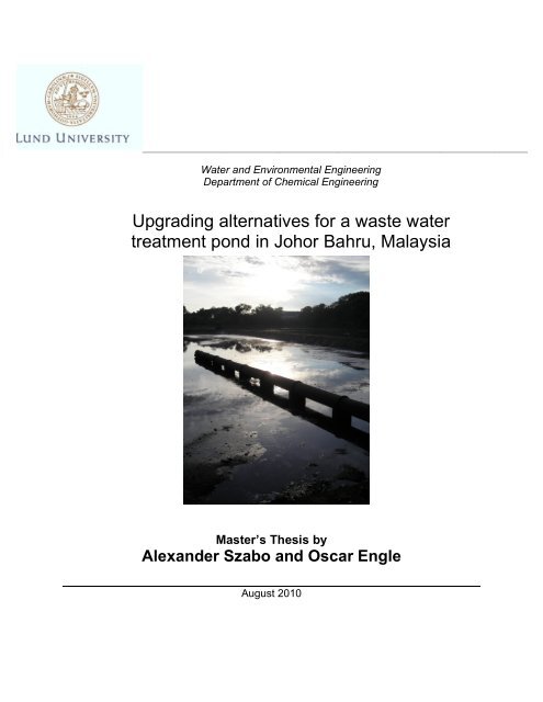
Upgrading alternatives for a waste water 

treatment pond in Johor Bahru, Malaysia 

Master’s Thesis by 

Alexander Szabo and Oscar Engle 

August 2010 

  

 

  

 

__________________________________________________________________ 

Vattenförsörjnings- och Avloppsteknik 

Institutionen för Kemiteknik 

Lunds Universitet 



Lund University, Sweden 

Upgrading alternatives for a waste water treatment 

pond in Johor Bahru, Malaysia 

Master Thesis number: 2010-13 




April 2010 

Supervisor: Associate Professor Dr. Karin Jönsson 

Co-Supervisor: Associate Professor Dr. Azmi Bin Aris 

Examiner: Professor Jes la Cour Jansen 

Picture on Front Page: 

Inlet distribution pipe at Treatment Pond during de-sludging operation, UTM, Johor Bahru, Malaysia. 

_________________________________________________________________________________ 

Postal address: Visiting address: Telephone: 

P.O. Box 124 Getingevägen 60 +46 46-222 82 85 

SE-221 00 Lund +46 46-222 00 00 

Sweden 

Telefax: 

+46 46-222 45 26 

Web address: 

www.vateknik.lth.se 

  

 

  

 

List of abbreviations 

BOD – Biochemical Oxygen Demand 

CFU – Coliform Forming Units 

COD – Chemical Oxygen Demand 

DO – Dissolved Oxygen 

HRT – Hydraulic Retention Time 

IWK – Indah Water Konsortium 

MLSS – Mixed liquor suspended solid 

P.E. – Population Equivalent 

UTM – Universiti Teknologi Malaysia 

TSS – Total Suspended Solids 

WSP – Waste Stabilization Pond 

i  

 

ii  

 

Summary 

Malaysia is developing fast and is striving to become a fully developed country by 2020. After 

independence in 1957 from Great Britain, Malaysia has gradually set up goals for its waste water 

management, which often goes together with economical development and growth. Most of the waste 

water treatment facilities built so far have been made simple and in form of treatment ponds, septic tanks 

and low flushing latrines. In this project a treatment pond at UTM in Johor Bahru has been analyzed. At 

present, the management of UTM is not satisfied with the treatment efficiency and is looking for options 

to upgrade the pond or replace it with an activated sludge system. The objective of this study is to propose 

an upgraded waste water treatment facility to the current treatment pond. 

The treatment pond consists today of two parallel lines, each line with a facultative pond followed by a 

maturation pond. After treatment the water is discharged to a stream close to the treatment pond. At two 

occasions in November 2009 and one occasion in January 2010 sampling and flow measurements were 

performed at the treatment pond. During each occasion sampling and flow measurements were made 

every second hour for 24 hours. This was made to get the characteristics and behavior of the waste water 

quality and the waste water flow. The samples were analyzed and the amount of Chemical Oxygen 

Demand (COD), Biological Oxygen Demand (BOD) and Total Suspended Solids (TSS) were measured. 

The analysis of the data shows that the concentration of COD, BOD and TSS is low. It seems there is a 

significant infiltration into the sewer network at UTM. This was confirmed by the flow measurements 

done at the inlet into the treatment pond. During rain events the influent flow is more than doubled and 

this is something that must be considered when dimensioning a new treatment facility. It seems there is a 

possible misconnection between the stormwater network and the sewer network at UTM. During these 

peaks, the concentration of COD is more than doubled compare to the average COD entering the 

treatment pond. The high COD-values are confirmed by higher TSS values during these rain events. The 

exact reason for this is unknown but one possible explanation could be that the increased flow in the 

waste water pipes will catch and carry with it deposits from the sewage pipe. Another explanation could 

be that somewhere a stormwater channel is connected to the sewer pipes and the stormwater is carrying 

organic material from the ground into the pipes which ends up in the treatment pond. 

At late night the COD value is low but there is still a significant influent flow. This leads to the 

conclusion that the pipe is also taking in groundwater. Together with the increased influent flow during 

rain events and the high flow at night, the total infiltration is estimated to 60-90% of the total influent 

flow. 

From the data collected and analyzed three different solutions for better treatment efficiency have been 

proposed. One solution is an activated sludge system; another is upgrading the current pond by 

rearranging the water flow so that it flows in a series through all four treatment ponds. The third 

alternative is to add aeration to the upgraded treatment pond as calculations shows that the area is not 

sufficient and therefore it is overloaded. A review of the sewer and stormwater network should also be 

considered in order to find the possible misconnection between the stormwater and the sewer water. 

iii  

 

According to assumptions and calculations the activated sludge system will give the best treatment 

efficiency in terms of BOD, nitrogen and phosphorous removal. An activated sludge system will achieve 

standard A requirements according to Malaysian recommendations and according to Malaysian standard 

the activated-sludge system will have an footprint area of around 1 ha if the system receives water from 

more than 10 000 people. The current pond received waste water from around 10 500 people at the time 

this report was written. 

The treatment technology will however be comparatively expensive to build and run. An activated sludge 

system is also less effective, compared to the other suggested alternatives, in removing pathogens and 

there may be a need for some pathogen removal device after activated-sludge treatment. 

The second suggestion to upgrade the current treatment pond does not achieve the same treatment 

efficiency as the activated sludge system. On the other hand it is less expensive to run and easier to 

maintain. It will also reduce pathogens more effectively than an activated sludge system. According to 

assumptions and calculations it will be wise to install oxygen generators as the upgraded treatment pond 

system is overloaded and the oxygen the algae produce is not sufficient for organic breakdown. If 

conservative assumptions and calculations are made the treated water will barely fulfill the requirements 

for Malaysian standard A, but at a low price. If optimistic assumptions are made, the treatment result will 

reach down just below standard A. 

Our recommendations are for financing reasons and for simplicity to keep the old treatment plant, 

improve it by installing screening, installing aeration and baffles and redirecting the flow from parallel 

flow to serial flow through all four treatment ponds. 

iv  

 

Acknowledgements 

This report is a result of a project which has been carried out both in Sweden and in Malaysia. In Sweden 

we were part of the Water and Environmental Engineering at the Department of Chemical Engineering 

where we started and completed our project. In Malaysia where the field study of our project was 

performed we were part of the Environmental Engineering at the Department of Chemical Engineering 

(IPASA). 

We are proud to participate in the cooperation between LTH in Sweden and UTM in Malaysia. We are 

only the “second generation” of Swedish students going away to this friendly and multicultural country. 

Therefore we would like to give our sincere greetings to Prof. Dato’ Ir. Dr. Zaini bin Ujang for 

introducing us to his university from his guest lectures in Sweden, spring 2009. 

A warm thanks goes to our supervisor in Sweden, Ass. Pr. Karin Jönsson, for her professional support 

and guidance during the whole project. Your help and feedback has made this project a lot easier and the 

project would not have been possible without your co-operation between LTH and UTM in Malaysia. 

We would like to give our supervisor in Malaysia Ass. Pr. Azmi Bin Aris our sincere greetings for his 

relentless help at IPASA in Malaysia. Your help and support at UTM was necessary for us in a 

completely new country and environment. We hope to see you again in the future, both in Malaysia and in 

Sweden. 

We are also very grateful to Civ. Eng. Rozlan Md Shariff for his support with maps and data of the 

treatment pond. A special thanks goes to PhD student Chow Ming Fai at IPASA for his help and support 

at the laboratory. We thank PhD student Mohd Noor Asyraf bin Amirruddin for his help with 

precipitation data from the university area. Another special thanks goes to the staff at IPASA for your 

service and helpfulness when we needed it the most. 

We are grateful to our examiner Prof. Jes la Cour Jansen for his useful viewpoints during our project. 

We wish to express our warm gratitude to Prof. Dr. Zulkifli Yusop for professional help and for 

introducing us further into the Malaysian gastronomy with its very tasteful dishes, especially the Satay 

chicken. 

Finally, we would like to thank Ångpanneföreningen, Helsingkrona nation, Rotary Ängelholm and 

Lundabygdens sparbanks stiftelse for your financial support. Without your help this project would never 

had been possible to carry out. 


Lund, April 2010 

v  

 

vi  

 

Contents  

List of abbreviations...........................................................................................................................................iii 

Summary.............................................................................................................................................................iii 

Acknowledgements .............................................................................................................................................v 

1. Introduction ...................................................................................................................................................12 

1.2 Background .................................................................................................................................................12 

1.3 Objective......................................................................................................................................................15 

2. Waste Water Treatment Ponds Technology...............................................................................................16 

2.1 Introduction to Waste water treatment ponds ...........................................................................................16 

2.2 Pretreatment.................................................................................................................................................17 

Screening ...................................................................................................................................................17  

Grit removal ..............................................................................................................................................17  

2.3 Pond Types ..................................................................................................................................................17 

Anaerobic ponds .......................................................................................................................................17  

Facultative Ponds......................................................................................................................................18  

Maturation ponds ...................................................................................... Error! Bookmark not defined.  

Mechanically aerated ponds ..................................................................... Error! Bookmark not defined.  

2.4 Degradation processes ................................................................................................................................18 

Removal of pollutants in Waste water treatment ponds ......................................................................18  

Aerobic degradation .................................................................................................................................18  

Anaerobic degradation .............................................................................................................................19  

Sedimentation...........................................................................................................................................19  

Disinfection................................................................................................................................................19  

3. Pond Hydraulics ............................................................................................................................................21 

3.1 Retention time .............................................................................................................................................21 

3.2 Complete-mix model ................................................................................ Error! Bookmark not defined. 

3.3 Plug flow.................................................................................................... Error! Bookmark not defined. 

3.4 Dispersed flow........................................................................................... Error! Bookmark not defined. 

3.5 Hydraulic design ....................................................................................... Error! Bookmark not defined. 

Short Circuiting........................................................................................... Error! Bookmark not defined.  

Building several ponds in series................................................................ Error! Bookmark not defined.  

Baffles ......................................................................................................... Error! Bookmark not defined.  

vii  

 

4. Activated sludge process technology......................................................... Error! Bookmark not defined. 

Introduction to activated sludge process technology............................. Error! Bookmark not defined.  

Primary treatment ..................................................................................... Error! Bookmark not defined.  

Biological treatment .................................................................................. Error! Bookmark not defined.  

Nitrification and denitrification ................................................................ Error! Bookmark not defined.  

Chemical treatment ................................................................................... Error! Bookmark not defined.  

Activated sludge system – arrangements ................................................ Error! Bookmark not defined.  

Sludge treatment ......................................................................................................................................21  

5. Previous studies on WSP systems...............................................................................................................23 

5.1 Example of computer simulation of WSP geometry ................................................................................23 

5.2 Facultative and maturation ponds in Sri Pulai, Johor Bahru, Malaysia. .................................................25 

5.3 Previous Study on the studied treatment pond at UTM............................................................................26 

6. Study Area ....................................................................................................................................................27 

6.1 Climate.........................................................................................................................................................27 

6.2 The waste water treatment facilities at UTM ............................................................................................27 

6.3 Recipient......................................................................................................................................................28 

Introduction...............................................................................................................................................28  

Sampling procedure for lake water .........................................................................................................29  

Results and discussion ..............................................................................................................................30  

7. Sampling and analysis methods ...................................................................................................................31 

Sampling and flow measurements....................................................................................................................31 

COD ...................................................................................................................................................................31 

BOD 5 ..................................................................................................................................................................32 

8. Water flow and quality .................................................................................................................................37 

Sampling procedure for effluent water...................................................................................................37  

De‐sludging conditions .............................................................................................................................37  

BOD 5  and COD in effluent.........................................................................................................................37  

TSS in effluent ...........................................................................................................................................38  

Average effluent values............................................................................................................................40  

Algae in effluent........................................................................................................................................40  

Reduction in pond system........................................................................................................................40  

Survey of waste water producers at UTM campus ................................................................................41  

viii  

 

Waste water production in the catchment area ....................................................................................42  

Water velocity measurements.................................................................. Error! Bookmark not defined.  

Influent water flow ...................................................................................................................................45  

Total influent water flow..........................................................................................................................46  

Infiltration..................................................................................................................................................46  

Conclusions concerning infiltration .......................................................... Error! Bookmark not defined.  

Sampling procedure for influent water...................................................................................................48  

BOD 5  and COD in influent water..............................................................................................................48  

Total Suspended Solids in influent water................................................................................................50  

Dimensioning values.................................................................................................................................51  

Degradation rate of BOD ..........................................................................................................................53  

9. Proposals for upgrading of the treatment system........................................................................................56 

Alternative 1: Upgrading of existing WSP......................................................................................................56 

Alternative 2: Upgrading of existing WSP – Partly aerated pond ............... Error! Bookmark not defined. 

Alternative 3: Conventional activated-sludge treatment plant ..................... Error! Bookmark not defined. 

Screening device ........................................................................................ Error! Bookmark not defined.  

Grit chamber .............................................................................................. Error! Bookmark not defined.  

Equalization tank........................................................................................ Error! Bookmark not defined.  

Primary settling tank.................................................................................. Error! Bookmark not defined.  

Activated sludge tank ................................................................................ Error! Bookmark not defined.  

Secondary settling tank ............................................................................. Error! Bookmark not defined.  

Sludge handling.......................................................................................... Error! Bookmark not defined.  

Sludge to energy ........................................................................................ Error! Bookmark not defined.  

Disinfection................................................................................................. Error! Bookmark not defined.  

10. Discussion on the upgrading alternatives ................................................ Error! Bookmark not defined. 

11. Conclusion................................................................................................. Error! Bookmark not defined. 

12. Future work ............................................................................................... Error! Bookmark not defined. 

13. References ................................................................................................. Error! Bookmark not defined. 

14. Appendix ................................................................................................... Error! Bookmark not defined. 

  

ix  

 

x  

 

XI  

 

1. Introduction 

1.2 Background 

Malaysia is developing rapidly and the government has set up goals for becoming a fully 

developed country by 2020. This will put more strains on the environment and the keyword is 

therefore sustainable development (Liew, 2008). With an increasing population and a more waterdemanding 

society more waste water is produced. Waste water can have a negative impact on the 

population, the economy and the environment if it is not managed in a wise way. Therefore 

Malaysia is trying to develop a system for waste water handling which is both sustainable and 

suitable for the country’s specific conditions. The complexities and unique environment of 

Malaysia prevent the adoption of a “carbon copy” development that has been successful in other 

countries. 

Malaysia is considered to be a good case study example for other developing countries because of 

its many experiences with different waste water solutions. The government and the authorities 

have tried to implement decentralized on-site systems such as septic tanks and latrines in rural 

and semirural areas. Other implemented systems have been centralized conventional treatment 

plants in urban areas (Ujang & Henze, 2006). The development of institutions and financial 

solutions for waste water systems in Malaysia could also serve as a good study example for many 

developing countries. 

The first sewerage policy in Malaysia was created during the British occupation at the end of the 

19 th century. During this period the so-called Sanitary Boards were organized in Malaysia’s major 

cities and provided services like water supply, latrines, irrigation etc. The Boards were however 

only responsible for waste water and sanitary problems concerning British settlers (Ujang & 

Henze, 2006). After Independence in 1957, sewerage facilities were administrated by the 

Environmental Health and Engineering unit. The unit belonged to the Ministry of Health created 

in the 1960’s (Ujang & Henze, 2006). The unit initiated a successful program in which pour-flush 

latrines were implemented in rural and semirural areas. A pour-flush toilet utilize small amounts 

of water (around 2-3 litres) to pour down human excreta deposit in a pit latrine (UNEP, n.d.). The 

excreta are poured down into a tank where the organic material is decomposed. The sludge 

collected in the tank has to be emptied on a regular basis. 

Pour-flushed toilets were also installed in urban areas but in these areas the unit tried to adopt a 

more conventional sewage approach found in the industrialized world. Due to a lack of finances 

and a well developed national framework for waste water management the implementation was 

slow. In many cases the drawings and plans for the treatment plants remained on the bookshelves. 

A significant step in Malaysia’s waste water management was taken in 1974 when the 

government established the Environmental Quality Act which was the first national legal 

framework for regulating the quality of effluent water from sewage and industries (Ujang & 

Henze, 2006). In 1980 the Malaysian Parliament implemented a new law where developers of 

new housing areas with more than 30 houses were required to provide proper sewage treatment. It 

was favored to keep the new treatment facilities as simple as possible. In order to keep the 

  

12 

treatment facilities simple, treatment ponds or Imhoff tanks were usually implemented. The idea 

was that after one year of utilization, the responsibility for running and maintaining the treatment 

facilities was transferred to the municipal authorities. However, not every local authority had the 

resources to run the centralized treatment facilities and as a result centralized treatment systems 

grew only from 3.5% in 1970 to 5% in 1990. This can be compared to septic tanks coverage in 

urban areas which grew from 17.2% in 1970 to 37.3% in 1990 (Ujang & Henze, 2006). 

In 1993 a new law, the Sewage Service Act, was implemented and a new Federal agency, the 

Sewage Service Department was established. The main task of the new agency was to plan, 

regulate and control sewage water treatment. Since 1993 the agency has been responsible for the 

national privatization project and in 1993 Indah Water Konsortium (IWK) was given the task to 

operate and maintain existing treatment facilities (Ujang & Henze, 2006). The reason for 

privatizing was to assist the Sewage Service Department with maintenance of existing sewage 

systems, refurbishment of old systems and constructions of new sewage systems in urban areas 

(Ujang & Henze, 2006). 

At the moment there are two standards for treated waste water quality, according to the 

Environmental Quality Act from 1974. Every treatment system must comply with either standard 

A or standard B. Standard A is used if the water is discharged upstream of any raw water intake 

and Standard B is used when water is discharged downstream of a raw water intake (Sewerage 

Services Department, 1998). The most important parameters of treated waste water to be 

followed are Biochemical Oxygen Demand over a period of 5 days (BOD 5 ) and total suspended 

solids (TSS). No discharge of treated waste water higher than the absolute values are permitted by 

the law. Because of fluctuations in the quality of the treated waste water, the effluent waste water 

quality should be designed to reach a lower “design” value (Table 1.1). This is to ensure that the 

effluent waste water quality never reach above the absolute values. The permitted limits for 

Standard A and Standard B can be seen in Table 1.1 below. 

Table 1.1: Malaysian Design values for BOD 5 and TSS for treated effluent waste water quality. (redrawn 

from Sewerage Services Department, 1998) 

Parameter Standard A Standard B 

Absolute Design Absolute Design 

BOD 5 (mg/l) 

TSS 2 (mg/l) 

20 10 

50 20 

50 20 

100 40 

During the project the effluent standard from 1974 was changed. It came to our knowledge after 

all the sampling from the pond was done that a new standard was introduced in December 2009. 

The new standard is similar to the one of 1974. The permitted limits for BOD 5 and TSS levels are 

unchanged. The main difference is the introduction of nitrogen and phosphorous removal 

(Department of Environment, 2009). Because no measurements of nitrogen and phosphorous was 

not done we will mostly use Standard A and Standard B from 1974 throughout the report. For 

more information about the new effluent standard see Table C.1 in Appendix C. 

  

13 

In this project, a treatment pond built in 1985 at the Universiti Teknologi Malaysia (UTM) has 

been studied. Figure 1.1 below shows where UTM is situated. The treatment pond was originally 

built for a population of 8 000 P.E. but is currently treating waste water from around 10 500 P.E. 

from the university area. The treatment pond consists of two parallel lines each treating equal 

amounts of waste water. The treated water is discharged to a small stream next to the treatment 

pond. The current discharged waste water is not complying with Standard A according to 

Malaysian requirements. At the moment the pond is only complying with standard B quality 

which is a lower quality standard for treated waste water. The university would like to upgrade 

the treatment facility so that it can comply with Malaysian Standard A requirements as the water 

downstream is used for canoeing by UTM students. The idea is that a new treatment facility could 

also be used for educational purposes for students from the university. Moreover, an improved 

treatment facility at the university also goes hand in hand with Malaysia’s national goals to reach 

a more effective and better management of waste water. 

In order to get a deeper understanding of the water quality and its flow characteristics to the 

current treatment pond, sampling and different kinds of measurements have been performed. The 

obtained information is important as the result of the samples and measurements will be used as a 

basis when designing an improved and more effective treatment facility. 

Figure 1.1: Map of Malaysia and the location of UTM, Johor Bahru. (Reuterwall & Thorén, 2009) 

  

14 

1.3 Objective 

The objective of this master thesis project is to propose and evaluate upgraded waste water 

treatment facilities which can improve the treated effluent waste water quality at Universiti 

Teknologi Malaysia. A new treatment facility should have a footprint area of 25% compared to 

the present treatment pond, as the area around the current treatment pond is planned for 

recreation. The upgraded treatment facilities must also be able to perform a better treatment of the 

waste water compared to the system used today. The requirement is that the effluent can comply 

with an effluent of Standard A quality according to Malaysian directives. 

  

15 

2. Waste Water Treatment Ponds Technology 

2.1 Introduction to Waste water treatment ponds 

Waste water treatment ponds are used around the world for treatment of municipal waste water. 

They can offer a good alternative where land prices are low and where the climate is beneficial. 

Since there is a general relationship between growth rate of bacteria and algae that contribute to 

the treatment of waste water, pond systems in a warmer climate benefit from high temperatures. 

A pond system can be built easily and does not require much maintenance. Since it can hold large 

quantities of water, it has a good resistance to shock loads and hazardous substances that may 

enter the system. 

A typical arrangement of waste water treatment ponds consists of a primary facultative pond 

followed by one or multiple maturation ponds. Under some conditions it is also possible to use an 

anaerobic pond before the facultative pond (see Figure 2.1). 

Figure 2.1: In this figure three possible arrangements for pond system are illustrated. The first two 

series illustrates a primary facultative pond (F) followed by one or two maturation ponds (M). The 

third pond series illustrates an anaerobic pond (A) followed by a facultative pond and finally a 

maturation pond (Szabo & Engle, 2010). 

  

  

  

  

  

  

  

16 

2.2 Pretreatment 

  

Screening 

The purpose of a screening device, which is located before the treatment pond, is to remove 

coarse materials like pieces of plastic and woods etc. The material caught and removed from the 

screen is often of inorganic characteristics and hard to break down biologically in the treatment 

pond. The coarse material can also damage pumps and aerators used in the subsequent treatment 

stages. 

It is recommended that the water velocity through the screen should be less than 1 m/s so coarse 

material will be able to stick between the screens (Mara, 2003). The space between the bars 

should be between 15-25 mm (Mara, 2003). If the flow is above 1000 m 3 /day mechanical screens 

which automatically remove the captured objects should be used instead of screens that have to 

be maintained manually. This is because mechanical screens can be cleaned more frequently. It is 

although wise to have a screen that could be cleaned by hand as a back-up for the mechanical 

screen in case the mechanical screen would stop working. The waste products collected from the 

screen can be taken to the nearest landfill or be incinerated. 

Grit removal 

Grit is made up of heavier and smaller particles (often of inorganic characteristics) like glass, 

sand eggshells etc. Grit can damage pumps and aerators in the subsequent treatment steps and 

should be removed before the treatment pond if the waste water contains large quantities. 

Before water enters the screen and the treatment pond, the waste water may flow in long grit 

channels where the water passes through at a desired velocity. The heavier grit particles will settle 

in the channel as the waste water flows through. The grit channels are made up of two parallel 

channels so one of the channels can be closed for grit removal. A possible problem with a grit 

channel is that it is difficult to keep the velocity at a constant level (Mara, 2003).     

2.3 Pond Types 

Anaerobic ponds 

Anaerobic ponds operate without the presence of algae or oxygen, and have an advantage over 

the facultative pond since they can deal with higher organic loading. They can reduce the organic 

load by 40 to 70% with a retention time of only a few days (Shilton et al., 2005). 

Methane (CH 4 ) and sulphide (H 2 S) are gasses that are produced under anaerobic conditions. 

Methane gas may be considered as a fuel resource if collected, but if not collected as a 

greenhouse gas, contributing to the climate change as it escapes into the atmosphere from the 

pond. If sulphide is produced and released, it is not appreciated since it is releases a bad odor. If 

the anaerobic pond is not properly design, or when overloaded, the release of sulphide may be 

problematic for people living in the surroundings (Mara, 2003). This is confirmed by a study at 

Lee Summit WSP, Missouri, where odor nuisance occurred after the load was increased above the 

pond capacity (McKinney, 1968). 

  

17 

Facultative Ponds 

The main features of the facultative ponds are that they are horizontally divided into two layers, 

with and without oxygen presence. In the top layer (down to 20 - 30 centimeters of depth) 

photosynthesis makes micro-algae produce oxygen during daytime, the oxygen is then used by 

aerobic bacteria to degrade organic substrate. Some of the oxygen in the top layer has its origin 

from surface mass transfer, but it has been estimated that more than 80% of the oxygen is 

produced by algae (Shilton et al., 2005). The depth of oxygen presence in the water is changing 

and depends on many factors such as sunlight, water turbidity and organic loading (Shilton et al., 

2005). In the bottom of the pond, no dissolved oxygen is available, which gives anaerobic 

bacteria opportunities to degrade substrate. The retention time of facultative ponds is relatively 

large, up to several weeks. The long retention time and the shallow design, typically depth is 1.5 

meters, make the ponds consume relatively large land areas (Mara, 2003). 

Since the light needed for the algae arrives through the surface, facultative ponds are usually 

designed by surface loading. In temperate climates, algae are more productive in terms of oxygen 

production and the pond may therefore receive a higher loading of BOD. Eq. 2.1 (Mara, 2003) is 

used to calculate the maximum possible BOD loading per area: 

λ = 350∗(rtial-mix system (EPA, 2002). Since the aeration in a complete mix pond keeps large 

quantities of suspended solids mixed in the pond, a following post-settling pond should be 

installed. Partial-mix aeration may be installed into an existing facultative pond to improve the 

overall treatment efficiency. 

2.4 Degradation processes 

  

Removal of pollutants in Waste water treatment ponds 

The nature is capable to degrade human waste water when it is released into waterways. Problems 

occur when the load on our natural environment is bigger than the self-cleansing mechanisms 

available in our lakes and rivers. The more populated the world becomes, the higher the stress on 

our environment. The waste water treatment ponds are cleaning the water using the same 

processes as in nature. The task of the waste water treatment ponds is to optimize and isolate the 

processes, so that the cleaning has been done before the water is released in our waterways. In 

nature several processes are responsible for the treatment of polluted water, and these processes 

should be used and optimized as much as possible. Some of nature’s processes will be discussed 

in this section. 

Aerobic degradation 

When oxygen is present in water, aerobic microorganisms will use oxygen to oxidize organic 

compounds and produce carbon dioxide (CO 2 ), water and biomass (sludge). Since oxygen is 

consumed by the degradation, the process will be limited by the presence of oxygen. If large 

quantities of organic material are to be degraded, large amounts of oxygen must be supported. In 

  

18 

the case of waste water treatment ponds, the algae are the main producers of oxygen (Shilton et 

al., 2005). Since the algae are only present in the upper part of a pond, it is difficult to achieve 

aerobic decomposition through an entire pond. There are however more advanced pond systems 

where algae are mixed through the water to oxygenate larger volumes. In mechanically aerated 

ponds, oxygen is pumped or mixed into the water which will achieve high dissolved oxygen 

levels. The disadvantage of mechanical oxygen support is that it consumes large amounts of 

energy. 

Aerobic degradation in waste water treatment ponds requires larger volumes and a longer 

retention time then the conventional activated sludge-systems, because the concentrations of 

active biomass, containing the microorganisms, are much lower. 

Anaerobic degradation 

When no oxygen is available, anaerobic degradation may occur by anaerobic microorganisms. 

The benefit of anaerobic digestion is that it can deal with highly concentrated waste water and can 

achieve good purification results within short retention times. The process is temperature 

dependent and will, if properly designed, reduce the BOD concentrations by 40% at 10°C, 60% at 

20°C and 70% at 25°C (Shilton et al., 2005). The anaerobic pond should be installed as the first 

treatment step, when the load of waste water is the highest. The high load of organic matter 

would inhibit the presence of algae. A typical anaerobic pond receives more than 3000 kg 

BOD/ha/day, whereas facultative ponds should not receive more than 400 kg BOD 5 /ha/day in 

order to sustain a healthy algal population (Mara, 2003). 

Sedimentation 

Large amounts of settleable and flocculated colloidal materials that enter the pond will settle to 

the bottom of the pond and create a sludge layer as the water speed declines. Independent of 

whether the particles settle in an anaerobic or facultative pond, the environment, within the 

formed sludge layer, will be anaerobic. Even maturation ponds, which are at the last step of the 

treatment, may produce a thin anaerobic sludge layer at the bottom. The sludge layer is broken 

down anaerobically and thickens over time. Gases (methane and carbon dioxide) that result from 

the degradation arises up though the water and escapes into the atmosphere. It is estimated that up 

to 30% of the BOD load disappears as gas (Shilton et al., 2005). 

Disinfection 

There are several factors within a WSP that together contribute to the removal of illness-causing 

bacteria, viruses, worms and protozoan parasites. It is however difficult to exactly evaluate the 

contribution to the disinfection effect from a single factor, since the processes within a WSP are 

both complex and dynamic. Factors that are known to contribute to disinfection are sunlight (UV) 

exposure, pH, temperature, algal toxins, sedimentation and hydraulic retention time (Shilton et 

al., 2005). The WSP:s are generally considered very good at removal of pathogens (Maynard et 

al., 1999). Research about disinfection shows treatment results from 26 WSP:s around the world 

(see Table H.1, Appendix H). The reduction performance of pathogens in WSP systems is 

  

19 

generally better than conventional mechanical treatment combined with activated sludge (George 

et al., 2002). 

Sunlight (UV) is considered to be the most important factor for disinfection (Davies-Colley et al., 

2000). UV disinfection is complex since different wavelengths affects different species in various 

ways. Some reactions with certain species required dissolved oxygen dependent photo-oxidations. 

In these cases, oxygen is crucial for the performance (Davies-Colley et al., 2000). 

  

20 

3. Pond Hydraulics 

3.1 Retention time 

When dimensioning a pond, the water flow behavior is crucial. One of the key parameters is the 

“retention time”, or “hydraulic retention time” HRT, which occurs as a key parameter in almost 

every calculation. The retention time tells us how long the water, on average, stays within the 

pond. The formula for retention time is: 

θ= pollutant concentration (mg/l) 

r is in the form of ammonium (ay be necessary to add. There is also extra sludge produced from 

this method. 

Sludge treatment 

Sludge created from waste water treatment could easily become a public-health hazard if not 

handled properly. What to do with the sludge is today considered as one of the main problems in 

waste water treatment. Still, there are several methods to choose from when selecting 

  

21 

arrangements which can process sludge. A careful selection of the sludge-treatment method has to 

be made, as costs for stabilization, dewatering and disposal of sludge may be higher than the 

operating cost for the activated-sludge treatment (Hammer, 1986). 

In Malaysia facilities for treating sludge are limited and today most of the sludge is treated in 

sludge lagoons or dried on large sludge-drying beds. Only in semirural areas are these methods 

seen as long term solutions. A more long-term solution for urban areas would be to install 

digesters and mechanical dewatering facilities. Then the gas produced from the digestion 

chamber could be captured and utilized as fuel. 

According to Malaysian standards presented in Sewerage Services Department (1998) a sludge 

strategy consists of three main stages: 

Stage 1 – Preliminary treatment and digestion 

Stage 2 – Conditioning and dewatering 

Stage 3 – Utilization and disposal 

In stage 1, the sludge can be thickened in a centrifuge in order to increase the dry-solids content. 

After the sludge has been thickened, it is sent to an aerobic or anaerobic digestion chamber. 

In stage 2, the stabilized sludge is dewatered in a filter press and the dry-solids content in the 

sludge is raised to more than 25% (Sewerage Services Department, 1998). Sludge lagoons or 

drying beds can also be used in rural areas. 

In stage 3, a sludge tank which can handle sludge for more than 30 days must be provided 

(Sewerage Services Department, 1998). The final step is composting or disposal of the sludge. 

The treated sludge can for example be utilized as fertilizers on fields. 

  

22 

5. Previous studies on WSP systems 

5.1 Example of computer simulation of WSP geometry 

In a test which was executed at Alexandria University, Egypt by Abbas et al. (2006), different 

length/width ratios for a WSP were tested in a computer program in order to determine the 

degradation of BOD and the amount of dissolved oxygen. In reality, there are always a lot of 

parameters affecting the treatment pond which the engineers cannot control, for example 

temperature variations, amount of sunlight and wind speed. In the computer model these 

parameters were set to a constant value. The hydraulic model was assumed to be of dispersed 

flow characteristics. 

The influent waste water had the following characteristics: BOD concentration 300 mg/l, DO 

concentration 0.0 mg/l and 150 kg/(ha*day) in surface organic loading rate of BOD. The 

retention time was set to 31 days, the inflow was set to 0.18 m 3 /s and the pond depth to 1.5 meter. 

The water is assumed to move through the pond as completely mixed (Abbas et al., 2006) (see 

chapter 3.2). The simulation was executed for the four different length/width ratios which can be 

seen in Figure 5.1 below. 

  

23 

Figure 5.1: Different shapes of the waste stabilization pond simulated in the computer program 

(Abbas et al., 2006). 

For each shape, simulations were also executed with 2 or 4 baffles. The baffles will change 

parameters such as the retention time and the flow path in the waste stabilization pond. The 

retention time is changed because the water velocity is changed through the pond. In Figure 5.2 

an example of the 4 ponds with 2 baffles can be seen. 

Figure 5.2: A schematic representation of each shape with two baffles (printed with permission from 

Abbas et al., 2006). 

The effluent amount of BOD 5 was calculated for the different length/width ratios L 1 /L 2 =1, 2, 3 

and 4. In the first case, simulations were executed for different length/width ratios with no 

baffles. The same procedure was then done for each shape with two and four baffles respectively. 

In Table 5.1 the values of BOD 5 , DO and water velocity can be seen from the simulations. 

Table 5.1: The amount of BOD and DO in effluent water (re-drawn from Abbbas et al.,2006) 

  

Without 

baffles 

With two 

baffles 

With four 

baffles 

Range of BOD 5 concentration found in effluent water 

(mg/l) 235-252 22-233 13-54 

Range DO found in effluent water (mg/l) 0.26-0.51 6.24-9.96 9.57-10.03 

Range of minimum water velocity (x 10 -3 m/s) 0.002-0.015 0.018-0.91 0.047-0.05 

Range of maximum water velocity (x 10 -3 m/s) 2.69-3.01 3.19-169 105-765 

The analysis of the results shows that the BOD 5 reduction increases significantly by introducing 

two or four baffles. The best removal efficiency of BOD 5 was achieved with four baffles and a 

  

24 

value of 4:1 in length/width ratio. Within each case it was reported that increasing the 

length/width ratio and introducing baffles slightly increases the water velocity and DO in the 

effluent water (Abbas et al., 2006). The conclusion drawn from these data simulations is that a 

pond should have a length/width ratio of 4:1 and at least two baffles. 

5.2 Facultative and maturation ponds in Sri Pulai, Johor Bahru, 

Malaysia. 

An analysis of the performance of a waste water stabilization pond in Sri Pulai, Johor Bahru was 

done in 2002. The treatment system uses a primary facultative pond followed by a maturation 

pond (Ujang et al., 2002). This is the same pond arrangement as used at UTM. The system in Sri 

Pulai serves a population equivalent (P.E.) of 10 327 from a residential area of approximately 0.7 

km 2 . The ponds together cover an area of 17.725 m 2 , with pond volumes of 16.275 m 3 for the 

facultative pond and 10 115 m 3 for the maturation pond. The volume of the facultative pond 

should result in a retention time of about 30 days. Around 40 % of the incoming water is assumed 

to origin from infiltrating ground water (Ujang et al., 2002). 

Table 5.2: Average waste water characteristics at Sri Pulai WSP. The influent results is based on 24 

samples, the results from the effluent facultative pond and the effluent maturation pond is based on 

14 respectively 7 samples. (re-drawn from Ujang et al., 2002) 

  COD (mg O 2 / SS (g/l) NH 4 -N (mg/l) NO 3 -N (mg/l) 

l) 

Influent 

Effluent facultative pond 

446 

139 

146 

48 

23.1 

19.7 

1.5 

1.6 

Effluent maturation pond 

114 

41 16.8 

1.2 

Removal in entire pond 

system 

74% 72% 27% 

20% 

Removal in facultative pond 

Removal in maturation pond 

69% 

18% 

67% 

15% 

15% 

15% 

- 7% 

25% 

Compared with the effluent standard for Malaysia, the treatment process was not sufficient, since 

the total COD concentration of the effluent was on average 114 mg O 2 /l (see Table 5.2). The 

Malaysian effluent standard B is set to 100 mg COD/l (Ujang et al., 2002). 

The authors´ conclusion of the unexpected low treatment efficiency (the pond should be able to 

meet standard B) could partly be caused by hydraulic short-circuiting. The low treatment 

efficiency could also be caused by the specific growth rates of biological degrading bacteria not 

being so temperature dependent as expected. The authors recommended aeration and installation 

of baffles to improve the treatment. 

  

25 

5.3 Previous Study on the studied treatment pond at UTM 

In year 1999, an under-graduate report was produced by Zahari and Zain (Faculty of Civil 

Engineering, UTM) analyzing the same WSP at UTM. The report is written in Malay language, 

and our focus has been on the waste water composition data found in this report. The 

measurements have been conducted without flow measurements, hence, the results only represent 

average values, that is the values were not weighted against the influent water flow. When the 

waterflow into the treatment pond is high, it is likely that more BOD, COD and TSS will end up 

in the pond, and this is not considered in the report. The results from Zahari and Zain can be 

found in appendix A. 

  

26 

6. Study Area 

  

6.1 Climate 

Johor Bahru lies in a tropical region very close to the equatorial line with temperatures ranging 

between 21 to 32°C all year around. The climate is humid with an average relative humidity 

around 90% (Richmond et al., 2007). The precipitation comes in form of short but heavy rain 

showers and the average rainfall in Johur Bahru is around 2400 mm each year (World 

Meteorological organization, n.d.). The rainiest periods are from March to May when Johor 

Bahru is influenced by the southwest monsoon and November to December when the northeast 

monsoon arrives. 

As Johor Bahru lies in a region with a typical tropical climate with heavy thunderstorms, the 

storm water is usually not connected to the waste water treatment systems. This is also the case at 

UTM where the storm water is led through channels and ditches directly to the local rivers. 

6.2 The waste water treatment facilities at UTM 

Within the Universiti Teknologi Malaysia, two waste stabilization pond facilities and two 

mechanical-biological treatment plants are in operation. The pond system this report will focus on 

is located south-west of the UTM campus area (see Figure 6.1) and it is treating the waste water 

from the western part of the catchment area in UTM (see Appendix D). These WSP’s were built 

in 1985. The mechanical-biological treatment plants were built later, as the university expanded. 

  

27 

Figure 6.1: Map over the UTM campus area with (1) The WSP studied in this report (2) another 

WSP within UTM; (3) biological-mechanical treatment plant; (Another campus area and treatment 

plant is located in the north-east, outside the map) (Szabo & Engle, 2010) 

The treatment system that this report will focus on consists of two parallel lines of facultative 

ponds followed by maturation ponds (Figure 6.2). The available documents do not tell for how 

many persons the ponds are dimensioned for, but according to the contractor for de-sludging 

operation, this pond system was built to serve approximately a P.E. of around 8 000. The pond 

system is a simple construction, where the influent waste water is divided in a chamber before it 

enters each treatment line through pipes located under the water surface. The ponds have no 

screening and objects of many different sizes have been seen floating in the pond. These objects 

have a tendency to clog the cannels between the ponds. Since the water level of the receiving 

river is higher than the effluent level, a pumping station is located between the pond and the river. 

The pumps are currently working discontinuously, and during the time when the pumps are not 

pumping, the ponds accumulate waste water beyond the designed water levels. The technical data 

of the pond system can be found in Appendix G. 

Figure 6.2: Shape of pond system with facultative ponds (1) followed by maturation ponds (2) 

(Szabo & Engle, 2010). 

6.3 Recipient 

  

Introduction 

The effluent from the WSP is released into a stream passing through the UTM area (Figure 6.3). 

The stream transforms into two small lakes a few hundred meters downstream, where the main 

entrance to UTM is located (see Figure 6.4). In these small lakes, canoeing activities take place 

which demands good water quality. The part of water that origin from the WSP is large compared 

to the upstream river water. Most of the water in the lakes is therefore considered mainly to be 

effluent water from the WSP. 

  

28 

Figure 6.3: The receiving river. Upstream (left) and downstream (right) of WSP (Szabo & Engle, 

2010). 

Sampling procedure for lake water 

Composite samples were collected consisting of 3 samples upstream and 3 samples downstream 

the WSP on the 14 th of January 2010. The samples were analyzed for COD and TSS according to 

the procedures described in chapter 7. The points where the three composite samples upstream 

and downstream were collected can be seen in 6.4. 

  

29 

Figure 6.4: Map over recipient with upstream collection points (1) and downstream collection points 

(2) (Szabo & Engle, 2010). 

Results and discussion 

  

Figure 6.5: The water quality upstream and downstream of WSP on the 14 th of January 2010. 

The COD and TSS levels are lower downstream of the WSP (Figure 6.5). The stream has not 

received any effluent from any kind of treatment facility before passing the WSP. The initial 

COD may origin from pollution caused by living organisms such as fishes, birds and algae. The 

high TSS increase downstream may be the result of the treated waste water, but also from high 

concentration of algae and bottom sediments stirred up in the stream. 

Due to limitations in time and the cost for COD reagents, focus has been set on influent and 

effluent water. These values are single analyses of composite samples and should only be 

considered to give an indication of the changes of pollution levels in the river. To reach a better 

  

30 

accuracy (the accuracy of a single analysis is low) of the COD and TSS levels upstream and 

downstream of the pond, more sampling is needed. The COD and TSS levels may also fluctuate 

over the time, both upstream and downstream of the pond. 

Another aspect that must be considered is the accuracy of the COD-reagents. The accuracy and 

precision with Hach’s COD tests are around 5-10% and can be even higher if the sample contains 

suspended solid (Boyles, 2007). It is possible that the sample analyzed from the stream contained 

suspended solids (particle size of 1-100 µm). 

  

  

  

  

7. Sampling and analysis methods  

Sampling and flow measurements 

The sampling procedure included filling plastic containers (each about 1 liter of volume) with 

sample water from the influent chamber and one container with water from the effluent channel. 

The samples were immediately transported to the laboratory where they were stored in a cooling 

room (temperature between 10-13 °C).The following day the analyses of BOD and COD was 

started. TSS analyses were usually carried out a few days after the sampling. The procedure for 

flow measurements is described in Chapter 8. 

COD 

COD analyses have been undertaken with Hach standard procedure for colorimetric 

determination. The Hach reagents used were capable of “high range” (0-1500 mg COD/l). The 

digestions of the reagents were done in a Hach DRB 200 for 2 hours at 150 °C (see Figure 7.1). 

The analysis has been done with single samples. 

The reading of the Hach COD reagents was done in a Hach DR/4000 and a Hach DR/5000 (see 

Figure 7.1). The average values from both machines were calculated. 

  

31 

colorimetric 

Figure 7.1: Hach DRB 200 Digestor for reagents (left) and Hach DR/5000 for 

determination (right) (Szabo & Engle, 2010). 

If the reading showed unexpected low or high values for a specific sample, a new analysis on that 

sample was done the following day. If the new analysis gave the same result, the average of these 

values was used. If another value, that was in the same range as the other samples from that 

measuring event, was measured, that value was used instead. 

BOD5 

Influent samples from the 5-6 November were successfully analyzed by the incubator method. 

The effluent samples from that day were analyzed by the manual method due to lack of available 

space in the incubator. Samples from the other testing events failed due to technical problems, or 

are not used as they are considered unreliable. 

Incubator method 

  

32 

BOD analyzes were carried out using a BOD incubator (Hach, model 205) which is especially 

designed for BOD tests. The sampling bottles are connected with a tube (for oxygen 

measurements) and put in a compartment that keeps the temperature at 20 °C. A computer 

records the oxygen consumption over time. The procedure was performed according to the 

product manual. One benefit of the BOD incubator is that it allows reading of the oxygen 

consumption (BOD) continuously (instead of only a final measurement after 5 days as the 

“manual” procedure described above). For calculations of the k-value (Appendix E) readings 

were recorded with 0.5 days intervals (Appendix F). 

One full testing event with the BOD incubator was successful. Other testing events failed due to 

technical problems with the BOD incubator or lack of available storage space in the fridge where 

the incubator was. 

Manual method 

The “manual” measuring of BOD 5 is done with the following procedure: 

‐ Filing 300 ml airtight bottles with diluted waste water (The purpose of diluting the 

samples was to reach a DO above 7 mg O 2 / liter, which may be necessary for a 

successful BOD reading after 5 days, as the DO must be above 2 mg O 2 / liter at final 

reading. Dilution 1:1 with distilled water was enough for this purpose). 

‐ Measuring the initial DO level in the samples with a DO meter. 

‐ Storing the bottles in a refrigerator at 20 °C for 5 days. 

‐ Measuring the final DO with a DO meter. 

  

The BOD 5 was calculated as the decrease of DO per liter of water. 

This method was considered as slightly unreliable as the reading of the DO meters was difficult. 

The DO measured DO concentration was not stable over time, hence making it difficult to 

measure the final DO. 

  

  

33 

Total Suspended Solids 

TSS analyses were made by filtering 100 ml of sampling through a microfilter (Whatman, GF/C 

glasfaser microfilter). In order to force the sampling water through the filter, an air compressor 

was used to create low pressure in the bottle receiving the filtered water (see Figure 7.2). The 

filters were measured before and after filtering. To eliminate the weight contribution of water, the 

filters were dried in an oven at around 110°C for one hour after filtering, but before final 

measuring. 

Figure 7.2: Sample water was filled in the upper glass container. The air compressor (right in the 

picture) created a low pressure in the receiving container (containing filtered water in the picture) 

(Sxabo & Engle, 2010). 

  

  

  

34 

  

35 

  

36 

8. Water flow and quality 

Sampling procedure for effluent water 

Effluent samples were collected every two hours from the pond outlet at the 5-6 November, 18-19 

November and 9-10 January. From the samples made COD, BOD and TSS were analyzed. Since 

the ponds have large volumes and the retention time is several days, the effluent quality does not 

change drastically during a time span of a few hours. Therefore, for 5-6 November and 9-10 

January, composite samples were created from three effluent samples under approximately a 6 

hour period. This was done in order to reduce work and costs in the laboratory. The analysis 

procedures are described in chapter 7. 

De-sludging conditions 

The treatment efficiency is dependent on the sludge, since the sludge contains bacteria that 

degrade pollutants in the waste water. If the sludge has been removed recently, the system may 

operate ineffectively due to the lack of bacteria. If however, the sludge has accumulated for a 

long period, the volume of the sludge will reduce the HRT in the pond system, hence making the 

treatment less effective. One can assume that the best treatment occurs somewhere in the middle 

between the de-sludging operations. 

The WSP (north treatment line) was de-sludged after the first measurements were done on the 5-6 

November 2009. During de-sludging one treatment line at a time is closed down. The waste water 

is pumped out and the accumulated sludge from the bottom of the ponds is removed. The desludging 

operation takes a few weeks to be completed and is done with 10 year intervals. On the 

9-10 January 2010, the WSP had been in operation, after de-sludging, for about 2 weeks when the 

samples were collected. The average effluent COD was 64 mg/l before and 58 mg/l after desludging 

(see Figure 8.1 and 8.2). The average BOD 5 for 5-6 November was 39 mg/l BOD 5 on 

average (Figure 8.1). 

Since the samples were collected just before and after de-sludging, the results presented above 

may be slightly higher than during most of the operation time. Zahari & Zain (1999) showed in 

their report an average effluent of 40 mg/l COD (see Appendix A) which is approximately 30% 

better than the results in this report. This could be due to the sludge conditions discussed above. 

BOD 5 and COD in effluent 

The quality of the effluent water is relatively stable (see Figure 8.1 and 8.2). Variations may 

depend on sunlight that changes the concentrations of algae in the surface layer. Another factor to 

consider is the effluent pump that is working discontinuously where the treated waste water is 

released to the small stream when the waterlevel in the ponds has reached a certain level (more 

information about the pumping effect is discussed on page 36). 

  

37 

Figure 8.1: BOD 5 and COD in effluent from the northern treatment line on the 5-6 November 2009 

(before de-sludging). 

Figure 8.2: COD in effluent from the northern treatment line on the 9-10 January 2010 (after desludging). 

TSS in effluent 

The TSS levels are higher and show a different pattern after the de-sludging was carried out. The 

average TSS on the 5-6 November was 37 mg/l (Figure 8.3), but 22 mg/l on the 9-10 January 

(Figure 8.4). The reason for lower TSS values after de-sludging may be caused by many reasons. 

One reason is the fact that if the ponds had high levels of sludge, the volume of water in the 

ponds decreased, hence creating less retention time and higher water flow, which disturbs the 

settling process. If the sludge reaches a high level from the bottom of the pond, the distance 

between the top sludge layer and outlet channel gets narrower and more solid particles may get 

  

38 

stirred up. The algae population may not have developed entirely after the de-sludging, and since 

algae contribute to the effluent TSS values, it could be another possible explanation. 

For the composite value analyzed on the 9-10 January, between 00-04, it can be seen that it is 

significantly lower than the other values from this date (Figure 8.4). One possible reason could be 

that a pump station is located just after the outlet where the effluent samples were taken. The 

pumps are working discontinuously and start when the water reaches a specific height in the 

treatment pond. When the pumps start operating, the effluent water flow increases drastically. 

This causes differences in the water quality and the measured changes of effluent quality over 

time may therefore have been influenced by the unknown pumping pattern. 

Figure 8.3: Total Suspended Solids (TSS) in the effluent on the 5-6 November 2009. 

Figure 8.4: Total Suspended Solids (TSS) in the effluent on the 9-10 January 2010. 

  

39 

Average effluent values 

The average weighted effluent from 5-6 November, 9-10 January and average values from Zahari 

& Zain, (1999) give the total average values seen in table 8.1. The values from the report by 

Zahari & Zain, (1999) may represent “better” sludge conditions in the pond, hence lowering the 

average level of pollutants (data is available in Appendix A). 

Table 8.1: Effluent average values. 

  BOD 5 (mg/l) COD (mg/l) TSS (mg/l) 

5-6 November 39 64 37 

9-10 January 29 58 22 

Zairi & Zain (1999) 16 40 13 

Average 28 54 24 

Algae in effluent 

Algae are present in the effluent and are known to contribute to the effluent COD and BOD. The 

water showed clear signs of microalgae in every effluent sample analyzed. In order to understand 

the contribution of particles to the effluent COD, one test was carried out with filtered and 

unfiltered composite effluent water from 9-10 January 2010 (see Figure 8.5). 

Figure 8.5: Unfiltered and filtered composite effluent water (from all 12 samples 9-10 Jan 2010). 

  

The unfiltered effluent had a COD level of 57 mg/l and the same filtered effluent 27 mg/l. The 

difference between unfiltered and filtered (suspended COD) made therefore up 30 mg/l COD. 

Since it has been observed that the quantity of algae in the effluent is prominent, algae are 

assumed to contribute to a major part of the 30 mg/l COD difference. 

Reduction in pond system 

In Tables 8.2 and 8.3 below the reduction of average COD and average TSS from the samplings 

made on the 5-6 November, 2009 and on the 9-10 January, 2010 is shown. 

  

40 

Table 8.2: Influent (weighted COD average against the influent water flow, see chapter 10.2) and 

effluent COD values. 

Date Influent COD (mg/l) Effluent COD (mg/l) Reduction 

5-6 Nov, 2009 122 64 48% 

9-10 Jan, 2010 113 58 49% 

Table 8.3: Influent (weighted TSS average, see chapter 10.2) and Effluent TSS values. 

Date Influent TSS (mg/l) Effluent TSS (mg/l) Reduction 

5-6 Nov, 2009 63 37 41% 

9-10 Jan, 2010 47 22 53% 

Survey of waste water producers at UTM campus 

Construction drawings over the area were used to identify the sewage pipes connected to the 

WSP. The chief engineer at UTM helped to identify the outer borders of the catchment. The 

amounts of students and staff living and studying/working within the catchment were identified 

by consulting housing and university offices. Some assumptions have been made where no 

information could be found about the number of people living and working in buildings 

connected to the treatment pond (for more information of the estimation of P.E., see Appendix 

B). 

The number of students and staff working within the faculties at UTM were given a P.E. of 0.2 

instead of 1 (Sewerage Services Department, 1998) as they do not consume as much water at the 

faculties as they would have done at home, thus lowering the P.E. value. 

Outside UTM campus there are private family houses where the sewerpipes are connected to the 

studied treatment pond. The number of people living in each household is not exactly known so it 

was estimated that each household consists of 5 family members. 

Other buildings connected to the treatment pond where no information of the number of residents 

could be given were the UTM Main Office and the Mosque. The number of staff in the UTM 

Main Office was assumed to be 500 and the number of people visiting the Mosque could be up to 

3000 people. The P.E. for the people working and visiting the buildings was set to 0.2 in both 

cases (Sewerage Services Department, 1998). 

The water consumption for UTM’s students is based on a value collected from a report by 

Katimon and Demun (2004). The report concludes that the average water consumption for UTM 

is 260 litres/(person*day). This value is higher than the average value of 208 liter/(person*day) 

for the rest of Malaysia (Ithnin, 2007). 

The reason for the higher consumption according to our proposition could be: 

1. Students and staff at UTM have a more water consuming behavior, such as more showering 

and more use of laundry facilities. 

2. Leakage of fresh water from delivery pipes. 

A third proposition by Katimon and Demun (2004) for the higher water consumption at UTM is: 

  

41 

3. Water intensive faculties at UTM, such as the Environmental Engineering Laboratory and 

Marine Engineering Laboratory, consume large quantities of water. 

When estimating the water consumption behavior of UTM the value from Katimon and Demun 

(2004) of 260 litres/(person*day) is initially used. The water consumption and waste water 

production is normally of equal amount if no irrigation occurs. At UTM it was observed that 

washing machines, cooking facilities and students’ laundry in some cases were not connected to 

the sewer network so the final waste water production behavior of UTM will be lower than 260 

litres/(person*day). 

Waste water production in the catchment area 

The pond receives waste water from around 10 500 persons according to the survey (see 

Appendix B). No factories or other similar activities are present within the catchment. Hence, the 

waste water is pure domestic. 

If the value of 260 litres/(person*day) from Katimon and Demun (2004) is used the waste water 

flow into the pond can be calculated: 

=10 500 . . 260 /( ∗ )= 2730 t home at campus. The sampling period 

started at 17:30 on the 5 th of November but unfortunately there were no flow measurements made 

from the first three sample occasions that day due to technical problems. The first flow 

measurement started at 23:00 which can be seen in Figure 8.7. The flow decreased at night and 

increased slightly in the morning. From 13:00 to 16:00 a rainstorm started which can be seen in 

Figure 8.7 in the precipitation data from UTM’s own rain gauge. In connection to the rainstorm 

there was a significant increase of the flow. 

  

42 

Figure 8.8: Above: The water velocity in the inlet chamber for the northern treatment line of the 

WSP system during 5-6 November. Below: Precipitation data at site (UTM weather station data) 

  

Measurements 1819 November 2009  

 “Holiday period”   

The second measurement period was from the 18 th to the 19 th of November. During this period it 

is estimated that approximately two third of the population had left the UTM campus for 

vacation. The monsoon had arrived and there was rainfall almost every day from the beginning of 

November to the beginning of January. The measurements started at 12:30 on the 18 th of 

November and continued every second hour until 10:00 the next day. A rainstorm started at 

around 15:00 on the 18 th of November and continued more than one hour. During this period 

there is a huge increase in the influent flow. When the rain stops the influent flow is decreasing 

rapidly. The flow continues decreasing until late night and starts increasing in the morning. The 

behavior of the influent flow and precipitation data can be seen in Figure 8.8. During this 

measurement, only one line of the WSP was in operation, hence the velocity is the double 

compared to the flow measurements from 5-6 November. 

  

43 

Figure 8.9 (above): The water velocity in the inlet chamber for the southern treatment line of the 

WSP during 18-19 November 2009. Below: Precipitation data at site (UTM weather station data). 

  

Measurements 910 January 2010  

Weekend  

The last flow measurements were made from the 9 th of January to the 10 th of January 2010, during 

the weekend from Saturday to Sunday. The first measurements started at 12:00 a.m. on the 9 th of 

January and continued every second hour to 10:00 a.m. on the 10 th of January. This was the first 

flow measurement period with no rain and thus no significant flow peak connected to a rain 

event. From the afternoon on the 9 th of January the flow decreases gradually and in the evening 

the flow goes up distinctly. The influent flow reaches a maximum at 20:00 and goes thereafter 

down during the night. During the morning on the 10 th of January the flow increases slightly 

again. The behavior of the flow characteristics from this period can be seen in Figure 8.9. 

  

44 

Figure 8.10: The water velocity in the inlet chamber for northern treatment line of the WSP system 

9-10 January 2010. No rainfall occurred during the measurements 9-10 January 2010. 

Influent water flow 

Figure 8.11: The inlet waste water flow to the WSP system. The designed flow is made to fill the gap 

between the measurements during 5-6 Nov. 

* On the 5-6 of November and 9-10 of January, the total flow is assumed to be twice the flow in 

one inlet, since there are two inlets with equal amounts of water. 

* On the 18-19 of November, there was only one line and one chamber in use. However, some 

leakage to the closed line occurred except at the last measurement at 10 a.m., when workers 

managed to stop the leakage. The leakage was measured to 9 l/s and is considered when 

calculating the flow from 18-19 November. 

  

45 

Total influent water flow 

The total inflow for 5-6 November has been calculated with Eq. 8.5 where the peak-flow during 

the rain is included and Eq. 8.6 where the peak-flow during the rain is excluded. The total inflow 

for 18-19 November has been calculated with Eq.8.7 where the peak-flow during the rain is 

included and Eq. 8.8 where the peak-flow during the rain is excluded. The total inflow for 9-10 

January has been calculated with Eq. 8.5 and since there was no precipitation during this 

measuring period no rain peaks has been considered. Average inflow quantity to the pond each 

day will be based on Q tot with rain from 5-6 November, 18-19 November and Q tot without rain 

from 9-10 January. The results can be seen in Table 8.4. 

Table 8.4: Calculated total influent waterflow into the pond system for one day. *Partly using 

designed values. ** Rainfall peaks excluded (on the 5-6 November designed values are used). 

Date 

5-6 Nov 

Q tot 

With rain 

(m 3 /day) 

6346* 

Q tot 

Without rain 

(m 3 /day) 

5428** 

Q max 

(m 3 /s) 

0.190 

Q min 

(m 3 /s) 

0.039 

Q Average 

With rain 

(m 3 /s) 

0.073* 

Q Average 

Without rain 

(m 3 /s) 

0.058** 

18-19 Nov 

7527 

6617** 

0.203 

0.059 

0.087 

0.077** 

9-10 Jan 

No rainfall 

5526 

0.085 

0.049 

No rainfall 

0.064 

Infiltration 

High infiltration of groundwater into the sewer pipes is a common problem. Sewers may leak 

waste water out of the pipes or infiltrate groundwater into the sewer pipes, depending on the 

water content of the surrounding soil. It has been observed during our measurements that there is 

a flow of waste water even in late night or early morning even during vacation periods. The waste 

water flow drastically increases during rain events, and the waste water strength is weak (diluted). 

This is an evidence of infiltration into the pipes. The extra infiltrating water is mostly unwanted 

since it demands bigger tanks, or ponds, and to some degree will make the treatment less 

effective. However, one benefit is that since the water is already diluted, it may be easier to meet 

the requirements for discharging the water. 

Three different approaches have been used to find the amounts of infiltrating water. 

  

46 

Method 1: Estimation of domestic water consumption 

If one assumes that the average contribution of waste water per capita is 208 l/day, and the 

number of people is known to be 10 500, the infiltration may be calculated (see Table 8.5). 

Table 8.5: Estimation of infiltrating water, taking total water flow and assumed domestic water 

consumption into consideration. **Assumes all inhabitants present. *Assumes only 1/3 of students 

and staff present due to holiday. 

Date 

Measured total 

inlet water 

during 24h (m 3 ) 

Assumed 

Domestic water 

consumption (m 3 ) 

Infiltration (Total 

– Domestic) 

(m 3 ) 

Amount of 

infiltration in 

pipes 

5 – 6 Nov 6346 2184** 4162 66% 

18 – 19 Nov 7527 728* 6799 90% 

9 – 10 Jan 5526 2184** 3342 60% 

Method 2: Calculating base flow and rain peaks 

The lowest flow measured during night times is considered as base flow. At this time (lowest 

flow usually occurred between 04:00 a.m. and 06:00 a.m.) the water is considered to be purely 

infiltrated water. The contribution from rainfall has been excluded according to Eq. 8.5 and Eq. 

8.6 respectively. 

Table 8.6: Calculations of infiltration by using baseflow and peak flow. 

Date 

Measured total 

inlet water during 

24h (m 3 ) 

Total inlet water 

without base-flow 

and rain peak (m 3 ) 

Infiltration 

(Base 

flow+Rainpeak) 

(m 3 ) 

5 – 6 Nov 6346 2028 4318 68% 

18 – 19 Nov 7527 1559 5968 79% 

9 – 10 Jan 5526 1275 4251 77% 

Amount of 

infiltration in 

pipes 

Method 3: Calculating the COD dilution in waste water 

The load per capita is assumed to be 120 g COD per day (Kemira, 2004). With assumed fresh 

water consumption it is possible to estimate the theoretical concentration of COD in the waste 

water. 

  

47 

COD concentration, theoretical=er channels contributes with 60-90% of the total incoming 

water to the WSP. It can be seen on the velocity measurements that soon after the rainfall occur, 

the flow speed increases rapidly. As the rainfall ends, the flow tends to go down quickly. On the 

18-19 of November, most students left UTM for holiday. Approximately one half to two thirds of 

all students were not at the University during these measurements. Despite this, both Q max and 

Q min (Table 8.4) were higher during the holiday than during the school period. This could be 

explained by that the monsoon period started just after the measurements on the 5-6 November, 

but before the 18 th of November. More or less every day received heavy rainfalls which could 

have raised the groundwater level, thus creating more infiltration into the sewer system. Since the 

storm water channels are built to receive all the storm water, no additional water should enter the 

sewage network. If the infiltrated water could be reduced, the HRT in the WSP would increase, 

hence improving the treatment efficiency. An unavoidable effect of reducing the infiltration is the 

increase in concentrations of pollutants in the waste water. It is however preferable to receive 

smaller quantities of waste water, even if the concentrations of pollutants are higher, since with 

effective reduction the total load of pollutants on the recipient will be lower than with diluted 

waste water. 

Sampling procedure for influent water 

The influent water was collected every two hours during the measurement periods. Samples were 

withdrawn from the inlet chamber and immediately taken to the laboratory and stored in a 

refrigerator. 

The first sampling started 5 th November at 17:30 and continued every second hour until 14:15 the 

next day. The second sampling started at 12:30 a.m. on the 18 th of November and continued every 

second hour until 10:00 a.m. the next day. The third sampling started at 12:00 a.m. on the 9 th of 

January and continued every second hour to 10:00 a.m. the 10 th of January. 

From all these samplings days COD, BOD 5 and TSS were analyzed according to the methods 

described in chapter 7. From the samples 5-6 November k-values were analyzed. Since the 

measurements during 5-6 November lacks flow data between 17:30 and 22:00, a designed flow 

was created and used in order to get complete measuring data and to calculate weighted 

parameters (see Figure 8.10). 

BOD 5 and COD in influent water 

The inlet COD concentrations show a tendency to rise when people use water consuming 

facilities at most, usually in the morning and late afternoon. When water flow increases due to 

rainfall, the COD values peaks and reaches levels much higher than during normal flow. At late 

night or early morning (04:00-06:00) all three sampling periods reach their lowest values (12 mg/l 

– 33 mg/l) (Figure 8.11). The pattern of COD concentrations is lower during the holiday period, 

which is explained by the lower load due to absence of students in combination with infiltration. 

According to Mara (2003), a COD concentration of less than 400 mg/l is considered as “weak 

strength”. This water is therefore placed into this category. 

From the first sampling period 5-6 November, BOD 5 from all 12 measurements were analyzed. 

For all 12 measurements that period, COD was also analyzed. This was done in order to get a 

  

48 

atio between BOD 5 and COD for the waste water entering the pond. In Figure 8.12 COD- and 

BOD 5 -values have been plotted. 

Figure 8.12: The inlet COD concentration during three 24-hours measurements. 

Figure 8.13: BOD 5 and COD concentration values in inlet to the WSP during 5-6 November 2009. 

Ratio BOD 5 /COD in Inlet 

By using the samples from the 5-6 November, the average ratio between the BOD 5 and COD 

values are 0.5 (see Table 8.8 below). This value will be used to estimate BOD 5 when only COD 

values are available. 

  

49 

Table 8.8: Measured BOD 5 and COD on the 5-6 Nov 2009. Relationship 

BOD 5 /COD is calculated from average values. The ratio BOD 5 /COD at 05:00 

is not considered because of an invalid value. 

Time:   COD (mg/l) BOD 5 (mg/l) Ratio BOD 5 /COD 

17:00   120   58 0.48 

19:00   77   35 0.45 

22:00   62   36 0.58 

23:00   79   41 0.52 

01:00   72   54 0.75 

03:00   48   29 0.60 

07:00   46   39 0.85 

09:00   126   76 0.60 

11:00   222   63 0.28 

13:00   148   66 0.45 

14:15   195   89 0.46 

            

  Average: 102   51   

      Ratio = 0.5   

Total Suspended Solids in influent water 

  

50 

Figure 8.14: Above: TSS concentrations from all three measurements periods from influent waste 

water to the WSP. Below: Rain data collected from UTMs weather station. It can be observed that 

the TSS on the 5-6 November and 18-19 November are directly affected by the precipitation. 

The TSS trend tends to be highly affected by rainfall (see Figure 8.13). The peak at 08:00 on the 

9-10 Jan is not related to any rainfall and the cause is unknown. The same sample showed an 

unusual high COD-value as well the TSS result is considered as valid. 

Dimensioning values 

TSS 

For all 12 waste water samples collected on 5-6 November 2009, 18-19 November 2009 and 9-10 

January the maximum and minimum TSS-value has been tabulated in Table 8.9 below. From the 

flow data collected an average weighted TSS value and total load per day has been calculated. 

Table 8.9: Measured TSS-values on 5-6 November 2009, 18-19 November 2009 and 9-10 

January 

2010. 

* Partly based on designed flow 

  Maximum Minimum Weighted Total load per 

5-6 Nov 

18-19 Nov 

9-10 Jan 

Average value 

(mg/l) 

150 

210 

193 

(mg/l) 

11 

1 

2 

average (mg/l) 

63* 

52 

47 

54 

day (kg) 

401* 

389 

261 

350 

COD 

For all 12 waste water samples collected on 5-6 November 2009, 18-19 November 2009 and 9-10 

January the maximum and minimum COD-value has been tabulated in Table 8.10 below. From 

  

51 

the flow data collected an average weighted COD-value and total load per day has been 

calculated. 

Table 8.10: Measured COD on 5-6 November 2009, 18-19 November 2009 and on 9-10 January 2010. 

*Partly based on designed flow 

  Maximum (mg/l) Minimum (mg/l) Weighted 

average 

(mg/l) 

5-6 Nov 

18-19 Nov 

9-10 Jan 

Average value 

222 

381 

390 

23 

12 

23 

122* 

112 

113 

116 

Total load per 

day (kg) 

775* 

841 

626 

747 

  

BOD5  

For all 12 waste water samples collected on 5-6 November the maximum and minimum BOD 5 - 

values has been tabulated below. Because there is no data for BOD 5 on 9-10 November 2009 and 

on 9-10 January 2010 the BOD 5 from these measurements are estimated by using the 

BOD 5 /COD-ratio from 5-6 November 2009. From the flow data collected an average weighted 

BOD 5 value has been calculated in order to calculate the total BOD 5 load per day. The values can 

be seen in Table 8.11 on the next page. 

  

52 

Table 8.11: Measured BOD 5 on 5-6 Nov 2009 and estimated BOD 5 on 18-19 Nov 2009 and 9-10 Jan 

2010. 

* Partly based on designed flow 

** Based on estimated BOD 5 -ratio 

  Maximum (mg/l) Minimum (mg/l) Weighted 

average 

(mg/l) 

5-6 Nov 

18-19 Nov 

9-10 Jan 

Average 

  

89 

191** 

195** 

26 

6** 

12** 

59* 

56** 

57** 

57 

Total load per 

day 

(kg) 

371* 

421** 

314** 

369 

Degradation rate of BOD 

K-value used in this report indicates the speed of the BOD degradation. The k-value, in this report 

used for degradation of BOD, is calculated by the increase of oxygen consumption over time. 

Results of the k-value are listed in Table 8.12 below. The k-value data can be found in Appendix 

F. For more information about the k-value see Appendix E. 

Table 8.12: k 20 -values calculated with Thomas method (Thomas, 1950); 

Influent waste water from 5-6 November 2009. 

Time: k-value (d -1 ) 

17:00 

19:00 

22:00 

23:00 

01:00 

03:00 

05:00 

07:00 

09:00 

11:00 

13:00 

14:15 

Average 

k-value 

(d -1 ) 

0.235 

0.144 

0.254 

0.282 

0.256 

0.294 

0.179 

0.289 

0.274 

0.190 

0.255 

0.222 

0.24 

  

53 

  

54 

  

55 

9. Proposals for upgrading of the treatment system 

  

Alternative 1: Upgrading of existing WSP 

The existing WSP has advantages since it does not consume any energy and the required 

maintenance is low. With some, relatively inexpensive adjustments the pond system could 

operate more efficiently. 

Proposed new design 

• Installing screening device 

• Rearranging the water flow 

• Installing baffles in two ponds 

Figure 9.1: Overview over current pond arrangement (left) and upgraded alternative 1 (right) 

(Szabo & Engle, 2010). 

The purpose of rearranging the water flow to one long train of 4 ponds, instead of two parallel 

lines with two ponds in each (Figure 9.1), is both theoretically and practically motivated. The 

theoretical benefit is due to the enhanced plug-flow behavior of water when more ponds are used 

after each other (see Chapter 3.5 and 2.3 - Disinfection). The practical evidence was seen in 

Christchurch (NZ), where a similar rearrangement was done and significant reduction of 

pathogens, BOD and TSS (Masterton District Council, 2009) took place. The benefits of 

installing baffles are discussed in Chapter 5.1. 

  

  

56 

  

Screening device  

The task of the screening device is to separate larger particles from the waste water and protect 

the following treatment steps. The treatment ponds today have no screening device and large 

floating objects have been seen in the pond. Except from being an unpleasant sight at the pond 

(and especially in the receiving river) the larger objects have been observed to clog channels. 

According to the Sewerage Services Department (1998) the screening device should have a 

maximum clear spacing of 25 mm and be automatically raked, since it serves over 10 000 P.E. 

Flow through ponds  

Design values: 

Average temperature for coldest month=26 °C 

(TheWeatherChannel) 

Qinhe inlet water has a BOD degradation rate (k-value) of 0.24 day -1 at 20 °C (see Table 8.12). 

After the first pond the value is 

unknown but may be assumed to 

be 0.1 day -1 (See Appendix E). 

These values must be converted 

for actual site conditions of 29 

degrees Celsius, using equation 6 

from Mara (2003): 

  

57

Alexander Szabo and Oscar Engle - Svenskt Vatten

You also want an ePaper? Increase the reach of your titles

Delete template?

Save as template?