TVM Tutorial - Dr. James R. DeLisle

Tutorial 1: TVM and Six Functions of $1
© JR DeLisle
Introduction to Time Value of Money (TVM)
&
Six Functions of $1
By: James R. DeLisle, Ph.D.
Revised: Fall, 2008
i
© JR DeLisle: Academic Use Only

Tutorial 1: TVM and Six Functions of $1
© JR DeLisle
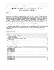
Table of Contents
Preface.......................................................................................................................................... 1
What is this Topic Doing in my Curriculum? .......................................................................... 1
Why Should I Bother? ............................................................................................................. 1
Introduction to TVM .................................................................................................................... 2
The Money-Time Nature of Real Estate .................................................................................. 2
Graphical Depiction/Visualization ........................................................................................... 3
Total Nominal Cost vs. Present Value Cost............................................................................. 4
Present Value Imperative ......................................................................................................... 5
Simple Interest vs. Compound Interest .................................................................................... 6
Mathematical Empowerment ................................................................................................... 8
Analytical Intuition .................................................................................................................. 8
Organization ............................................................................................................................. 9
Overview of 6 Functions of $ .................................................................................................... 10
Basic TVM Terminology ....................................................................................................... 10
Alternative Methodologies for TVM Analysis ...................................................................... 12
Graphical Representation of 6 Functions of $ ....................................................................... 12
Detailed Review of 6 Functions of $1 ....................................................................................... 16
FV1: Future Value of Lump .................................................................................................. 16
FVA: Future Value of Annuity .............................................................................................. 19
SF: Sinking Fund ................................................................................................................... 23
PV1: Present Value of Lump ................................................................................................. 27
PVA: Present Value of Annuity (aka PV1/P) ........................................................................ 30
PR: Periodic Repayment to Amortize $1 ............................................................................... 32
Conclusion ................................................................................................................................. 35
ii
© JR DeLisle: Academic Use Only

Tutorial 1: TVM and Six Functions of $1
Preface
What is this Topic Doing in my Curriculum?
The typical real estate student may feel they are above the level of basic “Time Value of
Money (TVM),” having magically catapulted to the world of canned spreadsheet applications
or commercial discounted cash flow packages. While such tools are readily available, they
cannot be validly and reliably applied without a firm understanding of the underlying
mathematics of real estate finance. This caveat is based on the fact that despite the significant
progress that has been made in standardizing real estate terminology and contracts as a
byproduct of the emergence of the public market, that in reality, real estate remains largely an
inefficient, private market in which transactions are negotiated on an individual basis.
Furthermore, there are a wide variety of economic elements of real estate transactions that
create an overwhelming array of combinations and permutations which can materially affect
the economic viability of a particular investment. While spreadsheets and canned models can
go a long way toward taking the tedium out of running a seemingly infinite array of numbers,
such an approach is both inefficient and ultimately ineffective in arriving at an optimal
solution.
While the previous discussion might suggest that real estate financial calculations are
inherently complex, the reality is that an analyst who understands the nuances of TVM can
arrive at optimal decisions in an efficient manner. Furthermore, no matter who you are or what
background or training you have, you can become an analyst; at least to the extent that you can
master the skills necessary to model the investment performance of real estate opportunities,
both residential and commercial, both individual and portfolio. As you will soon learn, an
understanding of basic TVM can help you win in real estate negotiations, since the literate
party can quickly and intuitively understand the nature and bottom line impact of tradeoffs that
may be placed on the table during negotiations. Furthermore, you can develop an
understanding for the sensitivity of returns to changes in basic assumptions, either in a
particular investment profile, or in the broader economic and investment market in which such
decisions are being made.
Why Should I Bother?
Whether you become a professional whose bread and butter depends on real estate, an investor
who dabbles in real estate, or a user who buys or leases property, you will find the insights and
skills conveyed in this book to be invaluable assets. This claim is especially true when
juxtaposed against the alternative of blindly plugging in assumptions, hoping that they will
produce the desired return or project valuation. While it might seem that mathematical
calculations may be trivial and the answers obvious, the reality is that the underlying elements
can take a number of gyrations that make the quantification of dependent variables extremely
complicated and time consuming. You might be tempted to think that you can avoid the
tedium of beginning with the basics and crunching numbers on a calculator in favor of some
1
© JR DeLisle: Academic Use Only

Tutorial 1: TVM and Six Functions of $1
canned computers packages. If you go down this path, however, you will quickly find that
such trial and error approaches are not efficient. Furthermore, they will not provide you with
the ability to assess the financial risks associated with a real estate opportunity since you will
not have an adequate analytical foundation upon which to model such issues. Thus, if you
allow yourself to remain a naïve user blindly plugging in numbers, you will likely never
develop an understanding of their interactive effects and the unanticipated linkages among
them. Rather, you will be left with a confusing array of outputs that cloud the underlying
economics of an investment or, even more limiting, give you a false sense of security that you
have arrived at the ultimate answer. Then, when things change, as they inevitably will, you
will be forced to start the random process over again, relying on luck to carry you through the
uncertain future.
The Money-Time Nature of Real Estate
Introduction to TVM
By its very nature, real estate is a capital-intensive asset that has both space-time and moneytime
dimensions. That is, the underlying asset includes a number of spatial elements (e.g., site,
building, neighborhood, linkages) that characterize it at a certain point in time, for a certain
time period. At the same time, the money-time element refers to the fact that real estate rights
are typically vested for a specific period of time in return for some income or personal
use/enjoyment that compensates the capital that either acquired or developed the underlying
asset. The duration of these temporal elements is related to the type of control that a party
exerts over the real estate, ranging from a perpetual interest that can be assigned to heirs, to a
lease that creates a tenant interest for a specified term subject to the payment of a certain
amount of rent. Once the magnitude and timing of cash flows can be delineated and return
requirements or interest rates specified, TVM calculations can be used to determine the “value”
of the transaction. Since money has a temporal dimension (e.g., $100 today is worth more than
$100 in 5 years), and decision-makers are usually comparing alternative deals, Present Value
(PV) is typically used to bring everything back to the current time and ensure that alternatives
are compared on an “apples-to-apples” basis.
2
© JR DeLisle: Academic Use Only

Tutorial 1: TVM and Six Functions of $1
Graphical Depiction/Visualization
Given the various combinations and permutations of cash flows surrounding real estate
transactions, and the number of independent items that can affect investments, one of the
challenges analysts face is the ability to visualize the actual pattern of revenues and receipts.
Without this intuitive understanding, it is difficult to set up problems so that they can be solved
in an efficient manner. Fortunately, once the basic elements of TVM are mastered, one can
easily extract the “direction” of changes in a dependent variable (e.g., rate of return, value).
Exhibit 1: The Money/Time Continuum
Money
+
-
Time
T = 0
T = 5
Illustration 1 lays out a basic graphical representation of the money/time relationship. As
noted, time is represented on the horizontal or x-axis; money is represented on the vertical or y-
axis. The Money axis extends from the negative to the positive, with the intersection of the
Time axis establishing the “0” point. The Time axis spans from the past to the future, with the
intersection of the Money axis delineating the “current time” which is also often noted T=0.
The future is generally counted in terms of the number of periods from today; with T=5
suggesting that it is 5 years hence.
While we want to keep this initial discussion simple, it should be noted that there are two
additional temporal elements that will be key in TVM calculations: periodicity, and
beginning/end of period.
• Periodicity. The notion of “periodicity” refers to the number of compounding periods
per year. For example, a periodicity of 1 would indicate annual payments. On the other
hand, a periodicity of 12 would indicate monthly payments (i.e., 12/’year).
• Beginning/End of Period. The beginning/end of period notion comes into play since
there can be significant differences in the value/cost of some exchange of capital
depending on whether it occurs at the beginning of the period (BOP) or the end of the
period (EOP). This is especially true if there is differing from the initial exchange. For
3
© JR DeLisle: Academic Use Only

Tutorial 1: TVM and Six Functions of $1
example if you receive $1,000 at the beginning of the first year, and pay back the future
value at the end of the 5 th year, you have really held onto the capital for 6 years, not 5
years.
• Consistency. In both periodicity and BOP/EOP calculations, the key is to keep the base
consistent to support apples-to-apples comparisons. For example, if you receive 7%
interest, compounded annually, for a 5 year hold you would enjoy 5 steps or earning
periods in your principal plus interest calculations. On the other hand, if you received
7% annual, compounded monthly, you would enjoy 60 steps or earning periods (i.e., 5
* 12). On a similar note, the calculation of holding period costs/benefits should be
consistent, with both inflows and outflows expressed in BOP or EOP bases; they should
not be inconsistent or the number of compounding principles should be adjusted.
Total Nominal Cost vs. Present Value Cost
The fallacies of using nominal dollars can be illustrated with a couple of examples. Take the
case of the purchase of a house that you buy for $240,000 and get a 7.5%, 30 year, fixed rate
mortgage with monthly payments. On a simple level, you might think you are paying $14,440
in interest (i.e., $240,000 * 80% loan to value * 7.5% interest). In reality, you will be making
monthly payments of $1,341 for 360 months. If you own the house for the full term, you will
be making total payments of $483,297. If you subtract the initial loan amount, that is $291,297
in interest alone. If interest rates were 10%, the total payments would balloon to $606,577,
with a monthly payment of $1,685, more than $344 above the 7.5% rate. This elasticity of
payments, especially compared to wages which are less volatile –at least on the upside-- is one
reason that homeowners can get caught with low teaser rate financing on variable rate loans.
Once the loan resets, the jump in payments to the initial rates can be onerous. This situation
can be further complicated if rates rise as can be expected as the cycle unfolds, their ability to
pay may not keep up with interest rates.
Another example can be drawn from a recent effort to defeat a monorail project in Seattle.
After being narrowly approved on two occasions, when another opportunity came up to force a
vote, opponents used total nominal dollars costs to exaggerate the effective cost of the project
on voters. When the aggregate dollars were added up, the apparent cost was daunting, helping
tip the polls toward an eventual defeat. Given the state of infrastructure and the need for
deferred maintenance, it is likely such tactics will continue to be used to defeat future
measures. Unfortunately, since many voters and members of the general public do not
understand TVM, the risk of making sub-optimal decisions on poor economics remains.
Fortunately, those of you who work your way through this material should be in a position to:
1) analyze the true costs of various scenarios yourselves, 2) help educate others on the impact
of TVM on decisions, and 3) develop more creative, cost-effective financial structures to
achieve certain goals and objectives.
4
© JR DeLisle: Academic Use Only

Tutorial 1: TVM and Six Functions of $1
Present Value Imperative
One might question why so much emphasis is placed on Present Value; isn’t it true that dollars
are dollars? While dollars are indeed relatively fungible (i.e., a dollar is a dollar is a dollar,
either paper, silver or some equivalent), the value or purchasing power of a dollar varies
dramatically over time. Since real estate and other investment decisions have a temporal
nature (i.e., they occur or endure for some finite period), to make a correct economic or
financial decision, it is critical that future outflows or inflows be expressed in present dollars.
This is especially true since options often have different time periods and different risks. The
only way to compensate for these differences and inherent uncertainty, is to bring the
economics to a common point in time. Typically, future dollars are brought to the current or
present time, although a fixed future time would be just as valid. The key in such decisions is
to state the economics of various options on an “apples to apples” basis. While non-economic
factors are also typically incorporated in decision making, having the economic elements
expressed in clear and unambiguous terms helps the decision maker focus on other elements or
criteria.
5
© JR DeLisle: Academic Use Only

Tutorial 1: TVM and Six Functions of $1
Simple Interest vs. Compound Interest
Before getting into any detailed TVM discussion, it is important to explore the differences by
compound vs. simple interest since compounding is built into all TVM calculations. Consider
the following example to see the differences.
1 (a): Simple Interest
Using simple interest, our $1,000 would earn $75/period for 5 periods. Thus, the math is
relatively straightforward. Namely,
Total interest = ($1,000 * 7.5%*5yr)
= $375
Future Value = PV + Total interest
Exhibit 2: Simple Interest
= $1,000 + $375
= $1,375
$1,000
Simple Interest
Σ = $375
x 7.5.%
=
$75 $75 $75 $75
$75
6
© JR DeLisle: Academic Use Only

Tutorial 1: TVM and Six Functions of $1
1 (b): Compound Interest
In the case of compound interest, we would earn interest on the interest, compounding forward
to a future lump sum. Thus, the math is a little more complicated since it introduces an
exponential function. Namely,
Table 1 (a): Exponential Equation for Compounding FV
Future Value (FV)
Where:
Present Value
Rate
Compounding Periods
= PV * (1 + r) t
= $1,000 * (1.075) 5
= $1,000 * 1.4356294
= $1,435.63
PV $1,000
r 7.50%
t 5
(Note: Annual Equation; if monthly r/12 and t*12)
Note that we are keeping this example simple by looking only at annual payments so the Term
(t) is the same as the number of compounding periods. In the future, we will denoted the Term
as t, but the compounding periods/year will be denoted as “m.” Thus, if this example was
monthly, the Compounding Periods would be 60 (i.e., 5 * 12)
Table 1 (b): Tabular Example of Compounding PV
Begin
Interest
End
Balance Rate Earnings Balance
1 $1,000.00 7.50% $75.00 $1,075.00
2 $1,075.00 7.50% $80.63 $1,155.63
3 $1,155.63 7.50% $86.67 $1,242.30
4 $1,242.30 7.50% $93.17 $1,335.47
5 $1,335.47 7.50% $100.16 $1,435.63
As noted in Illustration 3 (b), the first $75 is added to the initial amount at the End of the
period, and then earns interest at the 7.5% rate which compounds forward to $80.63. Thus, the
$5.63 is the interest on the interest. That becomes the End of the period balance, and is
compounded forward with the process continuing until the end of the term.
7
© JR DeLisle: Academic Use Only

Tutorial 1: TVM and Six Functions of $1
Mathematical Empowerment
Some of you may be wondering whether it is worth it to waste time playing with numbers and
graphs, contending that real estate is essentially a people business in which the art of the deal
dominates who does what. While the behavioral element is indeed important, the capitalintensive
nature of real estate and its long-term nature quickly rise to the top of the chain in
importance. Indeed, there are countless examples of real estate investors who have lost their
properties and their personal wealth by underestimating the importance of solid financial
analysis. On the other hand, those who have been able to amass and sustain wealth
accumulation over the full real estate cycle have all learned how to manage finances for
individual projects, as well as for real estate portfolios.
Analytical Intuition
In many respects, you have undoubtedly found out that life is a matter of timing and luck;
being in the right place at the right time. This axiom carries over to real estate, although with
one major caveat. Namely, one has to be able to identify a great deal and be mobilized to strike
when the iron is hot. While this might seem obvious, during periods when the market is
extremely active and capital is chasing deals, one can easily be confused by the various
machinations and financial engineering used to make projects pencil out. Examples of such
practices include: bullet-loan financing (e.g., 30 year amortization, 3 year due clause); use of
subordinated or mezzanine financing at higher rates to attract more equity; participating and
convertible loans to increase yields over face rates; negative amortization loans which actually
grow rather than shrink in terms of outstanding balances; and, use of rent spikes in proforma
cash flows to increase paper returns over hurdle rates. In addition, by incorporating more
advanced techniques such as sensitivity analysis and Monte Carlo simulation, which we will
introduce later, one can model the vulnerability of individual assets to various market risks and
economic scenarios. Finally, when individual investments are rolled up into a “portfolio,” one
can manage such risks by applying portfolio management techniques including diversification
and asset allocation. Unfortunately, TVM analysis cannot avoid all such risk exposures,
especially those caused by unpredictable shocks to the system. However, it can go a long way
to avoiding situations that are “accidents waiting to happen.”
The intellectual and mathematical range of analytical skills alluded to in the previous
discussion might be daunting to a novice or one with a passing interest in real estate investing.
The good news is that even the most sophisticated forms of real estate analysis can be reduced
to a manageable number of TVM steps. Thus, while analyzing the previous types of problems
is beyond the scope of this guide, mastering the concepts herein is a necessary condition to be
able to analyze more complex problems. Without such an understanding, it would be
impossible to make fundamentally sound decisions, to independently analyze the true cost of
various options, select the “best option” for yourself when looking at alternatives, or evaluate
the quality of financial advice you get from others. As you will note in this guide, such
fundamentals are relatively straightforward in terms of using based Future Value (FV) and
8
© JR DeLisle: Academic Use Only

Tutorial 1: TVM and Six Functions of $1
Present Value (PV) concepts. By building on this foundation, you will be able to convert future
cash flows of various investment or acquisition option with different magnitudes, patterns and
risks to a common denominator. This denominator can be their true Present Value, or the timeadjusted
rate of return they promise if the assumptions you make are borne out. This latter form
of analysis is especially important in real estate, with its long-term, capital-intensive nature.
Indeed, when purchasing real estate, you are really buying a set of assumptions rather than
mere bricks and mortar. As such, by being able to master basic TVM math and model
alternatives, you can explore options quickly and efficiently. This ability will allow you to turn
your attention to more important issues such as whether the assumptions you make in your
modeling are valid and reasonable. Further, you will be able to apply sensitivity analysis to
determine how stable your conclusions are relative to the various assumptions or possible
changes in market conditions (e.g., increasing interest rates, slowing appreciation in housing
markets) you make in your analysis. The importance of being able to conduct such analysis
can be punctuated by the plight of the legions of recent homebuyers who purchased at the end
of the boom cycle and turned to structured financing, as well as those who converted fixed-rate
loans to adjustable rate loans to tap into home equity and lower payments at the same time.
As you will note in this guide, TVM can help you convert real estate alternatives with a myriad
of confusing and seemingly unrelated options from apples to oranges, to apples to apples. As
such, you will be able to make an objective decision can be made on the merits of the deals
rather than on a confusing set of numbers that have little meaning. You will also note that by
mastering these basics and by cultivating the ability to visualize cash flows and reduce
complex problems into simple, discrete components, you will be prepared to approach a range
of heretofore complicated decisions from a solid analytical perspective. Ultimately, by
applying various decisions models, you will be able to combine the quantitative elements of a
problem with the qualitative elements, allowing you to make logical choices that have a high
probability of satisfying explicit goals and objectives that you establish.
Organization
We have designed this workbook for you, regardless of whom you are and where you come
from. Our intent is to provide you with a solid, incremental approach to the mathematics of
real estate finance and investment analysis. We start with the basics, and then build up to more
sophisticated concepts. To address the needs of those of you who will likely return to this
material for a refresher at some point in time, or to fill in some gap in understanding some of
the more subtle nuances of TVM, we have also taken care to ensure that the materials are
cross-referenced and draw on the same jargon, acronyms and equations. Since learning TVM is
by necessity a participatory sport, we have also compiled a number of examples that can be
used as practice exercises. If you get stuck, you can refer back to the building blocks and/or
visualization processes that can help fill in the missing pieces of your analysis. Welcome to
the wonderful world of real estate finance!
9
© JR DeLisle: Academic Use Only

Tutorial 1: TVM and Six Functions of $1
Basic TVM Terminology
Overview of 6 Functions of $
Illustration 4 provides an overview of the 6 Functions of $. As depicted, 3 functions deal with
Present Value, and 3 functions deal with Future Value. The acronyms and corresponding
definitions include:
• Present Value. The current value of future receipts or payments.
o PV1. The present value of a future lump sum (i.e., single payment) received at
some finite time period assuming a stated discount rate.
o PVA. The present value of a series of equal, fixed interval payments, received
over some finite time period assuming a stated discount rate. This is also
referred to at the PV1/P.
o SF. The series of equal, fixed interval payments received over some finite time
period necessary to grow to a targeted future amount earning a stated rate.
• Future Value. The value of current or prior receipts or payments in the future.
o FV1. The future value a present lump sum (i.e., single payment) received today
will compound to over some finite time period assuming a stated rate of
compounding.
o FVA. The future value of a series of equal, fixed interval payments, received
over some finite time period assuming a stated rate of compounding. This is
also referred to as the FV1/P.
o PR. The series of equal, fixed interval payments that must be made over some
finite time period necessary to amortize a present value earning a stated rate.
10
© JR DeLisle: Academic Use Only

Tutorial 1: TVM and Six Functions of $1
Exhibit 3: TVM All-in-One Six Functions of $
11
© JR DeLisle: Academic Use Only

Tutorial 1: TVM and Six Functions of $1
Alternative Methodologies for TVM Analysis
Before delving into the actual TVM calculations, it should be noted here are a variety of
approaches for analyzing problems including:
• Equations. Applying the actual mathematical equations using a basic calculator
with exponential functions.
• Financial Calculators. Using a “Financial Analyst” type calculator that has the
financial functions and underlying equations preprogrammed.
• Spreadsheet. Using Excel or some other spreadsheet using the raw mathematical
equations or using the built-in financial functions.
While each of these methodologies has advantages and disadvantages, if applied correctly, the
solutions will be the same. Thus, in order to solve problems, one will have to master the chosen
methodology (or be able to follow examples to plug in numbers). However, it should be noted
the ability to merely plug in numbers will only work for basic problems that are presented to
the analyst in a clear, unambiguous manner. While this might appear to be a reasonable
expectation, in reality you will discover TVM problems –especially in real estate—are
generally more complex, involving two or more TVM functions. Thus, in approaching real
estate decisions, an analyst must be able to set up a problem and lay out the pattern of cash
flows including nature (i.e., lump or annuity), amount, timing, and appropriate compounding or
discounting rate. Thus, if you merely learn how to blindly plug numbers into a calculator or
spreadsheet, you will quickly find yourself confounded by all but the most basic problems. On
the other hand, understanding how to dissect a problem statement involving money and time,
and set up a solution will enable you to objectively analyze the most complex problems. The
balance of this guide and related cases, lecture, tutorials, and interactive problems are designed
to help you cultivate this understanding. Due to the relationships among the 6 Functions of $,
you will find a degree of intellectual synergy that will make learning more efficient, and more
robust.
Graphical Representation of 6 Functions of $
To help you understand the relationships among the 6 Functions of a $, it is useful to look at a
standardized set of assumptions. Exhibit 3 depicts each of the 6 Functions using a constant set
of assumptions regarding amounts, rates, and timing which consist of:
• Amount . $1,000 for Lump or $200 spread over 5 payments for Annuity (i.e., $1,000/5)
• Term. 5 years
• Periodicity. Annual
12
© JR DeLisle: Academic Use Only

Tutorial 1: TVM and Six Functions of $1
Exhibit 4 (a): Graphical Representation of 6 Functions of $
FV1
$1,436
PV1
$1,000
$1,000
Reciprocals
$697
Future Value of $1Lum p P V
Present Value of $1 Lump F V
FV1/P
$1,161
$809
PV1/P
$200/P
$200/P
Future Value of $1/Period
Present Value of $1/Period
Reciprocals
Reciprocals
SF
$1,000 $1,000
PR
$172/P
$247/P
Sinking F und to G row to $1
Periodic R epaym ent to Amortize $1
It should also be noted that some of the problems are reciprocals (e.g., FV1-PV1, FV1/P-SF,
and PV1/P-PR). This will be important when you are using Excel to solve problems as the
basic functions will used in multiple application.
13
© JR DeLisle: Academic Use Only

Tutorial 1: TVM and Six Functions of $1
Exhibit 4 (b): Narrative Snapshot of 6 Functions of $
FV1: Future Value of Lump
The FV1 asks the basic question, “What will
$1 invested today grow to if it earns interest at
some stated rate over some finite time period?”
In order to use the function, substitute the
current $’s in the place of the $1, and specify
the Rate and Time.
FV1/P: Future Value of Fixed Payments
(aka FVA: Future Value of Annuity)
The FVA asks the question, “What will $1 in
fixed interval payments invested each period
grow to if it earns interest at some stated rate
over some finite time period?” It differs from
the FV1 in the sense that the amount is
invested in equal amounts at fixed intervals
rather than all up front in one lump sum
payment.
In order to use the function, substitute the
actual annuitized $’s in place of the $1, and
specify the Rate and Time.
SF: Sinking Fund
The SF asks the basic question, “What equal
amount will I have to deposit each period to
grow to some targeted Future Value if it earns
some stated rate over some finite time period?”
It differs from the other functions in that it is
looking forward to earning or accruing to a
targeted amount by making a series of fixed
payments/deposits which are compounded
forward, earning interest on the interest.
In order to use the function, substitute the
actual lump $’s targeted at some point in the
future in place of the $1, and specify the Rate
and Time.
PV1: Present Value of Lump
The PV1 asks the basic question, “What will $1
received in the future be worth in current dollars if it
erodes in value at some stated rate over some finite
time period?”
In order to use the function, substitute the actual $’s
received in the future in the place of the $1, and
specify the Rate and Time.
PV1/P: Present Value of Fixed Payments
(aka PVA: Present Value of Annuity)
The PVA asks the question, “What will $1 received
at fixed intervals receipts be worth today in terms of
current dollars (i.e., purchasing power) if inflation
occurs at some stated rate over a finite time period?”
It differs from the PV1 in the sense that the amount
being eroded is received at fixed intervals rather
than all at the end of the period.
In order to use the function, substitute the actual
annuitized $’s in place annuitized of the $1, and
specify the Rate and Time.
PR: Periodic Repayment
The PR asks the basic question, “If I borrow $1
today, what equal amount will I have to pay each
period to repay that amount plus the interest owed
on the outstanding balance if I pay some stated rate
over some finite time period?” It differs from the
other functions in the sense that it is designed to
provide a return of (i.e., repay) and a return on (i.e.,
interest) over the finite period thus reducing the
balance to zero. This is also known as a fixed rate,
fully amortizing loan.
In order to use the function, substitute the actual $’s
borrowed today in place of the $1, and specify the
Rate and Time.
14
© JR DeLisle: Academic Use Only

Tutorial 1: TVM and Six Functions of $1
In this primer, we will explore a number of set-ups for the calculating the core TVM functions.
In Excel, we will demonstrate the answers using two approaches: 1) prompted functions, and
2) raw built-in functions. At first, you may be more comfortable using the prompts, but as you
get more comfortable, you will find it much more efficient to use the raw functions. To make it
easier to follow, we have named the various TVM inputs using Excel’s naming option. Exhibit
4 (c) presents the names we assigned. They are also presented in the accompanying Excel file.
Exhibit 4 (c): Assigned Excel Names for TVM Equations
15
© JR DeLisle: Academic Use Only

Tutorial 1: TVM and Six Functions of $1
FV1: Future Value of Lump
Detailed Review of 6 Functions of $1
TVM Question. The FV1 asks the basic question, “What will $1 invested today grow to if it earns
interest at some stated rate over some finite time period?” The future value of a $1 is the value of a
present amount of money at some point in the future.
In order to use the function in problem solving with real numbers, just substitute the current $’s in the
place of the $1, and specify the Rate and Time.
Exhibit 5: FV1
As noted in Equation 1, the default assumption for all TVM problems, including FV1 is that
the earnings are compounded forward rather than treated as simple interest. Thus, the key
component of all TVM equations becomes:
(1 + i) t
Where :
“i” stands for the interest rate; this may also be denoted “r” or “R” in some examples.
“t” stands for the Term. Note the Term is adjusted for Periodicity so, if monthly, a 5
year period translates to a “t” of 60 (i.e., 5 * 12).
16
© JR DeLisle: Academic Use Only

Tutorial 1: TVM and Six Functions of $1
Table 2 (a): FV $1
Future Value (FV)
Where:
Present Value
Rate
Compounding Periods
= PV * (1 + r) t
= $1,000 * (1.075) 5
= $1,000 * 1.4356294
= $1,435.63
PV $1,000
r 7.50%
t 5
(Note: Annual Equation; if monthly r/12 and t*12)
Table 2 (b): FV Payment in Advance
Begin
Interest
End
Balance Rate Earnings Balance
1 $1,000.00 7.50% $75.00 $1,075.00
2 $1,075.00 7.50% $80.63 $1,155.63
3 $1,155.63 7.50% $86.67 $1,242.30
4 $1,242.30 7.50% $93.17 $1,335.47
5 $1,335.47 7.50% $100.16 $1,435.63
Table 2 (c): FV1 Equations for Alternative Methodologies
Math
Excel
WebCT
=+(FV_PV)*((1+(FV_i)/(FV_m)))^((FV_t)*(FV_m))
=FV(FV_i/FV_m,FV_t*FV_m,0,-FV_PV)
{a}*((1+({i}/100/{m}))**({t}*{m}))
Table 2 (d): HP Answer to FV1
Factor Code Initial Answer
Compounding/Period m 1
Term t 5
Present Value PV $1,000
Payment PMT $0.00
Future Value FV $1,435.63
Interest Rate I 7.50%
17
© JR DeLisle: Academic Use Only

Tutorial 1: TVM and Six Functions of $1
Method Steps: HP 10BII
• First, clear all by pressing the GOLD key and then the C ALL key.
• Second, tell the HP that you want to work annually by entering 1, pressing the GOLD
key, and then P/YR. (NOTE: this should stay the default from the previous until you
change it; clearing the registers does not affect this default).
• Third, enter 5, press the GOLD key, and then press X P/YR.
• Fourth, enter 7.5, press the GOLD key, and then press Nom%.
• Fifth, enter 1,000, and then press PV. Finally, press FV to solve.
Exhibit 6 (a): Prompted Excel Solutions: FV1
It should be noted that Excel uses the same prompts for calculating the Future Value of a dollar
lump (FV1) and the Future Value of an Annuity (FVA). Within Excel, the difference is
whether the input is the Pv or the Pmt. Thus, it is important to ensure that you are plugging the
inputs into the correct location. In the raw function, each of the variables is delineated by a
comma. Thus, it is important to ensure that you place the respective inputs in the correct
locations. The good news is that Excel highlights the variables in the equation as you plug
them in. Also, the =FV will return a negative number to indicate it is the outlay that
corresponds to the future benefit. It can be converted to a positive by leading with =-FV. The
[(type)] variable allows you to specify whether the payments are made at the beginning or end
of the period; usually, they can be left blank unless the payment is does not follow the defalt or
normal conventions. This is the raw FV function:
Exhibit 6 (b): Raw Excel FV Function
18
© JR DeLisle: Academic Use Only

Tutorial 1: TVM and Six Functions of $1
FVA: Future Value of Annuity
(aka FV1/P: Future Value of Fixed Payment)
TVM Question. The FVA asks the question, “What will $1 in fixed interval payments invested each
period grow to if it earns interest at some stated rate over some finite time period?” It differs from the
FV1 in the sense that the amount is invested in equal amounts at fixed intervals rather than all up front
in one lump sum payment.
In order to use the function, substitute the actual annuitized $’s in place of the $1, and specify the Rate
and Time.
Exhibit 7: FVA
The future value of an annuity ($1/period) is the amount that accumulated by a series of equal
payments at interest over a period of time
Types of FVA Problems
There are two types of FVA problems: payment in advance or at the beginning of each period;
or, payment in arrears in which payments are made at the end of the period.
19
© JR DeLisle: Academic Use Only

Tutorial 1: TVM and Six Functions of $1
FV Annuity in Advance. In the case of an annuity in advance, we would receive the first
payment immediately and the rest at the beginning of each period compounding forward to a
future lump sum.
Table 3 (a): FV Annuity in Advance
or
FV = Sum [R(1+ r) n ]
= $200(1.075) 5 + $200(1.075) 4
+ $200(1.075) 3 + $200(1.075) 2
+ $200(1.075)
FV = R * [((1 + r) t - 1) (1+r))/ r]
= $200*[((1.075) 5 -1)(( 1.075))/.075]
= $200 * (6.2440204)
= $1,248.80
Where:
Periodic Receipt
Rate
Compounding Periods
R $200
r 7.50%
t 5
(Note: Annual Equation; if monthly r/12 and t*12)
Table 3 (b): Annuity in Advance Schedule
Period Period Interest End
Receipt Begin. Bal. Rate Earnings Balance
1 $200 $200.00 7.50% $15.00 $215.00
2 $200 $415.00 7.50% $31.13 $446.13
3 $200 $646.13 7.50% $48.46 $694.58
4 $200 $894.58 7.50% $67.09 $961.68
5 $200 $1,161.68 7.50% $87.13 $1,248.80
FV Annuity in Arrears. In the case of an annuity in arrears, we would receive the payments at
the end of each period compounding forward to a future lump sum.
Table 3 (c): FV Annuity in Arrears
FV
Where:
Periodic Receipt
Rate
Compounding Periods
= R * [ ((1+ r) t - 1/r)]
= $200 * [((1.075) 5 - 1)/.075)]
= $200 * (5.8.83911)
= $1,161.68
(Note: Annual Equation; if monthly r/12 and t*12)
R $200
r 7.50%
t 5
20
© JR DeLisle: Academic Use Only

Tutorial 1: TVM and Six Functions of $1
Table 3 (d): FV Annuity in Arrears Schedule
Period Beginning Earnings per Period
End Ending
Balance Rate Amount Subtotal Payment Balance
1 7.50% $200.00 $200.00
2 $200.00 7.50% $15.00 $215.00 $200.00 $415.00
3 $415.00 7.50% $31.13 $446.13 $200.00 $646.13
4 $646.13 7.50% $48.46 $694.58 $200.00 $894.58
5 $894.58 7.50% $67.09 $961.68 $200.00 $1,161.68
Table 3 (e): FVA Equations for Alternative Methodologies
Math
Excel
WebCT
=+(FVA_PMT)*((((1+((FVA_i)/(FVA_m)))^(FVA_t*FVA_m))-
1)/(FVA_i/FVA_m))
=FV(FV_i/FV_m,FV_t*FV_m,,-FV_PV)
{a}* (((1+({i}/100/{m}))**({t}*{m}))-1)/(({i}/100/{m}))
Table 3 (f): HP Solutions 2: FVA
Factor Code Initial Answer
Compounding/Period m 1
Term t 5
Present Value PV $0
Payment PMT $200
Future Value FV $1,161.68
Interest Rate I 7.50%
Method Steps: HP 10BII
• First, clear all by pressing the GOLD key and then the C ALL key.
• Second, tell the HP that you want to work annually by entering 1, pressing the GOLD
key, and then P/YR. (NOTE: this should stay the default from the previous until you
change it; clearing the registers does not affect this default)
• Third, enter 5, press the GOLD key, and then X P/YR.
• Fourth, enter 7.5, press the GOLD key, and then NOM%.
• Fifth, enter 200 and then press PMT
• Sixth, press FV to get answer.
21
© JR DeLisle: Academic Use Only

Tutorial 1: TVM and Six Functions of $1
Exhibit 8 (a): Prompted Excel FVA in arrears
Note that Excel uses the same prompts for FV and FVA; difference is in use of Pmt vs. Pv. The
default in HP10BII and Excel is to treat it as an annuity in arrears which is the typical industry
practice.
Exhibit 8 (b): Prompted Excel FVA in advance
To change it to an Annuity in Advance, the “Type” is noted as below.
22
© JR DeLisle: Academic Use Only

Tutorial 1: TVM and Six Functions of $1
SF: Sinking Fund
TVM Question.The SF asks the basic question, “What equal amount will I have to deposit each period
to grow to some targeted Future Value if it earns some stated rate over some finite time period?” It
differs from the other functions in that it is looking forward to earning or accruing to a targeted amount
by making a series of fixed payments/deposits which are compounded forward, earning interest on the
interest.
In order to use the function, substitute the actual lump $’s targeted at some point in the future in place
of the $1, and specify the Rate and Time.
Exhibit 9: Sinking Fund
Types of SF Payments
As in the case of the FVA, there are two types of SF problems: payment in advance or at the
beginning of each period; or, payment in arrears in which payments are made at the end of the
period. Note that the SF is the reciprocal of the FVA
SF Annuity in Advance. In the case of an annuity in advance, we would receive the first
payment immediately and the rest at the beginning of each period compounding forward to a
future lump sum. In our case:
23
© JR DeLisle: Academic Use Only

Tutorial 1: TVM and Six Functions of $1
Table 4 (a): SF Annuity in Advance
SF
= FV * [r/((1 + r) t - 1)(1+r)]
= $1,000 *[.075/((1.075) 5 -1)(1.075)]
= $1,000 * (.16015322)
= $160.15
Where:
Future Value
Rate
Compounding Periods
FV $1,000
r 7.50%
t 5
(Note: Annual Equation; if monthly r/12 and t*12)
Table 4 (b): SFAnnuity in Advance Schedule
Period Period
Interest
End
Payment Begin. Bal. Rate Earnings Balance
1 $160.15 $160.15 7.50% $12.01 $172.16
2 $160.15 $332.31 7.50% $24.92 $357.23
3 $160.15 $517.38 7.50% $38.80 $556.19
4 $160.15 $716.34 7.50% $53.73 $770.06
5 $160.15 $930.21 7.50% $69.77 $1,000.0
SF Annuity in Arrears. In the case of an annuity in arrears, we would receive the payments at
the end of each period compounding forward to a future lump sum. In our case:
Table 4 (c): SF Annuity in Arrears
SF
Where:
Future Value
Rate
Compounding Periods
= FV * [r/((1 + r) t - 1)]
= $1,000 * [(.075/(1.-75)5 - 1)]
= $1,000 * (.1721647)
$172.16
(Note: Annual Equation; if monthly r/12 and t*12)
FV $1,000
r 7.50%
t 5
Table 4 (d): SF Annuity in Arrears Schedule
24
© JR DeLisle: Academic Use Only

Tutorial 1: TVM and Six Functions of $1
Period Beginning Earnings per Period
End Ending
Balance Rate Amount Subtotal Payment Balance
1 7.50% $172.16 $172.16
2 $172.16 7.50% $12.91 $185.07 $172.16 $357.23
3 $357.23 7.50% $26.79 $384.02 $172.16 $556.18
4 $556.18 7.50% $41.71 $597.90 $172.16 $770.06
5 $770.06 7.50% $57.75 $827.81 $172.16 $1,000.0
Table 4 (e) SF Annuity Equations for Alternative Methodologies
Math
Excel
WebCT
=+(SF_FV)*((SF_i/SF_m)/(((1+(SF_i)/SF_m))^(SF_t*SF_m)-1))
=PMT(SF_i/SF_m,SF_t*SF_m,,-SF_FV)
{a}*(({i}/100/{m})/(((1+({i}/100/{m}))**({t}*{m}))-1))
Table 4 (f): HP Solution to SF
Factor Code Initial Answer
Compounding/Period m 1
Term t 5
Present Value PV $0
Payment PMT $172.16
Future Value FV $1,000
Interest Rate I 7.50%
Method Steps: HP 10BII
• First, clear all by using the GOLD key and then the C ALL key.
• Second, tell the HP that you want to work annually by entering 1, pressing the GOLD
key, and then press P/YR. (NOTE: this should stay the default from the previous until
you change it; clearing the registers does not affect this default).
• Third, enter 5 and then press the GOLD key and then X P/YR.
• Fourth, enter 7.5, press the GOLD key and then NOM%.
• Fifth, enter 1,000 and then press FV
• Sixth, press PMT to get answer.
Exhibit 10 (a): Prompted Excel SF (arrears)
25
© JR DeLisle: Academic Use Only

Tutorial 1: TVM and Six Functions of $1
Note that the SF is the reciprocal of the FVA. Excel uses the same prompts for FV and FVA;
difference is in use of Pmt vs. Pv. The default in HP10BII and Excel is to treat it as an annuity
in arrears which is the typical industry practice.
Exhibit 10 (b): Prompted Excel SF (advance)
To change the SF to an Annuity in Advance, the “Type” is noted as below. Note the payment is
smaller since it will compound an additional period.
26
© JR DeLisle: Academic Use Only

Tutorial 1: TVM and Six Functions of $1
PV1: Present Value of Lump
TVM Question.The PV1 asks the basic question, “What will $1 received in the future be worth in
current dollars if it erodes in value at some stated rate over some finite time period?”
In order to use the function, substitute the actual $’s received in the future in the place of the $1, and
specify the Rate and Time.
Exhibit 11: PV1
Table 5 (a): Equation for PV1
PV = FV/ (1+r) t
Where:
Future Value
Rate
Compounding Periods
= $1,000/ (1.075) 5
= $1,000/1.4356294
$696.56
FV $1,000
r 7.50%
t 5
(Note: Annual Equation; if monthly r/12 and t*12)
27
© JR DeLisle: Academic Use Only

Tutorial 1: TVM and Six Functions of $1
Table 5 (b): PV1 Schedule
Period Begin Interest
End
Balance Rate Earnings Balance
1 $696.56 7.50% $52.24 $748.80
2 $748.80 7.50% $56.16 $804.96
3 $804.96 7.50% $60.37 $865.33
4 $865.33 7.50% $64.90 $930.23
5 $930.23 7.50% $69.77 $1,000.00
Table 5 (c): PV1 Equations for Alternative Methodologies
Math
Excel
WebCT
=+(PV_FV)*((1/((1+(PV_i/PV_m))^(PV_t*PV_m))))
=PV(PV_i/PV_m,PV_t*PV_m,,-PV_FV)
{a}*(1/((1+({I}/100/{m}))**({t}*{m})))
Table 5 (d): HP Solution for PV1
Factor Code Initial Answer
Compounding/Period m 1
Term t 5
Present Value PV $696.56
Payment PMT $0.00
Future Value FV $1,000
Interest Rate I 7.50%
Method Steps: HP 10BII
• First, clear all by pressing the GOLD key and then the C ALL key.
• Second, tell the HP that you want to work annually by entering 1, pressing the GOLD
key, and then P/YR. (NOTE: this should stay the default from the previous until you
change it; clearing the registers does not affect this default).
• Third, enter 5, press the GOLD key, and then X P/YR.
• Fourth, enter 7.5, press the GOLD key, and then NOM%.
• Fifth, enter 1,000 and then press FV
28
© JR DeLisle: Academic Use Only

Tutorial 1: TVM and Six Functions of $1
• Sixth, press PV to get answer.
Exhibit 12: Prompted Excel PV1
Note both HP10B and Excel assume the receipt is at the “END” of the Term and is brought
back to today, the beginning point.
29
© JR DeLisle: Academic Use Only

Tutorial 1: TVM and Six Functions of $1
PVA: Present Value of Annuity (aka PV1/P)
TVM Question..The PVA asks the question, “What will $1 received at fixed intervals receipts be worth
today in terms of current dollars (i.e., purchasing power) if inflation occurs at some stated rate over a
finite time period?” It differs from the PV1 in the sense that the amount being eroded is received at
fixed intervals rather than all at the end of the period.
In order to use the function, substitute the actual annuitized $’s in place annuitized of the $1, and
specify the Rate and Time.
Exhibit 12: Present Value Annuity PVA
PV Annuity in Arrears. In the case of PV Annuity problems, the default assumption is
payments in arrears.
Table 6 (a): PV Annuity in Arrears
PV = R * [((1 - (1/(1 + r) t ))/r]
= $200 * [(1 - (1/(1.075) 5 ))/.075]
= $200 * [(1 - .6965586)/.075)]
= $200 * (4.0458849)
= $809.18
Where:
Periodic Receipt R $200
Rate
r 7.50%
Compounding Periods t 5
(Note: Annual Equation; if monthly r/12 and t*12)
30
© JR DeLisle: Academic Use Only

Tutorial 1: TVM and Six Functions of $1
Table 6 (b): PVA Equations for Alternative Methodologies
Math
Excel
WebCT
=+(PVA_PMT)*((1-(1/((1+(PVA_i/PVA_m))^(PVA_t*PVA_m)))))/(PVA_i/PVA_m)
=PV(PVA_i/PVA_m,PVA_t*PVA_m,-PVA_PMT)
{a}*(1-(1/(1+({i}/100)/{m})**({t}*{m})))/(({i}/100)/{m})
Table 6 (c): HP Solution to PVA
Factor Code Initial Answer
Compounding/Period m 1
Term t 5
Present Value PV $809.18
Payment PMT $200
Future Value FV $0
Interest Rate I 7.50%
Method Steps: HP 10BII
• First, clear all by pressing the GOLD key and then the C ALL key.
• Second, tell the HP that you want to work annually by entering 1, pressing the GOLD
key, and then the P/YR. (NOTE: this should stay the default from the previous until you
change it; clearing the registers does not affect this default)
• Third, enter 5, press the GOLD key, and then X P/YR
• Fourth, enter 7.5, press the GOLD key, and then NOM%.
• Fifth, enter 200 and then press PMT
• Sixth, press PV to get answer
31
© JR DeLisle: Academic Use Only

Tutorial 1: TVM and Six Functions of $1
Exhibit 13 (a): Prompted Excel PVA in arrears
Note the difference between End and Beginning of Period (i.e., arrears or advance). The
default is in arrears. In this case, the treatment of timing is material in this example since the
periodicity is annual and the term is short. If it was monthly and longer term, the differences
would typically be immaterial.
Exhibit 13 (b): Prompted PVA in advance
PR: Periodic Repayment to Amortize $1
32
© JR DeLisle: Academic Use Only

Tutorial 1: TVM and Six Functions of $1
TVM Question. The PR asks the basic question, “If I borrow $1 today, what equal amount will I have
to pay each period to repay that amount plus the interest owed on the outstanding balance if I pay some
stated rate over some finite time period?” It differs from the other functions in the sense that it is
designed to provide a return of (i.e., repay) and a return on (i.e., interest) over the finite period thus
reducing the balance to zero. This is also known as a fixed rate, fully amortizing loan.
In order to use the function, substitute the actual $’s borrowed today in place of the $1, and specify the
Rate and Time.
Exhibit 14: Periodic Payment (aka Periodic Repayment PR)
In the case of Periodic Repayment problems, the default assumption is payments in arrears.
Table 7 (a): PR in Arrears
PR = PV * [r/((1 - (1/(1 + r) t ))]
= $1,000 * [.075/(1 - (1/(1.075) 5 ))]
= $1,000 * [.075/(1 - .6965586)]
= $1,000 * (.2471647)
= $247.16
Where:
Present Value PV $1,000
Rate
r 7.50%
Compounding Periods t 5
(Note: Annual Equation; if monthly r/12 and t*12)
33
© JR DeLisle: Academic Use Only

Tutorial 1: TVM and Six Functions of $1
Table 7 (b): PR Equations for Alternative Methodologies
Math
Excel
WebCT
=+(PR_PV)*((PR_i/PR_m)/((1-(1/((1+(PR_i/PR_m))^(PR_t*PR_m))))))
=PMT(PR_i/PR_m,PR_t*PR_m,-PR_PV)
{a}*(({i}/100)/{m})/(1-(1/(1+({i}/100)/{m})**({t}*{m})))
Table 7 (c): HP Solution for PR
Factor Code Initial Answer
Compounding/Period m 1
Term t 5
Present Value PV $1,000
Payment PMT $247.16
Future Value FV $0
Interest Rate I 7.50%
Method Steps: HP 10BII
• First, clear all by pressing the GOLD key and then the C ALL key.
• Second, tell the HP that you want to work annually by entering 1 and then pressing the
GOLD key followed by the P/YR. (NOTE: this should stay the default from the
previous until you change it; clearing the registers does not affect this default).
• Third, enter 5, press the GOLD key, and then press X P/YR.
• Fourth, enter 7.5, press the GOLD key, and then press NOM%.
• Fifth, enter 1,000 and then press PV.
• Sixth, press PMT to get answer.
Exhibit 17: Excel Prompted PR
34
© JR DeLisle: Academic Use Only

Tutorial 1: TVM and Six Functions of $1
Conclusion
As noted throughout this guide, TVM problems can be reduced to some simple concepts. The
core equation for all calculations remains:
(1 + i) t
By understanding this equation, you should have an appreciation for the power of
compounding and the importance of using TVM calculations to support decision-making in
real estate, and in many other contexts where time and money are involved.
Once again, the essence of TVM can be summarized in Exhibit 18 which replicates Exhibit 3.
When you saw the initial exhibit, it probably appeared to be a complex set of lines, arrows and
acronyms. At this point, it should now be something you can dissect and understand at a basic
component level. The only way to know if you have the requisite understanding to be able to
solve TVM problems is to practice. Based on this primer, you should have a solid foundation
upon which to build your problem-solving skills. Good luck and have fun be with your
calculator, Excel or pen and pencil. As they say, the devils in the details and real estate deals
are no exception.
Exhibit 18: TVM All-in-One Six Functions of $
35
© JR DeLisle: Academic Use Only