An Introduction to Recursive Partitioning Using the ... - Mayo Clinic

An Introduction to Recursive Partitioning
Using the RPART Routines
Terry M. Therneau
Elizabeth J. Atkinson
Mayo Foundation
September 3, 1997
Contents
1 Introduction 3
2 Notation 4
3 Building the tree 5
3.1 Splitting criteria : : : : : : : : : : : : : : : : : : : : : : : : : : : : : 5
3.2 Incorporating losses : : : : : : : : : : : : : : : : : : : : : : : : : : : 7
3.2.1 Generalized Gini index : : : : : : : : : : : : : : : : : : : : : : 7
3.2.2 Altered priors : : : : : : : : : : : : : : : : : : : : : : : : : : : 8
3.3 Example: Stage C prostate cancer (class method) : : : : : : : : : : 9
4 Pruning the tree 12
4.1 Denitions : : : : : : : : : : : : : : : : : : : : : : : : : : : : : : : : : 12
4.2 Cross-validation : : : : : : : : : : : : : : : : : : : : : : : : : : : : : : 13
4.3 Example: The Stochastic Digit Recognition Problem : : : : : : : : : 14
5 Missing data 17
5.1 Choosing the split : : : : : : : : : : : : : : : : : : : : : : : : : : : : 17
5.2 Surrogate variables : : : : : : : : : : : : : : : : : : : : : : : : : : : : 17
5.3 Example: Stage C prostate cancer (cont.) : : : : : : : : : : : : : : : 18
6 Further options 20
6.1 Program options : : : : : : : : : : : : : : : : : : : : : : : : : : : : : 20
6.2 Example: Consumer Report Auto Data : : : : : : : : : : : : : : : : 22
6.3 Example: Kyphosis data : : : : : : : : : : : : : : : : : : : : : : : : : 26
1

7 Regression 28
7.1 Denition : : : : : : : : : : : : : : : : : : : : : : : : : : : : : : : : : 28
7.2 Example: Consumer Report Auto data (cont.) : : : : : : : : : : : : 29
7.3 Example: Stage C prostate cancer (anova method) : : : : : : : : : : 33
8 Poisson regression 35
8.1 Denition : : : : : : : : : : : : : : : : : : : : : : : : : : : : : : : : : 35
8.2 Improving the method : : : : : : : : : : : : : : : : : : : : : : : : : : 36
8.3 Example: solder data : : : : : : : : : : : : : : : : : : : : : : : : : : : 37
8.4 Example: Stage C prostate cancer (survival method) : : : : : : : : 41
9 Plotting options 46
10 Other functions 49
11 Relation to other programs 50
11.1 CART : : : : : : : : : : : : : : : : : : : : : : : : : : : : : : : : : : : 50
11.2 Tree : : : : : : : : : : : : : : : : : : : : : : : : : : : : : : : : : : : : 51
12 Source 52
2

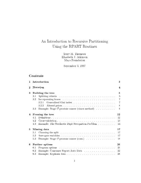
24 patients revived / 144 not revived
H
HHHHHHHH
X 1 =1
22 / 13
H HHHH
X 1 =2, 3 or 4
2 / 131
H HHHH
X 2 =1
20/5
X 2 =2 or 3
2/8
X 3 =1
2/31
X 3 =2 or 3
0 / 100
Figure 1: Revival data
1 Introduction
This document is an update of a technical report written several years ago at Stanford
[5], and is intended to give a short overview of the methods found in the rpart
routines, which implement many of the ideas found in the CART (Classication and
Regression Trees) book and programs of Breiman, Friedman, Olshen and Stone [1].
Because CART is the trademarked name of a particular software implementation of
these ideas, and tree has been used for the S-plus routines of Clark and Pregibon[2]
a dierent acronym | Recursive PARTitioning or rpart | was chosen.
The rpart programs build classication or regression models of a very general
structure using a two stage procedure; the resulting models can be represented as
binary trees. An example is some preliminary data gathered at Stanford on revival
of cardiac arrest patients by paramedics. The goal is to predict which patients
are revivable in the eld on the basis of fourteen variables known at or near the
time of paramedic arrival, e.g., sex, age, time from arrest to rst care, etc. Since
some patients who are not revived on site are later successfully resuscitated at the
hospital, early identication of these \recalcitrant" cases is of considerable clinical
interest.
The resultant model separated the patients into four groups as shown in gure
1, where
X 1 = initial heart rhythm
1= VF/VT, 2=EMD, 3=Asystole, 4=Other
X 2 = initial response to debrillation
3

1=Improved, 2=No change, 3=Worse
X 3 = initial response to drugs
1=Improved, 2=No change, 3=Worse
The other 11 variables did not appear in the nal model. This procedure seems
to work especially well for variables such asX 1 , where there is a denite ordering,
but spacings are not necessarily equal.
The tree is built by the following process: rst the single variable is found which
best splits the data into two groups (`best' will be dened later). The data is
separated, and then this process is applied separately to each sub-group, and so on
recursively until the subgroups either reach a minimum size (5 for this data) or until
no improvement can be made.
The resultant model is, with certainty, too complex, and the question arises as it
does with all stepwise procedures of when to stop. The second stage of the procedure
consists of using cross-validation to trim back the full tree. In the medical example
above the full tree had ten terminal regions. A cross validated estimate of risk was
computed for a nested set of subtrees; this nal model, presented in gure 1, is the
subtree with the lowest estimate of risk.
2 Notation
The partitioning method can be applied to many dierent kinds of data. We will
start by looking at the classication problem, which isoneof the more instructive
cases (but also has the most complex equations). The sample population consists
of n observations from C classes. A given model will break these observations into
k terminal groups; to each of these groups is assigned a predicted class (this will be
the response variable). In an actual application, most parameters will be estimated
from the data, such estimates are given by formulae.
i i =1; 2; :::; C Prior probabilities of each class.
L(i; j) i =1; 2; :::; C Loss matrix for incorrectly classifying
an i as a j. L(i; i) 0:
A
Some node of the tree.
Note that A represents both a set of individuals in
the sample data, and, via the tree that produced it,
a classication rule for future data.
4

(x)
(A)
True class of an observation x, where x is the
vector of predictor variables.
The class assigned to A, if A were to be taken as a
nal node.
n i ;n A Number of observations in the sample that are class i,
number of obs in node A.
n iA Number of observations in the sample that are class i and node A.
P (A)
p(ijA)
R(A)
R(T )
Probability ofA (for future observations).
= P C
i=1
i P fx 2 A j (x) =ig
P C
i=1
i n iA =n i )
P f(x) =i j x 2 Ag (for future observations)
= i P fx 2 A j (x) =ig=P fx 2 Ag
i (n iA =n i )= P i (n iA =n i
Risk of A
= P C
i=1
p(ijA)L(i; (A))
where (A) ischosen to minimize this risk.
Risk of a model (or tree) T
= P k
j=1
P (A j )R(A j )
where A j are the terminal nodes of the tree.
If L(i; j) = 1 for all i 6= j, and we set the prior probabilities equal to the
observed class frequencies in the sample then p(ijA) = n iA =n A and R(T ) is the
proportion misclassied.
3 Building the tree
3.1 Splitting criteria
If we split a node A into two sons A L and A R (left and right sons), we will have
P (A L )R(A L )+P (A R )R(A R ) P (A)R(A)
5

(this is proven in [1]). Using this, one obvious way to build a tree is to choose
that split which maximizes R, the decrease in risk. There are defects with this,
however, as the following example shows.
Suppose losses are equal and that the data is 80% class 1's, and that
some trial split results in A L being 54% class 1's and A R being 100%
class 1's. Class 1's versus class 0's are the outcome variable in this
example. Since the minimum risk prediction for both the left and right
son is (A L )=(A R ) = 1, this split will have R =0,yet scientically
this is a very informative division of the sample. In real data with such
a majority, the rst few splits very often can do no better than this.
A more serious defect with maximizing R is that the risk reduction is essentially
linear. If there were two competing splits, one separating the data into groups of
85% and 50% purity respectively, and the other into 70%-70%, we would usually
prefer the former, if for no other reason than because it better sets things up for the
next splits.
One way around both of these problems is to use lookahead rules; but these
are computationally very expensive. Instead rpart uses one of several measures of
impurity, or diversity, of a node. Let f be some impurity function and dene the
impurity ofanodeAas
I(A) =
CX
i=1
f(p iA )
where p iA is the proportion of those in A that belong to class i for future samples.
Since we would like I(A) =0 when A is pure, f must be concave with f(0) = f(1) =
0.
Two candidates for f are the information index f(p) =,p log(p) and the Gini
index f(p) =p(1 , p). We then use that split with maximal impurity reduction
I = p(A)I(A) , p(A L )I(A L ) , p(A R )I(A R )
The two impurity functions are plotted in gure (2), with the second plot scaled
so that the maximum for both measures is at 1. For the two class problem the
measures dier only slightly, and will nearly always choose the same split point.
Another convex criteria not quite of the above class is twoing for which
I(A) =min
C 1 C 2
[f(p C1 )+f(p C2 )]
where C 1 ,C 2 is some partition of the C classes into two disjoint sets. If C =2twoing
is equivalent to the usual impurity index for f. Surprisingly,twoing can be calculated
almost as eciently as the usual impurity index. One potential advantage of twoing
6

Impurity
0.0 0.2 0.4 0.6
Gini criteria
Information
Scaled Impurity
0.0 0.2 0.4 0.6 0.8 1.0
Gini criteria
Information
0.0 0.2 0.4 0.6 0.8 1.0
0.0 0.2 0.4 0.6 0.8 1.0
P
P
Figure 2: Comparison of Gini and Information indices
is that the output may give the user additional insight concerning the structure of
the data. It can be viewed as the partition of C into two superclasses which are in
some sense the most dissimilar for those observations in A. For certain problems
there may be a natural ordering of the response categories (e.g. level of education),
in which case ordered twoing can be naturally dened, by restricting C 1 to be an
interval [1; 2;:::;k] of classes. Twoing is not part of rpart.
3.2 Incorporating losses
One salutatory aspect of the risk reduction criteria not found in the impurity measures
is inclusion of the loss function. Two dierent ways of extending the impurity
criteria to also include losses are implemented in CART, the generalized Gini index
and altered priors. The rpart software implements only the altered priors method.
3.2.1 Generalized Gini index
The Gini index has the following interesting interpretation. Suppose an object is
selected at random from one of C classes according to the probabilities (p 1 ;p 2 ; :::; p C )
and is randomly assigned to a class using the same distribution. The probability of
7

misclassication is
XX
i
j6=i
p i p j = X i
X
j
p i p j , X i
p 2 i = X i
1 , p 2 i
= Gini index for p
Let L(i; j) be the loss of assigning class j to an object which actually belongs to class
i. The expected cost of misclassication is PP L(i; j)p i p j . This suggests dening
a generalized Gini index of impurity by
G(p) = X i
X
j
L(i; j)p i p j
The corresponding splitting criterion appears to be promising for applications
involving variable misclassication costs. But there are several reasonable objections
to it. First, G(p) is not necessarily a concave function of p, whichwas the motivating
factor behind impurity measures. More seriously, G symmetrizes the loss matrix
before using it. To see this note that
G(p) =(1=2) XX [L(i; j)+L(j; i)] p i p j
In particular, for two-class problems, G in eect ignores the loss matrix.
3.2.2 Altered priors
Remember the denition of R(A)
R(A)
=
CX
i=1
CX
i=1
p iA L(i; (A))
Assume there exists ~ and ~ L be such that
i L(i; (A))(n iA =n i )(n=n A )
~ i
~ L(i; j) =i L(i; j) 8i; j 2 C
Then R(A) is unchanged under the new losses and priors. If L ~ is proportional to
the zero-one loss matrix then the priors ~ should be used in the splitting criteria.
This is possible only if L is of the form
(
Li i 6= j
L(i; j) =
0 i = j
8

in which case
~ i = iL
P i
j jL j
This is always possible when C =2,and hence altered priors are exact for the two
class problem. For P arbitrary loss matrix of dimension C > 2, rpart uses the above
formula with L i = j L(i; j).
A second justication for altered priors is this. An impurity index I(A) =
P f(pi ) has its maximum at p 1 = p 2 = ::: = p C = 1=C. If a problem had, for
instance, a misclassication loss for class 1 which was twice the loss for a class 2 or
3 observation, one would wish I(A) to have its maximum at p 1 =1/5, p 2 = p 3 =2/5,
since this is the worst possible set of proportions on which to decide a node's class.
The altered priors technique does exactly this, by shifting the p i .
Two nal notes
When altered priors are used, they aect only the choice of split. The ordinary
losses and priors are used to compute the risk of the node. The altered priors
simply help the impurity rule choose splits that are likely to be \good" in
terms of the risk.
The argument for altered priors is valid for both the gini and information
splitting rules.
3.3 Example: Stage C prostate cancer (class method)
This rst example is based on a data set of 146 stage C prostate cancer patients
[4]. The main clinical endpoint ofinterest is whether the disease recurs after initial
surgical removal of the prostate, and the time interval to that progression (if any).
The endpoint in this example is status, which takes on the value 1 if the disease has
progressed and 0 if not. Later we'll analyze the data using the exponential (exp)
method, which will take into account time to progression. A short description of
each of the variables is listed below. The main predictor variable of interest in this
study was DNA ploidy, as determined by ow cytometry. For diploid and tetraploid
tumors, the ow cytometric method was also able to estimate the percent of tumor
cells in a G 2 (growth) stage of their cell cycle; G 2 % is systematically missing for
most aneuploid tumors.
The variables in the data set are
9

grade11.845
g262.5
Prog
Prog
Figure 3: Classication tree for the Stage C data
pgtime time to progression, or last follow-up free of progression
pgstat status at last follow-up (1=progressed, 0=censored)
age age at diagnosis
eet early endocrine therapy (1=no, 0=yes)
ploidy diploid/tetraploid/aneuploid DNA pattern
g2 % of cells in G 2 phase
grade tumor grade (1-4)
gleason Gleason grade (3-10)
The model is t by using the rpart function. The rst argument of the function
is a model formula, with the symbol standing for \is modeled as". The print
function gives an abbreviated output, as for other S models. The plot and text
command plot the tree and then label the plot, the result is shown in gure 3.
> progstat cfit print(cfit)
node), split, n, loss, yval, (yprob)
* denotes terminal node
1) root 146 54 No ( 0.6301 0.3699 )
10

2) grade2.5 85 40 Prog ( 0.4706 0.5294 )
6) g211.845 7 1 No ( 0.8571 0.1429 ) *
25) g213.2 45 17 Prog ( 0.3778 0.6222 )
14) g2>17.91 22 8 No ( 0.6364 0.3636 )
28) age>62.5 15 4 No ( 0.7333 0.2667 ) *
29) age text(cfit)
The creation of a labeled factor variable as the response improves the labeling
of the printout.
We have explicitly directed the routine to treat progstat as a categorical variable
by asking for method='class'. (Since progstat is a factor this would have
been the default choice). Since no optional classication parameters are specied
the routine will use the Gini rule for splitting, prior probabilities that are
proportional to the observed data frequencies, and 0/1 losses.
The child nodes of node x are always numbered 2x (left) and 2x +1 (right),
to help in navigating the printout (compare the printout to gure 3).
Other items in the list are the denition of the variable and split used to create
a node, the number of subjects at the node, the loss or error at the node (for
this example, with proportional priors and unit losses this will be the number
misclassied), the classication of the node, and the predicted class for the
node.
* indicates that the node is terminal.
Grades 1 and 2 go to the left, grades 3 and 4 go to the right. The tree is
arranged so that the branches with the largest \average class" go to the right.
11

4 Pruning the tree
4.1 Denitions
We have built a complete tree, possibly quite large and/or complex, and must now
decide how much of that model to retain. In forward stepwise regression, for instance,
this issue is addressed sequentially and no additional variables are added
when the F-test for the remaining variables fails to achieve some level .
Let T 1 , T 2 ,....,T k be the terminal nodes of a tree T. Dene
jT j =number of terminal nodes
risk of T = R(T )= P k
i=1
P (T i )R(T i )
In comparison to regression, jT j is analogous to the model degrees of freedom and
R(T ) to the residual sum of squares.
Now let be some number between 0 and 1 which measures the 'cost' of adding
another variable to the model; will be called a complexity parameter. Let R(T 0 )
be the risk for the zero split tree. Dene
R (T )=R(T )+jT j
to be the cost for the tree, and dene T to be that subtree of the full model which
has minimal cost. Obviously T 0 = the full model and T1 = the model with no splits
at all. The following results are shown in [1].
1. If T 1 and T 2 are subtrees of T with R (T 1 ) = R (T 2 ), then either T 1 is a
subtree of T 2 or T 2 is a subtree of T 1 ; hence either jT 1 j < jT 2 j or jT 2 j < jT 1 j.
2. If >then either T = T or T is a strict subtree of T .
3. Given some set of numbers 1 ; 2 ;:::; m ; both T 1 ;:::;T m and R(T 1 ), :::,
R(T m ) can be computed eciently.
Using the rst result, we can uniquely dene T as the smallest tree T for which
R (T ) is minimized.
Since any sequence of nested trees based on T has at most jT j members, result
2 implies that all possible values of can be grouped into m intervals, m jT j
I 1 = [0; 1 ]
I 2 = ( 1 ; 2 ]
.
I m = ( m,1; 1]
where all 2 I i share the same minimizing subtree.
12

4.2 Cross-validation
Cross-validation is used to choose a best value for by the following steps:
1. Fit the full model on the data set
compute I 1 ;I 2 ; :::; I m
set 1 =0
2 = p 1 2
3 = p 2 3
.
m,1 = p m,2 m,1
m = 1
each i is a `typical value' for its I i
2. Divide the data set into s groups G 1 ;G 2 ; :::; G s each of size s=n, and for each
group separately:
t a full model on the data set `everyone except G i ' and determine
T 1 ;T 2 ; :::; T m for this reduced data set,
compute the predicted class for each observation in G i , under each ofthe
models T j for 1 j m,
from this compute the risk for each subject.
3. Sum over the G i to get an estimate of risk for each j . For that (complexity
parameter) with smallest risk compute T for the full data set, this is chosen
as the best trimmed tree.
In actual practice, we may use instead the 1-SE rule. A plot of versus risk often
has an initial sharp drop followed by arelatively at plateau and then a slow rise.
The choice of among those models on the plateau can be essentially random. To
avoid this, both an estimate of the risk and its standard error are computed during
the cross-validation. Any risk within one standard error of the achieved minimum
is marked as being equivalent to the minimum (i.e. considered to be part of the
at plateau). Then the simplest model, among all those \tied" on the plateau, is
chosen.
In the usual denition of cross-validation we would have taken s = n above, i.e.,
each of the G i would contain exactly one observation, but for moderate n this is
computationally prohibitive. Avalue of s = 10 has been found to be sucient, but
users can vary this if they wish.
In Monte-Carlo trials, this method of pruning has proven very reliable for screening
out `pure noise' variables in the data set.
13

4.3 Example: The Stochastic Digit Recognition Problem
This example is found in section 2.6 of [1], and used as a running example throughout
much of their book. Consider the segments of an unreliable digital readout
1
2 3
4
5
6
7
where each light is correct with probability 0.9, e.g., if the true digit is a 2, the lights
1, 3, 4, 5, and 7 are on with probability 0.9 and lights 2 and 6 are on with probability
0.1. Construct test data where Y 2f0; 1; :::; 9g, each with proportion 1/10 and
the X i , i =1;:::;7 are i.i.d. Bernoulli variables with parameter depending on Y.
X 8 ,X 24 are generated as i.i.d bernoulli P fX i =1g = :5, and are independent ofY.
They correspond to imbedding the readout in a larger rectangle of random lights.
A sample of size 200 was generated accordingly and the procedure applied using
the gini index (see 3.2.1) to build the tree. The S-plus code to compute the simulated
data and the t are shown below.
> n temp lights temp1 temp1 temp2 x

x.7>0.5
|
x.3>0.5
x.4

5 0.0555556 8 0.36111 0.56111 0.0392817
6 0.0166667 9 0.30556 0.36111 0.0367990
7 0.0111111 11 0.27222 0.37778 0.0372181
8 0.0083333 12 0.26111 0.36111 0.0367990
9 0.0055556 16 0.22778 0.35556 0.0366498
10 0.0027778 27 0.16667 0.34444 0.0363369
11 0.0013889 31 0.15556 0.36667 0.0369434
12 0.0000000 35 0.15000 0.36667 0.0369434
> fit9 plot(fit9, branch=.3, compress=T)
> text(fit9)
The cp table diers from that in section 3.5 of [1] in several ways, the last two
of which are somewhat important.
The actual values are dierent, of course, because of dierent random number
generators in the two runs.
The table is printed from the smallest tree (no splits) to the largest one (35
splits). We nd it easier to compare one tree to another when they start at
the same place.
The number of splits is listed, rather than the number of nodes. The number
of nodes is always 1 + the number of splits.
For easier reading, the error columns have been scaled so that the rst node
has an error of 1. Since in this example the model with no splits must make
180/200 misclassications, multiply columns 3-5 by 180 to get a result in
terms of absolute error. (Computations are done on the absolute error scale,
and printed on relative scale).
The complexity parameter column (cp) has been similarly scaled.
Looking at the cp table, we see that the best tree has 10 terminal nodes (9 splits),
based on cross-validation (using 1-SE rule of 0:3444 + 0:0363369). This subtree is
extracted with call to prune and saved in fit9. The pruned tree is shown in gure
4. Two options have been used in the plot. The compress option tries to narrow the
printout by vertically overlapping portions of the plot. (It has only a small eect on
this particular dendrogram). The branch option controls the shape of the branches
that connect a node to its children. The section on plotting (9) will discuss this and
other options in more detail.
The largest tree, with 36 terminal nodes, correctly classies 170/200 = 85%
(1 , 0:15) of the observations, but uses several of the random predictors in doing
16

so and seriously overts the data. If the number of observations per terminal node
(minbucket) had been set to 1 instead of 2, then every observation would be classied
correctly in the nal model, many in terminal nodes of size 1.
5 Missing data
5.1 Choosing the split
Missing values are one of the curses of statistical models and analysis. Most procedures
deal with them by refusing to deal with them { incomplete observations are
tossed out. Rpart is somewhat more ambitious. Any observation with values for
the dependent variable and at least one independent variable will participate in the
modeling.
The quantity to be maximized is still
I = p(A)I(A) , p(A L )I(A L ) , p(A R )I(A R )
The leading term is the same for all variables and splits irrespective of missing
data, but the right two terms are somewhat modied. Firstly, the impurity indices
I(A R ) and I(A L ) are calculated only over the observations which are not missing
a particular predictor. Secondly, the two probabilities p(A L ) and p(A R ) are also
calculated only over the relevant observations, but they are then adjusted so that
they sum to p(A). This entails some extra bookkeeping as the tree is built, but
ensures that the terminal node probabilities sum to 1.
In the extreme case of a variable for which only 2 observations are non-missing,
the impurity of the two sons will both be zero when splitting on that variable. Hence
I will be maximal, and this `almost all missing' coordinate is guaranteed to be
chosen as best; the method is certainly awed in this extreme case. It is dicult to
say whether this bias toward missing coordinates carries through to the non-extreme
cases, however, since a more complete variable also aords for itself more possible
values at which to split.
5.2 Surrogate variables
Once a splitting variable and a split point for it have been decided, what is to
be done with observations missing that variable? One approach is to estimate the
missing datum using the other independent variables; rpart uses a variation of this
to dene surrogate variables.
As an example, assume that the split (age

ecursion) to predict the two categories `age printcp(fit)
Classification tree:
rpart(formula = progstat ~ age + eet + g2 + grade + gleason + ploidy,
data = stagec)
18

Variables actually used in tree construction:
[1] age g2 grade ploidy
Root node error: 54/146 = 0.36986
CP nsplit rel error xerror xstd
1 0.104938 0 1.00000 1.0000 0.10802
2 0.055556 3 0.68519 1.1852 0.11103
3 0.027778 4 0.62963 1.0556 0.10916
4 0.018519 6 0.57407 1.0556 0.10916
5 0.010000 7 0.55556 1.0556 0.10916
> summary(cfit,cp=.06)
Node number 1: 146 observations, complexity param=0.1049
predicted class= No expected loss= 0.3699
class counts: 92 54
probabilities: 0.6301 0.3699
left son=2 (61 obs) right son=3 (85 obs)
Primary splits:
grade < 2.5 to the left, improve=10.360, (0 missing)
gleason < 5.5 to the left, improve= 8.400, (3 missing)
ploidy splits as LRR, improve= 7.657, (0 missing)
g2 < 13.2 to the left, improve= 7.187, (7 missing)
age < 58.5 to the right, improve= 1.388, (0 missing)
Surrogate splits:
gleason < 5.5 to the left, agree=0.8630, (0 split)
ploidy splits as LRR, agree=0.6438, (0 split)
g2 < 9.945 to the left, agree=0.6301, (0 split)
age < 66.5 to the right, agree=0.5890, (0 split)
Node number 2: 61 observations
predicted class= No expected loss= 0.1475
class counts: 52 9
probabilities: 0.8525 0.1475
Node number 3: 85 observations, complexity param=0.1049
predicted class= Prog expected loss= 0.4706
class counts: 40 45
probabilities: 0.4706 0.5294
left son=6 (40 obs) right son=7 (45 obs)
Primary splits:
g2 < 13.2 to the left, improve=2.1780, (6 missing)
ploidy splits as LRR, improve=1.9830, (0 missing)
age < 56.5 to the right, improve=1.6600, (0 missing)
19

gleason < 8.5 to the left, improve=1.6390, (0 missing)
eet < 1.5 to the right, improve=0.1086, (1 missing)
Surrogate splits:
ploidy splits as LRL, agree=0.9620, (6 split)
age < 68.5 to the right, agree=0.6076, (0 split)
gleason < 6.5 to the left, agree=0.5823, (0 split)
.
.
.
There are 54 progressions (class 1) and 92 non-progressions, so the rst node
has an expected loss of 54=146 0:37. (The computation is this simple only
for the default priors and losses).
Grades 1 and 2 go to the left, grades 3 and 4 to the right. The tree is arranged
so that the \more severe" nodes go to the right.
The improvement is n times the change in impurity index. In this instance,
the largest improvement is for the variable grade, with an improvement of
10.36. The next best choice is Gleason score, with an improvement of 8.4.
The actual values of the improvement are not so important, but their relative
size gives an indication of the comparitive utility of the variables.
Ploidy is a categorical variable, with values of diploid, tetraploid, and aneuploid,
in that order. (To check the order, type table(stagec$ploidy)). All
three possible splits were attempted: anueploid+diploid vs. tetraploid, anueploid+tetraploid
vs. diploid, and anueploid vs. diploid + tetraploid. The best
split sends diploid to the right and the others to the left (node 6, see gure
(3).
For node 3, the primary split variable is missing on 6 subjects. All 6 are split
based on the rst surrogate, ploidy. Diploid and aneuploid tumors are sent to
the left, tetraploid to the right.
6 Further options
6.1 Program options
g2 < 13.2 g2 > 13.2 NA
Diploid/aneuploid 33 2 5
Tetraploid 1 43 1
The central tting function is rpart, whose main arguments are
20

formula: the model formula, as in lm and other S model tting functions. The
right hand side may contain both continuous and categorical (factor) terms.
If the outcome y has more than two levels, then categorical predictors must
be t by exhaustive enumeration, which can take avery long time.
data, weights, subset: as for other S models. Weights are not yet supported,
and will be ignored if present.
method: the type of splitting rule to use. Options at this point are classication,
anova, Poisson, and exponential.
parms: a list of method specic optional parameters. For classication, the list
can contain any of: the vector of prior probabilities (component prior), the
loss matrix (component loss) or the splitting index (component split). The
priors must be positive and sum to 1. The loss matrix must have zeros on the
diagonal and positive o-diagonal elements. The splitting index can be `gini'
or `information'.
na.action: the action for missing values. The default action for rpart is
na.rpart, this default is not overridden by the options(na.action) global option.
The default action removes only those rows for which either the response
y or all of the predictors are missing. This ability toretain partially missing
observations is perhaps the single most useful feature of rpart models.
control: a list of control parameters, usually the result of the rpart.control
function. The list must contain
{ minsplit: The minimum number of observations in a node for which
the routine will even try to compute a split. The default is 20. This
parameter can save computation time, since smaller nodes are almost
always pruned away by cross-validation.
{ minbucket: The minimum number of observations in a terminal node.
This defaults to minsplit/3.
{ maxcompete: It is often useful in the printout to see not only the variable
that gave the best split at a node, but also the second, third, etc best.
This parameter controls the number that will be printed. It has no eect
on computational time, and a small eect on the amount of memory used.
The default is 5.
{ xval: The number of cross-validations to be done. Usually set to zero
during exploritory phases of the analysis. A value of 10, for instance,
increases the compute time to 11-fold overavalue of 0.
21

{ maxsurrogate: The maximum number of surrogate variables to retain at
each node. (No surrogate that does worse than \go with the majority"
is printed or used). Setting this to zero will cut the computation time
in half, and set usesurrogate to zero. The default is 5. Surrogates give
dierent information than competitor splits. The competitor list asks
\which other splits would have as many correct classications", surrogates
ask \which other splits would classify the same subjects in the
same way", which is a harsher criteria.
{ usesurrogate: A value of usesurrogate=2, the default, splits subjects in
the way described previously. This is similar to CART. If the value is 0,
then a subject who is missing the primary split variable does not progress
further down the tree. Avalue of 1 is intermediate: all surrogate variables
except \go with the majority" are used to send a case further down the
tree.
{ cp: The threshold complexity parameter.
The complexity parameter cp is, like minsplit, an advisory parameter, but is
considerably more useful. It is specied according to the formula
R cp (T ) R(T )+cp jT jR(T 0 )
where T 0 is the tree with no splits. This scaled version is much more user friendly
than the original CART formula (4.1) since it is unitless. Avalue of cp=1 will always
result in a tree with no splits. For regression models (see next section) the scaled cp
hasavery direct interpretation: if any split does not increase the overall R 2 of the
model by at least cp (where R 2 is the usual linear-models denition) then that split is
decreed to be, a priori, not worth pursuing. The program does not split said branch
any further, and saves considerable computational eort. The default value of .01
has been reasonably successful at `pre-pruning' trees so that the cross-validation
step need only remove 1 or 2 layers, but it sometimes overprunes, particularly for
large data sets.
6.2 Example: Consumer Report Auto Data
A second example using the class method demonstrates the outcome for a response
with multiple (> 2) categories. We also explore the dierence between Gini and information
splitting rules. The dataset cu.summary contains a collection of variables
from the April, 1990 Consumer Reports summary on 117 cars. For our purposes,
22

Country:dghij
|
Country:dghij
|
Much worse
(7/0/2/0/0)
Type:e
average
(7/4/16/0/0)
Type:bcf
Country:gj
worse
(4/6/1/3/0)
average
(0/2/4/2/0)
Much bette
(0/0/3/3/21)
Type:e
Type:bcef
Much worse average
(7/0/2/0/0) (7/4/16/0/0)
Country:gj
worse average
(4/6/1/3/0) (0/2/4/2/0)
Much bette
(0/0/3/3/21)
Figure 5: Displays the rpart-based model relating automobile Reliability to car type,
price, and country of origin. The gure on the left uses the gini splitting index and
the gure on the right uses the information splitting index.
car reliability will be treated as the response. The variables are:
Reliabilty
Price
Country
Mileage
Type
an ordered factor (contains NAs):
Much worse < worse < average < better < Much Better
numeric: list price in dollars, with standard equipment
factor: country where car manufactured
(Brazil, England, France, Germany, Japan,
Japan/USA, Korea, Mexico, Sweden, USA)
numeric: gas mileage in miles/gallon, contains NAs
factor: Small, Sporty, Compact, Medium, Large, Van
In the analysis we are treating reliability asan unordered outcome. Nodes potentially
can be classied as much worse, worse, average, better, or much better, though
there are none that are labelled as just \better". The 32 cars with missing response
(listed as NA) were not used in the analysis. Two ts are made, one using the Gini
index and the other the information index.
> fit1 fit2

data=cu.summary, parms=list(split='information'))
> par(mfrow=c(1,2))
> plot(fit1); text(fit1,use.n=T,cex=.9)
> plot(fit2); text(fit2,use.n=T,cex=.9)
The rst two nodes from the Gini tree are
Node number 1: 85 observations, complexity param=0.3051
predicted class= average expected loss= 0.6941
class counts: 18 12 26 8 21
probabilities: 0.2118 0.1412 0.3059 0.0941 0.2471
left son=2 (58 obs) right son=3 (27 obs)
Primary splits:
Country splits as ---LRRLLLL, improve=15.220, (0 missing)
Type splits as RLLRLL, improve= 4.288, (0 missing)
Price < 11970 to the right, improve= 3.200, (0 missing)
Mileage < 24.5 to the left, improve= 2.476, (36 missing)
Node number 2: 58 observations, complexity param=0.08475
predicted class= average expected loss= 0.6034
class counts: 18 12 23 5 0
probabilities: 0.3103 0.2069 0.3966 0.0862 0.0000
left son=4 (9 obs) right son=5 (49 obs)
Primary splits:
Type splits as RRRRLR, improve=3.187, (0 missing)
Price < 11230 to the left, improve=2.564, (0 missing)
Mileage < 24.5 to the left, improve=1.802, (30 missing)
Country splits as ---L--RLRL, improve=1.329, (0 missing)
The t for the information splitting rule is
Node number 1: 85 observations, complexity param=0.3051
predicted class= average expected loss= 0.6941
class counts: 18 12 26 8 21
probabilities: 0.2118 0.1412 0.3059 0.0941 0.2471
left son=2 (58 obs) right son=3 (27 obs)
Primary splits:
Country splits as ---LRRLLLL, improve=38.540, (0 missing)
Type splits as RLLRLL, improve=11.330, (0 missing)
Price < 11970 to the right, improve= 6.241, (0 missing)
Mileage < 24.5 to the left, improve= 5.548, (36 missing)
Node number 2: 58 observations, complexity param=0.0678
predicted class= average expected loss= 0.6034
class counts: 18 12 23 5 0
24

probabilities: 0.3103 0.2069 0.3966 0.0862 0.0000
left son=4 (36 obs) right son=5 (22 obs)
Primary splits:
Type splits as RLLRLL, improve=9.281, (0 missing)
Price < 11230 to the left, improve=5.609, (0 missing)
Mileage < 24.5 to the left, improve=5.594, (30 missing)
Country splits as ---L--RRRL, improve=2.891, (0 missing)
Surrogate splits:
Price < 10970 to the right, agree=0.8793, (0 split)
Country splits as ---R--RRRL, agree=0.7931, (0 split)
The rst 3 countries (Brazil, England, France) had only one or two cars in
the listing, all of which were missing the reliability variable. There are no entries
for these countries in the rst node, leading to the , symbol for the rule. The
information measure has larger \improvements", consistent with the dierence in
scaling between the information and Gini criteria shown in gure 2, but the relative
merits of dierent splits are fairly stable.
The two rules do not choose the same primary split at node 2. The data at this
point are
Compact Large Medium Small Sporty Van
Much worse 2 2 4 2 7 1
worse 5 0 4 3 0 0
average 3 5 8 2 2 3
better 2 0 0 3 0 0
Much better 0 0 0 0 0 0
Since there are 6 dierent categories, all 2 5 = 32 dierent combinations were explored,
and as it turns out there are several with a nearly identical improvement.
The Gini and information criteria make dierent \random" choices from this set
of near ties. For the Gini index, Sporty vs others Compact/Small vs others have
improvements of 37.19 and 37.20, respectively. For the information index, the improvements
are 67.3 versus 64.2, respectively. Interestingly, the two splitting criteria
arrive at exactly the same nal nodes, for the full tree, although by dierent paths.
(Compare the class counts of the terminal nodes).
We have said that for a categorical predictor with m levels, all 2 m,1 dierent
possible splits are tested.. When there are a large number of categories for the
predictor, the computational burden of evaluating all of these subsets can become
large. For instance, the call rpart(Reliabilty ., data=car.all) does not return
for a long, long time: one of the predictors in that data set is a factor with 79 levels!
Luckily, for any ordered outcome there is a computational shortcut that allows the
program to nd the best split using only m , 1 comparisons. This includes the
25

|
Start>8.5
absent
(64/17)
Start>12.5 |
absent
(64/17)
Start>8.5 |
absent
(64/17)
Start>14.5
absent
(56/6) Age111
absent absent
(12/0) (15/6)
present
(8/11)
absent
(44/2)
Age lmat fit1 fit2

parms=list(prior=c(.65,.35)))
> fit3 par(mfrow=c(1,3))
> plot(fit1); text(fit1,use.n=T,all=T)
> plot(fit2); text(fit2,use.n=T,all=T)
> plot(fit3); text(fit3,use.n=T,all=T)
This example shows how even the initial split changes depending on the prior
and loss that are specied. The rst and third ts have the same initial split (Start
< 8:5), but the improvement diers. The second t splits Start at 12.5 which moves
46 people to the left instead of 62.
Looking at the leftmost tree, we see that the sequence of splits on the left hand
branch yeilds only a single node classied as present. For any loss greater than 4
to 3, the routine will instead classify this node as absent, and the entire left side of
the tree collapses, as seen in the right hand gure. This is not unusual | the most
common eect of alternate loss matrices is to change the amount of pruning in the
tree, more in some branches and less in others, rather than to change the choice of
splits.
The rst node from the default tree is
Node number 1: 81 observations, complexity param=0.1765
predicted class= absent expected loss= 0.2099
class counts: 64 17
probabilities: 0.7901 0.2099
left son=2 (62 obs) right son=3 (19 obs)
Primary splits:
Start < 8.5 to the right, improve=6.762, (0 missing)
Number < 5.5 to the left, improve=2.867, (0 missing)
Age < 39.5 to the left, improve=2.250, (0 missing)
Surrogate splits:
Number < 6.5 to the left, agree=0.8025, (0 split)
The t using the prior (0.65,0.35) is
Node number 1: 81 observations, complexity param=0.302
predicted class= absent expected loss= 0.35
class counts: 64 17
probabilities: 0.65 0.35
left son=2 (46 obs) right son=3 (35 obs)
Primary splits:
Start < 12.5 to the right, improve=10.900, (0 missing)
27

Number < 4.5 to the left, improve= 5.087, (0 missing)
Age < 39.5 to the left, improve= 4.635, (0 missing)
Surrogate splits:
Number < 3.5 to the left, agree=0.6667, (0 split)
And rst split under 4/3 losses is
Node number 1: 81 observations, complexity param=0.01961
predicted class= absent expected loss= 0.6296
class counts: 64 17
probabilities: 0.7901 0.2099
left son=2 (62 obs) right son=3 (19 obs)
Primary splits:
Start < 8.5 to the right, improve=5.077, (0 missing)
Number < 5.5 to the left, improve=2.165, (0 missing)
Age < 39.5 to the left, improve=1.535, (0 missing)
Surrogate splits:
Number < 6.5 to the left, agree=0.8025, (0 split)
7 Regression
7.1 Denition
Up to this point the classication problem has been used to dene and motivate our
formulae. However, the partitioning procedure is quite general and can be extended
by specifying 5 \ingredients":
A splitting criterion, which is used to decide which variable gives the best
split. For classication this was either the Gini or log-likelihood function. In
the anova method the splitting criteria is SS T , (SS L + SS R ), where SS T =
P (yi , y) 2 is the sum of squares for the node, and SS R , SS L are the sums of
squares for the right and left son, respectively. This is equivalent to chosing
the split to maximize the between-groups sum-of-squares in a simple analysis
of variance. This rule is identical to the regression option for tree.
A summary statistic or vector, which is used to describe a node. The rst
element of the vector is considered to be the tted value. For the anova
method this is the mean of the node; for classication the response is the
predicted class followed by the vector of class probabilities.
The error of a node. This will be the variance of y for anova, and the predicted
loss for classication.
28

The prediction error for a new observation, assigned to the node. For anova
this is (y new , y).
Any necessary initialization.
The anova method leads to regression trees; it is the default method if y a simple
numeric vector, i.e., not a factor, matrix, or survival object.
7.2 Example: Consumer Report Auto data (cont.)
The dataset car.all contains a collection of variables from the April, 1990 Consumer
Reports; it has 36 variables on 111 cars. Documentation may be found in the S-Plus
manual. We will work with a subset of 23 of the variables, created by the rst two
lines of the example below. We will use Price as the response. This data set is
a good example of the usefulness of the missing value logic in rpart: most of the
variables are missing on only 3-5 observations, but only 42/111 have a complete
subset.
> cars cars$Eng.Rev fit3 fit3
node), split, n, deviance, yval
* denotes terminal node
1) root 105 7118.00 15.810
2) Disp.156 35 2351.00 23.700
6) HP.revs5550 11 531.60 30.940 *
> printcp(fit3)
Regression tree:
rpart(formula = Price ~ ., data = cars)
Variables actually used in tree construction:
[1] Country Disp. HP.revs Type
29

Root node error: 7.1183e9/105 = 6.7793e7
CP nsplit rel error xerror xstd
1 0.460146 0 1.00000 1.02413 0.16411
2 0.117905 1 0.53985 0.79225 0.11481
3 0.044491 3 0.30961 0.60042 0.10809
4 0.033449 4 0.26511 0.58892 0.10621
5 0.010000 5 0.23166 0.57062 0.11782
Only 4 of 22 predictors were actually used in the t: engine displacement in cubic
inches, country of origin, type of vehicle, and the revolutions for maximum horsepower
(the \red line" on a tachometer).
The relative error is 1 , R 2 , similar to linear regression. The xerror is related
to the PRESS statistic. The rst split appears to improve the t the most.
The last split adds little improvement to the apparent error.
The 1-SE rule would choose a tree with 3 splits.
This is a case where the default cp value of .01 may have overpruned the tree,
since the cross-validated error is not yet at a minimum. A rerun with the
cp threshold at .002 gave a maximum tree size of 8 splits, with a minimun
cross-validated error for the 5 split model.
For any CPvalue between 0.46015 and 0.11791 the best model has one split;
for any CPvalue between 0.11791 and 0.04449 the best model is with 3 splits;
and so on.
The print command also recognizes the cp option, which allows the user to see
which splits are the most important.
> print(fit3,cp=.10)
node), split, n, deviance, yval
* denotes terminal node
1) root 105 7.118e+09 15810
2) Disp.156 35 2.351e+09 23700
6) HP.revs5550 11 5.316e+08 30940 *
30

The rst split on displacement partitions the 105 observations into groups of
70 and 35 (nodes 2 and 3) with mean prices of 11,860 and 23,700. The deviance
(corrected sum-of-squares) at these 2 nodes are 1:49x10 9 and 2:35x10 9 , respectively.
More detailed summarization of the splits is again obtained by using the function
summary.rpart.
> summary(fit3, cp=.10)
Node number 1: 105 observations, complexity param=0.4601
mean=15810 , SS/n=67790000
left son=2 (70 obs) right son=3 (35 obs)
Primary splits:
Disp. < 156 to the left, improve=0.4601, (0 missing)
HP < 154 to the left, improve=0.4549, (0 missing)
Tank < 17.8 to the left, improve=0.4431, (0 missing)
Weight < 2890 to the left, improve=0.3912, (0 missing)
Wheel.base < 104.5 to the left, improve=0.3067, (0 missing)
Surrogate splits:
Weight < 3095 to the left, agree=0.9143, (0 split)
HP < 139 to the left, agree=0.8952, (0 split)
Tank < 17.95 to the left, agree=0.8952, (0 split)
Wheel.base < 105.5 to the left, agree=0.8571, (0 split)
Length < 185.5 to the left, agree=0.8381, (0 split)
Node number 2: 70 observations, complexity param=0.1123
mean=11860 , SS/n=21310000
left son=4 (58 obs) right son=5 (12 obs)
Primary splits:
Country splits as L-RRLLLLRL, improve=0.5361, (0 missing)
Tank < 15.65 to the left, improve=0.3805, (0 missing)
Weight < 2568 to the left, improve=0.3691, (0 missing)
Type splits as R-RLRR, improve=0.3650, (0 missing)
HP < 105.5 to the left, improve=0.3578, (0 missing)
Surrogate splits:
Tank < 17.8 to the left, agree=0.8571, (0 split)
Rear.Seating < 28.75 to the left, agree=0.8429, (0 split)
.
.
.
The improvement listed is the percent change in sums of squares (SS) for this
split, i.e., 1 , (SS right + SS left )=SS parent .
The weight and displacement are very closely related, as shown by the surrogate
split agreement of 91%.
31

Disp.

R-square
0.0 0.2 0.4 0.6 0.8 1.0
•
•
•
Apparent
X Relative
•
• •
•
•
•
X Relative Error
0.4 0.6 0.8 1.0 1.2
•
•
• •
•
0 1 2 3 4 5
Number of Splits
0 1 2 3 4 5
Number of Splits
Figure 8: Both plots were obtained using the function rsq.rpart(fit3). The gure
on the left shows that the rst split oers the most information. The gure on the
right suggests that the tree should be pruned to include only 1 or 2 splits.
> plot(predict(fit3),resid(fit3))
> axis(3,at=fit3$frame$yval[fit3$frame$var==''],
labels=row.names(fit3$frame)[fit3$frame$var==''])
> mtext('leaf number',side=3, line=3)
> abline(h=0)
7.3 Example: Stage C prostate cancer (anova method)
The stage C prostate cancer data of the earlier section can also be t using the
anova method, by treating the status variable as though it were continuous.
> cfit2 printcp(cfit2)
Regression tree:
rpart(formula = pgstat ~ age + eet + g2 + grade + gleason + ploidy, data =
stagec)
Variables actually used in tree construction:
[1] age g2 grade ploidy
33

leaf number
8 9 12 5 13 7
resid(fit3)
-10000 -5000 0 5000 10000
•
• •
•
•
• •
•
•
•
•
• •
•
•
•
•
•
•
•
•
•
•
•
•
•
• •
•
•
•
•
•
•
•
•
•
•
•
•
•
•
•
•
•
•
10000 15000 20000 25000 30000
predict(fit3)
Figure 9: This plot shows the (observed-expected) cost of cars versus the predicted
cost of cars based on the nodes/leaves in which the cars landed. There appears to be
more variability in node 7 than in some of the other leaves.
Root node error: 34.027/146 = 0.23306
CP nsplit rel error xerror xstd
1 0.152195 0 1.00000 1.01527 0.045470
2 0.054395 1 0.84781 0.86670 0.063447
3 0.032487 3 0.73901 0.86524 0.075460
4 0.019932 4 0.70653 0.95702 0.085390
5 0.013027 8 0.63144 1.05606 0.092566
6 0.010000 9 0.61841 1.07727 0.094466
> print(cfit2, cp=.03)
node), split, n, deviance, yval
* denotes terminal node
1) root 146 34.030 0.3699
2) grade2.5 85 21.180 0.5294
6) g2

7) g2>13.2 45 10.580 0.6222
14) g2>17.91 22 5.091 0.3636 *
15) g2

{ etc.
Such data would usually be approached by using Poisson regression; can we nd
a tree based analogue? In adding criteria for rates regression to this ensemble, the
guiding principle was the following: the between groups sum-of-squares is not a very
robust measure, yet tree based regression works very well. So do the simplest thing
possible.
Let c i be the observed event count for observation i, t i be the observation time,
and x ij ;j =1;:::;p be the predictors. The y variable for the program will be a 2
column matrix.
Splitting criterion: The likelihood ratio test for two Poisson groups
D parent ,
D left son + D right son
Summary statistics: The observed event rate and the number of events.
P
^ = #events
total time = P
ci
ti
Error of a node: The within node deviance.
X" !
c i
D = c i log , (c i ,
^t ^t i )
i
Prediction error: The deviance contribution for a new observation, using ^ of
the node as the predicted rate.
8.2 Improving the method
There is a problem with the criterion just proposed, however: cross-validation of a
model often produces an innite value for the deviance. The simplest case where
this occurs is easy to understand. Assume that some terminal node of the tree has
20 subjects, but only 1 of the 20 has experienced any events. The cross-validated
error (deviance) estimate for that node will have one subset | the one where the
subject with an event is left out | which has ^ =0. When we use the prediction
for the 10% of subjects who were set aside, the deviance contribution of the subject
with an event is
:::+ c i log(c i =0) + :::
which is innite since c i > 0. The problem is that when ^ = 0 the occurrence of an
event is innitely improbable, and, using the deviance measure, the corresponding
model is then innitely bad.
36
#

One might expect this phenomenon to be fairly rare, but unfortunately it is not
so. One given of tree-based modeling is that a right-sized model is arrived at by
purposely over-tting the data and then pruning back the branches. A program
that aborts due to a numeric exception during the rst stage is uninformative to
say the least. Of more concern is that this edge eect does not seem to be limited
to the pathologic case detailed above. Any near approach to the boundary value
=0leads to large values of the deviance, and the procedure tends to discourage
any nal node with a small numberofevents.
An ad hoc solution is to use the revised estimate
^ = max
^;
k
P
ti
where k is 1/2 or 1/6. That is, pure nodes are given a partial event. (This is similar
to the starting estimates used in the GLM program for a Poisson regression.) This
is unsatisfying, however, and we propose instead using a shrinkage estimate.
Assume that the true rates j for the leaves of the tree are random values from
a Gamma(; ) distribution. Set to the observed overall event rate P c i = P t i ,
and let the user choose as a prior the coecient of variation k = =. A value of
k = 0 represents extreme pessimism (\the leaf nodes will all give the same result"),
whereas k = 1 represents extreme optimism. The Bayes estimate of the event rate
for a node works out to be
^ k = + P c i
+ P t i
;
where =1=k 2 and = =^.
This estimate is scale invariant, has a simple interpretation, and shrinks least
those nodes with a large amount of information. In practice, a value of k =10does
essentially no shrinkage. For method='poisson', the optional parameters list is the
single number k, with a default value of 1. This corresponds to prior coecient of
variation of 1 for the estimated j . We have not nearly enough experience to decide
if this is a good value. (It does stop the log(0) message though).
Cross-validation does not work very well. The procedure gives very conservative
results, and quite often declares the no-split tree to be the best. This may be another
artifact of the edge eect.
8.3 Example: solder data
The solder data frame, as explained in the Splus help le, is a design object with 900
observations, which are the results of an experiment varying 5 factors relevant to the
wave-soldering procedure for mounting components on printed circuit boards. The
37

esponse variable, skips, is a count of how many solder skips appeared to a visual
inspection. The other variables are listed below:
Opening factor: amount of clearance around the mounting pad (S < M < L)
Solder factor: amount of solder used (Thin < Thick)
Mask factor: Type of solder mask used (5 possible)
PadType factor: Mounting pad used (10 possible)
Panel factor: panel (1, 2 or 3) on board being counted
In this call, the rpart.control options are modied: maxcompete = 2 means that
only 2 other competing splits are listed (default is 4); cp = .05 means that a smaller
tree will be built initially (default is .01). The y variable for Poisson partitioning
may beatwo column matrix containing the observation time in column 1 and the
number of events in column 2, or it may beavector of event counts alone.
fit

Call:
rpart(formula = skips ~ Opening + Solder + Mask + PadType + Panel, data =
solder, method = "poisson", control = rpart.control(cp = 0.05,
maxcompete = 2))
CP nsplit rel error xerror xstd
1 0.3038 0 1.0000 1.0051 0.05248
2 0.1541 1 0.6962 0.7016 0.03299
3 0.1285 2 0.5421 0.5469 0.02544
4 0.0500 3 0.4137 0.4187 0.01962
Node number 1: 900 observations, complexity param=0.3038
events=4977, estimated rate=5.53 , deviance/n=9.765
left son=2 (600 obs) right son=3 (300 obs)
Primary splits:
Opening splits as RLL, improve=2670, (0 missing)
Mask splits as LLRLR, improve=2162, (0 missing)
Solder splits as RL, improve=1168, (0 missing)
Node number 2: 600 observations, complexity param=0.1285
events=1531, estimated rate=2.553 , deviance/n=4.928
left son=4 (420 obs) right son=5 (180 obs)
Primary splits:
Mask splits as LLRLR, improve=1129.0, (0 missing)
Opening splits as -RL, improve= 250.8, (0 missing)
Solder splits as RL, improve= 219.8, (0 missing)
Node number 3: 300 observations, complexity param=0.1541
events=3446, estimated rate=11.48 , deviance/n=10.54
left son=6 (150 obs) right son=7 (150 obs)
Primary splits:
Mask splits as LLRRR, improve=1354.0, (0 missing)
Solder splits as RL, improve= 976.9, (0 missing)
PadType splits as RRRRLRLRLL, improve= 313.2, (0 missing)
Surrogate splits:
Solder splits as RL, agree=0.6, (0 split)
Node number 4: 420 observations
events=433, estimated rate=1.033 , deviance/n=2.082
Node number 5: 180 observations
events=1098, estimated rate=6.099 , deviance/n=5.295
Node number 6: 150 observations
events=680, estimated rate=4.535 , deviance/n=4.351
39

Opening:bc
|
Opening:bc
|
Mask:abd
Mask:ab
2.553
1531/600
Mask:ab
1.033
433/420
6.099
1098/180 4.535
680/150
18.420
2766/150
4.535
680/150
18.420
2766/150
Figure 10: The rst gure shows the solder data, t with the poisson method, using
a cp value of 0.05. The second gure shows the same t, but with a cp value of 0.15.
The function prune.rpart was used to produce the smaller tree.
Node number 7: 150 observations
events=2766, estimated rate=18.42 , deviance/n=7.701
The improvement is Deviance parent , (Deviance left + Deviance right ), which is
the likelihood ratio test for comparing two Poisson samples.
The cross-validated error has been found to be overly pessimistic when describing
how much the error is improved by each split. This is likely an eect
of the boundary eect mentioned earlier, but more research is needed.
The variation xstd is not as useful, given the bias of xerror.
> plot(fit)
> text(fit,use.n=T)
> fit.prune plot(fit.prune)
> text(fit.prune,use.n=T)
40

The use.n=T option species that number of events / total N should be listed
along with the predicted rate (number of events/person-years). The function prune
trims the tree fit to the cp value 0:15. The same tree could have been created by
specifying cp = .15 in the original call to rpart.
8.4 Example: Stage C prostate cancer (survival method)
One special case of the Poisson model is of particular interest for medical consulting
(such as the authors do). Assume that we have survival data, i.e., each subject has
either 0 or 1 event. Further, assume that the time values have been pre-scaled so as
to t an exponential model. That is, stretch the time axis so that a Kaplan-Meier
plot of the data will be a straight line when plotted on the logarithmic scale. An
approximate way to do this is
temp

3) grade>2.5 85 125.10 1.6230
6) age>56.5 75 104.00 1.4320
12) gleason17.915 14 18.72 0.8795 *
51) g27.5 25 34.13 2.0280
26) g2>15.29 10 11.81 1.2140 *
27) g2 text(fit, use.n=T)
Note that the primary split on grade is the same as when status was used as a
dichotomous endpoint, but that the splits thereafter dier.
> summary(fit,cp=.02)
Call:
rpart(formula = Surv(pgtime, pgstat) ~ age + eet + g2 + grade +
gleason + ploidy, data = stagec)
CP nsplit rel error xerror xstd
1 0.12913 0 1.0000 1.0060 0.07389
2 0.04169 1 0.8709 0.8839 0.07584
3 0.02880 2 0.8292 0.9271 0.08196
4 0.01720 3 0.8004 0.9348 0.08326
5 0.01518 4 0.7832 0.9647 0.08259
6 0.01271 5 0.7680 0.9648 0.08258
7 0.01000 8 0.7311 0.9632 0.08480
Node number 1: 146 observations, complexity param=0.1291
events=54, estimated rate=1 , deviance/n=1.338
left son=2 (61 obs) right son=3 (85 obs)
Primary splits:
grade < 2.5 to the left, improve=25.270, (0 missing)
gleason < 5.5 to the left, improve=21.630, (3 missing)
ploidy splits as LRR, improve=14.020, (0 missing)
g2 < 13.2 to the left, improve=12.580, (7 missing)
age < 58.5 to the right, improve= 2.796, (0 missing)
Surrogate splits:
gleason < 5.5 to the left, agree=0.8630, (0 split)
ploidy splits as LRR, agree=0.6438, (0 split)
42

grade

grade

Prob Progression
0.0 0.2 0.4 0.6 0.8 1.0
node 4
node 5
node 6
node 7
0 5 10 15
Time to Progression
Figure 13: Survival plot based on snipped rpart object. The probability of tumor
progression is greatest in node 7, which has patients who are younger and have a
higher initial tumor grade.
Error (dev) = 103.9783
> plot(fit2)
> text(fit2,use.n=T)
For a nal summary of the model, it can be helpful to plot the probability of
survival based on the nal bins in which the subjects landed. To create new variables
based on the rpart groupings, use where. The nodes of fit2 above are shown in the
right hand panel of gure 12: node 4 has 1 event, 33 subjects, grade = 1-2 and g2
< 11.36; node 5 has 8 events, 28 subjects, grade = 1-2 and g2 > 11.36; node 6 has
37 events, 75 subjects, grade = 3-4, age > 56.5; node 7 has 8 events, 10 subjects,
grade = 3-4, age < 56.5. Patients who are younger and have a higher initial grade
tend to have more rapid progression of disease.
> newgrp plot(survfit(Surv(pgtime,pgstat) ~ newgrp, data=stagec),
mark.time=F, lty=1:4)
> title(xlab='Time to Progression',ylab='Prob Progression')
> legend(.2,.2, legend=paste('node',c(4,5,6,7)), lty=1:4)
45

grade11.845
g2

grade11.845
No
(20/11)
Prog
(3/6)
No
(14/8)
Prog
(3/20)
No
(6/1)
g2 text(fit, use.n=T, all=T)
Fancier plots can be created by modifying the branch option, which controls the
shape of branches that connect a node to its children. The default for the plots
is to have square shouldered trees (branch = 1.0). This can be taken to the other
extreme with no shoulders at all (branch=0) as shown in gure 16.
> plot(fit, branch=0)
> text(fit, use.n=T)
These options can be combined with others to create the plot that ts your
particular needs. The default plot may be inecient in it's use of space: the terminal
nodes will always lie at x-coordinates of 1,2,:::. The compress option attempts to
improve this by overlapping some nodes. It has little eect on gure 17, but in
gure 4 it allows the lowest branch to \tuck under" those above. If you want to
play around with the spacing with compress, try using nspace which regulates the
space between a terminal node and a split.
> plot(fit,branch=.4,uniform=T,compress=T)
> text(fit,all=T,use.n=T)
47

grade11.845
g2

Endpoint = progstat
No
|
(92/54)
grade2.5
No
(52/9)
g211.845
(3/6)
No
g213.2
Prog
(17/28)
g2>17.91
No
g2 plot(tree, uniform = T, branch = 0.2, compress = T, margin = 0.1)
> text(tree, all = T, use.n=T, fancy = T)
The fancy option of text creates the ellipses and rectangles, and moves the splitting
rule to the midpoints of the branches. Margin shrinks the plotting region slightly so
that the text boxes don't run over the edge of the plot. The branch option makes
the lines exit the ellipse at a \good" angle. The call post(fit) will create a postcript
le t.ps in the current directory. The additional argument file="" will cause the
plot to appear on the current active device. Note that post.rpart is just our choice
of options to the functions plot.rpart and text.rpart. The reader is encouraged to
try out other possibilities, as these specications may not be the best choice in all
situations.
10 Other functions
A more general approach to cross-validation can be gained using the xpred.rpart
function. Given an rpart t, a vector of k complexity parameters, and the desired
number of cross-validation groups, this function returns an n by k matrix containing
49

the predicted value ^y (,i) for each subject, from the model that was t without that
subject. The cp vector defaults to the geometric mean of the cp sequence for the
pruned tree on the full data set.
> fit fit$cptable
CP nsplit rel error xerror xstd
1 0.07572983 0 1.0000000 1.012323 0.1321533
2 0.02825076 2 0.8485403 1.094811 0.1547652
3 0.01789441 7 0.7219625 1.216495 0.1603581
4 0.01295145 8 0.7040681 1.223120 0.1610315
5 0.01000000 9 0.6911166 1.227213 0.1660616
> temp err sum.err sum.err / (fit$frame)$dev[1]
0.27519053 0.04625392 0.02248401 0.01522362 0.01138044
1.021901 1.038632 1.14714 1.179571 1.174196
The answer from xpred.rpart diers from the model's computation due to different
random number seeds, which causes slightly dierent cross-validation groups.
11 Relation to other programs
11.1 CART
Almost all of the denitions in rpart are equivalent to those used in CART, and the
output should usually be very similar. The printout given by summary.rpart was
also strongly inuenced by some early cart output. Some known dierences are
Surrogate splits: cart uses the percentage agreement between the surrogate
and the primary split, and rpart uses the total number of agreements. When
one of the surrogate variables has missing values this can lead to a dierent
ordering. For instance, assume that the best surrogate based on x 1 has 45/50
= 90% agreement (with 10 missing), and the best based on x 2 has 46/60 (none
missing). Then rpart will pick x 2 . This is only a serious issue when there
are a large number of missing values for one variable, and indeed the change
was motivated by examples where a nearly-100best surrogate due to perfect
concordance with the primary split.
: Computation: Some versions of the cart code have been optimized for very
large data problems, and include such features as subsampling from the larger
nodes. Large data sets can be a problem in S-plus.
50

11.2 Tree
The user interface to rpart is almost identical to that of the tree functions. In
fact, the rpart object was designed to be a simple superset of the tree class, and
to inherit most methods from it (saving a lot of code writing). However, this close
connection had to be abandoned. The rpart object is still very similiar to tree
objects, diering in 3 respects
Addition of a method component. This was the single largest reason for divergence.
In tree, splitting of a categorical variable results in a yprob element
in the data structure, but regression does not. Most of the \downstream"
functions then contain the code fragment \if the obeject contains a yprob
component, then do A, else do B". rpart has more than two methods, and
this simple approach does not work. Rather, the method used is itself retained
in the output.
Additional components to describe the tree. This includes the yval2 component,
which contains further response information beyond the primary value.
(For the gini method, for instance, the primary response value is the predicted
class for a node, and the additional value is the complete vector of class counts.
The predicted probability vector yprob is a function of these, the priors, and
the tree topology.) Other additional components store the competitor and
surrogate split information.
The xlevels component inrpart is a list containing, for each factor variable,
the list of levels for that factor. In tree, the list also contains NULL values for
the non-factor predictors. In one problem with a very large (4096) number of
predictors we found that the processing of this list consumed nearly as much
time and memory as the problem itself. (The ineciency in S-plus that caused
this may have since been corrected).
Although the rpart structure does not inherit from class tree, some of the tree
functions are used by the rpart methods, e.g. tree.depth. Tree methods that have
not been implemented as of yet include burl.tree, cv.tree, hist.tree, rug.tree, and
tile.tree.
Not all of the plotting functions available for tree objects have been implemented
for rpart objects. However, many can be accessed by using the as.tree
function, which reformats the components of an rpart object into a tree object.
The resultant value may not work for all operations, however. The tree functions
ignore the method component of the result, instead they assume that
if y is a factor, then classication was performed based on the information
index,
51

otherwise, anova splitting (regression) was done.
Thus the result of as.tree from a Poisson t will work reasonably for some plotting
functions, e.g., hist.tree, but would not make sense for functions that do further
computations such asburl.tree.
12 Source
The software exists in two forms: a stand-alone version, which can be found in
statlib in the `general' section, and an S version, also on stalib, but in the `S' section
of the library. The splitting rules and other computations exist in both versions,
but the S version has been enhanced with several graphics options, most of which
are modeled (copied actually) on the tree functions.
References
[1] L. Breiman, J.H. Friedman, R.A. Olshen, , and C.J Stone. Classication and
Regression Trees. Wadsworth, Belmont, Ca, 1983.
[2] L.A. Clark and D. Pregibon. Tree-based models. In J.M. Chambers and T.J.
Hastie, editors, Statistical Models in S, chapter 9. Wadsworth and Brooks/Cole,
Pacic Grove, Ca, 1992.
[3] M. LeBlanc and J Crowley. Relative risk trees for censored survival data. Biometrics,
48:411{425, 1992.
[4] O. Nativ, Y. Raz, H.Z. Winkler, Y. Hosaka, E.T. Boyle, T.M. Therneau, G.M.
Farrow, R.P. Meyers, H. Zincke, and M.M Lieber. Prognostic value of ow
cytometric nuclear DNA analysis in stage C prostate carcinoma. Surgical Forum,
pages 685{687, 1988.
[5] T.M. Therneau. A short introduction to recursive partitioning. Orion Technical
Report 21, Stanford University, Department of Statistics, 1983.
[6] T.M. Therneau, Grambsch P.M., and T.R. Fleming. Martingale based residuals
for survival models. Biometrika, 77:147{160, 1990.
52