Remote sensing of natural hazards
Remote sensing of natural hazards
Remote sensing of natural hazards

Create successful ePaper yourself
Turn your PDF publications into a flip-book with our unique Google optimized e-Paper software.
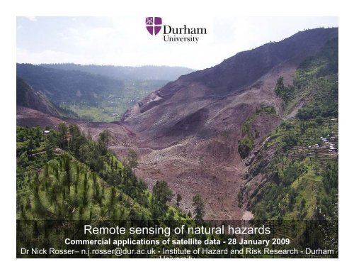
<strong>Remote</strong> <strong>sensing</strong> <strong>of</strong> <strong>natural</strong> <strong>hazards</strong><br />
Commercial applications <strong>of</strong> satellite data - 28 January 2009<br />
Dr Nick Rosser– n.j.rosser@dur.ac.uk - Institute <strong>of</strong> Hazard and Risk Research - Durham<br />
University
<strong>Remote</strong> Sensing & Natural Hazards<br />
Research<br />
• Introduction to IHRR<br />
– Combine social & physical approaches to<br />
understanding hazard & risk<br />
– ‘Global South’ focus<br />
– Applied & responsive research<br />
– Flooding, EQs & Landslides<br />
• IHRR application <strong>of</strong> RS to NH research<br />
• Process understanding &modelling<br />
• Linking process to earth observation<br />
• Prediction &upscaling<br />
– Coastal change<br />
– Post-earthquake sedimentation<br />
www.dur.ac.uk/ihrr<br />
• Future research directions &<br />
challenges<br />
Hazards research v <strong>hazards</strong> impact
Monitoring processes<br />
Rock cliff retreat – influence <strong>of</strong> precision<br />
• Challenges . . .<br />
– Input data for coastline retreat prediction<br />
– Poor quality monitoring data, looking in the<br />
wrong direction?<br />
– Resolution & sampling frequency<br />
• Integrating air-borne with terrestrial remote<br />
<strong>sensing</strong> data to better interpret remote<br />
<strong>sensing</strong> data<br />
• 3D laser scanning survey at 0.01 m<br />
resolution, over > 50,000 m 2 <strong>of</strong> cliff face<br />
• 3D modelling <strong>of</strong> scan data can detect 3D<br />
change to the cliff face < 0.0001 m 3
3D data processing &rockfall geometry extraction<br />
NJ Rosser, DN Petley, M. Lim, SA Dunning & RJ Allison 2005 Terrestrial laser scanning for monitoring the process <strong>of</strong><br />
hard rock coastal cliff erosion Quarterly Journal <strong>of</strong> Engineering Geology and Hydrogeology, 38, 363–375
Reassessing retreat<br />
654,373 rockfalls monitored over 5 years (mean = 0.001 m 3 , largest = 2,500 m 3 )<br />
Aggregate recession rate = 0.01 m/yr (published rate = 0.1 m/yr)<br />
Predicted 100 yr retreat = 3.6 m (published prediction 100 yr retreat – 90 m)
Sea-level control on cliff erosion rate?<br />
3D data processing &rockfall geometry extraction<br />
NJ Rosser, DN Petley, M. Lim, SA Dunning & RJ Allison 2005 Terrestrial laser scanning for monitoring the process <strong>of</strong><br />
hard rock coastal cliff erosion Quarterly Journal <strong>of</strong> Engineering Geology and Hydrogeology, 38, 363–375
Environmental control on rockfall occurrence?<br />
3D data processing &rockfall geometry extraction<br />
NJ Rosser, DN Petley, M. Lim, SA Dunning & RJ Allison 2005 Terrestrial laser scanning for monitoring the process <strong>of</strong><br />
hard rock coastal cliff erosion Quarterly Journal <strong>of</strong> Engineering Geology and Hydrogeology, 38, 363–375<br />
Squares represent 11 m x 11 m <strong>of</strong> cliff face, at monthly<br />
survey intervals
Precursors & failure prediction?<br />
•3D assessment identifies precursors<br />
•Potential to predict v forecast<br />
•Applied more widely to:<br />
•Embankments<br />
•Mine high-walls<br />
•Permanent monitoring<br />
3D data processing &rockfall geometry extraction<br />
Rosser, N.J., Lim, N, Petley, D.N., Dunning, S. & Allison, R.J. 2007 Patterns <strong>of</strong> precursory rockfall prior to slope failure.<br />
Journal <strong>of</strong> Geophysical Research.<br />
Squares represent 11 m x 11 m <strong>of</strong> cliff face, at monthly<br />
survey intervals
Post-earthquake<br />
landslides &<br />
sedimentation<br />
•EQ triggered landslide<br />
potentially hold great insight<br />
into earthquake dynamics &<br />
prediction<br />
•History <strong>of</strong> extreme postearthquake<br />
landscape change<br />
& sedimentation<br />
Sichuan<br />
2008<br />
(after, Bilham (2007))<br />
•What is the likely future nature<br />
<strong>of</strong> sediment dynamics in post-<br />
EQ Sichuan?<br />
Challenges:<br />
•Limited image availability<br />
•Topography<br />
•Monsoon<br />
•Politically sensitive<br />
(after, Keefer (1990))
Post 1999 Chi Chi, Taiwan river-bed<br />
aggradation<br />
1998<br />
2005<br />
2004
Post-earthquake<br />
sedimentation –<br />
Sichuan?<br />
17 June<br />
18 Nov<br />
Aggradation <strong>of</strong> >10 m in Beichuan in 5<br />
months, due to landslide remobilization
Steep topography - Poor lighting - Monsoon conditions - Data access<br />
http://www.eeri.org/site/images/lfe/china_20080512_zwang.ppt
http://www.eeri.org/site/images/lfe/china_20080512_zwang.ppt<br />
Continuing collapse – Monsoon driven failure<br />
http://www.eeri.org/site/images/lfe/china_20080512_zwang.ppt
Combined use <strong>of</strong> ALOS, EO1, QB, & SPOT imagery
Post-EQ<br />
sedimentation<br />
Automatic landslide mapping<br />
Combined multispectral analysis, using a<br />
range <strong>of</strong> available satellite imagery:<br />
•SPOT, IKONOS, LANDSAT, ALOS,<br />
EO1<br />
•Develop combine topographic / spectral<br />
model to classify landslides<br />
•Repeat over successive images<br />
Model <strong>of</strong> landslide distribution based<br />
upon:<br />
•Topographic amplification (DEM)<br />
•Slope / curvature<br />
•Ground cover (SPOT)<br />
Future EQ landslide prediction
30 % ground surface failed, > 100,000 landslides mapped, to date > 40,000<br />
reactivated
Post-EQ sedimentation<br />
Automatic landslide mapping<br />
•Modelled landslide<br />
distribution<br />
•Demonstrates limits<br />
to image resolution<br />
•Model transfer to<br />
other examples
Future research directions<br />
• Combining ground-based<br />
observations with wide-scale air<br />
&space-bourne monitoring<br />
• TLS, GB-InSAR<br />
• Potential for rapid assessment<br />
• Move towards predictive<br />
monitoring:<br />
• PSInSAR, TRMM, TLS<br />
• Temporal & spatial resolution<br />
• ? = ???????
www.dur.ac.uk/ihrr<br />
<strong>Remote</strong> <strong>sensing</strong> <strong>of</strong> <strong>natural</strong> <strong>hazards</strong><br />
Commercial applications <strong>of</strong> satellite data - 28 January 2009<br />
Dr Nick Rosser – n.j.rosser@dur.ac.uk - Institute <strong>of</strong> Hazard and Risk Research - Durham University
Flood modelling<br />
Why do we need satellite<br />
imagery for flood<br />
inundation modelling?<br />
1. Source <strong>of</strong> boundary<br />
condition data<br />
•Topography, especially<br />
given finer resolution models<br />
where topographic data<br />
handling is spatially explicit<br />
(e.g. 1.0 m resolution)<br />
•Friction, especially as it is<br />
controlled by land-use<br />
cover, although both<br />
theoretical arguments and<br />
sensitivity analysis points to<br />
inundation being less<br />
sensitive to floodplain<br />
friction but very sensitive to<br />
in-channel friction)<br />
York floods, 2000
2. In model parameterisation . . .<br />
• All flood inundation<br />
models are simplifications<br />
<strong>of</strong> the governing<br />
processes<br />
• Results in parameters<br />
with uncertain physical<br />
meaning (e.g. roughness)<br />
as they are effective<br />
• Need predictions that can<br />
be used to constrain<br />
those parameters<br />
• Inundation extent is really<br />
useful here<br />
York floods, 2000<br />
Yu, D. & Lane, S. 2005. Urban flood modelling using a 2-dimensional diffusionwave<br />
treatment. Hydrological Processes
3. For model validation<br />
100<br />
90<br />
Subject to data not being used in<br />
parameterisation, as a means <strong>of</strong><br />
assessing model performance<br />
Important when assessing<br />
different models<br />
Model performance<br />
80<br />
70<br />
60<br />
50<br />
40<br />
30<br />
Accuracy<br />
Conditional Kappa<br />
(for wet cells)<br />
4<br />
8<br />
16<br />
32<br />
32 m<br />
16 m<br />
8 m<br />
4 m