On the Fractional Order Control of Heat Systems
On the Fractional Order Control of Heat Systems
On the Fractional Order Control of Heat Systems

You also want an ePaper? Increase the reach of your titles
YUMPU automatically turns print PDFs into web optimized ePapers that Google loves.
<strong>On</strong> <strong>the</strong> <strong>Fractional</strong> <strong>Order</strong> <strong>Control</strong> <strong>of</strong> <strong>Heat</strong> <strong>Systems</strong><br />
Isabel S. Jesus, J. A. Tenreiro Machado, and Ramiro S. Barbosa<br />
Institute <strong>of</strong> Engineering <strong>of</strong> Porto, Department <strong>of</strong> Electrotechnical Engineering<br />
Rua Dr. António Bernardino de Almeida, n. 431, 4200-072 Porto, Portugal<br />
{isj, jtm, rsb}@isep.ipp.pt<br />
Summary. The differentiation <strong>of</strong> non-integer order has its origin in <strong>the</strong> seventeenth century,<br />
but only in <strong>the</strong> last two decades appeared <strong>the</strong> first applications in <strong>the</strong> area <strong>of</strong> control <strong>the</strong>ory.<br />
In this paper we consider <strong>the</strong> study <strong>of</strong> a heat diffusion system based on <strong>the</strong> application <strong>of</strong><br />
<strong>the</strong> fractional calculus concepts. In this perspective, several control methodologies are investigated<br />
namely <strong>the</strong> fractional PID and <strong>the</strong> Smith predictor. Extensive simulations are presented<br />
assessing <strong>the</strong> performance <strong>of</strong> <strong>the</strong> proposed fractional-order algorithms.<br />
1 Introduction<br />
<strong>Fractional</strong> calculus (FC) is a generalization <strong>of</strong> integration and differentiation to a complex order<br />
α, being <strong>the</strong> fundamental operator a D α t ,wherea and t are <strong>the</strong> limits <strong>of</strong> <strong>the</strong> operation [1,2].<br />
The FC concepts constitute a useful tool to describe several physical phenomena, such as heat,<br />
flow, electricity, magnetism, mechanics or fluid dynamics and presently it is applied in almost<br />
all areas <strong>of</strong> science and engineering.<br />
In <strong>the</strong> last years, FC has been used increasingly to model <strong>the</strong> constitutive behavior <strong>of</strong> materials<br />
and physical systems exhibiting hereditary and memory properties. This is <strong>the</strong> main<br />
advantage <strong>of</strong> fractional-order derivatives in comparison with classical integer-order models,<br />
where <strong>the</strong>se effects are neglected.<br />
It is well-known that <strong>the</strong> fractional-order operator s 0.5 appears in several types <strong>of</strong> problems<br />
[3]. The transmission lines, <strong>the</strong> heat flow or <strong>the</strong> diffusion <strong>of</strong> neutrons in a nuclear reactor<br />
are examples where <strong>the</strong> half-operator is <strong>the</strong> fundamental element. <strong>On</strong> <strong>the</strong> o<strong>the</strong>r hand, diffusion<br />
is one <strong>of</strong> <strong>the</strong> three fundamental partial differential equations <strong>of</strong> ma<strong>the</strong>matical physics [4].<br />
In this paper we investigate <strong>the</strong> heat diffusion system in <strong>the</strong> perspective <strong>of</strong> applying <strong>the</strong><br />
FC <strong>the</strong>ory. Several control strategies based on fractional-order algorithms are presented and<br />
compared with <strong>the</strong> classical schemes. The adoption <strong>of</strong> fractional-order controllers has been<br />
justified by its superior performance, particularly when used with fractional-order dynamical<br />
systems, such as <strong>the</strong> case <strong>of</strong> <strong>the</strong> heat system under study. The fractional-order PID (PI α D β<br />
controller) involves an integrator <strong>of</strong> order α ∈ R+ and a differentiator <strong>of</strong> order β ∈ R+. It<br />
J.A.T. Machado et al. (eds.), Intelligent Engineering <strong>Systems</strong> and Computational Cybernetics,<br />
c○ Springer Science+Business Media LLC 2008
376 Isabel S. Jesus, J. A. Tenreiro Machado, and Ramiro S. Barbosa<br />
was demonstrated <strong>the</strong> good performance <strong>of</strong> this type <strong>of</strong> controller, in comparison with <strong>the</strong><br />
conventional PID algorithms.<br />
Bearing <strong>the</strong>se ideas in mind, <strong>the</strong> paper is organized as follows. Section 2 gives <strong>the</strong> fundamentals<br />
<strong>of</strong> fractional-order control systems. Section 3 introduces <strong>the</strong> heat diffusion system.<br />
Section 4 points out several control strategies for <strong>the</strong> heat system and discusses <strong>the</strong>ir<br />
results. Finally, Section 5 draws <strong>the</strong> main conclusions and addresses perspectives towards future<br />
developments.<br />
2 <strong>Fractional</strong>-<strong>Order</strong> <strong>Control</strong> <strong>Systems</strong><br />
<strong>Fractional</strong>-order control systems are characterized by differential equations that have, in <strong>the</strong><br />
dynamical system and/or in <strong>the</strong> control algorithm, an integral and/or a derivative <strong>of</strong> fractionalorder.<br />
Due to <strong>the</strong> fact that <strong>the</strong>se operators are defined by irrational continuous transfer functions,<br />
in <strong>the</strong> Laplace domain, or infinite dimensional discrete transfer functions, in <strong>the</strong> Z<br />
domain, we <strong>of</strong>ten encounter evaluation problems in <strong>the</strong> simulations. Therefore, when analyzing<br />
fractional-order systems, we usually adopt continuous or discrete integer-order approximations<br />
<strong>of</strong> fractional-order operators [5–7].<br />
The ma<strong>the</strong>matical definition <strong>of</strong> a fractional-order derivative and integral has been <strong>the</strong> subject<br />
<strong>of</strong> several different approaches [1, 2]. <strong>On</strong>e commonly used definition for <strong>the</strong> fractionalorder<br />
derivative is given by <strong>the</strong> Riemann–Liouville definition (α > 0):<br />
aDt α 1 d n ∫ t f (τ)<br />
f (t)=<br />
Γ (n − α) dt n dτ, n − 1 < α < n, (1)<br />
a<br />
α−n+1<br />
(t − τ)<br />
where f (t) is <strong>the</strong> applied function and Γ (x) is <strong>the</strong> Gamma function <strong>of</strong> x. Ano<strong>the</strong>r widely used<br />
definition is given by <strong>the</strong> Grünwald–Letnikov approach (α ∈ R):<br />
h ]<br />
[<br />
aDt α 1<br />
t−a (<br />
f (t)=lim h→0 h<br />
∑ α (−1) k α<br />
k<br />
k=0<br />
( ) α<br />
=<br />
k<br />
Γ (α + 1)<br />
Γ (k + 1)Γ (α − k + 1)<br />
)<br />
f (t − kh)<br />
where h is <strong>the</strong> time increment and [x] means <strong>the</strong> integer part <strong>of</strong> x.<br />
The “memory” effect <strong>of</strong> <strong>the</strong>se operators is demonstrated by (1) and (2), where <strong>the</strong> convolution<br />
integral in (1) and <strong>the</strong> infinite series in (2), reveal <strong>the</strong> unlimited memory <strong>of</strong> <strong>the</strong>se operators,<br />
ideal for modeling hereditary and memory properties in physical systems and materials.<br />
An alternative definition to (1) and (2), which reveals useful for <strong>the</strong> analysis <strong>of</strong> fractionalorder<br />
control systems, is given by <strong>the</strong> Laplace transform method. Considering vanishing<br />
initial conditions, <strong>the</strong> fractional differintegration is defined in <strong>the</strong> Laplace domain, F(s) =<br />
L{ f (t)},as:<br />
L{ a Dt α f (t)} = s α F (s), α ∈ R (3)<br />
An important aspect <strong>of</strong> fractional-order algorithms can be illustrated through <strong>the</strong> elemental<br />
control system with open-loop transfer function G(s)=Ks −α (1 < α < 2) in <strong>the</strong> forward<br />
path and unit feedback. The open-loop Bode diagrams <strong>of</strong> amplitude and phase have a slope <strong>of</strong><br />
−20α dB/dec and a constant phase <strong>of</strong> −απ/2 rad over <strong>the</strong> entire frequency domain. Therefore,<br />
<strong>the</strong> closed-loop system has a constant phase margin <strong>of</strong> PM = π (1 − α/2) rad that is<br />
independent <strong>of</strong> <strong>the</strong> system gain K. Therefore, <strong>the</strong> closed-loop system will be robust against<br />
gain variations exhibiting step responses with an iso-damping property [8].<br />
(2a)<br />
(2b)
<strong>On</strong> <strong>the</strong> <strong>Fractional</strong> <strong>Order</strong> <strong>Control</strong> <strong>of</strong> <strong>Heat</strong> <strong>Systems</strong> 377<br />
In this paper we adopt discrete integer-order approximations to <strong>the</strong> fundamental element<br />
s α (α ∈ R) <strong>of</strong> a fractional-order control (FOC) strategy. The usual approach for obtaining<br />
discrete equivalents <strong>of</strong> continuous operators <strong>of</strong> type s α adopts <strong>the</strong> Euler, Tustin and Al-Alaoui<br />
generating functions [5].<br />
It is well known that rational-type approximations frequently converge faster than polynomial-type<br />
approximations and have a wider domain <strong>of</strong> convergence in <strong>the</strong> complex domain.<br />
Thus, by using <strong>the</strong> Euler operator w(z −1 )=(1 − z −1 )/T , and performing a power series expansion<br />
<strong>of</strong> [ w(z −1 ) ] α [<br />
= (1−z −1 )/T ] α gives <strong>the</strong> discretization formula corresponding to <strong>the</strong><br />
Grünwald–Letnikov definition (2):<br />
(<br />
D α z −1) ( 1 − z −1 ) α ∞<br />
=<br />
= h α (k)z −k<br />
(4a)<br />
(<br />
h α 1<br />
(k)=<br />
T<br />
T<br />
∑<br />
k=0<br />
) α ( ) k − α − 1<br />
k<br />
where <strong>the</strong> impulse response sequence h α (k) is given by <strong>the</strong> expression (4b) (k ≥ 0).<br />
A rational-type approximation can be obtained by applying <strong>the</strong> Padé approximation<br />
method to <strong>the</strong> impulse response sequence (4b) h α (k), yielding <strong>the</strong> discrete transfer function:<br />
H<br />
(z −1) = b 0 + b 1 z −1 + ...+ b m z −m ∞<br />
1 + a 1 z −1 + ...+ a n z −n = ∑ h(k)z −k , (5)<br />
k=0<br />
where m ≤ n and <strong>the</strong> coefficients a k and b k are determined by fitting <strong>the</strong> first m + n + 1values<br />
<strong>of</strong> h α (k) into <strong>the</strong> impulse response h(k) <strong>of</strong> <strong>the</strong> desired approximation H(z −1 ). Thus, we obtain<br />
an approximation that has a perfect match to <strong>the</strong> desired impulse response h α (k) for <strong>the</strong> first<br />
m + n + 1values<strong>of</strong>k [8]. Note that <strong>the</strong> above Padé approximation is obtained by considering<br />
<strong>the</strong> Euler operator but <strong>the</strong> determination process will be exactly <strong>the</strong> same for o<strong>the</strong>r types <strong>of</strong><br />
discretization schemes.<br />
(4b)<br />
3 <strong>Heat</strong> Diffusion<br />
The heat diffusion is governed by a linear partial differential equation (PDE) <strong>of</strong> <strong>the</strong> form:<br />
(<br />
∂u ∂ 2<br />
∂t = k u<br />
∂x 2 + ∂ 2 u<br />
∂y 2 + ∂ 2 )<br />
u<br />
∂z 2 , (6)<br />
where k is <strong>the</strong> diffusivity, t is <strong>the</strong> time, u is <strong>the</strong> temperature and (x,y,z) are <strong>the</strong> space cartesian<br />
coordinates. The system (6) involves <strong>the</strong> solution <strong>of</strong> a PDE <strong>of</strong> parabolic type for which <strong>the</strong><br />
standard <strong>the</strong>ory guarantees <strong>the</strong> existence <strong>of</strong> a unique solution [9].<br />
For <strong>the</strong> case <strong>of</strong> a planar perfectly isolated surface we usually apply a constant temperature<br />
U 0 at x = 0 and we analyze <strong>the</strong> heat diffusion along <strong>the</strong> horizontal coordinate x. Under <strong>the</strong>se<br />
conditions, <strong>the</strong> heat diffusion phenomenon is described by a non-integer order model, yielding:<br />
U (x,s)= U 0<br />
s G(s), G(s)=e−x√ s<br />
k , (7)<br />
where x is <strong>the</strong> space coordinate, U 0 is <strong>the</strong> boundary condition and G(s) is <strong>the</strong> system transfer<br />
function.<br />
In our study, <strong>the</strong> simulation <strong>of</strong> <strong>the</strong> heat diffusion is performed by adopting <strong>the</strong> Crank–<br />
Nicholson implicit numerical integration based on <strong>the</strong> discrete approximation to differentiation<br />
[10–13].
378 Isabel S. Jesus, J. A. Tenreiro Machado, and Ramiro S. Barbosa<br />
4 <strong>Control</strong> Strategies for <strong>Heat</strong> Diffusion <strong>Systems</strong><br />
In this section we consider three strategies for <strong>the</strong> control <strong>of</strong> <strong>the</strong> heat diffusion system. In <strong>the</strong><br />
first two subsections, we analyze <strong>the</strong> system <strong>of</strong> Fig. 1 by adopting classical PID and fractional<br />
PID β controllers, respectively. In <strong>the</strong> third subsection we use a Smith predictor (SP) structure<br />
with a fractional PID β controller (Fig. 5).<br />
Fig. 1: Closed-loop system with PID or PID β controller G c (s)<br />
The generalized PID controller G c (s) has a transfer function <strong>of</strong> <strong>the</strong> form:<br />
[<br />
G c (s)=K 1 + 1 ]<br />
T i s α + T ds β , (8)<br />
where α and β are <strong>the</strong> orders <strong>of</strong> <strong>the</strong> fractional integrator and differentiator, respectively. The<br />
constants K, T i and T d are correspondingly <strong>the</strong> proportional gain, <strong>the</strong> integral time constant<br />
and <strong>the</strong> derivative time constant.<br />
Clearly, taking (α, β) = {(1, 1), (1, 0), (0, 1), (0, 0)} we get <strong>the</strong> classical {PID, PI, PD, P}<br />
controllers, respectively. O<strong>the</strong>r PID controllers are possible, namely: PD β controller, PI α controller,<br />
PID β controller, and so on. The PI α D β controller is more flexible and gives <strong>the</strong> possibility<br />
<strong>of</strong> adjusting more carefully <strong>the</strong> closed-loop system characteristics.<br />
4.1 The PID <strong>Control</strong>ler<br />
In this subsection we analyze <strong>the</strong> closed-loop system with a conventional PID controller given<br />
by <strong>the</strong> transfer function (8) with α = β = 1. Often, <strong>the</strong> PID parameters (K, T i , T d ) are tuned<br />
by using <strong>the</strong> so-called Ziegler–Nichols open loop (ZNOL) method. The ZNOL heuristics are<br />
based on <strong>the</strong> approximate first-order plus dead-time model:<br />
Ĝ(s)=<br />
K p<br />
τs + 1 e−sT (9)<br />
A step input is applied at x = 0.0 m and <strong>the</strong> output c(t) analyzed for x = 3.0 m, without <strong>the</strong><br />
saturation. The resulting parameters are {K p ,τ,T} = {0.52, 162,28} leading to <strong>the</strong> PID constants<br />
{K, T i , T d } = {18.07, 34.0, 8.5}. We verify that <strong>the</strong> system with a PID controller, tuned<br />
according with <strong>the</strong> ZNOL heuristics, does not produce satisfactory results giving a significant<br />
overshoot, and a large settling time. Moreover, <strong>the</strong> step response reveals a considerable time<br />
delay. The poor results obtained indicate that <strong>the</strong> method <strong>of</strong> tuning as well <strong>the</strong> structure <strong>of</strong> <strong>the</strong><br />
system may not be <strong>the</strong> most adequate for <strong>the</strong> control <strong>of</strong> <strong>the</strong> heat system under consideration.<br />
In fact, <strong>the</strong> inherent fractional-order dynamics <strong>of</strong> <strong>the</strong> system lead us to consider o<strong>the</strong>r configurations.<br />
In this perspective, we propose <strong>the</strong> use <strong>of</strong> fractional-order controllers and <strong>the</strong> SP to<br />
achieve a superior control performance.
<strong>On</strong> <strong>the</strong> <strong>Fractional</strong> <strong>Order</strong> <strong>Control</strong> <strong>of</strong> <strong>Heat</strong> <strong>Systems</strong> 379<br />
4.2 The PID β <strong>Control</strong>ler<br />
In this subsection we analyze <strong>the</strong> closed-loop system with a PID β controller given by <strong>the</strong><br />
transfer function (8) with α = 1. The fractional-order derivative term T d s β in (8) is implemented<br />
by using a fourth-order Padé discrete rational transfer function <strong>of</strong> type (5). It is used a<br />
sampling period <strong>of</strong> T = 0.1s.<br />
The PID β controller is tuned by minimization <strong>of</strong> an integral performance index. For that,<br />
we adopt <strong>the</strong> integral square error (ISE) and <strong>the</strong> integral time square error (ITSE) criteria<br />
defined as:<br />
∫ ∞<br />
ISE = [r (t) − c(t)] 2 dt (10)<br />
0<br />
∫ ∞<br />
ITSE = t [r (t) − c(t)] 2 dt (11)<br />
0<br />
10 2<br />
K<br />
T i<br />
K - ISE<br />
K - ITSE<br />
10 0<br />
0 0.1 0.2 0.3 0.4 0.5 0.6 0.7 0.8 0.9 1<br />
10 1 β<br />
T i<br />
- ISE<br />
T i - ITSE<br />
10 1<br />
0 0.1 0.2 0.3 0.4 0.5 0.6 0.7 0.8 0.9 1<br />
β<br />
(a)<br />
(b)<br />
10 2 0 0.1 0.2 0.3 0.4 0.5 0.6 0.7 0.8 0.9 1<br />
10 1<br />
T d<br />
10 0<br />
10 −1<br />
β<br />
T d<br />
- ISE<br />
T d<br />
- ITSE<br />
(c)<br />
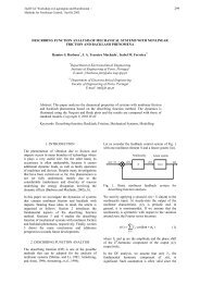
Fig. 2: The PID β parameters (K, T i, T d ) versus β for <strong>the</strong> ISE and <strong>the</strong> ITSE criteria
380 Isabel S. Jesus, J. A. Tenreiro Machado, and Ramiro S. Barbosa<br />
We can use o<strong>the</strong>r integral performance criteria such as <strong>the</strong> integral absolute error (IAE)<br />
or <strong>the</strong> integral time absolute error (ITAE) but <strong>the</strong> ISE and <strong>the</strong> ITSE criteria have produced <strong>the</strong><br />
best results. Fur<strong>the</strong>rmore, <strong>the</strong> ITSE criterion enable us to study <strong>the</strong> influence <strong>of</strong> time in <strong>the</strong><br />
error generated by <strong>the</strong> system.<br />
A step reference input R(s) =1/s is applied at x = 0.0 m and <strong>the</strong> output c(t) is analyzed for<br />
x = 3.0 m, without considering saturation. The heat system is simulated for 3,000 s. Figure 2<br />
illustrates <strong>the</strong> variation <strong>of</strong> <strong>the</strong> fractional PID parameters (K, T i , T d ) as function <strong>of</strong> <strong>the</strong> order’s<br />
derivative β, tuned according with <strong>the</strong> ISE and <strong>the</strong> ITSE criteria.<br />
The curves reveal that for β < 0.4, <strong>the</strong> parameters (K, T i , T d ) are slightly different, for<br />
<strong>the</strong> two ISE and ITSE criteria, but for β ≥ 0.4 <strong>the</strong>y almost lead to similar values. This fact<br />
indicates a large influence <strong>of</strong> a weak order derivative on system’s dynamics.<br />
To fur<strong>the</strong>r illustrate <strong>the</strong> performance <strong>of</strong> <strong>the</strong> fractional-order controllers a saturation nonlinearity<br />
is included in <strong>the</strong> closed-loop system <strong>of</strong> Fig. 1 and inserted in series with <strong>the</strong> output<br />
<strong>of</strong> <strong>the</strong> PID controller G c (s). The saturation element is defined as:<br />
⎧<br />
⎨ +δ, m > δ<br />
n(m)= m, |m| ≤ δ<br />
⎩<br />
−δ, m < −δ<br />
The controller performance is evaluated for δ = {20,...,100,∞}, where <strong>the</strong> last case corresponds<br />
to a system without saturation. We use <strong>the</strong> same fractional-PID parameters obtained<br />
without considering <strong>the</strong> saturation nonlinearity.<br />
10 6<br />
β = 1<br />
β = 0.875<br />
β = 1<br />
β = 0.85<br />
Energy {m(t)}<br />
10 5<br />
δ =∞<br />
δ = 20<br />
Energy {m(t)}<br />
10 5<br />
δ = ∞<br />
10 6 ITSE {c(t )}<br />
δ = 20<br />
10 4 16 17 18 19 20 21 22 23 24 25 26<br />
10 4 150 200 250 300 350 400 450<br />
β = 0<br />
β = 0<br />
ISE {c(t)}<br />
(a)<br />
(b)<br />
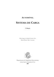
Fig. 3: Energy E m versus <strong>the</strong> ISE and <strong>the</strong> ITSE for δ = {20,...,100,∞},0≤ β ≤ 1<br />
The energy E m at <strong>the</strong> output m(t) <strong>of</strong> <strong>the</strong> fractional PID controller is also analyzed through<br />
<strong>the</strong> expression:<br />
∫ T s<br />
E m = m 2 (t)dt, (12)<br />
0<br />
where T s is <strong>the</strong> time corresponding to <strong>the</strong> 5% settling time criterion <strong>of</strong> <strong>the</strong> system output c(t).
<strong>On</strong> <strong>the</strong> <strong>Fractional</strong> <strong>Order</strong> <strong>Control</strong> <strong>of</strong> <strong>Heat</strong> <strong>Systems</strong> 381<br />
1.2<br />
1<br />
δ = 20<br />
1.2<br />
1<br />
δ = ∞<br />
0.8<br />
0.8<br />
c(t)<br />
0.6<br />
c(t)<br />
0.6<br />
0.4<br />
0.4<br />
0.2<br />
ISE - β = 0.875<br />
ITSE - β = 0.85<br />
0<br />
0 100 200 300 400 500<br />
time [s]<br />
0.2<br />
ISE - β = 0.875<br />
ITSE - β = 0.85<br />
0<br />
0 50 100 150 200 250 300 350 400 450 500<br />
time [s]<br />
(a)<br />
(b)<br />
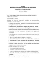
Fig. 4: Step responses <strong>of</strong> <strong>the</strong> closed-loop system for <strong>the</strong> ISE and <strong>the</strong> ITSE indices, with a PID β<br />
controller, for δ = {20,∞} and x = 3.0m<br />
<strong>Control</strong>ler<br />
R(s) + E 1 + E 2 M (s)<br />
G c (s)<br />
− −<br />
Saturation<br />
δ<br />
1 N(s)<br />
δ<br />
<strong>Heat</strong> System<br />
G (s)<br />
C (s)<br />
^<br />
G (s)<br />
B m<br />
e -Ts<br />
−<br />
+<br />
Model<br />
Delay<br />
E m<br />
Fig. 5: Closed-loop system with a Smith predictor and a PID β controller G c (s)<br />
Figure 3 depicts <strong>the</strong> energy E m as function <strong>of</strong> <strong>the</strong> ISE and <strong>the</strong> ITSE indices for 0 ≤ β ≤ 1.<br />
As can be seen, <strong>the</strong> energy changes smoothly for different values <strong>of</strong> δ when considering a<br />
given order β. However, fixing <strong>the</strong> value δ, we verify that <strong>the</strong> energy increases significantly<br />
with β.<br />
<strong>On</strong> <strong>the</strong> o<strong>the</strong>r hand, we observe that <strong>the</strong> ISE decreases with δ for β ≤ 0.875, while for<br />
β > 0.875 <strong>the</strong> ISE increases very quickly. The same conclusions can be outlined relatively to<br />
<strong>the</strong> ITSE criterion. The results confirm <strong>the</strong> good performance <strong>of</strong> <strong>the</strong> system for low values <strong>of</strong><br />
<strong>the</strong> fractional-order derivative term.<br />
When comparing <strong>the</strong> two indices, we also note that <strong>the</strong> value <strong>of</strong> <strong>the</strong> ITSE is generally<br />
larger than <strong>the</strong> corresponding for <strong>the</strong> ISE case. This occurs because <strong>of</strong> <strong>the</strong> large simulation<br />
time needed to stabilize <strong>the</strong> system, which is T s ∼ 700 s.<br />
Figure 4 shows <strong>the</strong> step responses <strong>of</strong> <strong>the</strong> closed-loop system for <strong>the</strong> PID β tuned in <strong>the</strong><br />
perspective <strong>of</strong> ISE and ITSE.<br />
The controller parameters {K, T i , T d , β} correspond to <strong>the</strong> minimization <strong>of</strong> those indices<br />
leading to <strong>the</strong> values ISE: {K,T i ,T d ,β}≡{3,23,90.6,0.875} and ITSE: {K,T i ,T d ,β}≡<br />
{1.8,17.6,103.6,0.85}.<br />
The step responses reveal a large diminishing <strong>of</strong> <strong>the</strong> overshoot and <strong>the</strong> rise time when<br />
compared with <strong>the</strong> integer PID, showing a good transient response and a zero steady-state<br />
error. As should be expected, <strong>the</strong> PID β leads to better results than <strong>the</strong> PID controller tuned
382 Isabel S. Jesus, J. A. Tenreiro Machado, and Ramiro S. Barbosa<br />
10 2<br />
10 2 (a)<br />
10 1 β<br />
K<br />
T i<br />
K - ISE<br />
K - ITSE<br />
10 1<br />
0 0.1 0.2 0.3 0.4 0.5 0.6 0.7 0.8 0.9 1<br />
β<br />
T i - ISE<br />
T i<br />
- ITSE<br />
10 0<br />
0 0.1 0.2 0.3 0.4 0.5 0.6 0.7 0.8 0.9 1<br />
(b)<br />
T d<br />
10 −1<br />
10 1<br />
10 0<br />
T d - ISE<br />
T d - ITSE<br />
10 −2<br />
0 0.1 0.2 0.3 0.4 0.5 0.6 0.7 0.8 0.9 1<br />
β<br />
(c)<br />
Fig. 6: The PID β parameters (K, T i , T d ) versus β for <strong>the</strong> ISE and <strong>the</strong> ITSE criteria<br />
through <strong>the</strong> ZNOL method. These results demonstrate <strong>the</strong> effectiveness <strong>of</strong> <strong>the</strong> fractional-order<br />
algorithms when used for <strong>the</strong> control <strong>of</strong> fractional-order systems.<br />
4.3 The Smith Predictor with a PID β <strong>Control</strong>ler<br />
In this subsection we adopt a fractional PID β controller inserted in a SP structure, as represented<br />
in Fig. 5. This algorithm, developed by O. J. M. Smith in 1957, is a dead-time compensation<br />
technique, very effective in improving <strong>the</strong> control <strong>of</strong> processes having time delays<br />
[14, 15].<br />
The transfer function Ĝ(s), inserted in <strong>the</strong> second branch <strong>of</strong> <strong>the</strong> SP, is described by <strong>the</strong><br />
following first-order plus dead-time model:<br />
Ĝ(s)= 0.52<br />
162s + 1 e−28s (13)
<strong>On</strong> <strong>the</strong> <strong>Fractional</strong> <strong>Order</strong> <strong>Control</strong> <strong>of</strong> <strong>Heat</strong> <strong>Systems</strong> 383<br />
where <strong>the</strong> parameters (K p ,τ,T) =(0.52, 162, 28) were estimated by a least-squares fit<br />
between <strong>the</strong> frequency responses <strong>of</strong> <strong>the</strong> numerical model <strong>of</strong> <strong>the</strong> heat system and <strong>the</strong> SP<br />
model Ĝ(s).<br />
The PID β controller is tuned by applying <strong>the</strong> ISE and <strong>the</strong> ITSE integral performance criteria,<br />
as described in <strong>the</strong> previous subsection.<br />
10 4.3 ISE {c(t)}<br />
10 5 ITSE {c(t )}<br />
β = 0.8<br />
β = 0.8<br />
β = 1<br />
Energy {m(t)}<br />
10 4.2<br />
10 4.1<br />
δ = ∞<br />
δ = 20<br />
β = 1<br />
β = 0<br />
β = 1<br />
β = 0<br />
10 4<br />
17.5 18 18.5 19 19.5 20<br />
Energy {m(t)}<br />
δ = ∞<br />
δ = 20<br />
β = 0.7<br />
10 4 β = 0.5<br />
β = 0<br />
190 200 210 220 230<br />
(a)<br />
(b)<br />
Fig. 7: Energy E m versus <strong>the</strong> ISE and <strong>the</strong> ITSE indices for δ = {20,...,100,∞},0≤ β ≤ 1<br />
Figure 6 illustrates <strong>the</strong> variation <strong>of</strong> <strong>the</strong> PID β parameters (K, T i , T d ) as function <strong>of</strong> <strong>the</strong><br />
order’s derivative β, for <strong>the</strong> ISE and <strong>the</strong> ITSE indices, without <strong>the</strong> occurrence <strong>of</strong> saturation.<br />
1.2<br />
δ = 20<br />
1.2<br />
δ = ∞<br />
1<br />
1<br />
0.8<br />
0.8<br />
c (t)<br />
0.6<br />
c ( t)<br />
0.6<br />
0.4<br />
0.4<br />
0.2<br />
ISE Smith - β = 0.7<br />
ITSE Smith - β = 0.7<br />
0<br />
0 100 200 300 400 500<br />
time [s]<br />
0.2<br />
ISE Smith<br />
- β = 0.7<br />
ITSE Smith<br />
- β = 0.7<br />
0<br />
0 100 200 300 400 500<br />
time [s]<br />
(a)<br />
Fig. 8: Step responses <strong>of</strong> <strong>the</strong> closed-loop system for <strong>the</strong> PID β and <strong>the</strong> Smith predictor with<br />
PID β , for <strong>the</strong> ISE and <strong>the</strong> ITSE indices, δ = {20,∞}, x = 3.0m<br />
(b)
384 Isabel S. Jesus, J. A. Tenreiro Machado, and Ramiro S. Barbosa<br />
Figure 7 shows <strong>the</strong> relation between <strong>the</strong> energy E m and <strong>the</strong> values <strong>of</strong> <strong>the</strong> ISE and ITSE<br />
indices. We verify that <strong>the</strong> best case is achieved when β = 0.7, revealing that, with a SP structure,<br />
<strong>the</strong> effectiveness <strong>of</strong> <strong>the</strong> fractional-order controller is more evident.<br />
Since <strong>the</strong> effect <strong>of</strong> <strong>the</strong> system time delay is diminished by <strong>the</strong> use <strong>of</strong> <strong>the</strong> SP, <strong>the</strong> PID β controller<br />
and, more specifically, <strong>the</strong> fractional-order derivative D β will be more effective and,<br />
consequently, produce better results.<br />
Figure 8 illustrates <strong>the</strong> step responses for x = 3.0 m when applying a step input R(s)=1/s<br />
at x = 0.0 m, for <strong>the</strong> SP and <strong>the</strong> PID β controller with β = 0.7, both for <strong>the</strong> ISE and <strong>the</strong> ITSE<br />
indices. The graphs show a better transient response for <strong>the</strong> SP with a PID β , namely smaller<br />
values <strong>of</strong> <strong>the</strong> overshot, rise time and time delay. The settling time is approximately <strong>the</strong> same<br />
for both configurations.<br />
However, for small values <strong>of</strong> β, <strong>the</strong> step response <strong>of</strong> <strong>the</strong> SP is significantly better than <strong>the</strong><br />
corresponding one for <strong>the</strong> PID β controller. In <strong>the</strong> SP step response we still observe a time delay<br />
due to an insufficient match between <strong>the</strong> system model G(s) and <strong>the</strong> first-order approximation<br />
Ĝ(s). Therefore, for a superior use <strong>of</strong> this method a better approximation <strong>of</strong> <strong>the</strong> heat system<br />
should be envisaged. This subject, namely a fractional order SP model will be addressed in<br />
future research.<br />
5 Conclusions<br />
This paper presented <strong>the</strong> fundamental aspects <strong>of</strong> <strong>the</strong> FC <strong>the</strong>ory. We demonstrated that FC is a<br />
tool for modelling physical phenomena having superior capabilities than those <strong>of</strong> traditional<br />
methodologies. In this perspective, we studied a heat diffusion system, which is described<br />
through <strong>the</strong> fractional-order operator s 0.5 . The dynamics <strong>of</strong> <strong>the</strong> system was analyzed in <strong>the</strong><br />
perspective <strong>of</strong> FC, and some <strong>of</strong> its implications upon control algorithms and systems with<br />
time delay were also investigated.<br />
Acknowledgments<br />
The authors thank GECAD – Grupo de Investigação em Engenharia do Conhecimento e Apoio<br />
àDecisão, for <strong>the</strong> financial support to this work.<br />
References<br />
1. Oldham KB, Spanier J (1974) The <strong>Fractional</strong> Calculus. Academic, London<br />
2. Podlubny I (1999) <strong>Fractional</strong> Differential Equations. Academic, San Diego, CA<br />
3. Battaglia JL, Cois O, Puigsegur L, Oustaloup A (2001) Solving an inverse heat conduction<br />
problem using a non-integer identified model. International Journal <strong>of</strong> <strong>Heat</strong> and<br />
Mass Transfer 44:2671–2680<br />
4. Courant R, Hilbert D (1962) Methods <strong>of</strong> Ma<strong>the</strong>matical Physics, Partial Differential<br />
Equations. Wiley Interscience II, New York<br />
5. Barbosa RS, Machado JAT, Silva MF (2006) Time domain design <strong>of</strong> fractional differintegrators<br />
using least-squares. Signal Processing, EURASIP/Elsevier, 86(10):2567–2581<br />
6. Petras I, Vinagre BM (2002) Practical application <strong>of</strong> digital fractional order controller to<br />
temperature control. Acta Montanistica Slovaca 7(2):131–137
<strong>On</strong> <strong>the</strong> <strong>Fractional</strong> <strong>Order</strong> <strong>Control</strong> <strong>of</strong> <strong>Heat</strong> <strong>Systems</strong> 385<br />
7. Podlubny I, Petras I, Vinagre BM, Chen Y-Q, O’Leary P, Dorcak L (2003) Realization<br />
<strong>of</strong> fractional order controllers. Acta Montanistica Slovaca 8(3):233–235<br />
8. Barbosa RS, Machado JAT, Ferreira IM (2004) Tuning <strong>of</strong> PID controllers based on<br />
Bode’s ideal transfer function. Nonlinear Dynamics 38(1/4):305–321<br />
9. Machado JT, Jesus I, Boaventura Cunha J, Tar JK (2006) <strong>Fractional</strong> Dynamics and<br />
<strong>Control</strong> <strong>of</strong> Distributed Parameter <strong>Systems</strong>. In: Intelligent <strong>Systems</strong> at <strong>the</strong> Service <strong>of</strong><br />
Mankind. Vol 2, 295–305<br />
10. Crank J (1956) The Ma<strong>the</strong>matics <strong>of</strong> Diffusion. Oxford University Press, London<br />
11. Gerald CF, Wheatley PO (1999) Applied Numerical Analysis. Addison-Wesley, Reading,<br />
MA<br />
12. Jesus IS, Barbosa RS, Machado JAT, Cunha JB (2006) Strategies for <strong>the</strong> <strong>Control</strong> <strong>of</strong> <strong>Heat</strong><br />
Diffusion <strong>Systems</strong> Based on <strong>Fractional</strong> Calculus. In: IEEE International Conference on<br />
Computational Cybernetics. Estonia<br />
13. Jesus IS, Machado JAT, Cunha JB (2007) <strong>Fractional</strong> Dynamics and <strong>Control</strong> <strong>of</strong> <strong>Heat</strong><br />
Diffusion <strong>Systems</strong>. In: MIC 2007 – The 26th IASTED International Conference on<br />
Modelling, Identification and <strong>Control</strong>. Innsbruck, Austria<br />
14. Smith OJM (1957) Closed control <strong>of</strong> loops with dead time. Chemical Engineering<br />
Process 53:217–219<br />
15. Majhi S, A<strong>the</strong>rton DP (1999) Modified Smith predictor and controller for processes with<br />
time delay. IEE Proceedings or <strong>Control</strong> Theory and Applications 146(5):359–366