Modeling and Simulation of the LAUV Autonomous Underwater ...
Modeling and Simulation of the LAUV Autonomous Underwater ...
Modeling and Simulation of the LAUV Autonomous Underwater ...

Create successful ePaper yourself
Turn your PDF publications into a flip-book with our unique Google optimized e-Paper software.
<strong>Modeling</strong> <strong>and</strong> <strong>Simulation</strong> <strong>of</strong> <strong>the</strong> <strong>LAUV</strong> <strong>Autonomous</strong> <strong>Underwater</strong> Vehicle<br />
Jorge Estrela da Silva, Bruno Terra, Ricardo Martins <strong>and</strong> João Borges de Sousa<br />
Abstract— We derive <strong>the</strong> numerical coefficients for <strong>the</strong> nonlinear<br />
ma<strong>the</strong>matical model <strong>of</strong> a new AUV designed at Oporto<br />
University. This is made using <strong>the</strong>oretical <strong>and</strong> empirical methods<br />
as also by adapting <strong>the</strong> known results from similar AUVs.<br />
We use <strong>the</strong> derived model on MVS, a simulator which can be<br />
embedded in <strong>the</strong> loop <strong>of</strong> <strong>the</strong> control s<strong>of</strong>tware, by replacing <strong>the</strong><br />
interface with <strong>the</strong> sensors <strong>and</strong> actuators.<br />
Index Terms— <strong>Underwater</strong> Vehicles, <strong>Modeling</strong>, <strong>Simulation</strong><br />
I. INTRODUCTION<br />
On most methodologies, <strong>the</strong> design <strong>and</strong> tuning <strong>of</strong> controllers<br />
requires a ma<strong>the</strong>matical model <strong>of</strong> <strong>the</strong> system. We<br />
present a ma<strong>the</strong>matical model for <strong>the</strong> new generation <strong>of</strong><br />
autonomous underwater vehicles (AUV) designed <strong>and</strong> built at<br />
<strong>the</strong> <strong>Underwater</strong> Systems <strong>and</strong> Technology Laboratory (USTL)<br />
from Oporto University. These AUVs have a torpedo shape<br />
<strong>and</strong> <strong>the</strong>y are optimized for small size <strong>and</strong> low cost mechanical<br />
structure. The first vehicle <strong>of</strong> this generation is called<br />
<strong>LAUV</strong>. The ma<strong>the</strong>matical model will be employed on early<br />
testing <strong>of</strong> vehicle control s<strong>of</strong>tware.<br />
The computation <strong>of</strong> <strong>the</strong> coefficients <strong>of</strong> <strong>the</strong> nonlinear model<br />
is done by resorting to <strong>the</strong>oretical <strong>and</strong> empirical formulas<br />
<strong>and</strong> also by establishing analogies with known models from<br />
similar vehicles, namely <strong>the</strong> Isurus AUV, a REMUS class<br />
vehicle created at <strong>the</strong> Woods Hole Oceanographic Institution<br />
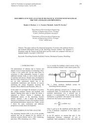
<strong>and</strong> customized at <strong>the</strong> USTL. Figure I shows both Isurus <strong>and</strong><br />
<strong>LAUV</strong>. The derived model will allow <strong>the</strong> tuning <strong>of</strong> controllers<br />
which, on <strong>the</strong>ir turn, will enable <strong>the</strong> execution <strong>of</strong> some inwater<br />
tests – such as operation at constant depth, far from<br />
<strong>the</strong> influence <strong>of</strong> <strong>the</strong> surface – that will provide data for <strong>the</strong><br />
refinement <strong>of</strong> <strong>the</strong> model.<br />
We describe how <strong>the</strong> derived model is incorporated on<br />
MVS, a multiple vehicle simulation system being developed<br />
at USTL using <strong>the</strong> Open Dynamics Engine (ODE) library.<br />
The ODE is an open source library for simulating rigid body<br />
dynamics. It was designed to be used in interactive or realtime<br />
simulation. It is particularly suited for simulating several<br />
moving objects in changeable virtual reality environments.<br />
It has already been used in many applications (see [1], for<br />
instance) including games. However, we are not aware <strong>of</strong><br />
any published work concerning submarine simulation.<br />
Finally we describe <strong>the</strong> incorporation <strong>of</strong> <strong>the</strong> MVS on<br />
<strong>the</strong> vehicle’s on-board s<strong>of</strong>tware. Basically, <strong>the</strong> MVS must<br />
replace <strong>the</strong> interface with <strong>the</strong> physical sensors <strong>and</strong> actuators.<br />
J. Silva is with <strong>the</strong> Department <strong>of</strong> Electrical Engineering, Instituto Superior<br />
de Engenharia do Porto, R. Dr. António Bernardino Almeida 431, 4200-<br />
072 Porto, Portugal. Phone: +351 22 8340500. jes@isep.ipp.pt<br />
B. Terra, R. Martins <strong>and</strong> J. Sousa are with <strong>the</strong> Department<br />
<strong>of</strong> Electrical Engineering, Faculdade de Engenharia da Univesidade<br />
do Porto, Rua Dr. Roberto Frias, 4200-465 Porto, Portugal.<br />
{bterra,rasm,jtasso}@fe.up.pt<br />
Fig. 1.<br />
Isurus (top) <strong>and</strong> <strong>LAUV</strong> (bottom) side by side, at USTL.<br />
The objective <strong>of</strong> this approach is to allow a single implementation<br />
<strong>of</strong> <strong>the</strong> control s<strong>of</strong>tware to function unmodified<br />
in both real-life <strong>and</strong> simulated environments. The typical<br />
design cycle involves <strong>the</strong> test <strong>of</strong> different control laws or<br />
navigation schemes. In most cases <strong>the</strong> control system must be<br />
replicated in a simulation environment, usually on a different<br />
language. Even when that is done correctly, it is difficult to<br />
keep consistency between that implementation <strong>and</strong> <strong>the</strong> final<br />
control system, which may be subject to updates from o<strong>the</strong>r<br />
sources. Instead <strong>of</strong> writing separate code for a prototyping<br />
environment <strong>and</strong> <strong>the</strong>n for <strong>the</strong> final version, our approach<br />
allows <strong>the</strong> employment <strong>of</strong> <strong>the</strong> stable/final s<strong>of</strong>tware in <strong>the</strong><br />
overall design cycle.<br />
The paper is organized as follows. In section II we review<br />
<strong>the</strong> nonlinear model structure usually employed for AUVs,<br />
with some remarks for <strong>the</strong> particular configuration <strong>of</strong> <strong>the</strong><br />
torpedo shaped vehicles. In section III we derive <strong>the</strong> actual<br />
coefficient values for <strong>the</strong> <strong>LAUV</strong> model. We discuss steady<br />
state operation <strong>and</strong> <strong>the</strong> sensitivity <strong>of</strong> <strong>the</strong> model to certain<br />
parameters. In section IV we describe <strong>the</strong> implementation<br />
<strong>of</strong> <strong>the</strong> simulator. Finally, on section V we present <strong>the</strong><br />
conclusions.<br />
II. VEHICLE’S MODEL<br />
<strong>Autonomous</strong> underwater vehicles (AUV’s) are best described<br />
as nonlinear systems (see [2] for details). In order<br />
to define <strong>the</strong> model, two coordinate frames are considered:<br />
body-fixed <strong>and</strong> earth-fixed. In what follows, <strong>the</strong> notation<br />
from <strong>the</strong> Society <strong>of</strong> Naval Architects <strong>and</strong> Marine Engineers<br />
(SNAME) [3] is used. The motions in <strong>the</strong> body-fixed frame<br />
are described by 6 velocity components ν = [ν1 T,νT 2 ]T =<br />
[u,v,w, p,q,r] T respectively, surge, sway, heave, roll, pitch,<br />
<strong>and</strong> yaw, relative to a constant velocity coordinate frame<br />
moving with <strong>the</strong> ocean current. The six components <strong>of</strong><br />
position <strong>and</strong> attitude in <strong>the</strong> earth-fixed frame are η =
[η T 1 ,ηT 2 ]T = [x,y,z,φ,θ,ψ] T . The earth-fixed reference frame<br />
can be considered inertial for <strong>the</strong> AUV.<br />
The velocities in both reference frames are related through<br />
<strong>the</strong> Euler angle transformation<br />
˙η = J(η 2 )ν (1)<br />
with<br />
[ ]<br />
J1 (η<br />
J(η 2 ) = 2 ) 0<br />
0 J 2 (η 2 )<br />
⎡<br />
⎤<br />
J 1 (η 2 ) = ⎣ cψcθ (cψsθsφ − sψcφ) (sψsφ + cψcφsθ)<br />
sψcθ (cψcφ + sφsθsψ) (sθsψcφ − cψsφ) ⎦<br />
−sθ cθsφ cθcφ<br />
⎡<br />
⎤<br />
1 sφ tanθ cφ tanθ<br />
J 2 (η 2 ) = ⎣0 cφ −sφ ⎦<br />
0<br />
sφ<br />
cθ<br />
cφ<br />
cθ<br />
The equations <strong>of</strong> motion are composed <strong>of</strong> <strong>the</strong> st<strong>and</strong>ard<br />
terms for <strong>the</strong> motion <strong>of</strong> an ideal rigid body <strong>and</strong>, additionally,<br />
<strong>the</strong> terms due to hydrodynamic forces <strong>and</strong> moments. The<br />
usual approach to model <strong>the</strong> hydrodynamic terms is to consider<br />
three main effects: restoring forces, <strong>the</strong> simplest one,<br />
which depends only on <strong>the</strong> vehicle weight, buoyancy <strong>and</strong> relative<br />
positions <strong>of</strong> <strong>the</strong> centers <strong>of</strong> gravity <strong>and</strong> buoyancy; added<br />
mass, which describes pressure induced forces/moments due<br />
to forced harmonic motion <strong>of</strong> <strong>the</strong> body; <strong>and</strong> damping, caused<br />
by skin friction (laminar <strong>and</strong> turbulent) <strong>and</strong> vortex shedding.<br />
Usually <strong>the</strong> elements <strong>of</strong> <strong>the</strong> damping matrix are defined so<br />
that linear <strong>and</strong> quadratic components arise (e.g., X u +X u|u| |u|<br />
for D 11 ).<br />
The hydrodynamic damping <strong>and</strong> added mass are very hard<br />
to describe accurately. They can be estimated by usually<br />
expensive hydrodynamic tests but a frequent alternative is<br />
<strong>the</strong> employment <strong>of</strong> heuristical formulas, an approach which<br />
trades-<strong>of</strong>f accuracy by simplicity.<br />
In <strong>the</strong> body-fixed frame <strong>the</strong> nonlinear equations <strong>of</strong> motion<br />
are:<br />
M ˙ν +C(ν)ν + D(ν)ν + L(ν)ν + g(η) = τ (2)<br />
where M is <strong>the</strong> constant inertia <strong>and</strong> added mass matrix <strong>of</strong><br />
<strong>the</strong> vehicle, C(ν) is <strong>the</strong> Coriolis <strong>and</strong> centripetal matrix, D(ν)<br />
is <strong>the</strong> damping matrix, L(ν) is <strong>the</strong> lift matrix (some authors<br />
include <strong>the</strong>se terms on <strong>the</strong> damping matrix), g(η 2 ) is <strong>the</strong><br />
vector <strong>of</strong> restoring forces <strong>and</strong> moments <strong>and</strong> τ is <strong>the</strong> vector <strong>of</strong><br />
body-fixed forces from <strong>the</strong> actuators. If <strong>the</strong> vehicle’s weight<br />
equals its buoyancy <strong>and</strong> <strong>the</strong> center <strong>of</strong> gravity is coincident<br />
with <strong>the</strong> center <strong>of</strong> buoyancy, g(η 2 ) is null. Additionally,<br />
for an AUV with port/starboard, top/bottom <strong>and</strong> fore/aft<br />
symmetries, M <strong>and</strong> D(ν) are diagonal.<br />
The considered AUVs are not fully actuated. There is a<br />
propeller for actuation in <strong>the</strong> longitudinal direction <strong>and</strong> fins<br />
for lateral <strong>and</strong> vertical actuation. This mechanical configuration<br />
leads to a simpler dynamic model. τ depends only on 3<br />
parameters: propeller velocity n (0 < n ≤ n max ), horizontal<br />
fin inclination δ s (−δ smax ≤ δ s ≤ δ smax ) <strong>and</strong> vertical fin<br />
inclination δ r (−δ rmax ≤ δ r ≤ δ rmax ). The dynamics <strong>of</strong> <strong>the</strong><br />
thruster motor <strong>and</strong> fin servos are generally much faster than<br />
<strong>the</strong> remaining dynamics <strong>the</strong>refore, for <strong>the</strong> purposes <strong>of</strong> this<br />
work, <strong>the</strong>y can be excluded from <strong>the</strong> model. We also consider<br />
that <strong>the</strong> vehicle is port/starboard <strong>and</strong> bottom/top symmetric<br />
in shape. For safety reasons, <strong>the</strong> vehicles usually are slightly<br />
buoyant. The center <strong>of</strong> gravity is slightly below <strong>the</strong> center<br />
<strong>of</strong> buoyancy, providing a restoring moment in pitch <strong>and</strong> roll<br />
which is useful for <strong>the</strong>se underactuated vehicles.<br />
III. <strong>LAUV</strong> MODEL<br />
The Light <strong>Autonomous</strong> <strong>Underwater</strong> Vehicle (<strong>LAUV</strong>) is<br />
a low-cost submarine for oceanographic <strong>and</strong> environmental<br />
surveys designed <strong>and</strong> built at USTL. It is a torpedo shaped<br />
vehicle, with a length <strong>of</strong> 108cm, a diameter d <strong>of</strong> 15cm<br />
<strong>and</strong> a mass <strong>of</strong> approximately 18kg. The actuator system is<br />
composed <strong>of</strong> one propeller <strong>and</strong> 3 or 4 control fins (depending<br />
on <strong>the</strong> vehicle version), all electrically driven. It has a<br />
miniaturized computer system running <strong>the</strong> control system<br />
s<strong>of</strong>tware. It uses an IMU unit, a depth sensor <strong>and</strong> LBL system<br />
for navigation. The maximum expected velocity is 2m/s.<br />
Since our modeling methodology will be based on <strong>the</strong><br />
results ga<strong>the</strong>red for ano<strong>the</strong>r AUV, Isurus, we will make a<br />
brief review <strong>of</strong> those results. The Isurus AUV is a REMUS<br />
class vehicle customized at <strong>the</strong> USTL. It is a torpedo-shaped<br />
AUV weighting approximately 50kg vehicles <strong>and</strong> with a<br />
length <strong>of</strong> 1.4 meters. For <strong>the</strong> Isurus AUV, <strong>the</strong> values <strong>of</strong><br />
<strong>the</strong> coefficients were derived using results from <strong>the</strong> literature<br />
<strong>and</strong> from our field experiments. The added mass terms were<br />
computed using heuristic formulas for an ellipsoidal body,<br />
as described in [2]. This is an acceptable approximation<br />
for this kind <strong>of</strong> vehicle’s shape. The values did not differ<br />
significantly from those derived with strip <strong>the</strong>ory in [4],<br />
where a similar AUV is analyzed. For <strong>the</strong> quadratic crossflow<br />
drag coefficients we used <strong>the</strong> values derived in [4].<br />
For <strong>the</strong> linear drag coefficients we used <strong>the</strong> results <strong>of</strong> our<br />
field experiments, namely <strong>the</strong> circle test using <strong>the</strong> procedure<br />
described in [2]. Notice that due to <strong>the</strong> symmetries <strong>of</strong> <strong>the</strong><br />
vehicle, some <strong>of</strong> <strong>the</strong> coefficients affecting <strong>the</strong> motion on <strong>the</strong><br />
vertical plane are <strong>the</strong> same as those affecting <strong>the</strong> motion on<br />
<strong>the</strong> horizontal plane.<br />
For <strong>the</strong> inertia <strong>and</strong> added mass matrix <strong>of</strong> <strong>the</strong> <strong>LAUV</strong>, a<br />
ellipsoidal form is assumed, <strong>the</strong> same way as was done for<br />
Isurus. Like Isurus, in normal operation, this AUV does not<br />
have any form <strong>of</strong> direct actuation over <strong>the</strong> roll dynamics.<br />
Therefore, roll stabilization is performed in a passive fashion,<br />
by lowering <strong>the</strong> center <strong>of</strong> gravity relatively to <strong>the</strong> center <strong>of</strong><br />
buoyancy, in order to create a restoring moment. The origin<br />
<strong>of</strong> <strong>the</strong> body fixed referential is <strong>the</strong> center <strong>of</strong> buoyancy <strong>and</strong><br />
z G = 0.01m is <strong>the</strong> distance from <strong>the</strong> origin to <strong>the</strong> center <strong>of</strong><br />
gravity. For simplicity, we assume that <strong>the</strong> mass is distributed<br />
in such a way that <strong>the</strong> inertia tensor <strong>of</strong> <strong>the</strong> vehicle can be
approximated by that <strong>of</strong> an prolate ellipsoid. Therefore:<br />
⎡<br />
⎤<br />
m − X ˙u 0 0 0 mz G 0<br />
0 m −Y˙v 0 −mz G 0 0<br />
M =<br />
0 0 m − Zẇ 0 0 0<br />
⎢ 0 −mz G 0 I x − Kṗ 0 0<br />
⎥<br />
⎣ mz G 0 0 0 I y − M ˙q 0 ⎦<br />
0 0 0 0 0 I z − Nṙ<br />
⎡<br />
⎤<br />
19 0 0 0 0.18 0<br />
0 34 0 −0.18 0 0<br />
M =<br />
0 0 34 0 0 0<br />
⎢ 0 −0.18 0 0.04 0 0<br />
⎥<br />
⎣0.18 0 0 0 2.1 0 ⎦<br />
0 0 0 0 0 2.1<br />
The inertia moment <strong>of</strong> a prolate ellipsoid with uniformly<br />
distributed mass m along <strong>the</strong> body fixed y <strong>and</strong> z axis, is given<br />
by m(L 2 /20+r 2 /5), where L is <strong>the</strong> length <strong>of</strong> <strong>the</strong> ellipsoid<br />
<strong>and</strong> r is its largest sectional radius. Just for comparison,<br />
<strong>the</strong> inertia moment <strong>of</strong> a cylinder enclosing <strong>the</strong> described<br />
ellipsoid is given by m(L 2 /12+r 2 /4) . For <strong>the</strong> actual vehicle<br />
dimensions, <strong>the</strong> values for <strong>the</strong> ellipsoid are 60% <strong>of</strong> those<br />
obtained for <strong>the</strong> cylinder. For <strong>the</strong> Isurus vehicle, <strong>the</strong> true<br />
value is somewhere between <strong>the</strong> two cases but closer to<br />
that <strong>of</strong> <strong>the</strong> ellipsoid, <strong>the</strong>refore we rounded up <strong>the</strong> obtained<br />
value. The added mass terms were calculated using <strong>the</strong><br />
ellipsoid formulas in[2]. We neglect <strong>the</strong> added mass terms<br />
that would arise due to <strong>the</strong> asymmetry between <strong>the</strong> nose<br />
<strong>and</strong> tail (Yṙ = −Z ˙q ,N˙v = −Mẇ)). Our experience with <strong>the</strong><br />
simulation model <strong>of</strong> <strong>the</strong> Isurus shows that <strong>the</strong> impact is<br />
minimal.<br />
In what concerns <strong>the</strong> restoring terms, <strong>the</strong> vehicle will be<br />
slightly buoyant, with W − B = −1N, where W = 176N is<br />
<strong>the</strong> vehicle’s weight <strong>and</strong> B is <strong>the</strong> vehicle’s buoyancy force.<br />
Therefore:<br />
⎡<br />
⎤<br />
(W − B)sinθ<br />
−(W − B)cosθ sinφ<br />
g(η 2 ) =<br />
−(W − B)cosθ cosφ<br />
⎢ z G W cosθ sinφ<br />
⎥<br />
⎣ z G W sinθ ⎦<br />
0<br />
The damping matrix has <strong>the</strong> following expression:<br />
⎡<br />
⎤<br />
X u 0 0 0 0 0<br />
0 Y v 0 0 0 Y r<br />
D(ν) = −<br />
0 0 Z w 0 Z q 0<br />
⎢ 0 0 0 K p 0 0<br />
−<br />
⎥<br />
⎣ 0 0 M w 0 M q 0 ⎦<br />
0 N v 0 0 0 N r<br />
⎡<br />
⎤<br />
X u|u| |u| 0 0 0 0 0<br />
0 Y v|v| |v| 0 0 0 Y r|r| |r|<br />
0 0 Z w|w| |w| 0 Z q|q| |q| 0<br />
⎢ 0 0 0 K p|p| |p| 0 0<br />
⎥<br />
⎣ 0 0 M w|w| |w| 0 M q|q| |q| 0 ⎦<br />
0 N v|v| |v| 0 0 0 N r|r| |r|<br />
In this case, <strong>the</strong> considered symmetries are top/bottom<br />
<strong>and</strong> port/starboard. The asymmetry between <strong>the</strong> tail, which<br />
contain <strong>the</strong> fins, <strong>and</strong> <strong>the</strong> nose make <strong>the</strong> damping matrix<br />
non-diagonal. Even so <strong>the</strong> vehicle’s symmetries allow us<br />
<strong>the</strong> following simplifications: Y v|v| = Z w|w| , N v|v| = −M w|w| ,<br />
Y r|r| = −Z q|q| , N r|r| = M q|q| . The same relations apply to<br />
<strong>the</strong> linear damping terms:Y v = Z w , N v = −M w , Y r = −Z q ,<br />
N r = M q . Concerning <strong>the</strong> actual coefficient values, we will<br />
use <strong>the</strong> normalized hydrodynamic derivatives from <strong>the</strong> Isurus<br />
model, due to <strong>the</strong> strong similarity between <strong>the</strong> form <strong>of</strong> <strong>the</strong><br />
two vehicles. For <strong>the</strong> coefficients related to forces due to<br />
linear velocities or to moments due to angular velocities<br />
we will have relations such as X u|u| = ρ 2 U 0L 2 X<br />
u|u| ′ , where<br />
X<br />
u|u| ′ is <strong>the</strong> normalized coefficient; for forces due to angular<br />
velocities or moments due to linear velocities <strong>the</strong> relations<br />
will be like Y r|r| = ρ 2 U 0L 3 Y<br />
r|r| ′ . The typical velocity for this<br />
vehicle will be U 0 ≃ 1.5m/s. Thus, <strong>the</strong> damping matrix has<br />
<strong>the</strong> following numerical expression:<br />
⎡<br />
⎤<br />
2.4 0 0 0 0 0<br />
0 23 0 0 0 −11.5<br />
D(ν) =<br />
0 0 23 0 11.5 0<br />
⎢ 0 0 0 0.3 0 0<br />
+<br />
⎥<br />
⎣ 0 0 −3.1 0 9.7 0 ⎦<br />
0 3.1 0 0 0 9.7<br />
⎡<br />
⎤<br />
2.4|u| 0 0 0 0 0<br />
0 80|v| 0 0 0 −0.3|r|<br />
0 0 80|w| 0 0.3|q| 0<br />
⎢ 0 0 0 6 × 10 −4 |p| 0 0<br />
⎥<br />
⎣ 0 0 −1.5|w| 0 9.1|q| 0 ⎦<br />
0 1.5|v| 0 0 0 9.1|r|<br />
Notice that, for low velocities, <strong>the</strong> quadratic terms, e.g.<br />
Y v|v| |v|, may be considered negligible.<br />
We consider lift forces <strong>and</strong> moments due to <strong>the</strong> fin surfaces<br />
<strong>and</strong> also due to <strong>the</strong> body surface. For a in-depth description<br />
<strong>of</strong> this terms see, for instance, [5].<br />
The values for <strong>the</strong> body lift force <strong>and</strong> moment coefficients<br />
(Y uvb = Z uwb <strong>and</strong> N uvb = −M uwb ) were obtained using <strong>the</strong><br />
following formulas, where C LB = 1.24 is an empirical coefficient<br />
which depends on body length <strong>and</strong> diameter:<br />
Z b = − 1 2 ρπ ( d<br />
2) 2<br />
C LB uw (3)<br />
M b = −(−0.65L − x B )Z b (4)<br />
The term 0.65L is an empirical formula for <strong>the</strong> center <strong>of</strong><br />
pressure, <strong>the</strong> point where <strong>the</strong> body lift forces are applied[5];<br />
x B = −0.4m is <strong>the</strong> position <strong>of</strong> <strong>the</strong> center <strong>of</strong> buoyancy<br />
relatively to <strong>the</strong> nose <strong>of</strong> <strong>the</strong> vehicle.<br />
The <strong>LAUV</strong> will have two versions: one with a four fin tail<br />
(two vertical <strong>and</strong> two horizontal), <strong>the</strong> one considered here,<br />
<strong>and</strong> ano<strong>the</strong>r version with a three fin tail (one vertical <strong>and</strong><br />
<strong>the</strong> o<strong>the</strong>r two at ±120 degree from <strong>the</strong> vertical one). The<br />
empirical formulas for <strong>the</strong> pitch fins’ lift force <strong>and</strong> moment<br />
are presented below (S f in = 64cm 2 is <strong>the</strong> fin’s face area,<br />
x f in = −40cm is <strong>the</strong> position <strong>of</strong> <strong>the</strong> fin relatively to <strong>the</strong><br />
center <strong>of</strong> buoyancy <strong>and</strong> C LF = 3 depends essentially on <strong>the</strong>
geometrical aspect <strong>of</strong> <strong>the</strong> fin):<br />
Z f = −ρC LF S f in (u 2 δ s + uw − x f in uq) (5)<br />
M f = −x f in Z f (6)<br />
The formulas for <strong>the</strong> rudder fins’ force <strong>and</strong> moment are<br />
analogous:<br />
Y f = ρC LF S f in (u 2 δ r − uv − x f in ur) (7)<br />
N f = x f in Y f (8)<br />
Therefore <strong>the</strong> lift matrix comes as follows:<br />
⎡<br />
⎤<br />
0 0 0 0 0 0<br />
0 −30 0 0 0 7.7<br />
L(ν) = −<br />
0 0 −30 0 −7.7 0<br />
⎢0 0 0 0 0 0<br />
u<br />
⎥<br />
⎣0 0 −9.9 0 −3.1 0 ⎦<br />
0 9.9 0 0 0 −3.1<br />
Taking in account all above mentioned assumptions, we<br />
define <strong>the</strong> matrix C(ν) with <strong>the</strong> Coriolis <strong>and</strong> centripetal terms<br />
(including <strong>the</strong> effect <strong>of</strong> <strong>the</strong> added mass):<br />
[<br />
C(ν) =<br />
0 C 12 (ν)<br />
C 21 (ν) C 22 (ν)<br />
with<br />
⎡<br />
⎤<br />
mz G r (m − Zẇ)w −(m −Y˙v )v<br />
C 12 (ν) = ⎣ −(m − Zẇ)w mz G r (m − X ˙u )u ⎦<br />
−mZ G p+(m −Y˙v )v c 1232 0<br />
c 1232 = −mZ G q −(m − X ˙u )u<br />
⎡<br />
C 21 (ν) = ⎣ −mz ⎤<br />
Gr (m − Zẇ)w mZ G p −(m −Y˙v )v<br />
−(m − Zẇ)w −mz G r mZ G q+(m − X ˙u )u⎦<br />
(m −Y˙v )v −(m − X ˙u )u 0<br />
⎡<br />
⎤<br />
0 (I z − Nṙ)r −(I y − M ˙q )q<br />
C 22 (ν) = ⎣−(I z − Nṙ)r 0 (I x − Kṗ)p ⎦<br />
(I y − M ˙q )q −(I x − Kṗ)p 0<br />
The actuator system is modelled in <strong>the</strong> following way:<br />
we assume that <strong>the</strong> propeller creates a constant thrust force<br />
X prop , in order to keep <strong>the</strong> desired steady state surge. The<br />
induced roll moment, due to <strong>the</strong> thrust force, is given by<br />
−0.06X prop . The force <strong>and</strong> moments created by <strong>the</strong> fins<br />
are calculated using Equations 7 <strong>and</strong> 8. The respective<br />
coefficients’s values are Y uuδr = −Z uuδs = 19.2 <strong>and</strong> N uuδr =<br />
M uuδs = −7.7.<br />
A. Linear damping<br />
Some <strong>of</strong> <strong>the</strong> models found in <strong>the</strong> literature, e.g. [6], [7],<br />
[8], [9], do not consider <strong>the</strong> linear damping terms X u , Z w ,<br />
etc. This terms are mainly due to laminar skin friction<br />
[2] <strong>and</strong> may play an important role in <strong>the</strong> design <strong>of</strong> <strong>the</strong><br />
control system, namely in <strong>the</strong> local stability analysis. For<br />
low velocities scenarios, such as when regulating to constant<br />
depth, <strong>the</strong> quadratic damping terms become very small. If <strong>the</strong><br />
linear damping is ignored, <strong>the</strong> linearization <strong>of</strong> <strong>the</strong> system<br />
model around <strong>the</strong> equilibrium point may falsely reveal a<br />
locally unstable system. This leads <strong>the</strong> control system designer<br />
to counteract, generally by adding a derivative action,<br />
]<br />
i.e., linear damping in <strong>the</strong> form <strong>of</strong> velocity feedback. In<br />
practice, this will lead to a conservative design, since <strong>the</strong><br />
overlooked damping terms contribute to system stability. In<br />
fact, it is possible to find examples in <strong>the</strong> literature where <strong>the</strong><br />
authors perform a worst case analysis, by totally disregarding<br />
<strong>the</strong> damping matrix [10], [11]. While our field experience<br />
reveals that it is possible to perform depth regulation <strong>of</strong> <strong>the</strong><br />
Isurus vehicle using a cascade <strong>of</strong> two proportional-integrative<br />
controllers, <strong>the</strong> analysis <strong>of</strong> <strong>the</strong> linearized models with null<br />
linear damping pointed out <strong>the</strong> m<strong>and</strong>atory use <strong>of</strong> derivative<br />
action (in <strong>the</strong> present case, <strong>the</strong> feedback <strong>of</strong> <strong>the</strong> state variable<br />
q).<br />
When designing low cost vehicles, it is <strong>of</strong> interest to<br />
use <strong>the</strong> smallest <strong>and</strong> cheapest possible set <strong>of</strong> sensors. Thus,<br />
assuming no direct velocity measurement is made, even a<br />
velocity estimate may become problematic if some <strong>of</strong> <strong>the</strong><br />
sensors present appreciable measurement errors or noise.<br />
This illustrates <strong>the</strong> importance <strong>of</strong> a correct estimation <strong>of</strong> <strong>the</strong><br />
linear damping terms.<br />
The analysis was made by applying <strong>the</strong> Routh-Hurwitz<br />
method to <strong>the</strong> characteristic polynomial <strong>of</strong> <strong>the</strong> linearized<br />
system <strong>and</strong> taking in account <strong>the</strong> Lyapunov’s linearization<br />
method (LLM). The LLM is based on <strong>the</strong> following <strong>the</strong>orem<br />
(see, e.g., [12]):<br />
• If <strong>the</strong> linearized system is strictly stable, <strong>the</strong>n <strong>the</strong><br />
equilibrium point is asymptotic stable (for <strong>the</strong> actual<br />
nonlinear system).<br />
• If <strong>the</strong> linearized system is unstable, <strong>the</strong>n <strong>the</strong> equilibrium<br />
point is unstable (for <strong>the</strong> nonlinear system).<br />
• if <strong>the</strong> linearized system is marginally stable, <strong>the</strong>n one<br />
cannot conclude anything from <strong>the</strong> linear approximation.<br />
We considered <strong>the</strong> following linearized model <strong>of</strong> <strong>the</strong><br />
AUV’s pitch motion, already including a state feedback<br />
scheme similar to a proportional-integrative-derivative controller,<br />
where k θ p is <strong>the</strong> proportional action’s gain, k θi is <strong>the</strong><br />
integrative action’s gain <strong>and</strong> k θq is <strong>the</strong> derivative action’s<br />
gain:<br />
⎡<br />
ẋ = ⎢<br />
⎣<br />
0 0 1 0<br />
a 21 − b 2 k θ p a 22 a 23 − b 2 k θq b 2 k θi<br />
a 31 − b 3 k θ p a 32 a 33 − b 3 k θq b 3 k θi<br />
−1 0 0 0<br />
⎤<br />
⎥<br />
⎦ x<br />
+ [ ] T<br />
0 b 2 k θ p b 3 k θ p 1 θre f (9)<br />
with ẋ = [ ]<br />
θ l w l q e θi<br />
Through <strong>the</strong> analysis <strong>of</strong> <strong>the</strong> characteristic polynomial<br />
associated to Equation 9, using <strong>the</strong> respective numerical<br />
coefficients, we conclude that it is not possible to stabilize<br />
<strong>the</strong> system ei<strong>the</strong>r with proportional control or proportionalintegrative<br />
control when no linear damping is considered.<br />
B. Model analysis<br />
The main focus <strong>of</strong> our analysis will be on depth operation<br />
thus, in what follows we consider operation on a vertical<br />
plane, with negligible roll. Therefore, we will have y = φ =<br />
ψ = v = p = r = 0. Thus, based on [2], <strong>the</strong> dynamic model<br />
<strong>of</strong> <strong>the</strong> AUV becomes:
(m − X ˙u ) ˙u+mz g ˙q = −(W − B)sinθ + X u u<br />
+ X u|u| u|u|+(X wq − m)wq<br />
+ X qq q 2 + X prop (10)<br />
(m − Zẇ)ẇ − Z ˙q ˙q =(W − B)cosθ + Z uw uw<br />
+(Z uq + m)uq+Z w w<br />
+ Z w|w| w|w|+Z q q+Z q|q| q|q|<br />
+ mz g q 2 + Z uuδs u 2 δ s (11)<br />
mz g ˙u − Mẇẇ+(I yy − M ˙q ) ˙q = − z g W sinθ + M uw uw+M uq uq<br />
+ M w w+M w|w| w|w| − mz g wq<br />
+ Mqq+M q|q| q|q|<br />
+ M uuδs u 2 δ s (12)<br />
The choice <strong>of</strong> nonzero coefficients reflects <strong>the</strong> symmetries<br />
considered for <strong>the</strong> AUVs.<br />
In order to obtain <strong>the</strong> earth-fixed coordinates, <strong>the</strong> following<br />
kinematic relation is employed:<br />
ż = − sinθu+cosθw (13)<br />
˙θ =q (14)<br />
where z(t) is <strong>the</strong> depth <strong>of</strong> <strong>the</strong> vehicle (positive downwards)<br />
<strong>and</strong> θ(t) is <strong>the</strong> vehicle’s pitch angle (positive “upwards”).<br />
In what follows, we calculate <strong>the</strong> steady state values <strong>of</strong> u,<br />
w <strong>and</strong> θ for different values <strong>of</strong> δ s . At any equilibrium point<br />
we have <strong>the</strong> following equations:<br />
0 = −(W − B)sinθ + X u u+X u|u| u|u|+X prop<br />
0 =(W − B)cosθ + Z w w+Z w|w| w|w|<br />
+ Z uw uw+Z uuδs u 2 δ s<br />
0 = − z g W sinθ + M w w+M w|w| w|w|<br />
+ M uw uw+M uuδs u 2 δ s<br />
Remember that by <strong>the</strong> definition <strong>of</strong> equilibrium point (ẋ = 0)<br />
<strong>and</strong> since ˙θ = q, one can conclude that <strong>the</strong> value <strong>of</strong> q at any<br />
equilibrium point is zero.<br />
We solve <strong>the</strong> system <strong>of</strong> three equations using numerical<br />
methods. We remark that <strong>the</strong> steady state value <strong>of</strong> δ s is part<br />
<strong>of</strong> <strong>the</strong> solution <strong>of</strong> <strong>the</strong> system <strong>of</strong> equations.<br />
The solution <strong>of</strong> <strong>the</strong>se equations is useful for an accurate<br />
model linearization but <strong>the</strong>y can also be employed to perform<br />
useful steady state analysis. For instance, at this stage we<br />
are not sure <strong>of</strong> <strong>the</strong> exact final location <strong>of</strong> <strong>the</strong> center <strong>of</strong><br />
gravity, since different hardware arrangements will be tested.<br />
In section III we considered z G = 1cm. Table I shows <strong>the</strong><br />
steady state values <strong>of</strong> <strong>the</strong> state variables, as also <strong>the</strong> linearized<br />
system’s poles, for different values <strong>of</strong> δ s considering <strong>the</strong><br />
assumed value. If we assume that <strong>the</strong> center <strong>of</strong> gravity is<br />
lowered to z G = 3cm, <strong>the</strong> behavior <strong>of</strong> <strong>the</strong> vehicle is slightly<br />
different, as shown on Table II. As expected, since <strong>the</strong><br />
opposing restoring moment is higher, higher actuation values<br />
are needed in order to achieve a certain pitch angle. However,<br />
<strong>the</strong> numerical results <strong>of</strong> both tables give us a good estimative<br />
<strong>of</strong> <strong>the</strong> quantitative impact <strong>of</strong> <strong>the</strong> variation <strong>of</strong> <strong>the</strong> center <strong>of</strong><br />
gravity.<br />
δ s u w θ() ż poles<br />
-0.070 1.56 0.043 85.2 -1.55 -0.00, -2.08, -7.09<br />
-0.030 1.55 0.006 20.8 -0.55 -0.12, -1.89, -6.97<br />
-0.020 1.55 -0.001 11.8 -0.32 -0.13, -1.86, -6.96<br />
-0.010 1.55 -0.008 3.3 -0.10 -0.13, -1.89, -6.96<br />
-0.0056 1.55 -0.010 -0.4 0.00 -0.13, -1.90, -6.96<br />
0.000 1.55 -0.014 -5.1 0.12 -0.13, -1.91, -6.96<br />
0.010 1.55 -0.020 -13.3 0.34 -0.13, -1.94, -6.96<br />
0.020 1.55 -0.026 -21.8 0.55 -0.13, -1.96, -6.97<br />
0.069 1.55 -0.044 -85.5 1.54 -0.02, -2.05, -7.07<br />
TABLE I<br />
EQUILIBRIUM POINT FOR DIFFERENT VALUES OF δ s , WITH z G = 1cm<br />
δ s u w θ() ż poles<br />
-0.210 1.56 0.122 86.1 -1.54 -0.02, -2.43, -7.12<br />
-0.100 1.55 0.051 27.2 -0.67 -0.36, -2.05, -6.79<br />
-0.029 1.55 0.005 6.4 -0.17 -0.42, -1.83, -6.72<br />
-0.020 1.55 -0.001 3.9 -0.11 -0.43, -1.81, -6.72<br />
-0.005 1.55 -0.011 -0.4 0.00 -0.43, -1.85, -6.72<br />
0.000 1.55 -0.014 -1.7 0.03 -0.43, -1.86, -6.72<br />
0.020 1.55 -0.027 -7.2 0.17 -0.42, -1.92, -6.72<br />
0.100 1.55 -0.072 -30.0 0.71 -0.37, -2.13, -6.76<br />
0.210 1.55 -0.123 -81.6 1.51 -0.07, -2.39, -7.02<br />
TABLE II<br />
EQUILIBRIUM POINT FOR DIFFERENT VALUES OF δ s , WITH z G = 3cm<br />
IV. SIMULATION<br />
On this section we describe <strong>the</strong> implementation <strong>of</strong> <strong>the</strong><br />
<strong>LAUV</strong> model on <strong>the</strong> simulator (MVS) <strong>and</strong> <strong>the</strong> incorporation<br />
<strong>of</strong> <strong>the</strong> MVS on <strong>the</strong> <strong>LAUV</strong>’s on-board s<strong>of</strong>tware. It must<br />
be remarked that, thanks to <strong>the</strong> s<strong>of</strong>tware architecture, <strong>the</strong><br />
s<strong>of</strong>tware can be executed on different kinds <strong>of</strong> computers<br />
<strong>and</strong> operating systems, as described later.<br />
As stated in <strong>the</strong> introduction, <strong>the</strong> MVS is based on <strong>the</strong><br />
ODE. The ODE will solve <strong>the</strong> following equation.<br />
M RB ˙ν = −M a ˙ν −C(ν)ν − D(ν)ν − L(ν)ν − g(η)+τ<br />
The force (<strong>and</strong> moments, if convenient) terms <strong>of</strong> <strong>the</strong> second<br />
member must be input to <strong>the</strong> library as described below.<br />
The ODE engine allows different types <strong>of</strong> numerical<br />
solvers. However, at this stage, <strong>the</strong> developers recommend<br />
a fixed step solver. We use a first order algorithm (Euler)<br />
with a step size <strong>of</strong> 0.01 seconds to perform <strong>the</strong> integration<br />
<strong>of</strong> <strong>the</strong> equations <strong>of</strong> motion.<br />
For this simulation we choose not to use any collision<br />
detection, as it is a one vehicle simulation. This improves<br />
<strong>the</strong> overall simulation performance, reducing <strong>the</strong> calculations<br />
required at each time step.<br />
The algorithm starts with creation <strong>of</strong> a dynamic world<br />
where <strong>the</strong> global properties (like gravity <strong>and</strong> correction<br />
factors) are defined, <strong>and</strong> <strong>the</strong> world building takes place (obstacles<br />
<strong>and</strong> world boundaries creation). This world’s structure<br />
can be changed while <strong>the</strong> simulation is running. The vehicle’s<br />
initial state is defined <strong>and</strong> <strong>the</strong>n <strong>the</strong> simulation loops until<br />
termination, performing <strong>the</strong> following steps: a) apply forces<br />
to <strong>the</strong> vehicle (thrust, fins); b) take simulation step; c) read<br />
vehicle’s position, orientation <strong>and</strong> velocity;<br />
In what concerns AUV modeling, <strong>the</strong> hydrodynamic forces<br />
<strong>and</strong> moments must be provided to <strong>the</strong> library at each step
since <strong>the</strong>se effects are not calculated by <strong>the</strong> ODE engine.<br />
Additionally, <strong>the</strong> actuation must also be applied. The ODE<br />
library provides primitives that allow <strong>the</strong> application <strong>of</strong><br />
forces at any specified point <strong>of</strong> <strong>the</strong> body fixed referential.<br />
This way, if <strong>the</strong> point <strong>of</strong> application <strong>of</strong> <strong>the</strong> force is specified<br />
(<strong>the</strong> default is <strong>the</strong> center <strong>of</strong> gravity) <strong>the</strong> ODE calculates <strong>the</strong><br />
respective moment. For instance, in <strong>the</strong> case <strong>of</strong> <strong>the</strong> fins, we<br />
only provide <strong>the</strong> produced force <strong>and</strong> <strong>the</strong> position <strong>of</strong> <strong>the</strong> fin<br />
relatively to <strong>the</strong> center <strong>of</strong> gravity. The same applies to <strong>the</strong><br />
restoring forces. However, in o<strong>the</strong>r cases, as for <strong>the</strong> damping<br />
matrix, <strong>the</strong> forces <strong>and</strong> moments are provided assuming <strong>the</strong><br />
center <strong>of</strong> gravity as <strong>the</strong> origin <strong>of</strong> <strong>the</strong> body fixed referential.<br />
In order to mimic overall system operation, <strong>the</strong> <strong>LAUV</strong><br />
simulator is embedded in <strong>the</strong> AUV control s<strong>of</strong>tware. When<br />
<strong>the</strong> simulator component is enabled, apart from simulating<br />
world <strong>and</strong> body physics, it takes <strong>the</strong> place <strong>of</strong> <strong>the</strong> sensors <strong>and</strong><br />
actuators. In what follows we describe <strong>the</strong> implementation<br />
<strong>of</strong> <strong>the</strong> simulator in <strong>the</strong> <strong>LAUV</strong>’s on-board s<strong>of</strong>tware. For that<br />
end, we make a brief description <strong>of</strong> <strong>the</strong> s<strong>of</strong>tware architecture.<br />
Running on top <strong>of</strong> <strong>the</strong> computational system is <strong>the</strong> operating<br />
system Linux with real-time preemptive scheduling<br />
<strong>and</strong> <strong>the</strong> <strong>LAUV</strong>’s on-board s<strong>of</strong>tware DUNE (DUNE: uniform<br />
navigational environment), which is also used in ROV <strong>and</strong><br />
ASV class vehicles [13]. At <strong>the</strong> core <strong>of</strong> DUNE sits a<br />
platform abstraction layer, written in C++, enhancing portability<br />
among different computer architectures <strong>and</strong> operating<br />
systems.<br />
DUNE attains loose coupling between components by<br />
partitioning related logical operations into isolated sets (or<br />
Tasks in DUNE’s nomenclature). Tasks are executed in a<br />
concurrent or serialized fashion <strong>and</strong> may also be grouped into<br />
single concurrent or serialized execution entities. Usually<br />
several concurrent <strong>and</strong> serialized execution tasks will coexist<br />
within DUNE. Tasks can be started or terminated at any time<br />
during DUNE’s execution period.<br />
Communication <strong>and</strong> synchronization between tasks is<br />
achieved by <strong>the</strong> exchange <strong>of</strong> messages using a lock-free/waitfree<br />
message bus. The internal message format is also<br />
used for logging purposes <strong>and</strong> communicating with external<br />
s<strong>of</strong>tware modules over network links. As no restrictions are<br />
imposed by DUNE’s core on <strong>the</strong> source <strong>and</strong> destination <strong>of</strong> a<br />
message, tasks may be scattered among different networked<br />
computers working toge<strong>the</strong>r to achieve <strong>the</strong> same goal.<br />
For <strong>the</strong> first in-water tests, proportional-integrative controllers<br />
for heading <strong>and</strong> depth were implemented. These<br />
controllers were packaged as simple periodic tasks with <strong>the</strong><br />
ability <strong>of</strong> receiving <strong>and</strong> updating <strong>the</strong>ir parameters at run-time.<br />
Finally, <strong>the</strong> <strong>LAUV</strong> simulator is implemented by wrapping<br />
MVS in a DUNE’s non-intrusive periodic task. To keep<br />
<strong>the</strong> real-time synchronization <strong>and</strong> <strong>the</strong> simulation’s behaviour<br />
stable <strong>and</strong> predictable, we use a time accumulator. Therefore<br />
<strong>the</strong> effect <strong>of</strong> cumulative time errors is eliminated. Because<br />
<strong>of</strong> DUNE’s distributed capabilities <strong>the</strong> simulator may run<br />
on <strong>the</strong> <strong>LAUV</strong>’s computational system, sharing CPU with<br />
o<strong>the</strong>r controllers, or <strong>of</strong>floaded to a separate computer (visible<br />
via network) relieving <strong>LAUV</strong>’s computational system. Ei<strong>the</strong>r<br />
way simulation results are identical. The <strong>LAUV</strong>’s computational<br />
system consists <strong>of</strong> a Intel XScale PXA255 processor<br />
at 400MHz, mounted on a dedicated SBC (Single Board<br />
Computer), <strong>and</strong> additional modules to interface with <strong>the</strong><br />
vehicle’s sensors <strong>and</strong> actuators. When running <strong>the</strong> simulation<br />
application, <strong>the</strong> s<strong>of</strong>tware uses 11% <strong>of</strong> <strong>the</strong> CPU’s processing<br />
power. This shows that <strong>the</strong> current model can be simulated<br />
faster than real-time even on relatively modest CPU.<br />
V. CONCLUSIONS<br />
The simulation <strong>of</strong> <strong>the</strong> derived model has shown results<br />
that are consistent with <strong>the</strong> expected behavior <strong>of</strong> <strong>the</strong> vehicle.<br />
However, due to <strong>the</strong> uncertainty on some <strong>of</strong> <strong>the</strong> coefficients,<br />
such as those associated with <strong>the</strong> drag effects, <strong>the</strong> model<br />
can only be validated with <strong>the</strong> underwater tests that will be<br />
performed in a very short term. On <strong>the</strong> o<strong>the</strong>r h<strong>and</strong>, most<br />
<strong>of</strong> <strong>the</strong> remaining coefficients be estimated accurately by <strong>the</strong><br />
described methods. In a parallel work (not reported here),<br />
we already used this model on <strong>the</strong> design <strong>of</strong> a basic control<br />
scheme which will allow us to perform closed loop depth<br />
<strong>and</strong> heading regulation. The embedding <strong>of</strong> <strong>the</strong> simulator in<br />
<strong>the</strong> vehicle’s control system provides a very practical way <strong>of</strong><br />
testing <strong>the</strong> developed s<strong>of</strong>tware.<br />
REFERENCES<br />
[1] O. Michel, “Webots: Pr<strong>of</strong>essional mobile robot simulation,” International<br />
Journal <strong>of</strong> Advanced Robotic Systems, vol. 1, no. 1, pp. 39–42,<br />
2004.<br />
[2] T. I. Fossen, Guidance <strong>and</strong> Control <strong>of</strong> Ocean Vehicles. John Wiley<br />
<strong>and</strong> Sons Ltd., 1994.<br />
[3] E. Lewis, Ed., Principles <strong>of</strong> Naval Architecture. Society <strong>of</strong> Naval<br />
Architects <strong>and</strong> Marine Engineers, 1989, 2nd revision.<br />
[4] T. J. Prestero, “Verification <strong>of</strong> a six-degree <strong>of</strong> freedom simulation<br />
model for <strong>the</strong> remus auv,” Master’s <strong>the</strong>sis, Massachusetts Institute <strong>of</strong><br />
Technology / Woods Hole Oceanographic Institution, Departments <strong>of</strong><br />
Ocean <strong>and</strong> Mechanical Engineering, 2001.<br />
[5] S. F. Hoerner <strong>and</strong> H. V. Borst, Fluid Dynamic Lift. author.<br />
[6] T. Prestero, “Development <strong>of</strong> a six-degree <strong>of</strong> freedom simulation<br />
model for <strong>the</strong> remus autonomous underwater vehicle,” in OCEANS,<br />
2001. MTS/IEEE Conference <strong>and</strong> Exhibition, vol. 1, 5-8 Nov. 2001,<br />
pp. 450–455vol.1.<br />
[7] N. E. Leonard <strong>and</strong> J. G. Graver, “Model-based feedback control <strong>of</strong><br />
autonomous underwater gliders,” IEEE Journal <strong>of</strong> Oceanic Engineering,<br />
Special Issue on <strong>Autonomous</strong> Ocean-Sampling Networks, vol. 26,<br />
no. 4, pp. 633–645, October 2001.<br />
[8] G. Conte <strong>and</strong> A. Serrani, “Modelling <strong>and</strong> simulation <strong>of</strong> underwater<br />
vehicles,” in Computer-Aided Control System Design, 1996., Proceedings<br />
<strong>of</strong> <strong>the</strong> 1996 IEEE International Symposium on, 15-18 Sept. 1996,<br />
pp. 62–67.<br />
[9] P. Ridley, J. Fontan, <strong>and</strong> P. Corke, “Submarine dynamic modelling,” in<br />
Proc. Australian Conf. Robotics <strong>and</strong> Automation, Brisbane, December<br />
2003.<br />
[10] N. Leonard, “Stabilization <strong>of</strong> steady motions <strong>of</strong> an underwater vehicle,”<br />
in Proceedings <strong>of</strong> <strong>the</strong> 1996 IEEE Conference on Decision <strong>and</strong><br />
Control, December 1996, pp. 961–966.<br />
[11] M. Chyba, N. Leonard, <strong>and</strong> E. Sontag, “Singular trajectories in multiinput<br />
time-optimal problems: Application to controlled mechanical<br />
systems,” Journal <strong>of</strong> Dynamical <strong>and</strong> Control Systems, vol. 9, no. 1,<br />
pp. 73–88, 2003.<br />
[12] J. Slotine <strong>and</strong> W. Li, Applied Nonlinear Control. Prentice-Hall, 1991.<br />
[13] H. Ferreira, R. Martins, E. Marques, J. Pinto, A. Martins, J. Almeida,<br />
J. Sousa, <strong>and</strong> E. Silva, “Swordfish: An autonomous surface vehicle<br />
for network centric operations,” in Proceedings <strong>of</strong> <strong>the</strong> Oceans 2007<br />
Conference (to appear), Aberdeen, Scotl<strong>and</strong>, June 2007.