example analysis of simple linear regression

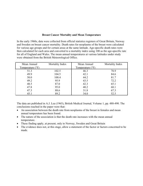
Breast Cancer Mortality and Mean Temperature
In the early 1960s, data were collected from official statistics registers of Great Britain, Norway
and Sweden on breast cancer mortality. Death rates for neoplasms of the breast were calculated
for various age groups and for certain areas at the same latitude. Age-specific death rates were
then calculated for each area and converted to a mortality index using 100 as the age-specific rate
for all of England and Wales. The mean annual temperatures at various latitudes under study
were obtained from the British Meteorological Office.
Mean Annual Mortality Index Mean Annual Mortality Index
Temperature (°F)
Temperature (°F)
51.3 102.5 46.3 78.9
49.9 104.5 42.1 84.6
50.0 100.4 44.2 81.7
49.2 95.9 43.5 72.2
48.5 87.0 42.3 65.1
47.8 95.0 40.2 68.1
47.3 88.6 31.8 67.3
45.1 89.2 34.0 52.5
The data are published in A.J. Lea (1965), British Medical Journal, Volume 1, pp. 488-490. The
conclusions reached in the paper were that:
• An association between the death rate from neoplasms of the breast in females and mean
annual temperature has been found.
• The nature of the association is that the death rate increases with the mean annual
temperature.
• These finding apply, at present, only to Norway, Sweden and Great Britain
• The evidence does not, at this stage, allow a statement of the factor or factors concerned to be
made.

Regression Analysis in R: Breast Cancer Data
> cancer attach(cancer)
> cancer
temp mortality
1 51.3 102.5
2 49.9 104.5
3 50.0 100.4
4 49.2 95.9
5 48.5 87.0
6 47.8 95.0
7 47.3 88.6
8 45.1 89.2
9 46.3 78.9
10 42.1 84.6
11 44.2 81.7
12 43.5 72.2
13 42.3 65.1
14 40.2 68.1
15 31.8 67.3
16 34.0 52.5
> plot(temp,mortality)
mortality
60 70 80 90 100
35 40 45 50
temp
2

egout summary(regout)
Call:
lm(formula = mortality ~ temp)
Residuals:
Min 1Q Median 3Q Max
-12.8358 -5.6319 0.4904 4.3981 14.1200
Coefficients:
Estimate Std. Error t value Pr(>|t|)
(Intercept) -21.7947 15.6719 -1.391 0.186
temp 2.3577 0.3489 6.758 9.2e-06 ***
---
Signif. codes: 0 '***' 0.001 '**' 0.01 '*' 0.05 '.' 0.1 ' ' 1
Residual standard error: 7.545 on 14 degrees of freedom
Multiple R-Squared: 0.7654, Adjusted R-squared: 0.7486
F-statistic: 45.67 on 1 and 14 DF, p-value: 9.202e-06
> anova(regout)
Analysis of Variance Table
Response: mortality
Df Sum Sq Mean Sq F value Pr(>F)
temp 1 2599.53 2599.53 45.669 9.202e-06 ***
Residuals 14 796.91 56.92
---
Signif. codes: 0 '***' 0.001 '**' 0.01 '*' 0.05 '.' 0.1 ' ' 1
> rescan plot(temp,rescan)
rescan
-10 -5 0 5 10 15
35 40 45 50
temp
3

newtemp tempred tempred
1 2 3 4 5 6 7 8
53.65153 56.00923 58.36692 60.72462 63.08231 65.44001 67.79770 70.15540
9 10 11 12 13 14 15 16
72.51309 74.87079 77.22848 79.58617 81.94387 84.30156 86.65926 89.01695
17 18 19 20
91.37465 93.73234 96.09004 98.44773
> predict(regout,newtemp,interval="confidence")
fit lwr upr
1 53.65153 43.39628 63.90679
2 56.00923 46.43702 65.58144
3 58.36692 49.46726 67.26659
4 60.72462 52.48444 68.96480
5 63.08231 55.48514 70.67948
6 65.44001 58.46482 72.41520
7 67.79770 61.41731 74.17809
8 70.15540 64.33428 75.97651
9 72.51309 67.20450 77.82169
10 74.87079 70.01313 79.72844
11 77.22848 72.74158 81.71538
12 79.58617 75.36863 83.80371
13 81.94387 77.87413 86.01361
14 84.30156 80.24474 88.35839
15 86.65926 82.47922 90.83929
16 89.01695 84.58893 93.44498
17 91.37465 86.59323 96.15606
18 93.73234 88.51350 98.95118
19 96.09004 90.36898 101.81110
20 98.44773 92.17520 104.72026
> predict(regout,newtemp,interval="prediction")
fit lwr upr
1 53.65153 34.49385 72.80922
2 56.00923 37.20833 74.81013
3 58.36692 39.89937 76.83448
4 60.72462 42.56567 78.88356
5 63.08231 45.20597 80.95866
6 65.44001 47.81900 83.06102
7 67.79770 50.40356 85.19184
8 70.15540 52.95853 87.35226
9 72.51309 55.48288 89.54330
10 74.87079 57.97571 91.76586
11 77.22848 60.43625 94.02071
12 79.58617 62.86390 96.30845
13 81.94387 65.25826 98.62948
14 84.30156 67.61910 100.98403
15 86.65926 69.94641 103.37211
16 89.01695 72.24036 105.79355
17 91.37465 74.50133 108.24796
18 93.73234 76.72990 110.73478
19 96.09004 78.92678 113.25329
20 98.44773 81.09287 115.80260
4