Estimation, Evaluation, and Selection of Actuarial Models

5.2. PROPORTIONAL HAZARDS MODELS 91
Exercise 92 (*) The duration of a strike follows a Cox proportional hazards model in which the
baseline distribution has an exponential distribution. The only variable used is the index of industrial
production. When the index has a value of 10, the mean duration of a strike is 0.2060 years. When
the index has a value of 25, the median duration is 0.0411 years. Determine the probability that a
strike will have a duration of more than one year if the index has a value of 5.
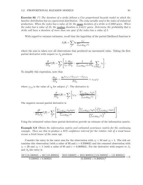
With regard to variance estimates, recall that the logarithm of the partial likelihood function is
l(β) = X j ∗
ln
c j ∗
P
i∈R(y j ) c i
where the sum is taken over all observations that produced an uncensored value. Taking the first
partial derivative with respect to β g produces
⎡
∂
l(β) = X ∂β g j ∗
To simplify this expression, note that
⎣ 1
c j ∗
∂c j ∗
∂β g
−
1
P
i∈R(y j ) c i
∂c j ∗
∂β g
= ∂eβ 1 z j ∗ 1+β 2 z j ∗ 2 +···+β p z j ∗ p
∂β g
∂
∂β g
X
i∈R(y j )
= z j ∗ gc j ∗
where z j ∗ g is the value of z g for subject j ∗ . The derivative is
∂
l(β) = X " P
i∈R(y
z j
∂β ∗ g −
j ) z #
igc i
P
g j ∗ i∈R(y j ) c .
i
The negative second partial derivative is
⎡
∂2
− l(β) = X ∂β h β g j ∗
⎢
⎣
P
i∈R(y j ) z igz ih c i
P
i∈R(y j ) c −
i
c i
⎤
⎦ .
³ ⎤
P P
i∈R(y j ) z igc i´³
i∈R(y j ) z ihc i´
³ P
i∈R(y j ) c i´2
Using the estimated values these partial derivatives provide an estimate of the information matrix.
Example 5.9 Obtain the information matrix and estimated covariance matrix for the continuing
example. Then use this to produce a 95% confidence interval for the relative risk of a wood house
versus a brick house of the same age.
Consider the entry in the outer sum for the observation with z 1 =50and z 2 =1. The risk set
contains this observation (with a value of 93 and c =0.330802) and the censored observation with
z 1 =20and z 2 =1(with a value of 95 and c =0.369924). For the derivative with respect to β 1
and β 2 the entry is
50(1)(0.330802) + 20(1)(0.369924) [50(0.330802) + 20(0.369924)][1(0.330802) + 1(0.369924)]
−
0.330802 + 0.369924
(0.330802 + 0.369924) 2 =0.
⎥
⎦ .