Estimation, Evaluation, and Selection of Actuarial Models

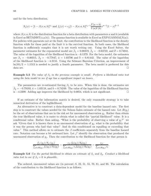
88 CHAPTER 5. MODELS WITH COVARIATES
and for the beta distribution,
S j (x) =[1− β(x; a, b)] c j
and f j (x) =c j [1 − β(x; a, b)] c Γ(a + b)
j−1
Γ(a)Γ(b) xa−1 (1 − x) b−1
where β(x; a, b) is the distribution function for a beta distribution with parameters a and b (available
in Excel as BETADIST(x,a,b)). The gamma function is available in Excel as EXP(GAMMALN(a)).
For policies with payments not at the limit, the contribution to the likelihood function is the density
function while for those paid at the limit it is the survival function. In both cases, the likelihood
function is sufficiently complex that it is not worth writing out. Using the Excel Solver, the
parameter estimates for the exponential model are ˆβ 1 =0.00319, ˆβ 2 = −0.63722, andˆθ =0.74041.
The value of the logarithm of the likelihood function is −6.1379. For the beta model, the estimates
are ˆβ 1 = −0.00315, ˆβ 2 = −0.77847, â =1.03706 and ˆb =0.81442. The value of the logarithm
of the likelihood function is −4.2155. Using the Schwarz Bayesian Criterion, an improvement of
ln(10)/2 =1.1513 is needed to justify a fourth parameter. The beta model is preferred for this
data set. ¤
Example 5.5 The value of β 1 in the previous example is small. Perform a likelihood ratio test
using the beta model to see if age has a significant impact on losses.
The parameters are re-estimated forcing β 1 to be zero. When this is done, the estimates are
ˆβ 2 = −0.79193, â =1.03118, andˆb =0.74249. The value of the logarithm of the likelihood function
is −4.2209. Adding age improves the likelihood by 0.0054, which is not significant. ¤
If an estimate of the information matrix is desired, the only reasonable strategy is to take
numerical derivatives of the loglikelihood.
An alternative is to construct a data-dependent model for the baseline hazard rate. The first
step is to construct the values needed for the Nelson-Åalen estimate of the hazard rate. Let R(y j )
be the set of observations that are in the risk set for uncensored observation y j . Rather than obtain
the true likelihood value, it is easier to obtain what is called the “partial likelihood” value. It is a
conditional value. Rather than asking, “What is the probability of observing a value of y j ?” we
ask “Given that it is known there is an uncensored observation of y j , what is the probability that
it was the person who had that value? And do this conditioned on equalling or exceeding that
value.” This method allows us to estimate the β coefficients separately from the baseline hazard
rate. Notation can become a bit awkward here. Let j ∗ identify the observation that produced the
uncensored observation of y j . Then the contribution to the likelihood function for that person is
f j ∗(y j )/S j ∗(y j )
P
i∈R(y j ) f i(y j )/S i (y j ) = c j ∗f 0 (y j )/S 0 (y j )
P
i∈R(y j ) c if 0 (y j )/S 0 (y j ) =
c j ∗
P
i∈R(y j ) c i
.
Example 5.6 Use the partial likelihood to obtain an estimate of β 1 and β 2 . Conduct a likelihood
ratiotesttoseeifβ 1 =0is plausible.
The ordered, uncensored values are (in percent) 8, 22, 51, 55, 70, 81, and 93. The calculation
of the contribution to the likelihood function is as follows.