Estimation, Evaluation, and Selection of Actuarial Models

82 CHAPTER 4. MODEL EVALUATION AND SELECTION
Aside from the issue of special cases, the likelihood ratio test has the same problem as the other
hypothesis tests in this Chapter. Were the sample size to double, the loglikelihoods would also
double, making it more likely that a model with a higher number of parameters will be selected.
This tends to defeat the parsimony principle. On the other hand, it could be argued that if we
possess a lot of data, we have the right to consider and fit more complex models. A method that
effects a compromise between these positions is the Schwarz Bayesian Criterion (“Estimating the
Dimension of a Model,” G. Schwarz, Annals of Mathematical Statistics, Vol. 6, pp. 461—464, 1978).
In that paper, he suggests that when ranking models a deduction of (r/2) ln n should be made from
the loglikelihood value where r is the number of estimated parameters and n is the sample size. 6
Thus, adding a parameter requires an increase of 0.5lnn in the loglikelihood. For larger sample
sizes, a greater increase is needed, but it is not proportional to the sample size itself.
Example 4.18 For the continuing example in this Chapter, choose between the exponential and
Weibull models for the data.
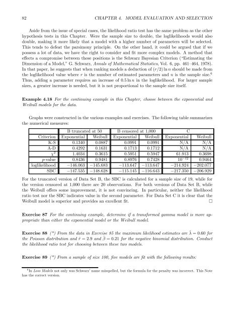
Graphs were constructed in the various examples and exercises. The following table summarizes
the numerical measures:
B truncated at 50 B censored at 1,000 C
Criterion Exponential Weibull Exponential Weibull Exponential Weibull
K-S 0.1340 0.0887 0.0991 0.0991 N/A N/A
A-D 0.4292 0.1631 0.1713 0.1712 N/A N/A
χ 2 1.4034 0.3615 0.5951 0.5947 61.913 0.3698
p-value 0.8436 0.9481 0.8976 0.7428 10 −12 0.9464
loglikelihood −146.063 −145.683 −113.647 −113.647 −214.924 −202.077
SBC −147.535 −148.628 −115.145 −116.643 −217.350 −206.929
For the truncated version of Data Set B, the SBC is calculated for a sample size of 19, while for
the version censored at 1,000 there are 20 observations. For both versions of Data Set B, while
the Weibull offers some improvement, it is not convincing. In particular, neither the likelihood
ratio test nor the SBC indicates value in the second parameter. For Data Set C it is clear that the
Weibull model is superior and provides an excellent fit. ¤
Exercise 87 For the continuing example, determine if a transformed gamma model is more appropriate
than either the exponential model or the Weibull model.
Exercise 88 (*) From the data in Exercise 85 the maximum likelihood estimates are ˆλ =0.60 for
the Poisson distribution and ˆr =2.9 and ˆβ =0.21 for the negative binomial distribution. Conduct
the likelihood ratio test for choosing between these two models.
Exercise 89 (*) From a sample of size 100, five models are fit with the following results:
6 In Loss Models not only was Schwarz’ name misspelled, but the formula for the penalty was incorrect. This Note
has the correct version.