Estimation, Evaluation, and Selection of Actuarial Models

66 CHAPTER 4. MODEL EVALUATION AND SELECTION
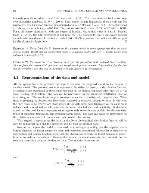
but only over those values α and θ for which αθ =1, 200. That means α canbefreetorange
over all positive numbers, but θ =1, 200/α. Thus, under the null hypothesis, there is only one free
parameter. The likelihood function is maximized at ˆα =0.54955 and ˆθ =2, 183.6. The loglikelihood
at this maximum is ln L 0 = −162.466. The test statistic is T =2(−162.293 + 162.466) = 0.346.
For a chi-square distribution with one degree of freedom, the critical value is 3.8415. Because
0.346 < 3.8415, the null hypothesis is not rejected. The probability that a chi-square random
variable with one degree of freedom exceeds 0.346 is 0.556, a p-value that indicates little support
for the alternative hypothesis. ¤
Exercise 73 Using Data Set B, determine if a gamma model is more appropriate than an exponential
model. Recall that an exponential model is a gamma model with α =1.Usefulvalueswere
obtained in Example 2.32.
Exercise 74 Use Data Set C to choose a model for the population that produced those numbers.
Choose from the exponential, gamma, and transformed gamma models. Information for the first
two distributions was obtained in Example 2.33 and Exercise 28 respectively.
4.3 Representations of the data and model
All the approaches to be presented attempt to compare the proposed model to the data or to
another model. The proposed model is represented by either its density or distribution function,
or perhaps some functional of these quantities such as the limited expected value function or the
mean residual life function. The data can be represented by the empirical distribution function
or a histogram. The graphs are easy to construct when there is individual, complete data. When
there is grouping, or observations have been truncated or censored, difficulties arise. In this Note
the only cases to be covered are those where all the data have been truncated at the same value
(which could be zero) and are all censored at the same value (which could be infinity). It should be
noted that the need for such representations applies only to continuous models. For discrete data,
issues of censoring, truncation, and grouping rarely apply. The data can easily be represented by
the relative or cumulative frequencies at each possible observation.
With regard to representing the data, in this Note the empirical distribution function will be
used for individual data and the histogram will be used for grouped data.
In order to compare the model to truncated data, we begin by noting that the empirical distribution
begins at the lowest truncation point and represents conditional values (that is, they are the
distribution and density function given that the observation exceeds the lowest truncation point).
In order to make a comparison to the empirical values, the model must also be truncated. Let the
common truncation point in the data set be t. The modified functions are
(
0, x < t
F ∗ (x) = F (x)−F (t)
1−F (t)
, x ≥ t
and
(
0, x < t
f ∗ (x) = f(x)
1−F (t) , x ≥ t.