Estimation, Evaluation, and Selection of Actuarial Models

More documents

Recommendations

Info

62 CHAPTER 4. MODEL EVALUATION AND SELECTION This Chapter begins with a review of hypothesis testing, mostly because it is no longer directly covered on prior actuarial examinations. The remaining sections cover a variety of evaluation and selection tools. Each tool has its own strengths and weaknesses and it is possible for different tools to lead to different models. This makes modeling as much art as science. At times, in real-world applications, the model’s purpose may lead the analyst to favor one tool over another. 4.2 A review of hypothesis tests The Neyman-Pearson approach to hypothesis testing is covered in detail in most mathematical statistics texts. This review will be fairly straightforward and will not address philosophical issues or consider alternative approaches. A hypothesis test begins with two hypotheses, one called the null and one called the alternative. The traditional notation is H 0 for the null hypothesis and H 1 for the alternative hypothesis. The two hypotheses are not treated symmetrically. Reversing them may alter the results. To illustrate this process, a simple example will be used. Example 4.1 Your company has been basing its premiums on an assumption that the average claim is 1,200. You want to raise the premium and a regulator has demanded that you provide evidence that the average now exceeds 1,200. To provide such evidence, the numbers in Data Set B have been obtained. What are the hypotheses for this problem? Let µ be the population mean. One hypothesis (the one you claim is true) is that µ>1, 200. Because hypothesis tests must present an either/or situation, the other hypothesis must be µ ≤ 1, 200. The only remaining task is to decide which of them is the null hypothesis. Whenever the universe of continuous possibilities is divided in two there is likely to be a boundary that needs to be assigned to one hypothesis or the other. The hypothesis that includes the boundary must be the null hypothesis. Therefore, the problem can be succinctly stated as: H 0 : µ ≤ 1, 200 H 1 : µ>1, 200. ¤ The decision is made by calculating a quantity called a test statistic. It is a function of the observations and is treated as a random variable. That is, in designing the test procedure we are concerned with the samples that might have been obtained and not with the particular sample that was obtained. The test specification is completed by constructing a rejection region. Itisa subset of the possible values of the test statistic. If the value of the test statistic for the observed sample is in the rejection region, the null hypothesis is rejected and the alternative hypothesis is announced as the result that is supported by the data. Otherwise, the null hypothesis is not rejected (more on this later). The boundaries of the rejection region (other than plus or minus infinity) are called the critical values. Example 4.2 For the continuing example, complete the test using the test statistic and rejection region that is promoted in most statistics books. Assume that the population that produced Data Set B has a normal distribution with standard deviation 3,435.
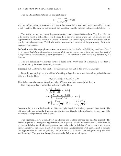
4.2. A REVIEW OF HYPOTHESIS TESTS 63 The traditional test statistic for this problem is ¯x − 1, 200 z = 3, 435/ √ 20 =0.292 and the null hypothesis is rejected if z>1.645. Because 0.292 is less than 1.645, the null hypothesis is not rejected. The data do not support the assertion that the average claim exceeds 1,200. ¤ The test in the previous example was constructed to meet certain objectives. The first objective is to control what is called the Type I error. It is the error made when the test rejects the null hypothesis in a situation where it happens to be true. In the example, the null hypothesis can be true in more than one way. This leads to the most common measure of the propensity of a test to make a Type I error. Definition 4.3 The significance level of a hypothesis test is the probability of making a Type I error, given that the null hypothesis is true. If it can be true in more than one way, the level of significance is the maximum of such probabilities. The significance level is usually denoted by the letter α. This is a conservative definition in that it looks at the worst case. It is typically a case that is on the boundary between the two hypotheses. Example 4.4 Determine the level of significance for the test in the previous example. Begin by computing the probability of making a Type I error when the null hypothesis is true with µ =1, 200. Then, Pr(Z >1.645|µ =1, 200) = 0.05. That is because the assumptions imply that Z has a standard normal distribution. Now suppose µ has a value that is below 1,200. Then µ ¯X − 1, 200 Pr 3, 435/ √ 20 > 1.645 µ ¯X − µ + µ − 1, 200 =Pr 3, 435/ √ > 1.645 20 µ ¯X − µ =Pr 3.435/ √ µ − 1, 200 > 1.645 − 20 3.435/ √ . 20 Because µ is known to be less than 1,200, the right hand side is always greater than 1.645. The left hand side has a standard normal distribution and therefore the probability is less than 0.05. Therefore the significance level is 0.05. ¤ The significance level is usually set in advance and is often between one and ten percent. The second objective is to keep the Type II error (not rejecting the null hypothesis when the alternative is true) probability small. Generally, attempts to reduce the probability of one type of error increase the probability of the other. The best we can do once the significance level has been set is to make the Type II error as small as possible, though there is no assurance that the probability will be a small number. The best test is one that meets the following requirement.
Page 1:
Estimation, Evaluation, and Selecti
Page 4 and 5:
iv CONTENTS 4.5.2 Anderson-Darlingt
Page 6 and 7:
2 CHAPTER 1. INTRODUCTION Exercises
Page 8 and 9:
4 CHAPTER 2. MODEL ESTIMATION Throu
Page 10 and 11:
6 CHAPTER 2. MODEL ESTIMATION 2.2 E
Page 12 and 13:
8 CHAPTER 2. MODEL ESTIMATION and t
Page 14 and 15:
10 CHAPTER 2. MODEL ESTIMATION of t
Page 16 and 17: 12 CHAPTER 2. MODEL ESTIMATION Exer
Page 18 and 19: 14 CHAPTER 2. MODEL ESTIMATION i d
Page 20 and 21: 16 CHAPTER 2. MODEL ESTIMATION 8. C
Page 24 and 25: 20 CHAPTER 2. MODEL ESTIMATION In e
Page 26 and 27: 22 CHAPTER 2. MODEL ESTIMATION Exam
Page 28 and 29: 24 CHAPTER 2. MODEL ESTIMATION That
Page 30 and 31: 26 CHAPTER 2. MODEL ESTIMATION Unle
Page 32 and 33: 28 CHAPTER 2. MODEL ESTIMATION like
Page 34 and 35: 30 CHAPTER 2. MODEL ESTIMATION For
Page 36 and 37: 32 CHAPTER 2. MODEL ESTIMATION like
Page 38 and 39: 34 CHAPTER 2. MODEL ESTIMATION wher
Page 42 and 43: 38 CHAPTER 3. SAMPLING PROPERTIES O
Page 68 and 69: 64 CHAPTER 4. MODEL EVALUATION AND
Page 90 and 91: 86 CHAPTER 5. MODELS WITH COVARIATE
Page 100 and 101: 96 APPENDIX A. SOLUTIONS TO EXERCIS
Page 102 and 103: 98 APPENDIX A. SOLUTIONS TO EXERCIS
Page 104 and 105: 100 APPENDIX A. SOLUTIONS TO EXERCI
Page 116 and 117:
112 APPENDIX A. SOLUTIONS TO EXERCI
Page 118 and 119:
Page 120 and 121:
Page 122 and 123:
Page 124 and 125:
Page 126 and 127:
Page 128 and 129:
Page 130 and 131:
Page 132 and 133:
Page 134 and 135:
Page 136 and 137:
132 APPENDIX B. USING MICROSOFT EXC
Page 138 and 139:
Page 140 and 141:
Page 142:
show all

Estimation, Evaluation, and Selection of Actuarial Models

Create successful ePaper yourself

Delete template?

Save as template?