Estimation, Evaluation, and Selection of Actuarial Models

24 CHAPTER 2. MODEL ESTIMATION
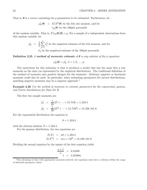
That is, θ is a vector containing the p parameters to be estimated. Furthermore, let
µ 0 k (θ) = E(Xk |θ) be the kth raw moment, and let
π g (θ) be the 100gth percentile
of the random variable. That is, F [π g (θ)|θ] =g. Forasampleofn independent observations from
this random variable, let
ˆµ 0 k = 1 nX
x k j be the empirical estimate of the kth moment, and let
n
j=1
ˆπ g be the empirical estimate of the 100gth percentile.
Definition 2.25 A method of moments estimate of θ is any solution of the p equations
µ 0 k (θ) =ˆµ0 k , k =1, 2,...,p.
The motivation for this estimator is that it produces a model that has the same first p raw
moments as the data (as represented by the empirical distribution). The traditional definition of
the method of moments uses positive integers for the moments. Arbitrary negative or fractional
moments could also be used. In particular, when estimating parameters for inverse distributions,
matching negative moments may be a superior approach. 4
Example 2.26 Use the method of moments to estimate parameters for the exponential, gamma,
and Pareto distributions for Data Set B.
The first two sample moments are
For the exponential distribution the equation is
ˆµ 0 1 = 1 (27 + ···+15, 743) = 1, 424.4
20
ˆµ 0 2 = 1 20 (272 + ···+15, 743 2 )=13, 238, 441.9.
θ =1, 424.4
with the obvious solution, ˆθ =1, 424.4.
For the gamma distribution, the two equations are
E(X) = αθ =1, 424.4
E(X 2 ) = α(α +1)θ 2 =13, 238, 441.9.
Dividing the second equation by the square of the first equation yields
α +1
α
= 6.52489
1 = 5.52489α
4 One advantage is that with appropriate moments selected, the equations must have a solution within the range
of allowable parameter values.