Estimation, Evaluation, and Selection of Actuarial Models
Estimation, Evaluation, and Selection of Actuarial Models Estimation, Evaluation, and Selection of Actuarial Models
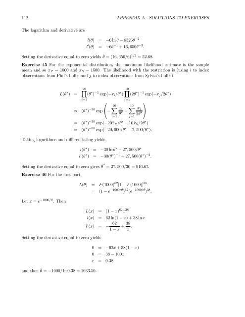
112 APPENDIX A. SOLUTIONS TO EXERCISES The logarithm and derivative are l(θ) = −6lnθ − 8325θ −2 l 0 (θ) = −6θ −1 +16, 650θ −3 . Setting the derivative equal to zero yields ˆθ =(16, 650/6) 1/2 =52.68. Exercise 45 For the exponential distribution, the maximum likelihood estimate is the sample mean and so ¯x P = 1000 and ¯x S =1500. The likelihood with the restriction is (using i to index observations from Phil’s bulbs and j to index observations from Sylvia’s bulbs) L(θ ∗ ) = ∝ 20Y i=1 (θ ∗ ) −1 exp(−x i /θ ∗ ) ⎛ (θ ∗ ) −30 exp ⎝− Taking logarithms and differentiating yields 20X i=1 10Y j=1 (2θ ∗ ) −1 exp(−x j /2θ ∗ ) ⎞ x i 10X θ ∗ − x j ⎠ 2θ ∗ j=1 = (θ ∗ ) −30 exp(−20¯x P /θ ∗ − 10¯x S /2θ ∗ ) = (θ ∗ ) −30 exp(−20, 000/θ ∗ − 7, 500/θ ∗ ). l(θ ∗ ) = −30 ln θ ∗ − 27, 500/θ ∗ l 0 (θ ∗ ) = −30(θ ∗ ) −1 +27, 500(θ ∗ ) −2 . Setting the derivative equal to zero gives ˆθ ∗ =27, 500/30 = 916.67. Exercise 46 For the first part, Let x = e −1000/θ .Then L(θ) = F (1000) 62 [1 − F (1000)] 38 = (1− e −1000/θ ) 62 (e −1000/θ ) 38 . L(x) = (1− x) 62 x 38 l(x) = 62ln(1− x)+38lnx l 0 (x) = − 62 1 − x + 38 x . Setting the derivative equal to zero yields and then ˆθ = −1000/ ln 0.38 = 1033.50. 0 = −62x + 38(1 − x) 0 = 38− 100x x = 0.38
113 With additional information ⎡ ⎤ ⎛ ⎞ 62Y Y62 L(θ) = ⎣ f(x j ) ⎦ [1 − F (1000)] 38 = ⎝ θ −1 e −x j/θ⎠ e −38,000/θ j=1 j=1 = θ −62 e −28,140/θ e −38,000/θ = θ −62 e −66,140/θ l(θ) = −62 ln θ − 66, 140/θ l 0 (θ) = −62/θ +66, 140/θ 2 =0 0 = −62θ +66, 140 ˆθ = 66, 140/62 = 1066.77. Exercise 47 The density function is f(x) =0.5x −0.5 θ −0.5 e −(x/θ)0.5 . The likelihood function and subsequent calculations are à Y10 L(θ) = θ −0.5 e −x0.5 j θ −0.5 ∝ θ −5 exp −θ −0.5 P 10 j=1 0.5x −0.5 j l(θ) = −5lnθ − 488.97θ −0.5 j=1 x 0.5 j ! = θ −5 exp(−488.97θ −0.5 ) l 0 (θ) = −5θ −1 +244.485θ −1.5 =0 0 = −5θ 0.5 +244.485 and so ˆθ = (244.485/5) 2 = 2391. Exercise 48 Each observation has a uniquely determined conditional probability. The contribution to the loglikelihood is given in the following table: Observation Probability Loglikelihood Pr(N=1) 1997-1 Pr(N=1)+Pr(N=2) = (1−p)p (1−p)p+(1−p)p = 1 2 1+p −3ln(1+p) Pr(N=2) 1997-2 Pr(N=1)+Pr(N=2) = (1−p)p 2 (1−p)p+(1−p)p = p 2 1+p ln p − ln(1 + p) Pr(N=0) 1998-0 Pr(N=0)+Pr(N=1) = (1−p) (1−p)+(1−p)p = 1+p 1 −5ln(1+p) Pr(N=1) 1998-1 Pr(N=0)+Pr(N=1) = (1−p)p (1−p)+(1−p)p = p 1+p 2lnp − 2ln(1+p) Pr(N=0) 1999-0 Pr(N=0) =1 0 The total is l(p) =3lnp − 11 ln(1 + p). Setting the derivative equal to zero gives 0=l 0 (p) = 3p −1 − 11(1 + p) −1 and the solution is ˆp =3/8. Exercise 49 When three observations are taken without replacement there are only four possible results. They are 1,3,5; 1,3,9; 1,5,9; and 3,5,9. The four sample means are 9/3, 13/3, 15/3, and 17/3. The expected value (each has probability 1/4) is 54/12 or 4.5, which equals the population mean. The four sample medians are 3, 3, 5, and 5. The expected value is 4 and so the median is biased. Exercise 50 · ¸ E( ¯X) 1 = E n (X 1 + ···+ X n ) = 1 n [E(X 1)+···+ E(X n )] = 1 (µ + ···+ µ) =µ. n
- Page 66 and 67: 62 CHAPTER 4. MODEL EVALUATION AND
- Page 68 and 69: 64 CHAPTER 4. MODEL EVALUATION AND
- Page 70 and 71: 66 CHAPTER 4. MODEL EVALUATION AND
- Page 72 and 73: 68 CHAPTER 4. MODEL EVALUATION AND
- Page 74 and 75: 70 CHAPTER 4. MODEL EVALUATION AND
- Page 76 and 77: 72 CHAPTER 4. MODEL EVALUATION AND
- Page 78 and 79: 74 CHAPTER 4. MODEL EVALUATION AND
- Page 80 and 81: 76 CHAPTER 4. MODEL EVALUATION AND
- Page 82 and 83: 78 CHAPTER 4. MODEL EVALUATION AND
- Page 84 and 85: 80 CHAPTER 4. MODEL EVALUATION AND
- Page 86 and 87: 82 CHAPTER 4. MODEL EVALUATION AND
- Page 88 and 89: 84 CHAPTER 4. MODEL EVALUATION AND
- Page 90 and 91: 86 CHAPTER 5. MODELS WITH COVARIATE
- Page 92 and 93: 88 CHAPTER 5. MODELS WITH COVARIATE
- Page 94 and 95: 90 CHAPTER 5. MODELS WITH COVARIATE
- Page 96 and 97: 92 CHAPTER 5. MODELS WITH COVARIATE
- Page 98 and 99: 94 CHAPTER 5. MODELS WITH COVARIATE
- Page 100 and 101: 96 APPENDIX A. SOLUTIONS TO EXERCIS
- Page 102 and 103: 98 APPENDIX A. SOLUTIONS TO EXERCIS
- Page 104 and 105: 100 APPENDIX A. SOLUTIONS TO EXERCI
- Page 106 and 107: 102 APPENDIX A. SOLUTIONS TO EXERCI
- Page 108 and 109: 104 APPENDIX A. SOLUTIONS TO EXERCI
- Page 110 and 111: 106 APPENDIX A. SOLUTIONS TO EXERCI
- Page 112 and 113: 108 APPENDIX A. SOLUTIONS TO EXERCI
- Page 114 and 115: 110 APPENDIX A. SOLUTIONS TO EXERCI
- Page 118 and 119: 114 APPENDIX A. SOLUTIONS TO EXERCI
- Page 120 and 121: 116 APPENDIX A. SOLUTIONS TO EXERCI
- Page 122 and 123: 118 APPENDIX A. SOLUTIONS TO EXERCI
- Page 124 and 125: 120 APPENDIX A. SOLUTIONS TO EXERCI
- Page 126 and 127: 122 APPENDIX A. SOLUTIONS TO EXERCI
- Page 128 and 129: 124 APPENDIX A. SOLUTIONS TO EXERCI
- Page 130 and 131: 126 APPENDIX A. SOLUTIONS TO EXERCI
- Page 132 and 133: 128 APPENDIX A. SOLUTIONS TO EXERCI
- Page 134 and 135: 130 APPENDIX A. SOLUTIONS TO EXERCI
- Page 136 and 137: 132 APPENDIX B. USING MICROSOFT EXC
- Page 138 and 139: 134 APPENDIX B. USING MICROSOFT EXC
- Page 140 and 141: 136 APPENDIX B. USING MICROSOFT EXC
- Page 142: 138 APPENDIX B. USING MICROSOFT EXC
112 APPENDIX A. SOLUTIONS TO EXERCISES<br />
The logarithm <strong>and</strong> derivative are<br />
l(θ) = −6lnθ − 8325θ −2<br />
l 0 (θ) = −6θ −1 +16, 650θ −3 .<br />
Setting the derivative equal to zero yields ˆθ =(16, 650/6) 1/2 =52.68.<br />
Exercise 45 For the exponential distribution, the maximum likelihood estimate is the sample<br />
mean <strong>and</strong> so ¯x P = 1000 <strong>and</strong> ¯x S =1500. The likelihood with the restriction is (using i to index<br />
observations from Phil’s bulbs <strong>and</strong> j to index observations from Sylvia’s bulbs)<br />
L(θ ∗ ) =<br />
∝<br />
20Y<br />
i=1<br />
(θ ∗ ) −1 exp(−x i /θ ∗ )<br />
⎛<br />
(θ ∗ ) −30 exp ⎝−<br />
Taking logarithms <strong>and</strong> differentiating yields<br />
20X<br />
i=1<br />
10Y<br />
j=1<br />
(2θ ∗ ) −1 exp(−x j /2θ ∗ )<br />
⎞<br />
x i<br />
10X<br />
θ ∗ − x j<br />
⎠<br />
2θ ∗<br />
j=1<br />
= (θ ∗ ) −30 exp(−20¯x P /θ ∗ − 10¯x S /2θ ∗ )<br />
= (θ ∗ ) −30 exp(−20, 000/θ ∗ − 7, 500/θ ∗ ).<br />
l(θ ∗ ) = −30 ln θ ∗ − 27, 500/θ ∗<br />
l 0 (θ ∗ ) = −30(θ ∗ ) −1 +27, 500(θ ∗ ) −2 .<br />
Setting the derivative equal to zero gives ˆθ ∗ =27, 500/30 = 916.67.<br />
Exercise 46 For the first part,<br />
Let x = e −1000/θ .Then<br />
L(θ) = F (1000) 62 [1 − F (1000)] 38<br />
= (1− e −1000/θ ) 62 (e −1000/θ ) 38 .<br />
L(x) = (1− x) 62 x 38<br />
l(x) = 62ln(1− x)+38lnx<br />
l 0 (x) = − 62<br />
1 − x + 38 x .<br />
Setting the derivative equal to zero yields<br />
<strong>and</strong> then ˆθ = −1000/ ln 0.38 = 1033.50.<br />
0 = −62x + 38(1 − x)<br />
0 = 38− 100x<br />
x = 0.38


