Smoothing methods

Smoothing methods
Marzena Narodzonek-Karpowska
Prof. Dr. W. Toporowski
Institut für Marketing & Handel
Abteilung Handel

What Is Forecasting?
• Process of predicting a future event
• Underlying basis of all business decisions
You’ll never get it right. But, you can always get it less
wrong.

Realities of Forecasting
• Forecasts are seldom perfect
• Most forecasting methods assume that there is some
underlying stability in the system and future will be like
the past (causal factors will be the same).
• Accuracy decreases with length of forecast

Forecasting Methods
Qualitative Methods are subjective in nature since they rely
on human judgment and opinion.
• Used when situation is vague & little data exist
– New products
– New technology
• Involve intuition, experience
Quantitative Methods use mathematical or simulation
models based on historical demand or relationships
between variables.
• Used when situation is ‘stable’ & historical data exist
– Existing products
– Current technology
• Involve mathematical techniques

Forecasting Methods
Forecasting
Methods
Quantitative
Qualitative
Causal
Time Series
Smoothing
Trend
Projection
Trend Projection
Adjusted for
Seasonal Influence

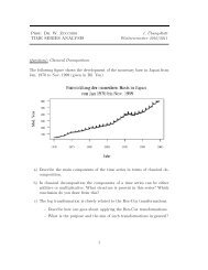
What is a Time Series?
By reviewing historical data over time, we can better understand
the pattern of past behavior of a variable and better predict the
future behavior.
• Set of evenly spaced numerical data
– Obtained by observing response variable at regular time
periods
• Forecast based only on past values
– Assumes that factors influencing past, present, & future
will continue
• Example
– Year: 2002 2003 2004 2005 2006
– Sales: 78.7 63.5 89.7 93.2 92.1

Time Series Forecasting
Time
Series
Smoothing
Methods
No
Trend?
Yes
Trend
Models
Moving
Average
Exponential
Smoothing
Linear
Quadratic
Exponential
Auto-
Regressive

Components of a Time Series
• The pattern or behavior of the data in a time series has
several components.
Trend
Cyclical
Seasonal
Irregular

Trend Component
• The trend component accounts for the gradual shifting of
the time series to relatively higher or lower values over a
long period of time.
• Trend is usually the result of long-term factors such as
changes in the population, demographics, technology, or
consumer preferences
Sales
Upward trend
Time

Cyclical Component
• Any regular pattern of sequences of values above and below
the trend line lasting more than one year can be attributed to
the cyclical component.
• Usually, this component is due to multiyear cyclical
movements in the economy.
Sales
1 Cycle
Year

Seasonal Component
• The seasonal component accounts for regular patterns of
variability within certain time periods, such as a year.
• The variability does not always correspond with the
seasons of the year (i.e. winter, spring, summer, fall).
• There can be, for example, within-week week or within-day
“seasonal” behavior.
Sales
Winter
Summer
Spring
Fall
Time (Quarterly)

Irregular Component
• The irregular component is caused by short-term,
term,
unanticipated and non-recurring factors that affect the values
of the time series.
• This component is the residual, or “catch-all,” all,” factor that
accounts for unexpected data values.
• It is unpredictable.

Components of Time Series Data
Trend
Seasonal
Cyclical
Irregular

Components of Time Series Data
Irregular
fluctuations
Cyclical
Trend
Seasonal
1 2 3 4 5 6 7 8 9 10 11 12 13
Year

Smoothing Methods
• In cases in which the time series is fairly stable and has no
significant trend, seasonal, or cyclical effects, one can use
smoothing methods to average out the irregular component
of the time series.
• Common smoothing methods are:
Moving Averages
Weighted Moving Averages
Centered Moving Average
Exponential Smoothing

Moving Averages Method
The moving averages method consists of computing an average
of the most recent n data values for the series and using this
average for forecasting the value of the time series for the next
period.
Moving averages are useful if one can assume item to be forecast
will stay fairly steady over time.
Series of arithmetic means - used only for smoothing, provides
overall impression of data over time
Moving Average =
∑
(most recent ndata values)
n

Moving Averages
Let us forecast sales for 2007 using a 3-period moving
average.
2002 4
2003 6
2004 5
2005 3
2006 7
2007 ?

Time
Moving Averages
Response
Yi
Moving
Total
(n=3)
Moving
Average
(n=3)
1995 2002 4 NA NA
1996 6 NA NA
1997 2004 5 NA NA
1998 2005 3 4+6+5=15 15/3=5.0
1999 2006 7 6+5+3=14 14/3=4.7
2000 2007 NA 5+3+7=15 15/3=5.0
0032003

Sales
8
6
4
Moving Averages Graph
Actual
Forecast
2
95 96 97 98 99 00
Year

Moving Averages Graph
Actual
Large n
Demand
Small n
Time

Centered Moving Averages
Method
The centered moving average method consists of
computing an average of n periods' data and associating it
with the midpoint of the periods. For example, the average
for periods 5, 6, and 7 is associated with period 6. This
methodology is useful in the process of computing season
indexes.
5 10
6 13 10+13+11: 3= 11.33
7 11

Weighted Moving Averages
• Used when trend is present
– Older data usually less important
• The more recent observations are typically
given more weight than older observations
• Weights based on intuition
– Often lay between 0 & 1, & sum to 1.0
WMA =
Σ(Weight for period n) (Value(
in period n)
ΣWeights

2x 12

Weighted Moving Average Graph
Actual
Small weight on
recent data
Demand
Large weight on
recent data
Time

Disadvantages of M.A. Methods
• Increasing n makes
forecast less sensitive to
changes
• Do not forecast trends
well
• Require sufficient
historical data

Responsiveness of M.A. Methods
The problem with M.A. Methods :
• Forecast lags with increasing demand
• Forecast leads with decreasing demand

Actual Demand, Moving Average,
Sales Demand
35
30
25
20
15
10
5
0
Weighted Moving Average
Actual sales
Jan
Feb
Mar
Apr
May
Jun
Weighted moving average
Moving average
Jul
Month
Aug
Sep
Oct
Nov
Dec
All forecasting methods lag ahead of or behind actual demand

M.A. versus Exponential
Smoothing
• Moving averages and weighted moving averages are
effective in smoothing out sudden fluctuations in demand
pattern in order to provide stable estimates.
• Requires maintaining extensive records of past data.
• Exponential smoothing requires little record keeping of
past data.
• Form of weighted moving average
– Weights decline exponentially
– Most recent data weighted most
• Requires smoothing constant (α)(
– Ranges from 0 to 1
– Subjectively chosen

Forecasting Using Smoothing Methods
Exponential
Smoothing
Methods
Single
Exponential
Smoothing
Double
(Holt’s)
Exponential
Smoothing
Triple
(Winter’s)
Exponential
Smoothing

Exponential Smoothing Methods
• Single Exponential Smoothing
– Similar to single MA
• Double (Holt’s) Exponential Smoothing
– Similar to double MA
– Estimates trend
• Triple (Winter’s) Exponential Smoothing
– Estimates trend and seasonality

Exponential Smoothing Model
• Single exponential smoothing model
F
t+
1
=
F
t
+ α(y
t
−
F )
t
or:
F
t+
1
= αy
t
+
(1−
α)
F
t
where:
F t+1
t+1 = forecast value for period t + 1
y t = actual value for period t
F t = forecast value for period t
α = alpha (smoothing constant)

Single Exponential Smoothing
• A weighted moving average
• Weights decline exponentially, most recent observation
weighted most
• The weighting factor is α
– Subjectively chosen
– Range from 0 to 1
– Smaller α gives more smoothing, larger α gives less
smoothing
• The weight is:
– Close to 0 for smoothing out unwanted cyclical and
irregular components
– Close to 1 for forecasting

Responsiveness to Different Values of α
3000
2500
2000
1500
1000
Actual demand
alpha = 0.1
alpha = 0.5
alpha = 0.9
1 2 3 4 5 6 7 8 9 10 11 12

Exponential Smoothing Example
• Suppose we use weight α = 0.2
Quarter
(t)
1
2
3
4
5
6
7
8
9
10
etc…
Sales
(y t
)
23
40
25
27
32
48
33
37
37
50
etc…
Forecast
from prior
period
NA
23
26.4
26.12
26.296
27.437
31.549
31.840
32.872
33.697
etc…
Forecast for next period
(F t+1
)
23
(.2)(40)+(.8)(23)=26.4
(.2)(25)+(.8)(26.4)=26.12
(.2)(27)+(.8)(26.12)=26.296
(.2)(32)+(.8)(26.296)=27.437
(.2)(48)+(.8)(27.437)=31.549
(.2)(48)+(.8)(31.549)=31.840
(.2)(33)+(.8)(31.840)=32.872
(.2)(37)+(.8)(32.872)=33.697
(.2)(50)+(.8)(33.697)=36.958
etc…
F
t+
1
= αy
F 1
= y 1
since no
prior
informatio
n exists
t
+ (1− α)F
t

Sales vs. Smoothed Sales
• Seasonal
fluctuations have
been smoothed
• The smoothed
value in this case
is generally a little
low, since the
trend is upward
sloping and the
weighting factor is
only 0.2
Sales
60
50
40
30
20
10
0
1 2 3 4 5 6 7 8 9 10
Quarter
Sales
Smoothed

Double Exponential Smoothing
• Double exponential smoothing is sometimes called
exponential smoothing with trend
• If trend exists, single exponential smoothing may need
adjustment
• There is a need to add a second smoothing constant to
account for trend

Double Exponential Smoothing
Model
Ct
= αy
t
+ (1− α)(Ct− 1
+ Tt
−1)
T
t
= β(C
F = C +
t+
1
y t = actual value in time t
t
t
−
T
t
C
t−1
α = constant-process smoothing constant
β = trend-smoothing constant
C t = smoothed constant-process value for period t
T t = smoothed trend value for period t
F t+1 = forecast value for period t + 1
t = current time period
)
+ (1−
β)
T
t−1

Double Exponential Smoothing
•Double Double exponential smoothing is generally done by
computer
•One One uses larger smoothing constants α and β when less
smoothing is desired
•One One uses smaller smoothing constants α and β when more
smoothing is desired

Exponential Smoothing Method
You want to forecast sales for 2007 using exponential
smoothing (α(
= 0.10). The 2001 forecast was 175.
2002 180
2003 168
2004 159
2005 175
2006 190

Exponential Smoothing Method
Time
Actual
F t = F t-1 + α (A t-1 - F t-1 )
Forecast,
(α =0.10)
2002 180 175.00 (Given)
2003 168 175.00 + .10(180 - 175.00) = 175.50
2004 159 175.50 + .10(168 - 175.50) = 174.75
2005 175 174.75 + .10(159 - 174.75) = 173.18
2006 190 173.18 + .10(175 - 173.18) = 173.36
2007 NA 173.36 + .10(190 - 173.36) = 175.02
F t

Exponential Smoothing Graph
Sales
190
180
170
160
150
140
Actual
Forecast
Year
02 03 04 05 06 07

Exponential Smoothing Graph
Actual
Small α
Demand
Large α
Time

Comparing Smoothing Techniques
• Let us determine the smoothing technique that is best for
forecasting these sales data : A two period moving
average, a three period moving average, exponential
smoothing (α=0.1),(
or exponential smoothing (α=0.2)(
Week
Sales
Week
Sales
1 110 6 120
2 115 7 130
3 125 8 115
4 120 9 110
5 125 10 130

Measures of Forecast Accuracy
Mean Squared Error (MSE)
The average of the squared forecast errors for the historical
data is calculated. The forecasting method or parameter(s)
which minimize this mean squared error is then selected.
Mean Absolute Deviation (MAD)
The mean of the absolute values of all forecast errors is
calculated, and the forecasting method or parameter(s) which
minimize this measure is selected. The mean absolute
deviation measure is less sensitive to individual large forecast
errors than the mean squared error measure.
You may choose either of the above criteria for evaluating the
accuracy of a method (or parameter).

2 period moving average
Sales n=2 Error
Week (t ) Y t F t (Y t - F t ) (Y t - F t ) 2
1 110
2 115 #NV
3 125 112,5 12,5 156,25
4 120 120 0 0
5 125 122,5 2,5 6,25
6 120 122,5 -2,5 6,25
7 130 122,5 7,5 56,25
8 115 125 -10 100
9 110 122,5 -12,5 156,25
10 130 112,5 17,5 306,25
11 120
MSE 98,4375

3 period moving average
Sales n=3 Error
Week (t ) Y t F t (Y t - F t ) (Y t - F t ) 2
1 110
2 115 #NV
3 125 #NV
4 120 116,6667 3,333333 11,11111
5 125 120 5 25
6 120 123,3333 -3,33333 11,11111
7 130 121,6667 8,333333 69,44444
8 115 125 -10 100
9 110 121,6667 -11,6667 136,1111
10 130 118,3333 11,66667 136,1111
11 118,3333
MSE 69,84127

Exponential smoothing (α=0.1)(
Sales α=0.1 Error
Week (t ) Y t F t (Y t - F t ) (Y t - F t ) 2
1 110 #NV
2 115 110 5 25
3 125 110,5 14,5 210,25
4 120 111,95 8,05 64,8025
5 125 112,755 12,245 149,94
6 120 113,9795 6,0205 36,24642
7 130 114,5816 15,41845 237,7286
8 115 116,1234 -1,1234 1,262016
9 110 116,0111 -6,01106 36,13279
10 130 115,4099 14,59005 212,8696
11
MSE 108,248

Exponential smoothing (α=0.2)(
Sales α=0.2 Error
Week (t ) Y t F t (Y t - F t ) (Y t - F t ) 2
1 110 #NV
2 115 110 5 25
3 125 111 14 196
4 120 113,8 6,2 38,44
5 125 115,04 9,96 99,2016
6 120 117,032 2,968 8,809024
7 130 117,6256 12,3744 153,1258
8 115 120,1005 -5,10048 26,0149
9 110 119,0804 -9,08038 82,45337
10 130 117,2643 12,73569 162,1979
11
MSE 87,91584

Comparing Smoothing
Techniques
• Since the three period moving average technique (MA 3 )
provides to lowest MSE value, this is the best smoothing
technique to use for forecasting these Sales data in our
example.

Thank You for Your
Attention

References
References
• www
www.lsv
lsv.uni
.uni-saarland
saarland.de/Seminar/LMIR_WS0506/LM4IR_
.de/Seminar/LMIR_WS0506/LM4IR_slides
slides/
Alejandro
Alejandro_Figuera
Figuera_Smoothing
Smoothing_Methods
Methods_for
for_LM_in_IR.
_LM_in_IR.ppt
ppt
• www
www.forecast
forecast.umkc
umkc.edu
edu/ftppub
ftppub/formula
formula_pages
pages/ch04lec.
/ch04lec.ppt
ppt
• www
www.angelfire
angelfire.com
com/empire2/qnt531/workshop4.
/empire2/qnt531/workshop4.ppt
ppt
• www
www.swlearning
swlearning.com
com/quant
quant/asw
asw/sbe
sbe_8e/
_8e/powerpoint
powerpoint/ch18.
/ch18.ppt
ppt
• www
www.coursesite
coursesite.cl.uh.
.cl.uh.edu
edu/BPA/
/BPA/revere
revere/DSCI5431/
/DSCI5431/gradqntch
gradqntch_16&14.
_16&14.ppt
ppt
• www
www.cs
cs.wright
wright.edu
edu/~
/~rhill
rhill/EGR_702/
/EGR_702/Lecture
Lecture%203.
%203.ppt
ppt
• www
www.lehigh
lehigh.edu
edu/~rhs2/ie409/
/~rhs2/ie409/BasicForecastingMethods
BasicForecastingMethods.ppt
ppt
• www
www.cob
cob.sjsu
sjsu.edu
edu/hibsho
hibsho_a/ballou08aconcforecast.PPT
_a/ballou08aconcforecast.PPT
• www
www.mgtclass
mgtclass.mgt
mgt.unm
unm.edu
edu/MIDS/
/MIDS/Kraye
Kraye/Mgt
Mgt%20300/
%20300/Slide
Slide%20Show%2
%20Show%2
0Week%20%232%20MGT%20300%20Forecasting.
0Week%20%232%20MGT%20300%20Forecasting.ppt
ppt
• www
www.infohost
infohost.nmt
nmt.edu
edu/~
/~toshi
toshi/EMGT%20501_
/EMGT%20501_files
files/Lectures
Lectures/EMGT50113t
/EMGT50113t
hweek.
hweek.ppt
ppt
• www
www.docp
docp.wright
wright.edu
edu/bvi
bvi/classes
classes/MBA780/MBA%20
/MBA780/MBA%20Forecasting
Forecasting-1.
1.ppt
ppt
• www
www.cbtpdc
cbtpdc.tamu
tamu-commerce
commerce.edu
edu/gbus302/gbus302/ba578/Chapter14.
/gbus302/gbus302/ba578/Chapter14.ppt
ppt
• www
www.mgtclass
mgtclass.mgt
mgt.unm
unm.edu
edu/Weber/
/Weber/Mgt
Mgt%20720/Unit%201/4.0_%20intro
%20720/Unit%201/4.0_%20intro
%20to%20forecasting.
%20to%20forecasting.ppt
ppt