xtlogit - Stata
xtlogit - Stata xtlogit - Stata
8 xtlogit — Fixed-effects, random-effects, and population-averaged logit models ✄ ✄ Reporting level(#); see [R] estimation options. or reports the estimated coefficients transformed to odds ratios, that is, e b rather than b. Standard errors and confidence intervals are similarly transformed. This option affects how results are displayed, not how they are estimated. or may be specified at estimation or when replaying previously estimated results. display options: noomitted, vsquish, noemptycells, baselevels, allbaselevels, nofvlabel, fvwrap(#), fvwrapon(style), cformat(% fmt), pformat(% fmt), sformat(% fmt), and nolstretch; see [R] estimation options. ✄ ✄ Optimization optimize options control the iterative optimization process. These options are seldom used. iterate(#) specifies the maximum number of iterations. When the number of iterations equals #, the optimization stops and presents the current results, even if convergence has not been reached. The default is iterate(100). tolerance(#) specifies the tolerance for the coefficient vector. When the relative change in the coefficient vector from one iteration to the next is less than or equal to #, the optimization process is stopped. tolerance(1e-6) is the default. nolog suppresses display of the iteration log. trace specifies that the current estimates be printed at each iteration. The following options are available with xtlogit but are not shown in the dialog box: nodisplay is for programmers. It suppresses the display of the header and the coefficients. coeflegend; see [R] estimation options. Remarks and examples stata.com xtlogit is a convenience command if you want the population-averaged model. Typing . xtlogit . . ., pa . . . is equivalent to typing . xtgee . . ., . . . family(binomial) link(logit) corr(exchangeable) It is also a convenience command if you want the fixed-effects model. Typing . xtlogit . . ., fe . . . is equivalent to typing . clogit . . ., group(varname i) . . . See also [XT] xtgee and [R] clogit for information about xtlogit. By default or when re is specified, xtlogit fits via maximum likelihood the random-effects model Pr(y it ≠ 0|x it ) = P (x it β + ν i ) for i = 1, . . . , n panels, where t = 1, . . . , n i , ν i are i.i.d., N(0, σ 2 ν), and P (z) = {1 + exp(−z)} −1 .
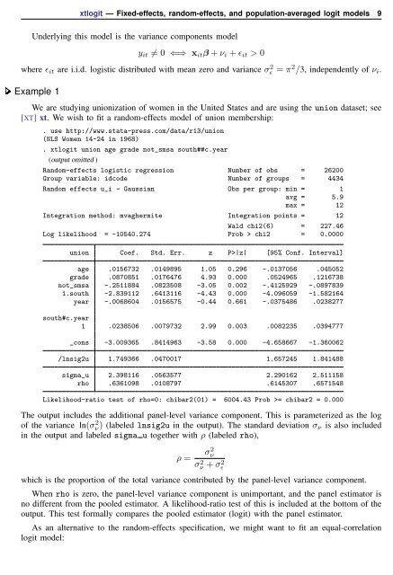
xtlogit — Fixed-effects, random-effects, and population-averaged logit models 9 Underlying this model is the variance components model y it ≠ 0 ⇐⇒ x it β + ν i + ɛ it > 0 where ɛ it are i.i.d. logistic distributed with mean zero and variance σ 2 ɛ = π 2 /3, independently of ν i . Example 1 We are studying unionization of women in the United States and are using the union dataset; see [XT] xt. We wish to fit a random-effects model of union membership: . use http://www.stata-press.com/data/r13/union (NLS Women 14-24 in 1968) . xtlogit union age grade not_smsa south##c.year (output omitted ) Random-effects logistic regression Number of obs = 26200 Group variable: idcode Number of groups = 4434 Random effects u_i ~ Gaussian Obs per group: min = 1 avg = 5.9 max = 12 Integration method: mvaghermite Integration points = 12 Wald chi2(6) = 227.46 Log likelihood = -10540.274 Prob > chi2 = 0.0000 union Coef. Std. Err. z P>|z| [95% Conf. Interval] age .0156732 .0149895 1.05 0.296 -.0137056 .045052 grade .0870851 .0176476 4.93 0.000 .0524965 .1216738 not_smsa -.2511884 .0823508 -3.05 0.002 -.4125929 -.0897839 1.south -2.839112 .6413116 -4.43 0.000 -4.096059 -1.582164 year -.0068604 .0156575 -0.44 0.661 -.0375486 .0238277 south#c.year 1 .0238506 .0079732 2.99 0.003 .0082235 .0394777 _cons -3.009365 .8414963 -3.58 0.000 -4.658667 -1.360062 /lnsig2u 1.749366 .0470017 1.657245 1.841488 sigma_u 2.398116 .0563577 2.290162 2.511158 rho .6361098 .0108797 .6145307 .6571548 Likelihood-ratio test of rho=0: chibar2(01) = 6004.43 Prob >= chibar2 = 0.000 The output includes the additional panel-level variance component. This is parameterized as the log of the variance ln(σ 2 ν) (labeled lnsig2u in the output). The standard deviation σ ν is also included in the output and labeled sigma u together with ρ (labeled rho), σ2 ν ρ = σν 2 + σɛ 2 which is the proportion of the total variance contributed by the panel-level variance component. When rho is zero, the panel-level variance component is unimportant, and the panel estimator is no different from the pooled estimator. A likelihood-ratio test of this is included at the bottom of the output. This test formally compares the pooled estimator (logit) with the panel estimator. As an alternative to the random-effects specification, we might want to fit an equal-correlation logit model:
- Page 1 and 2: Title stata.com xtlogit — Fixed-e
- Page 3 and 4: xtlogit — Fixed-effects, random-e
- Page 5 and 6: xtlogit — Fixed-effects, random-e
- Page 7: xtlogit — Fixed-effects, random-e
- Page 11 and 12: xtlogit — Fixed-effects, random-e
- Page 13 and 14: xtlogit — Fixed-effects, random-e
- Page 15 and 16: Methods and formulas xtlogit — Fi
- Page 17 and 18: xtlogit — Fixed-effects, random-e
<strong>xtlogit</strong> — Fixed-effects, random-effects, and population-averaged logit models 9<br />
Underlying this model is the variance components model<br />
y it ≠ 0 ⇐⇒ x it β + ν i + ɛ it > 0<br />
where ɛ it are i.i.d. logistic distributed with mean zero and variance σ 2 ɛ = π 2 /3, independently of ν i .<br />
Example 1<br />
We are studying unionization of women in the United States and are using the union dataset; see<br />
[XT] xt. We wish to fit a random-effects model of union membership:<br />
. use http://www.stata-press.com/data/r13/union<br />
(NLS Women 14-24 in 1968)<br />
. <strong>xtlogit</strong> union age grade not_smsa south##c.year<br />
(output omitted )<br />
Random-effects logistic regression Number of obs = 26200<br />
Group variable: idcode Number of groups = 4434<br />
Random effects u_i ~ Gaussian Obs per group: min = 1<br />
avg = 5.9<br />
max = 12<br />
Integration method: mvaghermite Integration points = 12<br />
Wald chi2(6) = 227.46<br />
Log likelihood = -10540.274 Prob > chi2 = 0.0000<br />
union Coef. Std. Err. z P>|z| [95% Conf. Interval]<br />
age .0156732 .0149895 1.05 0.296 -.0137056 .045052<br />
grade .0870851 .0176476 4.93 0.000 .0524965 .1216738<br />
not_smsa -.2511884 .0823508 -3.05 0.002 -.4125929 -.0897839<br />
1.south -2.839112 .6413116 -4.43 0.000 -4.096059 -1.582164<br />
year -.0068604 .0156575 -0.44 0.661 -.0375486 .0238277<br />
south#c.year<br />
1 .0238506 .0079732 2.99 0.003 .0082235 .0394777<br />
_cons -3.009365 .8414963 -3.58 0.000 -4.658667 -1.360062<br />
/lnsig2u 1.749366 .0470017 1.657245 1.841488<br />
sigma_u 2.398116 .0563577 2.290162 2.511158<br />
rho .6361098 .0108797 .6145307 .6571548<br />
Likelihood-ratio test of rho=0: chibar2(01) = 6004.43 Prob >= chibar2 = 0.000<br />
The output includes the additional panel-level variance component. This is parameterized as the log<br />
of the variance ln(σ 2 ν) (labeled lnsig2u in the output). The standard deviation σ ν is also included<br />
in the output and labeled sigma u together with ρ (labeled rho),<br />
σ2 ν<br />
ρ =<br />
σν 2 + σɛ<br />
2<br />
which is the proportion of the total variance contributed by the panel-level variance component.<br />
When rho is zero, the panel-level variance component is unimportant, and the panel estimator is<br />
no different from the pooled estimator. A likelihood-ratio test of this is included at the bottom of the<br />
output. This test formally compares the pooled estimator (logit) with the panel estimator.<br />
As an alternative to the random-effects specification, we might want to fit an equal-correlation<br />
logit model:


