meglm postestimation - Stata

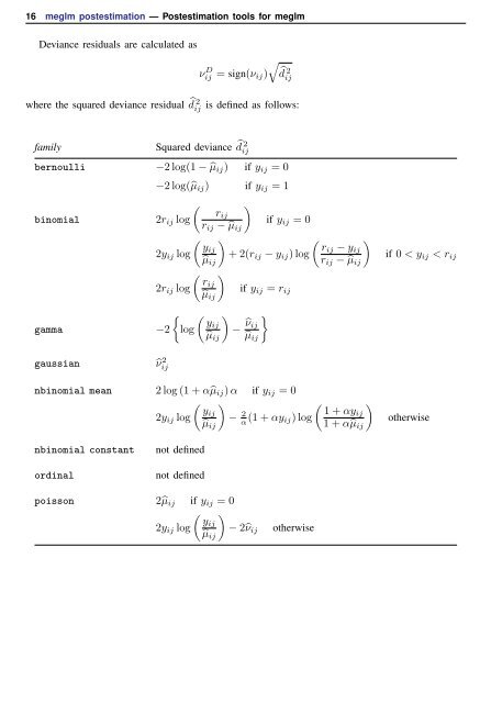
16 meglm postestimation — Postestimation tools for meglm
Deviance residuals are calculated as
ν D ij = sign(ν ij )√
̂d
2
ij
where the squared deviance residual ̂d 2 ij
is defined as follows:
family
Squared deviance ̂d 2 ij
bernoulli −2 log(1 − ̂µ ij ) if y ij = 0
binomial
gamma
−2 log(̂µ ij ) if y ij = 1
(
rij
2r ij log
(
yij
2y ij log
r ij − ̂µ ij
)
( )
rij
2r ij log
̂µ ij
if y ij = 0
̂µ ij
)
+ 2(r ij − y ij ) log
if y ij = r ij
{ ( )
yij
−2 log − ̂ν }
ij
̂µ ij ̂µ ij
( )
rij − y ij
r ij − ̂µ ij
if 0 < y ij < r ij
gaussian
̂ν 2 ij
nbinomial mean 2 log (1 + α̂µ ij ) α if y ij = 0
( )
( )
yij
1 +
2y ij log −
̂µ 2 ij
α (1 + αy αyij
ij) log
1 + α̂µ ij
otherwise
nbinomial constant
ordinal
not defined
not defined
poisson 2̂µ ij if y ij = 0
2y ij log
(
yij
̂µ ij
)
− 2̂ν ij
otherwise