SVY - Stata

Title 

stata.com 

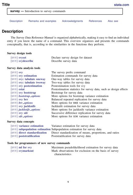
survey — Introduction to survey commands 

Description Remarks and examples Acknowledgments References Also see 

Description 

The Survey Data Reference Manual is organized alphabetically, making it easy to find an individual 

entry if you know the name of a command. This overview organizes and presents the commands 

conceptually, that is, according to the similarities in the functions they perform. 

Survey design tools 

[SVY] svyset 

[SVY] svydescribe 

Declare survey design for dataset 

Describe survey data 

Survey data analysis tools 

[SVY] svy 

[SVY] svy estimation 

[SVY] svy: tabulate oneway 

[SVY] svy: tabulate twoway 

[SVY] svy postestimation 

[SVY] estat 

[SVY] svy bootstrap 

[SVY] bootstrap options 

[SVY] svy brr 

[SVY] brr options 

[SVY] svy jackknife 

[SVY] jackknife options 

[SVY] svy sdr 

[SVY] sdr options 

Survey data concepts 

The survey prefix command 

Estimation commands for survey data 

One-way tables for survey data 

Two-way tables for survey data 

Postestimation tools for svy 

Postestimation statistics for survey data, such as design effects 

Bootstrap for survey data 

More options for bootstrap variance estimation 

Balanced repeated replication for survey data 

More options for BRR variance estimation 

Jackknife estimation for survey data 

More options for jackknife variance estimation 

Successive difference replication for survey data 

More options for SDR variance estimation 

[SVY] variance estimation Variance estimation for survey data 

[SVY] subpopulation estimation Subpopulation estimation for survey data 

[SVY] direct standardization Direct standardization of means, proportions, and ratios 

[SVY] poststratification Poststratification for survey data 

Tools for programmers of new survey commands 

[SVY] ml for svy 

[SVY] svymarkout 

Maximum pseudolikelihood estimation for survey data 

Mark observations for exclusion on the basis of survey 

characteristics 

1

2 survey — Introduction to survey commands 

Remarks and examples 

stata.com 

Remarks are presented under the following headings: 

Introduction 





Video example 

Introduction 

Stata’s facilities for survey data analysis are centered around the svy prefix command. After you 

identify the survey design characteristics with the svyset command, prefix the estimation commands 

in your data analysis with “svy:”. For example, where you would normally use the regress command 

to fit a linear regression model for nonsurvey data, use svy: regress to fit a linear regression model 

for your survey data. 

Why should you use the svy prefix command when you have survey data? To answer this question, 

we need to discuss some of the characteristics of survey design and survey data collection because 

these characteristics affect how we must perform our analysis if we want to get it right. 

Survey data are characterized by the following: 

• Sampling weights, also called probability weights—pweights in Stata’s terminology 

• Cluster sampling 

• Stratification 

These features arise from the design and details of the data collection procedure. Here’s a brief 

description of how these design features affect the analysis of the data: 

• Sampling weights. In sample surveys, observations are selected through a random process, 

but different observations may have different probabilities of selection. Weights are equal to 

(or proportional to) the inverse of the probability of being sampled. Various postsampling 

adjustments to the weights are sometimes made, as well. A weight of w j for the jth observation 

means, roughly speaking, that the jth observation represents w j elements in the population 

from which the sample was drawn. 

Omitting weights from the analysis results in estimates that may be biased, sometimes seriously 

so. Sampling weights also play a role in estimating standard errors. 

• Clustering. Individuals are not sampled independently in most survey designs. Collections of 

individuals (for example, counties, city blocks, or households) are typically sampled as a group, 

known as a cluster. 

There may also be further subsampling within the clusters. For example, counties may be 

sampled, then city blocks within counties, then households within city blocks, and then finally 

persons within households. The clusters at the first level of sampling are called primary sampling 

units (PSUs)—in this example, counties are the PSUs. In the absence of clustering, the PSUs 

are defined to be the individuals, or, equivalently, clusters, each of size one. 

Cluster sampling typically results in larger sample-to-sample variability than sampling individuals 

directly. This increased variability must be accounted for in standard error estimates, hypothesis 

testing, and other forms of inference.

survey — Introduction to survey commands 3 

• Stratification. In surveys, different groups of clusters are often sampled separately. These groups 

are called strata. For example, the 254 counties of a state might be divided into two strata, say, 

urban counties and rural counties. Then 10 counties might be sampled from the urban stratum, 

and 15 from the rural stratum. 

Sampling is done independently across strata; the stratum divisions are fixed in advance. Thus 

strata are statistically independent and can be analyzed as such. When the individual strata 

are more homogeneous than the population as a whole, the homogeneity can be exploited to 

produce smaller (and honestly so) estimates of standard errors. 

To put it succinctly: using sampling weights is important to get the point estimates right. We must 

consider the weighting, clustering, and stratification of the survey design to get the standard errors 

right. If our analysis ignores the clustering in our design, we would probably produce standard errors 

that are smaller than they should be. Stratification can be used to get smaller standard errors for a 

given overall sample size. 

For more detailed introductions to complex survey data analysis, see Cochran (1977); Heeringa, 

West, and Berglund (2010); Kish (1965); Levy and Lemeshow (2008); Scheaffer et al.; (2012); 

Skinner, Holt, and Smith (1989); Stuart (1984); Thompson (2012); and Williams (1978). 


Before using svy, first take a quick look at [SVY] svyset. Use the svyset command to specify 

the variables that identify the survey design characteristics and default method for estimating standard 

errors. Once set, svy will automatically use these design specifications until they are cleared or 

changed or a new dataset is loaded into memory. 

As the following two examples illustrate, svyset allows you to identify a wide range of complex 

sampling designs. First, we show a simple single-stage design and then a complex multistage design. 

Example 1: Survey data from a one-stage design 

A commonly used single-stage survey design uses clustered sampling across several strata, where 

the clusters are sampled without replacement. In a Stata dataset composed of survey data from this 

design, the survey design variables identify information about the strata, PSUs (clusters), sampling 

weights, and finite population correction. Here we use svyset to specify these variables, respectively 

named strata, su1, pw, and fpc1. 

. use http://www.stata-press.com/data/r13/stage5a 

. svyset su1 [pweight=pw], strata(strata) fpc(fpc1) 

pweight: pw 

VCE: linearized 

Single unit: missing 

Strata 1: strata 

SU 1: su1 

FPC 1: fpc1 

In addition to the variables we specified, svyset reports that the default method for estimating 

standard errors is Taylor linearization and that svy will report missing values for the standard errors 

when it encounters a stratum with one sampling unit (also called singleton strata).


Example 2: Multistage survey data 

We have (fictional) data on American high school seniors (12th graders), and the data were collected 

according to the following multistage design. In the first stage, counties were independently selected 

within each state. In the second stage, schools were selected within each chosen county. Within each 

chosen school, a questionnaire was filled out by every attending high school senior. We have entered 

all the information into a Stata dataset called multistage.dta. 

The survey design variables are as follows: 

• state contains the stratum identifiers. 

• county contains the first-stage sampling units. 

• ncounties contains the total number of counties within each state. 

• school contains the second-stage sampling units. 

• nschools contains the total number of schools within each county. 

• sampwgt contains the sampling weight for each sampled individual. 

Here we load the dataset into memory and use svyset with the above variables to declare that 

these data are survey data. 

. use http://www.stata-press.com/data/r13/multistage 

. svyset county [pw=sampwgt], strata(state) fpc(ncounties) || school, fpc(nschools) 

pweight: sampwgt 



Strata 1: state 

SU 1: county 

FPC 1: ncounties 

Strata 2: 

SU 2: school 

FPC 2: nschools 

. save highschool 

file highschool.dta saved 

We saved the svyset dataset to highschool.dta. We can now use this new dataset without having 

to worry about respecifying the design characteristics. 

. clear 

. describe 

Contains data 

obs: 0 

vars: 0 

size: 0 

Sorted by: 

. use highschool 

. svyset 





SU 1: county 


Strata 2: 

SU 2: school 

FPC 2: nschools


After the design characteristics have been svyset, you should also look at [SVY] svydescribe. Use 

svydescribe to browse each stage of your survey data; svydescribe reports useful information 

on sampling unit counts, missing data, and singleton strata. 

Example 3: Survey describe 

Here we use svydescribe to describe the first stage of our survey dataset of sampled high school 

seniors. We specified the weight variable to get svydescribe to report on where it contains missing 

values and how this affects the estimation sample. 

. svydescribe weight 

Survey: Describing stage 1 sampling units 





SU 1: county 


Strata 2: 

SU 2: school 

FPC 2: nschools 

#Obs with #Obs with #Obs per included Unit 

#Units #Units complete missing 

Stratum included omitted data data min mean max 

1 2 0 92 0 34 46.0 58 

2 2 0 112 0 51 56.0 61 

3 2 0 43 0 18 21.5 25 

4 2 0 37 0 14 18.5 23 

5 2 0 96 0 38 48.0 58 

(output omitted ) 

46 2 0 115 0 56 57.5 59 

47 2 0 67 0 28 33.5 39 

48 2 0 56 0 23 28.0 33 

49 2 0 78 0 39 39.0 39 

50 2 0 64 0 31 32.0 33 

50 100 0 4071 0 14 40.7 81 

4071 

From the output, we gather that there are 50 strata, each stratum contains two PSUs, the PSUs vary 

in size, and the total sample size is 4,071 students. We can also see that there are no missing data 

in the weight variable. 


Stata’s suite of survey data commands is governed by the svy prefix command; see [SVY] svy and 

[SVY] svy estimation. svy runs the supplied estimation command while accounting for the survey 

design characteristics in the point estimates and variance estimation method. The available variance 

estimation methods are balanced repeated replication (BRR), the bootstrap, the jackknife, successive 

difference replication, and first-order Taylor linearization. By default, svy computes standard errors 

by using the linearized variance estimator—so called because it is based on a first-order Taylor series 

linear approximation (Wolter 2007). In the nonsurvey context, we refer to this variance estimator as 

the robust variance estimator, otherwise known in Stata as the Huber/White/sandwich estimator; see 

[P] robust.


Example 4: Estimating a population mean 

Here we use the svy prefix with the mean command to estimate the average weight of high school 

seniors in our population. 

. svy: mean weight 

(running mean on estimation sample) 

Survey: Mean estimation 

Number of strata = 50 Number of obs = 4071 

Number of PSUs = 100 Population size = 8000000 

Design df = 50 

Linearized 

Mean Std. Err. [95% Conf. Interval] 

weight 160.2863 .7412512 158.7974 161.7751 

In its header, svy reports the number of strata and PSUs from the first stage, the sample size, an 

estimate of population size, and the design degrees of freedom. Just like the standard output from 

the mean command, the table of estimation results contains the estimated mean and its standard error 

as well as a confidence interval. 

Example 5: Survey regression 

Here we use the svy prefix with the regress command to model the association between weight 

and height in our population of high school seniors. 

. svy: regress weight height 

(running regress on estimation sample) 

Survey: Linear regression 




F( 1, 50) = 593.99 

Prob > F = 0.0000 

R-squared = 0.2787 

Linearized 

weight Coef. Std. Err. t P>|t| [95% Conf. Interval] 

height .7163115 .0293908 24.37 0.000 .6572784 .7753447 

_cons -149.6183 12.57265 -11.90 0.000 -174.8712 -124.3654 

In addition to the header elements we saw in the previous example using svy: mean, the command 

svy: regress also reports a model F test and estimated R 2 . Although many of Stata’s model-fitting 

commands report Z statistics for testing coefficients against zero, svy always reports t statistics and 

uses the design degrees of freedom to compute p-values.


The svy prefix can be used with many estimation commands in Stata. Here is the list of estimation 

commands that support the svy prefix. 

Descriptive statistics 

mean [R] mean — Estimate means 

proportion [R] proportion — Estimate proportions 

ratio [R] ratio — Estimate ratios 

total [R] total — Estimate totals 

Linear regression models 

cnsreg [R] cnsreg — Constrained linear regression 

etregress [TE] etregress — Linear regression with endogenous treatment effects 

glm [R] glm — Generalized linear models 

intreg [R] intreg — Interval regression 

nl 

[R] nl — Nonlinear least-squares estimation 

regress [R] regress — Linear regression 

tobit [R] tobit — Tobit regression 

truncreg [R] truncreg — Truncated regression 

Structural equation models 

sem [SEM] sem — Structural equation model estimation command 

Survival-data regression models 

stcox [ST] stcox — Cox proportional hazards model 

streg [ST] streg — Parametric survival models 

Binary-response regression models 

biprobit [R] biprobit — Bivariate probit regression 

cloglog [R] cloglog — Complementary log-log regression 

hetprobit [R] hetprobit — Heteroskedastic probit model 

logistic [R] logistic — Logistic regression, reporting odds ratios 

logit [R] logit — Logistic regression, reporting coefficients 

probit [R] probit — Probit regression 

scobit [R] scobit — Skewed logistic regression 

Discrete-response regression models 

clogit [R] clogit — Conditional (fixed-effects) logistic regression 

mlogit [R] mlogit — Multinomial (polytomous) logistic regression 

mprobit [R] mprobit — Multinomial probit regression 

ologit [R] ologit — Ordered logistic regression 

oprobit [R] oprobit — Ordered probit regression 

slogit [R] slogit — Stereotype logistic regression


Poisson regression models 

gnbreg Generalized negative binomial regression in [R] nbreg 

nbreg [R] nbreg — Negative binomial regression 

poisson [R] poisson — Poisson regression 

tnbreg [R] tnbreg — Truncated negative binomial regression 

tpoisson [R] tpoisson — Truncated Poisson regression 

zinb [R] zinb — Zero-inflated negative binomial regression 

zip 

[R] zip — Zero-inflated Poisson regression 

Instrumental-variables regression models 

ivprobit [R] ivprobit — Probit model with continuous endogenous regressors 

ivregress [R] ivregress — Single-equation instrumental-variables regression 

ivtobit [R] ivtobit — Tobit model with continuous endogenous regressors 

Regression models with selection 

heckman [R] heckman — Heckman selection model 

heckoprobit [R] heckoprobit — Ordered probit model with sample selection 

heckprobit [R] heckprobit — Probit model with sample selection 

Example 6: Cox’s proportional hazards model 

Suppose that we want to model the incidence of lung cancer by using three risk factors: smoking 

status, sex, and place of residence. Our dataset comes from a longitudinal health survey: the First 

National Health and Nutrition Examination Survey (NHANES I) (Miller 1973; Engel et al. 1978) and its 

1992 Epidemiologic Follow-up Study (NHEFS) (Cox et al. 1997); see the National Center for Health 

Statistics website at http://www.cdc.gov/nchs/. We will be using data from the samples identified by 

NHANES I examination locations 1–65 and 66–100; thus we will svyset the revised pseudo-PSU and 

strata variables associated with these locations. Similarly, our pweight variable was generated using 

the sampling weights for the nutrition and detailed samples for locations 1–65 and the weights for 

the detailed sample for locations 66–100. 

. use http://www.stata-press.com/data/r13/nhefs 

. svyset psu2 [pw=swgt2], strata(strata2) 

pweight: swgt2 



Strata 1: strata2 

SU 1: psu2 

FPC 1: 

The lung cancer information was taken from the 1992 NHEFS interview data. We use the participants’ 

ages for the time scale. Participants who never had lung cancer and were alive for the 1992 interview 

were considered censored. Participants who never had lung cancer and died before the 1992 interview 

were also considered censored at their age of death.


. stset age_lung_cancer [pw=swgt2], fail(lung_cancer) 

failure event: lung_cancer != 0 & lung_cancer < . 

obs. time interval: (0, age_lung_cancer] 

exit on or before: failure 

weight: [pweight=swgt2] 

14407 total observations 

5126 event time missing (age_lung_cancer>=.) PROBABLE ERROR 

9281 observations remaining, representing 

83 failures in single-record/single-failure data 

599691 total analysis time at risk and under observation 

at risk from t = 0 

earliest observed entry t = 0 

last observed exit t = 97 

Although stset warns us that it is a “probable error” to have 5,126 observations with missing event 

times, we can verify from the 1992 NHEFS documentation that there were indeed 9,281 participants 

with complete information. 

For our proportional hazards model, we pulled the risk factor information from the NHANES I and 

1992 NHEFS datasets. Smoking status was taken from the 1992 NHEFS interview data, but we filled 

in all but 132 missing values by using the general medical history supplement data in NHANES I. 

Smoking status is represented by separate indicator variables for former smokers and current smokers; 

the base comparison group is nonsmokers. Sex was determined using the 1992 NHEFS vitality data 

and is represented by an indicator variable for males. Place-of-residence information was taken from 

the medical history questionnaire in NHANES I and is represented by separate indicator variables for 

rural and heavily populated (more than 1 million people) urban residences; the base comparison group 

is urban residences with populations of fewer than 1 million people. 

. svy: stcox former_smoker smoker male urban1 rural 

(running stcox on estimation sample) 

Survey: Cox regression 




F( 5, 66) = 14.07 

Prob > F = 0.0000 

Linearized 

_t Haz. Ratio Std. Err. t P>|t| [95% Conf. Interval] 

former_smoker 2.788113 .6205102 4.61 0.000 1.788705 4.345923 

smoker 7.849483 2.593249 6.24 0.000 4.061457 15.17051 

male 1.187611 .3445315 0.59 0.555 .6658757 2.118142 

urban1 .8035074 .3285144 -0.54 0.594 .3555123 1.816039 

rural 1.581674 .5281859 1.37 0.174 .8125799 3.078702 

From the above results, we can see that both former and current smokers have a significantly 

higher risk for developing lung cancer than do nonsmokers.


svy: tabulate can be used to produce one-way and two-way tables with survey data and can 

produce survey-adjusted tests of independence for two-way contingency tables; see [SVY] svy: tabulate 

oneway and [SVY] svy: tabulate twoway. 

Example 7: Two-way tables for survey data 

With data from the Second National Health and Nutrition Examination Survey (NHANES II) 

(McDowell et al. 1981), we use svy: tabulate to produce a two-way table of cell proportions along 

with their standard errors and confidence intervals (the survey design characteristics have already 

been svyset). We also use the format() option to get svy: tabulate to report the cell values 

and marginals to four decimal places. 

. use http://www.stata-press.com/data/r13/nhanes2b 

. svy: tabulate race diabetes, row se ci format(%7.4f) 

(running tabulate on estimation sample) 




1=white, 

2=black, 

diabetes, 1=yes, 0=no 

3=other 0 1 Total 

Key: 

White 0.9680 0.0320 1.0000 

(0.0020) (0.0020) 

[0.9638,0.9718] [0.0282,0.0362] 

Black 0.9410 0.0590 1.0000 

(0.0061) (0.0061) 

[0.9271,0.9523] [0.0477,0.0729] 

Other 0.9797 0.0203 1.0000 

(0.0076) (0.0076) 

[0.9566,0.9906] [0.0094,0.0434] 

Total 0.9658 0.0342 1.0000 

(0.0018) (0.0018) 

[0.9619,0.9693] [0.0307,0.0381] 

row proportions 

(linearized standard errors of row proportions) 

[95% confidence intervals for row proportions] 

Pearson: 

Uncorrected chi2(2) = 21.3483 

Design-based F(1.52, 47.26) = 15.0056 P = 0.0000 

svy: tabulate has many options, such as the format() option, for controlling how the table 

looks. See [SVY] svy: tabulate twoway for a discussion of the different design-based and unadjusted 

tests of association.


All the standard postestimation commands (for example, estimates, lincom, margins, nlcom, 

test, testnl) are also available after svy. 

Example 8: Comparing means 

Going back to our high school survey data in example 2, we estimate the mean of weight (in 

pounds) for each subpopulation identified by the categories of the sex variable (male and female). 

. use http://www.stata-press.com/data/r13/highschool 

. svy: mean weight, over(sex) 






male: sex = male 

female: sex = female 

Linearized 

Over Mean Std. Err. [95% Conf. Interval] 

weight 

male 175.4809 1.116802 173.2377 177.7241 

female 146.204 .9004157 144.3955 148.0125 

Here we use the test command to test the hypothesis that the average male is 30 pounds heavier 

than the average female; from the results, we cannot reject this hypothesis at the 5% level. 

. test [weight]male - [weight]female = 30 

Adjusted Wald test 

( 1) [weight]male - [weight]female = 30 

F( 1, 50) = 0.23 

Prob > F = 0.6353 

estat has specific subroutines for use after svy; see [SVY] estat. 

• estat svyset reports the survey design settings used to produce the current estimation results. 

• estat effects and estat lceffects report a table of design and misspecification effects 

for point estimates and linear combinations of point estimates, respectively. 

• estat size reports a table of sample and subpopulation sizes after svy: mean, svy: proportion, 

svy: ratio, and svy: total. 

• estat sd reports subpopulation standard deviations on the basis of the estimation results from 

mean and svy: mean. 

• estat strata reports the number of singleton and certainty strata within each sampling stage. 

• estat cv reports the coefficient of variation for each coefficient in the current estimation results. 

• estat gof reports a goodness-of-fit test for binary response models using survey data.


Example 9: Design effects 

Here we use estat effects to report the design effects DEFF and DEFT for the mean estimates 

from the previous example. 

. estat effects 

male: sex = male 

female: sex = female 

Linearized 

Over Mean Std. Err. DEFF DEFT 

weight 

male 175.4809 1.116802 2.61016 1.61519 

female 146.204 .9004157 1.7328 1.31603 

Note: weights must represent population totals for deff to 

be correct when using an FPC; however, deft is 

invariant to the scale of weights. 

Now we use estat lceffects to report the design effects DEFF and DEFT for the difference of 

the mean estimates from the previous example. 

. estat lceffects [weight]male - [weight]female 

( 1) [weight]male - [weight]female = 0 

Mean Coef. Std. Err. DEFF DEFT 

(1) 29.27691 1.515201 2.42759 1.55768 

Note: weights must represent population totals for deff to 

be correct when using an FPC; however, deft is 

invariant to the scale of weights. 

The svy brr prefix command produces point and variance estimates by using the BRR method; 

see [SVY] svy brr. BRR was first introduced by McCarthy (1966, 1969a, and 1969b) as a method of 

variance estimation for designs with two PSUs in every stratum. The BRR variance estimator tends to 

give more reasonable variance estimates for this design than the linearized variance estimator, which 

can result in large values and undesirably wide confidence intervals. 

The svy jackknife prefix command produces point and variance estimates by using the jackknife 

replication method; see [SVY] svy jackknife. The jackknife is a data-driven variance estimation 

method that can be used with model-fitting procedures for which the linearized variance estimator is 

not implemented, even though a linearized variance estimator is theoretically possible to derive (Shao 

and Tu 1995). 

To protect the privacy of survey participants, public survey datasets may contain replicate-weight 

variables instead of variables that identify the PSUs and strata. These replicate-weight variables can be 

used with the appropriate replication method for variance estimation instead of the linearized variance 

estimator; see [SVY] svyset. 

The svy brr and svy jackknife prefix commands can be used with those commands that may 

not be fully supported by svy but are compatible with the BRR and the jackknife replication methods. 

They can also be used to produce point estimates for expressions of estimation results from a prefixed 

command. 

The svy bootstrap and svy sdr prefix commands work only with replicate weights. Both assume 

that you have obtained these weight variables externally.


The svy bootstrap prefix command produces variance estimates that have been adjusted for 

bootstrap sampling. Bootstrap sampling of complex survey has become more popular in recent years 

and is the variance-estimation method used in the National Population Health Survey conducted by 

Statistics Canada; see [SVY] svy bootstrap and [SVY] variance estimation for more details. 

The svy sdr prefix command produces variance estimates that implement successive difference 

replication (SDR), first introduced by Fay and Train (1995) as a method for annual demographic 

supplements to the Current Population Survey. This method is typically applied to systematic samples 

where the observed sampling units follow a natural order; see [SVY] svy sdr and [SVY] variance 

estimation for more details. 

Example 10: BRR and replicate-weight variables 

The survey design for the NHANES II data (McDowell et al. 1981) is specifically suited to BRR: 

there are two PSUs in every stratum. 

. use http://www.stata-press.com/data/r13/nhanes2 

. svydescribe 

Survey: Describing stage 1 sampling units 

pweight: finalwgt 



Strata 1: strata 

SU 1: psu 

FPC 1: 

#Obs per Unit 

Stratum #Units #Obs min mean max 

1 2 380 165 190.0 215 

2 2 185 67 92.5 118 

3 2 348 149 174.0 199 

4 2 460 229 230.0 231 

5 2 252 105 126.0 147 

(output omitted ) 

29 2 503 215 251.5 288 

30 2 365 166 182.5 199 

31 2 308 143 154.0 165 

32 2 450 211 225.0 239 

31 62 10351 67 167.0 288 

Here is a privacy-conscious dataset equivalent to the one above; all the variables and values 

remain, except that strata and psu are replaced with BRR replicate-weight variables. The BRR 

replicate-weight variables are already svyset, and the default method for variance estimation is 

vce(brr).


. use http://www.stata-press.com/data/r13/nhanes2brr 

. svyset 

pweight: finalwgt 

VCE: brr 

MSE: off 

brrweight: brr_1 brr_2 brr_3 brr_4 brr_5 brr_6 brr_7 brr_8 brr_9 brr_10 

brr_11 brr_12 brr_13 brr_14 brr_15 brr_16 brr_17 brr_18 brr_19 

brr_20 brr_21 brr_22 brr_23 brr_24 brr_25 brr_26 brr_27 brr_28 

brr_29 brr_30 brr_31 brr_32 


Strata 1: 

SU 1: 

FPC 1: 

Suppose that we were interested in the population ratio of weight to height. Here we use total 

to estimate the population totals of weight and height and the svy brr prefix to estimate their ratio 

and variance; we use total instead of ratio (which is otherwise preferable here) to show how to 

specify an expression when using svy: brr. 

. svy brr WtoH = (_b[weight]/_b[height]): total weight height 

(running total on estimation sample) 

BRR replications (32) 

1 2 3 4 5 

................................ 

BRR results Number of obs = 10351 

Population size = 117157513 

Replications = 32 


command: 

WtoH: 

total weight height 

_b[weight]/_b[height] 

BRR 

Coef. Std. Err. t P>|t| [95% Conf. Interval] 

WtoH .4268116 .0008904 479.36 0.000 .4249957 .4286276 


The variance estimation methods that Stata uses are discussed in [SVY] variance estimation. 

Subpopulation estimation involves computing point and variance estimates for part of the population. 

This method is not the same as restricting the estimation sample to the collection of observations 

within the subpopulation because variance estimation for survey data measures sample-to-sample 

variability, assuming that the same survey design is used to collect the data. Use the subpop() option 

of the svy prefix to perform subpopulation estimation, and use if and in only when you need to 

make restrictions on the estimation sample; see [SVY] subpopulation estimation. 

Example 11: Subpopulation estimation 

Here we will use our svyset high school data to model the association between weight and 

height in the subpopulation of male high school seniors. First, we describe the sex variable to 

determine how to identify the males in the dataset. We then use label list to verify that the variable 

label agrees with the value labels.



. describe sex 

storage display value 

variable name type format label variable label 

sex byte %9.0g sex 1=male, 2=female 

. label list sex 

sex: 

1 male 

2 female 

Here we generate a variable named male so that we can easily identify the male high school 

seniors. We specified if !missing(sex); doing so will cause the generated male variable to contain 

a missing value at each observation where the sex variable does. This is done on purpose (although it 

is not necessary if sex is free of missing values) because missing values should not be misinterpreted 

to imply female. 

. generate male = sex == 1 if !missing(sex) 

Now we specify subpop(male) as an option to the svy prefix in our model fit. 

. svy, subpop(male): regress weight height 

(running regress on estimation sample) 

Survey: Linear regression 



Subpop. no. of obs = 1938 

Subpop. size = 3848021.4 


F( 1, 50) = 225.38 

Prob > F = 0.0000 

R-squared = 0.2347 

Linearized 


height .7632911 .0508432 15.01 0.000 .6611696 .8654127 

_cons -168.6532 22.5708 -7.47 0.000 -213.988 -123.3184 

Although the table of estimation results contains the same columns as earlier, svy reports some 

extra subpopulation information in the header. Here the extra header information tells us that 1,938 

of the 4,071 sampled high school seniors are male, and the estimated number of male high school 

seniors in the population is 3,848,021 (rounded down). 

Direct standardization is an estimation method that allows comparing rates that come from different 

frequency distributions; see [SVY] direct standardization. In direct standardization, estimated rates 

(means, proportions, and ratios) are adjusted according to the frequency distribution of a standard 

population. The standard population is partitioned into categories, called standard strata. The stratum 

frequencies for the standard population are called standard weights. In the standardizing frequency 

distribution, the standard strata are most commonly identified by demographic information such as 

age, sex, and ethnicity. The standardized rate estimate is the weighted sum of unadjusted rates, where 

the weights are the relative frequencies taken from the standardizing frequency distribution. Direct 

standardization is available with svy: mean, svy: proportion, and svy: ratio.


Example 12: Standardized rates 

Table 3.12-6 of Korn and Graubard (1999, 156) contains enumerated data for two districts of 

London for the years 1840–1841. The age variable identifies the age groups in 5-year increments, 

bgliving contains the number of people living in the Bethnal Green district at the beginning of 

1840, bgdeaths contains the number of people who died in Bethnal Green that year, hsliving 

contains the number of people living in St. George’s Hanover Square at the beginning of 1840, and 

hsdeaths contains the number of people who died in Hanover Square that year. 

. use http://www.stata-press.com/data/r13/stdize, clear 

. list, noobs sep(0) sum 

age bgliving bgdeaths hsliving hsdeaths 

0-5 10739 850 5738 463 

5-10 9180 76 4591 55 

10-15 8006 38 4148 28 

15-20 7096 37 6168 36 

20-25 6579 38 9440 68 

25-30 5829 51 8675 78 

30-35 5749 51 7513 64 

35-40 4490 56 5091 78 

40-45 4385 47 4930 85 

45-50 2955 66 2883 66 

50-55 2995 74 2711 77 

55-60 1644 67 1275 55 

60-65 1835 64 1469 61 

65-70 1042 64 649 55 

70-75 879 68 619 58 

75-80 366 47 233 51 

80-85 173 39 136 20 

85-90 71 22 48 15 

90-95 21 6 10 4 

95-100 4 2 2 1 

unknown 50 1 124 0 

Sum 74088 1764 66453 1418 

We can use svy: ratio to compute the death rates for each district in 1840. Because this 

dataset is identified as census data, we will create an FPC variable that will contain a sampling 

rate of 100%. This method will result in zero standard errors, which are interpreted to mean no 

variability—appropriate because our point estimates came from the entire population.


. gen fpc = 1 

. svyset, fpc(fpc) 

pweight: 



Strata 1: 

SU 1: 

FPC 1: fpc 

. svy: ratio (Bethnal: bgdeaths/bgliving) (Hanover: hsdeaths/hsliving) 

(running ratio on estimation sample) 

Survey: Ratio estimation 




Bethnal: bgdeaths/bgliving 

Hanover: hsdeaths/hsliving 

Linearized 

Ratio Std. Err. [95% Conf. Interval] 

Bethnal .0238095 0 . . 

Hanover .0213384 0 . . 

Note: zero standard errors because of 100% sampling rate 

detected for FPC in the first stage. 

The death rates are 2.38% for Bethnal Green and 2.13% for St. George’s Hanover Square. These 

observed death rates are not really comparable because they come from two different age distributions. 

We can standardize based on the age distribution from Bethnal Green. Here age identifies our standard 

strata and bgliving contains the associated population sizes. 

. svy: ratio (Bethnal: bgdeaths/bgliving) (Hanover: hsdeaths/hsliving), 

> stdize(age) stdweight(bgliving) 

(running ratio on estimation sample) 

Survey: Ratio estimation 



N. of std strata = 21 Design df = 20 

Bethnal: bgdeaths/bgliving 

Hanover: hsdeaths/hsliving 

Linearized 

Ratio Std. Err. [95% Conf. Interval] 

Bethnal .0238095 0 . . 

Hanover .0266409 0 . . 

Note: zero standard errors because of 100% sampling rate 

detected for FPC in the first stage. 

The standardized death rate for St. George’s Hanover Square, 2.66%, is larger than the death rate 

for Bethnal Green. 

Poststratification is a method for adjusting the sampling weights, usually to account for underrepresented 

groups in the population; see [SVY] poststratification. This method usually results in 

decreasing bias because of nonresponse and underrepresented groups in the population. It also tends to


result in smaller variance estimates. Poststratification is available for all survey estimation commands 

and is specified using svyset; see [SVY] svyset. 

Example 13: Poststratified mean 

Levy and Lemeshow (2008, sec. 6.6) give an example of poststratification by using simple survey 

data from a veterinarian’s client list. The data in poststrata.dta were collected using simple 

random sampling (SRS) without replacement. The totexp variable contains the total expenses to the 

client, type identifies the cats and dogs, postwgt contains the poststratum sizes (450 for cats and 

850 for dogs), and fpc contains the total number of clients (850 + 450 = 1300). 

. use http://www.stata-press.com/data/r13/poststrata, clear 

. svyset, poststrata(type) postweight(postwgt) fpc(fpc) 

pweight: 


Poststrata: type 

Postweight: postwgt 


Strata 1: 

SU 1: 

FPC 1: fpc 

. svy: mean totexp 





N. of poststrata = 2 Design df = 49 

Linearized 


totexp 40.11513 1.163498 37.77699 42.45327 

The mean total expenses is $40.12 with a standard error of $1.16. In the following, we omit the 

poststratification information from svyset, resulting in mean total expenses of $39.73 with standard 

error $2.22. The difference between the mean estimates is explained by the facts that expenses tend 

to be larger for dogs than for cats and that the dogs were slightly underrepresented in the sample 

(850/1,300 ≈ 0.65 for the population; 32/50 = 0.64 for the sample). This reasoning also explains why 

the variance estimate from the poststratified mean is smaller than the one that was not poststratified.


. svyset, fpc(fpc) 

pweight: 



Strata 1: 

SU 1: 

FPC 1: fpc 

. svy: mean totexp 






Linearized 


totexp 39.7254 2.221747 35.26063 44.19017 


The ml command can be used to fit a model by the method of maximum likelihood. When the 

svy option is specified, ml performs maximum pseudolikelihood, applying sampling weights and 

design-based linearization automatically; see [R] ml and Gould, Pitblado, and Poi (2010). 

Example 14 

The ml command requires a program that computes likelihood values to perform maximum 

likelihood. Here is a likelihood evaluator used in Gould, Pitblado, and Poi (2010) to fit linear 

regression models using the likelihood from the normal distribution. 

program mynormal_lf 

version 13 

args lnf mu lnsigma 

quietly replace ‘lnf’ = ln(normalden($ML_y1,‘mu’,exp(‘lnsigma’))) 

end 

Back in example 5, we fit a linear regression model using the high school survey data. Here we 

use ml and mynormal lf to fit the same survey regression model.



. ml model lf mynormal_lf (mu: weight = height) /lnsigma, svy 

. ml max 

initial: log pseudolikelihood = - (could not be evaluated) 

feasible: log pseudolikelihood = -7.301e+08 

rescale: log pseudolikelihood = -51944380 

rescale eq: log pseudolikelihood = -47565331 

Iteration 0: log pseudolikelihood = -47565331 

Iteration 1: log pseudolikelihood = -41221759 (not concave) 







Iteration 8: log pseudolikelihood = -38467683 (backed up) 







F( 1, 50) = 593.99 

Prob > F = 0.0000 

Linearized 


mu 

height .7163115 .0293908 24.37 0.000 .6572784 .7753447 

_cons -149.6183 12.57265 -11.90 0.000 -174.8712 -124.3654 

lnsigma 

_cons 3.372154 .0180777 186.54 0.000 3.335844 3.408464 

svymarkout is a programmer’s command that resets the values in a variable that identifies the 

estimation sample, dropping observations for which any of the survey characteristic variables contain 

missing values. This tool is most helpful for developing estimation commands that use ml to fit 

models using maximum pseudolikelihood directly, instead of relying on the svy prefix. 

Video example 

Basic introduction to the analysis of complex survey data in Stata 

Acknowledgments 

Many of the svy commands were developed in collaboration with John L. Eltinge of the Bureau 

of Labor Statistics. We thank him for his invaluable assistance. 

We thank Wayne Johnson of the National Center for Health Statistics for providing the NHANES II 

dataset.


We thank Nicholas Winter of the Politics Department at the University of Virginia for his diligent 

efforts to keep Stata up to date with mainstream variance estimation methods for survey data, as well 

as for providing versions of svy brr and svy jackknife. 

✄ 

✂ 

William Gemmell Cochran (1909–1980) was born in Rutherglen, Scotland, and educated at the 

Universities of Glasgow and Cambridge. He accepted a post at Rothamsted before finishing his 

doctorate. Cochran emigrated to the United States in 1939 and worked at Iowa State, North 

Carolina State, Johns Hopkins, and Harvard. He made many major contributions across several 

fields of statistics, including experimental design, the analysis of counted data, sample surveys, 

and observational studies, and was author or coauthor (with Gertrude M. Cox and George W. 

Snedecor) of various widely used texts. 

Leslie Kish (1910–2000) was born in Poprad, Hungary, and entered the United States with his 

family in 1926. He worked as a lab assistant at the Rockefeller Institute for Medical Research and 

studied at the College of the City of New York, fighting in the Spanish Civil War before receiving 

his first degree in mathematics. Kish worked for the Bureau of the Census, the Department of 

Agriculture, the Army Air Corps, and the University of Michigan. He carried out pioneering 

work in the theory and practice of survey sampling, including design effects, BRR, response 

errors, rolling samples and censuses, controlled selection, multipurpose designs, and small-area 

estimation. 

 

✁ 

References 

Cochran, W. G. 1977. Sampling Techniques. 3rd ed. New York: Wiley. 

Cox, C. S., M. E. Mussolino, S. T. Rothwell, M. A. Lane, C. D. Golden, J. H. Madans, and J. J. Feldman. 1997. 

Plan and operation of the NHANES I Epidemiologic Followup Study, 1992. In Vital and Health Statistics, series 1, 

no. 35. Hyattsville, MD: National Center for Health Statistics. 

Engel, A., R. S. Murphy, K. Maurer, and E. Collins. 1978. Plan and operation of the HANES I augmentation survey 

of adults 25–74 years: United States 1974–75. In Vital and Health Statistics, series 1, no. 14. Hyattsville, MD: 

National Center for Health Statistics. 

Fay, R. E., and G. F. Train. 1995. Aspects of survey and model-based postcensal estimation of income and poverty 

characteristics for states and counties. In Proceedings of the Government Statistics Section, 154–159. American 

Statistical Association. 

Gould, W. W., J. S. Pitblado, and B. P. Poi. 2010. Maximum Likelihood Estimation with Stata. 4th ed. College 

Station, TX: Stata Press. 

Heeringa, S. G., B. T. West, and P. A. Berglund. 2010. Applied Survey Data Analysis. Boca Raton, FL: Chapman 

& Hall/CRC. 

Kish, L. 1965. Survey Sampling. New York: Wiley. 

Korn, E. L., and B. I. Graubard. 1999. Analysis of Health Surveys. New York: Wiley. 

Kreuter, F., and R. Valliant. 2007. A survey on survey statistics: What is done and can be done in Stata. Stata Journal 

7: 1–21. 

Levy, P. S., and S. A. Lemeshow. 2008. Sampling of Populations: Methods and Applications. 4th ed. Hoboken, NJ: 

Wiley. 

McCarthy, P. J. 1966. Replication: An approach to the analysis of data from complex surveys. In Vital and Health 

Statistics, series 2. Hyattsville, MD: National Center for Health Statistics. 

. 1969a. Pseudoreplication: Further evaluation and application of the balanced half-sample technique. In Vital 

and Health Statistics, series 2. Hyattsville, MD: National Center for Health Statistics. 

. 1969b. Pseudo-replication: Half-samples. Revue de l’Institut International de Statistique 37: 239–264.


McDowell, A., A. Engel, J. T. Massey, and K. Maurer. 1981. Plan and operation of the Second National Health and 

Nutrition Examination Survey, 1976–1980. Vital and Health Statistics 1(15): 1–144. 

Miller, H. W. 1973. Plan and operation of the Health and Nutrition Examination Survey: United States 1971–1973. 

Hyattsville, MD: National Center for Health Statistics. 

Scheaffer, R. L., W. Mendenhall, III, R. L. Ott, and K. G. Gerow. 2012. Elementary Survey Sampling. 7th ed. 

Boston: Brooks/Cole. 

Shao, J., and D. Tu. 1995. The Jackknife and Bootstrap. New York: Springer. 

Skinner, C. J., D. Holt, and T. M. F. Smith, ed. 1989. Analysis of Complex Surveys. New York: Wiley. 

Stuart, A. 1984. The Ideas of Sampling. 3rd ed. New York: Griffin. 

Thompson, S. K. 2012. Sampling. 3rd ed. Hoboken, NJ: Wiley. 

Williams, B. 1978. A Sampler on Sampling. New York: Wiley. 

Wolter, K. M. 2007. Introduction to Variance Estimation. 2nd ed. New York: Springer. 

Also see 

[SVY] svyset — Declare survey design for dataset 

[SVY] svy — The survey prefix command 

[SVY] svy estimation — Estimation commands for survey data 

[P] robust — Robust variance estimates

SVY - Stata

Create successful ePaper yourself

Delete template?

Save as template?