arch postestimation - Stata

Title
stata.com
arch postestimation — Postestimation tools for arch
Description Syntax for predict Menu for predict Options for predict
Remarks and examples Also see
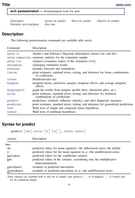
Description
The following postestimation commands are available after arch:
Command Description
estat ic Akaike’s and Schwarz’s Bayesian information criteria (AIC and BIC)
estat summarize summary statistics for the estimation sample
estat vce variance–covariance matrix of the estimators (VCE)
estimates cataloging estimation results
forecast dynamic forecasts and simulations
lincom
point estimates, standard errors, testing, and inference for linear combinations
of coefficients
lrtest
likelihood-ratio test
margins marginal means, predictive margins, marginal effects, and average marginal
effects
marginsplot graph the results from margins (profile plots, interaction plots, etc.)
nlcom
point estimates, standard errors, testing, and inference for nonlinear
combinations of coefficients
predict predictions, residuals, influence statistics, and other diagnostic measures
predictnl point estimates, standard errors, testing, and inference for generalized predictions
test
Wald tests of simple and composite linear hypotheses
testnl
Wald tests of nonlinear hypotheses
Syntax for predict
predict [ type ] newvar [ if ] [ in ] [ , statistic options ]
statistic
Main
xb
y
variance
het
residuals
yresiduals
Description
predicted values for mean equation—the differenced series; the default
predicted values for the mean equation in y—the undifferenced series
predicted values for the conditional variance
predicted values of the variance, considering only the multiplicative
heteroskedasticity
residuals or predicted innovations
residuals or predicted innovations in y—the undifferenced series
These statistics are available both in and out of sample; type predict . . . if e(sample) . . . if wanted only
for the estimation sample.
1

2 arch postestimation — Postestimation tools for arch
options
Options
dynamic(time constant)
at(varname ɛ | # ɛ varname σ 2 | # σ 2)
t0(time constant)
structural
Description
how to handle the lags of y t
make static predictions
set starting point for the recursions to time constant
calculate considering the structural component only
time constant is a # or a time literal, such as td(1jan1995) or tq(1995q1), etc.; see
Conveniently typing SIF values in [D] datetime.
Menu for predict
Statistics > Postestimation > Predictions, residuals, etc.
Options for predict
Six statistics can be computed by using predict after arch: the predictions of the mean equation
(option xb, the default), the undifferenced predictions of the mean equation (option y), the predictions
of the conditional variance (option variance), the predictions of the multiplicative heteroskedasticity
component of variance (option het), the predictions of residuals or innovations (option residuals),
and the predictions of residuals or innovations in terms of y (option yresiduals). Given the dynamic
nature of ARCH models and because the dependent variable might be differenced, there are other
ways of computing each statistic. We can use all the data on the dependent variable available right
up to the time of each prediction (the default, which is often called a one-step prediction), or we
can use the data up to a particular time, after which the predicted value of the dependent variable
is used recursively to make later predictions (option dynamic()). Either way, we can consider or
ignore the ARMA disturbance component, which is considered by default and is ignored if you specify
the structural option. We might also be interested in predictions at certain fixed points where we
specify the prior values of ɛ t and σt
2 (option at()).
✄
✄
Main
xb, the default, calculates the predictions from the mean equation. If D.depvar is the dependent
variable, these predictions are of D.depvar and not of depvar itself.
y specifies that predictions of depvar are to be made even if the model was specified for, say,
D.depvar.
variance calculates predictions of the conditional variance ̂σ 2 t .
het calculates predictions of the multiplicative heteroskedasticity component of variance.
residuals calculates the residuals. If no other options are specified, these are the predicted innovations
ɛ t ; that is, they include any ARMA component. If the structural option is specified, these are
the residuals from the mean equation, ignoring any ARMA terms; see structural below. The
residuals are always from the estimated equation, which may have a differenced dependent variable;
if depvar is differenced, they are not the residuals of the undifferenced depvar.
yresiduals calculates the residuals for depvar, even if the model was specified for, say, D.depvar. As
with residuals, the yresiduals are computed from the model, including any ARMA component.
If the structural option is specified, any ARMA component is ignored and yresiduals are the
residuals from the structural equation; see structural below.

✄
✄
Options
arch postestimation — Postestimation tools for arch 3
dynamic(time constant) specifies how lags of y t in the model are to be handled. If dynamic()
is not specified, actual values are used everywhere lagged values of y t appear in the model to
produce one-step-ahead forecasts.
dynamic(time constant) produces dynamic (also known as recursive) forecasts. time constant
specifies when the forecast is to switch from one step ahead to dynamic. In dynamic forecasts,
references to y t evaluate to the prediction of y t for all periods at or after time constant; they
evaluate to the actual value of y t for all prior periods.
dynamic(10), for example, would calculate predictions where any reference to y t with t < 10
evaluates to the actual value of y t and any reference to y t with t ≥ 10 evaluates to the prediction
of y t . This means that one-step-ahead predictions would be calculated for t < 10 and dynamic
predictions would be calculated thereafter. Depending on the lag structure of the model, the dynamic
predictions might still refer to some actual values of y t .
You may also specify dynamic(.) to have predict automatically switch from one-step-ahead to
dynamic predictions at p + q, where p is the maximum AR lag and q is the maximum MA lag.
at(varname ɛ | # ɛ varname σ 2 | # σ 2) makes static predictions. at() and dynamic() may not be
specified together.
Specifying at() allows static evaluation of results for a given set of disturbances. This is useful,
for instance, in generating the news response function. at() specifies two sets of values to be
used for ɛ t and σt 2 , the dynamic components in the model. These specified values are treated as
given. Also, any lagged values of depvar in the model are obtained from the real values of the
dependent variable. All computations are based on actual data and the given values.
at() requires that you specify two arguments, which can be either a variable name or a number.
The first argument supplies the values to be used for ɛ t ; the second supplies the values to be used
for σt 2. If σ2 t plays no role in your model, the second argument may be specified as ‘.’ to indicate
missing.
t0(time constant) specifies the starting point for the recursions to compute the predicted statistics;
disturbances are assumed to be 0 for t < t0(). The default is to set t0() to the minimum t
observed in the estimation sample, meaning that observations before that are assumed to have
disturbances of 0.
t0() is irrelevant if structural is specified because then all observations are assumed to have
disturbances of 0.
t0(5), for example, would begin recursions at t = 5. If your data were quarterly, you might
instead type t0(tq(1961q2)) to obtain the same result.
Any ARMA component in the mean equation or GARCH term in the conditional-variance equation
makes arch recursive and dependent on the starting point of the predictions. This includes
one-step-ahead predictions.
structural makes the calculation considering the structural component only, ignoring any ARMA
terms, and producing the steady-state equilibrium predictions.

4 arch postestimation — Postestimation tools for arch
Remarks and examples
stata.com
Example 1
Continuing with our EGARCH model example (example 3) in [TS] arch, we can see that predict,
at() calculates σ 2 t given a set of specified innovations (ɛ t, ɛ t−1 , . . .) and prior conditional variances
(σ 2 t−1, σ 2 t−2, . . .). The syntax is
. predict newvar, variance at(epsilon sigma2)
epsilon and sigma2 are either variables or numbers. Using sigma2 is a little tricky because you specify
values of σt 2 , which predict is supposed to predict. predict does not simply copy variable sigma2
into newvar but uses the lagged values contained in sigma2 to produce the predicted value of σt 2. It
does this for all t, and those results are saved in newvar. (If you are interested in dynamic predictions
of σt 2 , see Options for predict.)
We will generate predictions for σt 2, assuming that the lagged values of σ2 t are 1, and we will
vary ɛ t from −4 to 4. First, we will create variable et containing ɛ t , and then we will create and
graph the predictions:
. generate et = (_n-64)/15
. predict sigma2, variance at(et 1)
. line sigma2 et in 2/l, m(i) c(l) title(News response function)
News response function
Conditional variance, one−step
0 .5 1 1.5 2 2.5
−4 −2 0 2 4
et
The positive asymmetry does indeed dominate the shape of the news response function. In fact, the
response is a monotonically increasing function of news. The form of the response function shows
that, for our simple model, only positive, unanticipated price increases have the destabilizing effect
that we observe as larger conditional variances.

arch postestimation — Postestimation tools for arch 5
Example 2
Continuing with our ARCH model with constraints example (example 6) in [TS] arch, using lincom
we can recover the α parameter from the original specification.
. lincom [ARCH]l1.arch/.4
( 1) 2.5*[ARCH]L.arch = 0
D.ln_wpi Coef. Std. Err. z P>|z| [95% Conf. Interval]
(1) .5450344 .1844468 2.95 0.003 .1835253 .9065436
Any arch parameter could be used to produce an identical estimate.
Also see
[TS] arch — Autoregressive conditional heteroskedasticity (ARCH) family of estimators
[U] 20 Estimation and postestimation commands