

Tobit - Stata
Tobit - Stata
Tobit - Stata

You also want an ePaper? Increase the reach of your titles
YUMPU automatically turns print PDFs into web optimized ePapers that Google loves.
Title<br />
stata.com<br />
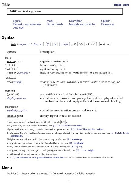
tobit — <strong>Tobit</strong> regression<br />
Syntax Menu Description Options<br />
Remarks and examples Stored results Methods and formulas References<br />
Also see<br />
Syntax<br />
tobit depvar [ indepvars ] [ if ] [ in ] [ weight ] , ll [ (#) ] ul [ (#) ] [ options ]<br />
options<br />
Description<br />
Model<br />
noconstant<br />
suppress constant term<br />
∗ ll [ (#) ]<br />
left-censoring limit<br />
∗ ul [ (#) ]<br />
right-censoring limit<br />
offset(varname) include varname in model with coefficient constrained to 1<br />
SE/Robust<br />
vce(vcetype)<br />
Reporting<br />
level(#)<br />
display options<br />
vcetype may be oim, robust, cluster clustvar, bootstrap, or<br />
jackknife<br />
set confidence level; default is level(95)<br />
control column formats, row spacing, line width, display of omitted<br />
variables and base and empty cells, and factor-variable labeling<br />
Maximization<br />
maximize options<br />
control the maximization process; seldom used<br />
coeflegend<br />
display legend instead of statistics<br />
] [ ]<br />
∗ You must specify at least one of ll<br />
[(#) or ul (#) .<br />
indepvars may contain factor variables; see [U] 11.4.3 Factor variables.<br />
depvar and indepvars may contain time-series operators; see [U] 11.4.4 Time-series varlists.<br />
bootstrap, by, fp, jackknife, nestreg, rolling, statsby, stepwise, and svy are allowed; see [U] 11.1.10 Prefix<br />
commands.<br />
Weights are not allowed with the bootstrap prefix; see [R] bootstrap.<br />
aweights are not allowed with the jackknife prefix; see [R] jackknife.<br />
vce() and weights are not allowed with the svy prefix; see [SVY] svy.<br />
aweights, fweights, iweights, and pweights are allowed; see [U] 11.1.6 weight.<br />
coeflegend does not appear in the dialog box.<br />
See [U] 20 Estimation and postestimation commands for more capabilities of estimation commands.<br />
Menu<br />
Statistics > Linear models and related > Censored regression > <strong>Tobit</strong> regression<br />
1
2 tobit — <strong>Tobit</strong> regression<br />
Description<br />
Options<br />
tobit fits a model of depvar on indepvars where the censoring values are fixed.<br />
✄ <br />
✄ Model<br />
noconstant; see [R] estimation options.<br />
✄<br />
ll [ (#) ] and ul [ (#) ] indicate the lower and upper limits for censoring, respectively. You may specify<br />
one or both. Observations with depvar ≤ ll() are left-censored; observations with depvar ≥ ul()<br />
are right-censored; and remaining observations are not censored. You do not have to specify the<br />
censoring values at all. It is enough to type ll, ul, or both. When you do not specify a censoring<br />
value, tobit assumes that the lower limit is the minimum observed in the data (if ll is specified)<br />
and the upper limit is the maximum (if ul is specified).<br />
offset(varname); see [R] estimation options.<br />
✄<br />
SE/Robust<br />
<br />
vce(vcetype) specifies the type of standard error reported, which includes types that are derived<br />
from asymptotic theory (oim), that are robust to some kinds of misspecification (robust), that<br />
allow for intragroup correlation (cluster clustvar), and that use bootstrap or jackknife methods<br />
(bootstrap, jackknife); see [R] vce option.<br />
✄ <br />
✄ Reporting<br />
level(#); see [R] estimation options.<br />
✄<br />
display options: noomitted, vsquish, noemptycells, baselevels, allbaselevels, nofvlabel,<br />
fvwrap(#), fvwrapon(style), cformat(% fmt), pformat(% fmt), sformat(% fmt), and<br />
nolstretch; see [R] estimation options.<br />
✄<br />
Maximization<br />
<br />
maximize options: iterate(#), [ no ] log, trace, tolerance(#), ltolerance(#),<br />
nrtolerance(#), and nonrtolerance; see [R] maximize. These options are seldom used.<br />
Unlike most maximum likelihood commands, tobit defaults to nolog—it suppresses the iteration<br />
log.<br />
The following option is available with tobit but is not shown in the dialog box:<br />
coeflegend; see [R] estimation options.<br />
<br />
<br />
<br />
<br />
Remarks and examples<br />
stata.com<br />
<strong>Tobit</strong> estimation was originally developed by Tobin (1958). A consumer durable was purchased if<br />
a consumer’s desire was high enough, where desire was measured by the dollar amount spent by the<br />
purchaser. If no purchase was made, the measure of desire was censored at zero.
tobit — <strong>Tobit</strong> regression 3<br />
Example 1: Censored from below<br />
We will demonstrate tobit with an artificial example, which in the process will allow us to<br />
emphasize the assumptions underlying the estimation. We have a dataset containing the mileage<br />
ratings and weights of 74 cars. There are no censored variables in this dataset, but we are going to<br />
create one. Before that, however, the relationship between mileage and weight in our complete data is<br />
. use http://www.stata-press.com/data/r13/auto<br />
(1978 Automobile Data)<br />
. generate wgt = weight/1000<br />
. regress mpg wgt<br />
Source SS df MS Number of obs = 74<br />
F( 1, 72) = 134.62<br />
Model 1591.99024 1 1591.99024 Prob > F = 0.0000<br />
Residual 851.469221 72 11.8259614 R-squared = 0.6515<br />
Adj R-squared = 0.6467<br />
Total 2443.45946 73 33.4720474 Root MSE = 3.4389<br />
mpg Coef. Std. Err. t P>|t| [95% Conf. Interval]<br />
wgt -6.008687 .5178782 -11.60 0.000 -7.041058 -4.976316<br />
_cons 39.44028 1.614003 24.44 0.000 36.22283 42.65774<br />
(We divided weight by 1,000 simply to make discussing the resulting coefficients easier. We find<br />
that each additional 1,000 pounds of weight reduces mileage by 6 mpg.)<br />
mpg in our data ranges from 12 to 41. Let us now pretend that our data were censored in the sense<br />
that we could not observe a mileage rating below 17 mpg. If the true mpg is 17 or less, all we know<br />
is that the mpg is less than or equal to 17:<br />
. replace mpg=17 if mpg chi2 = 0.0000<br />
Log likelihood = -164.25438 Pseudo R2 = 0.1815<br />
mpg Coef. Std. Err. t P>|t| [95% Conf. Interval]<br />
wgt -6.87305 .7002559 -9.82 0.000 -8.268658 -5.477442<br />
_cons 41.49856 2.05838 20.16 0.000 37.39621 45.6009<br />
/sigma 3.845701 .3663309 3.115605 4.575797<br />
Obs. summary: 18 left-censored observations at mpg
4 tobit — <strong>Tobit</strong> regression<br />
On these data, our estimate is now a reduction of 6.9 mpg per 1,000 extra pounds of weight as<br />
opposed to 6.0. The parameter reported as /sigma is the estimated standard error of the regression;<br />
the resulting 3.8 is comparable with the estimated root mean squared error reported by regress of<br />
3.4.<br />
Technical note<br />
You would never want to throw away information by purposefully censoring variables. The regress<br />
estimates are in every way preferable to those of tobit. Our example is designed solely to illustrate<br />
the relationship between tobit and regress. If you have uncensored data, use regress. If your<br />
data are censored, you have no choice but to use tobit.<br />
Example 2: Censored from above<br />
tobit can also fit models that are censored from above. This time, let’s assume that we do not<br />
observe the actual mileage rating of cars yielding 24 mpg or better—we know only that it is at least<br />
24. (Also assume that we have undone the change to mpg we made in the previous example.)<br />
. use http://www.stata-press.com/data/r13/auto, clear<br />
(1978 Automobile Data)<br />
. generate wgt = weight/1000<br />
. regress mpg wgt<br />
(output omitted )<br />
. tobit mpg wgt, ul(24)<br />
<strong>Tobit</strong> regression Number of obs = 74<br />
LR chi2(1) = 90.72<br />
Prob > chi2 = 0.0000<br />
Log likelihood = -129.8279 Pseudo R2 = 0.2589<br />
mpg Coef. Std. Err. t P>|t| [95% Conf. Interval]<br />
wgt -5.080645 .43493 -11.68 0.000 -5.947459 -4.213831<br />
_cons 36.08037 1.432056 25.19 0.000 33.22628 38.93445<br />
/sigma 2.385357 .2444604 1.898148 2.872566<br />
Obs. summary: 0 left-censored observations<br />
51 uncensored observations<br />
23 right-censored observations at mpg>=24
Example 3: Two-limit tobit model<br />
tobit — <strong>Tobit</strong> regression 5<br />
tobit can also fit models that are censored from both sides (the so-called two-limit tobit):<br />
. tobit mpg wgt, ll(17) ul(24)<br />
<strong>Tobit</strong> regression Number of obs = 74<br />
LR chi2(1) = 77.60<br />
Prob > chi2 = 0.0000<br />
Log likelihood = -104.25976 Pseudo R2 = 0.2712<br />
mpg Coef. Std. Err. t P>|t| [95% Conf. Interval]<br />
wgt -5.764448 .7245417 -7.96 0.000 -7.208457 -4.320438<br />
_cons 38.07469 2.255917 16.88 0.000 33.57865 42.57072<br />
/sigma 2.886337 .3952143 2.098676 3.673998<br />
Obs. summary: 18 left-censored observations at mpg=24<br />
Stored results<br />
tobit stores the following in e():<br />
Scalars<br />
e(N)<br />
number of observations<br />
e(N unc)<br />
number of uncensored observations<br />
e(N lc)<br />
number of left-censored observations<br />
e(N rc)<br />
number of right-censored observations<br />
e(llopt)<br />
contents of ll(), if specified<br />
e(ulopt)<br />
contents of ul(), if specified<br />
e(k aux)<br />
number of auxiliary parameters<br />
e(df m)<br />
model degrees of freedom<br />
e(df r)<br />
residual degrees of freedom<br />
e(r2 p)<br />
pseudo-R-squared<br />
e(chi2) χ 2<br />
e(ll)<br />
log likelihood<br />
e(ll 0)<br />
log likelihood, constant-only model<br />
e(N clust) number of clusters<br />
e(F)<br />
F statistic<br />
e(p)<br />
significance<br />
e(rank)<br />
rank of e(V)<br />
e(converged) 1 if converged, 0 otherwise
6 tobit — <strong>Tobit</strong> regression<br />
Macros<br />
e(cmd)<br />
tobit<br />
e(cmdline) command as typed<br />
e(depvar)<br />
name of dependent variable<br />
e(wtype)<br />
weight type<br />
e(wexp)<br />
weight expression<br />
e(title)<br />
title in estimation output<br />
e(clustvar) name of cluster variable<br />
e(offset)<br />
linear offset variable<br />
e(chi2type) LR; type of model χ 2 test<br />
e(vce)<br />
vcetype specified in vce()<br />
e(vcetype) title used to label Std. Err.<br />
e(properties) b V<br />
e(predict) program used to implement predict<br />
e(footnote) program and arguments to display footnote<br />
e(asbalanced) factor variables fvset as asbalanced<br />
e(asobserved) factor variables fvset as asobserved<br />
Matrices<br />
e(b)<br />
e(V)<br />
e(V modelbased)<br />
Functions<br />
e(sample)<br />
coefficient vector<br />
variance–covariance matrix of the estimators<br />
model-based variance<br />
marks estimation sample<br />
✄<br />
✂<br />
James Tobin (1918–2002) was an American economist who after education and research at Harvard<br />
moved to Yale, where he was on the faculty from 1950 to 1988. He made many outstanding<br />
contributions to economics and was awarded the Nobel Prize in 1981 “for his analysis of financial<br />
markets and their relations to expenditure decisions, employment, production and prices”. He<br />
trained in the U.S. Navy with the writer in Herman Wouk, who later fashioned a character after<br />
Tobin in the novel The Caine Mutiny (1951): “A mandarin-like midshipman named <strong>Tobit</strong>, with<br />
a domed forehead, measured quiet speech, and a mind like a sponge, was ahead of the field by<br />
a spacious percentage.”<br />
<br />
✁<br />
Methods and formulas<br />
See Methods and formulas in [R] intreg.<br />
See Tobin (1958) for the original derivation of the tobit model. An introductory description<br />
of the tobit model can be found in, for instance, Wooldridge (2013, sec. 17.2), Davidson and<br />
MacKinnon (2004, 484–486), Long (1997, 196–210), and Maddala and Lahiri (2006, 333–336).<br />
Cameron and Trivedi (2010, chap. 16) discuss the tobit model using <strong>Stata</strong> examples.<br />
This command supports the Huber/White/sandwich estimator of the variance and its clustered<br />
version using vce(robust) and vce(cluster clustvar), respectively. See [P] robust, particularly<br />
Maximum likelihood estimators and Methods and formulas.<br />
tobit also supports estimation with survey data. For details on VCEs with survey data, see<br />
[SVY] variance estimation.
References<br />
tobit — <strong>Tobit</strong> regression 7<br />
Amemiya, T. 1973. Regression analysis when the dependent variable is truncated normal. Econometrica 41: 997–1016.<br />
. 1984. <strong>Tobit</strong> models: A survey. Journal of Econometrics 24: 3–61.<br />
Burke, W. J. 2009. Fitting and interpreting Cragg’s tobit alternative using <strong>Stata</strong>. <strong>Stata</strong> Journal 9: 584–592.<br />
Cameron, A. C., and P. K. Trivedi. 2010. Microeconometrics Using <strong>Stata</strong>. Rev. ed. College Station, TX: <strong>Stata</strong> Press.<br />
Cong, R. 2000. sg144: Marginal effects of the tobit model. <strong>Stata</strong> Technical Bulletin 56: 27–34. Reprinted in <strong>Stata</strong><br />
Technical Bulletin Reprints, vol. 10, pp. 189–197. College Station, TX: <strong>Stata</strong> Press.<br />
Davidson, R., and J. G. MacKinnon. 2004. Econometric Theory and Methods. New York: Oxford University Press.<br />
Drukker, D. M. 2002. Bootstrapping a conditional moments test for normality after tobit estimation. <strong>Stata</strong> Journal 2:<br />
125–139.<br />
Goldberger, A. S. 1983. Abnormal selection bias. In Studies in Econometrics, Time Series, and Multivariate Statistics,<br />
ed. S. Karlin, T. Amemiya, and L. A. Goodman, 67–84. New York: Academic Press.<br />
Hurd, M. 1979. Estimation in truncated samples when there is heteroscedasticity. Journal of Econometrics 11: 247–258.<br />
Long, J. S. 1997. Regression Models for Categorical and Limited Dependent Variables. Thousand Oaks, CA: Sage.<br />
Maddala, G. S., and K. Lahiri. 2006. Introduction to Econometrics. 4th ed. New York: Wiley.<br />
McDonald, J. F., and R. A. Moffitt. 1980. The use of tobit analysis. Review of Economics and Statistics 62: 318–321.<br />
Shiller, R. J. 1999. The ET interview: Professor James Tobin. Econometric Theory 15: 867–900.<br />
Stewart, M. B. 1983. On least squares estimation when the dependent variable is grouped. Review of Economic<br />
Studies 50: 737–753.<br />
Tobin, J. 1958. Estimation of relationships for limited dependent variables. Econometrica 26: 24–36.<br />
Wooldridge, J. M. 2013. Introductory Econometrics: A Modern Approach. 5th ed. Mason, OH: South-Western.<br />
Also see<br />
[R] tobit postestimation — Postestimation tools for tobit<br />
[R] heckman — Heckman selection model<br />
[R] intreg — Interval regression<br />
[R] ivtobit — <strong>Tobit</strong> model with continuous endogenous regressors<br />
[R] regress — Linear regression<br />
[R] truncreg — Truncated regression<br />
[SVY] svy estimation — Estimation commands for survey data<br />
[XT] xtintreg — Random-effects interval-data regression models<br />
[XT] xttobit — Random-effects tobit models<br />
[U] 20 Estimation and postestimation commands


