

predict after gsem - Stata
predict after gsem - Stata
predict after gsem - Stata

Create successful ePaper yourself
Turn your PDF publications into a flip-book with our unique Google optimized e-Paper software.
Title<br />
stata.com<br />
<strong>predict</strong> <strong>after</strong> <strong>gsem</strong> — Generalized linear <strong>predict</strong>ions, etc.<br />
Syntax Menu Description Options<br />
Remarks and examples Reference Also see<br />
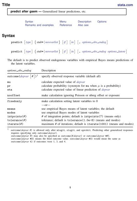
Syntax<br />
<strong>predict</strong> [ type ] { stub* | newvarlist } [ if ] [ in ] [ , options obs endog ]<br />
<strong>predict</strong> [ type ] { stub* | newvarlist } [ if ] [ in ] [ , options obs endog options latent ]<br />
The default is to <strong>predict</strong> observed endogenous variables with empirical Bayes means <strong>predict</strong>ions of<br />
the latent variables.<br />
options obs endog<br />
outcome(depvar [ # ] ) 1<br />
mu<br />
pr<br />
eta<br />
nooffset<br />
Description<br />
specify observed response variable (default all)<br />
calculate expected value of depvar<br />
calculate probability (synonym for mu when µ is a probability)<br />
calculate expected value of linear <strong>predict</strong>ion of depvar<br />
make calculation ignoring Poisson or nbreg offset or exposure<br />
fixedonly make calculation setting latent variables to 0<br />
—or—<br />
means<br />
use empirical Bayes means of latent variables; the default<br />
modes<br />
use empirical Bayes modes of latent variables<br />
intpoints(#) # of integration points; default is intpoints(7) (means only)<br />
tolerance(#) tolerance; default is tolerance(1.0e-8) (means and modes)<br />
iterate(#)<br />
maximum # of iterations; default is iterate(1001) (means and modes)<br />
1 outcome(depvar #) is allowed only <strong>after</strong> mlogit, ologit, and oprobit. Predicting other generalized responses<br />
requires specifying only outcome(depvar).<br />
outcome(depvar #) may also be specified as outcome(#.depvar) or outcome(depvar ##).<br />
outcome(depvar #3) means the third outcome value. outcome(depvar #3) would mean the same as<br />
outcome(depvar 4) if outcomes were 1, 3, and 4.<br />
1
2 <strong>predict</strong> <strong>after</strong> <strong>gsem</strong> — Generalized linear <strong>predict</strong>ions, etc.<br />
options latent<br />
∗ latent<br />
∗ latent(varlist)<br />
se(stub* | newvarlist)<br />
means<br />
modes<br />
intpoints(#)<br />
tolerance(#)<br />
iterate(#)<br />
Description<br />
calculate empirical Bayes <strong>predict</strong>ion of all latent variables<br />
calculate empirical Bayes <strong>predict</strong>ion of specified latent variables<br />
calculate standard errors<br />
use empirical Bayes means of latent variables; the default<br />
use empirical Bayes modes of latent variables<br />
# of integration points; default is intpoints(7) (means only)<br />
tolerance; default is tolerance(1.0e-8) (means and modes)<br />
maximum # of iterations; default is iterate(1001) (means and modes)<br />
∗ Either latent or latent() must be specified to obtain <strong>predict</strong>ions of latent variables.<br />
Menu<br />
Statistics > SEM (structural equation modeling) > Predictions<br />
Description<br />
<strong>predict</strong> is a standard postestimation command of <strong>Stata</strong>. This entry concerns use of <strong>predict</strong><br />
<strong>after</strong> <strong>gsem</strong>. See [SEM] <strong>predict</strong> <strong>after</strong> sem if you fit your model with sem.<br />
<strong>predict</strong> <strong>after</strong> <strong>gsem</strong> creates new variables containing observation-by-observation values of estimated<br />
observed response variables, linear <strong>predict</strong>ions of observed response variables, or endogenous or<br />
exogenous latent variables.<br />
or<br />
Out-of-sample <strong>predict</strong>ion is allowed in three cases:<br />
1. if the <strong>predict</strong>ion does not involve latent variables, or<br />
2. if the <strong>predict</strong>ion involves latent variables, directly or indirectly, option fixedonly is specified,<br />
or<br />
3. if the <strong>predict</strong>ion involves latent variables, directly or indirectly, the model is multilevel and<br />
no observational-level latent variables are involved.<br />
<strong>predict</strong> has two ways of specifying the name(s) of the variable(s) to be created:<br />
. <strong>predict</strong> stub*, . . .<br />
. <strong>predict</strong> firstname secondname . . . , . . .<br />
The first creates variables named stub1, stub2, . . . . The second creates variables named as you specify.<br />
We strongly recommend using the stub* syntax when creating multiple variables because you have<br />
no way of knowing the order in which to specify the individual variable names to correspond to the<br />
order in which <strong>predict</strong> will make the calculations. If you use stub*, the variables will be labeled<br />
and you can rename them.<br />
The second syntax is useful when creating one variable and you specify either outcome() or<br />
latent().
<strong>predict</strong> <strong>after</strong> <strong>gsem</strong> — Generalized linear <strong>predict</strong>ions, etc. 3<br />
Options<br />
outcome(depvar [ # ] ) and latent [ (varlist) ] determine what is to be calculated.<br />
neither specified<br />
outcome(depvar [#]) specified<br />
latent specified<br />
latent(varlist) specified<br />
<strong>predict</strong> all observed response variables<br />
<strong>predict</strong> specified observed response variable<br />
<strong>predict</strong> all latent variables<br />
<strong>predict</strong> specified latent variables<br />
If you are <strong>predict</strong>ing latent variables, both empirical Bayes means and modes are available; see<br />
options means, modes, intpoints(#), tolerance(#), and iterate(#) below.<br />
If you are <strong>predict</strong>ing observed response variables, you can obtain g −1 (x̂β) or x̂β; see options mu<br />
and eta below. Predictions can include latent variables or treat them as 0; see option fixedonly.<br />
If <strong>predict</strong>ions include latent variables, then just as when <strong>predict</strong>ing latent variables, both means and<br />
modes are available; see options means, modes, intpoints(#), tolerance(#), and iterate(#).<br />
mu and pr specify that g −1 (x̂β) be calculated, the inverse-link of the expected value of the linear<br />
<strong>predict</strong>ions. x by default contains <strong>predict</strong>ions of latent variables. pr is a synonym for mu if response<br />
variables are multinomial, ordinal, or Bernoulli. Otherwise, pr is not allowed.<br />
eta specifies that x̂β be calculated, the expected value of the linear <strong>predict</strong>ion. x by default contains<br />
<strong>predict</strong>ions of latent variables.<br />
fixedonly and nooffset are relevant only if observed response variables are being <strong>predict</strong>ed.<br />
fixedonly concerns <strong>predict</strong>ions of latent variables used in the <strong>predict</strong>ion of observed response<br />
variables. fixedonly specifies latent variables be treated as 0, and thus only the fixed-effects part<br />
of the model is used to produce the <strong>predict</strong>ions.<br />
nooffset is relevant only if option offset() or exposure() were specified at estimation time.<br />
nooffset specifies that offset() or exposure() be ignored, thus producing <strong>predict</strong>ions as if<br />
all subjects had equal exposure.<br />
means, modes, intpoints(#), tolerance(#), and iterate(#) specify what <strong>predict</strong>ions of the<br />
latent variables are to be calculated.<br />
means and modes specify that empirical Bayes means or modes be used. Means are the default.<br />
intpoints(#) specifies the number of numerical integration points and is relevant only in the<br />
calculation of empirical Bayes means. intpoints() defaults to the number of integration points<br />
specified at estimation time or to intpoints(7).<br />
tolerance(#) is relevant for the calculation of empirical Bayes means and modes. It specifies the<br />
convergence tolerance. It defaults to the value specified at estimation time with <strong>gsem</strong>’s adaptopts()<br />
or to tolerance(1e-8).<br />
iterate(#) is relevant for the calculation of empirical Bayes means and modes. It specifies the<br />
maximum number of iterations to be performed in the calculation of each integral. It defaults to<br />
the value specified at estimation time with <strong>gsem</strong>’s adaptopts() or to tolerance(1e-8).<br />
Remarks and examples<br />
See [SEM] intro 7, [SEM] example 28g, and [SEM] example 29g.<br />
stata.com
4 <strong>predict</strong> <strong>after</strong> <strong>gsem</strong> — Generalized linear <strong>predict</strong>ions, etc.<br />
Reference<br />
Skrondal, A., and S. Rabe-Hesketh. 2009. Prediction in multilevel generalized linear models. JRSSA 172: 659–687.<br />
Also see<br />
[SEM] <strong>gsem</strong> — Generalized structural equation model estimation command<br />
[SEM] <strong>gsem</strong> postestimation — Postestimation tools for <strong>gsem</strong><br />
[SEM] intro 7 — Postestimation tests and <strong>predict</strong>ions<br />
[SEM] example 28g — One-parameter logistic IRT (Rasch) model<br />
[SEM] example 29g — Two-parameter logistic IRT model<br />
[SEM] methods and formulas for <strong>gsem</strong> — Methods and formulas


