example 1 - Stata

Title
stata.com
example 1 — Single-factor measurement model
Description Remarks and examples Reference Also see
Description
The single-factor measurement model is demonstrated using the following data:
. use http://www.stata-press.com/data/r13/sem_1fmm
(single-factor measurement model)
. summarize
Variable Obs Mean Std. Dev. Min Max
x1 123 96.28455 14.16444 54 131
x2 123 97.28455 16.14764 64 135
x3 123 97.09756 15.10207 62 138
x4 123 690.9837 77.50737 481 885
. notes
_dta:
1. fictional data
2. Variables x1, x2, and x3 each contain a test score designed to measure X.
The test is scored to have mean 100.
3. Variable x4 is also designed to measure X, but designed to have mean 700.
See Single-factor measurement models in [SEM] intro 5 for background.
Remarks and examples
stata.com
Remarks are presented under the following headings:
Single-factor measurement model
Fitting the same model with gsem
Fitting the same model with the Builder
The measurement-error model interpretation
Single-factor measurement model
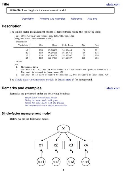
Below we fit the following model:
X
x1
x2
x3
x4
1
1
1
1
e.x1
e.x2
e.x3
e.x4
1

2 example 1 — Single-factor measurement model
. sem (x1 x2 x3 x4 |z| [95% Conf. Interval]
Measurement
x1

example 1 — Single-factor measurement model 3
2. The path coefficients for X->x1, X->x2, and X->x3 are 1 (constrained), 1.17, and 1.03. Meanwhile,
the path coefficient for X->x4 is 6.89. This is not unexpected; we at StataCorp generated this
data, and the true coefficients are 1, 1, 1, and 7.
3. A test for “model versus saturated” is reported at the bottom of the output; the χ 2 (2) statistic
is 1.78 and its significance level is 0.4111. We cannot reject the null hypothesis of this test.
This test is a goodness-of-fit test in badness-of-fit units; a significant result implies that there
may be missing paths in the model’s specification.
More mathematically, the null hypothesis of the test is that the fitted covariance matrix and mean
vector of the observed variables are equal to the matrix and vector observed in the population.
Fitting the same model with gsem
sem and gsem produce the same results for standard linear SEMs. We are going to demonstrate
that just this once.
. gsem (x1 x2 x3 x4 |z| [95% Conf. Interval]
x1

4 example 1 — Single-factor measurement model
Notes:
1. Results are virtually the same. Coefficients differ in the last digit; for instance, x2 SEM (structural equation modeling) > Model building and
estimation.
3. Create the measurement component for X.
Select the Add Measurement Component tool, , and then click in the diagram about one-third
of the way down from the top and slightly left of the center.
In the resulting dialog box,
a. change the Latent variable name to X;
b. select x1, x2, x3, and x4 by using the Measurement variables control;
c. select Down in the Measurement direction control;
d. click on OK.
If you wish, move the component by clicking on any variable and dragging it.
Notice that the constraints of 1 on the paths from the error terms to the observed measures are
implied, so we do not need to add these to our diagram.
4. Estimate.
Click on the Estimate button, , in the Standard Toolbar, and then click on OK in the resulting
SEM estimation options dialog box.
You can open a completed diagram in the Builder by typing
. webgetsem sem_1fmm

The measurement-error model interpretation
example 1 — Single-factor measurement model 5
As we pointed out in Using path diagrams to specify standard linear SEMs in [SEM] intro 2, if
we rename variable x4 to be y, we can reinterpret this measurement model as a measurement-error
model. In this interpretation, X is the unobserved true value. x1, x2, and x3 are each measurements
of X, but with error. Meanwhile, y (x4) is really something else entirely. Perhaps y is earnings, and
we believe
We are interested in β 4 , the effect of true X on y.
y = α 4 + β 4 X + e.y
If we were to go back to the data and type regress y x1, we would obtain an estimate of β 4 ,
but we would expect that estimate to be biased toward 0 because of the errors-in-variable problem.
The same applies for y on x2 and y on x3. If we do that, we obtain
β 4 based on regress y x1 4.09
β 4 based on regress y x2 3.71
β 4 based on regress y x3 3.70
In the sem output above, we have an estimate of β 4 with the bias washed away:
β 4 based on sem (y

6 example 1 — Single-factor measurement model
All the rnormal() functions remaining in our code have to do with the assumed normality of
the errors. The multiplicative and additive constants in the generation of X simply rescale the χ 2 (2)
variable to have mean 100 and standard deviation 10, which would not be important except for the
subsequent round() functions, which themselves were unnecessary except that we wanted to produce
a pretty dataset when we created the original sem 1fmm.dta.
In any case, if we rerun the commands with these data, we obtain
β 4 based on regress y x1 3.93
β 4 based on regress y x2 4.44
β 4 based on regress y x3 3.77
β 4 based on sem (y