

arima - Stata
arima - Stata
arima - Stata

You also want an ePaper? Increase the reach of your titles
YUMPU automatically turns print PDFs into web optimized ePapers that Google loves.
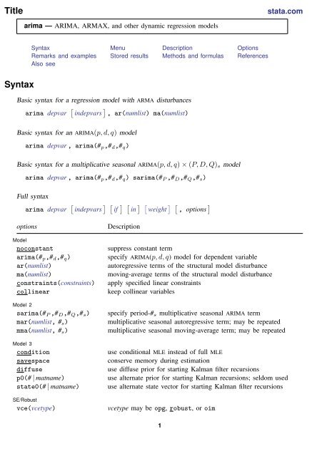
Title<br />
stata.com<br />
<strong>arima</strong> — ARIMA, ARMAX, and other dynamic regression models<br />
Syntax Menu Description Options<br />
Remarks and examples Stored results Methods and formulas References<br />
Also see<br />
Syntax<br />
Basic syntax for a regression model with ARMA disturbances<br />
<strong>arima</strong> depvar [ indepvars ] , ar(numlist) ma(numlist)<br />
Basic syntax for an ARIMA(p, d, q) model<br />
<strong>arima</strong> depvar , <strong>arima</strong>(# p ,# d ,# q )<br />
Basic syntax for a multiplicative seasonal ARIMA(p, d, q) × (P, D, Q) s model<br />
<strong>arima</strong> depvar , <strong>arima</strong>(# p ,# d ,# q ) s<strong>arima</strong>(# P ,# D ,# Q ,# s )<br />
Full syntax<br />
<strong>arima</strong> depvar [ indepvars ] [ if ] [ in ] [ weight ] [ , options ]<br />
options<br />
Model<br />
noconstant<br />
<strong>arima</strong>(# p ,# d ,# q )<br />
ar(numlist)<br />
ma(numlist)<br />
constraints(constraints)<br />
collinear<br />
Model 2<br />
s<strong>arima</strong>(# P ,# D ,# Q ,# s )<br />
mar(numlist, # s )<br />
mma(numlist, # s )<br />
Model 3<br />
condition<br />
savespace<br />
diffuse<br />
p0(# | matname)<br />
state0(# | matname)<br />
SE/Robust<br />
vce(vcetype)<br />
Description<br />
suppress constant term<br />
specify ARIMA(p, d, q) model for dependent variable<br />
autoregressive terms of the structural model disturbance<br />
moving-average terms of the structural model disturbance<br />
apply specified linear constraints<br />
keep collinear variables<br />
specify period-# s multiplicative seasonal ARIMA term<br />
multiplicative seasonal autoregressive term; may be repeated<br />
multiplicative seasonal moving-average term; may be repeated<br />
use conditional MLE instead of full MLE<br />
conserve memory during estimation<br />
use diffuse prior for starting Kalman filter recursions<br />
use alternate prior for starting Kalman recursions; seldom used<br />
use alternate state vector for starting Kalman filter recursions<br />
vcetype may be opg, robust, or oim<br />
1
2 <strong>arima</strong> — ARIMA, ARMAX, and other dynamic regression models<br />
Reporting<br />
level(#)<br />
detail<br />
nocnsreport<br />
display options<br />
Maximization<br />
maximize options<br />
coeflegend<br />
set confidence level; default is level(95)<br />
report list of gaps in time series<br />
do not display constraints<br />
control column formats, row spacing, and line width<br />
control the maximization process; seldom used<br />
display legend instead of statistics<br />
You must tsset your data before using <strong>arima</strong>; see [TS] tsset.<br />
depvar and indepvars may contain time-series operators; see [U] 11.4.4 Time-series varlists.<br />
by, fp, rolling, statsby, and xi are allowed; see [U] 11.1.10 Prefix commands.<br />
iweights are allowed; see [U] 11.1.6 weight.<br />
coeflegend does not appear in the dialog box.<br />
See [U] 20 Estimation and postestimation commands for more capabilities of estimation commands.<br />
Menu<br />
Statistics > Time series > ARIMA and ARMAX models<br />
Description<br />
<strong>arima</strong> fits univariate models with time-dependent disturbances. <strong>arima</strong> fits a model of depvar on<br />
indepvars where the disturbances are allowed to follow a linear autoregressive moving-average (ARMA)<br />
specification. The dependent and independent variables may be differenced or seasonally differenced<br />
to any degree. When independent variables are included in the specification, such models are often<br />
called ARMAX models; and when independent variables are not specified, they reduce to Box–Jenkins<br />
autoregressive integrated moving-average (ARIMA) models in the dependent variable. Multiplicative<br />
seasonal ARMAX and ARIMA models can also be fit. Missing data are allowed and are handled using<br />
the Kalman filter and methods suggested by Harvey (1989 and 1993); see Methods and formulas.<br />
In the full syntax, depvar is the variable being modeled, and the structural or regression part of<br />
the model is specified in indepvars. ar() and ma() specify the lags of autoregressive and movingaverage<br />
terms, respectively; and mar() and mma() specify the multiplicative seasonal autoregressive<br />
and moving-average terms, respectively.<br />
<strong>arima</strong> allows time-series operators in the dependent variable and independent variable lists, and<br />
making extensive use of these operators is often convenient; see [U] 11.4.4 Time-series varlists and<br />
[U] 13.9 Time-series operators for an extended discussion of time-series operators.<br />
Options<br />
<strong>arima</strong> typed without arguments redisplays the previous estimates.<br />
✄ <br />
✄ Model<br />
noconstant; see [R] estimation options.<br />
<strong>arima</strong>(# p ,# d ,# q ) is an alternative, shorthand notation for specifying models with ARMA disturbances.<br />
The dependent variable and any independent variables are differenced # d times, and 1 through # p<br />
lags of autocorrelations and 1 through # q lags of moving averages are included in the model. For<br />
example, the specification
<strong>arima</strong> — ARIMA, ARMAX, and other dynamic regression models 3<br />
✄<br />
✄<br />
. <strong>arima</strong> D.y, ar(1/2) ma(1/3)<br />
is equivalent to<br />
. <strong>arima</strong> y, <strong>arima</strong>(2,1,3)<br />
The latter is easier to write for simple ARMAX and ARIMA models, but if gaps in the AR or MA<br />
lags are to be modeled, or if different operators are to be applied to independent variables, the<br />
first syntax is required.<br />
ar(numlist) specifies the autoregressive terms of the structural model disturbance to be included in<br />
the model. For example, ar(1/3) specifies that lags of 1, 2, and 3 of the structural disturbance<br />
be included in the model; ar(1 4) specifies that lags 1 and 4 be included, perhaps to account for<br />
additive quarterly effects.<br />
If the model does not contain regressors, these terms can also be considered autoregressive terms<br />
for the dependent variable.<br />
ma(numlist) specifies the moving-average terms to be included in the model. These are the terms for<br />
the lagged innovations (white-noise disturbances).<br />
constraints(constraints), collinear; see [R] estimation options.<br />
If constraints are placed between structural model parameters and ARMA terms, the first few<br />
iterations may attempt steps into nonstationary areas. This process can be ignored if the final<br />
solution is well within the bounds of stationary solutions.<br />
✄<br />
Model 2<br />
<br />
s<strong>arima</strong>(# P ,# D ,# Q ,# s ) is an alternative, shorthand notation for specifying the multiplicative seasonal<br />
components of models with ARMA disturbances. The dependent variable and any independent<br />
variables are lag-# s seasonally differenced # D times, and 1 through # P seasonal lags of autoregressive<br />
terms and 1 through # Q seasonal lags of moving-average terms are included in the model. For<br />
example, the specification<br />
. <strong>arima</strong> DS12.y, ar(1/2) ma(1/3) mar(1/2,12) mma(1/2,12)<br />
is equivalent to<br />
. <strong>arima</strong> y, <strong>arima</strong>(2,1,3) s<strong>arima</strong>(2,1,2,12)<br />
mar(numlist, # s ) specifies the lag-# s multiplicative seasonal autoregressive terms. For example,<br />
mar(1/2,12) requests that the first two lag-12 multiplicative seasonal autoregressive terms be<br />
included in the model.<br />
mma(numlist, # s ) specified the lag-# s multiplicative seasonal moving-average terms. For example,<br />
mma(1 3,12) requests that the first and third (but not the second) lag-12 multiplicative seasonal<br />
moving-average terms be included in the model.<br />
✄<br />
Model 3<br />
<br />
condition specifies that conditional, rather than full, maximum likelihood estimates be produced.<br />
The presample values for ɛ t and µ t are taken to be their expected value of zero, and the estimate<br />
of the variance of ɛ t is taken to be constant over the entire sample; see Hamilton (1994, 132).<br />
This estimation method is not appropriate for nonstationary series but may be preferable for long<br />
series or for models that have one or more long AR or MA lags. diffuse, p0(), and state0()<br />
have no meaning for models fit from the conditional likelihood and may not be specified with<br />
condition.
4 <strong>arima</strong> — ARIMA, ARMAX, and other dynamic regression models<br />
If the series is long and stationary and the underlying data-generating process does not have a long<br />
memory, estimates will be similar, whether estimated by unconditional maximum likelihood (the<br />
default), conditional maximum likelihood (condition), or maximum likelihood from a diffuse<br />
prior (diffuse).<br />
In small samples, however, results of conditional and unconditional maximum likelihood may<br />
differ substantially; see Ansley and Newbold (1980). Whereas the default unconditional maximum<br />
likelihood estimates make the most use of sample information when all the assumptions of the model<br />
are met, Harvey (1989) and Ansley and Kohn (1985) argue for diffuse priors often, particularly in<br />
ARIMA models corresponding to an underlying structural model.<br />
The condition or diffuse options may also be preferred when the model contains one or more<br />
long AR or MA lags; this avoids inverting potentially large matrices (see diffuse below).<br />
When condition is specified, estimation is performed by the arch command (see [TS] arch),<br />
and more control of the estimation process can be obtained using arch directly.<br />
condition cannot be specified if the model contains any multiplicative seasonal terms.<br />
savespace specifies that memory use be conserved by retaining only those variables required for<br />
estimation. The original dataset is restored after estimation. This option is rarely used and should<br />
be used only if there is not enough space to fit a model without the option. However, <strong>arima</strong><br />
requires considerably more temporary storage during estimation than most estimation commands<br />
in <strong>Stata</strong>.<br />
diffuse specifies that a diffuse prior (see Harvey 1989 or 1993) be used as a starting point for the<br />
Kalman filter recursions. Using diffuse, nonstationary models may be fit with <strong>arima</strong> (see the<br />
p0() option below; diffuse is equivalent to specifying p0(1e9)).<br />
By default, <strong>arima</strong> uses the unconditional expected value of the state vector ξ t (see Methods and<br />
formulas) and the mean squared error (MSE) of the state vector to initialize the filter. When the<br />
process is stationary, this corresponds to the expected value and expected variance of a random draw<br />
from the state vector and produces unconditional maximum likelihood estimates of the parameters.<br />
When the process is not stationary, however, this default is not appropriate, and the unconditional<br />
MSE cannot be computed. For a nonstationary process, another starting point must be used for the<br />
recursions.<br />
In the absence of nonsample or presample information, diffuse may be specified to start the<br />
recursions from a state vector of zero and a state MSE matrix corresponding to an effectively<br />
infinite variance on this initial state. This method amounts to an uninformative and improper prior<br />
that is updated to a proper MSE as data from the sample become available; see Harvey (1989).<br />
Nonstationary models may also correspond to models with infinite variance given a particular<br />
specification. This and other problems with nonstationary series make convergence difficult and<br />
sometimes impossible.<br />
diffuse can also be useful if a model contains one or more long AR or MA lags. Computation<br />
of the unconditional MSE of the state vector (see Methods and formulas) requires construction<br />
and inversion of a square matrix that is of dimension {max(p, q + 1)} 2 , where p and q are the<br />
maximum AR and MA lags, respectively. If q = 27, for example, we would require a 784-by-784<br />
matrix. Estimation with diffuse does not require this matrix.<br />
For large samples, there is little difference between using the default starting point and the diffuse<br />
starting point. Unless the series has a long memory, the initial conditions affect the likelihood of<br />
only the first few observations.
<strong>arima</strong> — ARIMA, ARMAX, and other dynamic regression models 5<br />
p0(# | matname) is a rarely specified option that can be used for nonstationary series or when an<br />
alternate prior for starting the Kalman recursions is desired (see diffuse above for a discussion<br />
of the default starting point and Methods and formulas for background).<br />
matname specifies a matrix to be used as the MSE of the state vector for starting the Kalman filter<br />
recursions—P 1|0 . Instead, one number, #, may be supplied, and the MSE of the initial state vector<br />
P 1|0 will have this number on its diagonal and all off-diagonal values set to zero.<br />
This option may be used with nonstationary series to specify a larger or smaller diagonal for P 1|0<br />
than that supplied by diffuse. It may also be used with state0() when you believe that you<br />
have a better prior for the initial state vector and its MSE.<br />
state0(# | matname) is a rarely used option that specifies an alternate initial state vector, ξ 1|0 (see<br />
Methods and formulas), for starting the Kalman filter recursions. If # is specified, all elements of<br />
the vector are taken to be #. The default initial state vector is state0(0).<br />
✄<br />
✄ <br />
SE/Robust<br />
<br />
vce(vcetype) specifies the type of standard error reported, which includes types that are robust to<br />
some kinds of misspecification (robust) and that are derived from asymptotic theory (oim, opg);<br />
see [R] vce option.<br />
For state-space models in general and ARMAX and ARIMA models in particular, the robust or<br />
quasi–maximum likelihood estimates (QMLEs) of variance are robust to symmetric nonnormality<br />
in the disturbances, including, as a special case, heteroskedasticity. The robust variance estimates<br />
are not generally robust to functional misspecification of the structural or ARMA components of<br />
the model; see Hamilton (1994, 389) for a brief discussion.<br />
✄ <br />
✄ Reporting<br />
level(#); see [R] estimation options.<br />
✄<br />
detail specifies that a detailed list of any gaps in the series be reported, including gaps due to<br />
missing observations or missing data for the dependent variable or independent variables.<br />
nocnsreport; see [R] estimation options.<br />
display options: vsquish, cformat(% fmt), pformat(% fmt), sformat(% fmt), and nolstretch;<br />
see [R] estimation options.<br />
✄<br />
Maximization<br />
<br />
maximize options: difficult, technique(algorithm spec), iterate(#), [ no ] log, trace,<br />
gradient, showstep, hessian, showtolerance, tolerance(#), ltolerance(#),<br />
nrtolerance(#), gtolerance(#), nonrtolerance(#), and from(init specs); see [R] maximize<br />
for all options except gtolerance(), and see below for information on gtolerance().<br />
These options are sometimes more important for ARIMA models than most maximum likelihood<br />
models because of potential convergence problems with ARIMA models, particularly if the specified<br />
model and the sample data imply a nonstationary model.<br />
Several alternate optimization methods, such as Berndt–Hall–Hall–Hausman (BHHH) and Broyden–<br />
Fletcher–Goldfarb–Shanno (BFGS), are provided for ARIMA models. Although ARIMA models are<br />
not as difficult to optimize as ARCH models, their likelihoods are nevertheless generally not quadratic<br />
and often pose optimization difficulties; this is particularly true if a model is nonstationary or<br />
nearly nonstationary. Because each method approaches optimization differently, some problems<br />
can be successfully optimized by an alternate method when one method fails.<br />
Setting technique() to something other than the default or BHHH changes the vcetype to vce(oim).
6 <strong>arima</strong> — ARIMA, ARMAX, and other dynamic regression models<br />
The following options are all related to maximization and are either particularly important in fitting<br />
ARIMA models or not available for most other estimators.<br />
technique(algorithm spec) specifies the optimization technique to use to maximize the<br />
likelihood function.<br />
technique(bhhh) specifies the Berndt–Hall–Hall–Hausman (BHHH) algorithm.<br />
technique(dfp) specifies the Davidon–Fletcher–Powell (DFP) algorithm.<br />
technique(bfgs) specifies the Broyden–Fletcher–Goldfarb–Shanno (BFGS) algorithm.<br />
technique(nr) specifies <strong>Stata</strong>’s modified Newton–Raphson (NR) algorithm.<br />
You can specify multiple optimization methods. For example,<br />
technique(bhhh 10 nr 20)<br />
requests that the optimizer perform 10 BHHH iterations, switch to Newton–Raphson for 20<br />
iterations, switch back to BHHH for 10 more iterations, and so on.<br />
The default for <strong>arima</strong> is technique(bhhh 5 bfgs 10).<br />
gtolerance(#) specifies the tolerance for the gradient relative to the coefficients. When<br />
|g i b i | ≤ gtolerance() for all parameters b i and the corresponding elements of the<br />
gradient g i , the gradient tolerance criterion is met. The default gradient tolerance for <strong>arima</strong><br />
is gtolerance(.05).<br />
gtolerance(999) may be specified to disable the gradient criterion. If the optimizer becomes<br />
stuck with repeated “(backed up)” messages, the gradient probably still contains substantial<br />
values, but an uphill direction cannot be found for the likelihood. With this option, results can<br />
often be obtained, but whether the global maximum likelihood has been found is unclear.<br />
When the maximization is not going well, it is also possible to set the maximum number of<br />
iterations (see [R] maximize) to the point where the optimizer appears to be stuck and to inspect<br />
the estimation results at that point.<br />
from(init specs) allows you to set the starting values of the model coefficients; see [R] maximize<br />
for a general discussion and syntax options.<br />
The standard syntax for from() accepts a matrix, a list of values, or coefficient name value<br />
pairs; see [R] maximize. <strong>arima</strong> also accepts from(armab0), which sets the starting value for<br />
all ARMA parameters in the model to zero prior to optimization.<br />
ARIMA models may be sensitive to initial conditions and may have coefficient values that<br />
correspond to local maximums. The default starting values for <strong>arima</strong> are generally good,<br />
particularly in large samples for stationary series.<br />
The following option is available with <strong>arima</strong> but is not shown in the dialog box:<br />
coeflegend; see [R] estimation options.
<strong>arima</strong> — ARIMA, ARMAX, and other dynamic regression models 7<br />
Remarks and examples<br />
Remarks are presented under the following headings:<br />
Introduction<br />
ARIMA models<br />
Multiplicative seasonal ARIMA models<br />
ARMAX models<br />
Dynamic forecasting<br />
Video example<br />
stata.com<br />
Introduction<br />
<strong>arima</strong> fits both standard ARIMA models that are autoregressive in the dependent variable and<br />
structural models with ARMA disturbances. Good introductions to the former models can be found in<br />
Box, Jenkins, and Reinsel (2008); Hamilton (1994); Harvey (1993); Newton (1988); Diggle (1990);<br />
and many others. The latter models are developed fully in Hamilton (1994) and Harvey (1989), both of<br />
which provide extensive treatment of the Kalman filter (Kalman 1960) and the state-space form used<br />
by <strong>arima</strong> to fit the models. Becketti (2013) discusses ARIMA models and <strong>Stata</strong>’s <strong>arima</strong> command,<br />
and he devotes an entire chapter explaining how the principles of ARIMA models are applied to real<br />
datasets in practice.<br />
Consider a first-order autoregressive moving-average process. Then <strong>arima</strong> estimates all the parameters<br />
in the model<br />
where<br />
ρ<br />
θ<br />
ɛ t<br />
y t = x t β + µ t<br />
structural equation<br />
µ t = ρµ t−1 + θɛ t−1 + ɛ t disturbance, ARMA(1, 1)<br />
is the first-order autocorrelation parameter<br />
is the first-order moving-average parameter<br />
∼ i.i.d. N(0, σ 2 ), meaning that ɛ t is a white-noise disturbance<br />
You can combine the two equations and write a general ARMA(p, q) in the disturbances process as<br />
y t = x t β + ρ 1 (y t−1 − x t−1 β) + ρ 2 (y t−2 − x t−2 β) + · · · + ρ p (y t−p − x t−p β)<br />
+ θ 1 ɛ t−1 + θ 2 ɛ t−2 + · · · + θ q ɛ t−q + ɛ t<br />
It is also common to write the general form of the ARMA model more succinctly using lag operator<br />
notation as<br />
ρ(L p )(y t − x t β) = θ(L q )ɛ t ARMA(p, q)<br />
where<br />
ρ(L p ) = 1 − ρ 1 L − ρ 2 L 2 − · · · − ρ p L p<br />
θ(L q ) = 1 + θ 1 L + θ 2 L 2 + · · · + θ q L q<br />
and L j y t = y t−j .<br />
For stationary series, full or unconditional maximum likelihood estimates are obtained via the<br />
Kalman filter. For nonstationary series, if some prior information is available, you can specify initial<br />
values for the filter by using state0() and p0() as suggested by Hamilton (1994) or assume an<br />
uninformative prior by using the diffuse option as suggested by Harvey (1989).
8 <strong>arima</strong> — ARIMA, ARMAX, and other dynamic regression models<br />
ARIMA models<br />
Pure ARIMA models without a structural component do not have regressors and are often written<br />
as autoregressions in the dependent variable, rather than autoregressions in the disturbances from a<br />
structural equation. For example, an ARMA(1, 1) model can be written as<br />
y t = α + ρy t−1 + θɛ t−1 + ɛ t<br />
(1a)<br />
Other than a scale factor for the constant term α, these models are equivalent to the ARMA in the<br />
disturbances formulation estimated by <strong>arima</strong>, though the latter are more flexible and allow a wider<br />
class of models.<br />
To see this effect, replace x t β in the structural equation above with a constant term β 0 so that<br />
y t = β 0 + µ t<br />
= β 0 + ρµ t−1 + θɛ t−1 + ɛ t<br />
= β 0 + ρ(y t−1 − β 0 ) + θɛ t−1 + ɛ t<br />
= (1 − ρ)β 0 + ρy t−1 + θɛ t−1 + ɛ t (1b)<br />
Equations (1a) and (1b) are equivalent, with α = (1 − ρ)β 0 , so whether we consider an ARIMA model<br />
as autoregressive in the dependent variable or disturbances is immaterial. Our illustration can easily<br />
be extended from the ARMA(1, 1) case to the general ARIMA(p, d, q) case.<br />
Example 1: ARIMA model<br />
Enders (2004, 87–93) considers an ARIMA model of the U.S. Wholesale Price Index (WPI)<br />
using quarterly data over the period 1960q1 through 1990q4. The simplest ARIMA model that includes<br />
differencing and both autoregressive and moving-average components is the ARIMA(1,1,1) specification.<br />
We can fit this model with <strong>arima</strong> by typing
<strong>arima</strong> — ARIMA, ARMAX, and other dynamic regression models 9<br />
. use http://www.stata-press.com/data/r13/wpi1<br />
. <strong>arima</strong> wpi, <strong>arima</strong>(1,1,1)<br />
(setting optimization to BHHH)<br />
Iteration 0: log likelihood = -139.80133<br />
Iteration 1: log likelihood = -135.6278<br />
Iteration 2: log likelihood = -135.41838<br />
Iteration 3: log likelihood = -135.36691<br />
Iteration 4: log likelihood = -135.35892<br />
(switching optimization to BFGS)<br />
Iteration 5: log likelihood = -135.35471<br />
Iteration 6: log likelihood = -135.35135<br />
Iteration 7: log likelihood = -135.35132<br />
Iteration 8: log likelihood = -135.35131<br />
ARIMA regression<br />
Sample: 1960q2 - 1990q4 Number of obs = 123<br />
Wald chi2(2) = 310.64<br />
Log likelihood = -135.3513 Prob > chi2 = 0.0000<br />
OPG<br />
D.wpi Coef. Std. Err. z P>|z| [95% Conf. Interval]<br />
wpi<br />
ARMA<br />
_cons .7498197 .3340968 2.24 0.025 .0950019 1.404637<br />
ar<br />
L1. .8742288 .0545435 16.03 0.000 .7673256 .981132<br />
ma<br />
L1. -.4120458 .1000284 -4.12 0.000 -.6080979 -.2159938<br />
/sigma .7250436 .0368065 19.70 0.000 .6529042 .7971829<br />
Note: The test of the variance against zero is one sided, and the two-sided<br />
confidence interval is truncated at zero.<br />
Examining the estimation results, we see that the AR(1) coefficient is 0.874, the MA(1) coefficient<br />
is −0.412, and both are highly significant. The estimated standard deviation of the white-noise<br />
disturbance ɛ is 0.725.<br />
This model also could have been fit by typing<br />
. <strong>arima</strong> D.wpi, ar(1) ma(1)<br />
The D. placed in front of the dependent variable wpi is the <strong>Stata</strong> time-series operator for differencing.<br />
Thus we would be modeling the first difference in WPI from the second quarter of 1960 through<br />
the fourth quarter of 1990 because the first observation is lost because of differencing. This second<br />
syntax allows a richer choice of models.<br />
Example 2: ARIMA model with additive seasonal effects<br />
After examining first-differences of WPI, Enders chose a model of differences in the natural<br />
logarithms to stabilize the variance in the differenced series. The raw data and first-difference of the<br />
logarithms are graphed below.
10 <strong>arima</strong> — ARIMA, ARMAX, and other dynamic regression models<br />
25 50 75 100 125<br />
US Wholesale Price Index<br />
1960q1 1970q1 1980q1 1990q1<br />
t<br />
−.04 −.02 0 .02 .04 .06 .08<br />
US Wholesale Price Index −− difference of logs<br />
1960q1 1970q1 1980q1 1990q1<br />
t<br />
On the basis of the autocorrelations, partial autocorrelations (see graphs below), and the results of<br />
preliminary estimations, Enders identified an ARMA model in the log-differenced series.<br />
. ac D.ln_wpi, ylabels(-.4(.2).6)<br />
. pac D.ln_wpi, ylabels(-.4(.2).6)<br />
Autocorrelations of D.ln_wpi<br />
−0.40 −0.20 0.00 0.20 0.40 0.60<br />
0 10 20 30 40<br />
Lag<br />
Bartlett’s formula for MA(q) 95% confidence bands<br />
Partial autocorrelations of D.ln_wpi<br />
−0.40 −0.20 0.00 0.20 0.40 0.60<br />
0 10 20 30 40<br />
Lag<br />
95% Confidence bands [se = 1/sqrt(n)]<br />
In addition to an autoregressive term and an MA(1) term, an MA(4) term is included to account<br />
for a remaining quarterly effect. Thus the model to be fit is<br />
∆ ln(wpi t ) = β 0 + ρ 1 {∆ ln(wpi t−1 ) − β 0 } + θ 1 ɛ t−1 + θ 4 ɛ t−4 + ɛ t
<strong>arima</strong> — ARIMA, ARMAX, and other dynamic regression models 11<br />
We can fit this model with <strong>arima</strong> and <strong>Stata</strong>’s standard difference operator:<br />
. <strong>arima</strong> D.ln_wpi, ar(1) ma(1 4)<br />
(setting optimization to BHHH)<br />
Iteration 0: log likelihood = 382.67447<br />
Iteration 1: log likelihood = 384.80754<br />
Iteration 2: log likelihood = 384.84749<br />
Iteration 3: log likelihood = 385.39213<br />
Iteration 4: log likelihood = 385.40983<br />
(switching optimization to BFGS)<br />
Iteration 5: log likelihood = 385.9021<br />
Iteration 6: log likelihood = 385.95646<br />
Iteration 7: log likelihood = 386.02979<br />
Iteration 8: log likelihood = 386.03326<br />
Iteration 9: log likelihood = 386.03354<br />
Iteration 10: log likelihood = 386.03357<br />
ARIMA regression<br />
Sample: 1960q2 - 1990q4 Number of obs = 123<br />
Wald chi2(3) = 333.60<br />
Log likelihood = 386.0336 Prob > chi2 = 0.0000<br />
OPG<br />
D.ln_wpi Coef. Std. Err. z P>|z| [95% Conf. Interval]<br />
ln_wpi<br />
ARMA<br />
_cons .0110493 .0048349 2.29 0.022 .0015731 .0205255<br />
ar<br />
L1. .7806991 .0944946 8.26 0.000 .5954931 .965905<br />
ma<br />
L1. -.3990039 .1258753 -3.17 0.002 -.6457149 -.1522928<br />
L4. .3090813 .1200945 2.57 0.010 .0737003 .5444622<br />
/sigma .0104394 .0004702 22.20 0.000 .0095178 .0113609<br />
Note: The test of the variance against zero is one sided, and the two-sided<br />
confidence interval is truncated at zero.<br />
In this final specification, the log-differenced series is still highly autocorrelated at a level of 0.781,<br />
though innovations have a negative impact in the ensuing quarter (−0.399) and a positive seasonal<br />
impact of 0.309 in the following year.<br />
Technical note<br />
In one way, the results differ from most of <strong>Stata</strong>’s estimation commands: the standard error of<br />
the coefficients is reported as OPG Std. Err. The default standard errors and covariance matrix<br />
for <strong>arima</strong> estimates are derived from the outer product of gradients (OPG). This is one of three<br />
asymptotically equivalent methods of estimating the covariance matrix of the coefficients (only two of<br />
which are usually tractable to derive). Discussions and derivations of all three estimates can be found<br />
in Davidson and MacKinnon (1993), Greene (2012), and Hamilton (1994). Bollerslev, Engle, and<br />
Nelson (1994) suggest that the OPG estimates are more numerically stable in time-series regressions<br />
when the likelihood and its derivatives depend on recursive computations, which is certainly the case<br />
for the Kalman filter. To date, we have found no numerical instabilities in either estimate of the<br />
covariance matrix—subject to the stability and convergence of the overall model.
12 <strong>arima</strong> — ARIMA, ARMAX, and other dynamic regression models<br />
Most of <strong>Stata</strong>’s estimation commands provide covariance estimates derived from the Hessian of<br />
the likelihood function. These alternate estimates can also be obtained from <strong>arima</strong> by specifying the<br />
vce(oim) option.<br />
Multiplicative seasonal ARIMA models<br />
Many time series exhibit a periodic seasonal component, and a seasonal ARIMA model, often<br />
abbreviated SARIMA, can then be used. For example, monthly sales data for air conditioners have a<br />
strong seasonal component, with sales high in the summer months and low in the winter months.<br />
In the previous example, we accounted for quarterly effects by fitting the model<br />
(1 − ρ 1 L){∆ ln(wpi t ) − β 0 } = (1 + θ 1 L + θ 4 L 4 )ɛ t<br />
This is an additive seasonal ARIMA model, in the sense that the first- and fourth-order MA terms work<br />
additively: (1 + θ 1 L + θ 4 L 4 ).<br />
Another way to handle the quarterly effect would be to fit a multiplicative seasonal ARIMA model.<br />
A multiplicative SARIMA model of order (1, 1, 1) × (0, 0, 1) 4 for the ln(wpi t ) series is<br />
or, upon expanding terms,<br />
(1 − ρ 1 L){∆ ln(wpi t ) − β 0 } = (1 + θ 1 L)(1 + θ 4,1 L 4 )ɛ t<br />
∆ ln(wpi t ) = β 0 + ρ 1 {∆ ln(wpi t ) − β 0 } + θ 1 ɛ t−1 + θ 4,1 ɛ t−4 + θ 1 θ 4,1 ɛ t−5 + ɛ t (2)<br />
In the notation (1, 1, 1) × (0, 0, 1) 4 , the (1, 1, 1) means that there is one nonseasonal autoregressive<br />
term (1 − ρ 1 L) and one nonseasonal moving-average term (1 + θ 1 L) and that the time series is<br />
first-differenced one time. The (0, 0, 1) 4 indicates that there is no lag-4 seasonal autoregressive term,<br />
that there is one lag-4 seasonal moving-average term (1 + θ 4,1 L 4 ), and that the series is seasonally<br />
differenced zero times. This is known as a multiplicative SARIMA model because the nonseasonal<br />
and seasonal factors work multiplicatively: (1 + θ 1 L)(1 + θ 4,1 L 4 ). Multiplying the terms imposes<br />
nonlinear constraints on the parameters of the fifth-order lagged values; <strong>arima</strong> imposes these constraints<br />
automatically.<br />
To further clarify the notation, consider a (2, 1, 1) × (1, 1, 2) 4 multiplicative SARIMA model:<br />
(1 − ρ 1 L − ρ 2 L 2 )(1 − ρ 4,1 L 4 )∆∆ 4 z t = (1 + θ 1 L)(1 + θ 4,1 L 4 + θ 4,2 L 8 )ɛ t (3)<br />
where ∆ denotes the difference operator ∆y t = y t − y t−1 and ∆ s denotes the lag-s seasonal<br />
difference operator ∆ s y t = y t − y t−s . Expanding (3), we have<br />
˜z t = ρ 1˜z t−1 + ρ 2˜z t−2 + ρ 4,1˜z t−4 − ρ 1 ρ 4,1˜z t−5 − ρ 2 ρ 4,1˜z t−6<br />
+ θ 1 ɛ t−1 + θ 4,1 ɛ t−4 + θ 1 θ 4,1 ɛ t−5 + θ 4,2 ɛ t−8 + θ 1 θ 4,2 ɛ t−9 + ɛ t<br />
where<br />
˜z t = ∆∆ 4 z t = ∆(z t − z t−4 ) = z t − z t−1 − (z t−4 − z t−5 )<br />
and z t = y t − x t β if regressors are included in the model, z t = y t − β 0 if just a constant term is<br />
included, and z t = y t otherwise.
<strong>arima</strong> — ARIMA, ARMAX, and other dynamic regression models 13<br />
More generally, a (p, d, q) × (P, D, Q) s multiplicative SARIMA model is<br />
ρ(L p )ρ s (L P )∆ d ∆ D s z t = θ(L q )θ s (L Q )ɛ t<br />
where<br />
ρ s (L P ) = (1 − ρ s,1 L s − ρ s,2 L 2s − · · · − ρ s,P L P s )<br />
θ s (L Q ) = (1 + θ s,1 L s + θ s,2 L 2s + · · · + θ s,Q L Qs )<br />
ρ(L p ) and θ(L q ) were defined previously, ∆ d means apply the ∆ operator d times, and similarly<br />
for ∆ D s . Typically, d and D will be 0 or 1; and p, q, P , and Q will seldom be more than 2 or 3. s<br />
will typically be 4 for quarterly data and 12 for monthly data. In fact, the model can be extended to<br />
include both monthly and quarterly seasonal factors, as we explain below.<br />
If a plot of the data suggests that the seasonal effect is proportional to the mean of the series, then<br />
the seasonal effect is probably multiplicative and a multiplicative SARIMA model may be appropriate.<br />
Box, Jenkins, and Reinsel (2008, sec. 9.3.1) suggest starting with a multiplicative SARIMA model with<br />
any data that exhibit seasonal patterns and then exploring nonmultiplicative SARIMA models if the<br />
multiplicative models do not fit the data well. On the other hand, Chatfield (2004, 14) suggests that<br />
taking the logarithm of the series will make the seasonal effect additive, in which case an additive<br />
SARIMA model as fit in the previous example would be appropriate. In short, the analyst should<br />
probably try both additive and multiplicative SARIMA models to see which provides better fits and<br />
forecasts.<br />
Unless diffuse is used, <strong>arima</strong> must create square matrices of dimension {max(p, q +1)} 2 , where<br />
p and q are the maximum AR and MA lags, respectively; and the inclusion of long seasonal terms can<br />
make this dimension rather large. For example, with monthly data, you might fit a (0, 1, 1)×(0, 1, 2) 12<br />
SARIMA model. The maximum MA lag is 2 × 12 + 1 = 25, requiring a matrix with 26 2 = 676 rows<br />
and columns.<br />
Example 3: Multiplicative SARIMA model<br />
One of the most common multiplicative SARIMA specifications is the (0, 1, 1)×(0, 1, 1) 12 “airline”<br />
model of Box, Jenkins, and Reinsel (2008, sec. 9.2). The dataset airline.dta contains monthly<br />
international airline passenger data from January 1949 through December 1960. After first- and<br />
seasonally differencing the data, we do not suspect the presence of a trend component, so we use the<br />
noconstant option with <strong>arima</strong>:
14 <strong>arima</strong> — ARIMA, ARMAX, and other dynamic regression models<br />
. use http://www.stata-press.com/data/r13/air2<br />
(TIMESLAB: Airline passengers)<br />
. generate lnair = ln(air)<br />
. <strong>arima</strong> lnair, <strong>arima</strong>(0,1,1) s<strong>arima</strong>(0,1,1,12) noconstant<br />
(setting optimization to BHHH)<br />
Iteration 0: log likelihood = 223.8437<br />
Iteration 1: log likelihood = 239.80405<br />
(output omitted )<br />
Iteration 8: log likelihood = 244.69651<br />
ARIMA regression<br />
Sample: 14 - 144 Number of obs = 131<br />
Wald chi2(2) = 84.53<br />
Log likelihood = 244.6965 Prob > chi2 = 0.0000<br />
OPG<br />
DS12.lnair Coef. Std. Err. z P>|z| [95% Conf. Interval]<br />
ARMA<br />
ARMA12<br />
ma<br />
L1. -.4018324 .0730307 -5.50 0.000 -.5449698 -.2586949<br />
ma<br />
L1. -.5569342 .0963129 -5.78 0.000 -.745704 -.3681644<br />
/sigma .0367167 .0020132 18.24 0.000 .0327708 .0406625<br />
Note: The test of the variance against zero is one sided, and the two-sided<br />
confidence interval is truncated at zero.<br />
Thus our model of the monthly number of international airline passengers is<br />
∆∆ 12 lnair t = −0.402ɛ t−1 − 0.557ɛ t−12 + 0.224ɛ t−13 + ɛ t<br />
̂σ = 0.037<br />
In (2), for example, the coefficient on ɛ t−13 is the product of the coefficients on the ɛ t−1 and ɛ t−12<br />
terms (0.224 ≈ −0.402 × −0.557). <strong>arima</strong> labeled the dependent variable DS12.lnair to indicate<br />
that it has applied the difference operator ∆ and the lag-12 seasonal difference operator ∆ 12 to<br />
lnair; see [U] 11.4.4 Time-series varlists for more information.<br />
We could have fit this model by typing<br />
. <strong>arima</strong> DS12.lnair, ma(1) mma(1, 12) noconstant<br />
For simple multiplicative models, using the s<strong>arima</strong>() option is easier, though this second syntax<br />
allows us to incorporate more complicated seasonal terms.<br />
The mar() and mma() options can be repeated, allowing us to control for multiple seasonal<br />
patterns. For example, we may have monthly sales data that exhibit a quarterly pattern as businesses<br />
purchase our product at the beginning of calendar quarters when new funds are budgeted, and our<br />
product is purchased more frequently in a few months of the year than in most others, even after we<br />
control for quarterly fluctuations. Thus we might choose to fit the model<br />
(1−ρL)(1−ρ 4,1 L 4 )(1−ρ 12,1 L 12 )(∆∆ 4 ∆ 12 sales t −β 0 ) = (1+θL)(1+θ 4,1 L 4 )(1+θ 12,1 L 12 )ɛ t
<strong>arima</strong> — ARIMA, ARMAX, and other dynamic regression models 15<br />
Although this model looks rather complicated, estimating it using <strong>arima</strong> is straightforward:<br />
. <strong>arima</strong> DS4S12.sales, ar(1) mar(1, 4) mar(1, 12) ma(1) mma(1, 4) mma(1, 12)<br />
If we instead wanted to include two lags in the lag-4 seasonal AR term and the first and third (but<br />
not the second) term in the lag-12 seasonal MA term, we would type<br />
. <strong>arima</strong> DS4S12.sales, ar(1) mar(1 2, 4) mar(1, 12) ma(1) mma(1, 4) mma(1 3, 12)<br />
However, models with multiple seasonal terms can be difficult to fit. Usually, one seasonal factor<br />
with just one or two AR or MA terms is adequate.<br />
ARMAX models<br />
Thus far all our examples have been pure ARIMA models in which the dependent variable was<br />
modeled solely as a function of its past values and disturbances. Also, <strong>arima</strong> can fit ARMAX models,<br />
which model the dependent variable in terms of a linear combination of independent variables, as<br />
well as an ARMA disturbance process. The prais command (see [TS] prais), for example, allows<br />
you to control for only AR(1) disturbances, whereas <strong>arima</strong> allows you to control for a much richer<br />
dynamic error structure. <strong>arima</strong> allows for both nonseasonal and seasonal ARMA components in the<br />
disturbances.<br />
Example 4: ARMAX model<br />
For a simple example of a model including covariates, we can estimate an update of Friedman and<br />
Meiselman’s (1963) equation representing the quantity theory of money. They postulate a straightforward<br />
relationship between personal-consumption expenditures (consump) and the money supply<br />
as measured by M2 (m2).<br />
consump t = β 0 + β 1 m2 t + µ t<br />
Friedman and Meiselman fit the model over a period ending in 1956; we will refit the model over<br />
the period 1959q1 through 1981q4. We restrict our attention to the period prior to 1982 because the<br />
Federal Reserve manipulated the money supply extensively in the later 1980s to control inflation, and<br />
the relationship between consumption and the money supply becomes much more complex during<br />
the later part of the decade.<br />
To demonstrate <strong>arima</strong>, we will include both an autoregressive term and a moving-average term for<br />
the disturbances in the model; the original estimates included neither. Thus we model the disturbance<br />
of the structural equation as<br />
µ t = ρµ t−1 + θɛ t−1 + ɛ t<br />
As per the original authors, the relationship is estimated on seasonally adjusted data, so there is no<br />
need to include seasonal effects explicitly. Obtaining seasonally unadjusted data and simultaneously<br />
modeling the structural and seasonal effects might be preferable.<br />
We will restrict the estimation to the desired sample by using the tin() function in an if<br />
expression; see [D] functions. By leaving the first argument of tin() blank, we are including all<br />
available data through the second date (1981q4). We fit the model by typing
16 <strong>arima</strong> — ARIMA, ARMAX, and other dynamic regression models<br />
. use http://www.stata-press.com/data/r13/friedman2, clear<br />
. <strong>arima</strong> consump m2 if tin(, 1981q4), ar(1) ma(1)<br />
(setting optimization to BHHH)<br />
Iteration 0: log likelihood = -344.67575<br />
Iteration 1: log likelihood = -341.57248<br />
(output omitted )<br />
Iteration 10: log likelihood = -340.50774<br />
ARIMA regression<br />
Sample: 1959q1 - 1981q4 Number of obs = 92<br />
Wald chi2(3) = 4394.80<br />
Log likelihood = -340.5077 Prob > chi2 = 0.0000<br />
OPG<br />
consump Coef. Std. Err. z P>|z| [95% Conf. Interval]<br />
consump<br />
m2 1.122029 .0363563 30.86 0.000 1.050772 1.193286<br />
_cons -36.09872 56.56703 -0.64 0.523 -146.9681 74.77062<br />
ARMA<br />
ar<br />
L1. .9348486 .0411323 22.73 0.000 .8542308 1.015467<br />
ma<br />
L1. .3090592 .0885883 3.49 0.000 .1354293 .4826891<br />
/sigma 9.655308 .5635157 17.13 0.000 8.550837 10.75978<br />
Note: The test of the variance against zero is one sided, and the two-sided<br />
confidence interval is truncated at zero.<br />
We find a relatively small money velocity with respect to consumption (1.122) over this period,<br />
although consumption is only one facet of the income velocity. We also note a very large first-order<br />
autocorrelation in the disturbances, as well as a statistically significant first-order moving average.<br />
We might be concerned that our specification has led to disturbances that are heteroskedastic or<br />
non-Gaussian. We refit the model by using the vce(robust) option.
<strong>arima</strong> — ARIMA, ARMAX, and other dynamic regression models 17<br />
. <strong>arima</strong> consump m2 if tin(, 1981q4), ar(1) ma(1) vce(robust)<br />
(setting optimization to BHHH)<br />
Iteration 0: log pseudolikelihood = -344.67575<br />
Iteration 1: log pseudolikelihood = -341.57248<br />
(output omitted )<br />
Iteration 10: log pseudolikelihood = -340.50774<br />
ARIMA regression<br />
Sample: 1959q1 - 1981q4 Number of obs = 92<br />
Wald chi2(3) = 1176.26<br />
Log pseudolikelihood = -340.5077 Prob > chi2 = 0.0000<br />
Semirobust<br />
consump Coef. Std. Err. z P>|z| [95% Conf. Interval]<br />
consump<br />
m2 1.122029 .0433302 25.89 0.000 1.037103 1.206954<br />
_cons -36.09872 28.10477 -1.28 0.199 -91.18306 18.98561<br />
ARMA<br />
ar<br />
L1. .9348486 .0493428 18.95 0.000 .8381385 1.031559<br />
ma<br />
L1. .3090592 .1605359 1.93 0.054 -.0055854 .6237038<br />
/sigma 9.655308 1.082639 8.92 0.000 7.533375 11.77724<br />
Note: The test of the variance against zero is one sided, and the two-sided<br />
confidence interval is truncated at zero.<br />
We note a substantial increase in the estimated standard errors, and our once clearly significant<br />
moving-average term is now only marginally significant.<br />
Dynamic forecasting<br />
Another feature of the <strong>arima</strong> command is the ability to use predict afterward to make dynamic<br />
forecasts. Suppose that we wish to fit the regression model<br />
y t = β 0 + β 1 x t + ρy t−1 + ɛ t<br />
by using a sample of data from t = 1 . . . T and make forecasts beginning at time f.<br />
If we use regress or prais to fit the model, then we can use predict to make one-step-ahead<br />
forecasts. That is, predict will compute<br />
ŷ f = ̂β 0 + ̂β 1 x f + ̂ρy f−1<br />
Most importantly, here predict will use the actual value of y at period f − 1 in computing the<br />
forecast for time f. Thus, if we use regress or prais, we cannot make forecasts for any periods<br />
beyond f = T + 1 unless we have observed values for y for those periods.<br />
If we instead fit our model with <strong>arima</strong>, then predict can produce dynamic forecasts by using<br />
the Kalman filter. If we use the dynamic(f) option, then for period f predict will compute<br />
ŷ f = ̂β 0 + ̂β 1 x f + ̂ρy f−1
18 <strong>arima</strong> — ARIMA, ARMAX, and other dynamic regression models<br />
by using the observed value of y f−1 just as predict after regress or prais. However, for period<br />
f + 1 predict newvar, dynamic(f) will compute<br />
ŷ f+1 = ̂β 0 + ̂β 1 x f+1 + ̂ρŷ f<br />
using the predicted value of y f instead of the observed value. Similarly, the period f + 2 forecast<br />
will be<br />
ŷ f+2 = ̂β 0 + ̂β 1 x f+2 + ̂ρŷ f+1<br />
Of course, because our model includes the regressor x t , we can make forecasts only through periods<br />
for which we have observations on x t . However, for pure ARIMA models, we can compute dynamic<br />
forecasts as far beyond the final period of our dataset as desired.<br />
For more information on predict after <strong>arima</strong>, see [TS] <strong>arima</strong> postestimation.<br />
Video example<br />
Time series, part 5: Introduction to ARMA/ARIMA models<br />
Stored results<br />
<strong>arima</strong> stores the following in e():<br />
Scalars<br />
e(N)<br />
number of observations<br />
e(N gaps)<br />
number of gaps<br />
e(k)<br />
number of parameters<br />
e(k eq)<br />
number of equations in e(b)<br />
e(k eq model) number of equations in overall model test<br />
e(k dv)<br />
number of dependent variables<br />
e(k1)<br />
number of variables in first equation<br />
e(df m)<br />
model degrees of freedom<br />
e(ll)<br />
log likelihood<br />
e(sigma)<br />
sigma<br />
e(chi2) χ 2<br />
e(p)<br />
significance<br />
e(tmin)<br />
minimum time<br />
e(tmax)<br />
maximum time<br />
e(ar max)<br />
maximum AR lag<br />
e(ma max)<br />
maximum MA lag<br />
e(rank)<br />
rank of e(V)<br />
e(ic)<br />
number of iterations<br />
e(rc)<br />
return code<br />
e(converged) 1 if converged, 0 otherwise
<strong>arima</strong> — ARIMA, ARMAX, and other dynamic regression models 19<br />
Macros<br />
e(cmd)<br />
<strong>arima</strong><br />
e(cmdline) command as typed<br />
e(depvar)<br />
name of dependent variable<br />
e(covariates) list of covariates<br />
e(eqnames) names of equations<br />
e(wtype)<br />
weight type<br />
e(wexp)<br />
weight expression<br />
e(title)<br />
title in estimation output<br />
e(tmins)<br />
formatted minimum time<br />
e(tmaxs)<br />
formatted maximum time<br />
e(chi2type) Wald; type of model χ 2 test<br />
e(vce)<br />
vcetype specified in vce()<br />
e(vcetype) title used to label Std. Err.<br />
e(ma)<br />
lags for moving-average terms<br />
e(ar)<br />
lags for autoregressive terms<br />
e(mari)<br />
multiplicative AR terms and lag i=1... (# seasonal AR terms)<br />
e(mmai)<br />
multiplicative MA terms and lag i=1... (# seasonal MA terms)<br />
e(seasons) seasonal lags in model<br />
e(unsta)<br />
unstationary or blank<br />
e(opt)<br />
type of optimization<br />
e(ml method) type of ml method<br />
e(user)<br />
name of likelihood-evaluator program<br />
e(technique) maximization technique<br />
e(tech steps) number of iterations performed before switching techniques<br />
e(properties) b V<br />
e(estat cmd) program used to implement estat<br />
e(predict) program used to implement predict<br />
e(marginsok) predictions allowed by margins<br />
e(marginsnotok) predictions disallowed by margins<br />
Matrices<br />
e(b)<br />
e(Cns)<br />
e(ilog)<br />
e(gradient)<br />
e(V)<br />
e(V modelbased)<br />
Functions<br />
e(sample)<br />
coefficient vector<br />
constraints matrix<br />
iteration log (up to 20 iterations)<br />
gradient vector<br />
variance–covariance matrix of the estimators<br />
model-based variance<br />
marks estimation sample<br />
Methods and formulas<br />
Estimation is by maximum likelihood using the Kalman filter via the prediction error decomposition;<br />
see Hamilton (1994), Gourieroux and Monfort (1997), or, in particular, Harvey (1989). Any of these<br />
sources will serve as excellent background for the fitting of these models with the state-space form;<br />
each source also provides considerable detail on the method outlined below.<br />
Methods and formulas are presented under the following headings:<br />
ARIMA model<br />
Kalman filter equations<br />
Kalman filter or state-space representation of the ARIMA model<br />
Kalman filter recursions<br />
Kalman filter initial conditions<br />
Likelihood from prediction error decomposition<br />
Missing data
20 <strong>arima</strong> — ARIMA, ARMAX, and other dynamic regression models<br />
ARIMA model<br />
The model to be fit is<br />
y t = x t β + µ t<br />
p∑<br />
µ t = ρ i µ t−i +<br />
i=1<br />
which can be written as the single equation<br />
y t = x t β +<br />
q∑<br />
θ j ɛ t−j + ɛ t<br />
j=1<br />
p∑<br />
ρ i (y t−i − x t−i β) +<br />
i=1<br />
q∑<br />
θ j ɛ t−j + ɛ t<br />
Some of the ρs and θs may be constrained to zero or, for multiplicative seasonal models, the products<br />
of other parameters.<br />
j=1<br />
Kalman filter equations<br />
We will roughly follow Hamilton’s (1994) notation and write the Kalman filter<br />
ξ t = Fξ t−1 + v t<br />
y t = A ′ x t + H ′ ξ t + w t<br />
(state equation)<br />
(observation equation)<br />
and<br />
(<br />
vt<br />
)<br />
∼ N<br />
w t<br />
{ ( )}<br />
Q 0<br />
0,<br />
0 R<br />
We maintain the standard Kalman filter matrix and vector notation, although for univariate models<br />
y t , w t , and R are scalars.<br />
Kalman filter or state-space representation of the ARIMA model<br />
A univariate ARIMA model can be cast in state-space form by defining the Kalman filter matrices<br />
as follows (see Hamilton [1994], or Gourieroux and Monfort [1997], for details):
<strong>arima</strong> — ARIMA, ARMAX, and other dynamic regression models 21<br />
F =<br />
⎡<br />
⎢<br />
⎣<br />
⎡<br />
ɛ t−1<br />
0<br />
. . .<br />
v t =<br />
⎢ . . .<br />
⎣<br />
. . .<br />
0<br />
A ′ = β<br />
ρ 1 ρ 2 . . . ρ p−1 ρ p<br />
1 0 . . . 0 0<br />
0 1 . . . 0 0<br />
0 0 . . . 1 0<br />
⎤<br />
⎥<br />
⎦<br />
H ′ = [ 1 θ 1 θ 2 . . . θ q ]<br />
w t = 0<br />
The Kalman filter representation does not require the moving-average terms to be invertible.<br />
⎤<br />
⎥<br />
⎦<br />
Kalman filter recursions<br />
To demonstrate how missing data are handled, the updating recursions for the Kalman filter will<br />
be left in two steps. Writing the updating equations as one step using the gain matrix K is common.<br />
We will provide the updating equations with little justification; see the sources listed above for details.<br />
As a linear combination of a vector of random variables, the state ξ t can be updated to its expected<br />
value on the basis of the prior state as<br />
This state is a quadratic form that has the covariance matrix<br />
The estimator of y t is<br />
which implies an innovation or prediction error<br />
ξ t|t−1 = Fξ t−1 + v t−1 (4)<br />
P t|t−1 = FP t−1 F ′ + Q (5)<br />
ŷ t|t−1 = x t β + H ′ ξ t|t−1<br />
̂ι t = y t − ŷ t|t−1<br />
This value or vector has mean squared error (MSE)<br />
M t = H ′ P t|t−1 H + R<br />
Now the expected value of ξ t conditional on a realization of y t is<br />
with MSE<br />
ξ t = ξ t|t−1 + P t|t−1 HM −1<br />
t ̂ι t (6)<br />
P t = P t|t−1 − P t|t−1 HM −1<br />
t H ′ P t|t−1 (7)<br />
This expression gives the full set of Kalman filter recursions.
22 <strong>arima</strong> — ARIMA, ARMAX, and other dynamic regression models<br />
Kalman filter initial conditions<br />
When the series is stationary, conditional on x t β, the initial conditions for the filter can be<br />
considered a random draw from the stationary distribution of the state equation. The initial values of<br />
the state and the state MSE are the expected values from this stationary distribution. For an ARIMA<br />
model, these can be written as<br />
and<br />
ξ 1|0 = 0<br />
vec(P 1|0 ) = (I r 2 − F ⊗ F) −1 vec(Q)<br />
where vec() is an operator representing the column matrix resulting from stacking each successive<br />
column of the target matrix.<br />
If the series is not stationary, the initial state conditions do not constitute a random draw from a<br />
stationary distribution, and some other values must be chosen. Hamilton (1994) suggests that they be<br />
chosen based on prior expectations, whereas Harvey suggests a diffuse and improper prior having a<br />
state vector of 0 and an infinite variance. This method corresponds to P 1|0 with diagonal elements of<br />
∞. <strong>Stata</strong> allows either approach to be taken for nonstationary series—initial priors may be specified<br />
with state0() and p0(), and a diffuse prior may be specified with diffuse.<br />
Likelihood from prediction error decomposition<br />
Given the outputs from the Kalman filter recursions and assuming that the state and observation<br />
vectors are Gaussian, the likelihood for the state-space model follows directly from the resulting<br />
multivariate normal in the predicted innovations. The log likelihood for observation t is<br />
lnL t = − 1 2<br />
{<br />
ln(2π) + ln(|Mt |) − ̂ι ′ tM −1<br />
t ̂ι t<br />
}<br />
This command supports the Huber/White/sandwich estimator of the variance using vce(robust).<br />
See [P] robust, particularly Maximum likelihood estimators and Methods and formulas.<br />
Missing data<br />
Missing data, whether a missing dependent variable y t , one or more missing covariates x t , or<br />
completely missing observations, are handled by continuing the state-updating equations without any<br />
contribution from the data; see Harvey (1989 and 1993). That is, (4) and (5) are iterated for every<br />
missing observation, whereas (6) and (7) are ignored. Thus, for observations with missing data,<br />
ξ t = ξ t|t−1 and P t = P t|t−1 . Without any information from the sample, this effectively assumes<br />
that the prediction error for the missing observations is 0. Other methods of handling missing data<br />
on the basis of the EM algorithm have been suggested, for example, Shumway (1984, 1988).
✄<br />
✂<br />
<strong>arima</strong> — ARIMA, ARMAX, and other dynamic regression models 23<br />
George Edward Pelham Box (1919–2013) was born in Kent, England, and earned degrees<br />
in statistics at the University of London. After work in the chemical industry, he taught and<br />
researched at Princeton and the University of Wisconsin. His many major contributions to statistics<br />
include papers and books in Bayesian inference, robustness (a term he introduced to statistics),<br />
modeling strategy, experimental design and response surfaces, time-series analysis, distribution<br />
theory, transformations, and nonlinear estimation.<br />
Gwilym Meirion Jenkins (1933–1982) was a British mathematician and statistician who spent<br />
his career in industry and academia, working for extended periods at Imperial College London<br />
and the University of Lancaster before running his own company. His interests were centered on<br />
time series and he collaborated with G. E. P. Box on what are often called Box–Jenkins models.<br />
The last years of Jenkins’ life were marked by a slowly losing battle against Hodgkin’s disease.<br />
<br />
✁<br />
References<br />
Ansley, C. F., and R. J. Kohn. 1985. Estimation, filtering, and smoothing in state space models with incompletely<br />
specified initial conditions. Annals of Statistics 13: 1286–1316.<br />
Ansley, C. F., and P. Newbold. 1980. Finite sample properties of estimators for autoregressive moving average models.<br />
Journal of Econometrics 13: 159–183.<br />
Baum, C. F. 2000. sts15: Tests for stationarity of a time series. <strong>Stata</strong> Technical Bulletin 57: 36–39. Reprinted in<br />
<strong>Stata</strong> Technical Bulletin Reprints, vol. 10, pp. 356–360. College Station, TX: <strong>Stata</strong> Press.<br />
Baum, C. F., and T. Room. 2001. sts18: A test for long-range dependence in a time series. <strong>Stata</strong> Technical Bulletin<br />
60: 37–39. Reprinted in <strong>Stata</strong> Technical Bulletin Reprints, vol. 10, pp. 370–373. College Station, TX: <strong>Stata</strong> Press.<br />
Baum, C. F., and R. I. Sperling. 2000. sts15.1: Tests for stationarity of a time series: Update. <strong>Stata</strong> Technical Bulletin<br />
58: 35–36. Reprinted in <strong>Stata</strong> Technical Bulletin Reprints, vol. 10, pp. 360–362. College Station, TX: <strong>Stata</strong> Press.<br />
Baum, C. F., and V. L. Wiggins. 2000. sts16: Tests for long memory in a time series. <strong>Stata</strong> Technical Bulletin 57:<br />
39–44. Reprinted in <strong>Stata</strong> Technical Bulletin Reprints, vol. 10, pp. 362–368. College Station, TX: <strong>Stata</strong> Press.<br />
Becketti, S. 2013. Introduction to Time Series Using <strong>Stata</strong>. College Station, TX: <strong>Stata</strong> Press.<br />
Berndt, E. K., B. H. Hall, R. E. Hall, and J. A. Hausman. 1974. Estimation and inference in nonlinear structural<br />
models. Annals of Economic and Social Measurement 3/4: 653–665.<br />
Bollerslev, T., R. F. Engle, and D. B. Nelson. 1994. ARCH models. In Vol. 4 of Handbook of Econometrics, ed.<br />
R. F. Engle and D. L. McFadden. Amsterdam: Elsevier.<br />
Box, G. E. P. 1983. Obituary: G. M. Jenkins, 1933–1982. Journal of the Royal Statistical Society, Series A 146:<br />
205–206.<br />
Box, G. E. P., G. M. Jenkins, and G. C. Reinsel. 2008. Time Series Analysis: Forecasting and Control. 4th ed.<br />
Hoboken, NJ: Wiley.<br />
Chatfield, C. 2004. The Analysis of Time Series: An Introduction. 6th ed. Boca Raton, FL: Chapman & Hall/CRC.<br />
David, J. S. 1999. sts14: Bivariate Granger causality test. <strong>Stata</strong> Technical Bulletin 51: 40–41. Reprinted in <strong>Stata</strong><br />
Technical Bulletin Reprints, vol. 9, pp. 350–351. College Station, TX: <strong>Stata</strong> Press.<br />
Davidson, R., and J. G. MacKinnon. 1993. Estimation and Inference in Econometrics. New York: Oxford University<br />
Press.<br />
DeGroot, M. H. 1987. A conversation with George Box. Statistical Science 2: 239–258.<br />
Diggle, P. J. 1990. Time Series: A Biostatistical Introduction. Oxford: Oxford University Press.<br />
Enders, W. 2004. Applied Econometric Time Series. 2nd ed. New York: Wiley.<br />
Friedman, M., and D. Meiselman. 1963. The relative stability of monetary velocity and the investment multiplier in<br />
the United States, 1897–1958. In Stabilization Policies, Commission on Money and Credit, 123–126. Englewood<br />
Cliffs, NJ: Prentice Hall.<br />
Gourieroux, C. S., and A. Monfort. 1997. Time Series and Dynamic Models. Trans. ed. G. M. Gallo. Cambridge:<br />
Cambridge University Press.
24 <strong>arima</strong> — ARIMA, ARMAX, and other dynamic regression models<br />
Greene, W. H. 2012. Econometric Analysis. 7th ed. Upper Saddle River, NJ: Prentice Hall.<br />
Hamilton, J. D. 1994. Time Series Analysis. Princeton: Princeton University Press.<br />
Harvey, A. C. 1989. Forecasting, Structural Time Series Models and the Kalman Filter. Cambridge: Cambridge<br />
University Press.<br />
. 1993. Time Series Models. 2nd ed. Cambridge, MA: MIT Press.<br />
Hipel, K. W., and A. I. McLeod. 1994. Time Series Modelling of Water Resources and Environmental Systems.<br />
Amsterdam: Elsevier.<br />
Holan, S. H., R. Lund, and G. Davis. 2010. The ARMA alphabet soup: A tour of ARMA model variants. Statistics<br />
Surveys 4: 232–274.<br />
Kalman, R. E. 1960. A new approach to linear filtering and prediction problems. Transactions of the ASME–Journal<br />
of Basic Engineering, Series D 82: 35–45.<br />
McDowell, A. W. 2002. From the help desk: Transfer functions. <strong>Stata</strong> Journal 2: 71–85.<br />
. 2004. From the help desk: Polynomial distributed lag models. <strong>Stata</strong> Journal 4: 180–189.<br />
Newton, H. J. 1988. TIMESLAB: A Time Series Analysis Laboratory. Belmont, CA: Wadsworth.<br />
Press, W. H., S. A. Teukolsky, W. T. Vetterling, and B. P. Flannery. 2007. Numerical Recipes: The Art of Scientific<br />
Computing. 3rd ed. New York: Cambridge University Press.<br />
Sánchez, G. 2012. Comparing predictions after <strong>arima</strong> with manual computations. The <strong>Stata</strong> Blog: Not Elsewhere<br />
Classified. http://blog.stata.com/2012/02/16/comparing-predictions-after-<strong>arima</strong>-with-manual-computations/.<br />
Shumway, R. H. 1984. Some applications of the EM algorithm to analyzing incomplete time series data. In Time<br />
Series Analysis of Irregularly Observed Data, ed. E. Parzen, 290–324. New York: Springer.<br />
. 1988. Applied Statistical Time Series Analysis. Upper Saddle River, NJ: Prentice Hall.<br />
Wang, Q., and N. Wu. 2012. Menu-driven X-12-ARIMA seasonal adjustment in <strong>Stata</strong>. <strong>Stata</strong> Journal 12: 214–241.<br />
Also see<br />
[TS] <strong>arima</strong> postestimation — Postestimation tools for <strong>arima</strong><br />
[TS] tsset — Declare data to be time-series data<br />
[TS] arch — Autoregressive conditional heteroskedasticity (ARCH) family of estimators<br />
[TS] dfactor — Dynamic-factor models<br />
[TS] forecast — Econometric model forecasting<br />
[TS] mgarch — Multivariate GARCH models<br />
[TS] prais — Prais–Winsten and Cochrane–Orcutt regression<br />
[TS] sspace — State-space models<br />
[TS] ucm — Unobserved-components model<br />
[R] regress — Linear regression<br />
[U] 20 Estimation and postestimation commands


