Struggles with Survey Weighting and Regression Modeling paper

Statistical Science 

2007, Vol. 22, No. 2, 153–164 

DOI: 10.1214/088342306000000691 

© Institute of Mathematical Statistics, 2007 

Struggles with Survey Weighting and 

Regression Modeling 1 

Andrew Gelman 

Abstract. The general principles of Bayesian data analysis imply that models 

for survey responses should be constructed conditional on all variables 

that affect the probability of inclusion and nonresponse, which are also the 

variables used in survey weighting and clustering. However, such models can 

quickly become very complicated, with potentially thousands of poststratification 

cells. It is then a challenge to develop general families of multilevel 

probability models that yield reasonable Bayesian inferences. We discuss in 

the context of several ongoing public health and social surveys. This work is 

currently open-ended, and we conclude with thoughts on how research could 

proceed to solve these problems. 

Key words and phrases: Multilevel modeling, poststratification, sampling 

weights, shrinkage. 

1. BACKGROUND 

Survey weighting is a mess. It is not always clear 

how to use weights in estimating anything more complicated 

than a simple mean or ratios, and standard errors 

are tricky even with simple weighted means. (Software 

packages such as Stata and SUDAAN perform 

analysis of weighted survey data, but it is not always 

clear which, if any, of the available procedures are appropriate 

for complex adjustment schemes. In addition, 

the construction of weights is itself an uncodified 

process.) Contrary to what is assumed by many theoretical 

statisticians, survey weights are not in general 

equal to inverse probabilities of selection but rather are 

typically constructed based on a combination of probability 

calculations and nonresponse adjustments. 

Regression modeling is a potentially attractive alternative 

to weighting. In practice, however, the potential 

for large numbers of interactions can make regression 

adjustments highly variable. This paper reviews 

Andrew Gelman is Professor of Statistics and Professor of 

Political Science, Department of Statistics, Columbia 

University, New York, New York 10027, USA (e-mail: 

gelman@stat.columbia.edu). 

1 Discussed in 10.1214/088342307000000159, 

10.1214/088342307000000168, 10.1214/088342307000000177, 

10.1214/088342307000000186 and 

10.1214/088342307000000195; rejoinder at 

10.1214/088342307000000203. 

the motivation for hierarchical regression, combined 

with poststratification, as a strategy for correcting for 

differences between sample and population. We sketch 

some directions toward a practical solution, which unfortunately 

has not yet been reached. 

1.1 Estimating Population Quantities from a 

Sample 

Our goal is to use sample survey data to estimate a 

population average or the coefficients of a regression 

model. The regression framework also includes smallarea 

estimation, since that is simply a regression on 

a discrete variable corresponding to indicators for the 

small areas. 

We shall consider two running examples: a series 

of CBS/New York Times national polls from the 1988 

election campaign, and the New York City Social Indicators 

Survey, a biennial survey of families that was 

conducted by Columbia University’s School of Social 

Work (Garfinkel and Meyers, 1999; Meyers and Teitler, 

2001;Garfinkeletal.,2003). Both sets of surveys used 

random digit dialing. 

For the pre-election polls, our quantity of primary interest 

is the proportion of people who support the Republican 

candidate for President in the country or in 

each state [or the proportion of voters who support the 

Republican candidate, which is a ratio: the proportion 

of people who will vote and support the Republican, 

153

154 A. GELMAN 

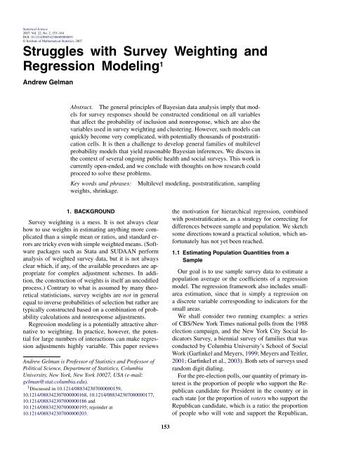
FIG. 1. The proportion of adults surveyed who answered yes in 

the Gallup Poll to the question, “Are you in favor of the death 

penalty for a person convicted of murder?” among those who expressed 

an opinion on the question. Itwouldbeinterestingtoestimate 

these trends in individual states. 

divided by the proportion who will support the Republican; 

it is straightforward to move from estimating a 

population mean to estimating this ratio, as discussed 

in the context of this example by Park, Gelman and 

Bafumi (2004)]. We would also like to use series of 

national polls to estimate state-by-state time trends, for 

example in the support for the death penalty over the 

past few decades. (See Figure 1 for the national trends.) 

For the Social Indicators Survey, we are interested in 

population average responses to questions such as, “Do 

you rate the schools as poor, fair, good or very good?”, 

average responses in subpopulations (e.g., the view of 

the schools among parents of school-age children), and 

so-called “analytical” studies that can be expressed in 

terms of regressions (e.g., predicting total satisfaction 

given demographics and specific attitudes about health 

care, safety, etc.). In this article, we focus on trends 

from 1999 to 2001, as measured by changes in two 

successive Social Indicators Surveys, on a somewhat 

arbitrary selection of questions chosen to illustrate the 

general concerns of the survey. 

Table 1 shows the questions, the estimated average 

responses in each year, and the estimated differences 

and standard errors as obtained using two different 

methods of inference. This paper is centered on the 

puzzle of how these two estimation methods differ. We 

shall get back to this question in a moment after reviewing 

some basic ideas in survey sampling inference. 

1.2 Poststratification and Weighting 

Naive promulgators of Bayesian inference—or the 

modeling approach to inference in general—used to 

say that the method of data collection was irrelevant 

to estimation from survey data. All that matters, from 

this slightly misguided perspective, is the likelihood, or 

the model of how the data came to be. However, as has 

been pointed out by Rubin (1976), the usual Bayesian 

or likelihood analysis implicitly assumes the design 

is “ignorable,” which in a sampling context roughly 

means that the analysis includes all variables that affect 

the probability of a person being included in the 

survey (see Chapter 7 of Gelman et al., 2004, forareview). 

In a regression context, the analysis should include, 

as “X variables,” everything that affects sample selection 

or nonresponse. Or, to be realistic, all variables 

should be included that have an important effect on 

sampling or nonresponse, if they also are potentially 

predictive of the outcome of interest. In a public survey 

such as the CBS polls, a good starting point is the set 

of variables used in their weighting scheme: number 

of adults and number of telephone lines in the sampled 

household; region of the country; and sex, ethnicity, 

age and education level of the respondent (see 

Voss, Gelman and King, 1995). For the Social Indicators 

Survey, we did our own weighting (Becker, 1998) 

TABLE 1 

Weighted 

averages 

Question 1999 2001 

(a) time 

change 

in 

percent 

(b) linear 

regression 

coefficient 

of time 

(a) time 

change 

on logit 

scale 

(b) logistic 

regression 

coefficient 

of time 

Adult in good/excellent health 75% 78% 3.4% (2.4%) 6.6% (1.4%) 0.19 (0.13) 0.48 (0.10) 

Child in good/excellent health 82% 84% 1.7% (1.5%) 1.2% (1.3%) 0.24 (0.21) 0.18 (0.20) 

Neighborhood is safe/very safe 77% 81% 4.5% (2.3%) 4.1% (1.5%) 0.27 (0.14) 0.27 (0.10) 

Estimates for some responses from two consecutive waves of the New York City Social Indicators Survey, and estimated changes, with 

standard errors in parentheses. Changes are estimated in percentages and on the logit scale. In each scale, two estimates are presented: (a) 

simple differences in weighted means and (b) regression controlling for the variables used in the weighting. Approaches (a) and (b) can give 

similar results but sometimes are much different.

SURVEY WEIGHTING AND REGRESSION MODELING 155 

using similar information: number of telephone lines 

(counted as 1/2 for families with intermittent phone 

service), number of adults and children in the family, 

and ethnicity, age and education of the head of household. 

Weights for each survey are constructed by multiplying 

a series of factors. 

In the sampling context, ignorability corresponds 

to the assumption of simple random sampling within 

poststratification cells or, more generally, the assumption 

that, within poststratification cells, the relative 

probabilities of selection are equal. (This is the information 

used in constructing sampling weights.) Adjustment 

for unit nonresponse is implicit in this framework; 

for example, by poststratifying on sex, an analysis 

adjusts simultaneously for differences between men 

and women in probability of inclusion in the sample 

(i.e., probability of being sampled, multiplied by probability 

of responding). We shall ignore item nonresponse 

(or, equivalently, suppose any missing data have 

been randomly imputed; see the discussion in Rubin, 

1996). 

We now review the unified notation for poststratification 

and survey weighting of Little (1991, 1993)and 

Gelman and Carlin (2002); see also Holt and Smith 

(1979). Here we use the notation y,z for variables 

that are observed in the sample only, and X for variables 

that are observed in the sample and known in 

the population. For simplicity, we assume throughout 

this article that the population size is large, so that the 

finite-population quantities of interest (averages, population 

totals or regression coefficients) are essentially 

the same as the corresponding superpopulation quantities. 

Poststratification. The purpose of poststratification 

is to correct for known differences between sample 

and population. In the basic formulation, we have variables 

X whose joint distribution in the population is 

known, and an outcome y whose population distribution 

we are interested in estimating. We shall assume 

X is discrete, and label the possible categories of X 

as poststratification cells j, with population sizes N j 

and sample sizes n j . In this notation, the total population 

size is N = ∑ J 

j=1 N j and the sample size is 

n = ∑ J 

j=1 n j . The implicit model of poststratification 

is that the data are collected by simple random sample 

within each of the J poststrata. The assignment of 

sample sizes to poststrata is irrelevant. In fact, classical 

stratification (in which the sampling really is performed 

within strata) is a special case of poststratification 

as we formulate it. We assume the population 

size N j of each category j is known. These categories 

include all the cross-classifications of the predictors 

X. [In some cases the cell populations are unknown 

and must be estimated. For example, in the Social Indicators 

Survey, we adjust to estimated demographics 

from the Current Population Survey, which includes 

about 2000 New York City residents each year. This is 

enough to give reliable estimates of one-way and twoway 

margins (e.g., the proportion of city residents who 

are white females, white males, black females, black 

males, etc.), but the counts are too sparse to directly estimate 

deep interactions (e.g., the proportion who are 

white females, 30–45, married, with less than a high 

school education, etc.). The usual practical solution in 

this case is to poststratify on the margins (e.g., raking; 

see, e.g., Deville, Sarndal and Sautory, 1993). If 

the whole table of population counts is required, it can 

be estimated using iterative proportional fitting (Deming 

and Stephan, 1940) which sets interactions to be 

as small as possible while being consistent with the 

available population data. For this paper, we shall ignore 

this difficulty and treat the full vector of N j ’s as 

known.] 

The population mean of any survey response can be 

written as a sum over poststrata, 

∑ Jj=1 

N j θ j 

(1) definition of population mean: θ = ∑ Jj=1 

, 

N j 

with corresponding estimate, 

(2) 

poststratified estimate: ˆθ PS = 

∑ Jj=1 

N j ˆθ j 

∑ Jj=1 

N j 

. 

We use the general notation θ j rather than Y j to allow 

for immediate generalization to other estimands such 

as regression coefficients. 

Weighting. When you look at sample survey data 

from a public-use dataset, the “survey weight” looks 

like a unit-level characteristic—just one more column 

in the data—and it is easy to think of it almost 

as a survey response, w i . In this context it seems 

natural to use weighted averages of the form ȳ = 

∑ ni=1 

(w i y i )/ ∑ n 

i=1 w i . 

But survey weights are not attributes of individual 

units—they are constructions based on an entire survey. 

Within any poststratification cell, all units have 

the same poststratification weight adjustment. (In theory, 

continuously-varying survey weights could arise 

from a survey with a continuous range of sampling 

probabilities. For example, one could imagine a survey 

of college-bound students where the probability of

156 A. GELMAN 

TABLE 2 

respid org year survey y state edu age female black adults phones weight 

11352 6140 cbsnyt 7 9158 NA 7 3 1 1 0 2 1 923 

11353 6141 cbsnyt 7 9158 1 39 4 2 1 0 2 1 558 

11354 6142 cbsnyt 7 9158 0 31 2 4 1 0 1 1 448 

11355 6143 cbsnyt 7 9158 0 7 3 1 1 0 2 1 923 

11356 6144 cbsnyt 7 9158 1 33 2 2 1 0 1 1 403 

Data from the first five respondents of a CBS pre-election poll. The weights are listed as just another survey variable, but they are actually 

constructed after the survey has been conducted, so as to match sample with known population information. 

selection is a continuous function of background variables 

[e.g., Pr(selection) = logit −1 (a + b · SAT)]. Or 

one could model nonresponse as a continuous function 

of predictors such as age and previous health status 

in a medical survey. These continuous weights do 

not come up much in the sorts of social surveys under 

consideration in this article, but they are interesting research 

directions that are potentially important in other 

areas of application.) We shall refer to unit weights w i , 

i = 1,...,n, and cell weights W j = n j w i for units i 

within cell j, 

∑ ni=1 

w i y i 

weighted average: ȳ = ∑ ni=1 

w i 

(3) 

= 

∑ Jj=1 

W j ȳ j 

∑ Jj=1 

W j 

. 

Survey weights in general depend on the actual data 

collected as well as on the design of the survey. For example, 

consider the seven CBS polls conducted during 

the week before the 1988 Presidential election. These 

surveys had identical designs and targeted the same 

population. However, the weighting factor assigned to 

men (compared to a factor of 1 for women) varies from 

as low as 1.10 to 1.27 among the seven surveys. The 

different samples happened to contain different ratios 

of men to women and hence needed different adjustments. 

Weighting based on sampling probabilities. Afurther 

complication is that survey weighting is commonly 

performed on some variables using inversesampling 

probabilities rather than poststratification. 

For example, in the Social Indicators Survey we 

assigned weights of 1/2, 1 and 2 for households with 

multiple phone lines, exactly one phone line and intermittent 

phone service, respectively. Unlike poststratification 

weights, these weighting factors are fixed and 

do not depend on the sample. 

These inverse-probability weights are important in 

some survey designs and are sometimes portrayed 

as producing unbiased estimates, but this unbiasedness 

breaks down in the presence of nonresponse. For 

example, some telephone surveys give each respondent 

a weighting factor proportional to the number 

of adults in his or her household; this is an inverseprobability 

weight given that all households are equally 

likely to be selected (after correcting for the number 

of telephone lines) and the respondent is selected 

at random among the adults in the household. 

In practice, however, such weighting overrepresents 

persons in large households, presumably because it 

is easier to find someone at home from a household 

where more adults are living. Poststratification weights 

(which are roughly approximate to weighting by the 

square root of the number of adults in the households) 

give a better fit to the population (Gelman and Little, 

1998). 

In this article we shall assume that any factors associated 

with sampling weights have already been folded 

into the poststratification. For example, consider a survey 

that is poststratified into 16 categories (2 sexes × 

2 ethnicity categories × 4 age ranges), and also has 

telephone weights of 1/2, 1 and 2. The three categories 

of telephone weights would then represent another 

dimension in the adjustment, thus giving a total 

of 48 categories. We recognize that treating this 

weighting as pure poststratification is an oversimplification; 

for one thing, sampling variances for poststratified 

estimates are generally different from those for 

fixed weights (see, e.g., Binder, 1983; LuandGelman, 

2003). 

1.3 Competing Methods of Estimation: Weighted 

Averages, Weighted Regression and 

Unweighted Regression Controlling for X 

Many researchers have noted the challenge of using 

survey weights in regression models (as reviewed, e.g.,


TABLE 3 

True 

Different standard error estimates 

standard assuming conditioning assuming design- 

Opinion of NYC error SRS on weights inv-prob based 

Became a better place 2.2% 1.2% 2.5% 1.9% 2.1% 

Remained the same 2.0% 1.2% 2.3% 1.6% 1.9% 

Gotten worse 2.0% 1.2% 2.4% 1.7% 2.0% 

From a simulation study: true standard error and four different standard error estimates for a question on the 

Social Indicators Survey. Ignoring the weighting or treating the weights as constant underestimates uncertainty, 

whereas uncertainty is overestimated by treating the weights as inverse probabilities. Accurate standard errors 

can be obtained using a jackknife-like procedure that explicitly takes account of the design of the weighting 

procedure. From Lu and Gelman (2003). 

by DuMouchel and Duncan, 1983; Kish,1992; Pfeffermann, 

1993). For the goal of estimating a population 

mean, it is standard to use the weighted average (3), but 

it is not so clear what to do in more complicated analyses. 

For example, when estimating a regression of y on 

z, one recommended approach is to use weighted least 

squares, and another option is to perform unweighted 

regression of y on z, also controlling for the variables 

X that are used in the weighting. 

Computing standard errors is not trivial for weighted 

estimates, whether means or regressions, because the 

weights themselves generally are random variables that 

depend on the data (Yung and Rao, 1996). In particular, 

correct classical standard errors cannot simply be 

obtained from the data and the weights; one also needs 

to know the procedure used to create the weights. Table 

3 illustrates problems with some variance estimates 

that do not account for the weighting design. Similarly, 

with regressions, simple weighted regression procedures 

do not in general give correct standard errors. 

1.4 The Crucial Role of Interactions 

Consider a regression of y on z, estimated in some 

way from a survey where inclusion probabilities depend 

on X. In general, y can depend on both X and 

z, in which case the appropriate way to estimate the 

regression of y on z is to regress y on X, z andthenaverage 

over the population distribution of X. In general, 

estimating the regression of y on z requires estimation 

of the relation between z and X as well (Graubard and 

Korn, 2002). Because of the potential dependence of z 

and X, it can be important to include interactions between 

these predictors in the model for y, evenifthe 

ultimate goal is simply to estimate the relation between 

y and z. 

In our survey adjustment framework, once a model 

includes interactions, poststratification is necessary in 

order to estimate population regression coefficients. 

For a simple example, suppose we are interested in 

the population regression of log earnings on height (in 

inches), using a survey that is adjusted to match the 

proportion of men and women in the population. The 

estimated regression (see Gelman and Hill, 2007) including 

the interaction is 

y = log(earnings) 

= 8.4 + 0.017 · height − 0.079 · male 

+ 0.007 · height · male + error. 

For any given height z, the expected value of log earnings 

is 

(4) 

E(y|z) = 8.4 + 0.017z 

− 0.079 · E(male|height = z) 

+ 0.007z · E(male|height = z). 

Here, E(male|height = z) would be estimated from 

the survey itself; most likely we would do this by fitting 

a linear regression (with Gaussian errors) of height 

given sex, and then simply using Bayes’ rule, along 

with the population proportions of men and women, 

to compute the conditional probability. 

The conditional expectation (4) is not, in general, 

a linear function of z. Thus, although we can define 

the population regression of log earnings on height—it 

is the result of fitting a simple linear regression of y on 

z to the entire population—it is not clear why it should 

be of any interest. 

This difficulty in interpreting regression coefficients 

in the context of survey adjustments is one reason we 

have been careful in Section 1.1 to consider estimands 

that are simple comparisons of population averages. 

We illustrate with the goal of estimating the average

158 A. GELMAN 

difference in log earnings between whites and nonwhites; 

this is also a regression, but because the predictor 

z is binary, it is defined unambiguously as a difference. 

Again, we suppose for simplicity that the survey 

is adjusted only for sex. The estimated regression fit, 

including the interaction, is 

y = log(earnings) 

= 9.5 − 0.02 · white + 0.20 · male 

+ 0.41 · white · male + error. 

The population difference in log earnings is then 

E(y|white = 1) − E(y|white = 0) 

=−0.02 + 0.20 · (E(male|white = 1) 

− E(male|white = 0) ) 

+ 0.41 · E(male|white = 1), 

and the factors E(male|white = 0) and E(male| 

white = 1) can be estimated from the data. More generally, 

this example illustrates that, once we fit an interaction 

model in a survey adjustment context, we cannot 

simply consider a single regression coefficient (in this 

case, for white) but rather must also use the interacted 

terms in averaging over poststratification cells. 

Our focus in this article is on the relation between 

the model for the survey response and the corresponding 

weighted-average estimate. The ultimate goal is to 

have a model-based procedure for constructing survey 

weights, or conversely to set up a framework for regression 

modeling that gives efficient and approximately 

unbiased estimates in a survey-adjustment context. 

2. THE CHALLENGE 

2.1 Estimating Simple Averages and Trends 

We now return to the example of Table 1. The goal is 

to estimate Y 2001 − Y 1999 , the change in population average 

response between two waves of the Social Indicators 

Survey. This can be formulated as the coefficient 

β 1 in a regression of y on time: y = β 0 + β 1 z + error, 

where the data from the two surveys are combined, and 

z = 0 and 1 for respondents of the 1999 and 2001 surveys, 

respectively. 

A more general model is y = β 0 +β 1 z+β 2 X+error, 

where β 2 is a vector of coefficients for the variables X 

used in the weighting. Now the quantity of interest is 

β 1 + β 2 (X 2001 − X 1999 ), to account for demographic 

changes between the two years. For New York City 

between 1999 and 2001, these demographic changes 

were minor, and so it is reasonable to simply consider 

β 1 to be the quantity of interest. 

This brings us to the puzzle of Table 1. For each 

of three binary outcomes y, we compute the weighted 

mean for each year, ȳw 1999 and ȳw 

2001 , and two estimates 

of the change: 

• Our first estimate is the simple 

√ 

difference, ȳw 

2001 − 

ȳw 

1999, 

with standard error var(ȳw 

2001) 

+ var(ȳ1999 w ), 

where the sampling variances are computed using 

the design of the weights (as in the rightmost column 

in Table 3). 

• Our other estimate is obtained by linear regression. 

We combine the data from the two surveys into a 

single vector, y = (y 1999 ,y 2001 ), and create an associated 

indicator vector z that equals 0 for the data 

from 1999 and 1 for the data from 2001. We fit a 

linear regression of y on z, also controlling for the 

variables X used in the weighting. (These X variables 

are number of adults in the household, number 

of children in the family, number of telephone lines, 

marital status, and sex, age, ethnicity and education, 

and ethnicity × education for the head of household.) 

To estimate the change from 1999 to 2001, 

we use the coefficient of z, with standard error automatically 

coming from the (unweighted) regression. 

As indicated in the third and fourth columns of Table 

1, the regression coefficient and the change in 

weighted averages tend to have the same sign, but the 

two estimates sometimes differ quite a bit in magnitude. 

(Similar results are obtained if we work on the 

logit scale, as can be seen from the final two columns 

of the table.) 

What should we believe? For this particular example, 

the direct analysis of weighted averages seems 

more believable to us, since we specifically created 

the weighting procedure for the goal of estimating 

these citywide averages. More generally, however, using 

weighted averages is awkward and we would prefer 

to use the more general techniques of regression and 

poststratification. 

Where do we go from here? We would like an approach 

to statistical analysis of survey data that gives 

the right answers for simple averages and comparisons, 

and can be smoothly generalized to more complicated 

estimands. 

2.2 Deep Poststratification 

One of the difficulties of survey weighting is that 

the number of poststratification cells can quickly become 

large, even exceeding the number of respondents.


This leads naturally to multilevel modeling to obtain 

stable estimates in all the poststratification cells, even 

those with zero or one respondent. Choices must then 

be made in the modeling of interactions. 

For example, in our time-trend estimation problem, 

we could model y = β 0 + β 1 z + β 2 X + β 3 Xz + error, 

where β 3 is a vector of coefficients for the interaction 

of X and time. We would then be interested in 

β 1 + β 2 (X 2001 − X 1999 ) + β 3 X 2001 (as in the example 

at the end of Section 1.4). Where should the interaction 

modeling stop? A simulation study (Cook and 

Gelman, 2006) suggests that, in this example, efficient 

and approximately unbiased estimators are obtained by 

including interactions of the time indicator with all the 

survey adjustment factors; as a general approach, however, 

including all interactions can yield unstable estimates. 

The practical problem of adjusting for survey 

nonresponse leads to general questions of inference under 

multiway interactions, an issue that becomes even 

more relevant in small-area estimation. 

Gelman and Carlin (2002) and Park, Gelman and Bafumi 

(2004) discuss the estimation of state-level opinions 

from national polls, using a hierarchical logistic 

regression with demographics and state effects, followed 

by poststratification on Census population totals 

for 64 demographic categories in each of the 50 states. 

The method worked well, but it is not clear how it 

would perform if the model included interactions of 

demographic and state effects. 

3. USING REGRESSION MODELING TO CONNECT 

WEIGHTING AND POSTSTRATIFICATION 

When cell means are estimated using certain linear 

regression models, poststratified estimates can be interpreted 

as weighted averages (Little, 1991, 1993). The 

idea is to work with the poststratified estimate (2)— 

an average over cell estimates ˆθ j , with the regression 

model providing the ˆθ j ’s based on characteristics of the 

cells j. Under certain conditions, the poststratified estimate 

can be reinterpreted as a weighted average of the 

form (3), and then we can solve for the cell weights W j 

and the unit weights w i . 

3.1 Classical Models 

Full poststratification. The simplest case is full 

poststratification of raw data, in which case the cell 

estimates are the cell means, ˆθ j =ȳ j ,and(2) becomes 

∑ Jj=1 

full poststratification: ˆθ PS N j ȳ j 

= ∑ Jj=1 

, 

N j 

which is equivalent to (3) with cell weights W j ∝ N j or 

unit weights w i ∝ N j(i) /n j(i) ,wherej(i) is the poststratification 

cell to which unit i belongs. 

This estimate can also be viewed as a classical regression 

including indicators for all J poststratification 

cells. 

No weighting. The other extreme is no weighting, 

that is, unit weights w i = 1foralli, which is equivalent 

to poststratification if the cell estimates ˆθ j are all equal 

to the sample mean ȳ, which in turn corresponds to 

classical regression including only a constant term. 

Classical regression on cell characteristics. Intermediate 

cases of weighting can be obtained by regression 

models that include information about the poststratification 

cells without going to the extreme of fitting 

a least-squares predictor to each cell. For example, 

in the CBS/New York Times pre-election surveys, 

one could regress y on indicators for sex, ethnicity, age, 

education and region, without necessarily including all 

their interactions. 

Suppose the regression model is y ∼ N(Xβ, σ 2 y I). 

We shall use X to represent the n × k matrix of predictors 

in the data, and X pop to represent the J × k 

matrix of predictors for the J poststratification cells. 

We also label the vector of poststratum populations as 

N pop = (N 1 ,...,N J ), with a sum of N = ∑ J 

j=1 N j . 

The estimated vector of regression coefficients is 

then ˆβ = (X t X) −1 X t y, and the estimated cell means 

are X pop ˆβ. The poststratified estimate of the population 

mean is then 

(5) 

(6) 

classical regression: 

ˆθ PS = 1 N 

J∑ 

j=1 

N j (X pop 

j 

ˆβ) 

= 1 N (N pop ) t X pop (X t X) −1 X t y, 

which can be written as ˆθ PS = 1 n 

∑ ni=1 

w i y i , with a 

vector of unit weights, 

(7) 

w = 

( n 

N (N pop ) t X pop (X t X) −1 X t ) t 

. 

For convenience, we have renormalized these weights 

to sum to n (see below). In (7), w is a vector of length 

n that takes on at most J distinct values. The vector of 

J possible unit weights (corresponding to units in each 

of the J poststrata) is 

(8) 

w pop = 

( n 

N (N pop ) t X pop (X t X) −1 (X pop ) t ) t 

,

160 A. GELMAN 

FIG. 2. Equivalent unit weights w i for one of the CBS/New York Times surveys, based on a series of models fit first using classical 

regression and then using Bayesian hierarchical regression. The models are nested, controlling for (1) male/female, (2)also black/white, 

(3) also male/female × black/white, (4)also four age categories, (5)also four education categories, (6)also age × education and (7) 

also state indicators. Each model includes more factors and thus has more possible weights, which are renormalized to average to 1 for 

each model. For the Bayes models, the indicators for age, education, age × education and state are given independent batches of varying 

coefficients. For the classical weights, model (7) is not included because of collinearity. 

The lines in each graph connect the weights for individual respondents, which are divided into successively more categories as predictors 

are added to the models. 

and the poststratified estimate can also be expressed as 

ˆθ PS = 1 n 

J∑ 

j=1 

w pop 

j 

ȳ j . 

The key result that makes the above computations 

possible—that allows ˆθ PS to be interpreted as 

a weighted average of data—is that the derived unit 

weights w in (7) sumton. The identity ∑ n 

j=1 w j = n 

can be proved using matrix algebra but is more easily 

derived from an invariance in the classical regression 

model. With a least-squares regression, if a constant is 

added to all the data, that same constant will be added 

to the intercept, with the other coefficients not changing 

at all. Adding a constant to the intercept adds that 

same constant to ˆθ PS in (5). We have thus established 

that adding a constant to each data point y i adds that 

same constant to ˆθ PS ; thus, when ˆθ PS is expressed as 

ˆθ PS = 1 n 

∑ ni=1 

w i y i ,thesew i /n’s must sum to 1. 

The left panel of Figure 2 shows the unit weights 

obtained by fitting a sequence of classical regression 

models to the CBS/New York Times survey data. As 

more factors and interactions are included, the weights 

become more variable. 

3.2 Hierarchical Models 

We next consider the estimates that arise when applying 

the basic poststratification formula (2) when the 

cell means ˆθ j are estimated using hierarchical models. 

As we shall see, we can formulate the resulting ˆθ PS as a 

weighted average as in (3). In the classical estimates we 

have just considered, the equivalent weights w i depend 

on the structure of the model and the values of the predictors 

X [see, e.g., (8)]. In contrast, with hierarchical 

models, we find that the w i ’s depend on the response 

variable y being analyzed; for example, the vector of 

weights for the question on the respondent’s health will 

be different than the vector of weights for the respondent’s 

perception of the public schools. In our analysis 

we shall suppose that a particular response variable y 

of interest has been selected (e.g., vote preference in 

the pre-election polls). 

Hierarchical regression. The results in the previous 

section can be immediately generalized to multilevel 

regression models in which some of the coefficients are 

batches of indicator variables. We shall generalize the 

regression model to y ∼ N(Xβ, y ) with a prior distribution 

on β of the form β ∼ N(0, β ). For simplicity, 

we assume independence of the components of β in 

the prior distribution, conditional on hyperparameters 

for the variance components. [In practice, the covariance 

matrix β would come from a fitted hierarchical 

model, and our analysis ignores uncertainty in the 

estimated hyperparameters. A fully Bayesian analysis


would continue by averaging over the posterior distribution 

of β , which in turn would lead to a posterior distribution 

of equivalent weights; which might be summarized 

by a posterior mean, thus leading to posterior, 

or consensus, weights. Rao (2003) discusses this issue 

from a classical sampling-theory perspective.] 

The prior precision matrix β 

−1 is then diagonal, 

with zeroes for nonhierarchical regression coefficients 

(including the constant term in the regression). For example, 

consider a regression for the CBS/New York 

Times polls, with the following predictors: 

• A constant term 

• An indicator for sex (1 if female, 0 if male) 

• An indicator for ethnicity (1 if black, 0 otherwise) 

• Sex × ethnicity 

• 4 indicators for age categories 

• 4 indicators for education categories 

• 16 age × education indicators. 

The classical regression has 1 + 1 + 1 + 1 + 3 + 3 + 

9 = 19 predictors (avoiding collinearity by excluding 

the baseline age and education categories). The hierarchical 

regression has 1 + 1 + 1 + 1 + 4 + 4 + 16 = 28 

predictors, and its prior precision matrix has the form 

−1 

β 

= Diag(0, 0, 0, 0,σ −2 

age ,σ−2 age ,σ−2 age ,σ−2 age ,σ−2 edu , 

σedu −2 ,σ−2 edu ,σ−2 edu ,σ−2 age.edu ,...,σ−2 age.edu ), 

with the parameters σ age , σ edu and σ age.edu estimated 

from data. 

The estimated vector of regression coefficients is 

then ˆβ = (X t y 

−1X 

+ −1 β )−1 X t y 

−1 y and expressions 

(6)–(8) become 

(9) 

Bayes poststratification: 

ˆθ PS = 1 N (N pop ) t X pop 

× (X t y 

−1 X + −1 β )−1 X t y −1 y, 

( n 

w = 

N (N pop ) t X pop 

× (X t −1 

y 

X + −1 

( n 

w pop = 

N (N pop ) t X pop 

× (X t −1 

y 

β 

) t )−1 X t y 

−1 , 

) t X + −1 β )−1 (X pop ) t y 

−1 . 

Conditional on the variance parameters in y and 

beta , then estimates from this model correspond to 

weighted averages. 

The right panel of Figure 2 shows the unit weights 

obtained by fitting a sequence of Bayesian models to 

the CBS/New York Times poll. The first three models 

are actually identical to the classical (nonhierarchical) 

versions, since we assign noninformative uniform 

prior distributions to the coefficients for sex, ethnicity 

and their interactions. Models 4 and 5 are similar to 

the classical fits because age and education have only 

four categories, so there is little information available 

for partial pooling of these effects (see Gelman, 2006). 

The weights in model 6, with age × education interactions 

included, are smoothed somewhat compared to 

the corresponding classical model. Finally, introducing 

state effects leads to a downweighting of some of respondents 

in states that happen to be overrepresented in 

the survey, and an upweighting for respondents in the 

undersampled states. There is no corresponding classical 

model here because the survey does not actually 

include data from all 50 states. 

Exchangeable normal model. To understand these 

formulas better, we consider the special case of an exchangeable 

normal model for the J cell means (see 

also Lazzeroni and Little, 1998; Elliott and Little, 

2000). This model can be expressed in terms of the cell 

means, 

ȳ j ∼ N(θ j ,σ 2 /n j ), 

θ j ∼ N(µ, σ 2 θ ). 

This is a special case of the hierarchical regression 

model discussed above, so we already know that the 

poststratified estimate, conditional on the (estimated) 

variance parameters σ y ,σ θ , can be expressed as a 

weighted average of the cell means, ȳ j , or equivalently 

as a weighted average of the data points y i . 

In this simple example, however, we can gain some 

understanding by deriving algebraic expressions for the 

weights. Our goal is to express them in terms of the 

completely smoothed weights, w j = 1, and the weights 

from full poststratification, w j = N j /N 

n j /n . 

We start with the posterior means (conditional on the 

variance parameters) of the cell means. We write these 

as ˆθ k ,k= 1,...,J (using k as a subscript rather than j 

because this results in more convenient notation later), 

(10) 

where 

(11) 

ˆθ k = (n k/σy 2)ȳ k + (1/σθ 2) ˆµ 

n k /σy 2 + 1/σ θ 

2 , 

ˆµ = 

∑ Jk=1 ȳ k /(σ 2 y /n k + σ 2 θ ) 

∑ Jk=1 

1/(σ 2 y /n k + σ 2 θ ) .

162 A. GELMAN 

We can combine (10) and(11) to express each ˆθ j as a 

linear combination of the cell means ȳ k , 

J∑ 

ˆθ k = c kj ȳ j . 

j=1 

After some algebra, we can write these coefficients as 

⎧ 

σy 

2 ⎪⎨ A k A j /A, for j ≠ k, 

c kj = 

n k 

⎪⎩ σθ 2A k + σ y 

2 A 2 k 

, for j = k, 

n k 

where 

A k = 

J∑ 1 

σy 2/n k + σθ 

2 . 

k=1 

The payoff now comes in computing the poststratified 

estimate, 

J∑ 

ˆθ PS = N k ˆθ/N 

k=1 

= 

J∑ 

J∑ 

k=1 j=1 

N k 

N c kj y¯ 

j , 

equating this to ∑ j 

j=1 W j y¯ 

j and thus deriving the cell 

weights, 

W j = 

J∑ 

k=1 

N k 

N c kj 

= A j 

[ 

Nj 

N σ 2 θ + J ∑ 

k=1 

N k 

N 

A k 

A 

σy 

2 ] 

. 

n k 

The implicit unit weights are then w pop 

j 

= (n/n j )W j , 

or 

(12) 

w pop 

j 

[ 

n Nj 

= A j 

n j N σ θ 2 + σ y 

2 

AN 

n 

= 

σ 2 y + n j σ 2 θ 

× 

[ 

Nj 

N σ θ 2 + σ y 

2 

N 

J∑ 

k=1 

] 

N k 

A k 

n k 

∑ Jk=1 

N k /(σ 2 y + n kσ 2 θ ) 

∑ Jk=1 

n k /(σ 2 y + n kσ 2 θ ) ]. 

The ratio of sums in (12) is a constant (given the fitted 

model) that does not depend on j. Let us approximate 

it by N/n (which is appropriate if the sample 

proportions n k /N k are independent of the group sizes 

N k ). Under this approximation, the unit weights can be 

written as 

approximate w pop 

j 

(13) 

n j /σy 

2 = 

n j /σy 2 + 1/σ θ 

2 

· Nj /N 

n j /n 

1/σθ 

2 + 

n j /σy 2 + 1/σ θ 

2 · 1, 

which is a weighted average of the full poststratification 

unit weight, N k/N 

n k /n 

, and the completely smoothed 

weight of 1. Hierarchical poststratification is thus approximately 

equivalent to a shrinkage of weights by 

the same factors as in the shrinkage of the parameter 

estimates (10). 

Thus, as with hierarchical regression models in general, 

the amount of shrinkage of the weights depends 

on the between- and within-stratum variance in the outcome 

of interest, y. 

Other hierarchical models. Lazzeroni and Little 

(1998) and Elliott and Little (2000) discuss various 

hierarchical linear regression models, including combinations 

of the two models described above (i.e., a 

hierarchical regression with a cell-level variance component) 

and models with correlations between adjacent 

cell categories for ordered predictors. 

Another natural generalization is to use logistic regression 

for binary inputs. Unfortunately, when we 

move away from linear regression, we abandon the 

translation invariance of the parameter estimates (i.e., 

the property that adding a constant to all the data affects 

only the constant term and none of the other regression 

coefficients). As a result, for logistic regression, 

the poststratified estimate ˆθ PS is no longer a weighted 

average of the data, even after controlling for the variance 

parameters in the model. However, we suspect 

that the model could be linearized, yielding approximate 

weights. 

3.3 Properties of the Model-Based Poststratified 

Estimates 

Standard errors. The variance of the poststratified 

estimate, ignoring sampling variation in X, can be expressed 

using various formulas, 

var( ˆθ PS ) = 1 n∑ 

n 2 wi 2 σ y 2 = 1 J∑ 

(w pop 

j 

) 2 n j σy 

2 n 

= 1 

nN 

i=1 

J∑ 

j=1 

j=1 

w pop 

j 

N pop 

j 

σy 2 .


Any of these equivalent expressions can be viewed as 

the posterior variance of θ given a noninformative prior 

distribution on the regression coefficients, and ignoring 

posterior uncertainty in σ y (Little, 1993). 

Dependence of implicit weights on the outcome variable. 

Classical survey weights depend only on the n j ’s 

and the N j ’s, as well as the design matrix X (used, e.g., 

to define the margins used in raking), but do not formally 

depend on y. (There is an informal dependence 

on y in the sense that there is no urgency to weight 

on variables X that do not help predict outcomes y of 

interest.) Similarly, the implicit weights (7) obtained 

from a classical regression model depend only on n, N 

and X, not on y. 

However, the implicit weights (9) from hierarchical 

regression do depend on the data, implicitly, through 

the hyperparameters in y and β , which are estimated 

from the data. Thus, the appropriate weights 

could differ for different survey responses. 

4. WHERE TO GO NEXT 

There are currently two standard approaches to adjusting 

for known differences between sample and population 

in survey data: weighting and regression modeling. 

Practical limitations of weighting. The weighting 

approach has the advantage of giving simple estimates 

for population averages but has several disadvantages. 

First, it is not generally clear how to apply weights to 

more complicated estimands such as regression coefficients. 

There has been some work on weighted regression 

for surveys (e.g., DuMouchel and Duncan, 

1983; Pfeffermann, 1993) but these procedures are not 

very flexible, which is one reason why the modeling 

approach is more popular for problems such as 

small-area estimation (Fay and Herriot, 1979). A second 

problem with weighted estimates is that standard 

errors are more difficult to evaluate (recall Table 3). 

Finally, weighting may be “dirty” but it is not always 

“quick”: actually constructing the weighting for a survey 

is more difficult than you might think. Creating 

practical weights requires arbitrary choices about inclusion 

of weighting factors and interactions, pooling 

of weighting cells and truncation of weights. (For example, 

in the Social Indicators Survey, we decided 

to weight on some interactions and not others in order 

to control variability of the weights. While setting 

up the weighting procedure, we repeatedly compared 

weighted estimates to Census values for various outcomes 

that we thought could be “canaries in the coal 

mine” if the survey estimate did not fit the population. 

These “canary” variables included percentage of 

New York City residents who are U.S. citizens, the percent 

who own their own home and income quintiles.) 

The resulting vector of weights is in general a complicated 

and not-fully-specified function of data and prior 

knowledge. Subjective choices arise in virtually all statistical 

methods, of course, but good advice on creating 

weights tends to be much vaguer than for other methods 

in the statistical literature (see, e.g., Lohr, 1999). 

Practical limitations of modeling. Regression modeling 

is easy to do—even hierarchical regression is becoming 

increasingly easy in Bugs, Stata and other software 

packages (see, e.g., Centre for Multilevel Modelling, 

2005; Gelman and Hill, 2007)—but for analysis 

of survey data it has the disadvantage that, to combine 

with population information, the regression must theoretically 

condition on all the poststratification cells, 

which can lead to very complicated models—more 

complicated than we are comfortable with in current 

statistical practice—even in surveys of moderate size 

(see Section 2.2). When a model is too complicated, it 

becomes difficult to interpret or use the results, leading 

to awkward situations such as in Table 1,wherewe 

simply cannot trust the regression coefficients for time 

trends in the Social Indicators Survey. 

It is a delicate point, because sometimes we do have 

confidence in regression coefficients, even with complicated 

hierarchical models with many parameters. 

For example, as discussed in Gelman and Carlin (2002) 

and Park, Gelman and Bafumi (2004), hierarchical regression 

combined with poststratification performs excellently 

at estimating state-level opinions from the national 

CBS/New York Times polls. So it is not just the 

number of parameters that is important, but rather some 

connection between the model and the quantities of interest, 

which is somehow more difficult to establish in 

the models whose results are shown in Table 1. 

Putting it together using hierarchical models and 

poststratification. Our ideal procedure should be as 

easy to use as hierarchical modeling, with population 

information included using poststratification as in (1). 

The procedure should feature a smooth transition from 

classical weighting so that when different estimation 

methods give different results, it is possible to understand 

this difference as a result of interactions in the 

model (as discussed by Graubard and Korn, 2002). 

How do we get there? One place to start is to focus 

on examples such as in Table 1 where different methods 

give different answers, and try to figure out which,

164 A. GELMAN 

if either, of the two estimates makes sense. A parallel 

approach is through simulation studies—for greater realism, 

these can often be constructed using subsamples 

of actual surveys—as well as theoretical studies of the 

bias and variance of poststratified estimates with moderate 

sample sizes. In addition, a full hierarchical modeling 

approach should be able to handle cluster sampling 

(which we have not considered in this article) 

simply as another grouping factor. 

We would like a general modeling procedure that 

gives believable estimates for time trends and as a 

byproduct produces a good set of weights that can be 

used for simple estimands. Given the difficulties with 

current methods for weighting and modeling, we believe 

this approach is of both practical and theoretical 

interest. 

ACKNOWLEDGEMENTS 

We thank Samantha Cook, John Carlin, Julian Teitler, 

Sandra Garcia, Danny Pfeffermann and several reviewers 

for helpful discussions and comments, and the National 

Science Foundation for financial support. 

REFERENCES 

BECKER, D. E. (1998). The New York City Social Indicators Survey: 

An analysis of the weighting procedure. Technical report, 

School of Social Work, Columbia Univ. 

BINDER, D. A. (1983). On the variances of asymptotically normal 

estimators from complex surveys. Internat. Statist. Rev. 51 279– 

292. MR0731144 

CENTRE FOR MULTILEVEL MODELLING (2005). Software 

reviews of multilevel analysis packages. Available 

at www.cmm.bristol.ac.uk/learning-training/multilevel-msoftware/index.shtml. 

COOK, S.R.andGELMAN, A. (2006). Survey weighting and regression. 

Technical report, Dept. Statistics, Columbia Univ. 

DEMING, W.E.andSTEPHAN, F. F. (1940). On a least squares 

adjustment of a sampled frequency table when the expected 

marginal totals are known. Ann. Math. Statist. 11 427–444. 

MR0003527 

DEVILLE, J.,SARNDAL, C.andSAUTORY, O. (1993). Generalizing 

raking procedures in survey sampling. J. Amer. Statist. Assoc. 

88 1013–1020. 

DUMOUCHEL, W.H.andDUNCAN, G. J. (1983). Using sample 

survey weights in multiple regression analyses of stratified samples. 

J. Amer. Statist. Assoc. 78 535–543. 

ELLIOTT, M.R.andLITTLE, R. J. A. (2000). Model-based alternatives 

to trimming survey weights. J. Official Statistics 16 

191–209. 

FAY, R.E.andHERRIOT, R. A. (1979). Estimates of income for 

small places: An application of James–Stein procedures to census 

data. J. Amer. Statist. Assoc. 74 269–277. MR0548019 

GARFINKEL, I.,KAUSHAL, N.,TEITLER, J.andGARCIA, S. 

(2003). Vulnerability and resilience: New Yorkers respond to 

9/11. Technical report, School of Social Work, Columbia Univ. 

GARFINKEL, I.andMEYERS, M. K. (1999). New York City social 

indicators 1997: A tale of many cities. Technical report, School 

of Social Work, Columbia Univ. 

GELMAN, A. (2006). Prior distributions for variance parameters in 

hierarchical models. Bayesian Anal. 1 515–533. MR2221284 

GELMAN, A.andCARLIN, J. B. (2002). Poststratification and 

weighting adjustments. In Survey Nonresponse (R.M.Groves, 

D. A. Dillman, J. L. Eltinge and R. J. A. Little, eds.) 289–302. 

Wiley, New York. 

GELMAN, A.,CARLIN, J.B.,STERN, H.S.andRUBIN, D.B. 

(2004). Bayesian Data Analysis, 2nd ed. CRC Press, London. 

MR2027492 

GELMAN,A.andHILL, J. (2007). Data Analysis Using Regression 

and Multilevel/Hierarchical Models. Cambridge Univ. Press. 

GELMAN, A.andLITTLE, T. C. (1998). Improving on probability 

weighting for household size. Public Opinion Quarterly 62 

398–404. 

GRAUBARD, B.I.andKORN, E. L. (2002). Inference for superpopulation 

parameters using sample surveys. Statist. Sci. 17 73– 

96. MR1910075 

HOLT, D.andSMITH, T. M. F. (1979). Post stratification. J. Roy. 

Statist. Soc. Ser. A 142 33–46. 

KISH, L. (1992). Weighting for unequal P i . J. Official Statistics 8 

183–200. 

LAZZERONI, L.C.andLITTLE, R. J. A. (1998). Random-effects 

models for smoothing poststratification weights. J. Official Statistics 

14 61–78. 

LITTLE, R. J. A. (1991). Inference with survey weights. J. Official 

Statistics 7 405–424. 

LITTLE, R. J. A. (1993). Post-stratification: A modeler’s perspective. 

J. Amer. Statist. Assoc. 88 1001–1012. 

LOHR, S. (1999). Sampling: Design and Analysis. Duxbury, Pacific 

Grove, CA. 

LU, H.andGELMAN, A. (2003). A method for estimating designbased 

sampling variances for surveys with weighting, poststratification 

and raking. J. Official Statistics 19 133–151. 

MEYERS, M.K.andTEITLER, J. O. (2001). New York City social 

indicators 1999: Pulling ahead, falling behind. Technical report, 

School of Social Work, Columbia Univ. 

PARK, D.K.,GELMAN, A.andBAFUMI, J. (2004). Bayesian 

multilevel estimation with poststratification: State-level estimates 

from national polls. Political Analysis 12 375–385. 

PFEFFERMANN, D. (1993). The role of sampling weights when 

modeling survey data. Internat. Statist. Rev. 61 317–337. 

RAO, J. N. K. (2003). Small Area Estimation. Wiley, Hoboken, NJ. 

MR1953089 

RUBIN, D. B. (1976). Inference and missing data (with discussion). 

Biometrika 63 581–592. MR0455196 

RUBIN, D. B. (1996). Multiple imputation after 18+ years (with 

discussion). J. Amer. Statist. Assoc. 91 473–520. 

VOSS, D.S.,GELMAN, A.andKING, G. (1995). Preelection 

survey methodology: Details from eight polling organizations, 

1988 and 1992. Public Opinion Quarterly 59 98–132. 

YUNG, W.andRAO, J. N. K. (1996). Jackknife linearization variance 

estimators under stratified multi-stage sampling. Survey 

Methodology 22 23–31.

Struggles with Survey Weighting and Regression Modeling paper

You also want an ePaper? Increase the reach of your titles

Delete template?

Save as template?