solutions to homework exercises

Chapter 1 Solutions to Homework;
SPRING 2012
1. (a) The sample space is
{1,2,3,4,5,6,7,8,9, 10}.
(b) A = {1,3,5,7,9}.
(c) B = {8,10}
(d) The outcome is larger than 6.
2. P(A) = 5/10 = 0.5000. P(B) = 2/10 =
0.2000. P(C) = 4/10 = 0.4000.
3. (a) P(1) = 0.30,P(2) = 0.15,P(3) =
0.25,P(4) = 0.20,P(5) = 0.10. This
is mathematically valid; all numbers are
nonnegative and they sum to one.
(b) P(1) = 0.30,P(2) = 0.15,P(3) =
0.20,P(4) = 0.20,P(5) = 0.10. Not
valid; these numbers sum to 0.95, not 1.
(c) P(1) = 0.30,P(2) = 0.15,P(3) =
0.25,P(4) = 0.20,P(5) = 0.20. Not
valid; these numbers sum to 1.10, not 1.
(d) P(1) = 0.30,P(2) = 0.15,P(3) =
0.25,P(4) = 0.40,P(5) = −0.10. Not
valid; while these numbers sum to one,
negative probabilities are not allowed.
4. (a) P(A) = 0.30 + 0.25 + 0.10 = 0.65.
(b) P(B) = 0.15 + 0.20 = 0.35.
(c) P(C) = 0.20.
(d) P(D) = 0.25 + 0.20 + 0.10 = 0.55.
(e) P(E) = 0.30 + 0.25 = 0.55.
5. (a) P(A or B) = P(A)+P(B) = 0.30+
0.55 = 0.85.
(b) P(A c ) = 1 − P(A) = 1 − 0.30 =
0.70.
(c) P(B c ) = 1 − P(B) = 1 − 0.55 =
0.45.
6. By Rule 6, P(A or B) = P(A) + P(B) −
P(AB) = 0.65 + 0.45 − 0.30 = 0.80.
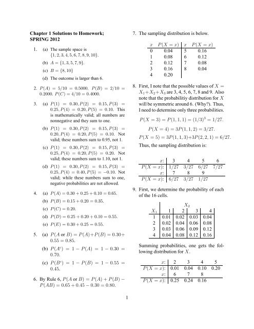
7. The sampling distribution is below.
x P(X = x) x P(X = x)
0 0.04 5 0.16
1 0.08 6 0.12
2 0.12 7 0.08
3 0.16 8 0.04
4 0.20
8. First, I note that the possible values of X =
X 1 +X 2 +X 3 are 3, 4, 5, 6, 7, 8 and 9. Also
note that the probabilitiy distribution for X
will be symmetric around 6. (Why?). Thus,
I need to determine only three probabilities.
P(X = 3) = P(1, 1, 1) = (1/3) 3 = 1/27.
P(X = 4) = 3P(1, 1, 2) = 3/27.
P(X = 5) = 3P(1, 1, 3)+3P(2, 2, 1) = 6/27.
Thus, the sampling distribution is:
x: 3 4 5 6
P(X = x): 1/27 3/27 6/27 7/27
x: 7 8 9
P(X = x): 6/27 3/27 1/27
9. First, we determine the probability of each
of the 16 cells.
X 2
X 1 1 2 3 4
1 0.01 0.02 0.03 0.04
2 0.02 0.04 0.06 0.08
3 0.03 0.06 0.09 0.12
4 0.04 0.08 0.12 0.16
Summing probabilities, one gets the following
distribution for X.
x: 2 3 4 5
P(X = x): 0.01 0.04 0.10 0.20
x: 6 7 8
P(X = x): 0.25 0.24 0.16
1

Chapter 1 Solutions to Homework Continued
10. The possible values of X are: 3, 4, . . . , 12.
Probabilities are given below.
P(X = 3) = P(1,1,1) = (0.1) 3 = 0.001.
P(X = 4) = 3P(1,1,2) = 3(0.1) 2 (0.2) = 0.006.
P(X = 5) = 3P(1,1,3) + 3P(1,2,2) =
3(0.1) 2 (0.3) + 3(0.1)(0.2) 2 = 0.021.
P(X = 6) = 3P(1,1,4)+6P(1,2,3)+P(2,2,2) =
3(0.1) 2 (0.4)+6(0.1)(0.2)(0.3)+(0.2) 3 = 0.056.
P(X = 7) = 6P(1,2,4)+3P(1,3,3)+3P(2, 2, 3) =
6(0.1)(0.2)(0.4)+3(0.1)(0.3) 2 +3(0.2) 2 (0.3) = 0.111.
P(X = 8) = 6P(1,3,4)+3P(2,2,4)+3P(2, 3, 3) =
6(0.1)(0.3)(0.4)+3(0.2) 2 (0.4)+3(0.2)(0.3) 2 = 0.174.
P(X = 9) = 3P(1,4,4)+6P(2,3,4)+P(3,3,3) =
3(0.1)(0.4) 2 +6(0.2)(0.3)(0.4)+(0.3) 3 = 0.219.
P(X = 10) = 3P(2,4,4) + 3P(3,3,4) =
3(0.2)(0.4) 2 + 3(0.3) 2 (0.4) = 0.204.
P(X = 11) = 3P(3,4,4) = 3(0.3)(0.4) 2 = 0.144.
P(X = 12) = P(4,4,4) = (0.4) 3 = 0.064.
(c) The NCI is:
√
0.09777±3 [0.09777(0.90223)]/100000 =
0.09777±0.00282 = [0.09495, 0.10059].
(d) The NCI is:
√
0.03813±3 [0.03813(0.96187)]/100000 =
0.03813±0.00182 = [0.03631, 0.03995].
(e) We verify the value by summing
P(X = x) for x = 26, 27, . . ., 30.
The r.f. of (X > 25) is 0.01668. The
NCI is
√
0.01668±3 [0.01668(0.98332)]/100000 =
0.01668±0.00122 = [0.01546, 0.1790].
The NCI is correct begins it contains
0.01620.
11. (a) There are two 5-tuples that give a total
of 7: 1,1,1,1,3; and 1,1,1,2,2. The
numbers of arrangements of these are:
5 and 10, respectively. Thus,
P(X = 7) = 15/7776 = 0.00193,
as given in the table.
(b) There are three 5-tuples that give a
total of 27: 6,6,6,6,3; 6,6,6,5,4; and
6,6,5,5,5. The numbers of arrangements
of these are: 5, 20 and 10, respectively.
Thus,
P(X = 27) = 35/7776 = 0.00450,
as given in the table.
2

Chapter 2 Solutions to Homework;
SPRING 2012
1. (a) The probability of the given sequence
is pqppq = p 3 q 2 = (0.58) 3 (0.42) 2 =
0.0344.
(b) This will happen if Brian obtains
S, S, F , in that order. The probability
is ppq = (0.58) 2 (0.42) = 0.1413.
(c) This will happen if Brian begins with
three successes. The probability is
ppp = (0.58) 3 = 0.1951.
(d) The probability is P(X = 3) =
6!
3!3! (0.58)3 (0.42) 3 = 0.2891.
2. (a) The probability of an Angelina is
P(X = 3) + P(X = 4) =
4!
3!1! (0.58)3 (0.42) + (0.58) 4 =
0.3278 + 0.1132 = 0.4410.
(b) The probability is P(X = 3) =
5!
3!2! (0.441)3 (0.559) 2 = 0.2680.
3. Let X 1 denote the number of successes
Brian obtains on Saturday morning and X 2
denote the number of successes he obtains
on Saturday afternoon. Y = X 1 + X 2 .
(b) P(Y = 3) =
P(X 1 = 2, X 2 = 1)+
P(X 1 = 3, X 2 = 0) =
5!
2!3! p2 q 3 2! 5!
pq +
1!1! 3!2! p3 q 2 q 3 =
20p 3 q 4 + 10p 3 q 5 .
4. (a) Event A is a function of the first two
trials while event B is a function of
the last three trials. These sets of trials
do not overlap; thus, we may use the
multiplication rule:
P(AB) = P(A)P(B) = p 2 q 3 =
(0.58) 2 (0.42) 3 = 0.0249.
(b) Define the event E: trials 3–7 inclusive
yield a total of exactly two successes.
With this definition, we see
that
P(ABC) = P(ABE).
Because A, B and E involve nonoverlapping
trials, we may use the multiplication
rule:
P(ABE) = p 2 q 3 [5!/2!3!]p 2 q 3 =
10p 4 q 6 = 0.0062.
(a) P(Y = 7) =
P(X 1 = 5, X 2 = 2)+
P(X 1 = 4, X 2 = 3) =
p 5 5!
2!3! p2 q 3 + 5!
4!1! p4 q 4!
3!1! p3 q =
10p 7 q 3 + 20p 7 q 2 .
3

Chapter 2 Solutions to Homework Continued
(c) Upon reflection, event ABD occurs,
if, and only if, the ten trials yield the
following sequence:
S, S, F, F, F, S, S, F, F, F.
The probability of this sequence is
p 4 q 6 = 0.00062.
(d) Upon reflection, event CD occurs, if,
and only if, W 1 = W 2 = 2. The probability
of this event is:
[5!/2!3!]p 2 q 3 [5!/2!3!]p 2 q 3 = 0.062.
5. For X ∼ Bin(1024, 0.50),
µ = np = 1024(0.50) = 512,
σ 2 = npq = 1024(0.50)(0.50) = 256, and
Thus,
σ = √ 256 = 16.
Z = X − 512 .
16
6. For X ∼ Bin(192, 0.25), µ = 48 and σ =
6. Thus, we enter the normal curve website
with these values.
(a) P(X ≥ 55): Enter 54.5 in the
‘Above’ box and obtain 0.1393.
(b) P(X = 48): Enter 47.5 and 48.5 in
the ‘Between’ box and obtain 0.0664.
(c) P(X ≤ 48): Enter 48.5 in the ‘Below’
box and obtain 0.5332.
(d) P(42 ≤ X ≤ 60): Enter 41.5 and
60.5 in the ‘Between’ box and obtain
0.8421.
(e) P(45 ≤ X < 57): Enter 44.5 and
56.5 in the ‘Between’ box and obtain
0.6419.
7. (a) 0.1398.
(b) 0.0664. (Thus, the approximation is
correct.)
(c) 0.5387.
(d) 0.9795 − 0.1387 = 0.8408.
(e) 0.9199 − 0.2830 = 0.6369.
8. Below are all the ones I could figure out:
P(X ≥ 94) = 1 − 0.2277 = 0.7723.
P(94 ≤ X ≤ 100) = 0.5268−0.2277 = 0.2991.
P(X ≤ 93 or X ≥ 101) =
1 − 0.2991 = 0.7009.
9. P(X ≥ 4) = P(X = 4) + P(X = 5) +
P(X = 6) + P(X = 7) =
7!
4!3! (0.50166)4 (0.49834) 3 +
7!
5!2! (0.50166)5 (0.49834) 2 +
7!
6!1! (0.50166)6 (0.49834)+
7!
7!0! (0.50166)7 =
0.2743+0.1657+0.0556+0.0080 = 0.5036.
10. First, µ = 801(0.50166) = 401.83 and σ =
14.151. Enter 400.5 in the ‘Above’ box of
the normal curve website; the approximate
answer is 0.5374.
For the exact answer, enter n = 801, p =
0.50166 and x = 401 at the website. The
result is
P(X ≥ 401) = 0.5374.
The approximation is exact (correct) to four
digits.
Even with a sample of size 801 a projection
is barely better than tossing a coin.
4

Chapter 3 Solutions to Homework;
SPRING 2012
1. First, ˆp = 220/400 = 0.55 and ˆq = 1 −
0.55 = 0.45. Next,
√ √
(ˆpˆq)/n = (0.55)(0.45)/400 = 0.02487.
Thus, the CIs are:
0.550±1.645(0.02487) = 0.550±0.041 =
[0.509, 0.591].
0.550 ± 1.96(0.02487) = 0.550 ± 0.049 =
[0.501, 0.599].
0.550±2.576(0.02487) = 0.550±0.064 =
[0.486, 0.614].
2. First, ˆp = 880/1600 = 0.55 and ˆq = 1 −
0.55 = 0.45. Next,
√ √
(ˆpˆq)/n = (0.55)(0.45)/1600 = 0.01244.
Thus, the CIs are:
0.550 ± 1.645(0.0124) = 0.550 ± 0.020 =
[0.530, 0.570].
0.550 ± 1.96(0.01244) = 0.550 ± 0.024 =
[0.526, 0.574].
0.550±2.576(0.01244) = 0.550±0.032 =
[0.518, 0.582].
With ˆp unchanged, the effect of a four-fold
increase in n is that each CI becomes onehalf
as wide.
(c) [0.483, 0.723]; [0.461, 0.742].
4. (a) [0.000, 0.190].
(b) [0.000, 0.151].
(c) [0.000, 0.269].
5. We are given that
Thus,
√
0.03925 = 1.282 ˆpˆq/n;
√
ˆpˆq/n = 0.03925/1.282 = 0.03062.
Thus, the CIs are ˆp±
6. From above,
1.645(0.03062) = 0.05036;
1.96(0.03062) = 0.06001; and
2.326(0.03062) = 0.07122.
0.03062 =
√
0.25(0.75)/n.
Square both sides and solve for n. The result
is n = 200.
7. (a) The upper bound is 0.3942.
(b) The upper bound is 0.0466
(c) The upper bound is 0.0047
(d) The upper bound is 0.0005
(e) The upper bound is approximately
4.7/n. The approximation is not very
good for n = 10, but is good for
n ≥ 100.
3. Below are the CIs; in each case the 90% is
listed first.
(a) [0.131, 0.406]; [0.115, 0.434].
(b) [0.164, 0.355]; [0.150, 0.374].
5

Chapter 4 Solutions to Homework;
SPRING 2012
1. The mean is θ = 49. The variance is θ =
49. The standard deviation is √ θ = √ 49 =
7.
2. For (a)–(c) go to the website and type 20
for both x and the average rate of success.
(a) P(X = 20) = 0.0888.
(b) P(X ≤ 20) = 0.5591.
(c) P(X > 20) = 0.4409.
(d) There are several ways to get the answer.
I suggest:
P(16 ≤ X ≤ 24) =
P(X ≤ 24) − P(X ≤ 15).
We will need to use the website twice;
we get 0.8432 − 0.1565 = 0.6867.
3. In order to use the normal curve, we need to
remember that for the Poisson, µ = θ and
σ = √ θ. Thus, for this problem, µ = 64
and σ = 8.
(a) Using the normal curve with the continuity
correction, we write
P(X > 75) = P(X ≥ 75.5).
This is approximated by the area under
our normal curve above 75.5,
which is 0.0753.
The website easily gives us the exact
probability: enter 75 for x and 64 for
the average rate of success; the answer
is 0.0781. The approximation is
pretty good.
(b) First write
P(60.5 < X < 69.5) =
This is approximated by 0.4232
We must use the website twice to get
the exact answer. I type in 70 and then
60 for x, using 64 for the average rate
of success both times. The result is
0.7576 − 0.3371 = 0.4205. The approximation
is pretty good.
4. (a) For 98%, z ∗ = 2.326. Thus, the SNC
CI for θ is
72 ± 2.326 √ 72 = 72 ± 19.74 =
[52.26, 91.74].
(b) The exact CI is [53.74, 94.33]. This
typically happens; the approximation,
compared to the exact, makes the
lower and upper bounds smaller.
5. As discussed in the Course Notes, Tim’s θ
is the product of rate and time: 5(4.5) =
22.5. We obtain P(X = 26) = 0.0602.
6. Now Tim has observed the process for
4.5 + 1.75 = 6.25 hours. The θ is now
5(6.25) = 31.25. We find P(Y ≤ 30) =
0.4583.
7. The 95% exact CI for θ is [28.58, 54.47].
This is the CI for 6.25 times the rate. In
symbols, the CI asserts:
28.58 ≤ 6.25(rate) ≤ 54.47.
Dividing thru by 6.25 gives 28.58/6.25 =
4.57 and 54.47/6.25 = 8.72. Thus,
[4.57, 8.72] is the 95% CI for the rate; because
the rate is 5, the CI is correct.
P(60 < X < 70) =
7

Chapter 4 Solutions to Homework Continued
8. In each of the solutions below, I first obtain
the 95% CI for θ, the parameter for the total.
Then I substitute λ = θ/5 to obtain the
CI for the rate.
(a) For θ:
23292 ± 1.96 √ 23292 =
23292 ± 299 = [22993, 23591].
For λ: [4599, 4718].
(b) For θ:
520 ± 1.96 √ 520 =
520 ± 44.7 = [475.3, 564.7].
For λ: [95.1, 112.9].
(c) For θ:
404 ± 1.96 √ 404 =
404 ± 39.4 = [364.6, 443.4].
For λ: [72.9, 88.7].
(d) For θ, the approximate CI is:
54 ± 1.96 √ 54 =
54 ± 14.4 = [39.6, 68.4].
For λ: [7.92, 13.68].
For θ, the exact CI is [40.57, 70.46].
For λ: [8.11, 14.09].
8

Chapter 5 Solutions to Homework;
SPRING 2012
1. (a) Type 5 into the df box and 12 into the
box on the lower left. The answer is
0.0348.
(b) Type 8 into the df box and 16.721 into
the box on the lower left. The answer
is 0.0332.
(c) Type 10 into the df box and 21.12 into
the box on the lower left. The answer
is 0.0203.
2. (a) Type 10 into the df box and 0.01 into
the box on the lower right. The answer
is 23.21.
(b) Type 11 into the df box and 0.05 into
the box on the lower right. The answer
is 19.68.
(c) Type 9 into the df box and 0.10 into
the box on the lower right. The answer
is 14.68.
3. The critical region is χ 2 ≥ χ 2 0.01(5) =
15.09.
Because I am lazy, I typed my O’s and hypothesized
probabilities (all 1/6) into the
Goodness of Fit calculator on the web. I
obtained χ 2 = 51.94 with df = 5. This
website also tells me that the P-value is
< 0.0001. Because 51.94 > 15.09 my decision
is to reject the null hypothesis and
conclude that, like my blue die, my white
die is not balanced and fair.
For practice you should calculate a few values
of (O − E) 2 /E. Remember, each E
equals 1000(1/6) = 166.7.
0.244 ± 0.026 = [0.218, 0.270].
The value of p 6 seems to be much
larger than 1/6 = 0.167.
(b) The critical region is χ 2 ≥ χ 2 0.10 (4) =
7.779.
Because I am lazy, I typed my O’s and
hypothesized probabilities (all equal
to 0.2) into the Goodness of Fit calculator
on the web. I obtained χ 2 = 9.79
with df = 4. This website also tells
me that the P-value equals 0.0441.
Because 9.79 > 7.779 my decision is
to reject the null hypothesis and conclude
that, even after deleting the outcome
6, my white die is not balanced
and fair; there is a surplus of the outcome
1.
For practice you should calculate a
few values of (O − E) 2 /E. Remember,
each E equals 756(0.2) = 151.2.
(c) The ELC is very bad for this die. This
is mostly because of the large frequency
of outcome 6. After deleting
the outcome 6, the ELC is borderline
inadequate because of the surplus of
outcome 1. Deleting both 1 and 6 (details
not shown) gives χ 2 = 2.58 with
df = 3 and the P-value equal to 0.461.
To summarize: the die yields way too
many 6’s; somewhat too many 1’s;
and the remaining possibilities, 2, 3,
4 and 5, appear to be equally likely.
4. (a) There are 244 successes in 1000 trials,
giving ˆp = 0.244 and ˆq = 0.756.
The 95% confidence interval for p 6 is
√
0.244 ± 1.96 0.244(0.756)/1000 =
9

Chapter 5 Solutions to Homework Continued
5. First, the hypothesized probabilities are a,
2a and a. Because these must sum to one,
a = 0.25. The null hypothesis states that
the probability of black is 0.25, the probability
of brown is 0.50 and the probability
of white is 0.25.
For α = 0.05 the critical region is
χ 2 ≥ χ 2 0.05(2) = 5.991.
Next, n = 40 + 59 + 42 = 141, giving E’s
of 35.25, 70.50 and 35.25. Below are the
details for the computation of χ 2 .
Outcome Black Brown White
O i 40 59 42
E i 35.25 70.50 35.25
O i − E i 4.75 −11.50 6.75
(O i − E i ) 2 22.56 132.25 45.56
(O i − E i ) 2 /E i 0.640 1.876 1.292
Summing the values in the last row, I get
χ 2 = 3.808, so I fail to reject the null. Going
to the Chi-Squared area calculator, the
P-value is found to be 0.149.
10

Chapter 6 Solutions to Homework;
SPRING 2012
1. (a) Below is the 4 × 2 table.
Quarter S F Total ˆp
1st 35 15 50 0.70
2nd 29 21 50 0.58
3rd 21 29 50 0.42
4th 16 34 50 0.32
Using the Chi-Squared site, we find
that χ 2 = 17.022 with r − 1 = 4 −
1 = 3 degrees of freedom, giving a P-
value of 0.0007. There is very strong
evidence in support of changing p and
I reject the null hypothesis of constant
p.
(b) Below is the 2 × 2 table.
Half S F Total ˆp
1st 64 36 100 0.64
2nd 37 63 100 0.37
Using the Fisher’s test, we find a P-
value of 0.0002. There is very strong
evidence in support of changing p and
I reject the null hypothesis of constant
p.
(c) Below is the memory table.
Current
Previous S F Total ˆp
S 53 48 101 0.52
F 47 51 98 0.48
Total 100 99 199
Fisher’s test gives a P-value of
0.5717.
(d) Our examinations in (a) and (b) both
detected the changing p.
2. (a) Below is the 4 × 2 table.
Quarter S F Total ˆp
1st 34 16 50 0.68
2nd 24 26 50 0.48
3rd 30 20 50 0.60
4th 25 25 50 0.50
Using the Chi-Squared site, we find
that χ 2 = 5.269 with r−1 = 4−1 = 3
degrees of freedom, giving a P-value
of 0.1531. There is some evidence in
support of changing p, but not enough
to reject the null hypothesis of constant
p.
(b) Below is the 2 × 2 table.
Half S F Total ˆp
1st 58 42 100 0.58
2nd 55 45 100 0.55
Using the Fisher’s test, we find a P-
value of 0.7755. There is very weak
evidence in support of changing p and
I do not reject the null hypothesis of
constant p.
(c) Below is the memory table.
Current
Previous S F Total ˆp
S 64 49 113 0.57
F 49 37 86 0.57
Total 113 86 199
Fisher’s test gives a P-value of 1.
(d) Our examinations in (a) and (b) both
failed to detect the changing value of
p.
11

Chapter 6 Solutions to Homework Continued
3. (a) Below is the 6 × 2 table.
Sixth S F Total ˆp
1st 15 12 27 0.556
2nd 16 11 27 0.593
3rd 12 15 27 0.444
4th 11 16 27 0.407
5th 11 16 27 0.407
6th 15 12 27 0.556
Using the Chi-Squared site, we find
that χ 2 = 3.754 with r−1 = 6−1 = 5
degrees of freedom, giving a P-value
of 0.5853. There is very weak evidence
in support of changing p; not
nearly enough to reject the null hypothesis
of constant p.
(b) Below is the 3 × 2 table.
Third S F Total ˆp
1st 31 23 54 0.574
2nd 23 31 54 0.426
3rd 26 28 54 0.481
Using the Chi-Squared site, we find
that χ 2 = 2.42 with r −1 = 3−1 = 2
degrees of freedom, giving a P-value
of 0.2982. There is some evidence in
support of changing p, but not nearly
enough to reject the null hypothesis of
constant p.
(c) Below is the 2 × 2 table.
Half S F Total ˆp
1st 43 38 81 0.531
2nd 37 44 81 0.457
Using the Fisher’s test, we find a P-
value of 0.4321. There is only weak
evidence in support of changing p.
(d) Below is the memory table.
Current
Previous S F Total ˆp
S 39 40 79 0.494
F 41 41 82 0.500
Total 80 81 161
Fisher’s test gives a P-value of 1.
4. (a) Below is the 4 × 2 table.
Quarter S F Total ˆp
1st 19 6 25 0.76
2nd 9 16 25 0.36
3rd 11 14 25 0.44
4th 8 17 25 0.32
Using the Chi-Squared site, we find
that χ 2 = 12.003 with r − 1 = 4 −
1 = 3 degrees of freedom, giving a P-
value of 0.0074. There is very strong
evidence in support of changing p and
I reject the null hypothesis of constant
p.
(b) Below is the 2 × 2 table.
Quarter S F Total ˆp
1st 28 22 50 0.56
2nd 19 31 50 0.38
Using Fisher’s test we find a P-value
of 0.1085.
(c) Below is the memory table.
Current
Previous S F Total ˆp
S 26 20 46 0.57
F 20 33 53 0.38
Total 46 53 99
There is very strong positive memory;
the P-value, 0.0717, just barely fails
to achieve statistical significance.
5. Table 1 is correct for (a) and (d); Table 2 is
correct for (b) and (e); Table 3 is correct for
(c) and (f).
12

Chapter 7 Solutions to Homework;
SPRING 2012
1. These are BT with p known to equal 3/16
and m = 800. To obtain the point prediction,
we begin by calculating mp =
800(3/16) = 150. B/c this is an integer it
is our point prediction. The 90% prediction
interval is 150±
√
1.645 150(13/16) = 150±1.645(11.04) =
150 ± 18.2 = [132, 168].
2. These are BT with p known to equal 9/16
and m = 320. To obtain the point prediction,
we begin by calculating mp =
320(9/16) = 180. B/c this is an integer it
is our point prediction. The 95% prediction
interval is 180±
√
1.96 180(7/16) = 150 ± 1.96(8.87) =
180 ± 17.4 = [163, 197].
3. (a) These are BT with p unknown. Our
past data are n = 736 and x = 511,
which give ˆp = 511/736 = 0.694. To
obtain the point prediction, we begin
by calculating mˆp = 695(0.694) =
482.3. B/c this is not an integer,
our ad-hoc point prediction is 482.
(Rounding to 483 is ok too.)
The 80% prediction interval is
482.3±
√ √
1.282 482.3(0.306) 1 + (695/736) =
482.3 ± 1.282(12.15)(1.394) =
482.3 ± 21.7 = [460, 6, 504.0] =
[461, 504], after rounding.
We assume that each year Malone’s
shots were BT with the same p for
both years.
(b) The point prediction is too small by
34 and the prediction interval also is
incorrect. (BTW, the 95% prediction
interval would have 515.5 for its
upper bound before rounding. After
rounding to 516 it would be barely
correct, but correct.)
4. (a) First, ˆp = 49/480 = 0.102 The SNC
approximation gives
√
0.102 ± 1.96 0.102(0.898)/480 =
0.102±1.96(0.0138) = 0.102±0.027 =
[0.075, 0.129]. BTW, the exact CI is
[0.076, 0.132], which is very close to
the SNC answer.
(b) First, ˆp = 73/476 = 0.153 The SNC
approximation gives
√
0.153 ± 1.96 0.153(0.847)/476 =
0.153±1.96(0.0165) = 0.153±0.032 =
[0.121, 0.185]. BTW, the exact CI is
[0.122, 0.189], which is very close to
the SNC answer. Note that whether
you use the approximate or exact
method, the CI’s from (a) and (b)
overlap.
(c) These are BT with p unknown. Our
past data are n = 480 and x = 49,
which give ˆp = 0.102. To obtain the
point prediction, we begin by calculating
mˆp = 476(0.102) = 48.6. B/c
this is not an integer, our ad-hoc point
prediction is 49. (Rounding to 48 is
ok too.)
The 98% prediction interval is 48.6±
√ √
2.326 48.6(0.898) 1 + (476/480) =
13

Chapter 7 Solutions to Homework Continued
48.6 ± 2.326(6.06)(1.411) =
48.6 ± 21.7 = [26.9, 70.3] =
[27, 70], after rounding.
Obviously, the point prediction was
much too small and the prediction interval
is incorrect too. But I conjecture
that most baseball fans would be
amazed with the width of this interval.
14

Chapter 9 Solutions to Homework;
SPRING 2012
1. First, I will create the table of counts.
Answer
Year Correct Incorrect Total
1983 602 470 1072
1982 796 793 1589
Total 1398 1263 2661
(a) The 95% CI is: (0.562 − 0.501)±
√
0.562(0.438)
1.96 + 0.501(0.499)
1072 1589
0.061 ± 1.96(0.01967) =
0.061 ± 0.039 = [0.022, 0.100].
(b) I entered the table of counts into the
Fisher’s website and obtained 0.0012
as the P-value for the alternative >
(right). Thus, I would reject for α =
0.10.
2. First, I will create the table of counts.
Answer
Year Yes No Total
1983 695 377 1072
1984 1553 1079 2632
Total 2248 1456 3704
(a) The 95% CI is: (0.648 − 0.590)±
√
0.648(0.352)
1.96 + 0.590(0.410) =
1072 2632
0.058 ± 1.96(0.01746) =
0.058 ± 0.034 = [0.024, 0.092].
The awareness ‘definitely’ did decrease;
why? My guess is that many
subjects did not view the 1982 law as
being recent; they figured they must
not have heard of a subsequent law.
Just my guess.
=
(b) I entered the table of counts into the
Fisher’s website and obtained 0.0010
as the P-value for the alternative ≠ (2-
tail). Thus, I would reject for α =
0.05.
3. First, I will present the table of counts.
Leader Win?
Year Yes No Total ˆp
American 458 69 527 0.869
National 390 60 450 0.867
Total 848 129 977
The 95% CI is: (0.869 − 0.867)±
1.96
√
0.869(0.131)
527
+ 0.867(0.133)
450
0.002 ± 1.96(0.0217) =
0.002 ± 0.043 = [−0.041, 0.045].
4. (a) First, ˆp 1 = 251/285 = 0.881 and
ˆp 2 = 48/53 = 0.906. The 95% CI
is (0.881 − 0.906)±
1.96
√
0.881(0.119)
285
=
+ 0.906(0.094)
53
−0.025 ± 1.96(0.0444) =
−0.025 ± 0.087 = [−0.112, 0.062].
We must assume independent BT for
each row of data.
(b) From the website, the exact P-value is
0.8149. The evidence for the alternative
is very weak. Even with the alternative

Chapter 9 Solutions to Homework Cont.
5. (a) First, ˆp 1 = 54/91 = 0.593 and
ˆp 2 = 49/80 = 0.612. The 95% CI
is (0.593 − 0.612)±
1.96
√
0.593(0.407)
91
+ 0.612(0.388)
80
−0.019 ± 1.96(0.0750) =
−0.019 ± 0.147 = [−0.166, 0.128].
(b) From the website, the exact P-value is
0.8759. The evidence for the alternative
is very weak. Even with the alternative
ˆp 2 . This reversal is
Simpson’s Paradox.
9. In the collapsed table the two row totals are
equal. Thus, it is easy to see that ˆp 1 > ˆp 2 .
So, we need a reversal, ˆp 1 < ˆp 2 , in both
component tables.
In the A table, this means
c/225 > 24/120 or c > 45 or c ≥ 46.
In the B table, this means
d/105 > 75/210 or d > 37.5 or d ≥ 38.
Consistency requires that c+d = 86. There
are multiple ways to satisfy these three conditions:
c = 46.d = 40; c = 47.d = 39;
and c = 48.d = 38.
0.082 ± 1.96(0.0435) = 0.082 ± 0.085 =
16

Chapter 9 Solutions to Homework Cont.
10. In the collapsed table
ˆp 1 = 180/500 = 0.36; ˆp 2 = 117/300 = 0.39.
Thus, for a reversal we need ˆp 1 > ˆp 2 in
both component tables.
In the A table, this means
c/180 < 130/260 or c < 90 or c ≤ 89.
In the B table, this means
d/120 < 50/240 or d < 25 or d ≤ 24.
Consistency requires that c + d = 117. It is
impossible to satisfy these three conditions
because c ≤ 89 and d ≤ 24 imply that
c + d ≤ 89 + 24 = 113 < 117.
17

Chapter 10 Solutions to Homework;
SPRING 2012
1. (a) 4.
(b) It is impossible for a relative frequency
to exceed 1.
(c) The area of the rectangle is 0.1(4) =
0.4. Thus, the relative frequency of
the interval is 0.4. The frequency is
the product of the relative frequency
and n: 0.4(200) = 80.
2. (a) The median is the average of the observations
in positions 25 and 26:
(3.01 + 3.18)/2 = 3.095.
(b) First, we create the table:
14
Class
Interval Frequency
0.00–1.00 14
1.00–2.00 4
2.00–3.00 6
3.00–4.00 8
4.00–5.00 18
Total 50
4 6 8
18
0 1 2 3 4 5
(c) Go to next page for solution.
3. (a) First, 0.25(n) = 12.5, which we
round up to 13; 0.75(n) = 37.5,
which we round up to 38. Thus, Q 1 =
0.93 and Q 3 = 4.45.
(b) The interval ¯x ± s = 2.76 ± 1.78 =
[0.98, 4.54]. By counting, 13 observations
are too small to be in this interval
and 12 are too large to be in
this interval. Thus, 25, or 50%, of
the data are in the interval. This is
much smaller than the 68% predicted
by the empirical rule. This is no surprise
because our histogram has two
separated peaks.
4. (a) The interval is [17.56−13.23, 17.56+
2(13.23)] = [4.33, 44.02]. By counting,
1 observation is too small and 3
observations are too large to be in this
interval. Thus, 29 observations, or
88% of the data, are in the interval.
(b) The median is the number in position
17: 12.64. Next, 0.25(33) = 8.25,
which we round up to 9. Thus, Q 1 =
7.57. And 0.75(33) = 24.75, which
we round up to 25. Thus, Q 3 = 21.50.
(c) To find Q 1 we still count to position
9, remembering that the data have
changed; we get 8.27. The median
is still in position 17, which is now
13.59. The mean is a bit trickier.
We have increased the total of the 33
observations by 10, so the mean increases
by 10/33 = 0.30, giving us a
new mean of 17.86.
(d) Before any changes to the data,
the total of the 33 observations is
33(17.56) = 579.48. The change in
(c) increases the total to 589.48. The
change in (d) decreases the total to
589.48 − 56.85 = 532.63. Thus, the
new mean is 532.63/32 = 16.645.
19

Chapter 10 Solutions to Homework Cont.
2. (Cont.) (c) First, we create the table:
Class Width Frequency Relative Freq. Density
Interval (w) (freq) rf = (freq/n) (rf/w)
0.00–0.50 0.5 11 0.22 0.44
0.50–2.50 2.0 8 0.16 0.08
2.50–4.50 2.0 19 0.38 0.19
4.50–5.00 0.5 12 0.24 0.48
Total —- n = 50 1.00 —-
0.44
0.48
0.19
0.08
0 1 2 3 4 5
20

Chapter 11 Solutions to Homework;
SPRING 2012
1. (a) First, we note that df = n − 1 = 39.
From the online calculator, for the
95% CI, t ∗ = 2.023. For future use,
note that 29.87/ √ 40 = 4.7229. Thus,
the CI is
106.87 ± 2.023(4.7229) =
106.87 ± 9.55 = [97.32, 116.42].
(b) From the online calculator, for the
99% CI, t ∗ = 2.708. Thus, the CI is
106.87 ± 2.708(4.7229) =
106.87 ± 12.79 = [94.08, 119.66].
(c) The observed value of the test statistic
is
106.87 − 100
t = = 1.455.
4.7229
From the online calculator, the area
under the t(39) curve to the right of
1.455 is 0.0768; this is the approximate
P-value.
(d) The observed value of the test statistic
is
106.87 − 120
t = = −2.780.
4.7229
From the online calculator, the area
under the t(39) curve to the left of
−2.780 is 0.0042; this is the approximate
P-value.
(e) We note that 95% gives z ∗ = 1.96.
Thus,
k ′ = 41 2 − 1.96√ 40
2
= 20.5 −6.20 =
14.30. We round k ′ down to k =
14. The 14th smallest observation is
107 and the 14th largest observation
is 122. Thus, the CI is [107, 122].
2. (a) First, we note that df = n − 1 =
14. From the online calculator, for
the 90% CI, t ∗ = 1.761. For future
use, note that 0.3253/ √ 15 = 0.0840.
Thus, the CI is
7.10 ± 1.761(0.0840) =
7.10 ± 0.15 = [6.95, 7.25].
(b) From the online calculator, for the
98% CI, t ∗ = 2.624. Thus, the CI is
7.10 ± 2.624(0.0840) =
7.10 ± 0.22 = [6.88, 7.32].
(c) The observed value of the test statistic
is
t =
7.10 − 7.00
0.0840
= 1.191.
From the online calculator, the area
under the t(14) curve to the right of
1.191 is 0.1267; this is the approximate
P-value.
(d) The observed value of the test statistic
is
t =
7.10 − 7.20
0.0840
= −1.191.
From above, the area under the t(14)
curve to the right of |t| = 1.191 is
0.1267; twice this, 0.2534, is the approximate
P-value.
(e) Because n < 21 we use Table 11.1 on
page 136 of the Course Notes to obtain
the exact CI. From the table, the
possibilities for the confidence level
are 99.3%, 96.5% and 88.2%. The
last of these is the closest to 90%. The
88.2% CI is
[x (5) , x (11) ] = [6.88, 7.23].
21

Chapter 11 Solutions to Homework Cont.
3. (a) None of the lower bounds is > 90;
thus, none of the CI’s is too large.
One upper bound, 82, is < 90; thus,
one of the CI’s is too small. Because
one CI is incorrect, the other three
must be correct. Or, by direct examination
of the intervals, 90 is not in the
first CI, but is in the other 3.
(b) With problems like this, you must
save determining the correct intervals
until the end. It does not matter
whether you begin with too small or
too large intervals.
One interval is too small, which
means that one upper bound is too
small. The smallest upper bound is
82; thus,
82 < µ.
One interval is too large, which means
that one lower bound is too large. The
largest lower bound is 86; thus,
µ < 86.
The remaining two CI’s must be the
correct one. Thus, in addition to the
two inequalities displayed earlier, we
have
49 ≤ µ ≤ 92 and 57 ≤ µ ≤ 95.
Finally, you apply the logic of ‘and’
which tells us that µ must be > 82
and < 86. Thus, the answer is
82 < µ < 86.
(c) This solution illustrates a useful technique.
Begin with any candidate for
µ that is smaller than every lower
bound, say 0. If µ = 0 then there are
no correct CI’s. As µ moves to the
right there will continue to be no correct
CI’s until a lower bound is met.
The smallest lower bound is 43, so at
µ = 43 there will be one correct CI.
This will continue until µ gets to 49
at which point a second CI will become
correct. For a very long time,
there will remain 2 or more correct
CI’s. But when µ crosses 95 the first
three CI’s will be too small and only
the last CI will be correct. This last CI
will remain correct until µ crosses its
upper bound, 112. Thus, the answer
is
43 ≤ µ < 49 or 95 < µ ≤ 112.
4. (a) Nine CI’s are too large; one CI is too
small. Thus, 18 − 9 − 1 = 8 CI’s are
correct.
(b) Well, 393 and 409 are too large, but
375 is not too large. Thus, 375 ≤ µ <
393.
(c) All we know is that the upper bounds
351 and smaller are all too small.
Thus, 351 < µ.
(d) All we know is that 344 is not too
large; thus, µ ≥ 344.
5. (a) An interval is too small iff its upper
bound is smaller than µ = 1.40.
By inspection, three upper bounds are
smaller than 1.40.
(b) An interval is too large iff its lower
bound is larger than µ = 1.40. By inspection,
two lower bounds are larger
than 1.40.
(c) There are 20 intervals: 20−3−2 = 15
are correct.
22

Solutions to Chapter 12 Homework;
SPRING 2012
1. (a) With n = 33, df = n − 1 = 32. From
the calculator, the t ∗ for the 95% CI is
t ∗ = 2.037. Thus, the CI is
0.52 ± 2.037(0.733/ √ 33) =
0.52 ± 2.037(0.1276) =
0.52 ± 0.26 = [0.26, 0.78].
(b) With n = 34, df = n − 1 = 33. From
the calculator, the t ∗ for the 95% CI is
t ∗ = 2.035. Thus, the CI is
0.04 ± 2.035(0.744/ √ 34) =
0.04 ± 2.035(0.1276) =
0.04 ± 0.26 = [−0.22, +0.30].
(c) Because both n 1 and n 2 exceed 19, we
use Case 1. First, we calculate
√
(0.733) 2
33
+ (0.744)2
34
= 0.1804.
The observed value of the test statistic
is
z =
0.52 − 0.04
0.1804
= 2.660.
From the calculater, the area under the
SNC to the right of 2.660 is 0.0039;
double this to get the P-value for the
third alternative: 0.0078.
(d) We use the calculation of the big
square root from (c). This gives us
0.48 ± 1.96(0.1804) = 0.48 ± 0.35 =
2. (a) With n = 20, df = n − 1 = 19. From
the calculator, the t ∗ for the 98% CI is
t ∗ = 2.539. Thus, the CI is
45.7 ± 2.539(22.74/ √ 20) =
45.7 ± 2.539(5.0848) =
45.7 ± 12.9 = [32.8, 58.6].
(b) The observed value of the test statistic
is
t =
45.7 − 40.5
5.0848
= 1.023.
Using the calculator, the area under
the t(19) curve to the right of 1.023
is 0.1596; this is our P-value.
3. (a) Put 16 in the top box; select the option
‘Area right of;’ enter 0.10 in the right
box; and click on ‘Compute!’ The answer
is t ∗ = 1.337.
(b) Put 31 in the top box; select the option
‘Area right of;’ enter 0.025 in the right
box; and click on ‘Compute!’ The answer
is t ∗ = 2.04.
(c) Put 18 in the top box; select the option
‘Area right of;’ enter 2.105 in the left
box; and click on ‘Compute!’ The P-
value is 0.0248.
(d) Put 32 in the top box; select the option
‘Area right of;’ enter 3.011 in the left
box; and click on ‘Compute!’ The P-
value is twice the number displayed:
2(0.0025) = 0.0050.
(e) Put 33 in the top box; select the option
‘Area left of;’ enter −1.875 in the left
box; and click on ‘Compute!’ The P-
value is 0.0348.
[0.13, 0.83].
23

Chapter 12 Solutions to Homework Cont.
4. (a) First, df = 17, giving t ∗ = 2.11 for
the 95% CI. Second, ¯x − ȳ = 4.50.
Next,
s 2 p = 6(6.5)2 + 11(4) 2
6 + 11
= 25.2647.
Thus, s p = 5.026. The 95% CI is
√
4.50 ± 2.11(5.026) 1/7 + 1/12 =
4.50 ± 2.11(2.391) = 4.50 ± 5.04 =
[−0.54, 9.54].
The observed value of the test statistic
is
t = 4.50/2.391 = 1.882.
Finally, we go to the t-calculator and
enter 17 in the top box, 1.882 in
the left box and select ‘Area right
of.’ The result, in the right box, is
0.0385. Therefore, the P-value for
> is 0.0385; the P-value for < is
1 − 0.0385 = 0.9615; and the P-value
for ≠ is 2(0.0385) = 0.0770.
(b) First, df = 21, giving t ∗ = 2.08 for
the 95% CI. Second, ¯x − ȳ = 1.20.
Next,
s 2 p = 16(11.5)2 + 5(14) 2
16 + 5
= 147.43.
Thus, s p = 12.14. The 95% CI is
√
1.20 ± 2.08(12.14) 1/17 + 1/6 =
Finally, we go to the t-calculator and
enter 21 in the top box, 0.208 in
the left box and select ‘Area right
of.’ The result, in the right box, is
0.4186. Therefore, the P-value for
> is 0.4186; the P-value for < is
1 − 0.4186 = 0.5814; and the P-value
for ≠ is 2(0.4186) = 0.8372.
(c) First, df = 27, giving t ∗ = 2.052 for
the 95% CI. Second, ¯x − ȳ = −8.90.
Next,
s 2 p = 18(21.5)2 + 9(18.2) 2
18 + 9
= 418.58.
Thus, s p = 20.46. The 95% CI is
√
−8.90±2.052(20.46) 1/19 + 1/10 =
−8.90±2.052(7.993) = −8.90±16.40 =
[−25.30, 7.50].
The observed value of the test statistic
is
t = −8.90/7.993 = −1.114.
Finally, we go to the t-calculator and
enter 27 in the top box, −1.114 in
the left box and select ‘Area left
of.’ The result, in the right box, is
0.1375. Therefore, the P-value for
< is 0.1375; the P-value for > is
1 − 0.1375 = 0.8625; and the P-value
for ≠ is 2(0.1375) = 0.2750.
1.20 ± 2.08(5.766) = 1.20 ± 11.99 =
[−10.79, 13.19].
The observed value of the test statistic
is
t = 1.20/5.766 = 0.208.
24

Chapter 12 Solutions to Homework Cont.
5. (a) Note that s 2 p,new =
10s 2 1 + 24s2 2
34
= 5s2 1 + 12s2 2
17
= s 2 p,old.
(b) The half-width for the original entries
is 17.00 =
2.567s p
√(1/6) + (1/13).
Solving, we obtain
s p = 13.418.
Thus, for the correct entries the halfwidth
is
√
1.691(13.418) (1/11) + (1/25) = 8.21.
Thus, the 90% confidence interval for
the correct entries is
32.00 ± 8.21.
6. (a) For paired data, df = n−1 = 9−1 =
8, giving t ∗ = 2.306. Thus, the CI is
62.0 ± 2.306(26.2/ √ 9) =
62.0 ± 20.1 = [41.9, 82.1].
(b) We need to find the second smallest
and second largest of the d values.
The second smallest is 36 and the second
largest is 87. Thus, the CI is
[36, 87].
The CI estimates the median of the
population of differences. This is not
the same as the difference of the population
medians.
(c) For independent samples,
making t ∗ = 2.120. Thus, the CI is
√
62.0 ± 2.120(39.03)( 2/9) =
62.0 ± 39.0 = [23.0, 101.0].
Pairing was very effective for these
hypothetical data.
7. (a) For paired data, df = n−1 = 8−1 =
7, giving t ∗ = 2.365. Thus, the CI is
44.0 ± 2.365(18.9/ √ 8) =
44.0 ± 15.8 = [28.2, 59.8].
(b) We need to find the second smallest
and second largest of the d values.
The second smallest is 31 and the second
largest is 65. Thus, the CI is
[31, 65].
The CI estimates the median of the
population of differences. This is not
the same as the difference of the population
medians.
(c) For independent samples,
df = n 1 + n 2 − 2 = 8 + 8 − 2 = 14,
making t ∗ = 2.145. Thus, the CI is
√
44.0 ± 2.145(68.59)( 2/8) =
44.0 ± 73.6 = [−29.6, 117.6].
Pairing was very effective for these
hypothetical data.
df = n 1 + n 2 − 2 = 9 + 9 − 2 = 16,
25

Solutions to Chapter 13 Homework;
SPRING 2012
1. (a) 453/3614 = 0.125
(b) 3325/3614 = 0.920
(c) 3126/3614 = 0.865
(d) 254/3614 = 0.070
(e) 35/3161 = 0.011
(f) 199/3325 = 0.060
(g) (254 + 3126)/3614 = 0.935
(h) 199/(35 + 199) = 0.850
(i) (3614 − 254)/3614 = 0.930
2. (a) The table is below.
Don’t
Drive Drive Total
Female 126 378 504
Male 234 162 396
Total 360 540 900
(b) The table is below.
Don’t
Drive Drive Total
Female 0.14 0.42 0.56
Male 0.26 0.18 0.44
Total 0.40 0.60 1.00
(c) We want P(A c |B) =
P(A c B)/P(B) = 0.26/0.40 = 0.65.
(d) We want P(B c |A) =
P(AB c )/P(A) = 0.42/0.56 = 0.75.
3. (a) We note that p 1 = 12/200 = 0.060
and p 2 = 12/800 = 0.015. Thus, the
relative risk is 0.060/0.015 = 4. The
odds ratio is
(b) The point estimate is
ˆθ = 207(310)
90(193) = 3.694,
which is smaller than the actual value.
(c) First,
ˆλ = log ˆθ = log(3.694) = 1.307.
The estimated standard error of ˆλ is
√
1
207 + 1 90 + 1
193 + 1
310 = 0.1560.
Thus, the 95% CI for λ is
1.307±1.96(0.1560) = 1.307±0.306 =
[1.001, 1.613].
Exponiate each endpoint, and the CI
for θ is [2.721, 5.018], which is correct
because it contains 4.192.
4. (a) We note that p 1 = 30/250 = 0.120
and p 2 = 15/750 = 0.020. Thus, the
relative risk is 0.12/0.02 = 6. The
odds ratio is
[30(735)]/[220(15)] = 6.682.
The odds ratio is about 11% larger
than the relative risk.
(b) The point estimate is
ˆθ = 207(310)
90(193) = 8.822,
which is larger than the actual value.
[12(788)]/[188(12)] = 4.192.
The odds ratio is about 5% larger than
the relative risk.
27

Chapter 13 Solutions to Homework Cont.
(c) First,
ˆλ = log ˆθ = log(8.822) = 2.177.
The estimated standard error of ˆλ is
√
1
246 + 1 74 + 1
104 + 1
276 = 0.1755.
Thus, the 90% CI for λ is
2.177 ± 1.645(0.1755) =
(b) We need (b − c) = 85 − 57 = 28 and
(b + c) = 85 + 57 = 142. The 98%
CI is
( 28
450 ) ± 2.326 √ √√√
450(142) − (28) 2
449(450) 2 =
0.0622 ± 2.326(0.0263) =
0.0622 ± 0.0613 =
[0.0009, 0.1235].
2.177 ± 0.289 =
[1.888, 2.466].
Exponiate each endpoint, and the
CI for θ is [6.606, 11.775], which is
just barely correct because it contains
6.682.
5. (a) We go to the website and enter 0.5 in
the first box; 87 in the second box; 25
in the third box; and click on ‘Calculate.’
The P-values are 0.99998 for >;
0.000045 for ; 0.9927 for

Solutions to Chapter 14 Homework;
SPRING 2012
1. For questions 1–3, the df is 8 because it is
equal to the n − 2 = 10 − 2 = 8. For 98%,
from the given table, t ∗ = 2.896. Thus, the
CI is
6.57 ± 2.896(0.9256) = 6.57 ± 2.68 =
[3.89, 9.25].
2. For 95%, from the given table, t ∗ = 2.306.
Thus, the CI is
208.17 ± 2.306(6.49) = 208.17 ± 14.97 =
[193.20, 223.14].
3. For 90%, from the given table, t ∗ = 1.860.
Thus, the PI is
√
181.91 ± 1.860 (12.36) 2 + (4.18) 2 =
181.91±1.860(13.0477) = 181.91±24.27 =
[157.64, 206.18].
4. (a) We substitute x = 72 into the regression
line:
ŷ = −304+6.57(72) = −304+473 =
169.
(b) From the computer output we see that
ŷ = 188.47. Thus, e = y −ŷ = 184−
188.47 = −4.47.
(c) For this player y = 130 and
ŷ = y − e = 130 + 5.94 = 135.94.
Thus, for this player,
135.94 = −304 + 6.57x.
Solving for x we get
x = (135.94+304)/6.57 = 67 inches.
5. The correlation coefficient will be a positive
number because the slope of the regression
line is positive.
r = √ R 2 = √ .863 = 0.929.
6. We have two points on the regression line:
(78,208.17) and (80,221.30). The slope is
b 1 = (221.30 − 208.17)/(80 − 78) =
To find the intercept,
13.13/2 = 6.57.
221.30 = b 0 + 80(6.57), or
b 0 = 221.30 − 525.60 = −304.30.
Thus, the equation of the regression line is
ŷ = −304.30 + 6.57x.
7. The e’s sum to zero; hence,
e 0 + e 1 = 0.
The xe’s sum to zero; hence,
Thus, e 0 = −3.
8. For the second case,
e 1 = 3.
20 = 310 − ŷ or ŷ = 290.
Thus, we have two points on the regression
line: (50,350) and (70,290). As in problem
6, we find that the slope is
b 1 = (290 − 350)/(70 − 50) =
To find the intercept,
−60/20 = −3.
350 = b 0 + 50(−3), or
b 0 = 350 + 150 = 500.
Thus, the equation of the regression line is
ŷ = 500 − 3x.
29

Chapter 14 Solutions to Homework Cont.
9. Deleting B (A) makes the relationship
stronger (weaker); deleting both gives a relationship
of intermediate strength. Thus,
• Data set 2 has r = −0.700.
• Data set 3 has r = −0.913.
• Data set 4 has r = −0.887.
30