Solutions to Homework for Stat 371 Professor Wardrop Chapter 1 ...

Solutions to Homework for Stat 371
Professor Wardrop
Chapter 1 Solutions to Homework
1. (a) The sample space is
{1, 2, 3, 4, 5, 6, 7, 8, 9, 10}.
(b) A = {1, 3, 5, 7, 9}.
(c) B = {8, 10}
(d) The outcome is larger than 6.
2. P(A) = 5/10 = 0.5000. P(B) = 2/10 =
0.2000. P(C) = 4/10 = 0.4000.
3. (a) P(1) = 0.30, P(2) = 0.15, P(3) =
0.25, P(4) = 0.20, P(5) = 0.10.
This is mathematically valid; all numbers
are nonnegative and they sum to
one.
(b) P(1) = 0.30, P(2) = 0.15, P(3) =
0.20, P(4) = 0.20, P(5) = 0.10. Not
valid; these numbers sum to 0.95, not
1.
(c) P(1) = 0.30, P(2) = 0.15, P(3) =
0.25, P(4) = 0.20, P(5) = 0.20. Not
valid; these numbers sum to 1.10, not
1.
(d) P(1) = 0.30, P(2) = 0.15, P(3) =
0.25, P(4) = 0.40, P(5) = −0.10.
Not valid; while these numbers sum
to one, negative probabilities are not
allowed.
4. (a) P(A) = 0.30 + 0.25 + 0.10 = 0.65.
(b) P(B) = 0.15 + 0.20 = 0.35.
(c) P(C) = 0.20.
(d) P(D) = 0.25 + 0.20 + 0.10 = 0.55.
(e) P(E) = 0.30 + 0.25 = 0.55.
5. (a) Verify that:
P(B or D) ≠ P(B) + P(D).
The event (B or D) consists of all
outcomes except 1; thus, it’s probability,
by Rule 4, is 1 − 0.30 = 0.70.
By contrast, P(B) + P(D) = 0.35 +
0.55 = 0.90.
(b) Verify that Rule 6 is true for events B
and D.
The event BD consists of the outcome
4 and, hence, has probability
0.20. Subtract this from the 0.90
of the previous solution and you get
0.70, the correct answer.
(c) The follows from Rule 4 b/c B is the
complement of A.
(d) Three pairs: C and D; C and B; and E
and A. In each case, the event I typed
first is a subset of the other event.
6. (a) P(A or B) = P(A)+P(B) = 0.30+
0.55 = 0.85.
(b) P(A c ) = 1 − P(A) = 1 − 0.30 =
0.70.
(c) P(B c ) = 1 − P(B) = 1 − 0.55 =
0.45.
7. By Rule 6, P(A or B) = P(A) + P(B) −
P(AB) = 0.65 + 0.45 − 0.30 = 0.80.
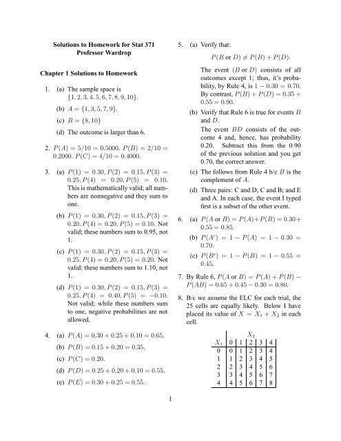
8. B/c we assume the ELC for each trial, the
25 cells are equally likely. Below I have
placed its value of X = X 1 + X 2 in each
cell.
X 2
X 1 0 1 2 3 4
0 0 1 2 3 4
1 1 2 3 4 5
2 2 3 4 5 6
3 3 4 5 6 7
4 4 5 6 7 8
1

Chapter 1 Solutions to Homework Continued
By counting:
x P(X = x) x P(X = x)
0 0.04 5 0.16
1 0.08 6 0.12
2 0.12 7 0.08
3 0.16 8 0.04
4 0.20
9. First, I note that the possible values of X =
X 1 +X 2 +X 3 are 3, 4, 5, 6, 7, 8 and 9. Also
note that the probabilitiy distribution for X
will be symmetric around 6. (Why?). Thus,
I need to determine only three probabilities.
P(X = 3) = P(1, 1, 1) = (1/3) 3 = 1/27.
P(X = 4) = 3P(1, 1, 2) = 3/27.
P(X = 5) = 3P(1, 1, 3)+3P(2, 2, 1) = 6/27.
Thus, the sampling distribution is:
x: 3 4 5 6
P(X = x): 1/27 3/27 6/27 7/27
x: 7 8 9
P(X = x): 6/27 3/27 1/27
10. First, we determine the probability of each
of the 16 cells.
11. The possible values of X are: 3, 4, . . . , 12.
Probabilities are given below.
P(X = 3) = P(1,1,1) = (0.1) 3 = 0.001.
P(X = 4) = 3P(1,1,2) = 3(0.1) 2 (0.2) = 0.006.
P(X = 5) = 3P(1,1,3) + 3P(1,2,2) =
3(0.1) 2 (0.3) + 3(0.1)(0.2) 2 = 0.021.
P(X = 6) = 3P(1,1,4)+6P(1,2,3)+P(2, 2, 2) =
3(0.1) 2 (0.4)+6(0.1)(0.2)(0.3)+(0.2) 3 = 0.056.
P(X = 7) = 6P(1,2,4)+3P(1,3,3)+3P(2,2,3) =
6(0.1)(0.2)(0.4)+3(0.1)(0.3) 2 +3(0.2) 2 (0.3) = 0.111.
P(X = 8) = 6P(1,3,4)+3P(2,2,4)+3P(2,3,3) =
6(0.1)(0.3)(0.4)+3(0.2) 2 (0.4)+3(0.2)(0.3) 2 = 0.174.
P(X = 9) = 3P(1,4,4)+6P(2,3,4)+P(3, 3, 3) =
3(0.1)(0.4) 2 +6(0.2)(0.3)(0.4)+(0.3) 3 = 0.219.
P(X = 10) = 3P(2,4,4) + 3P(3,3,4) =
3(0.2)(0.4) 2 + 3(0.3) 2 (0.4) = 0.204.
P(X = 11) = 3P(3,4,4) = 3(0.3)(0.4) 2 = 0.144.
P(X = 12) = P(4,4,4) = (0.4) 3 = 0.064.
12. (a) The approximation is 0.0854. The interval
is
√
0.0854±3 0.0854(0.9146)/10000 =
X 2
X 1 1 2 3 4
1 0.01 0.02 0.03 0.04
2 0.02 0.04 0.06 0.08
3 0.03 0.06 0.09 0.12
4 0.04 0.08 0.12 0.16
Summing probabilities, one gets the following
distribution for X.
x: 2 3 4 5
P(X = x): 0.01 0.04 0.10 0.20
x: 6 7 8
P(X = x): 0.25 0.24 0.16
0.0854 ± 0.0084 = [0.0770, 0.0938].
(b) P(X = 6) = 5P(1, 1, 1, 1, 2) =
0.000643. The approximation is
0.0002. The interval is
0.0002±0.0004 = [−0.0002, 0.0006].
(c) P(X = 28) = 5P(4, 6, 6, 6, 6) +
10P(5, 5, 6, 6, 6) = 0.001929. The
approximation is 0.0019. The interval
is
0.0019 ± 0.0013 = [0.0006, 0.0032].
2

Chapter 2 Solutions to Homework
1. (a) The probability of S, F, S, S, F , in
that order, is pqppq = p 3 q 2 =
(0.58) 3 (0.42) 2 = 0.0344.
(b) This will happen if Brian obtains
S, S, F , in that order. The probability
is ppq = (0.58) 2 (0.42) = 0.1413.
(c) This will happen if Brian begins with
three successes. The probability is
ppp = (0.58) 3 = 0.1951.
(d) The probability is P(X = 3) =
(e)
6!
3!3! (0.58)3 (0.42) 3 = 0.2891.
i. The probability of an Angelina is
P(X = 3) + P(X = 4) =
4!
3!1! (0.58)3 (0.42) + (0.58) 4 =
0.3278 + 0.1132 = 0.4410.
ii. The probability is P(X = 3) =
5!
3!2! (0.441)3 (0.559) 2 = 0.2680.
(f) Let X 1 denote the number of successes
Brian obtains on Saturday
morning and X 2 denote the number
of successes he obtains on Saturday
afternoon. Y = X 1 + X 2 .
i. P(Y = 7) =
The second of these is
5!
4!1! (0.58)4 (0.42)×
[ 4!
3!1! ((0.58)3 (0.42)] =
0.2376(0.3278) = 0.0779.
Thus, P(Y = 7) = 0.0163 +
0.0779 = 0.0942.
ii. P(Y = 3) =
P(X 1 = 2, X 2 = 1)+
P(X 1 = 3, X 2 = 0).
Now, the first of these is
5!
2!3! (0.58)2 (0.42) 3 ×
2!
1!1! (0.58)(0.42) =
0.2492(0.4872) = 0.1214.
The second of these is
5!
3!2! (0.58)3 (0.42) 2 ×
(0.42) 3 =
0.3442(0.0741) = 0.0255.
Thus, P(Y = 3) = 0.1214 +
0.0255 = 0.1469.
P(X 1 = 5, X 2 = 2)+
P(X 1 = 4, X 2 = 3).
Now, the first of these is
(0.58) 5 5!
2!3! (0.58)2 (0.42) 3 =
0.0656(0.2492) = 0.0163.
3

Chapter 2 Solutions to Homework Continued
(g) We cannot use the multiplication b/c
A and B are not independent b/c they
are both functions of the first and
last trials. So, we must be clever.
Define X to be the number of successes
on trials two thru seven. X ∼
Bin(6, 0.58). The event AB is the
same as the event BC where C is the
event that X = 4. Events B and C
are independent, so the answer is:
P(BC) = P(B)P(C) =
(.42) 2 6!
4!2! (0.58)4 (0.42) 2 =
0.1764(0.2994) = 0.0528.
2. For X ∼ Bin(1024, 0.50),
µ = np = 1024(0.50) = 512,
σ 2 = npq = 1024(0.50)(0.50) = 256, and
Thus,
σ = √ 256 = 16.
Z = X − 512 .
16
3. For X ∼ Bin(192, 0.25), µ = 48 and σ =
6. Thus, we enter the normal curve website
with these values.
(a) P(X ≥ 55): Enter 54.5 in the
‘Above’ box and obtain 0.1393.
(b) P(X = 48): Enter 47.5 and 48.5 in
the ‘Between’ box and obtain 0.0664.
(c) P(X ≤ 48): Enter 48.5 in the ‘Below’
box and obtain 0.5332.
(d) P(42 ≤ X ≤ 60): Enter 41.5 and
60.5 in the ‘Between’ box and obtain
0.8421.
(e) P(45 ≤ X < 57): Enter 44.5 and
56.5 in the ‘Between’ box and obtain
0.6419.
4. (a) 0.1398.
(b) 0.0664. (Thus, the approximation is
correct.)
(c) 0.5387.
(d) 0.9795 − 0.1387 = 0.8408.
(e) 0.9199 − 0.2830 = 0.6369.
5. Below are all the ones I could figure out:
P(X ≥ 94) = 1 − 0.2277 = 0.7723.
P(94 ≤ X ≤ 100) = 0.5268−0.2277 = 0.2991.
P(X ≤ 93 or X ≥ 101) =
1 − 0.2991 = 0.7009.
6. P(X ≥ 4) = P(X = 4) + P(X = 5) +
P(X = 6) + P(X = 7) =
7!
4!3! (0.50166)4 (0.49834) 3 +
7!
5!2! (0.50166)5 (0.49834) 2 +
7!
6!1! (0.50166)6 (0.49834)+
7!
7!0! (0.50166)7 =
0.2743+0.1657+0.0556+0.0080 = 0.5036.
7. First, µ = 801(0.50166) = 401.83 and σ =
14.151. Enter 400.5 in the ‘Above’ box of
the normal curve website; the approximate
answer is 0.5365. Thus, even with a sample
of size 801 a projection is barely better than
tossing a coin.
4

Chapter 3 Solutions to Homework
1. First, ˆp = 220/400 = 0.55 and ˆq = 1 −
0.55 = 0.45. Next,
√ √
(ˆpˆq)/n = (0.55)(0.45)/400 = 0.02487.
Thus, the CIs are:
0.550±1.645(0.02487) = 0.550±0.041 =
[0.509, 0.591].
0.550 ± 1.96(0.02487) = 0.550 ± 0.049 =
[0.501, 0.599].
0.550±2.576(0.02487) = 0.550±0.064 =
[0.486, 0.614].
2. First, ˆp = 880/1600 = 0.55 and ˆq = 1 −
0.55 = 0.45. Next,
√ √
(ˆpˆq)/n = (0.55)(0.45)/1600 = 0.01244.
Thus, the CIs are:
0.550 ± 1.645(0.0124) = 0.550 ± 0.020 =
4. (a) [0.000, 0.190].
(b) [0.000, 0.151].
(c) [0.000, 0.269].
5. We are given that
Thus,
√
0.03925 = 1.282 ˆpˆq/n;
√
ˆpˆq/n = 0.03925/1.282 = 0.03062.
Thus, the CIs are ˆp±
6. From above,
1.645(0.03062) = 0.05036;
1.96(0.03062) = 0.06001; and
2.326(0.03062) = 0.07122.
0.03062 =
√
0.25(0.75)/n.
Square both sides and solve for n. The result
is n = 200.
[0.530, 0.570].
0.550 ± 1.96(0.01244) = 0.550 ± 0.024 =
[0.526, 0.574].
0.550±2.576(0.01244) = 0.550±0.032 =
[0.518, 0.582].
With ˆp unchanged, the effect of a four-fold
increase in n is that each CI becomes onehalf
as wide.
3. Below are the CIs; in each case the 90% is
listed first.
(a) [0.131, 0.406]; [0.115, 0.434].
(b) [0.164, 0.355]; [0.150, 0.374].
(c) [0.483, 0.723]; [0.461, 0.742].
5

Chapter 3 Solutions to Homework Continued
7. (a) By trial-and-error I find that for x ≤
19 the CI is too small (its upper bound
is < 0.45); for x ≥ 35 the CI is
too large (its lower bound is > 0.45).
Thus, the CI is correct if, and only if,
20 ≤ x ≤ 34.
(b) Going to the website for binomial
probabilities, we find that for n = 60
and p = 0.45:
P(X ≤ 34) − P(X ≤ 19) =
0.9739 − 0.0246 = 0.9493,
which is very close to the target of
0.95.
8. (a) By trial-and-error I find that for x ≤ 6
the CI is too small (its upper bound is
< 0.30); for x ≥ 19 the CI is too large
(its lower bound is > 0.30). Thus, the
CI is correct if, and only if, 7 ≤ x ≤
18.
(b) Going to the website for binomial
probabilities, we find that for n = 40
and p = 0.30:
P(X ≤ 18) − P(X ≤ 6) =
0.9852 − 0.0238 = 0.9614,
which is ≥ 0.95, as promised.
6

Chapter 4 Solutions to Homework
1. The mean is θ = 49. The variance is θ =
49. The standard deviation is √ θ = √ 49 =
7.
2. For (a)–(c) go to the website and type 20
for both x and the average rate of success.
(a) P(X = 20) = 0.0888.
(b) P(X ≤ 20) = 0.5591.
(c) P(X > 20) = 0.4409.
(d) There are several ways to get the answer.
I suggest:
P(16 ≤ X ≤ 24) =
P(X ≤ 24) − P(X ≤ 15).
We will need to use the website twice;
we get 0.8432 − 0.1565 = 0.6867.
3. In order to use the normal curve, we need to
remember that for the Poisson, µ = θ and
σ = √ θ. Thus, for this problem, µ = 64
and σ = 8.
(a) Using the normal curve with the continuity
correction, we write
P(X > 75) = P(X ≥ 75.5).
This is approximated by the area under
our normal curve above 75.5,
which is 0.0753.
The website easily gives us the exact
probability: enter 75 for x and 64 for
the average rate of success; the answer
is 0.0781. The approximation is
pretty good.
(b) First write
This is approximated by 0.4232
We must use the website twice to get
the exact answer. I type in 70 and then
60 for x, using 64 for the average rate
of success both times. The result is
0.7576 − 0.3371 = 0.4205. The approximation
is pretty good.
4. (a) For 98%, z = 2.326. Thus, the snc CI
for θ is
72 ± 2.326 √ 72 = 72 ± 19.74 =
[52.26, 91.74].
(b) The exact CI is [53.74, 94.33]. This
typically happens; the approximation,
compared to the exact, makes the
lower and upper bounds smaller.
5. As discussed in the Course Notes, Tim’s θ
is the product of rate and time: 5(4.5) =
22.5. We obtain P(X = 26) = 0.0602.
6. Now Tim has observed the process for
4.5 + 1.75 = 6.25 hours. The θ is now
5(6.25) = 31.25. We find P(Y ≤ 30) =
0.4583.
7. The 95% exact CI for θ is [28.58, 54.47].
This is the CI for 6.25 times the rate. In
symbols, the CI asserts:
28.58 ≤ 6.25(rate) ≤ 54.47.
Dividing thru by 6.25 gives 28.58/6.25 =
4.57 and 54.47/6.25 = 8.72. Thus,
[4.57, 8.72] is the 95% CI for the rate; b/c
the rate is 5, the CI is correct.
P(60 < X < 70) =
P(60.5 < X < 69.5) =
7

Chapter 5 Solutions to Homework
1. (a) Type 5 into the df box and 12 into the
box on the lower left. The answer is
0.0348.
(b) Type 8 into the df box and 16.721 into
the box on the lower left. The answer
is 0.0332.
(c) Type 10 into the df box and 21.12 into
the box on the lower left. The answer
is 0.0203.
2. (a) Type 10 into the df box and 0.01 into
the box on the lower right. The answer
is 23.21.
(b) Type 11 into the df box and 0.05 into
the box on the lower right. The answer
is 19.68.
(c) Type 9 into the df box and 0.10 into
the box on the lower right. The answer
is 14.68.
3. (Optional problem.) There are many possible
correct answers.
4. The critical region is χ 2 ≥ χ 2 0.01 (5) =
15.09.
B/c I am lazy, I typed my O’s and hypothesized
probabilities (all 1/6) into the Goodness
of Fit calculator on the web. I obtained
χ 2 = 51.94 with df = 5. This website also
tells me that the P-value is < 0.0001. B/c
51.94 > 15.09 my decision is to reject the
null hypothesis and conclude that, like my
blue die, my white die is not balanced and
fair.
For practice you should calculate a few values
of (O − E) 2 /E. Remember, each E
equals 1000(1/6) = 166.7.
5. First, the hypothesized probabilities are a,
2a and a. B/c these sum to one, a = 0.25.
The null hypothesis states that the probability
of black is 0.25, the probability of
brown is 0.50 and the probability of white
is 0.25.
For α = 0.05 the critical region is
χ 2 ≥ χ 2 0.05(2) = 5.991.
Next, n = 40 + 59 + 42 = 141, giving E’s
of 35.25, 70.50 and 35.25. Below are the
details for the computation of χ 2 .
Outcome Black Brown White
O i 40 59 42
E i 35.25 70.50 35.25
O i − E i 4.75 −11.50 6.75
(O i − E i ) 2 22.56 132.25 45.56
(O i − E i ) 2 /E i 0.640 1.876 1.292
Summing the values in the last row, I get
χ 2 = 3.808, so I fail to reject the null. Going
to the Chi-Squared area calculator, the
P-value is found to be 0.149.
6. This is similar to the hypothetical example
of Bob shooting in the Lecture Examples.
First, we need to estimate p. Bird attempted
2(338) = 676 free throws and achieved
0(5) + 1(82) + 2(251) = 584
successes. Thus, ˆp = 584/676 = 0.8639.
With this estimate of p, we can obtain the
estimated E’s:
E 0 = 338P(X = 0) = 338(0.1361) 2 =
338(0.01852) = 6.26.
E 1 = 338P(X = 1) = 338(2)(0.8639)(0.1361) =
338(0.2352) = 79.5.
E 2 = 338P(X = 2) = 338(0.8639) 2 ) =
338(0.7463) = 252.3.
8

Chapter 5 Solutions to Homework Cont.
The approximating curve will be χ 2 (k−1−
1) = χ 2 (1). At the Chi-Squared calculator,
I type 1 in the degrees of freedom box and
0.10 in the lower right box. I click on the
compute button and learn that χ 2 0.10 (1) =
2.706. Thus, the critical region for my test
is χ 2 ≥ 2.706.
Below are my computations for the observed
value of the test statistic.
O i 5 82 251
E i 6.26 79.5 252.3
O i − E i −1.26 2.5 −1.3
(O i − E i ) 2 1.588 6.25 1.69
(O i − E i ) 2 /E i 0.254 0.079 0.007
Summing the numbers in the last row, I obtain
χ 2 = 0.340. Thus, I fail to reject the
null. The P-value is 0.5598.
9

Chapter 6 Solutions to Homework
1. (a) Below is the 4 × 2 table.
Quarter S F Total ˆp
1st 35 15 50 0.70
2nd 29 21 50 0.58
3rd 21 29 50 0.42
4th 16 34 50 0.32
Using the Chi-Squared site, we find
that χ 2 = 17.022 with r − 1 = 4 −
1 = 3 degrees of freedom, giving a P-
value of 0.0007. There is very strong
evidence in support of changing p and
I reject the null hypothesis of constant
p.
(b) Below is the 2 × 2 table.
Half S F Total ˆp
1st 64 36 100 0.64
2nd 37 63 100 0.37
Using the Fisher’s test, we find a P-
value of 0.0002. There is very strong
evidence in support of changing p and
I reject the null hypothesis of constant
p.
(c) Below is the memory table.
Current
Previous S F Total ˆp
S 53 48 101 0.52
F 47 51 98 0.48
Total 100 99 199
Fisher’s test gives a P-value of
0.5717.
(d) Our examinations in (a) and (b) both
detected the changing p.
Using the Chi-Squared site, we find
that χ 2 = 5.269 with r−1 = 4−1 = 3
degrees of freedom, giving a P-value
of 0.1531. There is some evidence in
support of changing p, but not enough
to reject the null hypothesis of constant
p.
(b) Below is the 2 × 2 table.
Half S F Total ˆp
1st 58 42 100 0.58
2nd 55 45 100 0.55
Using the Fisher’s test, we find a P-
value of 0.7755. There is very weak
evidence in support of changing p and
I do not reject the null hypothesis of
constant p.
(c) Below is the memory table.
Current
Previous S F Total ˆp
S 64 49 113 0.57
F 49 37 86 0.57
Total 113 86 199
Fisher’s test gives a P-value of 1.
(d) Our examinations in (a) and (b) both
failed to detect the changing value of
p.
2. (a) Below is the 4 × 2 table.
Quarter S F Total ˆp
1st 34 16 50 0.68
2nd 24 26 50 0.48
3rd 30 20 50 0.60
4th 25 25 50 0.50
10

Chapter 6 Solutions to Homework Cont.
3. (a) Below is the 6 × 2 table.
Sixth S F Total ˆp
1st 15 12 27 0.556
2nd 16 11 27 0.593
3rd 12 15 27 0.444
4th 11 16 27 0.407
5th 11 16 27 0.407
6th 15 12 27 0.556
Using the Chi-Squared site, we find
that χ 2 = 3.754 with r−1 = 6−1 = 5
degrees of freedom, giving a P-value
of 0.5853. There is very weak evidence
in support of changing p; not
nearly enough to reject the null hypothesis
of constant p.
(b) Below is the 3 × 2 table.
Third S F Total ˆp
1st 31 23 54 0.574
2nd 23 31 54 0.426
3rd 26 28 54 0.481
Using the Chi-Squared site, we find
that χ 2 = 2.42 with r −1 = 3−1 = 2
degrees of freedom, giving a P-value
of 0.2982. There is some evidence in
support of changing p, but not nearly
enough to reject the null hypothesis of
constant p.
(c) Below is the 2 × 2 table.
Half S F Total ˆp
1st 43 38 81 0.531
2nd 37 44 81 0.457
Using the Fisher’s test, we find a P-
value of 0.4321. There is only weak
evidence in support of changing p.
(d) Below is the memory table.
Current
Previous S F Total ˆp
S 39 40 79 0.494
F 41 41 82 0.500
Total 80 81 161
Fisher’s test gives a P-value of 1.
4. (a) Below is the 4 × 2 table.
Quarter S F Total ˆp
1st 19 6 25 0.76
2nd 9 16 25 0.36
3rd 11 14 25 0.44
4th 8 17 25 0.32
Using the Chi-Squared site, we find
that χ 2 = 12.003 with r − 1 = 4 −
1 = 3 degrees of freedom, giving a P-
value of 0.0074. There is very strong
evidence in support of changing p and
I reject the null hypothesis of constant
p.
(b) Below is the 2 × 2 table.
Quarter S F Total ˆp
1st 28 22 50 0.56
2nd 19 31 50 0.38
Using Fisher’s test we find a P-value
of 0.1085.
(c) Below is the memory table.
Current
Previous S F Total ˆp
S 26 20 46 0.57
F 20 33 53 0.38
Total 46 53 99
The P-value, 0.0717, just barely fails
to achieve statistical significance.
5. Table 1 is correct for (b) and (e); Table 2 is
correct for (c) and (f); Table 3 is correct for
(a), (d) and (g).
11

Chapter 7 Solutions to Homework
1. These are BT with p known to equal 3/16
and m = 800. To obtain the point prediction,
we begin by calculating mp =
800(3/16) = 150. B/c this is an integer it
is our point prediction. The 90% prediction
interval is 150±
√
1.645 150(13/16) = 150±1.645(11.04) =
150 ± 18.2 = [132, 168].
2. These are BT with p known to equal 9/16
and m = 320. To obtain the point prediction,
we begin by calculating mp =
320(9/16) = 180. B/c this is an integer it
is our point prediction. The 95% prediction
interval is 180±
√
1.96 180(7/16) = 150 ± 1.96(8.87) =
180 ± 17.4 = [163, 197].
3. (a) These are BT with p unknown. Our
past data are n = 736 and x = 511,
which give ˆp = 511/736 = 0.694. To
obtain the point prediction, we begin
by calculating mˆp = 695(0.694) =
482.3. B/c this is not an integer,
our ad-hoc point prediction is 482.
(Rounding to 483 is ok too.)
The 80% prediction interval is
482.3±
√ √
1.282 482.3(0.306) 1 + (695/736) =
(b) The point prediction is too small by
34 and the prediction interval also is
incorrect. (BTW, the 95% prediction
interval would have 515.5 for its
upper bound before rounding. After
rounding to 516 it would be barely
correct, but correct.)
4. (a) First, ˆp = 49/480 = 0.102 The snc
approximation gives
√
0.102 ± 1.96 0.102(0.898)/480 =
0.102±1.96(0.0138) = 0.102±0.027 =
[0.075, 0.129]. BTW, the exact CI is
[0.076, 0.132], which is very close to
the snc answer.
(b) First, ˆp = 73/476 = 0.153 The snc
approximation gives
√
0.153 ± 1.96 0.153(0.847)/476 =
0.153±1.96(0.0165) = 0.153±0.032 =
[0.121, 0.185]. BTW, the exact CI is
[0.122, 0.189], which is very close to
the snc answer. Note that whether you
use the approximate or exact method,
the CI’s from (a) and (b) overlap.
482.3 ± 1.282(12.15)(1.394) =
482.3 ± 21.7 = [460, 6, 504.0] =
[461, 504], after rounding.
We assume that each year Malone’s
shots were BT with the same p for
both years.
12

Chapter 7 Solutions to Homework Cont.
(c) These are BT with p unknown. Our
past data are n = 480 and x = 49,
which give ˆp = 0.102. To obtain the
point prediction, we begin by calculating
mˆp = 476(0.102) = 48.6. B/c
this is not an integer, our ad-hoc point
prediction is 49. (Rounding to 48 is
ok too.)
The 98% prediction interval is 48.6±
√ √
2.326 48.6(0.898) 1 + (476/480) =
(b) For this part, c 1 = 160 and c 2 = 74,
giving c = 74/160 = 0.4625. Also,
x = 163. Thus, cx = 75.4. The 95%
prediction interval is 75.4±
√
1.96 75.4(1 + 0.4625) =
75.4 ± 1.96(10.50) =
75.4 ± 20.6 = [55, 96],
after rounding.
The PI is correct b/c it includes 87.
48.6 ± 2.326(6.06)(1.411) =
48.6 ± 21.7 = [26.9, 70.3] =
[27, 70], after rounding.
Obviously, the point prediction was
much too small and the prediction interval
is incorrect too. But I conjecture
that most baseball fans would be
amazed with the width of this interval.
Yes, BB (and hundreds of others)
probably used steroids, but his 73
home runs was not that far away from
the variation in BT.
5. Refer to page 76 in the Course Notes.
Remember that c 1 is the number of past
games, c 2 is the number of games we want
to predict and c = c 2 /c 1 .
(a) For this part, c 1 = c 2 = 80; thus, c =
1. Also, x = 92. The 90% prediction
interval is 92±
√
1.645 92(1 + 1) = 92±1.645(13.56) =
after rounding.
92 ± 22.3 = [70, 114],
The PI is correct b/c it includes 71, but
it is barely correct.
13

Chapter 9 Solutions to Homework
1. (a) First, ˆp 1 = 251/285 = 0.881 and
ˆp 2 = 48/53 = 0.906. The 95% CI
is (0.881 − 0.906)±
1.96
√
0.881(0.119)
285
+ 0.906(0.094)
53
−0.025±1.96(0.0444) = −0.025±0.087 =
[−0.112, 0.062].
We must assume independent BT for
each row of data.
(b) From the website, the exact P-value is
0.8149. The evidence for the alternative
is very weak. Even with the alternative

Chapter 9 Solutions to Homework Cont.
(a) First, ˆp 1 = 305/376 = 0.811 and
ˆp 2 = 97/133 = 0.729. The 95% CI is
(0.811 − 0.729)±
1.96
√
0.811(0.189)
376
+ 0.729(0.271)
133
0.082±1.96(0.0435) = 0.082±0.085 =
[−0.003, 0.167].
We must assume independent BT for
each row of data. When you recall
that the data in each row is a mixture
of two players and that one player has
a much larger p than the other player,
this makes no sense. Furthermore,
row two has much more of its data
from the worse shooter! But, in my
experience, often people find data and
just analyze it without thinking. So
if someone says, “Here are some data
on free throw shooting in the NBA;
what do you think?” It takes some
intellectual courage to reply, “I need
more information.”
(b) From the website, the exact P-value
is 0.0627. For the alternative >, the
exact P-value is 0.0326.
For the approximate test, begin with
ˆp = 402/509 = 0.790. The observed
value of the test statistic is
z =
=
0.082
√[(0.79)(0.21)](1/376 + 1/133) =
For α = 0.10 the decision is to reject
b/c the P-value is less than or equal to
0.10.
(c) In both component tables (tables for
individual players) ˆp 1 < ˆp 2 , but in the
collapsed table, ˆp 1 > ˆp 2 . This reversal
is Simpson’s Paradox.
5. B/c both PP’s are observed for the same
length of time (number of games, 80), c =
1 and our formulas simplify.
(a) The 98% CI for (θ 1 − θ 2 ) is
(x − y) ± 2.326 √ x + y =
(92−71)±2.326 √ 92 + 71 = 21±29.70 =
[−8.70, 50.70]. Next, dividing each
endpoint by 80, we get the CI for
(λ1 − λ2):
[−0.109, 0.634].
(b) The observed value of the test statistic
is
z = (x − y)/ √ x + y = 21/ √ 163 =
1.645. The area under the snc to the
right of |z| = 1.645 is 0.05; doubling
this, we get an approximate P-value
of 0.10.
For α = 0.05 the decision is to fail
to reject b/c the P-value is larger than
0.05.
0.082/0.0411 = 1.995.
The area under the snc to the right
of |z| = +1.995 is 0.0230; doubling
this, we get an approximate P-value
of 0.0460. This is a bad approximation
to 0.0627.
15

Chapter 10 Solutions to Homework
1. (a) 4.
(b) It is impossible for a relative frequency
to exceed 1.
(c) The area of the rectangle is 0.1(4) =
0.4. Thus, the relative frequency of
the interval is 0.4. The frequency is
the product of the relative frequency
and n: 0.4(200) = 80.
2. (a) The median is the average of the observations
in positions 25 and 26:
(3.01 + 3.18)/2 = 3.095.
(b) First, we create the table:
14
Class
Interval Frequency
0.00–1.00 14
1.00–2.00 4
2.00–3.00 6
3.00–4.00 8
4.00–5.00 18
Total 50
4 6 8
18
this interval. Thus, 25, or 50%, of
the data are in the interval. This is
much smaller than the 68% predicted
by the empirical rule. This is no surprise
b/c our histogram has two separated
peaks.
4. (a) The interval is [17.56−13.23, 17.56+
2(13.23)] = [4.33, 44.02]. By counting,
1 observation is too small and 3
observations are too large to be in this
interval. Thus, 29 observations, or
88% of the data, are in the interval.
(b) The median is the number in position
17: 12.64. Next, 0.25(33) = 8.25,
which we round up to 9. Thus, Q 1 =
7.57. And 0.75(33) = 24.75, which
we round up to 25. Thus, Q 3 = 21.50.
(c) To find Q 1 we still count to position
9, remembering that the data have
changed; we get 8.27. The median
is still in position 17, which is now
13.59. The mean is a bit trickier.
We have increased the total of the 33
observations by 10, so the mean increases
by 10/33 = 0.30, giving us a
new mean of 17.86.
0 1 2 3 4 5
(c) Go to next page for solution.
3. (a) First, 0.25(n) = 12.5, which we
round up to 13; 0.75(n) = 37.5,
which we round up to 38. Thus, Q 1 =
0.93 and Q 3 = 4.45.
(b) The interval ¯x ± s = 2.76 ± 1.78 =
[0.98, 4.54]. By counting, 13 observations
are too small to be in this interval
and 12 are too large to be in
16

Chapter 10 Solutions to Homework Cont.
2. (Cont.) (c) First, we create the table:
Class Width Frequency Relative Freq. Density
Interval (w) (freq) rf = (freq/n) (rf/w)
0.00–0.50 0.5 11 0.22 0.44
0.50–2.50 2.0 8 0.16 0.08
2.50–4.50 2.0 19 0.38 0.19
4.50–5.00 0.5 12 0.24 0.48
Total —- n = 50 1.00 —-
0.44
0.48
0.19
0.08
0 1 2 3 4 5
17

Chapter 11 Solutions to Homework
1. (a) First, we note that df = n − 1 = 39.
From the online calculator, for the
95% CI, t = 2.023. For future use,
note that 29.87/ √ 40 = 4.7229. Thus,
the CI is
106.87 ± 2.023(4.7229) =
106.87 ± 9.55 = [97.32, 116.42].
(b) From the online calculator, for the
99% CI, t = 2.708. Thus, the CI is
106.87 ± 2.708(4.7229) =
106.87 ± 12.79 = [94.08, 119.66].
(c) The observed value of the test statistic
is
t =
106.87 − 100
4.7229
= 1.455.
From the online calculator, the area
under the t(39) curve to the right of
1.455 is 0.0768; this is the approximate
P-value.
(d) The observed value of the test statistic
is
t =
106.87 − 120
4.7229
= −2.780.
From the online calculator, the area
under the t(39) curve to the left of
−2.780 is 0.0042; this is the approximate
P-value.
(e) We note that 95% gives z = 1.96.
Thus,
k ′ = 41 2 − 1.96√ 40
2
= 20.5 −6.20 =
14.30. We round k ′ down to k =
14. The 14th smallest observation is
107 and the 14th largest observation
is 122. Thus, the CI is [107, 122].
2. (a) First, we note that df = n − 1 =
14. From the online calculator, for
the 90% CI, t = 2.023. For future
use, note that 0.3253/ √ 15 = 0.0840.
Thus, the CI is
7.10 ± 1.761(0.0840) =
7.10 ± 0.15 = [6.95, 7.25].
(b) From the online calculator, for the
98% CI, t = 2.624. Thus, the CI is
7.10 ± 2.624(0.0840) =
7.10 ± 0.22 = [6.88, 7.32].
(c) The observed value of the test statistic
is
t =
7.10 − 7.00
0.0840
= 1.191.
From the online calculator, the area
under the t(14) curve to the right of
1.191 is 0.1267; this is the approximate
P-value.
(d) The observed value of the test statistic
is
t =
7.10 − 7.20
0.0840
= −1.191.
From above, the area under the t(14)
curve to the right of |t| = 1.191 is
0.1267; twice this, 0.2534, is the approximate
P-value.
(e) Because n < 21 we can use the table
from our ‘Tables’ section of the
course webpage to obtain the exact
CI. From the table, the possibilities
for the confidence level are 99.3%,
96.5% and 88.2%. The last of these
is the closest to 90%. The 88.2% CI
is
x (5) , x (11) ] = [6.88, 7.23].
18

Chapter 11 Solutions to Homework Cont.
3. (a) None of the lower bounds is > 90;
thus, none of the CI’s is too large.
One upper bound, 82, is < 90; thus,
one of the CI’s is too small. B/c one
CI is incorrect, the other three must be
correct. Or, by examination, 90 is not
in the first CI, but is in the other 3.
(b) With problems like this, you must
save determining the correct intervals
until the end. It does not matter
whether you begin with too small or
too large intervals.
One interval is too small, which
means that one upper bound is too
small. The smallest upper bound is
82; thus,
82 < µ.
One interval is too large, which means
that one lower bound is too large. The
largest lower bound is 86; thus,
µ < 86.
The remaining two CI’s must be the
correct one. Thus, in addition to the
two inequalities displayed earlier, we
have
49 ≤ µ ≤ 92 and 57 ≤ µ ≤ 95.
Finally, you apply the logic of ‘and’
which tells us that µ must be > 82
and < 86. Thus, the answer is
82 < µ < 86.
(c) This solution illustrates a useful technique.
Begin with any candidate for
µ that is smaller than every lower
bound, say 0. If µ = 0 then there are
no correct CI’s. As µ moves to the
right there will continue to be no correct
CI’s until a lower bound is met.
The smallest lower bound is 43, so at
µ = 43 there will be one correct CI.
This will continue until µ gets to 49
at which point a second CI will become
correct. For a very long time,
there will remain 2 or more correct
CI’s. But when µ crosses 95 the first
three CI’s will be too small and only
the last CI will be correct. This last CI
will remain correct until µ crosses its
upper bound, 112. Thus, the answer
is
43 ≤ µ < 49 or 95 < µ ≤ 112.
4. (a) Nine CI’s are too large; one CI is too
small. Thus, 18 − 9 − 1 = 8 CI’s are
correct.
(b) Well, 393 and 409 are too large, but
375 is not too large. Thus, 375 ≤ µ <
393.
(c) All we know is that the upper bounds
351 and smaller are all too small.
Thus, 351 < µ.
(d) The technique is similar to what we
used in answering 3(c). In order to
have 11 correct CI’s µ must have ‘entered’
at least 11 CI’s. Thus, we begin
our search at the 11th lower bound,
308. But at 308, one CI is too small
(the one with upper bound at 294), so
there are only 10 correct CI’s. Thus,
we move to the next lower bound,
322, and find that at 322 there is one
CI that is too small, so there are 11
correct CI’s. This remains true until
we cross 326 when another CI becomes
too small and the number of
correct CI’s decreases to 10 again. We
can summarize this line of reasoning
with the following table.
19

Chapter 11 Solutions to Homework Cont.
L 308 322 334 344 360 375
A 11 12 13 14 15 16
B 1 1 3 3 5 8
Corr 10 11 10 11 10 8
In this table, the L’s are consecutive
lower bounds beginning at 308 b/c, as
noted above, we cannot possibly have
11 correct CI’s for µ < 308. An A is
the position of an L in the list; it is the
maximum number of CI’s that could
be correct at µ = L. Next, B is the
number of CI’s that are too small at
µ = L. Finally, ‘Corr’ equals A − B
is the number actually correct at L.
I stopped my listing at 375 b/c with
only 8 correct CI’s we will never get
back up to 11 correct again as we
travel to the right. We see that 11 correct
occurs at 322 and 344. Finally,
we must remember that the number
of correct remains constant until we
cross an upper bound. Thus, all µ’s
that give 11 correct are:
322 ≤ µ ≤ 326 or 344 ≤ µ ≤ 345.
20

Solutions to Chapter 12 Homework
1. (a) With n = 33, df = n − 1 = 32. From
the calculator, the t for the 95% CI is
t = 2.037. Thus, the CI is
0.52 ± 2.037(0.733/ √ 33) =
0.52 ± 2.037(0.1276) =
0.52 ± 0.26 = [0.26, 0.78].
(b) With n = 34, df = n − 1 = 33. From
the calculator, the t for the 95% CI is
t = 2.035. Thus, the CI is
0.04 ± 2.035(0.744/ √ 34) =
0.04 ± 2.035(0.1276) =
0.04 ± 0.26 = [−0.22, +0.30].
(c) B/c both n 1 and n 2 exceed 19, we use
Case 3. First, we calculate
√
(0.733)
2
33
+ (0.744)2
34
= 0.1804.
The observed value of the test statistic
is
z =
0.52 − 0.04
0.1804
= 2.660.
From the calculater, the area under the
snc to the right of 2.660 is 0.0039;
double this to get the P-value for the
third alternative: 0.0078.
(d) We use the calculation of the big
square root from (c). This gives us
0.48 ± 1.96(0.1804) = 0.48 ± 0.35 =
2. (a) With n = 20, df = n − 1 = 19. From
the calculator, the t for the 98% CI is
t = 2.539. Thus, the CI is
45.7 ± 2.539(22.74/ √ 20) =
45.7 ± 2.539(5.0848) =
45.7 ± 12.9 = [32.8, 58.6].
(b) The observed value of the test statistic
is
t =
45.7 − 40.5
5.0848
= 1.023.
Using the calculator, the area under
the t(19) curve to the right of 1.023
is 0.1596; this is our P-value.
3. (a) Put 16 in the top box; select the option
‘Area right of;’ enter 0.10 in the right
box; and click on ‘Compute!’ The answer
is t = 1.337.
(b) Put 31 in the top box; select the option
‘Area right of;’ enter 0.025 in the right
box; and click on ‘Compute!’ The answer
is t = 2.04.
(c) Put 18 in the top box; select the option
‘Area right of;’ enter 2.105 in the left
box; and click on ‘Compute!’ The P-
value is 0.0248.
(d) Put 32 in the top box; select the option
‘Area right of;’ enter 3.011 in the left
box; and click on ‘Compute!’ The P-
value is twice the number displayed:
2(0.0025) = 0.0050.
(e) Put 33 in the top box; select the option
‘Area left of;’ enter −1.875 in the left
box; and click on ‘Compute!’ The P-
value is 0.0348.
[0.13, 0.83].
21

Chapter 12 Solutions to Homework Cont.
4. (a) First, df = 17, giving t = 2.11 for the
95% CI. Second, ¯x − ȳ = 4.50. Next,
s 2 p = 6(6.5)2 + 11(4) 2
6 + 11
= 25.2647.
Thus, s p = 5.026. The 95% CI is
√
4.50 ± 2.11(5.026) 1/7 + 1/12 =
4.50 ± 2.11(2.391) = 4.50 ± 5.04 =
[−0.54, 9.54].
The observed value of the test statistic
is
t = 4.50/2.391 = 1.882.
Finally, we go to the t-calculator and
enter 17 in the top box, 1.882 in
the left box and select ‘Area right
of.’ The result, in the right box, is
0.0385. Therefore, the P-value for
> is 0.0385; the P-value for < is
1 − 0.0385 = 0.9615; and the P-value
for ≠ is 2(0.0385) = 0.0770.
(b) First, df = 21, giving t = 2.08 for the
95% CI. Second, ¯x − ȳ = 1.20. Next,
s 2 p = 16(11.5)2 + 5(14) 2
16 + 5
= 147.43.
Thus, s p = 12.14. The 95% CI is
√
1.20 ± 2.08(12.14) 1/17 + 1/6 =
Finally, we go to the t-calculator and
enter 21 in the top box, 0.208 in
the left box and select ‘Area right
of.’ The result, in the right box, is
0.4186. Therefore, the P-value for
> is 0.4186; the P-value for < is
1 − 0.4186 = 0.5814; and the P-value
for ≠ is 2(0.4186) = 0.8372.
(c) First, df = 27, giving t = 2.052 for
the 95% CI. Second, ¯x − ȳ = −8.90.
Next,
s 2 p = 18(21.5)2 + 9(18.2) 2
18 + 9
= 418.58.
Thus, s p = 20.46. The 95% CI is
√
−8.90±2.052(20.46) 1/19 + 1/10 =
−8.90±2.052(7.993) = −8.90±16.40 =
[−25.30, 7.50].
The observed value of the test statistic
is
t = −8.90/7.993 = −1.114.
Finally, we go to the t-calculator and
enter 27 in the top box, −1.114 in
the left box and select ‘Area left
of.’ The result, in the right box, is
0.1375. Therefore, the P-value for
< is 0.1375; the P-value for > is
1 − 0.1375 = 0.8625; and the P-value
for ≠ is 2(0.1375) = 0.2750.
1.20 ± 2.08(5.766) = 1.20 ± 11.99 =
[−10.79, 13.19].
The observed value of the test statistic
is
t = 1.20/5.766 = 0.208.
22

Solutions to Chapter 13 Homework
1. (a) 453/3614 = 0.125
(b) 3325/3614 = 0.920
(c) 3126/3614 = 0.865
(d) 254/3614 = 0.070
(e) 35/3161 = 0.011
(f) 199/3325 = 0.060
(g) (254 + 3126)/3614 = 0.935
(h) 199/(35 + 199) = 0.850
(i) (3614 − 254)/3614 = 0.930
2. (a) The table is below.
Don’t
Drive Drive Total
Female 126 378 504
Male 234 162 396
Total 360 540 900
(b) The table is below.
Don’t
Drive Drive Total
Female 0.14 0.42 0.56
Male 0.26 0.18 0.44
Total 0.40 0.60 1.00
(b) We need (b − c) = 25 − 62 = −37
and (b+c) = 25+62 = 87. The 90%
CI is
( −37
400 )±1.645 √ √√√
400(87) − (−37) 2
399(400) 2 =
−0.0925 ± 1.645(0.0229) =
−0.0925 ± 0.0376 =
[−0.1301, −0.549].
4. (a) We go to the website and enter 0.5 in
the first box; 142 in the second box;
85 in the third box; and click on ‘Calculate.’
The P-values are 0.0116 for
>; 0.9927 for ;
0.000045 for