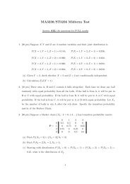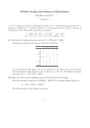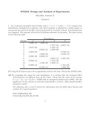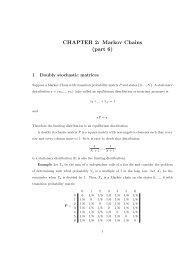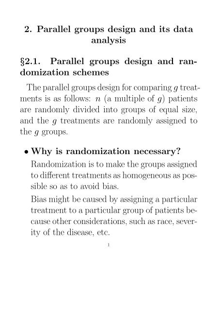
2. Parallel groups design and its data analysis §2.1. Parallel groups ...

2. Parallel groups design and its data
analysis
§2.1. Parallel groups design and randomization
schemes
The parallel groups design for comparing g treatmentsisasfollows:
n (a multiple of g) patients
are randomly divided into groups of equal size,
and the g treatments are randomly assigned to
the g groups.
• Why is randomization necessary?
Randomization is to make the groups assigned
to different treatments as homogeneous as possible
so as to avoid bias.
Bias might be caused by assigning a particular
treatment to a particular group of patients because
other considerations, such as race, severity
of the disease, etc.
1

When bias presents the treatment effects will
be confounded with the effects of other (unknown)
factors.
• Simple randomization scheme and its
drawbacks
A simple randomization scheme is obtained by
randomly permute the n patients and then
divide the permute patients in order into g
groups.
An example: 45 patients are randomly permuted
and divided into 3 groups.
44 42 10 21 28 38 6 31 27 30 17 35 29 41 15
9 25 14 16 37 45 40 36 8 24 32 5 20 34 2
33 43 13 23 12 4 1 3 18 22 11 26 19 7 39
If the trials stops earlier than planned, it might
result in an imbalance of patients among the
groups, some bias might occur.
2

• Randomly permuted blocks schemes
Instead of permuting all patients together, patients
are permuted in batches with size as a
smaller multiple of g.
The simplest one is to permute the patients in
batches of size g.
— This scheme is easier to implement, but
might still cause bias if the trial cannot be
completely double-blinded.
A modified one is to permute the patients in
baches of size gr with r ≤ 3or4chosenrandomly
for each batch.
— This scheme is a good compromise between
simplicity and unbiasedness.
3

§2.2. Analysis of varaince and multiple
comparisons
• Summarization of data from a parallel
groups study
n i : sample size of group i,
X ij : the measurement of patient j in group i.
Let n· = ∑ g
i=1 n i.Define
¯X i = 1 ∑n i
X ij , ¯X· = 1 g∑
n i ¯Xi ,
n i
j=1
n·
i=1
s 2 i = 1 ∑n i
(X ij −
n i − 1
¯X i ) 2 ,S 2 = 1
n· − 1
i=1
g∑ ∑n i
(X ij − ¯X·) 2 .
i=1 j=1
Example: In a surgical trial involves 29 patients.
Each patient received one of four anesthetics:
Ether, Cyclopropane, Thiopental and
Spinal. The measuerment is the level of inorganic
serum phosphorus after surgery.
4

The data is summarized as follows:
General
Example
Sample
Sample
Group size Mean Var Group size Mean Var
1 n 1
¯X1 s 2 1 Ether 5 4.64 1.2080
2 n 2
¯X2 s 2 2 Cyclo 7 4.63 0.7390
. Thio 9 3.53 0.2025
g n g
¯Xg s 2 g Spinal 8 3.08 0.5479
Total n·
¯X· S 2 Total 29 3.86 0.9915
• Analysis of variance — Are there differences
among groups?
To test whether or not there is any difference
at all among different treatments, an F -test
from analysis of variance is applicable.
General analysis of variance table for data
from a parallel groups study
Source Between Within Total
df g − 1 n· − g n· − 1
SS ∑ n i ( ¯X i − ¯X·) 2 ∑ (ni − 1)s 2 i (n· − 1)S 2
MS BMS WMS
F-ratio BMS/WMS
5

F =BMS/WMS ∼ F g−1,n·−g.
Analysis of variance table for the example
Source Between Within Total
df 3 25 28
SS 13.04 14.72 27.76
MS 4.35 0.59
F-ratio 7.37
P-value = P (F 3,25 > 7.37) ≈ 0.001.
Conclusion: There are significant difference
among the four anesthetics.
• Maltiple comparison — What are the
differences?
After it has been confirmed that there is difference
among the treatments, it is more important
to find what the difference is. There are
two situations: a) there are no pre-hypothesized
specific differences to investigate and a general
exploring needs to be made to discover
6

the differences; b) there are certain scientifically
important specific differences which are
pre-hypothesized. Situation a) is tackled by
Scheffe’s method. One case of situation b) is
tackled by Tukey’s method.
Scheffe’s method — general exploring
A general structure of difference is expressed
by a Contrast. Let μ i denote the effect of
treatment i. A contrast is defined as
g∑
g∑
C = c i μ i with c i =0.
i=1
i=1
All contrust together describe the totality of
the difference among the treatments, because
of the following equivalence:
7

(1)
μ 1 = μ 2 = ···= μ g
⇐⇒
∑ g
i=1 c iμ i =0 forallC.
In data-snooping, it is not possible to investigate
all contrasts, the contrasts of interest are
often suggested by the data. For instance, in
the example, some contrasts suggested by the
data are:
C 1 : (1, 0, −1, 0)
C 2 : (0, 1, 0, −1)
C 3 : (0.5, 0.5, 0, −1)
C 4 : (0.5, 0.5, −0.5, −0.5)
To test whether a contrast (suggested by data)
is significant, the Scheffe’s method claims sig-
8

nificance at level α, if
where
L =
Ĉ =
Ĉ √
se(Ĉ)
≥ (g − 1)F g−1,n·−g,α,
g∑
c i ¯Xi ,
i=1
se(Ĉ) = √WMS · ∑ c 2 i
n i
,
and F g−1,n·−g,α is the upper α-quantile of the
F -distribution with df g − 1andn· − g.
Simultaneous Confidence Intervals:
The simultaneous confidence intervals for the
contrasts are constructed as
Ĉ ± se(Ĉ) √(g − 1)F g−1,n·−g,α.
9

Rationale of Scheffe’s method:
Because of the equivalence (1), to control the
Type I error of wrongly declaring significant
difference among the treatments, it requires
to find a c α such that
P (max
all C
It can be shown that
max
all C
Ĉ
se(Ĉ) ≥ c α) ≤ α.
(
Ĉ
se(Ĉ) ) 2
=(g − 1) BMS
WMS ,
where
BMS
WMS ∼ F g−1,n·−g.
Computation of p-values:
For a particular contract, let the observed value
of
Ĉ
se(Ĉ) be denoted by L C.Thep-value of the
10

contrast is computed as
P (F g−1,n·−g ≥ L 2 C /(g − 1)),
where F g−1,n·−g is a random variable with F
distribution of degrees of freedom g − 1and
n· − g.
Testing data suggested contrasts by Scheffe’s
method in the example:
Ĉ se(Ĉ) L p-value
1 1.11 0.428 2.59 0.1089
2 1.55 0.398 3.89 a 0.0072
3 1.56 0.353 4.42 a 0.0021
4 1.33 0.292 4.55 a 0.0015
Remark:
(i). It is possilbe that the overall F -test is
significant but none of the contrasts considered
is significant.
11

(ii). For any single contrast,
Ĉ
follows a
se(Ĉ)
t-distribution with df n· − g.
(iii) If the test for each contrast is based on
the t-distribution, it is possible that even if
the overall F -test is not significant at level α,
some of the t-tests are significant at level α.
Why?
Tukey’s method — pairwise comparison
Tukey’s method is used for the situation that
one is only concerned with pairwise differences.
Define the studentized range as:
√ n(max ¯Xi − min
q g,n·−g =
¯X i )
√ .
WMS
According to Tukey’s criterion, the difference
between group i and group j is significant at
12

level α if
√ n| ¯Xi − ¯X j |
Q ij = √
WMS
when n 1 = ···= n g = n;
Q ij =
where ñ (H)
ij
otherwise,
√
ñ (H)
ij
| ¯X i − ¯X j |
√
WMS
= 2n in j
n i +n j
.
>q g,n·−g,α,
>q g,n·−g,α,
For values of q g,n·−g,α, use Table A.5 of Fleiss.
13

Pairwise comparison by Tukey’s method in the
example:
Comparison C ij ij
Q ij
1vs.2 0.01 5.83 0.03
1vs.3 1.11 6.43 3.66
1vs.4 1.56 6.15 5.04 a
2vs.3 1.10 7.88 4.02 a
2vs.4 1.55 7.47 5.52 a
3vs.4 0.45 8.47 1.71
a Q ij >q 4,25,0.05 =3.89
ñ (H)
§2.3. Equality of variance, normality
and transformations
• Assumptions of analysis-of-variance model
and consequence of their vialation.
The ANOVA model assumes
y ij = μ i + ɛ ij ,
14

where ɛ ij are iid N(0,σ 2 ).
The most important features of the normal
distribution are: 1) it is symmetric about its
mean and 2) its variance does not depend on
its mean.
The tests involved in the ANOVA and multiple
comparison such as F -test are robust with
respect to minor departure from the normality
assumption.
But if the underlying distribution is seriously
skewed, especially, when its variance depends
on its mean, the accuracy of the tests will be
adversely affected.
• Transformation as a remedy.
For a random variable with variance depending
on mean, a transformation can be found
15

such that the variance of the transformed variable
is independent of its mean. Suppose that,
for the original variable X, σ 2 = V (μ), the
proper transformation is derived as
∫
1
h(x) = √ dx.
V (x)
The transformation is called Variance Stablization
transformation. It makes the transformed
variable more like a normal variable.
• Transformations for some particular
responses.
Proportion as response
Example: Two methods are applied to train
patients with senile dementia to care for themselves.
After the completion of the training,
patients are asked to take 20 tests involving
activities of daily living. The response from
16

each patient is the proportion of his or her
tests that are successful.
A common feature for proportions: if the mean
is close to either zero or 1, the variance is
smaller; if the mean is close to 0.5, the variance
is larger. The variance of such response
can be approximated by
V (p) =cp(1 − p),
where c is a constant, p is the mean proportion.
The variance stablization transformation is given
by
h(p) =arcsin √ p.
Count as response
Examples: Counted number of micro-organisms
in a sample of a patient’s blood or saliva; counted
17

number of attacks of angina pectoris that a patient
experience in a specified period of time,
etc.
Most count response can be approximated by
a Poisson random variable. The variance is
proportional to the mean. The variance stablization
transformation is given by
h(μ) = √ μ.
Time to event as response
Examples: disease free time after a treatment;
survival times, etc.
For time to event, the variance is usually dependent
of mean. A reciprocal transformation
is appropriate when the variance is proportional
to the fourth power of the mean.
The reciprocal transformation usually has a
18

physical meaning, e.g., the reciprocal of time
to death is the death rate, the reciprocal of
time to the occurence of a reaction is the speed
of the reaction, etc.
Response with log transformation
A log transformation is appropriate in the following
situations:
1. Mean values are more sensibly compared in
terms of their ratios than in terms of their
differences.
2. The variance of the responses is proportional
to the square of their mean.
3. The responses have a log-normal distribution.
Box-Cox transformation
A general family of transformations, Box-Cox
19

transformation, is given by
h(μ) = μλ − 1
.
λ
The parameter λ can be determined by the
data.
An example: Lysozyme levels in the gastric
juice of 29 patients with peptic ulcer and of 30
normal controls.
Patient group:
0.2 0.3 0.4 1.1 2.0 2.1 3.3 3.8 4.5 4.8 4.9
5.0 5.3 7.5 9.8 10.4 10.9 11.3 12.4 16.2 17.6 18.9
20.7 24.0 25.4 40.0 42.2 50.0 60.0
Control group:
0.2 0.3 0.4 0.7 1.2 1.5 1.5 1.9 2.0 2.4 2.5 2.8
3.6 4.8 4.8 5.4 5.7 5.8 7.5 8.7 8.8 9.1 10.3 15.6
16.1 16.5 16.7 20.0 20.7 33.0
The t-test for the comparison of the two groups
is significant at level 0.05. But the test is
doubtful.
20

Mean and standard deviation of the two groups:
¯X 1 =14.31, ¯X 2 =7.68,
s 1 =15.74,s 2 =7.85.
s 1 /s 2 =2.0051.
The unequal standard deviations suggest that
a transformation is in order.
Standard deviations with various
transformations
s 1 s 2 s 1 /s
√ 2
μ 1.9648 1.3649 1.4395
1/μ 1.1348 1.1070 1.0251
log(μ) 1.4814 1.3162 1.1255
An appropriate transformation can be either
the reciprocal or the log transformation. However,
the t-test based on the transformed data,
say, log transform, is no longer significant at
level 0.05.
21

§2.4. Non-parametric methods
Non-parametric methods should be used if responses
are non-normally distributed, especially,
when the parametric tests based on the original
data and on the transformed data do not coincide.
Non-parametric tests are distribution-free; that
is, the distribution of the test statistics does not
depend on the underlying distribution of the responses.
• Kolmogorov-Smirnov test
This test can be used for the comparison of
two groups.
Test statistic:
M =max
x
| ˆF 1 (x) − ˆF 2 (x)|,
22

where
ˆF (x) = 1 ∑n i
n i
j=1
I{X ij ≤ x}, i =1, 2.
The difference between the two groups is judged
significant at level α if
√
n1 n
M 2
>κ α .
n 1 + n 2
Large-sample critical values for
Kolmogorov-Smirnov test:
α κ α
0.20 1.073
0.1 1.224
0.05 1.358
0.025 1.480
0.01 1.628
0.005 1.731
0.0025 1.828
0.001 1.949
23

• Mann-Whitney-Wilcoxon and Kruskal-
Wallis tests
Mann-Whitney-Wilcoxon (MWW) and Kruskal-
Wallis (KW) tests are based on ranks of the
responses. MWW test is for the comparison
of two groups. KW test is for the comparison
of more than two groups.
MWW test statistic is given by
χmww = 12n 1n 2 ( ¯R 1 − ¯R 2 ) 2
n 2· .
(n· +1)
KW test statistic is given by
χ kw = 12 ∑ n i ( ¯R i − n·+1
n·(n· +1)
2 )2
In the above, ¯Ri is the average ranks of the
responses in group i when all the observations
are ranked together.
.
24

If several observations are tied, each is given
the average of their ranks they would have received
if they had not been tied. When there
are ties, the denominator of both MWW and
KW statistic should be adjusted by a factor f
defined as
∑ Ti=1
t
f =1− i (t i − 1)(t i +1)
,
n·(n· − 1)(n· +1)
where T is the total number of values at which
there are ties, t i is the number of ties at the
ith tied value.
Under null hypothesis that there is no difference
among the groups,
χmww ∼ χ 2 1 , χ kw ∼ χ2 g−1 .
25

§2.5. Further notes
• Computation issues
The data analyses discussed in this chapter
can be implemented in R by the following functions:
t.test, lm, ks.test,
wilcox.test, kruskal.test.
• Multivariate responses
Univariate t-test and ANOVA can be extended
to the multivariate responses straightforwardly.
For MANOVA (multivariate analysis of variance),
see, e.g., R. A. Johnson and D. W.
Wichern, Applied Multivariate Statistical Analysis,
Chapter 6. (Prentice Hall).
26

• Responses are categorical
Generalized linear models with categorical responses
are applicable, see, e.g., L. Fahrmeir
and G. Tutz, Multivariate Statistical Modelling
Based on Generalized Linear Models, Chapter
3. (Springer)
27