Notes on real numbers
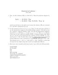
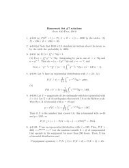
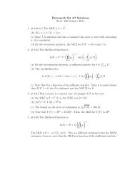
Notes on real numbers
Notes on real numbers

You also want an ePaper? Increase the reach of your titles
YUMPU automatically turns print PDFs into web optimized ePapers that Google loves.
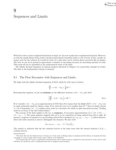
9<br />
Sequences and Limits<br />
This is pag<br />
Printer: Op<br />
With the tools to create complicated functi<strong>on</strong>s in hand, we can now model more complicated situati<strong>on</strong>s. However,<br />
as with the simple Dinner Soup model, solving models almost invariably leads to a lot of work. In fact, usually we<br />
cannot solve for the soluti<strong>on</strong> of a model in terms of a value that can be written down c<strong>on</strong>cretely like an integer.<br />
The best we can do in general is approximate a soluti<strong>on</strong> to increasing accuracy by increasing amounts of work.<br />
This trade-off can be quantified in the mathematical terms of the limit.<br />
The infinite decimal expansi<strong>on</strong> of rati<strong>on</strong>al <strong>numbers</strong> discussed in Chapter 4 is a particular example of a limit.<br />
The limit is the fundamental c<strong>on</strong>cept of analysis. 1<br />
9.1 The First Encounter with Sequences and Limits<br />
We begin with the infinite decimal expansi<strong>on</strong> of 10/9, which by (4.6) can be written<br />
10<br />
9 = 1.11 · · · 11 n + 1 9 10−n .<br />
Rewriting this equati<strong>on</strong>, we get an estimate <strong>on</strong> the difference between 1.111 · · · 11 n and 10/9,<br />
10<br />
∣ 9 − 1.11 · · · 11 n∣ ≤ 10−n . (9.1)<br />
If we c<strong>on</strong>sider 1.11 · · · 11 n as an approximati<strong>on</strong> of 10/9 then (9.1) means that the error |10/9 − 1.11 · · · 11 n | can<br />
be made arbitrarily small by taking n large. If we want the error to be smaller than 10 −9 then we simply choose<br />
n ≥ 10. Computing 1.11 · · · 1 n requires more work as n increases, for which we gain increased accuracy. Trading<br />
work for accuracy is the idea behind limits. 2<br />
The c<strong>on</strong>cept of the limit applies to the set, or sequence, of successive approximati<strong>on</strong>s {1.1, 1.11, 1.111, · · · ,<br />
1.1 · · · 1 n , · · · }. The name sequence suggests that set is to be c<strong>on</strong>sidered as being ordered from left to right. In<br />
general, a sequence of <strong>numbers</strong> is a neverending ordered list of <strong>numbers</strong> {a 1 , a 2 , a 3 , · · · , a n , · · · } called elements,<br />
where the index notati<strong>on</strong> is used to distinguish the elements. We also write<br />
{a 1 , a 2 , a 3 , · · · , a n , · · · } = {a n } ∞ n=1.<br />
The symbol ∞ indicates that the list c<strong>on</strong>tinues forever in the same sense that the natural <strong>numbers</strong> 1, 2, 3, ...,<br />
c<strong>on</strong>tinue forever.<br />
1 The limit also has the dubious h<strong>on</strong>or of being <strong>on</strong>e of the more c<strong>on</strong>fusing topics in analysis and the history of analysis has been<br />
a struggle to come to grips with certain evasive aspects of its definiti<strong>on</strong>.<br />
2 An estimate like (9.1) gives a quantitative measurement of how much accuracy is gained for each increase in work, and so such<br />
estimates are useful not <strong>on</strong>ly to mathematicians but to engineers and scientists.
70 9. Sequences and Limits<br />
Example 9.1. The sequence of even natural <strong>numbers</strong> can be written<br />
{2, 4, 6, · · · } = {2n} ∞ n=1<br />
and the odd natural <strong>numbers</strong> as<br />
and some other sequences:<br />
{1, 3, 5, 7, · · · } = {2n − 1} ∞ n=1<br />
{1, 1 2 2 , 1 3 2 , 1 } { } ∞ 1<br />
4 2 , · · · =<br />
n 2 n=1<br />
{ 1<br />
3 2 , 1 } { } ∞ 1<br />
4 2 , · · · =<br />
n 2 n=3<br />
{1, 2, 4, 8, · · · } = {2 i } ∞ i=0<br />
{−1, 1, −1, 1, −1 · · · } = {(−1) j } ∞ j=1<br />
{1, 1, 1, · · · } = {1} ∞ k=1.<br />
Note the index of a sequence is a dummy variable that can be called anything we like.<br />
Example 9.2.<br />
{<br />
n + n<br />
2 } ∞<br />
n=1 = { j + j 2} ∞<br />
j=1 = { Frodo + (Frodo) 2} ∞<br />
Frodo =1 .<br />
We can also change its value so the sequence begins with a different number by reformulating the coefficients.<br />
Example 9.3.<br />
{<br />
1 + 1 2 , 2 + 2 2 , 3 + 3 2 , · · · } = { n + n 2} ∞<br />
n=1 = { (j − 2) + (j − 2) 2} ∞<br />
j=3 .<br />
See Problems 9.1–9.3.<br />
The sequence {1.11 · · · 11 n } ∞ n=1 has the property that each number in the sequence is a better approximati<strong>on</strong><br />
to 10/9 than the preceding number and as we move from left to right the <strong>numbers</strong> approach 10/9 in value. In<br />
c<strong>on</strong>trast, a single element, even <strong>on</strong>e with many digits like 1.1111111111111, has a fixed accuracy. We say that<br />
the sequence {1.11 · · · 11 n } ∞ n=1 c<strong>on</strong>verges to 10/9 and that 10/9 is the limit of the sequence {1.11 · · · 11 n } ∞ n=1<br />
because the difference between 10/9 and 1.11 · · · 11 n can be made arbitrarily small by taking the index large.<br />
9.2 The Mathematical Definiti<strong>on</strong> of a Limit<br />
The estimate (9.1) implies that 10/9 can be approximated to any specified accuracy by taking terms in the<br />
sequence with sufficiently large index. This is the observati<strong>on</strong> that we use to define the c<strong>on</strong>vergence of a general<br />
sequence. We explain the logic of the definiti<strong>on</strong> with an example.<br />
Example 9.4. To tighten or loosen a hex bolt with head diameter 2/3, a mechanic needs to use a socket<br />
wrench of a slightly bigger size. The tolerance <strong>on</strong> the difference between the sizes of the bolt and the wrench<br />
depend <strong>on</strong> the tightness, the material of the bolt and the wrench, and c<strong>on</strong>diti<strong>on</strong>s such as whether the bolt<br />
threads are lubricated and whether the bolt is rusty or not. If the wrench is too large, then the head of the<br />
bolt is in danger of being stripped before the bolt can be tightened or loosened. Two wrenches with different<br />
tolerances are shown in Fig. 9.1.<br />
Now suppose that we have an infinite set of wrenches of sizes .7, .67, .667, · · · that can be represented as a<br />
sequence {.66 · · · 667 n } ∞ n=1. In every case the wrenches are bigger than 2/3, but not by much. In fact, we ask<br />
you to show that ∣ ∣∣∣<br />
.66 · · · 667 n −<br />
3∣<br />
2 ∣ < 10−n (9.2)<br />
in Problem 9.5. Naturally, (9.2) suggests that the sequence {.6 · · · 67 n } ∞ n=1 c<strong>on</strong>verges to the limit 2/3.<br />
What does this mean in practical terms for the mechanic? Given any specified tolerance <strong>on</strong> the size, she can<br />
reach into the tool chest and pull out a wrench that meets the criteria. The accuracy tolerance is not up<br />
to the mechanic, it is specified by some sec<strong>on</strong>d party like a bicycle manufacturer. Rather, the mechanic has<br />
to meet any specified accuracy to avoid voiding a warranty. The cost of being able to meet any specified<br />
tolerance is having to stock an expensive set of wrenches.
9.2 The Mathematical Definiti<strong>on</strong> of a Limit 71<br />
FIGURE 9.1. Two socket wrenches with different tolerances.<br />
In general, we say that a sequence {a n } ∞ n=1 c<strong>on</strong>verges to a limit A if it is possible to make the terms a n<br />
arbitrarily close to A by taking the index n sufficiently large. In other words, the difference |a n − A| can be made<br />
as small as desired by taking n large. When this is true, we write<br />
lim a n = A.<br />
n→∞<br />
It is c<strong>on</strong>venient to translate this definiti<strong>on</strong> into mathematical notati<strong>on</strong>. From the statement, we can guess that<br />
there are two quantities involved: a bound <strong>on</strong> the size of |a n − A| and a corresp<strong>on</strong>ding number that indicates<br />
how large the index has to be to achieve the bound.<br />
In the two examples c<strong>on</strong>sidered so far, the relati<strong>on</strong> between the size of |a n − A| and n is given by (9.1) and<br />
(9.2), both of which guarantee that a n agrees with A to at least n − 1 decimal places. But in general we cannot<br />
expect to gain a whole digit of accuracy each time n is increased by 1. So the mathematical statement of the<br />
c<strong>on</strong>vergence has to be more flexible. Therefore, we specify the size of |a n − A| by using a general variable ɛ rather<br />
than specifying a number of digits. 3 The bound <strong>on</strong> |a n − A| should be satisfied for all sufficiently large n. In<br />
other words, given ɛ, there should be a number N such that the bound is satisfied for all n larger than N. 4<br />
Putting this together, the mathematical statement that a sequence c<strong>on</strong>verges to a limit reads<br />
if for any ɛ > 0 there is a number N > 0 such that<br />
lim a n = A<br />
n→∞<br />
|a n − A| ≤ ɛ for all n ≥ N.<br />
We emphasize that the value of N depends <strong>on</strong> ɛ, and in particular, we expect that decreasing ɛ means that N<br />
increases.<br />
Example 9.5. We verify the definiti<strong>on</strong> for {1.11 · · · 11 n } ∞ n=1. We want to show 5 that given ɛ > 0 there is a<br />
N > 0 such that ∣ ∣∣∣<br />
1.11 · · · 11 n − 10 9 ∣ ≤ ɛ<br />
for all n ≥ N. Suppose that ɛ has the decimal expansi<strong>on</strong><br />
ɛ = 0.000 · · · 00p m p m+1 · · ·<br />
where the first digit of ɛ that is n<strong>on</strong>zero is p m in the mth place. By (9.1), if we choose n ≥ m, then<br />
∣ 1.11 · · · 11 n − 10 9 ∣ ≤ 10−n = .00 · · · 001 ≤ ɛ.<br />
Therefore given any ɛ > 0, if we choose N = m where the first n<strong>on</strong>zero digit of ɛ is in the mth place, then<br />
|1.11 · · · 11 n − 10/9| < ɛ for n ≥ N.<br />
We next present a couple of less familiar examples.<br />
3 Traditi<strong>on</strong>ally, ɛ and δ are used to denote small quantities, though not interchangeably. Thinking of δ as “difference” and ɛ as<br />
“error” may help clarify their usage.<br />
4 What happens if the bound is satisfied for <strong>on</strong>ly some of the n larger than N? We address this questi<strong>on</strong> in Chapter 32.<br />
5 It is often helpful to begin these problems by writing out the definiti<strong>on</strong>.
72 9. Sequences and Limits<br />
Example 9.6. We show that {1/n} ∞ n=1 c<strong>on</strong>verges to 0, i.e.,<br />
1<br />
lim<br />
n→∞ n = 0.<br />
This is intuitively obvious since 1/n can be made as close to 0 as desired by taking n large. It is also visible in<br />
a plot of the elements of the sequence (see Fig. 5.5). But to satisfy the annoying mathematician who specifies<br />
an ɛ > 0, we show there is an N > 0 such that<br />
∣ 1 ∣∣∣<br />
∣n − 0 ≤ ɛ<br />
for all n ≥ N. In this case, it is not too hard to determine N since n ≥ 1/ɛ implies that 1/n ≤ ɛ. Therefore<br />
given any ɛ > 0, if N = 1/ɛ then<br />
∣ 1 ∣∣∣<br />
∣n − 0 = 1 n ≤ ɛ (9.3)<br />
for n ≥ N. Note that if ɛ decreases then N naturally increases.<br />
In Problem 9.8, we ask you to show that<br />
where p is any natural number.<br />
Example 9.7. We show that<br />
lim<br />
n→∞<br />
lim<br />
n→∞<br />
1<br />
n p = 0<br />
1<br />
2 n = 0.<br />
This limit is suggested by c<strong>on</strong>sidering a plot of the elements of the sequence (see Fig. 5.5). By the definiti<strong>on</strong>,<br />
given ɛ > 0, we show that there is an N such that<br />
∣ 1 ∣∣∣<br />
∣2 n − 0 = 1<br />
2 n ≤ ɛ<br />
for n ≥ N. Certainly<br />
so given any natural number m<br />
2 4 = 16 ≥ 10<br />
1<br />
2 4m ≤ 1<br />
10 m .<br />
So if ɛ has the decimal expansi<strong>on</strong> ɛ = 0.000 · · · 00p m p m+1 · · · , where the first digit of ɛ that is n<strong>on</strong>zero is p m<br />
in the mth place, then<br />
1<br />
2 4m ≤ 1<br />
10 m ≤ ɛ.<br />
Therefore, given any ɛ > 0, if N = 4m, where the first n<strong>on</strong>zero digit of ɛ is in the mth place, then |1/2 n −0| < ɛ<br />
for n ≥ N.<br />
In general, it is possible to show that<br />
lim<br />
n→∞ rn = 0<br />
when |r| < 1 by using a proof similar to the case r = 1/2. We ask you to do the case |r| < 1/2 in Problem 9.9.<br />
We can show the general result easily after introducing the logarithm in Chapter 28.<br />
We c<strong>on</strong>tinue with a more complicated example.<br />
Example 9.8. We show that the limit of the sequence { n<br />
n+1 }∞ n=1 = { 1 2 , 2 3<br />
, · · · } equals 1, that is<br />
lim<br />
n→∞<br />
n<br />
= 1. (9.4)<br />
n + 1<br />
This is suggested by a plot of the elements (see Fig. 9.2). We begin by simplifying the difference<br />
∣ 1 − n<br />
∣ ∣∣∣ n + 1∣ = n + 1 − n<br />
n + 1 ∣ = 1<br />
n + 1 .
9.3 Some Background <strong>on</strong> the Definiti<strong>on</strong> of a Limit 73<br />
1.0<br />
0.5<br />
0.0<br />
0 10 20 30<br />
n<br />
FIGURE 9.2. The elements of the sequence {n/(n + 1)}.<br />
n<br />
Note that this intuitively shows that<br />
n+1<br />
can be made arbitrarily close to 1 by taking n large and so 1 is the<br />
limit. To verify the definiti<strong>on</strong>, suppose ɛ > 0 is given. By the equality above,<br />
∣ 1 − n<br />
n + 1∣ = 1<br />
n + 1 ≤ ɛ<br />
provided that n ≥ 1/ɛ − 1. Given ɛ > 0, if N ≥ 1/ɛ − 1, then<br />
for n ≥ N.<br />
∣ 1 − n<br />
n + 1∣ ≤ ɛ<br />
We c<strong>on</strong>clude with an important observati<strong>on</strong>. The examples of c<strong>on</strong>vergent sequences presented so far have the<br />
property that the elements of the sequence are rati<strong>on</strong>al and the limit of the sequence is a rati<strong>on</strong>al number. This<br />
is important because up to now arithmetic is <strong>on</strong>ly defined for rati<strong>on</strong>al <strong>numbers</strong>, and subtracti<strong>on</strong> is used in the<br />
definiti<strong>on</strong> of the limit. In other words, the definiti<strong>on</strong> of a limit presented so far <strong>on</strong>ly makes sense if the sequence<br />
c<strong>on</strong>sists of rati<strong>on</strong>al <strong>numbers</strong> and the limit of the sequence is a rati<strong>on</strong>al number.<br />
This raises the questi<strong>on</strong>: does a c<strong>on</strong>vergent sequence of rati<strong>on</strong>al <strong>numbers</strong> always c<strong>on</strong>verge to a rati<strong>on</strong>al number?<br />
The short answer is no, and therein lies a mystery that c<strong>on</strong>founded generati<strong>on</strong>s of mathematicians attempting to<br />
establish a rigorous foundati<strong>on</strong> for analysis. We explain how this can be in Chapter 10. In this chapter, we simply<br />
assume that all sequences c<strong>on</strong>sist of rati<strong>on</strong>al <strong>numbers</strong>, all c<strong>on</strong>vergent sequences c<strong>on</strong>verge to a rati<strong>on</strong>al limit, and<br />
the domains and ranges of all functi<strong>on</strong>s are c<strong>on</strong>tained in Q. Technically, this means that the discussi<strong>on</strong> in this<br />
chapter does not apply to all rati<strong>on</strong>al sequences that c<strong>on</strong>verge. In Chapter 11, we show that this assumpti<strong>on</strong> can<br />
be removed and the results in this chapter do hold for general sequences of <strong>numbers</strong>.<br />
9.3 Some Background <strong>on</strong> the Definiti<strong>on</strong> of a Limit<br />
Leibniz and Newt<strong>on</strong> 6 implicitly used the idea of limits in their versi<strong>on</strong>s of calculus. Newt<strong>on</strong> in particular formulated<br />
a definiti<strong>on</strong> in words that is close to the modern definiti<strong>on</strong>. But they did not express the idea of a<br />
limit in quantitative terms, and this opened up the early versi<strong>on</strong>s of calculus to criticism about its rigor. As a<br />
c<strong>on</strong>sequence, there was increasing recogniti<strong>on</strong> of the need for a more precise definiti<strong>on</strong> of a limit am<strong>on</strong>g mathematicians<br />
following Leibniz and Newt<strong>on</strong>. Cauchy 7 was the first pers<strong>on</strong> to write down the modern definiti<strong>on</strong> of<br />
6 The English mathematician Sir Isaac Newt<strong>on</strong> (1643–1727) is credited jointly with the discovery of calculus together with<br />
Leibniz. The scope of Newt<strong>on</strong>’s achievements in mathematics and physics has likely never been surpassed by any other individual.<br />
Remarkably, he made some of his most important scientific discoveries, including the compositi<strong>on</strong> of white light, calculus, and his<br />
law of gravitati<strong>on</strong>, while waiting out the Great Plague of 1644–45 at home. A few years later, Newt<strong>on</strong> became the Lucasian Professor<br />
at Cambridge University; a positi<strong>on</strong> he held for eighteen productive years. Though active in scientific politics, Newt<strong>on</strong> tended to<br />
publish his results many years after they were derived, and <strong>on</strong>ly then at the urging of his colleagues. Newt<strong>on</strong> was always pr<strong>on</strong>e to<br />
depressi<strong>on</strong> and nervous irritability and the strain of publishing his renowned Principia caused him to turn away from research in<br />
physics and mathematics for the last forty years of his life. During this period, Newt<strong>on</strong> worked successfully as Master of the Mint<br />
and acquired a fortune. He also worked in theology and alchemy, producing little that is remembered.<br />
7 Augustin Louis Cauchy (1789–1857) was born and worked in France. Cauchy was incredibly productive, publishing nearly as<br />
many papers as Euler (789) while producing fundamentally important results in nearly all areas of mathematics including <strong>real</strong> and<br />
complex analysis, ordinary and partial differential equati<strong>on</strong>s, matrix theory, Fourier theory, elasticity, and the theory of light. Cauchy<br />
worried about the foundati<strong>on</strong>s of analysis and gave the first rigorous proofs of some well-known results in calculus, including the first<br />
general existence result for ordinary differential equati<strong>on</strong>s and the Mean Value Theorem. Cauchy wrote down the first “ɛ-δ proof” in<br />
proving the Mean Value Theorem. Cauchy was a principled pers<strong>on</strong> in political terms and his career path took up and down swings<br />
as the political winds changed.
74 9. Sequences and Limits<br />
the limit. We owe the notati<strong>on</strong> “lim” to Weierstrass, 8 who was also a key figure in clarifying the mathematical<br />
meaning of the limit.<br />
9.4 Divergent Sequences<br />
For the sake of comparis<strong>on</strong>, it is a good idea to examine some sequences that do not c<strong>on</strong>verge, or diverge. There<br />
are lots of ways for a sequence to diverge; for example, c<strong>on</strong>sider the divergent sequences<br />
{−6, 2, −.4, −.7, 5, 6.1, 2, 9.9, −3, .2, 1, 7, 28, .3, −5.4, · · · }, (9.5)<br />
{(−1) n } ∞ n=1 = {−1, 1, −1, 1, · · · }, (9.6)<br />
{(−n) n } ∞ n=1 = {−1, 4, −27, · · · }, (9.7)<br />
{n 2 } ∞ n=1 = {1, 4, 9, 16, · · · }. (9.8)<br />
In each case, there is no single number that the terms in the sequence approach as n increases. In general, we<br />
expect that if the elements of a sequence are written down at “random” it is likely that the sequence diverges.<br />
The sequences that c<strong>on</strong>verge are special.<br />
Also in general, there is relatively little that can be said about a divergent sequence. However, we do distinguish<br />
<strong>on</strong>e special case of divergence. No pattern in the elements of (9.5) can be seen, while the elements of (9.6) oscillate<br />
between two values, but never get close to <strong>on</strong>e value. The elements of (9.7) also oscillate, but now become bigger<br />
as the index increases. Whereas the elements of (9.8) simply become bigger as the index increases, which is<br />
predictable behavior. We distinguish this case by saying that a sequence diverges to infinity, and write<br />
lim a n = ∞,<br />
n→∞<br />
whenever the terms grow without bound as the index increases. Mathematically, we say that a sequence diverges<br />
to infinity if given any positive M there is a natural number N such that a n ≥ M for n ≥ N.<br />
Example 9.9. We show that lim n→∞ n 2 = ∞ by verifying the definiti<strong>on</strong>. For n ≥ 1, n 2 ≥ n. Hence, given<br />
any M<br />
n 2 ≥ n ≥ M,<br />
provided n ≥ M. This means we take N = M.<br />
Similarly, we say that the sequence diverges to minus infinity, and write<br />
lim a n = −∞,<br />
n→∞<br />
if given any negative M we can find a natural number N such that a n ≤ M for n ≥ N.<br />
9.5 Infinite Series<br />
An important example of sequences is provided by series, or infinite sums. We begin by recalling the geometric<br />
sum discussed in Chapter 3.<br />
Example 9.10. Recall that the sum<br />
1 + r + r 2 + · · · + r n =<br />
n∑<br />
i=0<br />
r i<br />
8 Karl Theodor Wilhelm Weierstrass (1815–1897) began his career as a high school teacher before bursting <strong>on</strong> the mathematical<br />
scene with a few papers and acquiring a professorship at the University of Berlin. Weierstrass made fundamental c<strong>on</strong>tributi<strong>on</strong>s to<br />
bilinear forms, infinite series and products, the theory of functi<strong>on</strong>s, the calculus of variati<strong>on</strong>s, and the foundati<strong>on</strong>s of <strong>real</strong> analysis.<br />
While Weierstrass published relatively few papers, he was a tremendous lecturer, and his seminars and courses had great impact<br />
<strong>on</strong> mathematics. Much of the modern c<strong>on</strong>cern with complete rigor in analysis originated with Weierstrass. Weierstrass introduced<br />
the notati<strong>on</strong> lim, | |, and the ɛ-δ definiti<strong>on</strong>s of c<strong>on</strong>tinuity and limit of a functi<strong>on</strong>. Weierstrass was also the first mathematician to<br />
sp<strong>on</strong>sor a woman for a doctorate degree. This was the talented Russian mathematician Sofia Vasilyevna Kovalevskaya (1850–1891).
9.5 Infinite Series 75<br />
is called the geometric sum of order n with factor r. Both to understand infinite decimal expansi<strong>on</strong>s and<br />
the Verhulst populati<strong>on</strong> model in Secti<strong>on</strong> 4.4, we determined the value of this sum as we take more and more<br />
terms. If we let<br />
n∑<br />
s n = r i ,<br />
then this is the same thing as studying the c<strong>on</strong>vergence of the sequence {s n } ∞ n=0.<br />
To study the c<strong>on</strong>vergence, we use the formula<br />
s n =<br />
n∑<br />
i=0<br />
i=0<br />
r i = 1 − rn+1<br />
1 − r<br />
that was proved using inducti<strong>on</strong> for any r ≠ 1. If |r| < 1, then as n increases r n+1 approaches zero in value.<br />
Hence it is reas<strong>on</strong>able to guess that<br />
lim s n = 1<br />
n→∞ 1 − r<br />
for |r| < 1. This is also suggested by plotting s n , as in Fig. 9.3.<br />
1.0<br />
s n<br />
0.5<br />
0.0<br />
0 10 20 30<br />
n<br />
FIGURE 9.3. The elements of the partial sum {s n} of the geometric series with r = −.9.<br />
We verify this is true using the definiti<strong>on</strong> of the limit. Given ɛ > 0, we show there is an N such that<br />
1 − r n+1<br />
∣ − 1<br />
∣ ∣∣∣ 1 − r 1 − r ∣ = r n+1<br />
1 − r ∣ ≤ ɛ<br />
for all n ≥ N. Equivalently, given ɛ > 0 we show there is an N > 0 such that<br />
|r| n+1 ≤ ɛ |1 − r| (9.9)<br />
for |r| < 1. But ɛ|1 − r| is a fixed number <strong>on</strong>ce ɛ is specified, while |r| N+1 can be made as small as desired<br />
by taking N sufficiently large when |r| < 1. Certainly (9.9) holds for any n ≥ N <strong>on</strong>ce N is determined. This<br />
verifies the definiti<strong>on</strong> of c<strong>on</strong>vergence, albeit rather vaguely. After we introduce the logarithm in Chapter 28,<br />
an exact relati<strong>on</strong>ship between N and ɛ is easy to determine.<br />
Based <strong>on</strong> this result, we call the limit of {s n } ∞ n=0 the geometric series and write<br />
lim s n =<br />
n→∞<br />
∞∑<br />
r i = 1 + r + r 2 + · · · .<br />
i=0<br />
Since this limit is defined for |r| < 1, we say the geometric series c<strong>on</strong>verges for |r| < 1 and write<br />
1 + r + r 2 + · · · = 1<br />
1 − r . (9.10)<br />
The sequence {s n } ∞ n=0 is called the sequence of partial sums of the series.<br />
In general, the infinite series<br />
∞∑<br />
a i = a 0 + a 1 + · · ·<br />
i=0
76 9. Sequences and Limits<br />
is defined to be the limit of the sequence {s n } ∞ n=0 of partial sums<br />
s n =<br />
when the limit is defined. In this case, we say the infinite series c<strong>on</strong>verges.<br />
If the sequence of partial sums of a series diverges to infinity or minus infinity, then we say that the series<br />
diverges to infinity or minus infinity.<br />
n∑<br />
i=0<br />
Example 9.11. The series ∑ ∞<br />
i=1<br />
i = 1 + 2 + 3 + · · · diverges to infinity. This follows because the partial<br />
sum s n = ∑ n<br />
i=1 i satisfies s n ≥ n for all n. Therefore the partial sums increase without bound as the index<br />
increases.<br />
In this book, infinite series are given much less space than is usual for calculus and analysis texts. Historically,<br />
infinite series were crucial to the development of analysis. Indeed, much of early analysis, including differentiati<strong>on</strong><br />
formulas, integrati<strong>on</strong>, and the existence of soluti<strong>on</strong>s of differential equati<strong>on</strong>s, was justified using the properties<br />
of infinite series, and many important analysts worked <strong>on</strong> the properties of infinite series. Nevertheless, the role<br />
of infinite series in <strong>real</strong> analysis, which is analysis in the space of <strong>real</strong> <strong>numbers</strong>, has diminished greatly in this<br />
century. 9<br />
There is a fundamental difference between the smoothness of functi<strong>on</strong>s encountered in <strong>real</strong> analysis and those<br />
encountered in complex analysis, which is analysis in the space of complex <strong>numbers</strong>. The so-called analytic<br />
functi<strong>on</strong>s that lie at the heart of complex analysis are very smooth and for this reas<strong>on</strong> are closely c<strong>on</strong>nected to<br />
infinite series. 10 For this reas<strong>on</strong>, infinite series remain a central topic of complex analysis. We believe the natural<br />
place to learn about infinite series is in a course in complex analysis, and point to Ahlfors [1], for example.<br />
a i<br />
9.6 Limits are Unique<br />
In the next few secti<strong>on</strong>s, we work out some useful properties of c<strong>on</strong>vergent sequences. The sequences studied in this<br />
book are usually c<strong>on</strong>structed as approximati<strong>on</strong>s to some quantity that we want to compute, e.g., {1.11 · · · 1 n } ∞ n=1<br />
is a sequence of approximati<strong>on</strong>s to 10/9. The properties developed in this chapter make it possible to combine<br />
approximati<strong>on</strong>s of different quantities to form an approximati<strong>on</strong> of a new quantity.<br />
We begin with the observati<strong>on</strong> that the limit of a c<strong>on</strong>vergent sequence is unique. It certainly makes sense that<br />
it is impossible for the terms in a sequence to become arbitrarily close to two different <strong>numbers</strong> at the same<br />
time. Suppose in fact that a sequence {a n } ∞ n=1 c<strong>on</strong>verges to two <strong>numbers</strong> A and B. To show that A and B are<br />
equal, we show that the distance |A − B| is zero. To estimate this difference, we use a variati<strong>on</strong> of the triangle<br />
inequality (2.4) that reads<br />
|a − b| ≤ |a − c| + |c − b| for all a, b, c. (9.11)<br />
We ask you to prove this in Problem 9.14. Using (9.11) with a = A, b = B, and c = a n , we get<br />
|A − B| ≤ |a n − A| + |a n − B|<br />
for any n. Now because a n c<strong>on</strong>verges to A, both |a n − A| and |a n − B| can be made smaller than |A − B|/4 by<br />
taking n sufficiently large. But this means that |A − B| ≤ |A − B|/2, which can <strong>on</strong>ly hold if |A − B| = 0.<br />
Theorem 9.1 A sequence can have at most <strong>on</strong>e limit.<br />
On this topic, there is a minor hiccup regarding the uniqueness of infinite decimal expansi<strong>on</strong>s. For example,<br />
it is straightforward to show (Problem 9.15) that lim n→∞ 0.99 · · · 99 n = 1. This means that 1 has two decimal<br />
representati<strong>on</strong>s, namely, 1.000 · · · = 0.9999 · · · . So we have to decide what we mean when we write a = b, where<br />
a and b are not written in the same way.<br />
A standard approach is to interpret a = b as meaning that we can show that |a − b| is smaller than any<br />
positive number. This is equivalent to writing a = 0 if we can show that |a| is smaller than any positive number.<br />
Corresp<strong>on</strong>dingly if |a| is bigger than some positive number then we write a ≠ 0. With this definiti<strong>on</strong>, we can<br />
write .999 · · · = 1 without trouble. 11 Another approach is to simply avoid decimal representati<strong>on</strong>s ending in<br />
9 This is <strong>on</strong>e reas<strong>on</strong> that the chapter <strong>on</strong> infinite series in a standard calculus book is <strong>on</strong>e of the least popular and least motivated<br />
topics from the students’ point of view.<br />
10 The c<strong>on</strong>necti<strong>on</strong> between smoothness of functi<strong>on</strong>s and infinite series is discussed further in Chapter 37.<br />
11 However, this interpretati<strong>on</strong> could trouble a c<strong>on</strong>structivist because verifying that a = b for arbitrary a and b nominally requires<br />
showing |a − b| is smaller than an infinite number of positive <strong>numbers</strong>. Verifying that |a − b| is smaller than any finite number of<br />
positive <strong>numbers</strong> can not settle the issue. This is discussed in more detail in Chapter 11.
9.7 Arithmetic with Sequences 77<br />
repeated digits of 9 by replacing any such expansi<strong>on</strong> by the equivalent expansi<strong>on</strong> ending with all 0 digits. Hence<br />
when .999 · · · occurs, it is replaced by 1.000 · · · = 1.<br />
9.7 Arithmetic with Sequences<br />
It turns out that if we perform arithmetic <strong>on</strong> sequences that c<strong>on</strong>verge, we end up with another c<strong>on</strong>vergent<br />
sequence. For example, suppose that {a n } ∞ n=1 c<strong>on</strong>verges to A and {b n } ∞ n=1 c<strong>on</strong>verges to B. Then {a n + b n } ∞ n=1,<br />
the sequence obtained by adding the terms of each individual sequence, c<strong>on</strong>verges to A + B. Since we are trying<br />
to prove that {a n + b n } ∞ n=1 c<strong>on</strong>verges to A + B, we estimate the difference |(a n + b n ) − (A + B)|. Inequality (9.11)<br />
implies<br />
|(a n + b n ) − (A + B)| = |(a n − A) + (b n − B)|<br />
≤ |a n − A| + |b n − B|.<br />
Since |a n − A| and |b n − B| can be made as small as desired by taking n large, |(a n + b n ) − (A + B)| can be made<br />
as small as desired by taking n large. 12<br />
Likewise, {a n b n } ∞ n=1 c<strong>on</strong>verges to AB. This requires a frequently useful trick of adding and subtracting the<br />
same quantity. We have<br />
|(a n b n ) − (AB)| = |a n b n − a n B + a n B − AB|<br />
= |a n (b n − B) + B(a n − A)|<br />
≤ |a n ||b n − B| + |B||a n − A|.<br />
We also need the fact that the <strong>numbers</strong> |a n | are smaller than |A| + 1 for n large, which follows because |a n − A|<br />
can be made as small as desired for n large. So for n large,<br />
|(a n b n ) − (AB)| ≤ (|A| + 1)|b n − B| + |B||a n − A|.<br />
Now we can make the differences <strong>on</strong> the right arbitrarily small by taking n large.<br />
The analogous properties hold for the difference and quotient of two sequences (Problems 9.16 and 9.18). We<br />
summarize as a theorem.<br />
Theorem 9.2 Suppose that {a n } ∞ n=1 c<strong>on</strong>verges to A and {b n } ∞ n=1 c<strong>on</strong>verges to B. Then {a n + b n } ∞ n=1 c<strong>on</strong>verges<br />
to A + B, {a n − b n } ∞ n=1 c<strong>on</strong>verges to A − B, {a n b n } ∞ n=1 c<strong>on</strong>verges to AB, and if b n ≠ 0 for all n and B ≠ 0,<br />
{a n /b n } ∞ n=1 c<strong>on</strong>verges to A/B.<br />
We say that a sequence {a n } is bounded if there is a c<strong>on</strong>stant M such that |a n | ≤ M for all indices n. The<br />
previous argument also justifies the following theorem We ask you to provide the details in Problem 9.27.<br />
Theorem 9.3 A c<strong>on</strong>vergent sequence is bounded.<br />
This discussi<strong>on</strong> is a bit tedious but it can make computing the limit of a complicated sequence much easier.<br />
Example 9.12. C<strong>on</strong>sider {2 + 3n −4 + (−1) n n −1 } ∞ n=1.<br />
lim (2 +<br />
n→∞ 3n−4 + (−1) n n −1 ) = lim 2 + 3 lim<br />
n→∞ n→∞ n−4 + lim<br />
n→∞ (−1)n n −4<br />
= 2 + 3 × 0 + 0 = 2.<br />
Example 9.13. We compute the limit of<br />
{4 1 + n−3<br />
3 + n −2 } ∞<br />
n=1<br />
12 This proof introduces a new level of sophisticati<strong>on</strong> into discussi<strong>on</strong>s involving c<strong>on</strong>vergence. We did not write down the formal<br />
definiti<strong>on</strong> of c<strong>on</strong>vergence to a limit with its ɛ and corresp<strong>on</strong>ding N. Rather, we use informal language about making certain quantities<br />
“as small as desired” by choosing indices “sufficiently large.” Once we understand how to argue from the formal definiti<strong>on</strong>, then it<br />
is c<strong>on</strong>venient to use informal language. But we point out that we can modify this and the following informal arguments to use the<br />
definiti<strong>on</strong> of c<strong>on</strong>vergence. We pose this as Problem 9.19.
78 9. Sequences and Limits<br />
by using Theorem 9.2 to argue<br />
lim 4 1 + n−3<br />
= lim<br />
n→∞ 3 + n−2 4 lim ( )<br />
n→∞ 1 + n<br />
−3<br />
(<br />
n→∞ lim )<br />
n→∞ 3 + n<br />
−2<br />
= 4 lim n→∞ 1 + lim n→∞ n −3<br />
lim n→∞ 3 + lim n→∞ n −2<br />
= 4 1 + 0<br />
3 + 0 = 4 3 .<br />
Each step in the computati<strong>on</strong>s in Examples 9.12 and 9.13 is justified because we obtain new limits that<br />
are defined after every applicati<strong>on</strong> of Theorem 9.2. On the other hand, if we attempt to use Theorem 9.2 to<br />
manipulate a sequence and end up with limits that are undefined at some point, then the computati<strong>on</strong> is not<br />
justified by Theorem 9.2.<br />
Example 9.14. We cannot directly apply Theorem 9.2 to compute<br />
( 1<br />
lim<br />
n→∞ n − 1 )<br />
.<br />
n + 1<br />
If we try, we obtain<br />
( 1<br />
lim<br />
n→∞ n − 1 )<br />
1<br />
“ = ” lim<br />
n + 1<br />
n→∞ n − lim 1<br />
n→∞ n + 1 ,<br />
and neither of the two limits <strong>on</strong> the right are defined. To compute this limit, we first find a comm<strong>on</strong> denominator<br />
1<br />
n − 1<br />
n + 1 = n + 1 − n<br />
n(n + 1) = 1<br />
n(n + 1) .<br />
Clearly, then we have<br />
( 1<br />
lim<br />
n→∞ n − 1 )<br />
1<br />
= lim<br />
n + 1 n→∞ n(n + 1) = 0.<br />
9.8 Functi<strong>on</strong>s and Sequences<br />
A comm<strong>on</strong> way to make a complicated sequence is to apply a functi<strong>on</strong> to each term in a sequence and there by<br />
get a new sequence.<br />
Example 9.15. In the Verhulst model Model 4.4, we c<strong>on</strong>sider the sequence<br />
⎧<br />
⎫∞<br />
⎪⎨<br />
{P n } ∞ 1<br />
⎪⎬<br />
n=1 =<br />
1 ⎪⎩<br />
2 n Q 0 + 1 (<br />
1 − 1 ) .<br />
⎪⎭<br />
K 2 n<br />
The sequence {P n } is obtained by applying the functi<strong>on</strong><br />
to the terms in the sequence { 1<br />
2 n }<br />
.<br />
1<br />
f(x) =<br />
Q 0 x + 1 K<br />
(1 − x)<br />
Example 9.16. As part of solving the Muddy Yard model in Chapter 10, we need to compute<br />
( ) 2<br />
lim an<br />
n→∞<br />
for a special sequence {a n } . Here, we have applied f(x) = x 2 to {a n }.<br />
Therefore, it is natural to investigate the c<strong>on</strong>vergence of a sequence obtained by applying a functi<strong>on</strong> to a<br />
c<strong>on</strong>vergent sequence.<br />
By the way, there are usually several different ways to write a given sequence in terms of functi<strong>on</strong>s and other<br />
sequences.<br />
n=1
Example 9.17. C<strong>on</strong>sider<br />
We can choose {a n } = { 1<br />
n}<br />
and f(x) = (x 2 + 3) 4 so (9.12) can be written<br />
lim f(a (<br />
n) = lim (an ) 2 + 3 ) 4<br />
.<br />
n→∞ n→∞<br />
9.8 Functi<strong>on</strong>s and Sequences 79<br />
lim<br />
(<br />
n −2 + 3 ) 4<br />
. (9.12)<br />
n→∞<br />
We can also choose {a n } = { 1<br />
n 2 }<br />
and f(x) = (x + 3) 4 so (9.12) can be written<br />
lim f(a n) = lim (a n + 3) 4 .<br />
n→∞ n→∞<br />
Another possibility is {a n } = { 1<br />
n<br />
+ 3 } and f(x) = x 4 so (9.12) can be written<br />
2<br />
See Problem 9.4 for more examples.<br />
lim f(a n) = lim (a n) 4 .<br />
n→∞ n→∞<br />
The idea behind c<strong>on</strong>vergence is to show that the terms in a sequence become close to the limit as the index<br />
increases. If we apply a functi<strong>on</strong> to a sequence with a limit and the functi<strong>on</strong> changes arbitrarily with small<br />
changes of input, i.e., the functi<strong>on</strong> is not c<strong>on</strong>tinuous, then we cannot <strong>real</strong>ly expect much.<br />
Example 9.18. The sequence {<br />
−1, 1 2 , −1<br />
3 , 1 } { } (−1)<br />
n<br />
4 , · · · =<br />
n<br />
has the limit<br />
{ } (−1)<br />
n<br />
lim<br />
= 0.<br />
n→∞ n<br />
But the sequence obtained by applying the step functi<strong>on</strong> I(t) to this sequence,<br />
{ ( ( ) ( }<br />
1 −1 1<br />
I(−1), I , I , I , · · · = {0, 1, 0, 1, · · · },<br />
2)<br />
3 4)<br />
diverges.<br />
In other words, it <strong>on</strong>ly makes sense to try to compute the limit in such situati<strong>on</strong>s if the functi<strong>on</strong> behaves<br />
c<strong>on</strong>tinuously. So we assume that the functi<strong>on</strong> is Lipschitz c<strong>on</strong>tinuous.<br />
Now suppose that {a n } c<strong>on</strong>verges to the limit A, where all the a n and A bel<strong>on</strong>g to a set I <strong>on</strong> which f is<br />
Lipschitz c<strong>on</strong>tinuous with Lipschitz c<strong>on</strong>stant L. We define the sequence {b n } by b n = f(a n ) and we show that<br />
lim b n = f(A).<br />
n→∞<br />
Actually this follows directly from the definiti<strong>on</strong>s of a limit and Lipschitz c<strong>on</strong>tinuity. We want to show that<br />
|b n − f(A)| can be made arbitrarily small by taking n large. But<br />
|b n − f(A)| = |f(a n ) − f(A)| ≤ L|a n − A|,<br />
since a n and A are in I. We can make the right-hand side arbitrarily small by taking n sufficiently large since<br />
a n c<strong>on</strong>verges to A. We summarize as<br />
Theorem 9.4 Let {a n } be a sequence with lim n→∞ a n = A and f a Lipschitz c<strong>on</strong>tinuous functi<strong>on</strong> <strong>on</strong> a set I<br />
such that a n is in I for all n and A is in I. Then<br />
( )<br />
lim f(a n) = f lim a n . (9.13)<br />
n→∞ n→∞<br />
Example 9.19. In the Verhulst model Model 4.4, we need to compute<br />
lim P n = lim<br />
n→∞ n→∞<br />
The sequence {P n } is obtained by applying the functi<strong>on</strong><br />
1<br />
1<br />
2 n Q 0 + 1 K<br />
1<br />
f(x) =<br />
Q 0 x + 1 K<br />
(1 − x)<br />
(<br />
1 − 1<br />
2 n ).<br />
to the terms in the sequence { 1<br />
2 n }<br />
. In this case, f is Lipschitz c<strong>on</strong>tinuous <strong>on</strong> any bounded interval, say, [0, 1].<br />
Since 1/2 n is in [0, 1] for all n as is lim n→∞ 1/2 n = 0, we compute easily lim n→∞ P n = f(0) = K.
80 9. Sequences and Limits<br />
Example 9.20. The functi<strong>on</strong> f(x) = x 2 is Lipschitz c<strong>on</strong>tinuous <strong>on</strong> bounded intervals, therefore, if {a n }<br />
c<strong>on</strong>verges to A, then<br />
( ) 2<br />
lim an = A<br />
2<br />
n→∞<br />
We can apply this rule to compute more complicated examples as well.<br />
Example 9.21. By Corollary 8.2 and Theorem 9.2,<br />
( 3 +<br />
1<br />
)9 (<br />
n<br />
3 + 1 )9<br />
n<br />
lim<br />
n→∞ 4 + 2 = lim<br />
n→∞<br />
n<br />
4 + 2 n<br />
(<br />
limn→∞ (3 + 1 n<br />
=<br />
)<br />
)9<br />
lim n→∞ (4 + 2 n<br />
( ) ) 9 3<br />
= .<br />
4<br />
Example 9.22. By Corollary 8.2 and Theorem 9.2,<br />
(<br />
(2 −n ) 7 + 14(2 −n ) 4 − 3(2 −n ) + 2 ) = 2 × 0 7 + 14 × 0 4 − 3 × 0 + 2 = 2.<br />
lim<br />
n→∞<br />
9.9 Sequences with Rati<strong>on</strong>al Elements<br />
We c<strong>on</strong>clude the discussi<strong>on</strong> of computing limits of sequences by c<strong>on</strong>sidering sequences in which the elements<br />
are rati<strong>on</strong>al functi<strong>on</strong>s of the index. Such examples are comm<strong>on</strong> in modeling, and moreover there is a trick that<br />
enables such sequences to be analyzed relatively easily.<br />
Example 9.23. C<strong>on</strong>sider {<br />
6n 2 ∞<br />
+ 2<br />
4n 2 .<br />
− n + 1000}<br />
n=1<br />
Before computing the limit, we work out what happens when n becomes large. In the numerator, 6n 2 is much<br />
larger than 2 when n is large and likewise in the denominator, 4n 2 becomes much larger than −n + 1000 in<br />
size when n is large. So we might guess that for n large,<br />
6n 2 + 2<br />
4n 2 − n + 1000 ≈ 6n2<br />
4n 2 = 6 4 .<br />
To see this is a good guess for the limit, we use a trick to put the sequence in a better form to compute the<br />
limit,<br />
6n 2 + 2<br />
lim<br />
n→∞ 4n 2 − n + 1000 = lim (6n 2 + 2)n −2<br />
n→∞ (4n 2 − n + 1000)n −2<br />
where we finish the computati<strong>on</strong> as usual.<br />
6 + 2n −2<br />
= lim<br />
n→∞ 4 − n −1 + 1000n −2<br />
= 6 4 ,<br />
The trick of multiplying top and bottom of a ratio by a power can also be used to figure out when a sequence<br />
c<strong>on</strong>verges to zero or diverges to infinity.<br />
Example 9.24.<br />
n 3 − 20n 2 + 1 (n 3 − 20n 2 + 1)n −3<br />
lim<br />
n→∞ n 8 = lim<br />
+ 2n n→∞ (n 8 + 2n)n −3<br />
1 − 20n −1 + n −3<br />
= lim<br />
n→∞ n 5 + 2n −2 .<br />
We c<strong>on</strong>clude that the numerator c<strong>on</strong>verges to 1 while the denominator increases without bound. Therefore,<br />
n 3 − 20n 2 + 1<br />
lim<br />
n→∞ n 8 = 0.<br />
+ 2n
Example 9.25.<br />
−n 6 + n + 10 (−n 6 + n + 10)n −4<br />
lim<br />
n→∞ 80n 4 = lim<br />
+ 7 n→∞ (80n 4 + 7)n −4<br />
−n 2 + n −3 + 10n −4<br />
= lim<br />
n→∞ 80 + 7n −4 .<br />
9.10 Calculus and Computing Limits 81<br />
We c<strong>on</strong>clude that the numerator grows in the negative directi<strong>on</strong> without bound while the denominator tends<br />
toward 80. Therefore,<br />
{ −n 6 + n + 10<br />
80n 4 diverges to −∞.<br />
+ 7<br />
} ∞<br />
n=1<br />
9.10 Calculus and Computing Limits<br />
In a standard calculus course, it is easy to get the impressi<strong>on</strong> that calculus is about computing limits. Even in<br />
this book <strong>on</strong> analysis, we present many examples and problems <strong>on</strong> computing limits. However, rarely are we able<br />
to compute the limits of the sequences that arise in mathematical modeling. In general practice, the best we can<br />
do is to first determine that a sequence c<strong>on</strong>verges theoretically, and then compute an element of the sequence<br />
corresp<strong>on</strong>ding to an index that is sufficiently large so that the element is a reas<strong>on</strong>able approximati<strong>on</strong> of the<br />
limit. 13<br />
9.11 Computer Representati<strong>on</strong> of Rati<strong>on</strong>al Numbers<br />
The decimal expansi<strong>on</strong> ±p m p m−1 · · · p 1 .q 1 q 2 · · · q n uses the base 10 system, and c<strong>on</strong>sequently each of the digits<br />
p i and q j may take <strong>on</strong> <strong>on</strong>e of the 10 values 0, 1, 2, ...9. Of course, it is possible to use bases other than 10. For<br />
example, the Babyl<strong>on</strong>ians used the base 60 and thus their digits range between 0 and 59. The computer operates<br />
with the base 2 and the two digits 0 and 1. A base 2 number has the form<br />
which we write as<br />
±p m 2 m + p m−1 2 m−1 + ... + p 2 2 2 + p 1 2 + q 1 2 −1 + q 2 2 −2 + ... + q n−1 2 n−1 + q n 2 n ,<br />
±p m−1 ...p 1 .q 1 q 2 ....q n = p m p m−1 ...p 1 + 0.q 1 q 2 ....q n<br />
where n and m are natural <strong>numbers</strong>, and each p i and q j takes the value 0 or 1. For example, in base 2,<br />
11.101 = 1 · 2 1 + 1 · 2 0 + 1 · 2 −1 + 1 · 2 −3 .<br />
In the floating point representati<strong>on</strong> of a computer using the standard 32 bits, which is known as single<br />
precisi<strong>on</strong>, <strong>numbers</strong> are represented in the form<br />
±r2 N ,<br />
where 0 ≤ r < 1 is the mantissa and the exp<strong>on</strong>ent N is an integer. Out of the 32 bits, 23 bits are used to<br />
store the base, 2 are used to store the mantissa, 7 bits are used to store the exp<strong>on</strong>ent, and finally 1 bit is used<br />
to store the sign. Since 2 10 ≈ 10 −3 this gives 6 to 7 decimal digits for the mantissa while the exp<strong>on</strong>ent N may<br />
range from −126 to 127, implying that the absolute value of <strong>numbers</strong> stored <strong>on</strong> the computer may range from<br />
approximately 10 −40 to 10 40 . Numbers outside these ranges cannot be stored by a computer using 32 bits. Some<br />
languages permit the use of double precisi<strong>on</strong> using 64 bits for storage with 11 bits used to store the exp<strong>on</strong>ent,<br />
giving a range of −1022 ≤ n ≤ 1023, with 52 bits used to store the the mantissa, giving about 15 decimal places.<br />
We point out that the finite storage capability of a computer has two effects when storing rati<strong>on</strong>al <strong>numbers</strong>.<br />
The first effect is similar to the effect of finite storage <strong>on</strong> integers: namely, <strong>on</strong>ly rati<strong>on</strong>al <strong>numbers</strong> within a finite<br />
range can be stored. The sec<strong>on</strong>d effect is more subtle, but actually has more serious c<strong>on</strong>sequences. This is the<br />
fact that <strong>numbers</strong> are stored <strong>on</strong>ly up to a specified number of digits. Any rati<strong>on</strong>al number that requires more<br />
than the finite number of digits in its decimal expansi<strong>on</strong>s, which included all rati<strong>on</strong>al <strong>numbers</strong> with infinite<br />
periodic expansi<strong>on</strong>s for example, is therefore stored <strong>on</strong> a computer with an error. So, for example, 2/11 is stored<br />
as .1818181 or .1818182 depending <strong>on</strong> whether the computer rounds or not.<br />
13 Which raises the practical problem of determining an index that is sufficiently large to yield a desired accuracy.
82 9. Sequences and Limits<br />
But this is not the end of the story. Introducti<strong>on</strong> of an error in the 7th or 15th digit would not be so<br />
serious except for the fact that such round-off errors accumulate when arithmetic operati<strong>on</strong>s are performed.<br />
For example, if two <strong>numbers</strong> with a small error are added, the result has a slightly larger possible error. 14 This<br />
is a complicated and dry subject, and we w<strong>on</strong>’t go into further detail. But we show that the accumulati<strong>on</strong> of<br />
errors can have some startling c<strong>on</strong>sequences with an example of a divergent series.<br />
Example 9.26. To begin with, we show that the harm<strong>on</strong>ic series<br />
diverges. This means that the sequence {s n } ∞ n=1 of partial sums<br />
∞∑<br />
i=1<br />
s n =<br />
diverges. To see this, we write a partial sum out for a large n and group the terms as shown:<br />
1<br />
i<br />
n∑<br />
i=1<br />
1 + 1 2 + 1 3 + 1 4 + 1 5 + 1 6 + 1 7 + 1 8 + 1 9 + 1 10 + 1<br />
11 + 1 12 + 1 13 + 1<br />
14 + 1 15 + 1 16 + 1 17 + · · · + 1 32 + · · ·<br />
The first “group” is 1/2. The sec<strong>on</strong>d group is<br />
1<br />
i<br />
1<br />
3 + 1 4 ≥ 1 4 + 1 4 = 1 2 .<br />
The third group is<br />
1<br />
5 + 1 6 + 1 7 + 1 8 ≥ 1 8 + 1 8 + 1 8 + 1 8 = 1 2 .<br />
The fourth group,<br />
1<br />
9 + 1 10 + 1 11 + 1 12 + 1 13 + 1 14 + 1 15 + 1 16 ,<br />
has 8 terms that are larger than 1/16, so it also gives a sum larger than 8/16 = 1/2. We can c<strong>on</strong>tinue in this<br />
way, taking the next 16 terms, all of which are larger than 1/32, then the next 32 terms, all of which are<br />
larger than 1/64, and so <strong>on</strong>. With each group, we get a c<strong>on</strong>tributi<strong>on</strong> to the overall sum that is larger than<br />
1/2.<br />
When we take n larger and larger, we can combine more and more terms in this way, making the sum larger<br />
in increments of 1/2 each time. The partial sums therefore just become larger and larger as n increases, which<br />
means the partial sums diverge to infinity.<br />
Note that by the arithmetic rules, the partial sum s n should be the same whether the sum is computed in<br />
the “forward” directi<strong>on</strong>,<br />
s n = 1 + 1 2 + 1 3 + · · · 1<br />
n − 1 + 1 n ,<br />
or the “backward” directi<strong>on</strong>,<br />
s n = 1 n + 1<br />
n − 1 + · · · + 1 3 + 1 2 + 1.<br />
In Fig. 9.4, we list various partial sums in both the forward and backward directi<strong>on</strong>s computed using FOR-<br />
TRAN with single precisi<strong>on</strong> variables with about 7 places of accuracy. Note two things about these results.<br />
First of all, the partial sums s n all become equal when n is large enough even though theoretically they<br />
should keep increasing as n increases. Sec<strong>on</strong>d of all, the forward and backward sums do not give the same<br />
value! This is all due to the effects of the errors accumulating as the sums are computed.<br />
14 The accumulati<strong>on</strong> of errors is comm<strong>on</strong>ly encountered in science experiments.
9.11 Computer Representati<strong>on</strong> of Rati<strong>on</strong>al Numbers 83<br />
Chapter 9<br />
Problems<br />
Problems 9.1–9.4 are exercises in using index notati<strong>on</strong>.<br />
9.1. Write the following sequences using the index notati<strong>on</strong>:<br />
(a) {1, 3, 9, 27, · · · } (b) {16, 64, 256, · · · }<br />
(c) {1, −1, 1, −1, 1, · · · } (d) {4, 7, 10, 13, · · · }<br />
(e) {2, 5, 8, 11, · · · } (f) {125, 25, 5, 1, 1 5 , 1 25 , 1<br />
125 , · · · } .<br />
9.2. Determine the number of different sequences there are in the following list and identify the sequences that are equal:<br />
4<br />
(a) n/2<br />
n∞<br />
4 + (−1)<br />
n=1<br />
2<br />
(c) car<br />
car∞<br />
4 + (−1)<br />
2<br />
(e) n+2<br />
n+2∞<br />
4 + (−1)<br />
car =1<br />
n=0<br />
2<br />
(b) n<br />
n∞<br />
4 + (−1)<br />
n=1<br />
2<br />
(d) n−1<br />
n−1∞<br />
4 + (−1)<br />
n=2<br />
2 n<br />
n+3∞<br />
(f)8<br />
4 + (−1)<br />
n=−2<br />
.<br />
9.3. Rewrite the sequence2 + n 2<br />
9 n ∞<br />
n=1<br />
and (c) the index n runs from 2 to −∞.<br />
so that (a) the index n runs from −4 to ∞, (b) the index n runs from 3 to ∞,<br />
9.4. Rewrite the following sequences as a functi<strong>on</strong> applied to another sequence three different ways:<br />
(a)(n 2 3)∞<br />
+ 2<br />
n 2 + 1<br />
n=1<br />
(b)nn 24 + n 22 + 1o∞<br />
n=1<br />
.<br />
Verify the definiti<strong>on</strong> of c<strong>on</strong>vergence (or divergence) to do Problems 9.5–9.10.<br />
9.5. Prove (9.2).<br />
9.6. Show that lim<br />
n→∞ rn = ∞ for any r with |r| ≥ 2.<br />
9.7. Show the following limits hold:<br />
9.8. Prove that<br />
where p is any natural number.<br />
8<br />
(a) lim<br />
n→∞ 3n + 1 = 0<br />
4n + 3<br />
(b) lim<br />
n→∞ 7n − 1 = 4 7<br />
lim<br />
n→∞<br />
1<br />
n p = 0,<br />
n 2<br />
(c) lim<br />
n→∞ n 2 + 1 = 1.<br />
9.9. Show that lim<br />
n→∞ rn = 0 for any r with |r| ≤ 1/2.<br />
9.10. Show the following hold:<br />
(a) lim −4n + 1 = −∞<br />
n→∞<br />
(b) lim<br />
n→∞ n3 + n 2 = ∞.<br />
Use the material <strong>on</strong> geometric series to do Problems 9.11–9.13.<br />
9.11. Find the values of<br />
(a) 1 − .5 + .25 − .125 + · · ·<br />
(b) 3 + 3 4 + 3 16 + · · ·<br />
(c) 5 −2 + 5 −3 + 5 −4 + · · ·
84 9. Sequences and Limits<br />
n forward sum backward sum<br />
10000 9.787612915039062 9.787604331970214<br />
100000 12.090850830078120 12.090151786804200<br />
1000000 14.357357978820800 14.392651557922360<br />
10000000 15.403682708740240 16.686031341552740<br />
100000000 15.403682708740240 18.807918548583980<br />
1000000000 15.403682708740240 18.807918548583980<br />
FIGURE 9.4. Forward 1 + 1 + · · · + 1 and backward 1 + 1 + · · · + 1 + 1 partial harm<strong>on</strong>ic sums for various n.<br />
2 n n n−1 2<br />
9.12. Find formulas for the sums of the following series, assuming |r| < 1:<br />
(a) 1 + r 2 + r 4 + · · ·<br />
(b) 1 − r + r 2 − r 3 + r 4 − r 5 + · · ·<br />
9.13. A classic paradox posed by Zeno 15 can be solved using the geometric series. Suppose you are in Paulding county <strong>on</strong><br />
your bike, 32 miles from your house in Atlanta. You break a spoke, you have no more food and you drank the last of your<br />
water, you forgot to bring m<strong>on</strong>ey and it starts to rain: the usual activities that make cycling so much fun. While riding<br />
home, as you are w<strong>on</strong>t to do, you begin to think about how far you have to ride. Then you have a depressing thought: you<br />
can never get home! You think to yourself: first I have to ride 16 miles, then 8 miles after that, then 4 miles, then 2, then<br />
1, then 1/2, then 1/4, and so <strong>on</strong>. Apparently you always have a little way to go, no matter how close you are, and you<br />
have to add up an infinite number of distances to get anywhere! Some of the Greek philosophers did not understand how<br />
to interpret a limit of a sequence, so this caused them a great deal of trouble. Explain why there is no paradox involved<br />
here using the sum of a geometric series.<br />
Problems 9.14–9.27 have to do with the theoretical results <strong>on</strong> c<strong>on</strong>verging and diverging sequences.<br />
9.14. Show that (9.11) holds using (2.4) and the fact that a − c + c − b = a − b.<br />
9.15. Show that<br />
lim 0.99 · · · 99 n = 1,<br />
n→∞<br />
where 0.99 · · · 99 n c<strong>on</strong>tains n decimals all equal to 9.<br />
9.16. Suppose that {a n } ∞ n=1 c<strong>on</strong>verges to A and {b n } ∞ n=1 c<strong>on</strong>verges to B. Show that {a n − b n } ∞ n=1 c<strong>on</strong>verges to A − B.<br />
9.17. Show that if lim n→∞ a n = A, then for any c<strong>on</strong>stant c (a) lim n→∞ (c + a n ) = c + A and lim n→∞ (ca n ) = cA.<br />
9.18. Suppose that {a n} ∞ n=1 c<strong>on</strong>verges to A and {b n} ∞ n=1 c<strong>on</strong>verges to B. Show that if b n ≠ 0 for all n and B ≠ 0, then<br />
{a n /b n } ∞ n=1 c<strong>on</strong>verges to A/B. Hint: Write<br />
a n<br />
b n<br />
− A B = an<br />
b n<br />
+ an<br />
B − an<br />
B − A B ,<br />
and use the fact that for n sufficiently large, |b n| ≥ B/2. Be sure to say why the last fact is true!<br />
9.19. Rewrite the proofs for Theorem 9.2 using the formal definiti<strong>on</strong> of c<strong>on</strong>vergence.<br />
9.20. Prove Theorem 9.3. Hint: C<strong>on</strong>sider the argument for Theorem 9.2.<br />
9.21. Suppose that {a n } is a sequence that c<strong>on</strong>verges to the limit A. Prove that {a 2 n} c<strong>on</strong>verges to A 2 without using<br />
Theorem 9.2 or Theorem 9.4.<br />
9.22. Suppose that {c n} is a sequence such that there are <strong>numbers</strong> a and b with a ≤ c n ≤ b for all indices n and {c n}<br />
c<strong>on</strong>verges to C. Prove that a ≤ C ≤ b.<br />
9.23. Suppose that there are three sequences {a n }, {b n }, and {c n } such that a n ≤ c n ≤ b n for all indices n and {a n }<br />
and {b n} both c<strong>on</strong>verge to the limit A. Prove that {c n} also c<strong>on</strong>verges to A.<br />
9.24. Suppose that there are two sequences {a n } and {b n } with a n ≤ b n for all indices n and {a n } diverges to ∞. Prove<br />
that {b n } diverges to ∞.<br />
9.25. Suppose that there are two sequences {a n} and {b n} such that {a n} diverges to ∞ and {b n} is bounded. Prove<br />
that {a n + b n } diverges to ∞.<br />
15 The Greek philosopher Zeno (≈490 B.C.) is best known for his paradoxes.
9.11 Computer Representati<strong>on</strong> of Rati<strong>on</strong>al Numbers 85<br />
9.26. Explain why each of the following claims are true or give an example that shows why it is false.<br />
(a) If {a n} and {b n} are divergent sequences then {a n + b n} diverges.<br />
(b) If {a n} and {a n + b n} are both sequences that c<strong>on</strong>verge, then {b n} c<strong>on</strong>verges.<br />
(c) If {a n} is a c<strong>on</strong>vergent sequence with limit A and a n > 0 for all n then A > 0.<br />
9.27. Suppose {a n } is a c<strong>on</strong>vergent sequence with limit A such that a n and A are all in a set I <strong>on</strong> which the functi<strong>on</strong> f<br />
is Lipschitz c<strong>on</strong>tinuous with c<strong>on</strong>stant L. Suppose further that f(a n) and f(A) are all in a set J <strong>on</strong> which the functi<strong>on</strong> g<br />
is Lipschitz c<strong>on</strong>tinuous with c<strong>on</strong>stant K. Prove that lim n→∞ g(f(a n )) = g(f(A)).<br />
Use the theoretical results about c<strong>on</strong>verging sequences to evaluate the limits in Problems 9.28–9.29.<br />
9.28. Compute the following limits:<br />
+ 3<br />
(a) lim<br />
n→∞n<br />
2n + 837<br />
(c) lim<br />
n→∞<br />
1<br />
2 + 1 n8<br />
(d) lim<br />
(b) lim<br />
n→∞31<br />
n + 2 2 n<br />
n→∞0<br />
@ 74<br />
+ 1 + 2 n<br />
2!3!41 A5<br />
9.29. Compute the limits of the sequences {a n } ∞ n=1 with the indicated terms or show they diverge:<br />
.<br />
(a) a n = 1 + 7 n<br />
(b) a n = 4n 2 − 6n<br />
(c) a n = (−1)n<br />
(d) a<br />
n 2 n = 2n2 + 9n + 3<br />
6n 2 + 2<br />
(e) a n = (−1)n n 2<br />
7n 2 + 1<br />
(g) a n = (n − 1)2 − (n + 1) 2<br />
n<br />
(f) a n =2<br />
3n<br />
+ 2<br />
(h) a n =<br />
1 − 5n 8<br />
4 + 51n 3 + 8n 8<br />
(i) a n = 2n3 + n + 1<br />
6n 2 − 5<br />
(j) a n =<br />
8n 7<br />
− 1<br />
7<br />
8n + 1 .<br />
Before doing Problem 9.30, c<strong>on</strong>sider the warning given before Example 9.14.<br />
9.30. Compute lim<br />
n→∞pn 2 + n − n. Hint: Multiply by<br />
√<br />
n 2 +n+n<br />
and simplify the numerator.<br />
√n 2 +n+n<br />
9.31. Determine the number of digits used to store rati<strong>on</strong>al <strong>numbers</strong> in the programming language that you use and<br />
whether the language truncates or rounds.<br />
9.32. The machine number µ is the smallest positive number µ stored in a computer that satisfies 1 + µ > 1. Note<br />
that µ is not zero! For example, explain the fact that in a single precisi<strong>on</strong> language 1 + .00000000001 = 1. Write a little<br />
program that computes an approximati<strong>on</strong> of the µ for your computer and programming language. Hint: 1 + .5 > 1 in any<br />
programming language <strong>on</strong> any computer. Also 1 + .25 > 1. C<strong>on</strong>tinue...
86 9. Sequences and Limits
10<br />
Solving the Muddy Yard Model<br />
This is pag<br />
Printer: Op<br />
With basic properties of <strong>numbers</strong> and functi<strong>on</strong>s at hand, we can now solve more sophisticated mathematical<br />
models. We start by c<strong>on</strong>sidering the soluti<strong>on</strong> of the Muddy Yard model (see Secti<strong>on</strong> 1.2),<br />
f(x) = x 2 − 2 = 0. (10.1)<br />
Recall that to solve the Dinner Soup model 15x = 10 to get x = 2/3, we extended the integers to get the rati<strong>on</strong>al<br />
<strong>numbers</strong>. It turns out that the soluti<strong>on</strong> of (10.1) is not a rati<strong>on</strong>al number and we have to extend the rati<strong>on</strong>al<br />
<strong>numbers</strong> to include a new set of <strong>numbers</strong> called the irrati<strong>on</strong>al <strong>numbers</strong> in order to solve (10.1).<br />
It may seem counterintuitive to worry about solving (10.1) since we “know” the soluti<strong>on</strong> is x = √ 2. Of course<br />
that is true by definiti<strong>on</strong>, but the questi<strong>on</strong> remains: what is √ 2? To simply say that it is the soluti<strong>on</strong> of (10.1),<br />
or “that number” that is equal to 2 when squared, is circular reas<strong>on</strong>ing and not much help when we go to buy<br />
the corrugated pipe.<br />
10.1 Rati<strong>on</strong>al Numbers Just Aren’t Enough<br />
In Secti<strong>on</strong> 1.2, we found that √ 2 ≈ 1.41 using a trial-and-error strategy. But computing 1.41 2 = 1.9881, we<br />
see that √ 2 is not exactly equal to 1.41. A better guess is 1.414, but then we get 1.414 2 = 1.999386. We use<br />
MAPLE c○ to compute the decimal expansi<strong>on</strong> of √ 2 to 415 places:<br />
x = 1.4142135623730950488016887242096980785696718753<br />
7694807317667973799073247846210703885038753432<br />
7641572735013846230912297024924836055850737212<br />
6441214970999358314132226659275055927557999505<br />
0115278206057147010955997160597027453459686201<br />
4728517418640889198609552329230484308714321450<br />
8397626036279952514079896872533965463318088296<br />
4062061525835239505474575028775996172983557522<br />
0337531857011354374603408498847160386899970699,
88 10. Solving the Muddy Yard Model<br />
but using MAPLE c○ again, we find that<br />
x 2 = 1.999999999999999999999999999999999999999999999<br />
999999999999999999999999999999999999999999999<br />
999999999999999999999999999999999999999999999<br />
999999999999999999999999999999999999999999999<br />
999999999999999999999999999999999999999999999<br />
999999999999999999999999999999999999999999999<br />
999999999999999999999999999999999999999999999<br />
999999999999999999999999999999999999999999999<br />
999999999999999999999999999999999999999999999<br />
999999999986381037002790393547544921481567520<br />
719364336722392248627179189098787015809960232<br />
640597261312640760405691299950309295747831888<br />
596950070887405605833650165227157380944559332<br />
069004581726422217393596953324251515876023360<br />
427299488914180359897103820495618481233332162<br />
516016097283137123064499497943653479698629776<br />
683334066577024031851330600242723212517527304<br />
354776748660808998780793579777475964587708250<br />
3170068870585486010.<br />
The number x = 1.4142 · · · 699 satisfies the equati<strong>on</strong> x 2 = 2 to a high degree of precisi<strong>on</strong> but not exactly. In fact,<br />
it turns out that no matter how many digits we use in a guess with a finite decimal expansi<strong>on</strong>, we never get a<br />
number that gives exactly 2 when squared.<br />
We show that √ 2 cannot be a rati<strong>on</strong>al number using a proof by c<strong>on</strong>tradicti<strong>on</strong>. That is, we show that assuming<br />
that √ 2 is a rati<strong>on</strong>al number of the form p/q, where p and q are natural <strong>numbers</strong>, leads to a c<strong>on</strong>tradicti<strong>on</strong> or<br />
logical impossibility. 1<br />
To do this, we need some facts about natural <strong>numbers</strong>. A factor of a natural number n is a natural number p<br />
that divides into n without leaving a remainder. For example, 2 and 3 are both factors of 6. A natural number<br />
n always has factors 1 and n since 1 × n = n. A natural number n is called a prime number if the <strong>on</strong>ly factors<br />
of n are 1 and n. The first few prime <strong>numbers</strong> are {2, 3, 5, 7, 11, · · · }. The <strong>on</strong>ly even prime number is 2.<br />
Suppose that we take the natural number n and try to find two factors n = pq. 2 There are two possibilities:<br />
• The <strong>on</strong>ly two factors are 1 and n: i.e., n is prime;<br />
• There are two factors p and q, neither of which is 1 or n.<br />
In the sec<strong>on</strong>d case, p ≤ n/2 and q ≤ n/2, since the smallest possible factor not equal to 1 is 2.<br />
Now we repeat by factoring p and q separately. In each case, either the number is prime or we factor it into<br />
a product of smaller natural <strong>numbers</strong>. Then we c<strong>on</strong>tinue with the smaller factors. Eventually this process stops<br />
since n is finite and the factors at any stage are no larger than half the size of the factors of the previous stage.<br />
When the process has stopped, we have factored n into a product of prime <strong>numbers</strong>. It turns out that this<br />
factorizati<strong>on</strong> is unique except for order. 3<br />
One c<strong>on</strong>sequence of the factorizati<strong>on</strong> into prime <strong>numbers</strong> is the following fact. Suppose that 2 is a factor of n.<br />
If n = pq is any factorizati<strong>on</strong> of n, it follows that at least <strong>on</strong>e of the factors p and q must have a factor of 2.<br />
Now assume that √ 2 = p/q, where all comm<strong>on</strong> factors in the natural <strong>numbers</strong> p and q have been divided out.<br />
For example if p and q both have the factor 3, then we replace p by p/3 and q by q/3, which does not change the<br />
quotient p/q. We write this as √ 2q = p, where p and q have no comm<strong>on</strong> factors, or squaring both sides, 2q 2 = p 2 .<br />
1 C<strong>on</strong>structi<strong>on</strong>ists and intuiti<strong>on</strong>ists do not like proof by c<strong>on</strong>tradicti<strong>on</strong>, since it is inherently n<strong>on</strong>-c<strong>on</strong>structive. Likewise we generally<br />
avoid proof by c<strong>on</strong>tradicti<strong>on</strong>, but this is a pretty argument and well worth an excepti<strong>on</strong>. On occasi<strong>on</strong>, we also use proof by<br />
c<strong>on</strong>tradicti<strong>on</strong> when the alternative is clumsy.<br />
2 It is straightforward to write a program to search for all the factors of a given natural number n by systematically dividing by<br />
all the natural <strong>numbers</strong> up to n (see Problem 10.2).<br />
3 First proved by Gauss.
10.2 Infinite N<strong>on</strong>-periodic Decimal Expansi<strong>on</strong>s 89<br />
By the fact just menti<strong>on</strong>ed, p must c<strong>on</strong>tain the factor 2; therefore p 2 c<strong>on</strong>tains two factors of 2, and we can write<br />
p = 2 × ¯p with ¯p a natural number. Thus 2q 2 = 4 × ¯p 2 , that is, q 2 = 2 × ¯p 2 . But the same argument implies that<br />
q must also c<strong>on</strong>tain a factor of 2. This c<strong>on</strong>tradicts the original assumpti<strong>on</strong> that p and q had no comm<strong>on</strong> factors<br />
so assuming √ 2 to be rati<strong>on</strong>al leads to a c<strong>on</strong>tradicti<strong>on</strong> and √ 2 cannot be a rati<strong>on</strong>al number. 4<br />
10.2 Infinite N<strong>on</strong>-periodic Decimal Expansi<strong>on</strong>s<br />
The decimal expansi<strong>on</strong> of any rati<strong>on</strong>al number is either finite or infinite periodic; and vice versa, any decimal<br />
expansi<strong>on</strong> that is finite or infinite periodic represents a rati<strong>on</strong>al number. The periodic pattern in a decimal<br />
expansi<strong>on</strong> of a rati<strong>on</strong>al number may take a l<strong>on</strong>g time to appear. But it does eventually, and <strong>on</strong>ce the pattern<br />
is determined, then we know the complete decimal expansi<strong>on</strong> of the rati<strong>on</strong>al number in the sense that we no<br />
l<strong>on</strong>ger have to divide to determine the digits. In fact, we can give the value for any number digit. For example,<br />
the 231st digit of 10/9 = 1.111 · · · is 1 and the 103rd digit of .56565656 · · · is 5.<br />
But there is no reas<strong>on</strong> to think that all infinite decimal expansi<strong>on</strong>s eventually begin to repeat. For example,<br />
the decimal expansi<strong>on</strong> of √ 2, if it exists, cannot be finite or infinite periodic. In fact, it is easy (see Problem 10.6)<br />
to write down infinite n<strong>on</strong>-periodic decimal expansi<strong>on</strong>s like<br />
2.12112111211112111112 · · · , (10.2)<br />
where “· · · ” means “c<strong>on</strong>tinue in the same pattern.” This decimal expansi<strong>on</strong> clearly never repeats, so it cannot<br />
corresp<strong>on</strong>d to a rati<strong>on</strong>al number. We call an infinite n<strong>on</strong>-periodic decimal expansi<strong>on</strong> an irrati<strong>on</strong>al number<br />
because it cannot be a rati<strong>on</strong>al number. To solve models with irrati<strong>on</strong>al soluti<strong>on</strong>s, we have to extend the set of<br />
rati<strong>on</strong>al <strong>numbers</strong> to include the irrati<strong>on</strong>al <strong>numbers</strong>.<br />
The irrati<strong>on</strong>al number (10.2) is special because there is a distinct pattern to its digits and we “know” this<br />
number’s decimal expansi<strong>on</strong> in the same way we know the infinite decimal expansi<strong>on</strong> of a rati<strong>on</strong>al number. In<br />
short, we know all the digits involved and can give the value of any number digit that might be specified (see<br />
Problem 10.7). In general, we cannot expect to see such nice patterns in the digits of an infinite n<strong>on</strong>-periodic<br />
decimal expansi<strong>on</strong>. In particular, if we would examine the digits of the decimal expansi<strong>on</strong> of √ 2, we would not<br />
be able to discern any pattern whatsoever. It is almost as if the digits occur “randomly.”<br />
The crux of trying to make sense of irrati<strong>on</strong>al <strong>numbers</strong> is that we would have to give every digit of an irrati<strong>on</strong>al<br />
number in order to specify it completely. This is practically impossible. In the <strong>real</strong> world, we can <strong>on</strong>ly write down<br />
a finite number of digits.<br />
We get around this difficulty by viewing an irrati<strong>on</strong>al number as the limit of a sequence of rati<strong>on</strong>al <strong>numbers</strong><br />
that we can use to compute the digits of the irrati<strong>on</strong>al number to any desired accuracy. For each irrati<strong>on</strong>al<br />
number, we specify an algorithm that produces a sequence of increasingly accurate rati<strong>on</strong>al approximati<strong>on</strong>s. In<br />
other words, we never write down an irrati<strong>on</strong>al number, we <strong>on</strong>ly specify a procedure for computing it to any<br />
desired accuracy.<br />
10.3 The Bisecti<strong>on</strong> Algorithm for the Muddy Yard Model<br />
In order to devise an algorithm for computing an irrati<strong>on</strong>al number, we need to have some informati<strong>on</strong> about<br />
the number. 5 In this case, we know that √ 2 satisfies (10.1) if it exists. We describe an algorithm that generates a<br />
sequence of rati<strong>on</strong>al <strong>numbers</strong> that satisfy (10.1) with successively increasing accuracy. The algorithm uses a trial<br />
and error strategy that checks whether a given rati<strong>on</strong>al number x satisfies f(x) < 0 or f(x) > 0, i.e., if x 2 < 2<br />
or x 2 > 2. The algorithm <strong>on</strong>ly involves computati<strong>on</strong>s with rati<strong>on</strong>al <strong>numbers</strong>, so there is never any uncertainty<br />
about how to use it. However, because the <strong>numbers</strong> produced by the algorithm are rati<strong>on</strong>al, n<strong>on</strong>e of them can<br />
ever actually equal √ 2.<br />
The algorithm actually produces two sequences {x i } and {X i } that are the endpoints of intervals [x i , X i ] that<br />
c<strong>on</strong>tain √ 2 and become smaller as i increases. We begin by noting that f(x) = x 2 − 2 is a strictly increasing<br />
4 This is a modificati<strong>on</strong> of the classic proof that was likely discovered during the fifth century B.C. around the time that the<br />
ancient Greek school of philosophy called the Pythagoreans fell into decline. The Pythagorean philosophy revolved around explaining<br />
the world in terms of properties of <strong>numbers</strong>, and <strong>on</strong>e of their principle assumpti<strong>on</strong>s was that all <strong>numbers</strong> could be computed as the<br />
ratio of natural <strong>numbers</strong>. This is c<strong>on</strong>tradicted by the irrati<strong>on</strong>ality of √ 2, of course. Geometrically, <strong>on</strong> the other hand, it seems like<br />
the diag<strong>on</strong>al of the unit square must exist. It is tempting to think that this c<strong>on</strong>tributed to the rise in the importance of geometry<br />
over the following two centuries.<br />
5 This is a subtle point related to the c<strong>on</strong>structivism c<strong>on</strong>troversy.
90 10. Solving the Muddy Yard Model<br />
functi<strong>on</strong> for rati<strong>on</strong>al <strong>numbers</strong> x > 0; that is, 0 < x < y implies f(x) < f(y). This follows because 0 < x < y<br />
means that x 2 < xy < y 2 .<br />
Now f(1) < 0 since 1 2 < 2 and f(2) > 0 since 2 2 > 2. Therefore, f(x) < 0 for all rati<strong>on</strong>al 0 < x ≤ 1 and<br />
f(x) > 0 for all rati<strong>on</strong>al x ≥ 2 (see Fig. 10.1). We therefore naturally look for a soluti<strong>on</strong> of (10.1) between 1 and<br />
2<br />
f(x)=x 2 -2<br />
1<br />
0<br />
-1<br />
x 0 =1<br />
midpoint<br />
X 0 =2<br />
FIGURE 10.1. The first interval computed using the Bisecti<strong>on</strong> Algorithm.<br />
2. So as the first step of the algorithm, we set x 0 = 1 and X 0 = 2 as shown in Fig. 10.1.<br />
Next we choose a point between x 0 = 1 and X 0 = 2 and check the sign of f at that point. For the sake of<br />
symmetry, we choose the midpoint 1.5 = (1 + 2)/2 and find that f(1.5) > 0, see Fig. 10.1. Since this means that<br />
f(x) > 0 for rati<strong>on</strong>al x ≥ 1.5 and we know that f(x) < 0 for x ≤ 1, we naturally look for a soluti<strong>on</strong> of (10.1)<br />
between 1 and 1.5. We set x 1 = 1 and X 1 = 1.5 as shown in Fig. 10.2.<br />
C<strong>on</strong>tinuing the process, we next check the midpoint 1.25 of x 1 = 1 and X 1 = 1.5 to find that f(1.25) < 0,<br />
as shown in Fig. 10.2. We therefore naturally look for the soluti<strong>on</strong> of (10.1) between 1.25 and 1.5 and set<br />
2<br />
1<br />
0<br />
-1<br />
f(x)=x 2 -2<br />
midpoint<br />
x 1 =1 X 1 =1.5<br />
FIGURE 10.2. The sec<strong>on</strong>d interval computed using the Bisecti<strong>on</strong> Algorithm.<br />
x 2 = 1.25 and X 2 = 1.5. We then check the sign of f at the midpoint of x 2 and X 2 , which is 1.375, and find that<br />
f(1.375) < 0. As before, we look for a soluti<strong>on</strong> of (10.1) between 1.375 and 1.5.<br />
We can c<strong>on</strong>tinue to search in this way as l<strong>on</strong>g as desired, each time determining two rati<strong>on</strong>al <strong>numbers</strong> that<br />
apparently “trap” a soluti<strong>on</strong> of (10.1). This procedure is called the Bisecti<strong>on</strong> Algorithm. We list the output<br />
for 20 steps from a MATLAB c○ m-file implementing this algorithm in Fig. 10.3.<br />
10.4 The Bisecti<strong>on</strong> Algorithm C<strong>on</strong>verges<br />
C<strong>on</strong>tinuing this procedure, we generate two sequences of rati<strong>on</strong>al <strong>numbers</strong> {x i } ∞ i=0 and {X i} ∞ i=0 with the property<br />
that<br />
x 0 ≤ x 1 ≤ x 2 ≤ · · · and X 0 ≥ X 1 ≥ X 2 ≥ · · ·<br />
In other words, the terms x i either increase or stay c<strong>on</strong>stant while the X i always decrease or remain c<strong>on</strong>stant as<br />
i increases. Moreover, by c<strong>on</strong>structi<strong>on</strong>, the distance between X i and x i strictly decreases as i increases. In fact,<br />
0 ≤ X i − x i ≤ 2 −i for i = 0, 1, 2, · · · (10.3)<br />
i.e., the difference between the value x i for which f(x i ) < 0 and the value X i for which f(X i ) > 0 is halved for<br />
each increase in i. This means that as i increases, more and more digits in the decimal expansi<strong>on</strong>s of x i and X i<br />
agree.
10.5 ... and the Limit Solves the Muddy Yard Model 91<br />
i x i X i<br />
0 1.00000000000000 2.00000000000000<br />
1 1.00000000000000 1.50000000000000<br />
2 1.25000000000000 1.50000000000000<br />
3 1.37500000000000 1.50000000000000<br />
4 1.37500000000000 1.43750000000000<br />
5 1.40625000000000 1.43750000000000<br />
. .<br />
.<br />
10 1.41406250000000 1.41503906250000<br />
.<br />
.<br />
.<br />
15 1.41418457031250 1.41421508789062<br />
.<br />
.<br />
.<br />
20 1.41421318054199 1.41421413421631<br />
FIGURE 10.3. 20 steps of the Bisecti<strong>on</strong> Algorithm for computing an approximate root of (10.1).<br />
The estimate (10.3) <strong>on</strong> the difference of X i − x i also implies that the terms in the sequence {x i } ∞ i=0 become<br />
closer to each other as the index increases. This follows because x i ≤ x j < X j ≤ X i if j > i, so (10.3) implies<br />
|x i − x j | ≤ |x i − X i | ≤ 2 −i if j ≥ i. (10.4)<br />
We illustrate in Fig. 10.4. We call a sequence in which the terms become closer to each other with increasing<br />
x i x j X j X i<br />
| x i - x j |<br />
| x i - X i |<br />
FIGURE 10.4. |x i − x j | ≤ |X i − x i |.<br />
index a Cauchy sequence.<br />
In particular, this means that when 2 −i ≤ 10 −N−1 , the first N decimals of x j are the same as the first N<br />
decimals in x i for any j ≥ i. We c<strong>on</strong>clude that the sequence {x i } ∞ i=0 determines a specific decimal expansi<strong>on</strong>. To<br />
get the first N digits of this expansi<strong>on</strong> we simply take the first N digits of any number x j in the sequence with<br />
2 −j ≤ 10 −N−1 since (10.4) implies that all such x j agree in the first N digits.<br />
C<strong>on</strong>sidering the idea behind c<strong>on</strong>vergence, it is natural to think that the sequence {x i } ∞ i=0 c<strong>on</strong>verges to the<br />
decimal expansi<strong>on</strong> determined by its elements. But this decimal expansi<strong>on</strong> does not have to be finite or infinite<br />
periodic. In fact, we believe that it corresp<strong>on</strong>ds to √ 2, in which case it must be infinite n<strong>on</strong>-periodic. Since this<br />
decimal expansi<strong>on</strong> does not represent a rati<strong>on</strong>al number, the previous definiti<strong>on</strong> of c<strong>on</strong>vergence of a sequence of<br />
rati<strong>on</strong>al <strong>numbers</strong>, which assumes the sequence c<strong>on</strong>verges to a rati<strong>on</strong>al number, does not apply. In fact, we cannot<br />
even write down that definiti<strong>on</strong> in this case, since that definiti<strong>on</strong> uses the limit which is not yet defined! We get<br />
out of this dilemma by simply defining the limit, lim i→∞ x i , of {x i } ∞ i=0 to be the infinite n<strong>on</strong>-periodic decimal<br />
expansi<strong>on</strong> determined by the x i .<br />
10.5 ... and the Limit Solves the Muddy Yard Model<br />
Defining a new kind of number and a new kind of c<strong>on</strong>vergence as we did in the last secti<strong>on</strong> is simple. But showing<br />
that the definiti<strong>on</strong> is useful is a little more difficult. When we extended the integers to get the rati<strong>on</strong>al <strong>numbers</strong>,<br />
we also had to figure out how to compute with rati<strong>on</strong>al <strong>numbers</strong> in ways that are c<strong>on</strong>sistent with the rules we<br />
know for integers. Likewise in order for this definiti<strong>on</strong> to be useful, we have to figure out how to compute with the<br />
new number produced by the Bisecti<strong>on</strong> Algorithm. In particular, the definiti<strong>on</strong> had better lead to the c<strong>on</strong>clusi<strong>on</strong><br />
that lim i→∞ x i = √ 2! In view of (10.1), this means we want<br />
f( lim<br />
i→∞<br />
x i ) = 0.
92 10. Solving the Muddy Yard Model<br />
Since we have so far <strong>on</strong>ly defined functi<strong>on</strong>s of rati<strong>on</strong>al <strong>numbers</strong>, we have to extend the previous definiti<strong>on</strong>s so<br />
that f(lim i→∞ x i ) makes sense.<br />
A way past this obstacle is suggested by the result in Theorem 9.4, which says that for any Lipschitz c<strong>on</strong>tinuous<br />
functi<strong>on</strong> f defined <strong>on</strong> a set of rati<strong>on</strong>al <strong>numbers</strong>,<br />
f( lim<br />
i→∞<br />
x i ) = lim<br />
i→∞<br />
f(x i )<br />
when x i is rati<strong>on</strong>al for all i and lim i→∞ x i is also rati<strong>on</strong>al. In this case, f(x) = x 2 − 2 is certainly Lipschitz<br />
c<strong>on</strong>tinuous but lim i→∞ x i is irrati<strong>on</strong>al so the theorem does not apply. We skip past this trouble by defining<br />
f( lim<br />
i→∞<br />
x i ) = lim<br />
i→∞<br />
f(x i ) (10.5)<br />
if the sec<strong>on</strong>d limit exists. Since x i is rati<strong>on</strong>al for all i, f(x i ) is always defined. Moreover f(x i ) is also rati<strong>on</strong>al<br />
for all i so {f(x i )} is a sequence of rati<strong>on</strong>al <strong>numbers</strong> that we believe c<strong>on</strong>verges to the rati<strong>on</strong>al number 0 and<br />
therefore we can use the definiti<strong>on</strong> of c<strong>on</strong>vergence for rati<strong>on</strong>al sequences.<br />
Therefore to show that √ 2 = lim i→∞ x i , we have to show that<br />
lim i→∞ f(x i ) = 0 using the standard definiti<strong>on</strong> of c<strong>on</strong>vergence of a rati<strong>on</strong>al sequence. The rati<strong>on</strong>al <strong>numbers</strong> x i<br />
and X i are always between 0 and 2, and in Example 8.5 we saw that x 2 is Lipschitz c<strong>on</strong>tinuous with c<strong>on</strong>stant<br />
L = 4 <strong>on</strong> the rati<strong>on</strong>al <strong>numbers</strong> between 0 and 2. Therefore, (10.3) implies that for any i ≥ 1,<br />
|f(x i ) − f(X i )| ≤ 4|x i − X i | ≤ 2 −i .<br />
Since f(x i ) < 0 < f(X i ), we can take away the absolute value signs to get<br />
f(X i ) − f(x i ) ≤ 2 −i .<br />
But f(X i ) being positive and f(x i ) being negative means (see Problem 10.10) that<br />
|f(x i )| ≤ 2 −i and |f(X i )| ≤ 2 −i .<br />
Now f(x i ) and f(X i ) are rati<strong>on</strong>al for all i, so there is no problem taking limits in the usual way. Therefore,<br />
lim f(x i) = 0 and lim f(X i ) = 0.<br />
i→∞ i→∞<br />
These limits imply that x i and X i become closer to being soluti<strong>on</strong>s of (10.1) as i increases. The definiti<strong>on</strong> (10.5)<br />
therefore implies that f( √ 2) = 0 and<br />
lim<br />
i→∞ x i = √ 2<br />
as claimed.
10.5 ... and the Limit Solves the Muddy Yard Model 93<br />
Chapter 10<br />
Problems<br />
10.1. Use the evalf functi<strong>on</strong> in MAPLE c○ to compute √ 2 to 1000 places and then square the result and compare to 2.<br />
10.2. (a) Write a MATLAB c○ routine that tests a given natural number n to see if it is prime. Hint: Systematically divide<br />
n by the smaller natural <strong>numbers</strong> from 2 to n/2 to check whether there are factors. Explain why it suffices to check up<br />
to n/2. (b) Use this routine to write a MATLAB c○ routine that finds all the prime <strong>numbers</strong> less than a given number n.<br />
(c) List all the prime <strong>numbers</strong> less than 1000.<br />
10.3. Factor the following integers into a product of prime <strong>numbers</strong>: (a) 60, (b) 96, (c) 112, (d) 129.<br />
10.4. Find two natural <strong>numbers</strong> p and q such that pq c<strong>on</strong>tains a factor of 4 but neither p nor q c<strong>on</strong>tains a factor of 4.<br />
This means that the fact that some natural number m is factor of a product n = pq does not imply that m must be a<br />
factor of either p or q. Why doesn’t this c<strong>on</strong>tradict the fact that if pq c<strong>on</strong>tains a factor of 2, then at least <strong>on</strong>e of p or q<br />
c<strong>on</strong>tains a factor of 2?<br />
10.5. (a) Show that √ 3 (see Problem 1.6) is irrati<strong>on</strong>al. Hint: Use a powerful mathematical technique: try to copy a proof<br />
you already know. (b) Do the same for √ a where a is any prime number.<br />
10.6. Specify three different irrati<strong>on</strong>al <strong>numbers</strong> using the digits 3 and 4.<br />
10.7. Determine the 347th digit of (10.2).<br />
10.8. (a) Compute 20 steps of the Bisecti<strong>on</strong> Algorithm for computing √ 2 starting with x 0 = 1 and X 0 = 2. (b) Compute<br />
the errors |x i − √ 2| and see if there is a pattern to the decrease in error as i increases.<br />
10.9. Show that √ 2 = lim<br />
i→∞<br />
X i where {X i} ∞ i=0 is the sequence produced by the Bisecti<strong>on</strong> Algorithm.<br />
10.10. Show that if a < 0 and b > 0, then b − a < c implies |b| < c and |a| < c.
94 10. Solving the Muddy Yard Model
11<br />
Real Numbers<br />
This is pag<br />
Printer: Op<br />
Dealing with the existence of irrati<strong>on</strong>al <strong>numbers</strong> in a mathematically correct way is the hallmark of modern<br />
analysis. The difficulty with irrati<strong>on</strong>al <strong>numbers</strong> stems from the fact that it is generally impossible to write down<br />
the complete decimal expansi<strong>on</strong> of an irrati<strong>on</strong>al number. To understand how this causes trouble, c<strong>on</strong>sider the<br />
additi<strong>on</strong> of irrati<strong>on</strong>al <strong>numbers</strong>. We add two <strong>numbers</strong> with finite decimal expansi<strong>on</strong>s by starting with the rightmost<br />
digit and working left. We add two arbitrary rati<strong>on</strong>al <strong>numbers</strong> by finding a comm<strong>on</strong> denominator. But<br />
neither of these techniques works for irrati<strong>on</strong>al <strong>numbers</strong>.<br />
To overcome such difficulties, we devise a way of describing an irrati<strong>on</strong>al number in terms of the betterunderstood<br />
rati<strong>on</strong>al <strong>numbers</strong>. Recall that in Chapter 10, we showed that the Bisecti<strong>on</strong> Algorithm can be used<br />
to compute any number of digits of the irrati<strong>on</strong>al number √ 2 by means of a sequence of rati<strong>on</strong>al <strong>numbers</strong>. Since<br />
this algorithm is the <strong>on</strong>ly c<strong>on</strong>crete informati<strong>on</strong> we have (so far) about √ 2, it is natural to identify the symbol<br />
“ √ 2” with the algorithm itself. 1<br />
The mathematical definiti<strong>on</strong> of irrati<strong>on</strong>al <strong>numbers</strong> such as √ 2 lies at the heart of the c<strong>on</strong>troversy of c<strong>on</strong>structivism.<br />
Using a c<strong>on</strong>structive interpretati<strong>on</strong>, in which √ 2 is an algorithm to compute the decimal expansi<strong>on</strong> of<br />
the soluti<strong>on</strong> of x 2 = 2 to any desired accuracy, while c<strong>on</strong>veying a certain nobility of thought, does raise the<br />
need to explain how to compute with irrati<strong>on</strong>al <strong>numbers</strong> such as √ 2. Explaining how to compute with irrati<strong>on</strong>al<br />
<strong>numbers</strong>, defined by means of sequences of rati<strong>on</strong>al <strong>numbers</strong>, is the goal of this chapter.<br />
11.1 Irrati<strong>on</strong>al Numbers<br />
In Chapter 10, we define irrati<strong>on</strong>al <strong>numbers</strong> to be those <strong>numbers</strong> with infinite n<strong>on</strong>-periodic decimal expansi<strong>on</strong>s.<br />
It is easy to write down such <strong>numbers</strong>, for example<br />
.212112111211112 · · · ,<br />
which we can c<strong>on</strong>sider as being determined by the sequence of rati<strong>on</strong>al <strong>numbers</strong><br />
{.2, .21, .212, .2121, .21211, .212112, · · · }.<br />
We also saw that √ 2 is irrati<strong>on</strong>al, though the digits in its decimal expansi<strong>on</strong> are not so easy to describe. Indeed<br />
at present, we can <strong>on</strong>ly compute the decimal expansi<strong>on</strong> of √ 2 using the Bisecti<strong>on</strong> Algorithm for computing the<br />
root of x 2 − 2 = 0. This produces a sequence of rati<strong>on</strong>al <strong>numbers</strong> {x i } that defines the digits of √ 2 as i → ∞.<br />
To generalize these examples, we c<strong>on</strong>sider sequences of rati<strong>on</strong>al <strong>numbers</strong> that define a unique decimal expansi<strong>on</strong>.<br />
However, we cannot invoke the indicated decimal expansi<strong>on</strong>, as in the definiti<strong>on</strong> of the limit, to characterize such<br />
sequences. The reas<strong>on</strong> is that we have not yet figured out how to compute with such <strong>numbers</strong> when the decimal<br />
expansi<strong>on</strong> is infinite n<strong>on</strong>-periodic. That is precisely what we do in this chapter.<br />
1 Certainly when we need √ 2 in some practical computati<strong>on</strong>, we replace it by a rati<strong>on</strong>al approximati<strong>on</strong>.
96 11. Real Numbers<br />
Instead, we use a c<strong>on</strong>diti<strong>on</strong> that guarantees a sequence {x i } defines a unique decimal expansi<strong>on</strong> that does not<br />
involve the expansi<strong>on</strong>. We assume that {x i } is a Cauchy sequence, which means that for any ɛ > 0 there is a<br />
N such that<br />
|x i − x j | < ɛ for i, j > N.<br />
Another way to write this c<strong>on</strong>diti<strong>on</strong> is that given ɛ > 0 there is a N such that i > N implies<br />
|x i+j − x i | < ɛ<br />
for all j > 0. In particular, by choosing ɛ = 10 −n−1 for some natural number i, we can guarantee that the<br />
elements x i agree in the first n digits for all i sufficiently large. In other words, {x i } defines a unique decimal<br />
expansi<strong>on</strong>. 2<br />
Example 11.1. C<strong>on</strong>sider a rati<strong>on</strong>al or irrati<strong>on</strong>al number x with decimal expansi<strong>on</strong><br />
x = ±p m · · · p 0 .q 1 q 2 q 3 · · · ,<br />
where the digits are specified in some way, such as .2121121112 · · · . In this case, it is reas<strong>on</strong>able to c<strong>on</strong>sider<br />
the sequence {x i } of rati<strong>on</strong>al <strong>numbers</strong><br />
x i = ±p m · · · p 0 .q 1 · · · q i<br />
obtained by truncating the decimal expansi<strong>on</strong> of x. If x has a finite decimal expansi<strong>on</strong> itself then the elements<br />
in {x i } just equal x at some point.<br />
With this choice of {x i }, we immediately c<strong>on</strong>clude that for all i,<br />
|x j − x i | ≤ 10 −i for j ≥ i.<br />
Example 11.2. In Chapter 10, we show that the Bisecti<strong>on</strong> Algorithm for solving x 2 − 2 = 0 produces a<br />
Cauchy sequence of rati<strong>on</strong>al <strong>numbers</strong> {x i } that define the unique decimal expansi<strong>on</strong> of √ 2. We gain about<br />
<strong>on</strong>e digit in the decimal expansi<strong>on</strong> of √ 2 for every three iterates of the Bisecti<strong>on</strong> Algorithm.<br />
Given a Cauchy sequence of rati<strong>on</strong>al <strong>numbers</strong> {x i }, we identify the unique decimal expansi<strong>on</strong> x defined by<br />
{x i }, whether finite, infinite periodic, or infinite n<strong>on</strong>-periodic, with {x i } and write x ∼ {x i }. The word identify<br />
and the notati<strong>on</strong> ∼ indicate that something subtle is going <strong>on</strong>. Indeed, we would like to write “x = lim i→∞ x i ,”<br />
but we cannot do that yet because we have not defined what “x =” means when x has an infinite n<strong>on</strong>-periodic<br />
decimal expansi<strong>on</strong>! 3<br />
Before we get to that, there is an important issue of uniqueness to settle. Namely, a Cauchy sequence of rati<strong>on</strong>al<br />
<strong>numbers</strong> defines a unique decimal expansi<strong>on</strong>. However, any given decimal expansi<strong>on</strong> can be identified with many<br />
different Cauchy sequences of rati<strong>on</strong>al <strong>numbers</strong>.<br />
Example 11.3. We can identify .212112111211112 · · · with {.2, .21, .212, · · · } and {.212, .212112, .212112111, · · · }<br />
and ...<br />
Example 11.4. In the following chapters, we develop several other algorithms for solving for the root of<br />
x 2 − 2 = 0 which produce Cauchy sequences of rati<strong>on</strong>al <strong>numbers</strong> that are identified with √ 2 but are not the<br />
same as the sequence produced by the Bisecti<strong>on</strong> Algorithm.<br />
We would like to characterize the relati<strong>on</strong>ship between sequences that are identified with the same decimal<br />
expansi<strong>on</strong>. We suppose that {x i } and {˜x i } are two Cauchy sequences of rati<strong>on</strong>al <strong>numbers</strong> with x ∼ {x i } and<br />
x ∼ {˜x i }. First, it follows that {x i − ˜x i } is a Cauchy sequence of rati<strong>on</strong>al <strong>numbers</strong>. The triangle inequality means<br />
that<br />
|(x i − ˜x i ) − (x j − ˜x j )| ≤ |x i − x j | + |˜x i − ˜x j |.<br />
Given ɛ > 0, there are N and Ñ such that |x i − x j | < ɛ/2 for i, j > N and likewise |˜x i − ˜x j | < ɛ/2 for i, j > Ñ. It<br />
follows that |(x i − ˜x i ) − (x j − ˜x j )| < ɛ for i, j > max{N, Ñ}. Now for any n > 0 there is a N such that the first n<br />
digits to the right of the decimal point in the decimal expansi<strong>on</strong> of x i agree with the corresp<strong>on</strong>ding digits in the<br />
expansi<strong>on</strong> of x for i > N. Likewise, there is a Ñ such that the first n digits to the right of the decimal point in<br />
2 Cantor called such sequences “fundamental sequences.”<br />
3 Of course, if x is rati<strong>on</strong>al then x ∼ {x i } means precisely that x = lim i→∞ x i .
11.2 Arithmetic with Irrati<strong>on</strong>al Numbers 97<br />
the decimal expansi<strong>on</strong> of ˜x i agree with the corresp<strong>on</strong>ding digits of x for i > Ñ. Hence, for any n > 0, there is a<br />
M such that |x i − ˜x i | < 10 −n for i > M. We c<strong>on</strong>clude that {x i − ˜x i } c<strong>on</strong>verges to zero, i.e., lim i→∞ x i − ˜x i = 0. 4<br />
Likewise, we ask you to show that if {x i } and {˜x i } are Cauchy sequences of rati<strong>on</strong>al <strong>numbers</strong> such that<br />
lim i→∞ x i − ˜x i = 0, then {x i } and {˜x i } are identified with the same decimal expansi<strong>on</strong> in Problem 11.1. This<br />
proves the following:<br />
Theorem 11.1 Suppose that {x i } and {˜x i } are Cauchy sequences of rati<strong>on</strong>al <strong>numbers</strong>. Then {x i } and {˜x i } are<br />
identified with the same decimal expansi<strong>on</strong> if and <strong>on</strong>ly if lim i→∞ x i − ˜x i = 0. 5<br />
11.2 Arithmetic with Irrati<strong>on</strong>al Numbers<br />
We next define the basic arithmetic operati<strong>on</strong>s for irrati<strong>on</strong>al <strong>numbers</strong>. To do this, we require some basic facts<br />
about Cauchy sequences of rati<strong>on</strong>al <strong>numbers</strong>.<br />
For <strong>on</strong>e thing, if {x i } is a Cauchy sequence of rati<strong>on</strong>al <strong>numbers</strong> then there is a N such that |x j − x i | < 1 for<br />
j ≥ i > N. This means that<br />
|x j | ≤ |x N+1 | + 1 for j ≥ N,<br />
and therefore<br />
We c<strong>on</strong>clude the following:<br />
|x i | ≤ max{|x 1 |, · · · , |x N |, |x N+1 | + 1} for all i.<br />
Theorem 11.2 A Cauchy sequence of rati<strong>on</strong>al <strong>numbers</strong> is bounded.<br />
In Theorem 9.2, we show how to do arithmetic with limits. The same kinds of rules hold for Cauchy sequences<br />
of rati<strong>on</strong>al <strong>numbers</strong>. For example, we show that the fact that {x i } and {y i } are Cauchy sequences means that<br />
{x i + y i } is a Cauchy sequence. This just uses the triangle inequality,<br />
|(x i + y i ) − (x j + y j )| ≤ |x i − x j | + |y i − y j |.<br />
Now we can make |x i − x j | and |y i − y j | as small as we like by taking i and j large, so we can make |(x i +<br />
y i ) − (x j + y j )| arbitrarily small as well. 6 In the same way, we show that the fact that {x i } and {y i } are Cauchy<br />
sequences means that {x i y i } is a Cauchy sequence. We estimate using some of the standard tricks and the triangle<br />
inequality<br />
|x i y i − x j y j | = |x i y i − x i y j + x i y j − x j y j |<br />
≤ |x i y i − x i y j | + |x i y j − x j y j |<br />
= |x i | |y i − y j | + |y j | |x i − x j |.<br />
Theorem 11.2 implies that the <strong>numbers</strong> |x i | and |y i | are all bounded by some c<strong>on</strong>stant. Calling this C, we get<br />
|x i y i − x j y j | ≤ C|y i − y j | + C|x i − x j |.<br />
We can make the right-hand side small by taking i and j large, so this shows that {x i y i } is a Cauchy sequence.<br />
We ask you to treat the cases of subtracti<strong>on</strong> and divisi<strong>on</strong> in Problem 11.4. We summarize as a theorem.<br />
Theorem 11.3 Let {x i } and {y i } be Cauchy sequences of rati<strong>on</strong>al <strong>numbers</strong>. Then {x i + y i }, {x i − y i }, and<br />
{x i y i } are all Cauchy sequences of rati<strong>on</strong>al <strong>numbers</strong> as well. If y i ≠ 0 for all i and {y i } is identified with a<br />
number that is not 0, then {x i /y i } is also a Cauchy sequence of rati<strong>on</strong>al <strong>numbers</strong>.<br />
We let x and y be irrati<strong>on</strong>al <strong>numbers</strong> that are identified with Cauchy sequences of rati<strong>on</strong>al <strong>numbers</strong> {x i }<br />
and {y i }, respectively. Now c<strong>on</strong>sider the definiti<strong>on</strong> of x + y. If x and y have finite decimal expansi<strong>on</strong>s, then we<br />
compute their sum by adding digit by digit starting with the first digit <strong>on</strong> the right, i.e., “at the end.” When<br />
x and y are irrati<strong>on</strong>al, there is no “end,” so it is not immediately clear how to compute the sum. But there is<br />
no problem computing the sum x i + y i . Moreover, {x i + y i } is a Cauchy sequence of rati<strong>on</strong>al <strong>numbers</strong> that is<br />
identified with a unique decimal expansi<strong>on</strong>. So we define x + y to be the unique decimal expansi<strong>on</strong><br />
x + y ∼ {x i + y i }.<br />
4 Note we can use the idea of a limit defined in Chapter 9 because the limit 0 is rati<strong>on</strong>al.<br />
5 This result is important in practice because it implies that it does not matter which Cauchy sequence of rati<strong>on</strong>al <strong>numbers</strong><br />
identified with a given irrati<strong>on</strong>al number is used to define operati<strong>on</strong>s with that irrati<strong>on</strong>al number in the limit of large index.<br />
6 This is essentially the same argument used to prove Theorem 11.1, which we carried out in gory detail.
98 11. Real Numbers<br />
Example 11.5. We add<br />
x = √ 2 = 1.4142135623730950488 · · ·<br />
and<br />
y = 1043<br />
439 = 2.3758542141230068337 · · ·<br />
by adding x i + y i for i ≥ 1 in Fig. 11.1.<br />
i x i y i x i + y i<br />
1 1 2 3<br />
2 1.4 2.3 3.7<br />
3 1.41 2.37 3.78<br />
4 1.414 2.375 3.789<br />
5 1.4142 2.3758 3.7900<br />
.<br />
.<br />
.<br />
.<br />
10 1.414213562 2.375854214 3.790067776<br />
.<br />
.<br />
.<br />
.<br />
.<br />
.<br />
.<br />
.<br />
15 1.42421356237309 2.37585421412300 3.79006777649609<br />
.<br />
.<br />
.<br />
.<br />
.<br />
.<br />
.<br />
.<br />
FIGURE 11.1. Computing the decimal expansi<strong>on</strong> of √ 2 + 1043/439 by using the truncated decimal sequences.<br />
We define the other operati<strong>on</strong>s in the same way. For example, we define xy to be the unique decimal expansi<strong>on</strong><br />
identified with the Cauchy sequence {x i y i },<br />
xy ∼ {x i y i },<br />
and similarly with divisi<strong>on</strong> and subtracti<strong>on</strong>.<br />
With these definiti<strong>on</strong>s, we can easily show that the usual commutative, distributive, and associative rules for<br />
these operati<strong>on</strong>s hold. For example, additi<strong>on</strong> is commutative since<br />
x + y ∼ {x i + y i } = {y i + x i } ∼ y + x.<br />
Note we define = to mean that the <strong>numbers</strong> <strong>on</strong> both sides of the equality are identified with the same decimal<br />
expansi<strong>on</strong>. The point is that <strong>on</strong>ce we replace x and y by using the rati<strong>on</strong>al sequences {x i } and {y i }, then we<br />
inherit the properties we know and love from the rati<strong>on</strong>al <strong>numbers</strong>. We summarize as a theorem. We ask you to<br />
complete the proof in Problem 11.5.<br />
Theorem 11.4 Arithmetic Properties of the Real Numbers With these definiti<strong>on</strong>s of the arithmetic<br />
operati<strong>on</strong>s, the following properties hold for all rati<strong>on</strong>al and irrati<strong>on</strong>al <strong>numbers</strong> x, y, and z:<br />
• x + y is either rati<strong>on</strong>al or irrati<strong>on</strong>al.<br />
• x + y = y + x.<br />
• x + (y + z) = (x + y) + z.<br />
• x + 0 = 0 + x = x and 0 is the unique number with this property.<br />
• There is a unique rati<strong>on</strong>al or irrati<strong>on</strong>al number −x such that x + (−x) = (−x) + x = 0.<br />
• xy is either rati<strong>on</strong>al or irrati<strong>on</strong>al.<br />
• xy = yx.<br />
• (xy)z = x(yz).<br />
• 1 · x = x · 1 = x and 1 is the unique number with this property.<br />
• If x is not the rati<strong>on</strong>al number 0, there is unique a rati<strong>on</strong>al or irrati<strong>on</strong>al number x −1 such that x · x −1 =<br />
x −1 · x = 1.<br />
• x(y + z) = xy + xz.
11.3 Inequalities for Irrati<strong>on</strong>al Numbers 99<br />
11.3 Inequalities for Irrati<strong>on</strong>al Numbers<br />
We use the same approach to define inequalities involving irrati<strong>on</strong>al <strong>numbers</strong>. But, we need to be a little careful<br />
defining inequalities. For suppose that {x i } and {y i } are Cauchy sequences of rati<strong>on</strong>al <strong>numbers</strong> such that x i < y i<br />
for all i. It does not follow that {x i } and {y i } corresp<strong>on</strong>d to different decimal expansi<strong>on</strong>s.<br />
Example 11.6. Let x i = .999 · · · 9 with i digits and y i = 1 for all i. We have<br />
yet 1 ∼ {x i } and 1 ∼ {y i }.<br />
x i < y i for all i (11.1)<br />
The problem is that x i can approach arbitrarily close to y i as i increases.<br />
Suppose that {x i } is a Cauchy sequence of rati<strong>on</strong>al <strong>numbers</strong> identified with the decimal expansi<strong>on</strong> x. If there<br />
is a c<strong>on</strong>stant c such that<br />
x i ≤ c < 0 for all i sufficiently large,<br />
then we say that x < 0. This c<strong>on</strong>diti<strong>on</strong> prevents x i from approaching arbitrarily close to 0. Likewise if there is a<br />
c<strong>on</strong>stant c such that<br />
x i ≥ c > 0 for all i sufficiently large,<br />
then we say that x > 0. When neither of these c<strong>on</strong>diti<strong>on</strong>s hold, then x = 0.<br />
Now suppose that {x i } and {y i } are Cauchy sequences of rati<strong>on</strong>al <strong>numbers</strong> identified with decimal expansi<strong>on</strong>s<br />
x and y, respectively. We say that x < y if x − y < 0, x = y if x − y = 0, and x > y if x − y > 0 using the<br />
definiti<strong>on</strong>s above. Similarly, we define x ≤ y if x < y or x = y, and so <strong>on</strong>. 7<br />
It is easy to check that these definiti<strong>on</strong>s follow the rules we expect to hold for inequalities.<br />
Example 11.7. For example, x ≤ y implies −x ≥ −y, since x i ≤ y i for all i implies −x i ≥ −y i for all i.<br />
Moreover, x ≤ y and w ≤ z implies x + w ≤ y + z since x i ≤ y i and w i ≤ z i for all i implies x i + w i ≤ w i + z i<br />
for all i.<br />
We summarize the crucial properties as a theorem, which we ask you to prove in Problem 11.6.<br />
Theorem 11.5 Order Properties of the Real Numbers With these definiti<strong>on</strong>s of the arithmetic operati<strong>on</strong>s<br />
and relati<strong>on</strong>s , the following properties hold for all rati<strong>on</strong>al and irrati<strong>on</strong>al <strong>numbers</strong> x, y, and z:<br />
• Exactly <strong>on</strong>e of x < y, x = y, or x > y holds.<br />
• x < y and y < z implies x < z.<br />
• x < y implies x + z < y + z.<br />
• If z > 0, x < y implies xz < yz.<br />
These definiti<strong>on</strong>s allow a nice interpretati<strong>on</strong> of the meaning of ∼. If {x i } is a Cauchy sequence of rati<strong>on</strong>al<br />
<strong>numbers</strong> and x ∼ {x i }, then we write x = lim i→∞ x i because given any ɛ > 0 there is a N such that |x − x i | <<br />
ɛ for i > N. C<strong>on</strong>sequently, we drop the use of ∼ for the remainder of the book and simply speak about the limit<br />
of a Cauchy sequence of rati<strong>on</strong>al <strong>numbers</strong>.<br />
Once we have inequalities for <strong>real</strong> <strong>numbers</strong>, we can define intervals with <strong>real</strong> endpoints in the obvious way.<br />
The set of <strong>real</strong> <strong>numbers</strong> x between a and b, {x : a < x < b}, is called the open interval between a and b and is<br />
denoted by (a, b), where a and b are called the endpoints of the interval. An open interval does not c<strong>on</strong>tain its<br />
endpoints. The closed interval [a, b] is a set {x : a ≤ x ≤ b}, which does c<strong>on</strong>tain its endpoints. Finally, we can<br />
have a half-open interval with <strong>on</strong>e end open and the other closed, such as (a, b] = {x : a < x ≤ b}.<br />
We also have “infinite” intervals such as (−∞, a) = {x : x < a} and [b, ∞) = {x : b ≤ x}.<br />
7 A c<strong>on</strong>structivist might object to these definiti<strong>on</strong>s <strong>on</strong> the grounds that they cannot be verified for arbitrary <strong>real</strong> <strong>numbers</strong> x and<br />
y by finite sequential computati<strong>on</strong>. Suppose that we check and find that x i < y i − c for i = 1, 2, · · · , N for some large N and some<br />
c<strong>on</strong>stant c > 0. We still cannot c<strong>on</strong>clude that x < y, since it might be that x i = y i for i > N. Practically speaking, of course, we<br />
can <strong>on</strong>ly check the definiti<strong>on</strong> for a finite number of terms in the sequences. However, avoiding the use of inequalities raises many<br />
complicati<strong>on</strong>s and in this instance we yield to self-preservati<strong>on</strong>.
100 11. Real Numbers<br />
11.4 The Real Numbers<br />
In this rest of this book, we discuss rati<strong>on</strong>al and irrati<strong>on</strong>al <strong>numbers</strong> simultaneously, so it is c<strong>on</strong>venient to introduce<br />
a set that includes both kinds of <strong>numbers</strong>. A <strong>real</strong> number is what we call any number that is either rati<strong>on</strong>al<br />
or irrati<strong>on</strong>al and the set of <strong>real</strong> <strong>numbers</strong> R is defined to be the set of all rati<strong>on</strong>al and irrati<strong>on</strong>al <strong>numbers</strong>. Since<br />
each decimal expansi<strong>on</strong> defines a <strong>real</strong> number, we also could define the set of <strong>real</strong> <strong>numbers</strong> R to be the set of all<br />
possible decimal expansi<strong>on</strong>s.<br />
This definiti<strong>on</strong> is c<strong>on</strong>troversial for the same reas<strong>on</strong>s that the definiti<strong>on</strong> of Q as the set of all rati<strong>on</strong>al <strong>numbers</strong><br />
is c<strong>on</strong>troversial (see Secti<strong>on</strong> 4.3). The set R c<strong>on</strong>tains arbitrarily large <strong>numbers</strong>, and moreover there are infinitely<br />
many <strong>real</strong> <strong>numbers</strong> between any two different <strong>real</strong> <strong>numbers</strong>. In additi<strong>on</strong>, we have not specified any algorithm<br />
that determines the digits of an arbitrary <strong>real</strong> number. Ideally, every time an irrati<strong>on</strong>al number arises in a<br />
mathematical discussi<strong>on</strong>, we should provide an algorithm for computing its digits to any desired accuracy. But<br />
generally devising such an algorithm requires some informati<strong>on</strong> about the number in questi<strong>on</strong>, such as knowing<br />
it is the root of some equati<strong>on</strong>. So not <strong>on</strong>ly is it rather tedious to specify algorithms for each number that pops<br />
up, it also cumbersome to talk about a general number since we do not have an algorithm that computes all<br />
irrati<strong>on</strong>al <strong>numbers</strong>. Therefore to make life simple, we often talk about a general <strong>real</strong> number without specifying<br />
how the digits are to be computed. 8<br />
11.5 Please Oh Please, Let the Real Numbers Be Enough.<br />
There is <strong>on</strong>e last subtle questi<strong>on</strong> about the c<strong>on</strong>structi<strong>on</strong> of the <strong>real</strong> <strong>numbers</strong> hanging in the air. We have followed<br />
a l<strong>on</strong>g path to get to this point. We began with natural <strong>numbers</strong> and quickly found that the demands of comm<strong>on</strong><br />
arithmetic required the extensi<strong>on</strong> of natural <strong>numbers</strong> to the integers and then the rati<strong>on</strong>al <strong>numbers</strong>. We then<br />
discovered that the soluti<strong>on</strong>s of models involving rati<strong>on</strong>al <strong>numbers</strong>, and indeed the rati<strong>on</strong>al <strong>numbers</strong> themselves,<br />
are naturally c<strong>on</strong>nected to infinite sequences of rati<strong>on</strong>al <strong>numbers</strong>. But sequences of rati<strong>on</strong>al <strong>numbers</strong> that c<strong>on</strong>verge<br />
do not necessarily c<strong>on</strong>verge to a rati<strong>on</strong>al limit, and so we extended the rati<strong>on</strong>al <strong>numbers</strong> to get the irrati<strong>on</strong>al<br />
<strong>numbers</strong>.<br />
It is reas<strong>on</strong>able at this point to fervently hope that we have c<strong>on</strong>structed all the <strong>numbers</strong>. In other words, we<br />
are faced with the questi<strong>on</strong>: do the <strong>real</strong> <strong>numbers</strong> c<strong>on</strong>tain all <strong>numbers</strong> or do we need to extend the <strong>real</strong> <strong>numbers</strong><br />
to get some new, larger system of <strong>numbers</strong>? We now show that the <strong>real</strong> <strong>numbers</strong> are sufficient. 9<br />
The definiti<strong>on</strong>s of arithmetic for <strong>real</strong> <strong>numbers</strong> insure that the result of combining <strong>real</strong> <strong>numbers</strong> using arithmetic<br />
is another <strong>real</strong> number. But sequences of <strong>real</strong> <strong>numbers</strong> present a more subtle problem. We have to worry about<br />
sequences of <strong>real</strong> <strong>numbers</strong> because they crop up everywhere in analysis and mathematical modeling.<br />
Our particular c<strong>on</strong>cern is to show that a Cauchy sequence of <strong>real</strong> <strong>numbers</strong> c<strong>on</strong>verges to a <strong>real</strong> limit. If a Cauchy<br />
sequence of <strong>real</strong> <strong>numbers</strong> did not c<strong>on</strong>verge to a <strong>real</strong> limit, we would be forced to look for a new, larger set of<br />
<strong>numbers</strong>. Here, we use the same definiti<strong>on</strong> of c<strong>on</strong>vergence and Cauchy sequence as used for sequences of rati<strong>on</strong>al<br />
<strong>numbers</strong>. A sequence of <strong>real</strong> <strong>numbers</strong> {x i } c<strong>on</strong>verges to x if for any ɛ > 0 there is a natural number N such<br />
that |x i − x| < ɛ for i > N. If this holds, we write x = lim i→∞ x i . Likewise, a sequence of <strong>real</strong> <strong>numbers</strong> {x i } is a<br />
Cauchy sequence if for any ɛ > 0 there is a N such that |x i − x j | < ɛ for i, j > N.<br />
Showing that a sequence of <strong>real</strong> <strong>numbers</strong> c<strong>on</strong>verges using the definiti<strong>on</strong> is no different than showing a sequence<br />
of rati<strong>on</strong>al <strong>numbers</strong> c<strong>on</strong>verges, and we point back to Chapter 9 for examples and problems. To illustrate how to<br />
use the definiti<strong>on</strong> to show that a sequence of <strong>real</strong> <strong>numbers</strong> is a Cauchy sequence, we recall three examples from<br />
Chapter 9.<br />
Example 11.8. In Example 9.6, we analyze the c<strong>on</strong>vergence of {1/i} ∞ i=1<br />
. To show this is a Cauchy sequence,<br />
we compute<br />
1<br />
∣ i − 1 ∣ ∣ ∣∣∣ j ∣ = j − i<br />
∣∣∣ ij ∣ = 1<br />
j − i<br />
i ∣ ∣ j ∣ .<br />
Since j ≥ i ≥ 1, j − i ≤ j and therefore<br />
j − i<br />
∣ j ∣ ≤ j j = 1,<br />
8 And so we stray far from the path of c<strong>on</strong>structivism.<br />
9 That is, the <strong>real</strong> <strong>numbers</strong> are sufficient if we stay out of the domain of complex <strong>numbers</strong>. We do not have room in this book to<br />
motivate the need for extending the <strong>real</strong> <strong>numbers</strong> to get the complex <strong>numbers</strong>. But be assured that extending the <strong>real</strong> <strong>numbers</strong> to<br />
get the complex <strong>numbers</strong> is much easier than c<strong>on</strong>structing the <strong>real</strong> <strong>numbers</strong>.
so ∣ ∣∣∣ 1<br />
i − 1 j ∣ ≤ 1 i .<br />
11.5 Please Oh Please, Let the Real Numbers Be Enough. 101<br />
In other words if we choose N to be the smallest natural number larger than 1/ɛ, then the definiti<strong>on</strong> of a<br />
Cauchy sequence holds.<br />
Example 11.9. In Example 9.8, we study the c<strong>on</strong>vergence of {i/(i + 1)} ∞ i=1<br />
. To show this is a Cauchy<br />
sequence, we compute<br />
i<br />
∣i + 1 − j<br />
∣ ∣ ∣∣∣ j + 1∣ = (j + 1)i − (i + 1)j<br />
∣∣∣<br />
(i + 1)(j + 1) ∣ = i − j<br />
(i + 1)(j + 1) ∣<br />
=<br />
1<br />
j − i<br />
∣i + 1∣<br />
∣j + 1∣ .<br />
Since j ≥ i ≥ 1, j − i ≤ j, while j + 1 ≥ j, so<br />
j − i<br />
∣j + 1∣ ≤ j j = 1<br />
and ∣ ∣∣∣ i<br />
i + 1 −<br />
j<br />
j + 1∣ ≤ 1<br />
i + 1 .<br />
In other words if we choose N to be the smallest natural number larger than 1/ɛ − 1, then the definiti<strong>on</strong> of<br />
a Cauchy sequence holds.<br />
Example 11.10. Recall that in Example 9.10, we show that the geometric series for r<br />
c<strong>on</strong>verges if the sequence of partial sums {s n },<br />
1 + r + r 2 + r 3 + · · ·<br />
s n = 1 + r + r 2 + · · · r n = 1 − rn+1<br />
1 − r<br />
c<strong>on</strong>verges. We show that the sequence of partial sums is a Cauchy sequence when |r| < 1. For m ≥ n ≥ 1,<br />
we compute<br />
|s n − s m | =<br />
1 − r n+1<br />
∣ − 1 − rm+1<br />
1 − r 1 − r ∣<br />
∣ =<br />
(1 − r)(1 − r n+1 ) − (1 − r)(1 − r m+1 ) ∣∣∣<br />
∣<br />
(1 − r) 2 ∣ =<br />
r n+1 + r n+2 − r m+1 − r m+2 ∣∣∣<br />
∣ (1 − r) ∣ 2 =<br />
r n+1 ∣∣∣ ∣ ∣(1 − r) 2 1 + r − r m−n − r m+1−n∣ ∣ .<br />
Since m ≥ n ≥ 1 and |r| < 1, |r| m−n < 1 and |r| m+1−n < 1. Therefore<br />
∣<br />
∣1 + r − r m−n − r m+1−n∣ ∣ ≤ |1| + |r| + |r| m−n + |r| m+1−n ≤ 4<br />
and<br />
|s n − s m | ≤<br />
4<br />
|1 − r| 2 |r|n+1 .<br />
Now 4/|1 − r| 2 is fixed and since |r| < 1 we can make |r| n+1 as small as we like by taking n large. So the<br />
sequence of partial sums is a Cauchy sequence.<br />
We return to the questi<strong>on</strong> of whether or not a Cauchy sequence of <strong>real</strong> <strong>numbers</strong> has to c<strong>on</strong>verge to a <strong>real</strong><br />
number. Each element x i of a Cauchy sequence of <strong>real</strong> <strong>numbers</strong> {x i } can be approximated to arbitrary accuracy<br />
by a Cauchy sequence of rati<strong>on</strong>al <strong>numbers</strong>. 10 We need to distinguish the sequences for different elements so<br />
we use a double index. Let {x ij } ∞ j=1 = {x i1, x i2 , x i3 , · · · } denote a Cauchy sequence of rati<strong>on</strong>al <strong>numbers</strong> that<br />
c<strong>on</strong>verges to x i .<br />
10 If nothing else, we can use the sequence formed by truncating the decimal expansi<strong>on</strong> of x i .
102 11. Real Numbers<br />
Example 11.11. If<br />
then<br />
x i = 4.12112111211112 · · ·<br />
x i1 = 4.1<br />
x i2 = 4.12<br />
x i3 = 4.121<br />
x i4 = 4.1211<br />
is <strong>on</strong>e possibility.<br />
We have a lot of sequences, which we write out in a big chart:<br />
.<br />
x 11 x 12 x 13 x 14 x 15 · · · → x 1<br />
x 21 x 22 x 23 x 24 x 25 · · · → x 2<br />
x 31 x 32 x 33 x 34 x 35 · · · → x 3<br />
x 41 x 42 x 43 x 44 x 45 · · · → x 4<br />
.<br />
. .. .<br />
Since {x i } is a Cauchy sequence, we can make |x i − x j | as small as desired by taking j ≥ i sufficiently large.<br />
This means in particular that {x i } defines a unique decimal expansi<strong>on</strong> x. We want to show that x is the limit of<br />
a Cauchy sequence of rati<strong>on</strong>al <strong>numbers</strong>. To c<strong>on</strong>struct the sequence, we argue like this. Since {x 1 } c<strong>on</strong>verges to<br />
x 1 ,<br />
|x 1 − x 1j | < 10 −1<br />
for all j sufficiently large. Let m 1 denote the smallest index such that<br />
Next, let m 2 denote the smallest index such that<br />
|x 1 − x 1m1 | < 10 −1 .<br />
|x 2 − x 2m2 | < 10 −2 .<br />
In general, let m i denote the smallest index (which is always finite) such that<br />
|x i − x imi | < 10 −i .<br />
We claim that {x imi } is a Cauchy sequence of rati<strong>on</strong>al <strong>numbers</strong> that c<strong>on</strong>verges to x. This follows from definiti<strong>on</strong><br />
in fact. First we estimate<br />
|x imi − x jmj | = |x imi − x i + x i − x j + x j − x jmj |<br />
.<br />
≤ |x imi − x i | + |x i − x j | + |x j − x jmj |<br />
≤ 10 −i + |x i − x j | + 10 −j .<br />
Since {x i } is a Cauchy sequence, given ɛ > 0 there is an N such that<br />
10 −i ≤ ɛ/3, |x i − x j | < ɛ/3, 10 −j < ɛ/3,<br />
and hence |x imi − x jmj | < ɛ, for i, j > N. So {x imi } is a Cauchy sequence. By c<strong>on</strong>structi<strong>on</strong>, the first i digits to<br />
the right of the decimal point in the decimal expansi<strong>on</strong> of x imi agree with the corresp<strong>on</strong>ding digits of x i . But<br />
this means that {x imi } defines the same decimal expansi<strong>on</strong> as {x i }, which by definiti<strong>on</strong> implies<br />
lim x im i<br />
= x.<br />
i→∞<br />
On the other hand, if {x i } is a sequence that c<strong>on</strong>verges to a limit x, then the estimate<br />
|x i − x j | ≤ |x i − x| + |x − x j |<br />
implies immediately that {x i } is a Cauchy sequence. We summarize with a theorem.<br />
Theorem 11.6 Cauchy Criteri<strong>on</strong> for C<strong>on</strong>vergence A Cauchy sequence of <strong>real</strong> <strong>numbers</strong> c<strong>on</strong>verges to a<br />
unique <strong>real</strong> number and any sequence of <strong>real</strong> <strong>numbers</strong> that c<strong>on</strong>verges is a Cauchy sequence.
11.6 Some History of the Real Numbers 103<br />
We describe this result by saying that the <strong>real</strong> <strong>numbers</strong> R are complete.<br />
Theorem 11.6 and the preceding discussi<strong>on</strong> imply the following important observati<strong>on</strong>.<br />
Theorem 11.7 Denseness of the Rati<strong>on</strong>al Numbers<br />
accuracy by a Cauchy sequence of rati<strong>on</strong>al <strong>numbers</strong>.<br />
Any <strong>real</strong> number can be approximated to arbitrary<br />
For if a number x is rati<strong>on</strong>al, we simply take the sequence with c<strong>on</strong>stant values {x}. If a number is irrati<strong>on</strong>al,<br />
we can use the sequence of truncated decimal expansi<strong>on</strong>s {x n } as in Example 11.1. We describe this result by<br />
saying the rati<strong>on</strong>al <strong>numbers</strong> are a dense subset of the <strong>real</strong> <strong>numbers</strong>. 11<br />
The definiti<strong>on</strong>s we have made for c<strong>on</strong>vergence and Cauchy sequence for sequences of <strong>real</strong> <strong>numbers</strong> means that<br />
all of the usual properties that hold for sequences of rati<strong>on</strong>al elements carry over to sequences of <strong>real</strong> <strong>numbers</strong>.<br />
In particular, the same arguments used to show Theorems 9.2, 11.2, and 11.3 also imply the following results.<br />
Theorem 11.8 Suppose that {x n } ∞ n=1 c<strong>on</strong>verges to x and {y n } ∞ n=1 c<strong>on</strong>verges to y. Then {x n +y n } ∞ n=1 c<strong>on</strong>verges<br />
to x + y, {x n − y n } ∞ n=1 c<strong>on</strong>verges to x − y, {x n y n } ∞ n=1 c<strong>on</strong>verges to xy, and if y n ≠ 0 for all n and y ≠ 0,<br />
{x n /y n } ∞ n=1 c<strong>on</strong>verges to x/y.<br />
Theorem 11.9 A Cauchy sequence of <strong>real</strong> <strong>numbers</strong> is bounded.<br />
Theorem 11.10 Let {x i } and {y i } be Cauchy sequences of <strong>real</strong> <strong>numbers</strong>. Then {x i + y i }, {x i − y i }, and {x i y i }<br />
are all Cauchy sequences of <strong>real</strong> <strong>numbers</strong> as well. If y i ≠ 0 for all i and lim i→∞ y i ≠ 0 , then {x i /y i } is also a<br />
Cauchy sequence of <strong>real</strong> <strong>numbers</strong>.<br />
11.6 Some History of the Real Numbers<br />
We can summarize the main result in this chapter as the following descripti<strong>on</strong> of the essence of the <strong>real</strong> <strong>numbers</strong>.<br />
Theorem 11.11 Real Number Theorem The <strong>real</strong> <strong>numbers</strong> are complete and the rati<strong>on</strong>al <strong>numbers</strong> are dense<br />
in the <strong>real</strong> <strong>numbers</strong>.<br />
It is surprising to learn that the c<strong>on</strong>structi<strong>on</strong> of the <strong>real</strong> <strong>numbers</strong> was the final step in the l<strong>on</strong>g struggle to<br />
put analysis and Calculus <strong>on</strong> a rigorous mathematical foundati<strong>on</strong>. In hindsight, it seems obvious that it would<br />
be difficult to make mathematical sense out of noti<strong>on</strong>s like limits, which are inherent to analysis and calculus,<br />
without a complete system of <strong>numbers</strong> like the <strong>real</strong>s. Otherwise, we would c<strong>on</strong>stantly be dealing with c<strong>on</strong>vergent<br />
sequences of <strong>numbers</strong> whose limits are not understood. On the other hand, the <strong>real</strong> <strong>numbers</strong> act just like the<br />
rati<strong>on</strong>al <strong>numbers</strong>, so early analysts who relied <strong>on</strong> intuiti<strong>on</strong> based <strong>on</strong> properties of rati<strong>on</strong>al <strong>numbers</strong> encountered<br />
no inc<strong>on</strong>sistencies.<br />
In any case, modern explanati<strong>on</strong>s of analysis always present the c<strong>on</strong>structi<strong>on</strong> of the <strong>real</strong> <strong>numbers</strong> before turning<br />
to deeper topics in analysis. There are several possible tacks. The approach we have adopted, i.e., extending the<br />
rati<strong>on</strong>al <strong>numbers</strong> to get the irrati<strong>on</strong>al <strong>numbers</strong>, is essentially due to Cantor, who c<strong>on</strong>structed the first rigorous<br />
theory for the <strong>real</strong> <strong>numbers</strong>.<br />
What might be c<strong>on</strong>sidered the classic approach for the c<strong>on</strong>structi<strong>on</strong> of <strong>real</strong> <strong>numbers</strong> was first champi<strong>on</strong>ed by<br />
Hilbert 12 some time after Cantor’s work. We would begin by laying out the properties that we expect to hold<br />
for a system of <strong>real</strong> <strong>numbers</strong> as a set of axioms. The first set of axioms describe how the <strong>numbers</strong> are to be<br />
combined using arithmetic. We assume that the set of <strong>numbers</strong> R together with the operati<strong>on</strong>s of additi<strong>on</strong> +,<br />
multiplicati<strong>on</strong> × = · satisfy the properties listed in Theorem 11.4. These are called the Field Axioms. In additi<strong>on</strong>,<br />
we assume there is an ordering operati<strong>on</strong> < <strong>on</strong> R satisfying the properties in Theorem 11.5, which are called the<br />
Order Axioms. A set of <strong>numbers</strong> R satisfying the Field and Order Axioms is called an ordered field. The rati<strong>on</strong>al<br />
<strong>numbers</strong> are an example of an ordered field.<br />
11 Theorems 11.6 and 11.7 are important in practice as well as in theory. If we want to compute the limit of a sequence of <strong>real</strong><br />
<strong>numbers</strong> using a computer, we are faced with the problem that the computer cannot store general irrati<strong>on</strong>al elements that occur in<br />
the sequence. But these theorems imply that we can replace a Cauchy sequence of <strong>real</strong> <strong>numbers</strong> by a Cauchy sequence of rati<strong>on</strong>al<br />
<strong>numbers</strong> with the same limit. This means that we can approximate the limit of a sequence of <strong>real</strong> <strong>numbers</strong> <strong>on</strong> a computer to within<br />
the computer’s accuracy even though we have not used all of the exact elements of the sequence.<br />
12 David Hilbert (1862–1943) was a very influential German mathematician who proved fundamentally important results in many<br />
areas including algebra, algebraic <strong>numbers</strong>, the calculus of variati<strong>on</strong>s, functi<strong>on</strong>al analysis, integral equati<strong>on</strong>s, and mathematical<br />
physics. Hilbert (co-)wrote several influential text books and, in a famous talk given at the Sec<strong>on</strong>d Internati<strong>on</strong>al C<strong>on</strong>gress of<br />
Mathematics, posed 23 outstanding mathematical problems known as Hilbert’s problems. Some of these are still unsolved and drive<br />
mathematical research today. A soluti<strong>on</strong> of <strong>on</strong>e of Hilbert’s problems is c<strong>on</strong>sidered a tremendous achievement am<strong>on</strong>g mathematicians.<br />
Hilbert attempted to establish a c<strong>on</strong>sistent axiomatic and logical descripti<strong>on</strong> of <strong>numbers</strong>. While ultimately unsuccessful, Hilbert’s<br />
approach has heavily influenced the way modern mathematics is presented.
104 11. Real Numbers<br />
Finally, the set R is assumed to satisfy the Axiom of Completeness:<br />
Any n<strong>on</strong>empty set of <strong>numbers</strong> in R that is bounded above has a least upper bound in R.<br />
This axiom is required to insure that the number system R is c<strong>on</strong>tinuous in the sense that there are no “gaps”<br />
between the <strong>numbers</strong> in R. The Axiom of Completeness is the property that distinguishes the <strong>real</strong> <strong>numbers</strong> from<br />
the rati<strong>on</strong>al <strong>numbers</strong>. 13 We know that the rati<strong>on</strong>al <strong>numbers</strong> do not represent all <strong>numbers</strong>. The completeness<br />
property insures that R does cover all <strong>numbers</strong>.<br />
The classic existence result for the <strong>real</strong> <strong>numbers</strong> shows that the <strong>real</strong> <strong>numbers</strong> are an ordered field and the<br />
rati<strong>on</strong>al <strong>numbers</strong> are dense in the <strong>real</strong> <strong>numbers</strong>. This result is usually proved by approximating an arbitrary <strong>real</strong><br />
number by rati<strong>on</strong>al <strong>numbers</strong> using the Dedekind cut, 14 which is based <strong>on</strong> the idea that each number divides the<br />
other <strong>numbers</strong> into two sets, those less than and those greater than the number. See Rudin [19] for a presentati<strong>on</strong><br />
of this approach.<br />
However we choose to introduce the irrati<strong>on</strong>al <strong>numbers</strong>, developing their basic properties requires some work.<br />
We like Cantor’s approach because it is an example of a powerful general technique: namely, approximate an<br />
unknown quantity by known quantities and then show the unknown quantity inherits important properties of the<br />
approximati<strong>on</strong>s. This approach is used with great success in the study of functi<strong>on</strong>s, the soluti<strong>on</strong> of root problems,<br />
the soluti<strong>on</strong> of differential equati<strong>on</strong>s, and so <strong>on</strong>. Indeed, we can fairly claim that modern computati<strong>on</strong>al science<br />
is based philosophically <strong>on</strong> this idea. Many important mathematical models in science and engineering are too<br />
difficult for mathematical analysis and any informati<strong>on</strong> about soluti<strong>on</strong>s is obtained almost exclusively through<br />
approximati<strong>on</strong> made <strong>on</strong> a computer. We believe that such approximati<strong>on</strong>s accurately reveal important properties<br />
of the soluti<strong>on</strong>, though we can rarely prove that is true.<br />
13 There are several ways to formulate this property.<br />
14 Named after its inventor, the German mathematician Julius Wihelm Richard Dedekind (1831–1916). Al<strong>on</strong>g with a c<strong>on</strong>structi<strong>on</strong><br />
of the <strong>real</strong> <strong>numbers</strong>, Dedekind made important c<strong>on</strong>tributi<strong>on</strong>s in the study of mathematical inducti<strong>on</strong>, the definiti<strong>on</strong> of finite and<br />
infinite sets, and algebraic number theory. Dedekind was also a very clear expositor and lecturer, and his style has str<strong>on</strong>gly influenced<br />
the way modern mathematics is written down.
11.6 Some History of the Real Numbers 105<br />
Chapter 11<br />
Problems<br />
11.1. Complete the proof of Theorem 11.1.<br />
11.2. Let x be the limit of the sequence of rati<strong>on</strong>al <strong>numbers</strong> {x i } where the first i − 1 decimal places of x i agree with the<br />
first i − 1 decimal places of √ 2, the ith decimal place is equal to 3, and the rest of the decimal places are zero. Is x = √ 2?<br />
Give a reas<strong>on</strong> for your answer.<br />
Problems 11.3–11.10 have to do with arithmetic and inequalities for <strong>real</strong> <strong>numbers</strong>.<br />
11.3. Prove that if a Cauchy sequence of rati<strong>on</strong>al <strong>numbers</strong> {y i} is identified with a decimal expansi<strong>on</strong> y that is not the<br />
rati<strong>on</strong>al number 0, then there is a c<strong>on</strong>stant c > 0 such that |y i | ≥ c for all i sufficiently large.<br />
11.4. Let {x i } and {y i } be Cauchy sequences of rati<strong>on</strong>al <strong>numbers</strong>. (a) Show that {x i −y i } is a Cauchy sequence of rati<strong>on</strong>al<br />
<strong>numbers</strong>. (b) Assume that y i ≠ 0 for all i and that {y i} is identified with a number that is not 0. Prove that {x i/y i} is a<br />
Cauchy sequence. Hint: Use Problem 11.3.<br />
11.5. Complete the proof of Theorem 11.4.<br />
11.6. Prove Theorem 11.5. (b) Theorem 11.5 is sufficient to c<strong>on</strong>clude the other usual properties of inequalities hold. For<br />
example, prove that x < y implies −x > −y.<br />
11.7. Suppose that x and y are two <strong>real</strong> <strong>numbers</strong> and {x i} and {y i} are the sequences generated by truncating their<br />
decimal expansi<strong>on</strong>s. (a) Estimate |(x + y) − (x i + y i )|. (b) Estimate |xy − x i y i |. Hint: Explain why |x i | ≤ |x| + 1 for i<br />
sufficiently large.<br />
11.8. Let x = .37373737 · · · and y = √ 2 and {x i} and {y i} be the sequences generated by truncating their decimal<br />
expansi<strong>on</strong>s. Compute the first 10 terms of the sequences defining x + y and y − x and the first 5 terms of the sequences<br />
defining xy and x/y.<br />
11.9. Let x be the limit of the sequence<br />
i<br />
i + 1. Show that<br />
i<br />
< 1 for all i. Is x < 1?.<br />
i + 1<br />
11.10. If x and y are <strong>real</strong> <strong>numbers</strong> and {y i } is any sequence that c<strong>on</strong>verges to y, show that x < y implies x < y i for all i<br />
sufficiently large.<br />
Problems 11.11–11.13 have to do with Cauchy sequences of <strong>real</strong> <strong>numbers</strong>.<br />
11.11. Show that the following sequences are Cauchy sequences:<br />
1<br />
(a) 2 i (b)4 − 1 i<br />
(c)<br />
(i + 1) 2 3i + 1.<br />
11.12. Show that the sequence {i 2 } is not a Cauchy sequence.<br />
11.13. Let {x i} denote the sequence of <strong>real</strong> <strong>numbers</strong> defined by<br />
x 1 = .373373337 · · ·<br />
x 2 = .337733377333377 · · ·<br />
x 3 = .333777333377733333777 · · ·<br />
x 4 = .333377773333377773333337777 · · ·<br />
.<br />
(a) Show that the sequence is a Cauchy sequence and (b) find lim<br />
i→∞<br />
x i. This shows that a sequence of irrati<strong>on</strong>al <strong>numbers</strong><br />
can c<strong>on</strong>verge to a rati<strong>on</strong>al number.<br />
11.14. Prove Theorems 11.8, 11.9, and 11.10.<br />
Problems 11.15 and 11.16 are relatively difficult.<br />
11.15. Let {x i } be an increasing sequence, x i−1 ≤ x i , which is bounded above; i.e., there is a number c such that x i ≤ c<br />
for all i. Prove that {x i } c<strong>on</strong>verges. Hint: Use a variati<strong>on</strong> of the argument for the c<strong>on</strong>vergence of the Bisecti<strong>on</strong> Algorithm<br />
.<br />
11.16. Explain why there are infinitely many <strong>real</strong> <strong>numbers</strong> between any two distinct <strong>real</strong> <strong>numbers</strong> by giving a systematic<br />
way to write them down.
106 11. Real Numbers
12<br />
Functi<strong>on</strong>s of Real Numbers<br />
This is pag<br />
Printer: Op<br />
The functi<strong>on</strong>s we have investigated so far have been defined <strong>on</strong> sets of rati<strong>on</strong>al <strong>numbers</strong>. Now that we have<br />
c<strong>on</strong>structed the <strong>real</strong> <strong>numbers</strong>, it is natural to c<strong>on</strong>sider functi<strong>on</strong>s defined <strong>on</strong> sets of <strong>real</strong> <strong>numbers</strong>.<br />
Example 12.1. The c<strong>on</strong>stant functi<strong>on</strong> f(x) = √ 2 for any rati<strong>on</strong>al or irrati<strong>on</strong>al x has the domain of <strong>real</strong><br />
<strong>numbers</strong> and the range of <strong>on</strong>e irrati<strong>on</strong>al number.<br />
Once we have defined functi<strong>on</strong>s of <strong>real</strong> <strong>numbers</strong> and investigated their properties, we can run full bore into<br />
the study of mathematical models and their soluti<strong>on</strong>.<br />
12.1 Functi<strong>on</strong>s of a Real Variable<br />
Actually, there is no trouble extending the definiti<strong>on</strong>s made for functi<strong>on</strong>s of rati<strong>on</strong>al <strong>numbers</strong> to functi<strong>on</strong>s of<br />
<strong>real</strong> <strong>numbers</strong>. Ideas such as the linear combinati<strong>on</strong>, product, and quotient of functi<strong>on</strong>s are the same. Likewise,<br />
we define a functi<strong>on</strong> f to be Lipschitz c<strong>on</strong>tinuous <strong>on</strong> a set of <strong>real</strong> <strong>numbers</strong> I if there is a c<strong>on</strong>stant L such that<br />
|f(x 2 ) − f(x 1 )| ≤ L|x 2 − x 1 | for all x 1 , x 2 in I.<br />
We ask you to show that the properties of Lipschitz c<strong>on</strong>tinuous functi<strong>on</strong>s c<strong>on</strong>tained in Theorems 8.1–8.6 hold<br />
for functi<strong>on</strong>s defined <strong>on</strong> <strong>real</strong> <strong>numbers</strong> in Problem 12.1. We summarize as a theorem.<br />
Theorem 12.1 Let f 1 and f 2 be Lipschitz c<strong>on</strong>tinuous <strong>on</strong> a set of <strong>real</strong> <strong>numbers</strong> I. Then f 1 + f 2 and f 1 − f 2 are<br />
Lipschitz c<strong>on</strong>tinuous. If the domain I is bounded, then f 1 and f 2 are bounded and f 1 f 2 is Lipschitz c<strong>on</strong>tinuous.<br />
If I is bounded and moreover |f 2 (x)| ≥ m > 0 for all x in I, where m is some c<strong>on</strong>stant, then f 1 /f 2 is Lipschitz<br />
c<strong>on</strong>tinuous.<br />
If f 1 is Lipschitz c<strong>on</strong>tinuous <strong>on</strong> a set of <strong>real</strong> <strong>numbers</strong> I 1 with Lipschitz c<strong>on</strong>stant L 1 and f 2 is Lipschitz<br />
c<strong>on</strong>tinuous <strong>on</strong> a set of <strong>real</strong> <strong>numbers</strong> I 2 with Lipschitz c<strong>on</strong>stant L 2 and f 1 (I 1 ) ⊂ I 2 then f 2 ◦ f 1 is Lipschitz<br />
c<strong>on</strong>tinuous <strong>on</strong> I 1 with Lipschitz c<strong>on</strong>stant L 1 L 2<br />
12.2 Extending Functi<strong>on</strong>s of Rati<strong>on</strong>al Numbers<br />
Given that, theoretically at least, functi<strong>on</strong>s of <strong>real</strong> <strong>numbers</strong> behave as we expect, we are still left with the practical<br />
issue of producing some interesting examples. The main goal in this secti<strong>on</strong> is to show that the functi<strong>on</strong>s defined<br />
<strong>on</strong> rati<strong>on</strong>al <strong>numbers</strong> that we have met so far corresp<strong>on</strong>d in a natural way to functi<strong>on</strong>s defined <strong>on</strong> <strong>real</strong> <strong>numbers</strong>.<br />
By natural, we mean that important properties of a functi<strong>on</strong> <strong>on</strong> rati<strong>on</strong>al <strong>numbers</strong>, such as Lipschitz c<strong>on</strong>tinuity,<br />
also hold for the corresp<strong>on</strong>ding functi<strong>on</strong> <strong>on</strong> <strong>real</strong> <strong>numbers</strong>.<br />
The corresp<strong>on</strong>dence between functi<strong>on</strong>s of rati<strong>on</strong>al and <strong>real</strong> <strong>numbers</strong> is based <strong>on</strong> the same idea (10.5) used to<br />
show that the limit of the Bisecti<strong>on</strong> Algorithm is √ 2. Namely, for a <strong>real</strong> number x, which is the limit of the
108 12. Functi<strong>on</strong>s of Real Numbers<br />
sequence of rati<strong>on</strong>al <strong>numbers</strong> {x i }, we define<br />
f(x) = lim<br />
i→∞<br />
f(x i ). (12.1)<br />
We say that we have extended f from the rati<strong>on</strong>al <strong>numbers</strong> to the <strong>real</strong> <strong>numbers</strong> and call f the extensi<strong>on</strong> of<br />
f. 1 Example 12.2. We evaluate f(x) = .4x 3 − x for x = √ 2 using the truncated decimal sequence {x i } in<br />
Fig. 12.1.<br />
i x i .4x 3 i − x i<br />
1 1 −.6<br />
2 1.4 .0976<br />
3 1.41 .1212884<br />
4 1.414 .1308583776<br />
5 1.4142 .1313383005152<br />
6 1.41421 .1313623002245844<br />
7 1.414213 .1313695002035846388<br />
8 1.4142135 .13137070020305452415<br />
9 1.41421356 .1313708442030479314744064<br />
10 1.414213562 .1313708490030479221535281312<br />
.<br />
.<br />
.<br />
FIGURE 12.1. Computing the decimal expansi<strong>on</strong> of f( √ 2) for f(x) = .4x 3 − x by using the truncated decimal sequence.<br />
With a little thought, we see that this definiti<strong>on</strong> makes sense <strong>on</strong>ly if f is c<strong>on</strong>tinuous because we depend <strong>on</strong><br />
the fact that small changes in the input to f produces small changes in the output of f. In fact, if f is Lipschitz<br />
c<strong>on</strong>tinuous <strong>on</strong> a set of rati<strong>on</strong>al <strong>numbers</strong> I and {x i } is a Cauchy sequence of rati<strong>on</strong>al <strong>numbers</strong> in I, then {f(x i )}<br />
is also a Cauchy sequence since<br />
|f(x i ) − f(x j )| ≤ L|x i − x j |,<br />
and we can make the right-hand side arbitrarily small by taking i and j large. This means that {f(x i )} c<strong>on</strong>verges<br />
to a limit and it makes sense to talk about lim i→∞ f(x i ). In Problem 12.2, we ask you to show this also holds for<br />
functi<strong>on</strong>s defined <strong>on</strong> sets of <strong>real</strong> <strong>numbers</strong> and Cauchy sequences of <strong>real</strong> <strong>numbers</strong>. We summarize as a theorem.<br />
Theorem 12.2 Suppose that f is Lipschitz c<strong>on</strong>tinuous <strong>on</strong> a set of <strong>real</strong> <strong>numbers</strong> I with c<strong>on</strong>stant L and {x i } is<br />
a Cauchy sequence in I. Then {f(x i )} is also a Cauchy sequence.<br />
Example 12.3. We can extend any polynomial to be defined <strong>on</strong> the <strong>real</strong> <strong>numbers</strong> since a polynomial is<br />
Lipschitz c<strong>on</strong>tinuous <strong>on</strong> any bounded set of rati<strong>on</strong>al <strong>numbers</strong>.<br />
Example 12.4. The previous example means that we can extend f(x) = x n to the <strong>real</strong> <strong>numbers</strong> for any<br />
integer n. We can also show that f(x) = x −n is Lipschitz c<strong>on</strong>tinuous <strong>on</strong> any set of rati<strong>on</strong>al <strong>numbers</strong> that<br />
avoids 0. Therefore f(x) = x n can be extended to the <strong>real</strong> <strong>numbers</strong> where n is any integer provided that<br />
when n < 0, x ≠ 0.<br />
Example 12.5. The functi<strong>on</strong> f(x) = |x| is Lipschitz c<strong>on</strong>tinuous <strong>on</strong> the set of rati<strong>on</strong>al <strong>numbers</strong>, so it can be<br />
extended to the <strong>real</strong> <strong>numbers</strong>.<br />
It turns out that if f is Lipschitz c<strong>on</strong>tinuous <strong>on</strong> a set of rati<strong>on</strong>al <strong>numbers</strong> then its extensi<strong>on</strong> is also Lipschitz<br />
c<strong>on</strong>tinuous with the same c<strong>on</strong>stant. Suppose that f is Lipschitz c<strong>on</strong>tinuous <strong>on</strong> the interval of rati<strong>on</strong>al <strong>numbers</strong><br />
I = (a, b) with c<strong>on</strong>stant L. We assume that x and y are two <strong>real</strong> <strong>numbers</strong> between a and b that are the limits of<br />
Cauchy sequences of rati<strong>on</strong>al <strong>numbers</strong> {x i } and {y i }, respectively. It follows that x i and y i are also c<strong>on</strong>tained in<br />
(a, b) for all sufficiently large i. We remove any of the finite number of elements from these sequences that do not<br />
lie in (a, b) to obtain sequences that c<strong>on</strong>verge to x and y and lie entirely in (a, b). We just call these potentially<br />
new sequences {x i } and {y i }. Now by definiti<strong>on</strong>,<br />
|f(x) − f(y)| = ∣ lim (f(x i ) − f(y i )) ∣ .<br />
i→∞<br />
1 Using the same notati<strong>on</strong> for f and its extensi<strong>on</strong> is a potential source of c<strong>on</strong>fusi<strong>on</strong>. But after this chapter, we deal <strong>on</strong>ly with the<br />
extensi<strong>on</strong>s of the usual functi<strong>on</strong>s.
12.3 Graphing Functi<strong>on</strong>s of a Real Variable 109<br />
By the Lipschitz assumpti<strong>on</strong> <strong>on</strong> f,<br />
|f(x) − f(y)| = lim<br />
i→∞<br />
|f(x i ) − f(y i )|<br />
≤ L lim<br />
i→∞<br />
|x i − y i |<br />
≤ L|x − y|.<br />
This shows f is Lipschitz c<strong>on</strong>tinuous as claimed. We ask you to treat the case that either end of the interval is<br />
closed or a <strong>real</strong> number in Problem 12.3. We summarize as a theorem.<br />
Theorem 12.3 Suppose that f is Lipschitz c<strong>on</strong>tinuous <strong>on</strong> the set of rati<strong>on</strong>al <strong>numbers</strong> in (a, b). The extensi<strong>on</strong> of<br />
f to [a, b] is Lipschitz c<strong>on</strong>tinuous with the same c<strong>on</strong>stant. The same holds if either end of the interval is closed.<br />
Example 12.6. Following Examples 12.3, 12.4, and 12.5, polynomials, f(x) = x n for integer n, and f(x) = |x|<br />
are Lipschitz c<strong>on</strong>tinuous <strong>on</strong> suitable domains.<br />
By the way, if f is Lipschitz c<strong>on</strong>tinuous <strong>on</strong> the closed interval [a, b], it is immediately Lipschitz c<strong>on</strong>tinuous<br />
<strong>on</strong> the open interval (a, b). But even if f is defined <strong>on</strong> [a, b] and Lipschitz c<strong>on</strong>tinuous <strong>on</strong> (a, b), it may not be<br />
Lipschitz c<strong>on</strong>tinuous <strong>on</strong> [a, b] for the simple reas<strong>on</strong> that it may be disc<strong>on</strong>tinuous at <strong>on</strong>e of the endpoints a or b.<br />
12.3 Graphing Functi<strong>on</strong>s of a Real Variable<br />
f(y)<br />
f(x)<br />
a<br />
x<br />
y<br />
b<br />
FIGURE 12.2. A functi<strong>on</strong> f that is disc<strong>on</strong>tinuous at x. As y approaches x from the right, f(y) does not approach f(x).<br />
To draw f <strong>on</strong> the interval [a, b], we must lift the pen at x.<br />
We represent <strong>real</strong> intervals graphically in the same way as rati<strong>on</strong>al intervals (see Secti<strong>on</strong> 4.6). 2<br />
In practice, graphing a functi<strong>on</strong> of <strong>real</strong> <strong>numbers</strong> is no different than graphing a functi<strong>on</strong> of the rati<strong>on</strong>al <strong>numbers</strong>.<br />
We face the same dilemma: namely, we can <strong>on</strong>ly evaluate the functi<strong>on</strong> at a finite set of rati<strong>on</strong>al <strong>numbers</strong>. This<br />
means that we have to decide both how large a range of points to use and how “dense” a set of points to use. We<br />
then draw the graph assuming that the functi<strong>on</strong> varies smoothly in between the points where we evaluate the<br />
functi<strong>on</strong>. For example, this means that we get the same graphs for the polynomial functi<strong>on</strong>s whether we c<strong>on</strong>sider<br />
the polynomials as functi<strong>on</strong>s of rati<strong>on</strong>al <strong>numbers</strong> or <strong>real</strong> <strong>numbers</strong>.<br />
The assumpti<strong>on</strong> that the functi<strong>on</strong> varies smoothly is critical. Suppose that a functi<strong>on</strong> f is Lipschitz c<strong>on</strong>tinuous<br />
with c<strong>on</strong>stant L <strong>on</strong> some set of <strong>real</strong> <strong>numbers</strong> and choose a number x in this set. If y is any other <strong>real</strong> number in<br />
the set, then |f(y) − f(x)| ≤ L|y − x| . If we c<strong>on</strong>sider moving y toward x, then this means that the value of f(y)<br />
approaches the value of f(x). In other words, we cannot have any sudden jumps in the value of f from <strong>on</strong>e point<br />
to the next near x. This suggests that if f is Lipschitz c<strong>on</strong>tinuous <strong>on</strong> an interval, then we can draw its graph <strong>on</strong><br />
the interval without lifting the pen. Vice versa, if f has a sudden jump in value at a point x then it cannot be<br />
Lipschitz c<strong>on</strong>tinuous <strong>on</strong> any interval that c<strong>on</strong>tains x. We illustrate in Fig. 12.2. When a functi<strong>on</strong> f has a sudden<br />
2 It is interesting, however, to c<strong>on</strong>template the difference between intervals of rati<strong>on</strong>al and <strong>real</strong> <strong>numbers</strong>. Theoretically, intervals<br />
of rati<strong>on</strong>al <strong>numbers</strong> appear to be solid but are not, since all the irrati<strong>on</strong>al <strong>numbers</strong> are left out, while intervals of <strong>real</strong> <strong>numbers</strong><br />
are solid. Of course, in practice, the computer can <strong>on</strong>ly draw intervals of rati<strong>on</strong>al <strong>numbers</strong> and in fact <strong>numbers</strong> with finite decimal<br />
expansi<strong>on</strong>s. At least it draws enough points that the intervals look solid, so we can maintain appearances.
110 12. Functi<strong>on</strong>s of Real Numbers<br />
f(b)<br />
f(a)<br />
a<br />
b<br />
a<br />
b<br />
FIGURE 12.3. In the example <strong>on</strong> the left, f transforms the open interval (a, b) into the open interval (f(a), f(b)). In the<br />
example <strong>on</strong> the right, f transforms the open interval (a, b) into the closed interval.<br />
f(b)<br />
f(c)<br />
d<br />
f(a)<br />
a<br />
c<br />
b<br />
FIGURE 12.4. A disc<strong>on</strong>tinuous transformati<strong>on</strong> of an interval (a, b). The image of (a, b) is the uni<strong>on</strong> of the disjoint intervals<br />
(f(a), d) and [f(c), f(b)).<br />
jump in value at a point x, we use solid and open circles to denote the two dangling ends of f at the point x,<br />
with the solid circle denoting the value of f at x.<br />
Another way to think about this is to c<strong>on</strong>sider functi<strong>on</strong>s as transformati<strong>on</strong>s. An open interval can be transformed<br />
into another open interval or a closed interval or a half-open interval, as we illustrate in Fig. 12.3. If the<br />
functi<strong>on</strong> is disc<strong>on</strong>tinuous <strong>on</strong> the other hand, the image of an interval does not have to be an interval, as shown<br />
in Fig. 12.4. 3<br />
12.4 Limits of a Functi<strong>on</strong> of a Real Variable<br />
Previously, we c<strong>on</strong>sidered the limit of a sequence obtained by applying a functi<strong>on</strong> to a given sequence of distinct<br />
<strong>numbers</strong>. Now we have defined functi<strong>on</strong>s of a <strong>real</strong> variable <strong>on</strong> an interval I and we are interested in how the<br />
functi<strong>on</strong> behaves as the inputs in the interval tend to some number c. We say that f c<strong>on</strong>verges to a limit L as<br />
x approaches c in I and write<br />
lim<br />
x→c f(x) = L<br />
if for any sequence {x n } with<br />
we have<br />
x n in I for all n, x n ≠ c for all n, lim<br />
n→∞ x n = c, (12.2)<br />
lim f(x n) = L<br />
n→∞<br />
in the usual sense of sequences of <strong>numbers</strong>. In other words, f c<strong>on</strong>verges to L if {f(x n )} c<strong>on</strong>verges to L for any<br />
sequence {x n } that c<strong>on</strong>verges to c but never actually takes <strong>on</strong> the value c. 4<br />
The fact that we do not allow the sequences actually to reach point c is a subtle but important point. In<br />
defining the limit as above, we are interested in the behavior of the functi<strong>on</strong> f as the inputs tend to some<br />
number c, but not necessarily in the value of f at c. In fact, f may not even be defined at the point c, and if<br />
defined, its limit may not be the same as its value at c. We illustrate these cases in Fig. 12.5. 5<br />
3 These examples suggest that the image of a <strong>real</strong> interval under a Lipschitz c<strong>on</strong>tinuous functi<strong>on</strong> is another <strong>real</strong> interval. We can<br />
rephrase this as an equivalent questi<strong>on</strong>: Does the image of an interval (a, b) under a Lipschitz c<strong>on</strong>tinuous functi<strong>on</strong> take <strong>on</strong> every<br />
value in between f(a) and f(b)? We answer this questi<strong>on</strong> in Theorem 13.2.<br />
4 If I can be understood from the functi<strong>on</strong>, it is usually omitted from the definiti<strong>on</strong>.<br />
5 Likewise, when we take the limit of a sequence lim i→∞ a i , the index i never actually takes <strong>on</strong> the value “∞”.
12.4 Limits of a Functi<strong>on</strong> of a Real Variable 111<br />
f(c)<br />
L<br />
f(x)<br />
L<br />
f(x)<br />
c<br />
c<br />
FIGURE 12.5. Both of the functi<strong>on</strong>s plotted c<strong>on</strong>verge to L as x → c. However, the functi<strong>on</strong> <strong>on</strong> the left is undefined at c<br />
and the functi<strong>on</strong> <strong>on</strong> the right has f(c) ≠ L.<br />
Both of the functi<strong>on</strong>s shown in Fig. 12.5 are disc<strong>on</strong>tinuous at c. But this is a mild form of disc<strong>on</strong>tinuous behavior<br />
since the functi<strong>on</strong>s have well-defined limits at c. The situati<strong>on</strong> for more “str<strong>on</strong>gly” disc<strong>on</strong>tinuous functi<strong>on</strong>s is<br />
much different. C<strong>on</strong>sider the step functi<strong>on</strong> I(t) shown in Fig. 12.6. This functi<strong>on</strong> does not have a limit at either<br />
2 I(t) 1<br />
1 3<br />
-3 -1<br />
t<br />
-1<br />
FIGURE 12.6. Plot of the step functi<strong>on</strong> I(t).<br />
0 or 1, because we can find sequences {t i } that c<strong>on</strong>verge to either 0 or 1, for which {I(t i } c<strong>on</strong>verges to 1 or 0 or<br />
does not even c<strong>on</strong>verge at all.<br />
Example 12.7. For example, c<strong>on</strong>sider applying the step functi<strong>on</strong> I(t) to the sequences {1/n}, {−1/n}, and<br />
{(−1) n /n} for n ≥ 1. In the first case, {I(1/n)} c<strong>on</strong>verges to 1 and in the sec<strong>on</strong>d case {I(−1/n)} c<strong>on</strong>verges<br />
to −1. In the third case, {I((−1) n /n)} = {−1, 1, −1, 1, · · · } does not c<strong>on</strong>verge.<br />
With this definiti<strong>on</strong>, we immediately obtain some useful properties of limits of functi<strong>on</strong>s from the properties<br />
of limits of sequences of <strong>numbers</strong>. We ask you to prove the following in Problem 12.12.<br />
Theorem 12.4 Assume that f and g are defined <strong>on</strong> an interval I and<br />
lim f(x) = L, lim<br />
x→c<br />
g(x) = M<br />
x→c<br />
and c is a number. Then<br />
and<br />
If M ≠ 0 then<br />
lim(f(x) + cg(x)) = L + cM<br />
x→c<br />
lim f(x)g(x) = LM.<br />
x→c<br />
f(x)<br />
lim<br />
x→c g(x) = L M .<br />
Ideally, we have to check this definiti<strong>on</strong> of the limit of a functi<strong>on</strong> for every appropriate sequence, which certainly<br />
makes this definiti<strong>on</strong> difficult to verify in practice. This motivates seeking another formulati<strong>on</strong> of the definiti<strong>on</strong>.<br />
The basic idea is that f c<strong>on</strong>verges to L at c if we can make f(x) arbitrarily close to L by taking x close to c. We<br />
can write this in mathematical terms as given any ɛ > 0 there is a δ > 0 such that<br />
|f(x) − L| < ɛ for all x ≠ c in I with |x − c| < δ.<br />
We can show these two definiti<strong>on</strong>s are equivalent with a deceptively simple argument. Suppose the sec<strong>on</strong>d<br />
definiti<strong>on</strong> holds and let {x n } be a sequence satisfying (12.2). For any ɛ > 0 there is a δ > 0 such that |f(x)−L| < ɛ<br />
for x with 0 < |x − c| < δ. Moreover, there is an N such that |x n − c| < δ for n ≥ N. Hence, for n ≥ N,
112 12. Functi<strong>on</strong>s of Real Numbers<br />
|f(x n ) − L| < ɛ. So the first definiti<strong>on</strong> holds. Now assume the sec<strong>on</strong>d c<strong>on</strong>diti<strong>on</strong> does not hold. Then there is an<br />
ɛ > 0 such that for every n there is an x n with 0 < |x n − c| < 1/n but |f(x n ) − L| ≥ ɛ. But {x n } c<strong>on</strong>verges to c<br />
while {f(x n )} does not c<strong>on</strong>verge to L, so the first definiti<strong>on</strong> cannot hold either.<br />
We summarize as a theorem.<br />
Theorem 12.5 Weierstrass’s Characterizati<strong>on</strong> of a Limit of a Functi<strong>on</strong> Suppose f is a functi<strong>on</strong> defined<br />
<strong>on</strong> an interval I. Then f(x) c<strong>on</strong>verges to a number L as x approaches c in I if and <strong>on</strong>ly if for every ɛ > 0 there<br />
is a δ > 0 such that |f(x) − L| < ɛ for all x in I with 0 < |x − c| < δ.<br />
We have shown a number of examples of proving a functi<strong>on</strong> applied to a given sequence results in a c<strong>on</strong>vergent<br />
sequence. We finish this secti<strong>on</strong> by presenting an example where we verify the alternate formulati<strong>on</strong>.<br />
Example 12.8. We show that f(x) = x 2 c<strong>on</strong>verges to 1 as x approaches 1. We know this is true from our<br />
previous discussi<strong>on</strong> since x 2 is Lipschitz c<strong>on</strong>tinuous <strong>on</strong> an interval c<strong>on</strong>taining 1, and if {x n } is any sequence<br />
c<strong>on</strong>verging to 1, then lim n→∞ (x n ) 2 = ( lim n→∞ x n<br />
) 2<br />
= 1 2 = 1.<br />
To verify the alternate formulati<strong>on</strong>, we suppose that ɛ > 0 is given. We want to show that we can make<br />
|x 2 − 1| < ɛ<br />
by taking x sufficiently close to 1. For x in [0, 2], x + 1 < 3 and therefore |x 2 − 1| = |x + 1||x − 1| ≤ 3|x − 1|.<br />
Hence if we restrict x in [0, 2] so that |x − 1| < ɛ/3 then<br />
This means the sec<strong>on</strong>d definiti<strong>on</strong> holds with δ = ɛ/3.<br />
|x 2 − 1| = |x − 1||x + 1| ≤ |x − 1||x + 1| < ɛ 3 3 = ɛ.
12.4 Limits of a Functi<strong>on</strong> of a Real Variable 113<br />
Chapter 12<br />
Problems<br />
12.1. Show Theorem 12.1 is true.<br />
12.2. Complete the proof of Theorem 12.2.<br />
12.3. Complete the proof of Theorem 12.3. Hint: It is possible to approximate a <strong>real</strong> number x by a sequence of rati<strong>on</strong>al<br />
<strong>numbers</strong> {x i} that satisfy x i ≤ x or x i ≥ x for all i by using the sequence of truncated decimal expansi<strong>on</strong>s obtained by<br />
rounding down or up.<br />
12.4. Compute the first 5 terms of the sequence that defines the value of the functi<strong>on</strong> f(x) = x<br />
x + 2 at x = √ 2. Hint:<br />
Follow Fig. 12.1 and use the evalf functi<strong>on</strong> of MAPLE c○ in order to determine all the digits.<br />
12.5. Let {x i} be the sequence with x i = 3 − 2 i and f(x) = x2 − x. What is the limit of the sequence {f(x i)}?<br />
12.6. Show that |x| is Lipschitz c<strong>on</strong>tinuous <strong>on</strong> the <strong>real</strong> <strong>numbers</strong> R.<br />
12.7. C<strong>on</strong>struct and draw a functi<strong>on</strong> that is defined <strong>on</strong> [0, 1], Lipschitz c<strong>on</strong>tinuous <strong>on</strong> (0, 1), but not Lipschitz c<strong>on</strong>tinuous<br />
<strong>on</strong> [0, 1].<br />
(a)<br />
(b)<br />
(c)<br />
(d)<br />
FIGURE 12.7. Plots for Problem 12.11.<br />
12.8. Assume that the two sequences {x i } ∞ i=1 and {y i } ∞ i=1 have the same limit<br />
lim xi = lim<br />
i→∞ i→∞ yi = x<br />
and the elements x i and y i are all in an interval I c<strong>on</strong>taining x. If g is Lipschitz c<strong>on</strong>tinuous <strong>on</strong> I, prove that<br />
lim g(xi) = lim g(yi).<br />
i→∞ i→∞<br />
Problems 12.9–12.11 have to do with plotting a functi<strong>on</strong> of a <strong>real</strong> variable.<br />
12.9. Produce an interval that c<strong>on</strong>tains all the points 3 − 10 −j for j ≥ 0 but does not c<strong>on</strong>tain 3.<br />
12.10. Using MATLAB c○ or MAPLE c○ , graph the following functi<strong>on</strong>s <strong>on</strong> <strong>on</strong>e graph: y = 1×x, y = 1.4×x, y = 1.41×x,<br />
y = 1.414 × x, y = 1.4142 × x, y = 1.41421 × x. Use your results to explain how you could graph the functi<strong>on</strong> y = √ 2 × x.<br />
12.11. In the plots shown in Fig. 12.7, draw the images of the indicated sets of <strong>real</strong> <strong>numbers</strong> under the indicated functi<strong>on</strong>s.<br />
Problems 12.12–12.14 have to do with limits of a functi<strong>on</strong> of a <strong>real</strong> variable.<br />
12.12. Verify Theorem 12.4.<br />
12.13. Show that x 3 c<strong>on</strong>verges to 8 as x approaches 2 using the alternate formulati<strong>on</strong> in Theorem 12.5.<br />
12.14. Show that 1/x c<strong>on</strong>verges to 1 as x approaches 1 using the alternate formulati<strong>on</strong> in Theorem 12.5.
114 12. Functi<strong>on</strong>s of Real Numbers