Surface voltage and surface photovoltage - Dieter Schroder ...

Surface voltage and surface photovoltage
Probe
φ s
V s
-
V P
p-type
V P
+
+
+
Q Q S
-
-
p-type
t air
E vac /q
V,
φ
W M
W S
φ s
E c /q
φ = 0
E v /q
x
φ F
V P
φ s
= V s
(a)
(b)
Figure 3. Cross section and band diagram of a metal–air–semiconductor system with zero work function difference: (a) no surface charge,
(b) with surface charge.
V ox
Q 1
V G φ s
V G
+
+ +
+
+
ρ ox
p-type
0 x 1 t ox x
(a)
(b)
Figure 4. (a) MOS capacitor cross section showing a charge sheet Q 1 at x = x 1 and uniform charge ρ ox throughout the oxide; (b) the
corresponding band diagram showing oxide and surface potentials.
Let us now extend this example to a Kelvin probe held
above a semiconductor covered with an insulator and a probe–
semiconductor work function difference W MS leading to the
negative probe potential V P = W MS in figure 5(a). Next
consider oxide charge density ρ ox (C cm −3 ) and surface charge
density Q (C cm −2 )asinfigure 5(b). These charges induce
charge density qN A W in the semiconductor (indicated by the
negative charges) and qn on the probe (indicated by the solid
circles, representing electrons). The probe voltage, calculated
with the same approach as used for MOS capacitors, is
V P = V FB + V air + V ox + φ. (7)
The flatband voltage in this case is
V FB = W MS − t air
t equ
Q
C equ
− 1
C equ
∫ tequ
t air
x
t equ
ρ ox dx (8)
where C equ is the equivalent capacitance and t equ the equivalent
thickness given by
C equ =
C airC ox
C air + C ox
= ε 0
t equ
t equ = t air + t ox /K ox . (9)
Equations (7)–(9) show the probe voltage to be due to W MS ,
Q and ρ ox . A single measurement is unable to distinguish
between these three parameters.
Next we will consider the effect of light on the sample. For
simplicity, we will use the bare sample in figure 6. Figure 6(a)
shows the band diagram with surface charge density Q in
the dark and in figure 6(b) the sample is strongly illuminated
driving the semiconductor to the flatband condition and the
probe potential approaches zero. Hence by measuring the
surface voltage without and with light, we obtain the surface
potential and hence the charge density from equation (4). To
understand how this comes about, we must look at the flatband
condition in more detail.
The semiconductor charge density Q S for a p-type
semiconductor in depletion or inversion is
Q S =− √ 2kT K s ε 0 n i F(U S ,K) (10)
where F is the normalized surface electric field, defined as [26]
F(U S ,K)= [K(e −US + U S − 1) + K −1 (e US − U S − 1)
+K(e US +e −US − 2)] 1/2 . (11)
In this expression K = p 0 /n i (p 0 is the majority carrier
density and n i the intrinsic carrier density), U s = qφ s /kT
is the normalized surface potential, φ s the surface potential
and the normalized excess carrier density ( = p/p 0 ,
where p = n is the excess carrier density). In the
absence of excess carriers, i.e., in equilibrium, the last term
in equation (11) vanishes.
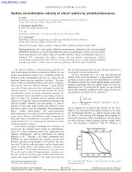
F is plotted versus φ s in figure 7 as a function of the
normalized excess carrier density, produced by illuminating
the device. The electric field is related to the charge density
through equation (10). Constant charge implies constant
R19