Lakeshore Model 331 Temperature Controller - Synchrotron ...

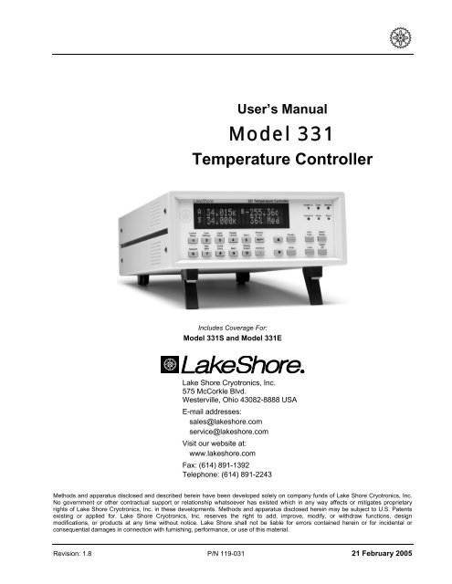
User’s Manual 

Model 331 

Temperature Controller 

Includes Coverage For: 

Model 331S and Model 331E 

Lake Shore Cryotronics, Inc. 

575 McCorkle Blvd. 

Westerville, Ohio 43082-8888 USA 

E-mail addresses: 

sales@lakeshore.com 

service@lakeshore.com 

Visit our website at: 

www.lakeshore.com 

Fax: (614) 891-1392 

Telephone: (614) 891-2243 

Methods and apparatus disclosed and described herein have been developed solely on company funds of Lake Shore Cryotronics, Inc. 

No government or other contractual support or relationship whatsoever has existed which in any way affects or mitigates proprietary 

rights of Lake Shore Cryotronics, Inc. in these developments. Methods and apparatus disclosed herein may be subject to U.S. Patents 

existing or applied for. Lake Shore Cryotronics, Inc. reserves the right to add, improve, modify, or withdraw functions, design 

modifications, or products at any time without notice. Lake Shore shall not be liable for errors contained herein or for incidental or 

consequential damages in connection with furnishing, performance, or use of this material. 

Revision: 1.8 P/N 119-031 21 February 2005

Lake Shore Model 331 Temperature Controller User’s Manual 

LIMITED WARRANTY STATEMENT 

WARRANTY PERIOD: ONE (1) YEAR 

1. Lake Shore warrants that this Lake Shore product (the 

“Product”) will be free from defects in materials and 

workmanship for the Warranty Period specified above (the 

“Warranty Period”). If Lake Shore receives notice of any such 

defects during the Warranty Period and the Product is shipped 

freight prepaid, Lake Shore will, at its option, either repair or 

replace the Product if it is so defective without charge to the 

owner for parts, service labor or associated customary return 

shipping cost. Any such replacement for the Product may be 

either new or equivalent in performance to new. Replacement or 

repaired parts will be warranted for only the unexpired portion of 

the original warranty or 90 days (whichever is greater). 

2. Lake Shore warrants the Product only if it has been sold by an 

authorized Lake Shore employee, sales representative, dealer 

or original equipment manufacturer (OEM). 

3. The Product may contain remanufactured parts equivalent to 

new in performance or may have been subject to incidental use. 

4. The Warranty Period begins on the date of delivery of the 

Product or later on the date of installation of the Product if the 

Product is installed by Lake Shore, provided that if you schedule 

or delay the Lake Shore installation for more than 30 days after 

delivery the Warranty Period begins on the 31st day after 

delivery. 

5. This limited warranty does not apply to defects in the Product 

resulting from (a) improper or inadequate maintenance, repair or 

calibration, (b) fuses, software and non-rechargeable batteries, 

(c) software, interfacing, parts or other supplies not furnished by 

Lake Shore, (d) unauthorized modification or misuse, (e) 

operation outside of the published specifications or (f) improper 

site preparation or maintenance. 

6. TO THE EXTENT ALLOWED BY APPLICABLE LAW, THE 

ABOVE WARRANTIES ARE EXCLUSIVE AND NO OTHER 

WARRANTY OR CONDITION, WHETHER WRITTEN OR 

ORAL, IS EXPRESSED OR IMPLIED. LAKE SHORE 

SPECIFICALLY DISCLAIMS ANY IMPLIED WARRANTIES OR 

CONDITIONS OF MERCHANTABILITY, SATISFACTORY 

QUALITY AND/OR FITNESS FOR A PARTICULAR PURPOSE 

WITH RESPECT TO THE PRODUCT. Some countries, states 

or provinces do not allow limitations on an implied warranty, so 

the above limitation or exclusion might not apply to you. This 

warranty gives you specific legal rights and you might also have 

other rights that vary from country to country, state to state or 

province to province. 

7. TO THE EXTENT ALLOWED BY APPLICABLE LAW, THE 

REMEDIES IN THIS WARRANTY STATEMENT ARE YOUR 

SOLE AND EXCLUSIVE REMEDIES. 

8. EXCEPT TO THE EXTENT PROHIBITED BY APPLICABLE 

LAW, IN NO EVENT WILL LAKE SHORE OR ANY OF ITS 

SUBSIDIARIES, AFFILIATES OR SUPPLIERS BE LIABLE FOR 

DIRECT, SPECIAL, INCIDENTAL, CONSEQUENTIAL OR 

OTHER DAMAGES (INCLUDING LOST PROFIT, LOST DATA 

OR DOWNTIME COSTS) ARISING OUT OF THE USE, 

INABILITY TO USE OR RESULT OF USE OF THE PRODUCT, 

WHETHER BASED IN WARRANTY, CONTRACT, TORT OR 

OTHER LEGAL THEORY, AND WHETHER OR NOT LAKE 

SHORE HAS BEEN ADVISED OF THE POSSIBILITY OF 

SUCH DAMAGES. Your use of the Product is entirely at your 

own risk. Some countries, states and provinces do not allow the 

exclusion of liability for incidental or consequential damages, so 

the above limitation may not apply to you. 

LIMITED WARRANTY STATEMENT (Continued) 

9. EXCEPT TO THE EXTENT ALLOWED BY APPLICABLE LAW, 

THE TERMS OF THIS LIMITED WARRANTY STATEMENT DO 

NOT EXCLUDE, RESTRICT OR MODIFY, AND ARE IN 

ADDITION TO, THE MANDATORY STATUTORY RIGHTS 

APPLICABLE TO THE SALE OF THE PRODUCT TO YOU. 

CERTIFICATION 

Lake Shore certifies that this product has been inspected and 

tested in accordance with its published specifications and that this 

product met its published specifications at the time of shipment. 

The accuracy and calibration of this product at the time of 

shipment are traceable to the United States National Institute of 

Standards and Technology (NIST); formerly known as the National 

Bureau of Standards (NBS). 

FIRMWARE LIMITATIONS 

Lake Shore has worked to ensure that the Model 331 firmware is 

as free of errors as possible, and that the results you obtain from 

the instrument are accurate and reliable. However, as with any 

computer-based software, the possibility of errors exists. 

In any important research, as when using any laboratory 

equipment, results should be carefully examined and rechecked 

before final conclusions are drawn. Neither Lake Shore nor anyone 

else involved in the creation or production of this firmware can pay 

for loss of time, inconvenience, loss of use of the product, or 

property damage caused by this product or its failure to work, or 

any other incidental or consequential damages. Use of our product 

implies that you understand the Lake Shore license agreement and 

statement of limited warranty. 

FIRMWARE LICENSE AGREEMENT 

The firmware in this instrument is protected by United States 

copyright law and international treaty provisions. To maintain the 

warranty, the code contained in the firmware must not be modified. 

Any changes made to the code is at the user’s risk. Lake Shore will 

assume no responsibility for damage or errors incurred as result of 

any changes made to the firmware. 

Under the terms of this agreement you may only use the Model 

331 firmware as physically installed in the instrument. Archival 

copies are strictly forbidden. You may not decompile, disassemble, 

or reverse engineer the firmware. If you suspect there are 

problems with the firmware, return the instrument to Lake Shore for 

repair under the terms of the Limited Warranty specified above. 

Any unauthorized duplication or use of the Model 331 firmware in 

whole or in part, in print, or in any other storage and retrieval 

system is forbidden. 

TRADEMARK ACKNOWLEDGMENT 

Many manufacturers and sellers claim designations used to 

distinguish their products as trademarks. Where those 

designations appear in this manual and Lake Shore was aware of 

a trademark claim, they appear with initial capital letters and the 

or ® symbol. 

CalCurve, Cernox, Duo-Twist, Quad-Lead, 

Quad-Twist, Rox, and SoftCal are trademarks 

of Lake Shore Cryotronics, Inc. 

MS-DOS ® and Windows/95/98/NT/2000 ® are trademarks of 

Microsoft Corp. 

NI-488.2 is a trademark of National Instruments. 

PC, XT, AT, and PS-2 are trademarks of IBM. 

Copyright © 2000 – 2002 & 2004 – 2005 by Lake Shore Cryotronics, Inc. All rights reserved. No portion of this manual 

may be reproduced, stored in a retrieval system, or transmitted, in any form or by any means, electronic, mechanical, 

photocopying, recording, or otherwise, without the express written permission of Lake Shore. 

A


DECLARATION OF CONFORMITY 

We: 

Lake Shore Cryotronics, Inc. 

575 McCorkle Blvd. 

Westerville OH 43082-8888 USA 

hereby declare that the equipment specified conforms to the following 

Directives and Standards: 

Application of Council Directives: .............................. 73/23/EEC 

89/336/EEC 

Standards to which Conformity is declared: .............. EN61010-1:2001 

Overvoltage II 

Pollution Degree 2 

EN61326 A2:2001 

Class A 

Annex B 

Model Number:.......................................................... 331 

Ed Maloof 

Printed Name 

Vice President of Engineering 

Position 

B


Electromagnetic Compatibility (EMC) for the Model 331 Temperature Controller 

Electromagnetic Compatibility (EMC) of electronic equipment is a growing concern worldwide. 

Emissions of and immunity to electromagnetic interference is now part of the design and manufacture 

of most electronics. To qualify for the CE Mark, the Model 331 meets or exceeds the requirements of 

the European EMC Directive 89/336/EEC as a CLASS A product. A Class A product is allowed to 

radiate more RF than a Class B product and must include the following warning: 

WARNING: 

This is a Class A product. In a domestic environment, this product may 

cause radio interference in which case the user may be required to take 

adequate measures. 

The instrument was tested under normal operating conditions with sensor and interface cables 

attached. If the installation and operating instructions in the User’s Manual are followed, there should 

be no degradation in EMC performance. 

This instrument is not intended for use in close proximity to RF Transmitters such as two-way radios 

and cell phones. Exposure to RF interference greater than that found in a typical laboratory 

environment may disturb the sensitive measurement circuitry of the instrument. 

Pay special attention to instrument cabling. Improperly installed cabling may defeat even the best 

EMC protection. For the best performance from any precision instrument, follow the grounding and 

shielding instructions in the User’s Manual. In addition, the installer of the Model 331 should consider 

the following: 

• Shield measurement and computer interface cables. 

• Leave no unused or unterminated cables attached to the instrument. 

• Make cable runs as short and direct as possible. Higher radiated emissions is possible with 

long cables. 

• Do not tightly bundle cables that carry different types of signals. 

C


TABLE OF CONTENTS 

Chapter/Paragraph Title Page 

1 INTRODUCTION .................................................................................................................................................... 1-1 

1.0 PRODUCT DESCRIPTION ............................................................................................................... 1-1 

1.1 SENSOR SELECTION ...................................................................................................................... 1-4 

1.2 SPECIFICATIONS............................................................................................................................. 1-6 

1.3 SAFETY SUMMARY ......................................................................................................................... 1-9 

1.4 SAFETY SYMBOLS ........................................................................................................................ 1-10 

2 COOLING SYSTEM DESIGN................................................................................................................................. 2-1 

2.0 GENERAL ......................................................................................................................................... 2-1 

2.1 TEMPERATURE SENSOR SELECTION .......................................................................................... 2-1 

2.1.1 Temperature Range....................................................................................................................... 2-1 

2.1.2 Sensor Sensitivity .......................................................................................................................... 2-1 

2.1.3 Environmental Conditions .............................................................................................................. 2-2 

2.1.4 Measurement Accuracy ................................................................................................................. 2-2 

2.1.5 Sensor Package............................................................................................................................. 2-2 

2.2 CALIBRATED SENSORS ................................................................................................................. 2-2 

2.2.1 Traditional Calibration .................................................................................................................... 2-2 

2.2.2 SoftCal........................................................................................................................................ 2-3 

2.2.3 Standard Curves ............................................................................................................................ 2-3 

2.2.4 CalCurve .................................................................................................................................... 2-3 

2.3 SENSOR INSTALLATION................................................................................................................. 2-5 

2.3.1 Mounting Materials......................................................................................................................... 2-5 

2.3.2 Sensor Location ............................................................................................................................. 2-5 

2.3.3 Thermal Conductivity ..................................................................................................................... 2-5 

2.3.4 Contact Area .................................................................................................................................. 2-5 

2.3.5 Contact Pressure ........................................................................................................................... 2-6 

2.3.6 Lead Wire....................................................................................................................................... 2-6 

2.3.7 Lead Soldering............................................................................................................................... 2-7 

2.3.8 Heat Sinking Leads........................................................................................................................ 2-7 

2.3.9 Thermal Radiation.......................................................................................................................... 2-7 

2.4 HEATER SELECTION AND INSTALLATION.................................................................................... 2-7 

2.4.1 Heater Resistance and Power ....................................................................................................... 2-7 

2.4.2 Heater Location.............................................................................................................................. 2-8 

2.4.3 Heater Types ................................................................................................................................. 2-8 

2.4.4 Heater Wiring ................................................................................................................................. 2-8 

2.5 CONSIDERATIONS FOR GOOD CONTROL ................................................................................... 2-8 

2.5.1 Thermal Conductivity ..................................................................................................................... 2-8 

2.5.2 Thermal Lag................................................................................................................................... 2-8 

2.5.3 Two-Sensor Approach ................................................................................................................... 2-9 

2.5.4 Thermal Mass ................................................................................................................................ 2-9 

2.5.5 System Nonlinearity ....................................................................................................................... 2-9 

2.6 PID CONTROL.................................................................................................................................. 2-9 

2.6.1 Proportional (P)............................................................................................................................ 2-10 

2.6.2 Integral (I)..................................................................................................................................... 2-10 

2.6.3 Derivative (D) ............................................................................................................................... 2-10 

2.6.4 Manual Heater Power (MHP) Output ........................................................................................... 2-10 

2.7 MANUAL TUNING........................................................................................................................... 2-12 

2.7.1 Setting Heater Range .................................................................................................................. 2-12 

2.7.2 Tuning Proportional...................................................................................................................... 2-12 

2.7.3 Tuning Integral ............................................................................................................................. 2-13 

2.7.4 Tuning Derivative ......................................................................................................................... 2-13 

2.8 AUTOTUNING................................................................................................................................. 2-13 

2.9 ZONE TUNING................................................................................................................................ 2-14 

Table of Contents 

i


TABLE OF CONTENTS (Continued) 


3 INSTALLATION...................................................................................................................................................... 3-1 

3.0 GENERAL ......................................................................................................................................... 3-1 

3.1 INSPECTION AND UNPACKING...................................................................................................... 3-1 

3.2 REPACKAGING FOR SHIPMENT ....................................................................................................3-1 

3.3 REAR PANEL DEFINITION............................................................................................................... 3-2 

3.4 LINE INPUT ASSEMBLY................................................................................................................... 3-3 

3.4.1 Line Voltage ................................................................................................................................... 3-3 

3.4.2 Line Fuse and Fuse Holder............................................................................................................ 3-3 

3.4.3 Power Cord .................................................................................................................................... 3-3 

3.4.4 Power Switch ................................................................................................................................. 3-4 

3.5 DIODE/RESISTOR SENSOR INPUTS.............................................................................................. 3-4 

3.5.1 Sensor Input Connector and Pinout ............................................................................................... 3-4 

3.5.2 Sensor Lead Cable ........................................................................................................................ 3-5 

3.5.3 Grounding and Shielding Sensor Leads......................................................................................... 3-5 

3.5.4 Sensor Polarity............................................................................................................................... 3-5 

3.5.5 Four-Lead Sensor Measurement ................................................................................................... 3-6 

3.5.6 Two-Lead Sensor Measurement.................................................................................................... 3-6 

3.5.7 Lowering Measurement Noise........................................................................................................ 3-6 

3.6 THERMOCOUPLE SENSOR INPUTS .............................................................................................. 3-7 

3.6.1 Sensor Input Terminals .................................................................................................................. 3-7 

3.6.2 Thermocouple Installation .............................................................................................................. 3-7 

3.6.3 Grounding and Shielding................................................................................................................ 3-7 

3.7 HEATER OUTPUT SETUP ............................................................................................................... 3-8 

3.7.1 Loop 1 Output ................................................................................................................................ 3-8 

3.7.2 Loop 1 Heater Output Connector ................................................................................................... 3-8 

3.7.3 Loop 1 Heater Output Wiring ......................................................................................................... 3-8 

3.7.4 Loop 1 Heater Output Noise .......................................................................................................... 3-9 

3.7.5 Loop 2 Output ................................................................................................................................ 3-9 

3.7.6 Loop 2 Output Resistance.............................................................................................................. 3-9 

3.7.7 Loop 2 Output Connector............................................................................................................... 3-9 

3.7.8 Loop 2 Heater Protection ............................................................................................................... 3-9 

3.7.9 Boosting the Output Power ............................................................................................................ 3-9 

3.8 ANALOG OUTPUT .......................................................................................................................... 3-10 

3.9 RELAYS .......................................................................................................................................... 3-10 

3.10 INITIAL SETUP AND SYSTEM CHECKOUT PROCEDURE .......................................................... 3-11 

4 OPERATION........................................................................................................................................................... 4-1 

4.0 GENERAL ......................................................................................................................................... 4-1 

4.1 FRONT PANEL DESCRIPTION ........................................................................................................ 4-1 

4.1.1 Keypad Definitions ......................................................................................................................... 4-1 

4.1.2 Annunciators .................................................................................................................................. 4-3 

4.1.3 General Keypad Operation ............................................................................................................ 4-3 

4.1.4 Display Definition ........................................................................................................................... 4-4 

4.2 TURNING POWER ON ..................................................................................................................... 4-4 

4.3 DISPLAY FORMAT AND SOURCE (UNITS) SELECTION ............................................................... 4-5 

4.4 INPUT SETUP................................................................................................................................... 4-7 

4.4.1 Diode Sensor Input Setup - 10 µA Excitation Current .................................................................... 4-7 

4.4.2 Diode Sensor Input Setup - 1 mA Excitation Current ..................................................................... 4-8 

4.4.3 Resistor Sensor Input Setup .......................................................................................................... 4-9 

4.4.3.1 Thermal EMF Compensation...................................................................................................... 4-9 

4.4.4 Thermocouple Sensor Input Setup............................................................................................... 4-10 

4.4.4.1 Room-Temperature Compensation .......................................................................................... 4-10 

4.4.4.2 Room-Temperature Calibration Procedure............................................................................... 4-11 

4.5 CURVE SELECTION....................................................................................................................... 4-12 

4.5.1 Diode Sensor Curve Selection ..................................................................................................... 4-13 

ii 

Table of Contents




4.5.2 Resistor Sensor Curve Selection ................................................................................................. 4-13 

4.5.3 Thermocouple Sensor Curve Selection ....................................................................................... 4-13 

4.6 TEMPERATURE CONTROL........................................................................................................... 4-14 

4.6.1 Control Loops............................................................................................................................... 4-14 

4.6.2 Control Modes.............................................................................................................................. 4-15 

4.6.3 Tuning Modes .............................................................................................................................. 4-15 

4.7 CONTROL SETUP .......................................................................................................................... 4-15 

4.8 MANUAL TUNING........................................................................................................................... 4-17 

4.8.1 Manually Setting Proportional (P) ................................................................................................ 4-17 

4.8.2 Manually Setting Integral (I) ......................................................................................................... 4-17 

4.8.3 Manually Setting Derivative (D).................................................................................................... 4-18 

4.8.4 Setting Manual Heater Power (MHP) Output ............................................................................... 4-18 

4.9 AUTOTUNE (CLOSED-LOOP PID CONTROL) .............................................................................. 4-19 

4.10 ZONE SETTINGS (CLOSED-LOOP CONTROL)............................................................................ 4-20 

4.11 SETPOINT....................................................................................................................................... 4-23 

4.12 RAMP .............................................................................................................................................. 4-24 

4.13 HEATER RANGE AND HEATER OFF ............................................................................................ 4-25 

4.14 MATH .............................................................................................................................................. 4-26 

4.14.1 Max/Min ....................................................................................................................................... 4-26 

4.14.2 Linear........................................................................................................................................... 4-27 

4.14.3 Filter............................................................................................................................................. 4-28 

4.15 ALARMS AND RELAYS .................................................................................................................. 4-29 

4.15.1 Alarms.......................................................................................................................................... 4-29 

4.15.2 Relays.......................................................................................................................................... 4-31 

4.16 ANALOG OUTPUT.......................................................................................................................... 4-32 

4.16.1 Analog Output In Input Mode ....................................................................................................... 4-32 

4.16.2 Analog Output In Manual Mode ................................................................................................... 4-34 

4.16.3 Analog Output In Loop 2 Mode .................................................................................................... 4-35 

4.17 LOCKING AND UNLOCKING THE KEYPAD.................................................................................. 4-35 

4.18 DISPLAY BRIGHTNESS ................................................................................................................. 4-36 

4.19 REMOTE/LOCAL ............................................................................................................................ 4-36 

4.20 INTERFACE .................................................................................................................................... 4-36 

4.21 DEFAULT VALUES ......................................................................................................................... 4-37 

5 ADVANCED OPERATION ..................................................................................................................................... 5-1 

5.0 GENERAL ......................................................................................................................................... 5-1 

5.1 CURVE NUMBERS AND STORAGE ................................................................................................ 5-1 

5.1.1 Curve Header Parameters ............................................................................................................. 5-1 

5.1.2 Curve Breakpoints ......................................................................................................................... 5-2 

5.2 FRONT PANEL CURVE ENTRY OPERATIONS .............................................................................. 5-2 

5.2.1 Edit Curve ...................................................................................................................................... 5-4 

5.2.1.1 Thermocouple Curve Considerations ......................................................................................... 5-5 

5.2.2 Erase Curve................................................................................................................................... 5-6 

5.2.3 Copy Curve.................................................................................................................................... 5-6 

5.3 SOFTCAL ...................................................................................................................................... 5-7 

5.3.1 SoftCal With Silicon Diode Sensors ............................................................................................... 5-7 

5.3.2 SoftCal Accuracy With Silicon Diode Sensors ...............................................................................5-8 

5.3.3 SoftCal With Platinum Sensors...................................................................................................... 5-9 

5.3.4 SoftCal Accuracy With Platinum Sensors ...................................................................................... 5-9 

5.3.5 SoftCal Calibration Curve Creation .............................................................................................. 5-10 

6 COMPUTER INTERFACE OPERATION................................................................................................................ 6-1 

6.0 GENERAL ......................................................................................................................................... 6-1 

6.1 IEEE-488 INTERFACE...................................................................................................................... 6-1 

6.1.1 IEEE-488 Interface Parameters ..................................................................................................... 6-2 

6.1.2 IEEE-488 Command Structure....................................................................................................... 6-2 


iii




6.1.2.1 Bus Control Commands ............................................................................................................. 6-2 

6.1.2.2 Common Commands.................................................................................................................. 6-3 

6.1.2.3 Device Specific Commands........................................................................................................ 6-3 

6.1.2.4 Message Strings......................................................................................................................... 6-3 

6.1.3 Status Registers............................................................................................................................. 6-4 

6.1.3.1 Status Byte Register and Service Request Enable Register ...................................................... 6-4 

6.1.3.2 Standard Event Status Register and Standard Event Status Enable Register ........................... 6-4 

6.1.4 IEEE Interface Example Programs................................................................................................. 6-5 

6.1.4.1 IEEE-488 Interface Board Installation for Visual Basic Program ................................................ 6-5 

6.1.4.2 Visual Basic IEEE-488 Interface Program Setup........................................................................ 6-7 

6.1.4.3 IEEE-488 Interface Board Installation for Quick Basic Program............................................... 6-10 

6.1.4.4 Quick Basic Program................................................................................................................ 6-10 

6.1.4.5 Program Operation ................................................................................................................... 6-13 

6.1.5 Troubleshooting ........................................................................................................................... 6-13 

6.2 SERIAL INTERFACE OVERVIEW .................................................................................................. 6-14 

6.2.1 Physical Connection..................................................................................................................... 6-14 

6.2.2 Hardware Support ........................................................................................................................ 6-14 

6.2.3 Character Format ......................................................................................................................... 6-15 

6.2.4 Message Strings .......................................................................................................................... 6-15 

6.2.5 Message Flow Control ................................................................................................................. 6-16 

6.2.6 Changing Baud Rate.................................................................................................................... 6-16 

6.2.7 Serial Interface Example Programs.............................................................................................. 6-17 

6.2.7.1 Visual Basic Serial Interface Program Setup............................................................................ 6-17 

6.2.7.2 Quick Basic Serial Interface Program Setup ............................................................................ 6-20 

6.2.7.3 Program Operation ................................................................................................................... 6-21 

6.2.8 Troubleshooting ........................................................................................................................... 6-21 

6.3 COMMAND SUMMARY .................................................................................................................. 6-22 

6.3.1 Interface Commands (Alphabetical Listing).................................................................................. 6-24 

7 OPTIONS AND ACCESSORIES ............................................................................................................................ 7-1 

7.0 GENERAL ......................................................................................................................................... 7-1 

7.1 MODELS ........................................................................................................................................... 7-1 

7.2 OPTIONS .......................................................................................................................................... 7-1 

7.3 ACCESSORIES................................................................................................................................. 7-2 

7.4 MODEL 3003 HEATER OUTPUT CONDITIONER............................................................................ 7-4 

8 SERVICE ................................................................................................................................................................ 8-1 

8.0 GENERAL ......................................................................................................................................... 8-1 

8.1 ELECTROSTATIC DISCHARGE....................................................................................................... 8-1 

8.1.1 Identification of Electrostatic Discharge Sensitive Components..................................................... 8-1 

8.1.2 Handling Electrostatic Discharge Sensitive Components............................................................... 8-1 

8.2 LINE VOLTAGE SELECTION ........................................................................................................... 8-2 

8.3 FUSE REPLACEMENT ..................................................................................................................... 8-2 

8.4 REAR PANEL CONNECTOR DEFINITIONS .................................................................................... 8-3 

8.4.1 Serial Interface Cable Wiring ......................................................................................................... 8-5 

8.4.2 IEEE-488 Interface Connector ....................................................................................................... 8-6 

8.5 TOP OF ENCLOSURE REMOVE AND REPLACE PROCEDURE.................................................... 8-7 

8.6 FIRMWARE AND NOVRAM REPLACEMENT .................................................................................. 8-7 

8.7 JUMPERS ......................................................................................................................................... 8-8 

8.8 ERROR MESSAGES......................................................................................................................... 8-8 

8.9 CALIBRATION PROCEDURE......................................................................................................... 8-10 

8.9.1 Equipment Required for Calibration ............................................................................................. 8-10 

8.9.2 Diode/Resistor Sensor Input Calibration ...................................................................................... 8-11 

8.9.2.1 Sensor Input Calibration Setup and Serial Communication Verification ................................... 8-11 

8.9.2.2 10 µA Current Source Calibration and 1 mA Current Source Verification................................. 8-11 

iv 

Table of Contents




8.9.2.3 Diode Input Ranges Calibration................................................................................................ 8-12 

8.9.2.4 Resistive Input Ranges Calibration .......................................................................................... 8-13 

8.9.3 Diode Sensor Input Calibration - 1 mA Excitation Current ........................................................... 8-14 

8.9.4 Thermocouple Sensor Input Calibration....................................................................................... 8-14 

8.9.4.1 Sensor Input Calibration Setup................................................................................................. 8-14 

8.9.4.2 Thermocouple Input Ranges Calibration .................................................................................. 8-14 

8.9.5 Analog Output Calibration (Model 331S Only) ............................................................................. 8-15 

8.9.5.1 Analog Output Calibration ........................................................................................................ 8-16 

8.9.6 Calibration Specific Interface Commands .................................................................................... 8-17 

APPENDIX A – GLOSSARY OF TERMINOLOGY........................................................................................................A-1 

APPENDIX B – TEMPERATURE SCALES ..................................................................................................................B-1 

APPENDIX C – HANDLING OF LIQUID HELIUM AND NITROGEN ............................................................................C-1 

APPENDIX D – CURVE TABLES .................................................................................................................................D-1 

LIST OF ILLUSTRATIONS 

Figure No. Title Page 

1-1 Model 331S Rear Panel Connections .......................................................................................................... 1-3 

2-1 Silicon Diode Sensor Calibrations and CalCurve ......................................................................................... 2-4 

2-2 Typical Sensor Installation In A Mechanical Refrigerator ............................................................................. 2-6 

2-3 Examples of PID Control ............................................................................................................................ 2-11 

3-1 Model 331 Rear Panel.................................................................................................................................. 3-2 

3-2 Line Input Assembly..................................................................................................................................... 3-3 

3-3 Diode/Resistor Input Connector ................................................................................................................... 3-4 

3-4 Thermocouple Input Definition and Common Connector Polarities.............................................................. 3-7 

3-5 RELAYS and ANALOG OUTPUT Terminal Block...................................................................................... 3-10 

4-1 Model 331 Front Panel ................................................................................................................................. 4-1 

4-2 Display Definition ......................................................................................................................................... 4-4 

4-3 Display Format Definition ............................................................................................................................. 4-5 

4-4 Record of Zone Settings............................................................................................................................. 4-22 

4-5 Deadband Example.................................................................................................................................... 4-29 

4-6 Relay Settings ............................................................................................................................................ 4-31 

5-1 SoftCal Temperature Ranges for Silicon Diode Sensors.............................................................................. 5-8 

5-2 SoftCal Temperature Ranges for Platinum Sensors..................................................................................... 5-9 

6-1 GPIB Setting Configuration .......................................................................................................................... 6-6 

6-2 DEV 12 Device Template Configuration....................................................................................................... 6-6 

6-3 Typical National Instruments GPIB Configuration from IBCONF.EXE........................................................ 6-11 

7-1 Model 331 Sensor and Heater Cable Assembly........................................................................................... 7-4 

7-2 Model 3003 Heater Output Conditioner........................................................................................................ 7-4 

7-3 Model RM-1/2 Rack-Mount Kit ..................................................................................................................... 7-5 

7-4 Model RM-2 Dual Rack-Mount Kit................................................................................................................ 7-6 

8-1 Power Fuse Access...................................................................................................................................... 8-2 

8-2 Sensor INPUT A and B Connector Details ................................................................................................... 8-3 

8-3 HEATER OUTPUT Connector Details.......................................................................................................... 8-3 

8-4 RELAYS and ANALOG OUTPUT Terminal Block........................................................................................ 8-4 

8-5 RS-232 Connector Details............................................................................................................................ 8-4 

8-6 IEEE-488 Rear Panel Connector Details...................................................................................................... 8-6 

8-7 Location of Internal Components ................................................................................................................. 8-9 

B-1 Temperature Scale Comparison ..................................................................................................................B-1 

C-1 Typical Cryogenic Storage Dewar................................................................................................................C-1 


v


LIST OF TABLES 

Table No. Title Page 

1-1 Sensor Temperature Range......................................................................................................................... 1-4 

1-2 Typical Sensor Performance ........................................................................................................................ 1-5 

1-3 Input Specifications ...................................................................................................................................... 1-6 

1-4 Sensor Input Configuration........................................................................................................................... 1-6 

1-5 Heater Output............................................................................................................................................... 1-7 

1-6 Loop 1 Full Scale Heater Power at Typical Resistance................................................................................ 1-7 

4-1 Sensor Input Types ...................................................................................................................................... 4-7 

4-2 Sensor Curves............................................................................................................................................ 4-12 

4-3 Comparison of Control Loops 1 and 2........................................................................................................ 4-14 

4-4 Linear Equation Configuration .................................................................................................................... 4-27 

4-5 Default Values ............................................................................................................................................ 4-38 

5-1 Curve Header Parameters............................................................................................................................ 5-3 

5-2 Recommended Curve Parameters ............................................................................................................... 5-3 

6-1 IEEE-488 Interface Program Control Properties........................................................................................... 6-8 

6-2 Visual Basic IEEE-488 Interface Program.................................................................................................... 6-9 

6-3 Quick Basic IEEE-488 Interface Program................................................................................................... 6-12 

6-4 Serial Interface Specifications .................................................................................................................... 6-15 

6-5 Serial Interface Program Control Properties............................................................................................... 6-18 

6-6 Visual Basic Serial Interface Program ........................................................................................................ 6-19 

6-7 Quick Basic Serial Interface Program......................................................................................................... 6-20 

6-8 Command Summary .................................................................................................................................. 6-23 

8-1 Calibration Table for Diode Ranges ........................................................................................................... 8-12 

8-2 Calibration Table for Resistive Ranges ...................................................................................................... 8-14 

8-3 Calibration Table for Thermocouple Ranges.............................................................................................. 8-15 

B-1 Temperature Conversion Table....................................................................................................................B-2 

C-1 Comparison of Liquid Helium and Liquid Nitrogen ...................................................................................... C-1 

D-1 DT-470 Silicon Diode Curve ........................................................................................................................ D-1 

D-2 DT-670 Silicon Diode Curve ........................................................................................................................ D-2 

D-3 DT-500 Series Silicon Diode Curves ........................................................................................................... D-2 

D-4 PT-100/-1000 Platinum RTD Curves........................................................................................................... D-3 

D-5 RX-102A Rox Curve ................................................................................................................................ D-4 

D-6 RX-202A Rox Curve ................................................................................................................................ D-5 

D-7 Type K Thermocouple Curve....................................................................................................................... D-6 

D-8 Type E Thermocouple Curve....................................................................................................................... D-7 

D-9 Type T Thermocouple Curve....................................................................................................................... D-8 

D-10 Chromel-AuFe 0.03% Thermocouple Curve................................................................................................ D-9 

D-11 Chromel-AuFe 0.07% Thermocouple Curve...............................................................................................D-10 

vi 

Table of Contents


CHAPTER 1 

INTRODUCTION 

1.0 PRODUCT DESCRIPTION 

The Model 331 Temperature Controller combines the easy operation and unsurpassed reliability of the 

Model 330 with improved sensor input and interface flexibility, including compatibility with negative 

temperature coefficient (NTC) resistance temperature detectors (RTDs). Backed by the Lake Shore 

tradition of excellence in cryogenic sensors and instrumentation, the Model 331 Temperature Controller 

sets the standard for mid-price range temperature control instruments. 

The Model 331 Temperature Controller is available in two versions. The Model 331S is fully equipped 

for interface and control flexibility. The Model 331E shares measurement and display capability with the 

Model 331S, but does not include the IEEE-488 interface, relays, analog voltage output, or a second 

control loop. 

Sensor Inputs 

The Model 331 Temperature Controller is designed for high performance over a wide operating 

temperature range and in difficult sensing conditions. The Model 331 features two inputs, with a highresolution 

24-bit analog-to-digital converter and separate current source for each input. Sensors are 

optically isolated from other instrument functions for quiet and repeatable sensor measurements. 

Sensor data from each input can be read up to ten times per second, with display updates twice each 

second. The Model 331 uses current reversal to eliminate thermal EMF errors in resistance sensors. 

Standard temperature response curves for silicon diodes, platinum RTDs, and many thermocouples are 

included. Up to twenty 200-point CalCurves for Lake Shore calibrated sensors or user curves can be 

loaded into non-volatile memory via a computer interface or the instrument front panel. A built-in 

SoftCal 1 algorithm can also be used to generate curves for silicon diodes and platinum RTDs, for 

storage as user curves. 

1 The Lake Shore SoftCal algorithm for silicon diode and platinum RTD sensors is a good solution for applications 

requiring more accuracy than a standard sensor curve but not in need of traditional calibration. SoftCal uses the 

predictability of a standard curve to improve the accuracy of an individual sensor around a few known temperature 

reference points. Both versions of the Model 331 can generate SoftCal curves. 

Introduction 1-1


Product Description (Continued) 

Sensor inputs for both versions of the Model 331 are factory configured and compatible with either 

diode/RTDs or thermocouple sensors. The purchaser’s choice of two diode/RTD inputs, one diode/RTD 

input and one thermocouple input, or two thermocouple inputs must be specified at time of order and 

cannot be reconfigured in the field. Software selects appropriate excitation current and signal gain 

levels when sensor type is entered via the instrument front panel. 

Temperature Control 

The Model 331E offers one and the Model 331S offers two proportional-integral-derivative (PID) control 

loops. A PID control algorithm calculates control output based on temperature setpoint and feedback 

from the control sensor. Wide tuning parameters accommodate most cryogenic cooling systems and 

many small high-temperature ovens. Control output is generated by a high-resolution digital-to-analog 

converter for smooth continuous control. The user can set the PID values or the Autotuning feature of 

the Model 331 can automate the tuning process. 

Heater output for Model 331S and Model 331E is a well-regulated variable DC current source. Heater 

output is optically isolated from other circuits to reduce interference and ground loops. Heater output 

can provide up to 50 W of continuous power to a resistive heater load, and includes two lower ranges 

for systems with less cooling power. Heater output is short-circuit protected to prevent instrument 

damage if the heater load is accidentally shorted. 

The setpoint ramp feature allows smooth continuous changes in setpoint and can also make the 

approach to a setpoint temperature more predictable. The zone feature can automatically change 

control parameter values for operation over a large temperature range. Values for ten different 

temperature zones can be loaded into the instrument, which will select the next appropriate value on 

setpoint change. 

Interface 

The Model 331 is available with both parallel (IEEE-488, 331S only) and serial (RS-232C) computer 

interfaces. In addition to data gathering, nearly every function of the instrument can be controlled via 

computer interface. Also included is a Model 330 command emulation mode that makes the Model 331 

interchangeable with the older Model 330 in software controlled systems. 

Each input has a high and low alarm which offer latching and non-latching operation. The two relays on 

the Model 331S can be used in conjunction with the alarms to alert the operator of a fault condition or 

perform simple on-off control. Relays can be assigned independently to any alarm or be operated 

manually. 

When not being used for temperature control, the loop 2 control output can be used as an analog 

voltage output. It can be configured to send a voltage proportional to temperature to a strip-chart 

recorder or data acquisition system. The user may select the scale and data sent to the output, 

including temperature, sensor units, or linear equation results. Under manual control, the analog 

voltage output can also serve as a voltage source for other applications. 

Interface Features of Model 331S and Model 331E 

Feature 331S 331E 

Numeric keypad • • 

Front panel curve entry • • 

Alarms • • 

RS-232C interface • • 

IEEE-488 interface • 

Second control loop • 

Analog voltage output • 

Two relays 

• 

1-2 Introduction


Line input assembly 

Serial (RS-232C) I/O (DTE) 

Heater output 

IEEE-488 interface 

Terminal block (for relays and analog output) 

Sensor input connectors 

Figure 1-1. Model 331S Rear Panel Connections 

Configurable Display 

Both versions of the Model 331 include a bright vacuum fluorescent display that simultaneously 

displays up to four readings. Display data includes input and source annunciators for each reading. All 

four display locations can be configured by the user. Data from either input may be assigned to any of 

the four locations; the user’s choice of temperature, sensor units, maximum, minimum, or linear 

equation results can be displayed. Heater range and control output as current or power can also be 

continuously displayed for immediate feedback on control operation. 

Normal (Default) Display Configuration 

The display provides four reading locations. Readings from each input and the control setpoint can be 

expressed in any combination of temperature or sensor units, with heater output expressed as a 

percent of full scale current or power. 

Flexible Configuration 

Reading locations can be configured by the user to meet application needs. The character preceding 

the reading indicates input A or B or setpoint S. The character following the reading indicates 

measurement units or the math function in use. 

Curve Entry 

The Model 331 display offers the flexibility to support curve, SoftCal, and zone entry. Curve entry 

may be performed accurately and to full resolution via the display and keypad as well as computer 

interface. 

Introduction 1-3


1.1 SENSOR SELECTION 

Table 1-1. Sensor Temperature Range 

Diodes 

Positive 

Temperature 

Coefficient RTDs 

Negative 


Coefficient 

RTDs 2 

Thermocouples 

Model Useful Range Magnetic Field Use 

Silicon Diode DT-670-SD 1.4 K to 500 K T ≥ 60 K & B ≤ 3 T 

Silicon Diode DT-670E-BR 30 K to 500 K T ≥ 60 K & B ≤ 3 T 

Silicon Diode DT-414 1.4 K to 375 K T ≥ 60 K & B ≤ 3 T 

Silicon Diode DT-421 1.4 K to 325 K T ≥ 60 K & B ≤ 3 T 

Silicon Diode DT-470-SD 1.4 K to 500 K T ≥ 60 K & B ≤ 3 T 

Silicon Diode DT-471-SD 10 K to 500 K T ≥ 60 K & B ≤ 3 T 

GaAlAs Diode TG-120-P 1.4 K to 325 K T > 4.2 K & B ≤ 5 T 

GaAlAs Diode TG-120-PL 1.4 K to 325 K T > 4.2 K & B ≤ 5 T 

GaAlAs Diode TG-120-SD 1.4 K to 500 K T > 4.2 K & B ≤ 5 T 

100 Ω Platinum PT-102/3 14 K to 873 K T > 40 K & B ≤ 2.5 T 

100 Ω Platinum PT-111 14 K to 673 K T > 40 K & B ≤ 2.5 T 

Rhodium-Iron RF-800-4 1.4 K to 500 K T > 77 K & B ≤ 8 T 

Rhodium-Iron RF-100T/U 1.4 K to 325 K T > 77 K & B ≤ 8 T 

Cernox CX-1010 2 K to 325 K 5 T > 2 & B ≤ 19 T 

Cernox CX-1030-HT 3.5 K to 420 K 3,6 T > 2 & B ≤ 19 T 

Cernox CX-1050-HT 4 K to 420 K 3,6 T > 2 & B ≤ 19 T 

Cernox CX-1070-HT 15 K to 420 K 3 T > 2 & B ≤ 19 T 

Cernox CX-1080-HT 50 K to 420 K 3 T > 2 & B ≤ 19 T 

Germanium GR-200A/B-1000 2.2 K to 100 K 4 Not Recommended 



Carbon-Glass CGR-1-500 4 K to 325 K 5 T > 2 K to ≤ 19 T 



Rox RX-102A 1.4 K to 40 K 5 T > 2 K to ≤ 10 T 

Type K 9006-006 3.2 K to 1505 K Not Recommended 

Type E 9006-004 3.2 K to 934 K Not Recommended 

Chromel-AuFe 0.07% 9006-002 1.2 K to 610 K Not Recommended 

2 Single excitation current may limit the low temperature range of NTC resistors. 

3 Non-HT version maximum temperature: 325 K. 

4 Low temperature limited by input resistance range. 

5 Low temperature specified with self-heating error: ≤5 mK. 

6 Low temperature specified with self-heating error: ≤12 mK. 

Silicon diodes are the best choice for general cryogenic use from 1.4 K to above room temperature. 

Diodes are economical to use because they follow a standard curve and are interchangeable in many 

applications. They are not suitable for use in ionizing radiation or magnetic fields. 

Cernox thin-film RTDs offer high sensitivity and low magnetic field-induced errors over the 2 K to 

420 K temperature range. Cernox sensors require calibration. 

Platinum RTDs offer high uniform sensitivity from 30 K to over 800 K. With excellent reproducibility, 

they are useful as thermometry standards. They follow a standard curve above 70 K and are 

interchangeable in many applications. 

1-4 Introduction


Silicon Diode 

Silicon Diode 

GaAlAs 

Diode 

100 Ω 

Platinum 

RTD 500 Ω 

Full Scale 

Cernox 

Germanium 

Carbon- 

Glass 

Thermocouple 

50mV 

Example Lake 

Shore Sensor 

DT-670-SD-13 

with 1.4H 

calibration 

DT-470-SD-13 

with 1.4H 

calibration 

TG-120-SD 

with 1.4H 

calibration 

PT-103 with 

1.4J calibration 

CX-1050-SD- 

HT 9 with 4M 

calibration 

GR-200A-1000 

with 1.4D 

calibration 

CGR-1-2000 

with 4L 

calibration 

Type K 

Temp 

Table 1-2. Typical Sensor Performance 

Nominal 

Resistance/ 

Voltage 

Typical Sensor 

Sensitivity 7 

Measurement 

Resolution: 


Equivalents 

Electronic 

Accuracy: 


Equivalents 


Accuracy 

including 

Electronic 

Accuracy, 

CalCurve, and 

Calibrated 

Sensor 

Electronic 

Control 

Stability 8 : 


Equivalents 

1.4 K 1.644 V -12.49 mV/K 0.8 mK ±13 mK ±25 mK ±1.6 mK 

77 K 1.028 V -1.73 mV/K 5.8 mK ±76 mK ±98 mK ±11.6 mK 









300 K 0.8978 V -2.85 mV/K 7 mK ±60 mK ±92 mK ±14 mK 


30 K 3.660 Ω 0.191 Ω/K 10.5 mK ±23 mK ±33 mK ±21 mK 

77 K 20.38 Ω 0.423 Ω/K 4.8 mK ±15 mK ±27 mK ±9.6 mK 

300 K 110.35 Ω 0.387 Ω/K 5.2 mK ±39 mK ±62 mK ±10.4 mK 

500 K 185.668 Ω 0.378 Ω/K 5.3 mK ±60 mK ±106 mK ±10.6 mK 

4.2 K 3507.2 Ω -1120.8 Ω/K 36 µK ±1.4 mK ±6.4 mK ±72 µK 

77 K 205.67 Ω -2.4116 Ω/K 16.6 mK ±76 mK ±92 mK ±33.2 mK 

300 K 59.467 Ω -0.1727 Ω/K 232 mK ±717 mK ±757 mK ±464 mK 

420 K 45.030 Ω -0.0829 Ω/K 483 mK ±1.42 K ±1.49 K ±966 mK 

2 K 6674 Ω -9930 Ω/K 4 µK ±0.3 mK ±4.3 mK ±8 µK 

4.2 K 1054 Ω -526 Ω/K 76 µK ±1 mK ±5 mK ±152 µK 

10 K 170.9 Ω -38.4 Ω/K 1 mK ±4.4 mK ±9.4 mK ±2 mK 

100 K 2.257 Ω -0.018 Ω/K 2.22 K ±5.61 K ±5.626 K ±4.44 K 

4.2 K 2260 Ω -2060 Ω/K 20 µK ±0.5 mK ±4.5 mK ±40 µK 

77 K 21.65 Ω -0.157 Ω/K 255 mK ±692 mK ±717 mK ±510 mK 

300 K 11.99 Ω -0.015 Ω/K 2.667 K ±7 K ±7.1 K ±5.344 K 

75 K -5862.9 µV 15.6 µV/K 26 mK ±0.25 K 10 ±52 mK 

300 K 1075.3 µV 40.6 µV/K 10 mK ±0.038 K 10 Calibration not 

±20 mK 

available from 

600 K 13325 µV 41.7 µV/K 10 mK ±0.184 K 10 Lake Shore ±20 mK 

1505 K 49998.3 µV 36.006 µV/K 12 mK ±0.73 K 10 

±24 mK 

7 Typical sensor sensitivities were taken from representative calibrations for the sensor listed 

8 Control stability of the electronics only, in an ideal thermal system 

9 Non-HT version maximum temperature: 325 K 

10 Accuracy specification does not include errors from room temperature compensation 

Introduction 1-5


1.2 SPECIFICATIONS 

Diode 

PTC RTD 

Table 1-3. Input Specifications 

Sensor 

Electronic 

Display Measurement 

Temperature Input Range Excitation Current 

Electronic Accuracy Control 

Resolution Resolution 

Coefficient 

Stability 11 

negative 0 V to 2.5 V 10 µA ±0.05% 12,13 100 µV 10 µV ±80 µV ±0.005% of rdg ±20 µV 

negative 0 V to 7.5 V 10 µA ±0.05% 12,13 100 µV 20 µV ±80 µV ±0.01% of rdg ±40 µV 

positive 0 Ω to 500 Ω 1 mA 14 10 mΩ 2 mΩ ±0.004 Ω ±0.01% of rdg ±4 mΩ 

positive 0 Ω to 5000 Ω 1 mA 14 100 mΩ 20 mΩ ±0.04 Ω ±0.02% of rdg ±40 mΩ 

NTC RTD negative 0 Ω to 7500 Ω 10 µA ±0.05% 14 100 mΩ 40 mΩ ±0.1 Ω ±0.04% of rdg ±80 mΩ 

Thermocouple positive ±25 mV NA 1 µV 0.4 µV ±1 µV ±0.05% of rdg 15 ±0.8 µV 

positive ±50 mV NA 1 µV 0.4 µV ±1 µV ±0.05% of rdg 15 ±0.8 µV 

11 Control stability of the electronics only, in an ideal thermal system 

12 Current source error has negligible effect on measurement accuracy 

13 Diode input excitation can be set to 1 mA – refer to Paragraph 4.4.2 

14 Current source error is removed during calibration 

15 Accuracy specification does not include errors from room temperature compensation 

Thermometry 

Number of inputs 2 

Input configuration Each input is factory configured for either diode/RTD or thermocouples 

Isolation 

Sensor inputs optically isolated from other circuits but not each other 

A/D resolution 

24-bit 

Input accuracy 

Sensor dependent – refer to Input Specifications table 

Measurement resolution Sensor dependent – refer to Input Specifications table 

Maximum update rate 10 readings/s on each input (except 5 readings/s on input A when configured 

as thermocouple) 

User curves 

Room for twenty 200-point CalCurves or user curves 

SoftCal 

Improves accuracy of DT-470 diode to ±0.25 K from 30 K to 375 K; improves 

accuracy of Platinum RTDs to ±0.25 K from 70 K to 325 K – stored as user 

curves 

Math 

Maximum, Minimum, and Linear Equation (Mx + B) or M(x+B) 

Filter 

Averages 2 to 64 input readings 

Table 1-4. Sensor Input Configuration 

Diode/RTD 

Thermocouple 

Measurement type 4-lead differential 2-lead, room temperature compensated 

Excitation 

Constant current with current reversal for 

RTDs 

NA 

Supported sensors 

Standard curves 

Diodes: Silicon, GaAlAs RTDs: 100 Ω 

Platinum, 1000 Ω Platinum, Germanium, 

Carbon-Glass, Cernox, and Rox 

DT-470, DT-500D, DT-670, PT-100, PT- 

1000, RX-102A, RX-202A 

Most thermocouple types 

Type E, Type K, Type T, AuFe 0.07% 

vs. Cr, AuFe 0.03% vs. Cr 

Input connector 6-pin DIN Ceramic isothermal block 

1-6 Introduction


Specifications (Continued) 

Control 

Control loops 

Control type 

Tuning 

Control stability 

PID control parameters 

Proportional (gain) 

Integral (reset) 

Derivative (rate) 

Manual output 

Zone control 

Setpoint ramping 

Safety limits 

Two on 331S, one on 331E 

Closed loop digital PID with manual heater output, or open loop 

Autotune (one loop at a time), PID, PID zones 

Sensor dependent – to 2× measurement resolution 

(in an ideal thermal system) 

0 to 1000 with 0.1 setting resolution 

1 to 1000 (1000/s) with 0.1 setting resolution 

1 to 200% with 1% resolution 

0 to 100% with 0.01% setting resolution 

10 temperature zones with P, I, D, manual heater out, and heater range 

0.1 K/min to 100 K/min 

Curve temperature, power up heater off, short circuit protection 

Table 1-5. Heater Output 

Loop 1 Loop 2 

Heater output type Variable DC current source Variable DC voltage source 

Heater output D/A resolution 18-bit 16-bit 

Max heater power 50 W 1 W 

Max heater output current 1 A 0.1 A 

Heater output compliance 50 V 10 V 

Heater output ranges 3 decade steps in power 1 

Heater load type Resistive Resistive 

Heater load range 10 Ω to 100 Ω recommended 100 Ω minimum 

Heater load for max power 50 Ω 100 Ω 

Heater noise (



Front Panel 

Display 

2 line by 20 character, 9 mm character height, vacuum fluorescent 

display 

Number of reading displays 1 to 4 

Display units 

K, °C, V, mV, Ω 

Reading source 

Temperature, sensor units, max, min, and linear equation 

Display update rate 

All readings twice per s 

Temp display resolution 0.001° from 0° to 99.999°, 0.01° from 100° to 999.99°, 

0.1° above 1000° 

Sensor units display resolution Sensor dependent to 5 digits 

Other displays 

Setpoint, Heater Range, and Heater Output (user selected) 

Setpoint setting resolution Same as display resolution (actual resolution is sensor dependent) 

Heater output display Numeric display in percent of full scale for power or current 

Heater output resolution 1% 

Display annunciators 

Control Input, Remote, Alarm, Tuning, Ramp, Max, Min, Linear 

Keypad 

20 full travel keys, numeric and specific functions 

Front panel features 

Front panel curve entry, display brightness control, keypad lock-out 

Interface 

IEEE-488 interface (331S) 

Features 

Reading rate 

Software support 

Serial interface 

Electrical format 

Max baud rate 

Connector 

Reading rate 

Special interface features 

Alarms 

Number 

Data source 

Settings 

SH1, AH1, T5, L4, SR1, RL1, PP0, DC1, DT0, C0, E1 

To 10 readings per s on each input 

LabVIEW driver (consult factory for availability) 

RS-232C 

9600 baud 

9-pin D-sub 

To 10 readings/s on each input (at 9600 baud) 

Model 330 command emulation mode 

4, high and low for each input 

Temperature, Sensor Units, Linear Equation 

Source, High Setpoint, Low Setpoint, Deadband, Latching or Non- 

Latching, Audible On/Off 

Actuators 

Display annunciator, beeper, relays 

Relays (331S) 

Number 2 

Contacts 

Normally Open (NO), Normally Closed (NC), and Common (C) 

Contact rating 

30 VDC at 5 A 

Operation 

Activate relays on high, low, or both alarms for either input or manual 

Connector 

Detachable terminal block 

Analog voltage output (331S) 

Scale 

User selected 

Update rate 

10 readings per s 

Data source 

Temperature, Sensor Units, Linear Equation 

Settings 

Input, source, top of scale, bottom of scale, or manual 

Range 

±10 V 

Resolution 

0.3 mV 

Accuracy 

±2.5 mV 

Min load resistance 100 Ω (short circuit protected) 

1-8 Introduction



General 

Ambient temperature 

Power requirement 

Size 

Weight 

Approval 

15 °C to 35 °C at rated accuracy, 10 °C to 40 °C at reduced accuracy 

100, 120, 220, 240 VAC, (+6%, -10%), 50 or 60 Hz, 120 VA 

216 mm W × 89 mm H × 368 mm D (8.5 in × 3.5 in × 14.5 in), half rack 

4.8 kg (10.5 lb) 

CE mark 

Product Configuration 

Part Number 

Description (Input configuration cannot be changed in the field) 

Standard Temperature Controllers, all features included: 

331S 

Two Diode/Resistor Inputs 

331S-T1 

One Diode/Resistor, One Thermocouple Input 

331S-T2 

Two Thermocouple Inputs 

Economy Temperature Controllers, all features of the 331S except does not include the following: 

IEEE-488, relays, analog voltage output, second control loop. 

331E 

Two Diode/Resistor Inputs 

331E-T1 

One Diode/Resistor, One Thermocouple Input 

331E-T2 

Two Thermocouple Inputs 

Refer to Chapter 7 of this manual for a complete description of Model 331 options and accessories. 

Specifications subject to change without notice. 

1.3 SAFETY SUMMARY 

Observe these general safety precautions during all phases of instrument operation, service, and 

repair. Failure to comply with these precautions or with specific warnings elsewhere in this manual 

violates safety standards of design, manufacture, and intended instrument use. Lake Shore 

Cryotronics, Inc. assumes no liability for Customer failure to comply with these requirements. 

The Model 331 protects the operator and surrounding area from electric shock or burn, mechanical 

hazards, excessive temperature, and spread of fire from the instrument. Environmental conditions 

outside of the conditions below may pose a hazard to the operator and surrounding area. 

• Indoor use. 

• Altitude to 2000 meters. 

• Temperature for safe operation: 5 °C to 40 °C. 

• Maximum relative humidity: 80% for temperature up to 31 °C decreasing linearly to 50% at 40 °C. 

• Power supply voltage fluctuations not to exceed ±10% of the nominal voltage. 

• Overvoltage category II. 

• Pollution degree 2. 

Ground The Instrument 

To minimize shock hazard, the instrument is equipped with a three-conductor AC power cable. Plug the 

power cable into an approved three-contact electrical outlet or use a three-contact adapter with the 

grounding wire (green) firmly connected to an electrical ground (safety ground) at the power outlet. 

The power jack and mating plug of the power cable meet Underwriters Laboratories (UL) and 

International Electrotechnical Commission (IEC) safety standards. 

Introduction 1-9


Safety Summary (Continued) 

Ventilation 

The instrument has ventilation holes in its side covers. Do not block these holes when the instrument is 

operating. 

Do Not Operate In An Explosive Atmosphere 

Do not operate the instrument in the presence of flammable gases or fumes. Operation of any electrical 

instrument in such an environment constitutes a definite safety hazard. 

Keep Away From Live Circuits 

Operating personnel must not remove instrument covers. Refer component replacement and internal 

adjustments to qualified maintenance personnel. Do not replace components with power cable 

connected. To avoid injuries, always disconnect power and discharge circuits before touching them. 

Do Not Substitute Parts Or Modify Instrument 

Do not install substitute parts or perform any unauthorized modification to the instrument. Return the 

instrument to an authorized Lake Shore Cryotronics, Inc. representative for service and repair to ensure 

that safety features are maintained. 

Cleaning 

Do not submerge instrument. Clean only with a damp cloth and mild detergent. Exterior only. 

1.4 SAFETY SYMBOLS 

1-10 Introduction


CHAPTER 2 

COOLING SYSTEM DESIGN 

2.0 GENERAL 

Selecting the proper cryostat or cooling source is probably the most important decision in designing a 

temperature control system. The cooling source defines minimum temperature, cool-down time, and 

cooling power. (Information on choosing a cooling source is beyond the scope of this manual.) This 

chapter provides information on how to get the best temperature measurement and control from cooling 

sources with proper setup including sensor and heater installation. 

Chapter 2 contains the following major topics. Temperature sensor selection is covered in 

Paragraph 2.1. Calibrated sensors are covered in Paragraph 2.2. Sensor installation is covered in 

Paragraph 2.3. Heater selection and installation is covered in Paragraph 2.4. Considerations for good 

control are covered in Paragraph 2.5. PID Control is covered in Paragraph 2.6. Manual Tuning is 

covered in Paragraph 2.7. AutoTuning is covered in Paragraph 2.8. Finally, Zone Tuning is covered in 

Paragraph 2.9. 

2.1 TEMPERATURE SENSOR SELECTION 

This section attempts to answer some of the basic questions concerning temperature sensor selection. 

Additional useful information on temperature sensor selection is available in the Lake Shore 

Temperature Measurement and Control Catalog. The catalog has a large reference section that 

includes sensor characteristics and sensor selection criteria. 

2.1.1 Temperature Range 

Several important sensor parameters must be considered when choosing a sensor. The first is 

temperature range. The experimental temperature range must be known when choosing a sensor. 

Some sensors can be damaged by temperatures that are either too high or too low. Manufacturer 

recommendations should always be followed. 

Sensor sensitivity is also dependent on temperature and can limit the useful range of a sensor. It is 

important not to specify a range larger than necessary. If an experiment is being done at liquid helium 

temperature, a very high sensitivity is needed for good measurement resolution at that temperature. 

That same resolution may not be required to monitor warm up to room temperature. Two different 

sensors may be required to tightly cover the range from helium to room temperature, but lowering the 

resolution requirement on warm up may allow a less expensive, one sensor solution. 

Another thing to consider when choosing a temperature sensor is that instruments like the Model 331 

are not able to read some sensors over their entire temperature range. Lake Shore sells calibrated 

sensors that operate down to 50 millikelvin (mK), but the Model 331 is limited to above 1 K in its 

standard configuration. 

2.1.2 Sensor Sensitivity 

Temperature sensor sensitivity is a measure of how much a sensor signal changes when the 

temperature changes. It is an important sensor characteristic because so many measurement 

parameters are related to it. Resolution, accuracy, noise floor, and even control stability depend on 

sensitivity. Many sensors have different sensitivities at different temperatures. For example, a 

platinum sensor has good sensitivity at higher temperatures but has limited use below 30 kelvin (K) 

because its sensitivity drops sharply. It is difficult to determine if a sensor has adequate sensitivity 

over the experimental temperature range. This manual has specifications (Table 1-3) that include 

sensor sensitivity translated into temperature resolution and accuracy at different points. This is 

typical sensor response and can be used as a guide when choosing a sensor to be used with the 

Model 331. 

Cooling System Design 2-1


2.1.3 Environmental Conditions 

The experimental environment is also important when choosing a sensor. Environmental factors such 

as high vacuum, magnetic field, corrosive chemicals, or even radiation can limit the use of some 

types of sensors. Lake Shore has devoted much time to developing sensor packages that withstand 

the temperatures, vacuum levels, and bonding materials found in typical cryogenic cooling systems. 

Experiments done in magnetic fields are becoming very common. Field dependence of temperature 

sensors is an important selection criteria for sensors used in these experiments. This manual briefly 

qualifies the field dependence of most common sensors in the specifications (Table 1-3). Detailed 

field dependence tables are included in the Lake Shore Temperature Measurement and Control 

Catalog. When available, specific data on other environmental factors is also included in the catalog. 

2.1.4 Measurement Accuracy 

Temperature measurements have several sources of error that reduce accuracy. Be sure to account 

for errors induced by both the sensor and the instrumentation when computing accuracy. The 

instrument has measurement error in reading the sensor signal and error in calculating a temperature 

using a temperature response curve. Error results from the sensor being compared to a calibration 

standard and the temperature response of a sensor will shift with time and with repeated thermal 

cycling (from very cold temperatures to room temperature). Instrument and sensor makers specify 

these errors but there are things a user can do to maintain good accuracy. For example, choose a 

sensor that has good sensitivity in the most critical temperature range, as sensitivity can minimize the 

effect of most error sources. Install the sensor properly following guidelines in Paragraph 2.3. Have 

the sensor and instrument periodically recalibrated, or in some other way null the time dependent 

errors. Use a sensor calibration that is appropriate for the accuracy requirement. 

2.1.5 Sensor Package 

Many types of sensors can be purchased in different packages. Some types of sensors can even be 

purchased as bare chips; without any package. A sensor package generally determines its size, 

thermal and electrical contact to the outside, and sometimes limits temperature range. When different 

packages are available for a sensor, the user should consider the mounting surface for the sensor 

and how leads will be heat sinked when choosing. 

2.2 CALIBRATED SENSORS 

There can sometimes be confusion in the difficult task of choosing the right sensor, getting it calibrated, 

translating the calibration data into a temperature response curve that the Model 331 can understand, 

then getting the curve loaded into the instrument. Lake Shore provides a variety of calibration and curve 

loading services to fit different accuracy requirements and budgets. 

2.2.1 Traditional Calibration 

Calibration is done by comparing a sensor with an unknown temperature response to an accepted 

standard. Lake Shore temperature standards are traceable to the U.S. National Institute of Standards 

and Testing (NIST) or the National Physical Laboratory in Great Britain. These standards allow Lake 

Shore to calibrate sensors from 50 mK to above room temperature. Calibrated sensors are more 

expensive than uncalibrated sensors of the same type because of the labor and capitol equipment 

used in the process. 

This type of calibration provides the most accurate temperature sensors available from Lake Shore. 

Errors from sensor calibration are almost always smaller than the error contributed by the Model 331. 

The Lake Shore Temperature Measurement and Control Catalog has complete accuracy 

specifications for calibrated sensors. 

2-2 Cooling System Design


Traditional Calibration (Continued) 

Calibrated sensors include the measured test data printed and plotted, the coefficients of a 

Chebychev polynomial that has been fitted to the data, and two tables of data points to be used as 

interpolation tables. Both interpolation tables are optimized to allow accurate temperature conversion. 

The smaller table, called a breakpoint interpolation table, is sized to fit into instruments like the Model 

331 where it is called a temperature response curve. Getting a curve into a Model 331 may require a 

CalCurve described below or hand entering through the instrument front panel. 

It is important to look at instrument specifications before ordering calibrated sensors. A calibrated 

sensor is required when a sensor does not follow a standard curve if the user wishes to display in 

temperature. Otherwise the Model 331 will operate in sensor units like ohms or volts. The Model 331 

may not work over the full temperature range of some sensors. The standard inputs in are limited to 

operation above 1 K even with sensors that can be calibrated to 50 mK. 

2.2.2 SoftCal 

SoftCal is a good solution for applications that do not require the accuracy of a traditional calibration. 

The SoftCal algorithm uses the well behaved nature of sensors that follow a standard curve to 

improve the accuracy of individual sensors. A few known temperature points are required to perform 

SoftCal. 

Lake Shore sells SoftCal calibrated sensors that include both the large interpolation table and the 

smaller breakpoint interpolation table. A CalCurve may be required to get the breakpoint table into a 

Model 331 where it is called a temperature response curve. Refer to Paragraph 2.2.4. 

The Model 331 can also perform a SoftCal calibration. The user must provide one, two, or three 

known temperature reference points. The range and accuracy of the calibration is based on these 

points. Refer to Paragraph 5.3. 

2.2.3 Standard Curves 

Some types of sensors behave in a very predictable manner and a standard temperature response 

curve can be created for them. Standard curves are a convenient and inexpensive way to get 

reasonable temperature accuracy. Sensors that have a standard curve are often used when 

interchangeability is important. Some individual sensors are selected for their ability to match a 

published standard curve and sold at a premium, but in general these sensors do not provide the 

accuracy of a calibrated sensor. For convenience, the Model 331 has several standard curves 

included in firmware. 

2.2.4 CalCurve 

The CalCurve service provides the user with a convenient way get the temperature response curve 

from Lake Shore calibrated sensors into instruments like the Model 331. It can be performed at the 

factory when calibrated sensors and instruments are ordered together. The factory installed CalCurve 

option is Model 8001-331 and should be ordered with the calibrated sensor. A CalCurve can be done 

in the field when additional or replacement sensors are installed. Curve data is loaded into some type 

of non-volatile memory that is installed into the instrument by the user. In the case of the Model 331, 

the curve is loaded into a non-volatile memory which can be installed into the instrument. The field 

installed version is a Model 8002-05-331 and should be ordered with the calibrated sensor. 

Customers that have a PC-compatible computer with an RS-232C or IEEE-488 interface have 

another option. The Model 8000 is included with the calibrated sensor and can be loaded by the user. 



 

 

 

 

 

 

 

 

 

 

 

 

 

 

 

 

 

 

 

 

 

 

 

 

 

 

 

 

 

 

 

 

 

 

 

 

 

 

 

 

 

 

 

 

 

 

 

 

 

 

 

 

 

 

 

 

 

 

 

 

 

 

 

 

 

 

 

 

 

 

 

 

 

 

 

 

 

 

 

 

 

 

 

 

 

 

 

 

 

 

 

 

 

 

 

C-331-2-1.eps 

Figure 2-1. Silicon Diode Sensor Calibrations and CalCurve 



2.3 SENSOR INSTALLATION 

This section highlights some of the important elements of proper sensor installation. For more detailed 

information, Lake Shore sensors are shipped with installation instructions that cover that specific sensor 

type and package. The Lake Shore Temperature Measurement and Control Catalog includes an 

installation section as well. To further help users properly install sensors, Lake Shore offers a line of 

Cryogenic Accessories. Many of the materials discussed are available through Lake Shore and can be 

ordered with sensors or instruments. 

2.3.1 Mounting Materials 

Choosing appropriate mounting materials is very important in a cryogenic environment. The high 

vacuum used to insulate cryostats is one source of problems. Materials used in these applications 

should have a low vapor pressure so they do not evaporate or out-gas and spoil the vacuum 

insulation. Metals and ceramics do not have this problem but greases and varnishes must be 

checked. Another source of problems is the wide extremes in temperature most sensors are exposed 

to. The linear expansion coefficient of a materials becomes important when temperature changes are 

so large. Never try to permanently bond materials with linear expansion coefficients that differ by 

more than three. A flexible mounting scheme should be used or the parts will break apart, potentially 

damaging them. The thermal expansion or contraction of rigid clamps or holders could crush fragile 

samples or sensors that do not have the same coefficient. Thermal conductivity is a property of 

materials that can change with temperature. Do not assume that a heat sink grease that works well at 

room temperature and above will do the same job at low temperatures. 

2.3.2 Sensor Location 

Finding a good place to mount a sensor in an already crowded cryostat is never easy. There are less 

problems if the entire load and sample holder are at the same temperature. Unfortunately, this not the 

case in many systems. Temperature gradients (differences in temperature) exist because there is 

seldom perfect balance between the cooling source and heat sources. Even in a well-controlled 

system, unwanted heat sources like thermal radiation and heat conducting through mounting 

structures can cause gradients. For best accuracy, sensors should be positioned near the sample, so 

that little or no heat flows between the sample and sensor. This may not, however, be the best 

location for temperature control as discussed below. 

2.3.3 Thermal Conductivity 

The ability of heat to flow through a material is called thermal conductivity. Good thermal conductivity 

is important in any part of a cryogenic system that is intended to be the same temperature. Copper 

and aluminum are examples of metals that have good thermal conductivity, while stainless steel does 

not. Non-metallic, electrically-insulating materials like alumina oxide and similar ceramics have good 

thermal conductivity, while G-10 epoxy-impregnated fiberglass does not. Sensor packages, cooling 

loads, and sample holders should have good thermal conductivity to reduce temperature gradients. 

Surprisingly, the connections between thermally conductive mounting surfaces often have very poor 

thermal conductivity. 

2.3.4 Contact Area 

Thermal contact area greatly affects thermal conduction because a larger area has more opportunity 

to transfer heat. Even when the size of a sensor package is fixed, thermal contact area can be 

improved with the use of a gasket material. A soft gasket material forms into the rough mating surface 

to increase the area of the two surfaces that are in contact. Good gasket materials are soft, thin, and 

have good thermal conductivity. They must also withstand the environmental extremes. Indium foil 

and cryogenic grease are good examples. 



2.3.5 Contact Pressure 

When sensors are permanently mounted, the solder or epoxy used to hold the sensor act as both 

gasket and adhesive. Permanent mounting is not a good solution for everyone because it limits 

flexibility and can potentially damage sensors. Much care should be taken not to over heat or 

mechanically stress sensor packages. Less permanent mountings require some pressure to hold the 

sensor to its mounting surface. Pressure greatly improves the action of gasket material to increase 

thermal conductivity and reduce thermal gradients. A spring clamp is recommended so that different 

rates of thermal expansion do not increase or decrease pressure with temperature change. 

2.3.6 Lead Wire 

Different types of sensors come with different types and lengths of electrical leads. In general a 

significant length of lead wire must be added to the sensor for proper heat sinking and connecting to 

a bulk head connector at the vacuum boundary. The lead wire must be a good electrical conductor, 

but should not be a good thermal conductor, or heat will transfer down the leads and change the 

temperature reading of the sensor. Small 30 to 40 AWG wire made of an alloy like phosphor bronze is 

much better than copper wire. Thin wire insulation is preferred and twisted wire should be used to 

reduce the effect of RF noise if it is present. The wire used on the room temperature side of the 

vacuum boundary is not critical so copper cable is normally used. 

Vacuum Shroud 

To Room 


Vacuum Space 

Refrigerator 

Expander 

Radiation Shield 

Thermal Anchor 

(Bobbin) 

Refrigerator 

Second Stage 

Cryogenic Wire 

(small diameter, 

large AWG) 

Dental Floss 

Tie-Down 

-or- 

Cryogenic Tape 

Thermal Anchor 

(Bobbin) 

Cold Stage and 

Sample Holder 

Sensor 

Drawing 

Not To Scale 

Optical Window 

(If Required) 

Heater 

(wiring not shown 

for clarity) 

P-331-2-2.bmp 

Figure 2-2. Typical Sensor Installation In A Mechanical Refrigerator 



2.3.7 Lead Soldering 

When additional wire is soldered to short sensor leads, care must be taken not to overheat the 

sensor. A heat sink such as a metal wire clamp or alligator clip will heat sink the leads and protect the 

sensor. Leads should be tinned before bonding to reduce the time that heat is applied to the sensor 

lead. Solder flux should be cleaned after soldering to prevent corrosion. 

2.3.8 Heat Sinking Leads 

Sensor leads can be a significant source of error if they are not properly heat sinked. Heat will 

transfer down even small leads and alter the sensor reading. The goal of heat sinking is to cool the 

leads to a temperature as close to the sensor as possible. This can be accomplished by putting a 

significant length of lead wire in thermal contact with every cooled surface between room temperature 

and the sensor. Lead wires can be adhered to cold surfaces with varnish over a thin electrical 

insulator like cigarette paper. They can also be wound onto a bobbin that is firmly attached to the cold 

surface. Some sensor packages include a heat sink bobbin and wrapped lead wires to simplify heat 

sinking. 

2.3.9 Thermal Radiation 

Thermal (black body) radiation is one of the ways heat is transferred. Warm surfaces radiate heat to 

cold surfaces even through a vacuum. The difference in temperature between the surfaces is one 

thing that determines how much heat is transferred. Thermal radiation causes thermal gradients and 

reduces measurement accuracy. Many cooling systems include a radiation shield. The purpose of the 

shield is to surround the load, sample, and sensor with a surface that is at or near their temperature 

to minimize radiation. The shield is exposed to the room temperature surface of the vacuum shroud 

on its outer surface, so some cooling power must be directed to the shield to keep it near the load 

temperature. If the cooling system does not include an integrated radiation shield (or one cannot be 

easily made), one alternative is to wrap several layers of super-insulation (aluminized Mylar) loosely 

between the vacuum shroud and load. This reduces radiation transfer to the sample space. 

2.4 HEATER SELECTION AND INSTALLATION 

There is a variety of resistive heaters that can be used as the controlled heating source for temperature 

control. The mostly metal alloys like nichrome are usually wire or foil. Shapes and sizes vary to permit 

installation into different systems. 

2.4.1 Heater Resistance and Power 

Cryogenic cooling systems have a wide range of cooling power. The resistive heater must be able to 

provide sufficient heating power to warm the system. The Model 331 can supply up to 50 W of power 

to a heater (if the heater resistance is appropriate). The Model 331 heater output current source has a 

maximum output of 1 A, limiting maximum power to: 

Max Power (watts) = (1 ampere) 2 × Resistance (ohms). 

Even though the Model 331 output is a current source, it has a voltage limit (called the compliance 

voltage) of 50 V, which also limits maximum power: 

(50 volts) 

Max Power (watts) = . 

Resistance (ohms) 

2 

Both limits are in place at the same time, so the smallest of the two computations gives the maximum 

power available to the heater. A heater of 50 Ω allows the instrument to provide its maximum power 

of 50 watts. A typical smaller resistance of 25 Ω allows 25 watts of power, while a typical larger 

resistance of 100 Ω is limited by compliance voltage to 25 watts. The resistor chosen as a heater 

must be able to withstand the power being dissipated in it. Pre-packaged resistors have a power 

specification that is usually given for the resistor in free air. This power may need to be derated if 

used in a vacuum where convection cooling can not take place and it is not adequately heat sinked to 

a cooled surface. 



2.4.2 Heater Location 

For best temperature measurement accuracy the heater should be located so that heat flow between 

the cooling power and heater is minimized. For best control the heater should be in close thermal 

contact with the cooling power. Geometry of the load can make one or both of these difficult to 

achieve. That is why there are several heater shapes and sizes. 

2.4.3 Heater Types 

Resistive wire like nichrome is the most flexible type of heater available. The wire can be purchased 

with electrical insulation and has a predictable resistance per given length. This type of heater wire 

can be wrapped around a cooling load to give balanced, even heating of the area. Similar to sensor 

lead wire, the entire length of the heater wire should be in good thermal contact with the load to allow 

for thermal transfer. Heat sinking also protects the wire from over heating and burning out. 

Resistive heater wire is also wound into cartridge heaters. Cartridge heaters are more convenient but 

are bulky and more difficult to place on small loads. A typical cartridge is 1/4 inch in diameter and 

1 inch long. The cartridge should be snugly held in a hole in the load or clamped to a flat surface. 

Heat sinking for good thermal contact is again important. 

Foil heaters are thin layers of resistive material adhered to, or screened on to, electrically insulating 

sheets. There are a variety of shapes and sizes. The proper size heater can evenly heat a flat surface 

or around a round load. The entire active area should be in good thermal contact with the load, not 

only for maximum heating effect, but to keep spots in the heater from over heating and burning out. 

2.4.4 Heater Wiring 

When wiring inside a vacuum shroud, we recommend using 30 AWG copper wire for heater leads. 

Too much heat can leak in when larger wire is used. Heat sinking, similar to that used for the sensor 

leads, should be included so that any heat leaking in does not warm the load when the heater is not 

running. The lead wires should be twisted to minimize noise coupling between the heater and other 

leads in the system. When wiring outside the vacuum shroud, larger gage copper cable can be used, 

and twisting is still recommended. 

2.5 CONSIDERATION FOR GOOD CONTROL 

Most of the techniques discussed above to improve cryogenic temperature accuracy apply to control 

as well. There is an obvious exception in sensor location. A compromise is suggested below in 

Paragraph 2.5.3 – Two Sensor Approach. 

2.5.1 Thermal Conductivity 

Good thermal conductivity is important in any part of a cryogenic system that is intended to be at the 

same temperature. Most systems begin with materials that have good conductivity themselves, but as 

sensors, heaters, sample holders, etc., are added to an ever more crowded space, the junctions 

between parts are often overlooked. In order for control to work well, junctions between the elements 

of the control loop must be in close thermal contact and have good thermal conductivity. Gasket 

materials should always be used along with reasonable pressure. 

2.5.2 Thermal Lag 

Poor thermal conductivity causes thermal gradients that reduce accuracy and also cause thermal lag 

that make it difficult for controllers to do their job. Thermal lag is the time it takes for a change in 

heating or cooling power to propagate through the load and get to the feedback sensor. Because the 

feedback sensor is the only thing that lets the controller know what is happening in the system, slow 

information to the sensor slows the response time. For example, if the temperature at the load drops 

slightly below the setpoint, the controller gradually increases heating power. If the feedback 

information is slow, the controller puts too much heat into the system before it is told to reduce heat. 

The excess heat causes a temperature overshoot, which degrades control stability. The best way to 

improve thermal lag is to pay close attention to thermal conductivity both in the parts used and their 

junctions. 



2.5.3 Two-Sensor Approach 

There is a conflict between the best sensor location for measurement accuracy and the best sensor 

location for control. For measurement accuracy the sensor should be very near the sample being 

measured which is away from the heating and cooling sources to reduce heat flow across the sample 

and thermal gradients. The best control stability is achieved when the feedback sensor is near both 

the heater and cooling source to reduce thermal lag. If both control stability and measurement 

accuracy are critical it may be necessary to use two sensors, one for each function. Many 

temperature controllers including the Model 331 have two sensor inputs for this reason. 

2.5.4 Thermal Mass 

Cryogenic designers understandably want to keep the thermal mass of the load as small as possible 

so the system can cool quickly and improve cycle time. Small mass can also have the advantage of 

reduced thermal gradients. Controlling a very small mass is difficult because there is no buffer to 

adsorb small changes in the system. Without buffering, small disturbances can very quickly create 

large temperature changes. In some systems it is necessary to add a small amount of thermal mass 

such as a copper block in order to improve control stability. 

2.5.5 System Nonlinearity 

Because of nonlinearities in the control system, a system controlling well at one temperature may not 

control well at another temperature. While nonlinearities exist in all temperature control systems, they 

are most evident at cryogenic temperatures. When the operating temperature changes the behavior 

of the control loop, the controller must be retuned. As an example, a thermal mass acts differently at 

different temperatures. The specific heat of the load material is a major factor in thermal mass and 

the specific heat of materials like copper change as much as three orders of magnitude when cooled 

from 100 K to 10 K. Changes in cooling power and sensor sensitivity are also sources of nonlinearity. 

The cooling power of most cooling sources also changes with load temperature. This is very 

important when operating at temperatures near the highest or lowest temperature that a system can 

reach. Nonlinearities within a few degrees of these high and low temperatures make it very difficult to 

configure them for stable control. If difficulty is encountered, it is recommended to gain experience 

with the system at temperatures several degrees away from the limit and gradually approach it in 

small steps. 

Keep an eye on temperature sensitivity. Sensitivity not only affects control stability but it also 

contributes to the overall control system gain. The large changes in sensitivity that make some 

sensors so useful may make it necessary to retune the control loop more often. 

2.6 PID CONTROL 

For closed-loop operation, the Model 331 temperature controller uses a algorithm called PID control. 

The control equation for the PID algorithm has three variable terms: proportional (P), integral (I), and 

derivative (D). See Figure 2-3. Changing these variables for best control of a system is called tuning. 

The PID equation in the Model 331 is: 

L 

NM 

Heater Output = P e + I e dt + D de 

dt 

z 

af 

where the error (e) is defined as: e = Setpoint – Feedback Reading. 

O 

QP 

Proportional is discussed in Paragraph 2.6.1. Integral is discussed in Paragraph 2.6.2. Derivative is 

discussed in Paragraph 2.6.3. Finally, the manual heater output is discussed in Paragraph 2.6.4. 



2.6.1 Proportional (P) 

The Proportional term, also called gain, must have a value greater than zero for the control loop to 

operate. The value of the proportional term is multiplied by the error (e) which is defined as the 

difference between the setpoint and feedback temperatures, to generate the proportional contribution 

to the output: Output (P) = Pe. If proportional is acting alone, with no integral, there must always be 

an error or the output will go to zero. A great deal must be known about the load, sensor, and 

controller to compute a proportional setting (P). Most often, the proportional setting is determined by 

trial and error. The proportional setting is part of the overall control loop gain, and so are the heater 

range and cooling power. The proportional setting will need to change if either of these change. 

2.6.2 Integral (I) 

In the control loop, the integral term, also called reset, looks at error over time to build the integral 

contribution to the output: 

af 

a f 

z 

Output I = PI e dt . 

By adding the integral to proportional contributions, the error that is necessary in a proportional only 

system can be eliminated. When the error is at zero, controlling at the setpoint, the output is held 

constant by the integral contribution. The integral setting (I) is more predictable than the gain setting. 

It is related to the dominant time constant of the load. As discussed in Paragraph 2.7.3, measuring 

this time constant allows a reasonable calculation of the integral setting. In the Model 331, the integral 

term is not set in seconds like some other systems. The integral setting can be derived by dividing 

1000 by the integral seconds: I setting = 1000 / I seconds . 

2.6.3 Derivative (D) 

The derivative term, also called rate, acts on the change in error with time to make its contribution to 

the output: 

Output ( D)= PD de . 

dt 

By reacting to a fast changing error signal the derivative can work to boost the output when the 

setpoint changes quickly, reducing the time it takes for temperature to reach the setpoint. It can also 

see the error decreasing rapidly when the temperature nears the setpoint and reduce the output for 

less overshoot. The derivative term can be useful in fast changing systems but it is often turned off 

during steady state control because it reacts too strongly to small disturbances. The derivative setting 

(D) is related to the dominant time constant of the load similar to the I setting and is therefore set 

proportional to I setting when used. 

2.6.4 Manual Heater Power (MHP) Output 

The Model 331 has a control setting that is not a normal part of a PID control loop. Manual Heater 

Power (MHP) output can be used for open loop control, meaning feedback is ignored and the heater 

output stays at the users manual setting. This is a good way to put constant heating power into a load 

when needed. The MHP output term can also be added to the PID output. Some users prefer to set a 

power near that necessary to control at a setpoint and let the closed loop make up the small 

difference. MHP output is set in percent of full scale current or power for a given heater range. 

NOTE: MHP output should be set to 0% when not in use. 




Figure 2-3. Examples of PID Control 



2.7 MANUAL TUNING 

There has been a lot written about tuning closed loop control systems and specifically PID control 

loops. This section does not attempt to compete with control theory experts. It describes a few basic 

rules of thumb to help less experienced users get started. This technique will not solve every problem, 

but it has worked for many others in the field. This section assumes the user has worked through the 

operation sections of this manual, has a good temperature reading from the sensor chosen as a control 

sensor, and is operating Loop 1. It is also a good idea to begin at the center of the temperature range of 

the cooling system (not close to its highest or lowest temperature). AutoTune (Paragraph 2.8) is 

another good place to begin, and do not forget the power of trial and error. 

2.7.1 Setting Heater Range 

Setting an appropriate heater output range is an important first part of the tuning process. The heater 

range should allow enough heater power to comfortably overcome the cooling power of the cooling 

system. If the heater range will not provide enough power, the load will not be able to reach the 

setpoint temperature. If the range is set too high, the load may have very large temperature changes 

that take a long time to settle out. Delicate loads can even be damaged by too much power. 

Often there is little information on the cooling power of the cooling system at the desired setpoint. If 

this is the case, try the following: Allow the load to cool completely with the heater off. Set manual 

heater power output to 50% while in Open Loop control mode. Turn the heater to the lowest range 

and write down the temperature rise (if any). Select the next highest heater range and continue the 

process until the load warms up to room temperature. Do not leave the system unattended, the 

heater may have to be turned off manually to prevent overheating. If the load never reaches room 

temperature, some adjustment may be needed in heater resistance or load. 

The list of heater range versus load temperature is a good reference for selection the proper heater 

range. It is common for systems to require two or more heater ranges for good control over their full 

temperature. Lower heater ranges are normally needed for lower temperature. The Model 331 is of 

no use controlling at or below the temperature reached when the heater was off. Many systems can 

be tuned to control within a degree or two above that temperature. 

2.7.2 Tuning Proportional 

The proportional setting is so closely tied to heater range that they can be thought of as fine and 

course adjustments of the same setting. An appropriate heater range must be known before moving 

on to the proportional setting. 

Begin this part of the tuning process by letting the cooling system cool and stabilize with the heater 

off. Place the Model 331 in closed loop control mode with manual PID tuning, then turn integral, 

derivative and manual output settings off. Enter a setpoint several degrees above the cooling systems 

lowest temperature. Enter a low proportional setting of approximately 5 or 10 and then enter the 

appropriate heater range as described above. The heater display should show a value greater than 

zero and less than 100%. The load temperature should stabilize at a temperature below the setpoint. 

If the load temperature and heater meter swing rapidly, the heater range may be set too high and 

should be reduced. Very slow changes in load temperature that could be described as drifting are an 

indication of a proportional setting that is too low (which is addressed in the next step). 

Gradually increase the proportional setting by doubling it each time. At each new setting, allow time 

for the temperature of the load to stabilize. As the proportional setting is increased, there should be a 

setting in which the load temperature begins a sustained and predictable oscillation rising and falling 

in a consistent period of time. See Figure 2-3(a). The goal is to find the proportional value in which 

the oscillation begins, do not turn the setting so high that temperature and heater output changes 

become violent. 

Record the proportional setting and the amount of time it takes for the load change from one 

temperature peak to the next. The time is called the oscillation period of the load. It helps describe the 

dominant time constant of the load which is used in setting integral. If all has gone well, the 

appropriate proportional setting is one half of the value required for sustained oscillation. See 

Figure 2-3(b). 



Tuning Proportional (Continued) 

If the load does not oscillate in a controlled manner, the heater range could be set too low. A constant 

heater reading of 100% on the display would be an indication of a low range setting. The heater 

range could also be too high, indicated by rapid changes in the load temperature or heater output with 

a proportional setting of less than 5. There are a few systems that will stabilize and not oscillate with a 

very high proportional setting and a proper heater range setting. For these systems, setting a 

proportional setting of one half of the highest setting is the best choice. 

2.7.3 Tuning Integral 

When the proportional setting is chosen and the integral is set to zero (off), the Model 331 controls 

the load temperature below the setpoint. Setting the integral allows the Model 331 control algorithm to 

gradually eliminate the difference in temperature by integrating the error over time. See Figure 2-3(d). 

An integral setting that is too low causes the load to take too long to reach the setpoint. An integral 

setting that is too high creates instability and cause the load temperature to oscillate. 

Begin this part of the tuning process with the system controlling in proportional only mode. Use the 

oscillation period of the load that was measured above in seconds. Divide 1000 by the period to get 

the integral setting. Enter the integral setting into the Model 331 and watch the load temperature 

approach the setpoint. If the temperature does not stabilize and begins to oscillate around the 

setpoint, the integral setting is too high and should be reduced by one half. If the temperature is 

stable but never reaches the setpoint, the integral setting is too low and should be doubled. 

To verify the integral setting make a few small (2 to 5 degree) changes in setpoint and watch the load 

temperature react. Trial and error can help improve the integral setting by optimizing for experimental 

needs. Faster integrals, for example, get to the setpoint more quickly at the expense of greater 

overshoot. In most systems, setpoint changes that raise the temperature act differently than changes 

that lower the temperature. 

If it was not possible to measure the oscillation period of the load during proportional setting, start 

with an integral setting of 20. If the load becomes unstable reduce the setting by half. If the load is 

stable make a series of small, two to five degree, changes in the setpoint and watch the load react. 

Continue to increase the integral setting until the desired response is achieved. 

2.7.4 Tuning Derivative 

If an experiment requires frequent changes in setpoint or data taking between changes in the 

setpoint, derivative should be considered. See Figure 2-3(e). A derivative setting of zero, off, is 

recommended when the control system is seldom changed and data is taken when the load is at 

steady state. 

The derivative setting is entered into the Model 331 as a percentage of the integral time constant. The 

setting range is 0 – 200% where 100% = ¼ I seconds. Start with a setting of 50 to 100%. 

Again, do not be afraid to make some small setpoint changes; halving or doubling this setting to 

watch the affect. Expect positive setpoint changes to react differently from negative setpoint changes. 

2.8 AUTOTUNING 

Choosing appropriate PID control settings can be tedious. Systems can take several minutes to 

complete a setpoint change, making it difficult to watch the display for oscillation periods and signs of 

instability. With the AutoTune feature, the Model 331 automates the tuning process by measuring 

system characteristics and, along with some assumptions about typical cryogenic systems, computes 

setting values for P, I, and D. AutoTune works only with one control loop at a time and does not set the 

manual heater power output or heater range. Setting an inappropriate heater range is potentially 

dangerous to some loads, so the Model 331 does not automate that step of the tuning process. 

When the AutoTune mode is selected, the Model 331 evaluates the control loop similar to the manual 

tuning section described in Paragraph 2.7. One difference is that the Model 331 does not initiate 

changes to control settings or setpoint for the purpose of tuning. It only gathers data and changes 

control settings after the user changes the setpoint. Unexpected or unwanted disturbances to the 

control system can ruin experimental data being taken by the user. 



AutoTuning (Continued) 

When the user selects a new setpoint, the Model 331 logs the change in temperature at the load and 

the change in heater output that was required to make the load temperature change. The old control 

settings are used while data is being logged, so a good initial guess of settings can improve the 

efficiency of the AutoTune feature. Once the load temperature is at or near the new setpoint, the 

Model 331 looks at the logged data to calculate the best P, I, and D settings values. Those values are 

then loaded and used as the control parameters so the control loop can stabilize at the new setpoint. 

AutoTune does not function during a ramp because the dominant time constant of the load is disguised 

by the ramp rate. 

The Tune LED blinks to indicate that tuning data is being logged. The LED is illuminated but not 

blinking when the tuning process is complete. The LED will not blink again until the user changes the 

setpoint. If AutoTune does not give desired results the first time, make a few small (2 to 5 degree) 

changes in setpoint and let the Model 331 go until the Tune LED stops blinking. In many cases, 

AutoTune is able to arrive at a better set of control settings. 

There are situations where AutoTune is not the answer. The algorithm can be fooled when cooling 

systems are very fast, very slow, have a large thermal lag, or have a nonlinear relationship between 

heater power and load temperature. If a load can reach a new setpoint in under 10 seconds (with an 

appropriate I setting >500), the cooling system is too fast for AutoTuning. Systems with a very small 

thermal mass can be this fast. Adding mass is a solution, but is unappealing to users who need the 

speed for fast cycle times. Manual tuning is not difficult on these systems because new settings can be 

tested very quickly. Some systems are too slow for the AutoTune algorithm. Any system that takes 

more than 15 minutes to stabilize at a new setpoint is too slow (with an appropriate I setting


CHAPTER 3 

INSTALLATION 

3.0 GENERAL 

This chapter provides general installation instructions for the Model 331 Temperature Controller. 

Inspection and unpacking instructions are provided in Paragraph 3.1. Repackaging for shipment 

instructions are provided in Paragraph 3.2. An definition of rear panel controls is provided in 

Paragraph 3.3. The rear panel line input assembly is described in Paragraph 3.4. Standard sensor 

inputs are defined in Paragraph 3.5. Thermocouple sensor installation is described in Paragraph 3.6. 

Heater output setup is provided in Paragraph 3.7. The analog output and relays of the Model 331S are 

described in Paragraphs 3.8 and 3.9 respectively. An initial setup and system checkout procedure is 

provided in Paragraph 3.10. For computer interface installation, refer to Chapter 6. 

3.1 INSPECTION AND UNPACKING 

Inspect shipping containers for external damage. All claims for damage (apparent or concealed) or 

partial loss of shipment must be made in writing to Lake Shore within five (5) days from receipt of 

goods. If damage or loss is apparent, please notify the shipping agent immediately. 

Open the shipping containers. A packing list is included with the system to simplify checking that the 

instrument, sensor(s), accessories, and manual were received. Please use the packing list and the 

spaces provided to check off each item as the instrument is unpacked. Inspect for damage. Be sure to 

inventory all components supplied before discarding any shipping materials. If there is damage to the 

instrument in transit, be sure to file proper claims promptly with the carrier and insurance company. 

Please advise Lake Shore Cryotronics of such filings. In case of parts or accessory shortages, advise 

Lake Shore immediately. Lake Shore cannot be responsible for any missing parts unless notified within 

60 days of shipment. The standard Lake Shore Warranty is included on the A Page (immediately 

behind the title page) of this manual. 

3.2 REPACKAGING FOR SHIPMENT 

If it is necessary to return the Model 331, sensor(s), or accessories for recalibration, repair, or 

replacement, a Return Goods Authorization (RGA) number must be obtained from a factory 

representative before returning the instrument to our service department. When returning an instrument 

for service, the following information must be provided before Lake Shore can attempt any repair. 

1. Instrument model and serial number. 

2. User’s name, company, address, and phone number. 

3. Malfunction symptoms. 

4. Description of system. 

5. Returned Goods Authorization (RGA) number. 

If possible, the original packing material should be retained for reshipment. If not available, consult Lake 

Shore for shipping and packing instructions. 

Installation 3-1


3.3 REAR PANEL DEFINITION 

This paragraph provides a description of the Model 331 rear panel connections. The rear panel consists 

of the line input assembly, RS-232 Connector, HEATER OUTPUT Connector, INPUT A and B Sensor 

Input Connectors, the RELAY and ANALOG OUTPUT Terminal Block, and the IEEE-488 INTERFACE 

Connector. Please read the entire chapter before performing the initial setup and system checkout 

procedure in Paragraph 3.10. Rear panel connector pin-out details are provided in Paragraph 8.4. 

CAUTION: Verify AC Line Voltage shown in the fuse holder window is appropriate for the intended 

AC power input. Also remove and verify the proper fuse is installed before plugging in and 

turning on the instrument. 

CAUTION: Always turn off the instrument before making any rear panel connections. This is especially 

critical when making sensor to instrument connections. 

1 2 3 

RS-232 (DTE) 

HEATER OUTPUT 

HI LO GND 

120 

60V MAX 

100/120/220/240 V 

–10% +6% Voltage 

100/120V 1.60 A T 250V 5×20mm 

50-60 Hz 120 VA MAX 220/240V 0.80 A T 250V 5×20mm 

IEEE-488 INTERFACE 

RELAYS 30VDC 5A ANALOG 

RELAY 1 RELAY 2 OUTPUT 

NC COM NO NC COM NO + – 

I+ 

INPUT A 

WARNING 

NO USER SERVICEABLE PARTS 

INSIDE. REFER SERVICING TO 

TRAINED SERVICE PERSONNEL 

I– 

I+ 

INPUT B 

I– 

V+ 

V– 

V+ 

V– 

SH1 AH1 T5 L4 SR1 RL1 PP0 DC1 DT0 C0 E1 

! ! 

6 

5 

4 

F-331-3-1.eps 

Description 

Details 

Line Input Assembly Paragraph 3.4 Figure 8-1 

RS-232 (DTE) 9 pin D-Style Connector Paragraph 6.2.1 Figure 8-5 

 

 

 

 

HEATER OUTPUT and Ground Banana 

Jacks 

INPUT A and INPUT B Sensor (or 

Thermocouple) Input Connectors 

RELAYS and ANALOG OUTPUT Terminal 

Block (Model 331S Only) 

IEEE-488 INTERFACE Connector 

(Model 331S Only) 

Figure 3-1. Model 331 Rear Panel 

Paragraph 3.7 Figure 8-3 

Paragraphs 3.5 

and 3.6 

Paragraphs 3.8 

and 3.9 

Figure 8-2 

Figure 8-4 

Paragraph 8.4.2 Figure 8-6 

3-2 Installation


3.4 LINE INPUT ASSEMBLY 

This section describes how to properly connect the Model 331 to line power. Please follow these 

instructions carefully to ensure proper operation of the instrument and the safety of operators. 

Line Cord 

Input 

Power Switch 

O = Off, l = On 

Fuse 

Drawer 

120 

100/120/220/240 V 


100/120V 1.60 A T 250V 

50-60 Hz 120 VA MAX 220/240V 0.80 A T 250V 

5×20mm 

5×20mm 

Figure 3-2. Line Input Assembly 


3.4.1 Line Voltage 

The Model 331 has four different AC line voltages configurations so that it can be operated from line 

power anywhere in the world. The nominal voltage and voltage range of each configuration is shown 

below. (The recommended setting for 230 V operation is 240 V.) 

Nominal Minimum Maximum 

100 V 90 V 106 V 

120 V 108 V 127 V 

220 V 198 V 233 V 

240 V 216 V 254 V 

Verify that the AC line voltage indicator in the fuse drawer window shows the appropriate AC line 

voltage before turning the instrument on. The instrument may be damaged if turned on with the wrong 

voltage selected. Instructions for changing the line voltage configuration are given in Paragraph 8.2. 

3.4.2 Line Fuse and Fuse Holder 

The line fuse is an important safety feature of the Model 331. If a fuse ever fails, it is important to 

replace it with the value and type indicated on the rear panel for the line voltage setting. The letter T 

on the fuse rating indicates that the instrument requires a time-delay or slow-blow fuse. Fuse values 

should be verified any time line voltage configuration is changed. Instructions for changing and 

verifying a line fuse are given in Paragraph 8.3. 

3.4.3 Power Cord 

The Model 331 includes a 3-conductor power cord that mates with the IEC 320-C14 line cord 

receptacle. Line voltage is present on the two outside conductors and the center conductor is a safety 

ground. The safety ground attaches to the instrument chassis and protects the user in case of a 

component failure. A CE approved power cord is included with instruments shipped to Europe; a 

domestic power cord is included with all other instruments (unless otherwise specified when ordered). 

Always plug the power cord into a properly grounded receptacle to ensure safe instrument operation. 

The delicate nature of measurement being taken with this instrument may necessitate additional 

grounding including ground strapping of the instrument chassis. In these cases the operators safety 

should remain the highest priority and low impedance from the instrument chassis to safety ground 

should always be maintained. 

Installation 3-3


3.4.4 Power Switch 

The power switch is part of the line input assembly on the rear panel of the Model 331 and turns line 

power to the instrument On and Off. When the circle is depressed, power is Off. When the line is 

depressed, power is On. 

3.5 DIODE/RESISTOR SENSOR INPUTS 

This paragraph details how to connect diode and resistor sensors to the Model 331 inputs. Refer to 

Paragraph 4.4 to configure the inputs. The optional thermocouple input is described in Paragraph 3.6. 

3.5.1 Sensor Input Connector and Pinout 

The input connectors are 6-pin DIN 45322 sockets. The sensor output pins are defined in Figure 3-3. 

Two mating connectors (6-pin DIN plugs) are included in the connector kit shipped with the 

instrument. These are common connectors, so additional mating connectors can be purchased 

from local electronics suppliers. They can also be ordered from Lake Shore (P/N 106-233). 

NOTE: Pin 3 should not be used for new installations. However, to match existing Model 330 

or Model 340 connector wiring, the definition of Pin 3 may be changed with a jumper. 

See Figure 8-7 for jumper location. 

To provide compatibility with sensor input connectors that have been wired for either Lake Shore 

Model 330 or 340 Temperature Controllers, Jumper 4 (for Input A) and Jumper 7 (for Input B) are 

used to select the function of Pin 3 of the connectors. The Model 330 provides a constant 1 mA 

sensor excitation current on Pin 3 and 10 µA current on Pin 5. The Model 340 provides both 1 mA 

and 10 µA excitation current on Pin 5 and connects Pin 3 to sensor ground reference. If the sensor 

being used was wired for use with a Model 330, the jumper should be placed in the 330 position 

(factory default). This provides the output current selected via the front panel input setup function on 

both Pins 5 and 3. If the sensor was wired for use with a Model 340, the jumper should be placed in 

the 340 position. This provides the output current on Pin 5 only and connect Pin 3 to sensor ground 

reference. 

 

 

 

 

Pin Symbol Description 

1 I– – Current 

2 V– – Voltage 

3 

+1 mA – Model 330 Configuration 

Shield – Model 340 Configuration 

4 V+ + Voltage 

5 I+ + Current 

6 None Shield 

 

Figure 3-3. Diode/Resistor Input Connector 

3-4 Installation


3.5.2 Sensor Lead Cable 

The sensor lead cable used outside the cooling system can be much different from what is used 

inside. Between the instrument and vacuum shroud, error and noise pick up need to be minimized, 

not heat leak. Larger conductor, 22 to 28 AWG stranded copper wire is recommended because it has 

low resistance yet remains flexible when several wires are bundled in a cable. The arrangement of 

wires in a cable is also important. For best results, voltage leads, V+ and V– should be twisted 

together and current leads I+ and I– should be twisted together. The twisted pairs of voltage and 

current leads should then be covered with a braided or foil shield which is connected to the shield pin 

of the instrument. This type of cable is available through local electronics suppliers. Instrument 

specifications are given assuming 10 feet of sensor cable. Longer cables, 100 feet or more, can be 

used but environmental conditions may degrade accuracy and noise specifications. Refer to 

Paragraph 2.3.6 for information about wiring inside the cryostat. 

3.5.3 Grounding and Shielding Sensor Leads 

The sensor inputs are isolated from earth ground to reduce the amount of earth ground referenced 

noise that is present on the measurement leads. This isolation can be defeated by connecting sensor 

leads to earth ground on the chassis of the instrument or in the cooling system. If one sensor lead 

must be grounded, ground only one lead and ground it in only one place. Grounding leads on more 

than one sensor prevents the sensor excitation current sources from operating. 

Shielding the sensor lead cable is important to keep external noise from entering the measurement. 

A shield is most effective when it is near the measurement potential so the Model 331 offers a shield 

that stays close to the measurement. The shield of the sensor cable should be connected to the 

shield pin of the input connector. It should not be terminated at the opposite end of the cable. The 

shield should not be connected to earth ground on the instrument chassis or in the cooling system. 

NOTE: The shell of the connector is in contact with the chassis so the cable shield 

should never touch the outer shell of the connector. 

3.5.4 Sensor Polarity 

Lake Shore sensors are shipped with instructions that indicate which sensor leads are which. It is 

important to follow these instructions for plus and minus leads (polarity) as well as voltage and current 

when applicable. Diode sensors do not operate in the wrong polarity. They look like an open circuit to 

the instrument. Two lead resistors can operate with any lead arrangement and the sensor instructions 

may not specify. Four-lead resistors can be more dependent on lead arrangement. Follow any 

specified lead assignment for four lead resistors. Mixing leads could give a reading that appears 

correct but is not the most accurate. 

 

 

 

 

Installation 3-5


3.5.5 Four-Lead Sensor Measurement 

All sensors, including both two lead and four lead can be measured with a four lead technique. The 

purpose of a four lead measurement is to eliminate the effect of lead resistance on the measurement. 

If it is not taken out, lead resistance is a direct error when measuring a sensor. 

 

 

 

 

 

 

 

 

 

 

 

 

In a four lead measurement, current leads and voltage leads are run separately up to the sensor. 

With separate leads there is little current in the voltage leads so their resistance does not enter into 

the measurement. Resistance in the current leads will not change the measurement as long as the 

voltage compliance of the current source is not reached. When two lead sensors are used in four lead 

measurements, the short leads on the sensor have an insignificant resistance. 

3.5.6 Two-Lead Sensor Measurement 

There are times when crowding in a cryogenic system forces users to read sensors in a two lead 

configuration because there are not enough feedthroughs or room for lead wires. If this is the case, 

plus voltage to plus current and minus voltage to minus current leads are attached at the back of the 

instrument or at the vacuum feedthrough. 

 

 

 

 

 

 

The error in a resistive measurement is the resistance of the lead wire run with current and voltage 

together. If the leads contribute 2 or 3 Ω to a 10 kΩ reading, the error can probably be tolerated. 

When measuring voltage for diode sensors the error in voltage can be calculated as the lead 

resistance times the current, typically 10 µA. For example: a 10 Ω lead resistance times 10 µA results 

in a 0.1 mV error in voltage. Given the sensitivity of a silicon diode at 4.2 K the error in temperature 

would be only 3 mK. At 77 K the sensitivity of a silicon diode is lower so the error would be close to 

50 mK. Again, this may not be a problem for every user. 

3.5.7 Lowering Measurement Noise 

Good instrument hardware setup technique is one of the least expensive ways to reduce 

measurement noise. The suggestions fall into two categories: (1) Do not let noise from the outside 

enter into the measurement, and (2) Let the instrument isolation and other hardware features work to 

their best advantage. Here are some further suggestions: 

• Use four-lead measurement whenever possible. 

• Do not connect sensor leads to chassis or earth ground. 

• If sensor leads must be grounded, ground leads on only one sensor. 

• Use twisted shielded cable outside the cooling system. 

• Attach the shield pin on the sensor connector to the cable shield. 

• Do not attach the cable shield at the other end of the cable, not even to ground. 

• Run different inputs and outputs in their own shielded cable. 

• Use twisted wire inside the cooling system. 

• Use similar technique for heater leads. 

• Use a grounded receptacle for the instrument power cord. 

• Consider ground strapping the instrument chassis to other instruments or computers. 

3-6 Installation


3.6 THERMOCOUPLE SENSOR INPUTS (Model 331X-TX Only) 

The information in this paragraph is for a Model 331 configured at the factory with one or two 

thermocouple sensor inputs; being Model 331X-T1 or T2. Sensor connection is important when using 

thermocouples because the measured signal is small. Many measurement errors can be avoided with 

proper sensor installation. 

CAUTION: Do not leave thermocouple inputs unconnected. Short inputs when not in use. 

3.6.1 Sensor Input Terminals 

Attach sensor leads to the screws on the off-white ceramic terminal blocks. Each block has two screw 

terminals; one positive (on the I+ / V+ side of the connector), one negative (on the I– / V– side of the 

connector). See Figure 3-4. 

The current and voltage references silkscreened on the back panel are for the diode/resistor 

connectors. For thermocouples, the positive (+) wire goes to the left-side terminal and the 

negative (–) wire to the right-side terminal. Remove all insulation then tighten the screws on the 

thermocouple wires. Keep the ceramic terminal blocks away from heat sources including sunlight 

and shield them from fans or room drafts. 

 

 

 

 

 

 

 

 

 

Common Thermocouple Polarities Positive (+) Negative (–) 

Type K (Nickel-Chromium vs. Nickel-Aluminum) Chromel (YEL) Alumel (RED) 

Type E (Nickel-Chromium vs. Copper-Nickel) Chromel (PUR) Constantan (RED) 

Type T (Copper vs. Copper-Nickel) Copper (BLU) Constantan (RED) 

Chromel-AuFe 0.03% Chromel Gold 

Chromel-AuFe 0.07% Chromel Gold 

Figure 3-4. Thermocouple Input Definition and Common Connector Polarities 

3.6.2 Thermocouple Installation 

Thermocouples are commonly used in high-temperature applications. Cryogenic use of 

thermocouples offers some unique challenges. A general installation guideline is provided in 

Paragraph 2.3. Consider the following when using thermocouples at low temperatures: 

• Thermocouple wire is generally more thermally conductive than other sensor lead wire. Smaller 

gauge wire and more heat sinking may be needed to prevent leads from heating the sample. 

• Attaching lead wires and passing through vacuum tight connectors are often necessary in 

cryogenic systems. Remember, the thermocouple wire is the sensor; any time it joins or contacts 

other metal, there is potential for error. 

• Temperature verification and calibration of room temperature compensation is difficult after the 

sensor is installed. When possible, keep a piece of scrap wire from each installation for future use. 

3.6.3 Grounding and Shielding 

For lowest measurement noise, do not ground thermocouple sensors. The instrument usually 

operates with more noise if one of the thermocouples is grounded. Grounding both thermocouples is 

not recommended. The instrument does not offer a shield connection on the terminal block. Twisting 

the thermocouple wires helps reject noise. If shielding is necessary, extend the shield from the oven 

or cryostat to cover the thermocouple wire, but do not attach the shield to the instrument. 

Installation 3-7


3.7 HEATER OUTPUT SETUP 

The following paragraphs cover the heater wiring from the vacuum shroud to the instrument for both 

control loop outputs. Specifications are detailed in Paragraph 1.2. For help on choosing and installing 

an appropriate resistive heater, refer to Paragraph 2.4. 

3.7.1 Loop 1 Output 

Of the two Model 331 control loops, Loop 1 is considered the primary loop because it is capable of 

driving 50 W of heater power. The heater output for Loop 1 is a traditional control output for a 

cryogenic temperature controller. It is a variable DC current source with software settable ranges and 

limits. The maximum heater output current is 1 A and maximum compliance voltage is 50 V. Heater 

power is applied in one of three ranges: Low, Medium, or High, as specified below. 

Loop 1 Full Scale Heater Power at Typical Resistance 

Heater Resistance Heater Range Heater Power 

10 Ω 

Low 

Med 

High 

100 mW 

1 W 

10 W 

25 Ω 

50 Ω 

Low 

Med 

High 

Low 

Med 

High 

250 mW 

2.5 W 

25 W 

500 mW 

5 W 

50 W 

3.7.2 Loop 1 Heater Output Connector 

A dual banana jack on the rear panel of the instrument is 

used for connecting wires to the Loop 1 heater. A standard 

dual banana plug mating connector is included in the 

connector kit shipped with the instrument. This is a common 

jack and additional mating connectors can be purchased from 

local electronic suppliers, or from Lake Shore (P/N 106-009). 

The heater is connected between the HI and LO terminals. 

The ground terminal is reserved for shielding the heater leads 

when necessary. 

 

 

 

 

3.7.3 Loop 1 Heater Output Wiring 

Heater output current is what determines the size (gauge) of wire needed to connect the heater. The 

maximum current that can be sourced from the Loop 1 heater output is 1 A. When less current is 

needed to power a cooling system it can be limited with range settings. 

When setting up a temperature control system, the lead wire for the heater be capable of carrying a 

continuous current that is greater than the maximum current. Wire manufactures recommend 

30 AWG or larger wire to carry 1 A of current, but there is little advantage in using wire smaller than 

20 to 22 AWG outside the cryostat. Inside the cryostat, smaller gauge wire is often desirable. 

It is recommended to use twisted heater leads. Large changes in heater current can induce noise in 

measurement leads and twisting reduces the effect. It is also recommended to run heater leads in a 

separate cable from the measurement leads to further reduce interaction. 

There is a chassis ground point at the rear panel of the instrument for shielding the heater cable. The 

cable shield can be tied to this point with a single banana plug. The shield should not be connected at 

the opposite end of the cable and should never be tied to the heater output leads. 

The Loop 1 heater output is isolated from chassis ground to reduce noise. For best noise 

performance, do not connect the resistive heater or its leads to ground. Also avoid connecting heater 

leads to sensor leads or any other instrument inputs or outputs. 

3-8 Installation


3.7.4 Loop 1 Heater Output Noise 

The heater output circuitry in the Model 331 must be capable of sourcing 50 W of power. This type of 

circuitry can generate some electrical noise. The Model 331 was designed to generate as little noise 

as possible but even noise that is a small percentage of the output voltage or current can be too 

much when sensitive measurements are being made near by. If the Model 331 heater leads are too 

noisy and the above wiring techniques do not help, Lake Shore offers the Model 3003 Heater Output 

Conditioner that may help. Refer to Paragraph 7.4. 

3.7.5 Loop 2 Output 

The Model 331 has a second control loop called Loop 2. Loop 2 is an auxiliary control loop with 

enough features to control a radiation shield or small sample heater. Loop 2 has a different output 

from Loop 1, it uses Analog Voltage output as its actuator. It is a variable DC voltage source that can 

vary from 0 V to +10 V. The output can source up to 100 mA of current providing a maximum of 1 W 

of heater power. 

3.7.6 Loop 2 Output Resistance 

The power delivered by the Loop 2 output is calculated as: P = 

V 

2 

R heater 

The output is rated for no more than 100 mA of current. For the maximum of 1 W output power use a 

100 Ω resistive heater with a power rating greater than 1 W. Smaller resistance values should not be 

used, but larger resistances can be used for lower power applications. 

3.7.7 Loop 2 Output Connector 

The connector for the Loop 2 output is on the RELAYS and ANALOG OUTPUT Terminal Block. See 

Pins 7 and 8 in Figure 3-5. Twisted pair of small gauge wire is recommended. 

3.7.8 Loop 2 Heater Protection 

The output is short protected so the instrument is not harmed if the heater resistance is too small. It is 

not recommended because the additional load on instrument power supplies causes noise on internal 

circuits. The second control loop has fewer features than the first including software protection and 

limits. The user must be careful to build a robust system and account for the voltage range and power 

up state of the control output. 

3.7.9 Boosting Output Power 

There are temperature control systems that require more power than the Model 331 can provide. An 

auxiliary DC power supply can be used to boost the output of the Model 331. Programmable power 

supplies are available that use a low current programming voltage as an input to control a high 

current voltage output. Analog Voltage Output, used for Loop 2 output, provides an ideal 

programming voltage for an auxiliary power supply. 

The only drawback with using the analog output to program auxiliary supplies is it only has one 

voltage range. The heater output for Loop 1 has several ranges that can improve resolution, but its 

output is in current not voltage. To use Loop 1 to program a larger power supply, a programming 

resistor can be placed across the heater output to produce a programming voltage. The programming 

voltage is related to output current by: 

Vprogram = Rprogram × Ioutput 

The resistor must be chosen to convert a full scale current from the highest heater output range being 

used to the full scale programming voltage of the auxiliary supply. For example, if the auxiliary supply 

has a full scale programming voltage of 10 V and the maximum current for the highest heater output 

range being used is 0.3 A the programming resistor should be 10 V / 0.3 A = 33 Ω. The programming 

resistor must be rated for the power being dissipated in it which is: 

2 

output 

Power = I × R 

program 

or 3 W. The “Low” heater output range can be selected to reduce the power dissipated in the 

programming resistor. 

Installation 3-9


3.8 ANALOG OUTPUT (Model 331S Only) 

The Analog Output available on the rear panel of the Model 331S is a voltage output that can be used 

for monitor and control applications. Their most basic function is a temperature monitor where it puts 

out a voltage that is proportional to temperature. It can be configured to monitor the output of a linear 

equation which allows the user to select an offset and gain. The analog output can be controlled 

manually by the user for any application that requires a programmable voltage source or as mentioned 

above as Control Loop 2. Refer to Paragraph 4.16 and the ANALOG command in Chapter 6. 

The analog output is a variable DC voltage source that can vary from –10 V to +10 V. The resolution of 

the analog output is 0.3 mV or 0.003% of full scale. The output can source up to 100 mA of current 

providing a maximum of 1 W of power. It can drive a resistive load of no less than 100 Ω. The output is 

short protected so the instrument is not harmed if the heater resistance is too small. It is not 

recommended because the additional load on instrument power supplies causes noise on internal 

circuits. 

The output for the analog outputs is available from positions 7 and 8 of the detachable RELAY and 

ANALOG OUTPUT Terminal Block. See Figure 3-5. The terminal marked positive (+) is the output 

voltage terminal, the terminal marked negative (–) is the ground and is attached to chassis ground 

inside the instrument. 

It is not recommended to attach the analog output ground to a ground outside the instrument. The 

output should be read by an instrument with an isolated or differential input wherever possible. 

Connecting to an external ground can cause noise in the analog output voltage or the sensor input 

measurement. If this cannot be avoided, try to keep the chassis of the two instruments at the same 

potential with a ground strap. 

3.9 RELAYS (Model 331S Only) 

The Model 331S has one high and one low relay. They are most commonly associated with the alarm 

feature. The relays can also be placed in manual mode and controlled directly by the user from the front 

panel or over the computer interface. Refer to Paragraph 4.15 and the RELAY command in Chapter 6. 

Normally Open (N.O.), Normally Closed (N.C.), and Common (COM) contacts are available for each 

relay. All contacts (including common) are isolated from the measurement and chassis grounds of the 

instrument. If a relay is inactive (Off), it will be in its normal state of open or closed. When the relay is 

active (On), it will be in the opposite state. 

 

 

 

 

 

 

 

 

 

Pin Description Pin Description 

1 

2 

3 

4 

Relay 1 – Normally Closed (NC) 

Relay 1 – Common (COM) 

Relay 1 – Normally Open (NO) 


5 

6 

7 

8 



Loop2/Analog Voltage Output – Hi (+) 

Loop2/Analog Voltage Output – Lo (–) 

Figure 3-5. RELAYS and ANALOG OUTPUT Terminal Block 

3-10 Installation


Relays (Continued) 

Relay connections are available in positions 1 thru 6 of the detachable RELAY and ANALOG OUTPUT 

Terminal Block. See Figure 3-5. The terminal block (P/N 106-737) is included with the Model 331. For 

convenient installation of wires, the terminal block may be removed from the socket. According to the 

manufacturer, up to 12 AWG stranded copper wire may be used with the terminal block, though it is 

unlikely that wire that large is required to carry the rated 5 amp current of the relay. 

3.10 INITIAL SETUP AND SYSTEM CHECKOUT PROCEDURE 

The following is an initial instrument setup and checkout procedure. The intent is to verify basic 

operation of the unit before beginning use for measurements. The procedure assumes a setup with two 

Lake Shore DT-470 Silicon Diode Sensors, one control loop, a single 50 Ω heater, all readings in 

Kelvin, and running in a liquid nitrogen environment. 

CAUTION: Check power source for proper voltage before connecting the line cord to the 

Model 331. Also check the line voltage setting on the window in the fuse 

drawer. Damage to unit may occur if connected to improper voltage. 

1. Check power source for proper voltage. The Model 331 operates with 100, 120, 220, or 240 

(+6%, –10%) AC input voltage. 

2. Check window in fuse drawer for proper voltage setting. If incorrect, refer to Paragraph 8.2. 

3. Ensure the power switch is in the off (O) position. 

CAUTION: The sensor must be connected to the rear of the unit before applying power to the 

Temperature Controller. Damage to the sensor may occur if connected with power on. 

4. Verify your sensor installation in the liquid nitrogen environment. Then plug the control sensor 

connector in INPUT A and the sample sensor connector in INPUT B. Details of sensor hardware 

connections are detailed in Paragraph 3.5. 

5. Connect the heater to the banana jacks labeled HEATER OUTPUT. A 50 Ω heater allows the 

maximum power output of 50 W. Details of heater installation are provided in Paragraphs 2.4 

and 3.7. 

6. Ensure any other rear panel connections are connected before applying power to the unit. For the 

Model 331E, this includes RS-232 (Paragraph 6.2.1). For the Model 331S, this includes the 

IEEE-488 (Paragraph 8.4.2), Analog Output (Paragraph 3.8), and Relays (Paragraph 3.9). 

7. Plug line cord into receptacle. 

8. Turn the power switch to the on (l) position. The front panel will briefly display the following. 

Lake−Shore−Model−331 

−−Temp.−Controller 

9. The typical display shown below will now appear. 

À− 77.35½−Á− 77.35½ 

Â −0.000½−−−−0%−Off 

The front panel display is divided into four areas. The default display settings place the Sensor A 

reading in the upper left, the Sensor B reading in the upper right, the Setpoint in the lower left, and 

the heater output of Loop 1 (in percent) in the lower right. All temperature readings are in Kelvin. 

Each of these display areas is individually configurable by pressing the Display Format key and 

following the instructions in Paragraph 4.3. 

Installation 3-11


Initial Setup and System Checkout Procedure (Continued) 

NOTE: For rated accuracy, the instrument should warm up for at least 30 minutes. 

10. The default input settings are “Silicon Diode” on Inputs A and B, with Input A controlling using the 

“Curve 01 DT-470.” These settings can be verified by pressing the Input Setup key and following 

the instructions in Paragraph 4.4. 

11. The default control mode is “Manual PID” where the Proportional, Integral, and Derivative (PID) 

settings are entered by the user. The default settings are P = 50, I = 20, and D = 0. These settings 

can be verified and/or adjusted by pressing the PID/MHP key and following the instructions in 


12. For an experiment running at liquid nitrogen temperature, a setpoint of 77 K is good for testing 

purposes. Press the Setpoint key. Press the “7” key twice, then press the Enter key. Details of 

setpoint setting are discussed in Paragraph 4.11. 

À− 77.35½−Á− 75.35½ 

Â 77.000½−−−−0%−Off 

13. The default setting for the heater is “Off.” To turn the heater on, press the Heater Range key. Press 

the s or t key until “Low” is displayed. Press the Enter key. Depending on your actual setup, you 

may need to apply more current to the heater, which is accomplished by selecting either the “Med” 

or “High” range. Details of heater settings are discussed in Paragraph 4.13. 

À− 77.05½−Á− 75.10½ 

Â 77.000½−−−50%−Low 

NOTE: If any problems appear, immediately press the Heater Off key. If any error messages are 

displayed, refer to Paragraph 8.8 for details. 

The Model 331 should now be controlling the temperature in the experimental setup at the setpoint 

temperature. Once this initial checkout procedure is successfully completed, the unit is ready for normal 

operation. We recommend all users thoroughly read Chapter 4 – Operation before attempting to use 

the Model 331 in an actual experiment or application. 

3-12 Installation


CHAPTER 4 

OPERATION 

4.0 GENERAL 

This chapter describes Model 331 Temperature Controller operation. A definition of front panel controls 

is provided in Paragraph 4.1. Turning power on is described in Paragraph 4.2. Paragraphs 4.3 thru 4.20 

describe operation of instrument features. Instrument default settings are provided in Paragraph 4.21. 

Advanced operation is described in Chapter 5. Computer interface operation is detailed in Chapter 6. 

4.1 FRONT PANEL DESCRIPTION 

This paragraph provides a description of the front panel controls and indicators for the Model 331. 

4.1.1 Keypad Definitions 

An abbreviated description of each key is provided as follows. A more detailed description of each 

function is provided in subsequent paragraphs. See Figure 4-1. 

AutoTune 

Loop 

Heater Range 

Heater Off 

Allows selection of closed loop tuning mode: AutoTune PID, PI, P, Manual PID, or 

Zone for the currently selected loop. Refer to Paragraph 4.9. 

Toggles the front panel display and key functions between Loop 1 and 2. Operates 

with: Control Setup, Setpoint, PID/MHP, Zone Settings, AutoTune, Heater Range, 

and Heater Off. Refer to Paragraph 4.6.1. 

For Loop 1, allows selection of High (50 W), Medium (5 W), or Low (0.5 W) heater 

range. For Loop 2, allows selection of Heater On/Off. Refer to Paragraph 4.13. 

Turns the heater off for Loop 1 or turns the control output off for Loop 2. Refer to 


 

 

 

 

 

 

 

 

 

 

 

 

 

 

 

 

 

 

 

 

 

 

 

 

 

 

 

 

 

 

 

 

 

 

 

 

 

 

 

C331-1-1.eps 

Figure 4-1. Model 331 Front Panel 

Operation 4-1


Keypad Definitions (Continued) 

Control Setup 

Setpoint 

Zone Settings 

PID/MHP 

Input Setup 

Curve Entry 

Allows selection of control input, setpoint units, closed or open loop control mode, 

power up enable, display of heater output units, setpoint ramp enable, and ramp 

rate for the currently selected loop. Refer to Paragraph 4.7 for control setup and 

Paragraph 4.12 for ramp feature. 

Allows entry of control setpoint for the currently selected loop. Refer to Paragraph 

4.11. A discussion of the ramp feature is provided in Paragraph 4.12. 

Allows entry of up to 10 temperature control zones of customer-entered PID 

settings and Heater Ranges for the currently selected loop. Refer to Paragraph 

4.10. 

Allows manual adjustment of control parameters Proportional, Integral, and 

Derivative, or Manual Heater Power (MHP) output for the currently selected loop. 

Refer to Paragraph 4.8. 

Allows selection of sensor input type and curve. Refer to Paragraph 4.4 for sensor 

input setup and Paragraph 4.5 for curve selection. 

Allows entry of up to twenty 200-point CalCurves or user curves and SoftCal. 

Refer to Chapter 5 – Advanced Operation, Paragraph 5.2 Front Panel Curve 

Entry Operations. 

Display Format Allows the user to configure the display and select the units or other source of the 

readings. Refer to Paragraphs 4.1.4 and 4.3. Press and hold to set display 

brightness. Refer to Paragraph 4.18. 

Math 

Alarm 

Analog Output 

Remote/Local 

Interface 

s 

t 

Escape 

Enter 

Allows the user to configure the math features: Max/Min, linear equation, and filter. 

Press twice to reset the stored Max/Min readings. Refer to Paragraph 4.14. 

Allows the user to configure both the alarms and relays (331S Only). Refer to 


Allows the user to configure the analog output feature. Also used to assign the 

analog output to Loop 2 control output thus enabling Loop 2 (331S Only). Refer to 


Sets remote or local operation: Remote refers to operation is via IEEE-488 

Interface (Model 331S only); Local refers to operation via the front panel. Refer to 


Sets the Baud rate of the serial interface and IEEE-488 address and terminators 

(331S Only). Refer to Paragraph 4.20. 

Serves two functions: chooses between parameters during setting operations and 

to increment a numerical parameter values. 

Serves two functions: chooses between parameters during setting operations and 

decrements numerical parameter values. 

Terminates a setting function without changing the existing parameter value. Press 

and hold to reset instrument to default values. Refer to Paragraph 4.21. 

Completes setting functions and returns to normal operation. Press and hold to 

lock or unlock keypad. Refer to Paragraph 4.17. 

0 – 9, +/–, . Used for entry of numeric data. Includes a key to toggle plus (+) or minus (–), and a 

key for entry of a decimal point. Refer to Paragraph 4.1.3. 

4-2 Operation


4.1.2 Annunciators 

LED Annunciators 

Six blue LED annunciators are included to provide visual feedback of the following operation. 

Control A 

Control B 

Tune 

Ramp 

Remote 

On when Input A is being used as the control input for the loop being displayed. Refer 

to Paragraph 4.4. 

On when Input B is being used as the control input for the loop being displayed. Refer 


On steady when the AutoTune feature is on, blinking when AutoTune is actively 

gathering data. Refer to Paragraph 4.9. 

On steady when the Ramp feature is on, blinking during a setpoint ramp. Refer to 

Paragraph 4.12 for turning ramping on and setting the ramp rate. 

On when the instrument is in Remote mode, i.e., may be controlled via the IEEE-488 

Interface. Refer to Paragraphs 4.19 and 4.20. 

Alarm On steady when the alarm feature is on, blinking when any alarm is active. Refer to 


Display Annunciators 

A Sensor Input A Ω Sensor Units of Ohms 

B Sensor Input B mV Sensor Units of Millivolts 

S Setpoint > Maximum Reading Value 

K Temperature in Kelvin < Minimum Reading Value 

C Temperature in Celsius / Result of Linear Equation 

V Sensor Units of Volts 

4.1.3 General Keypad Operation 

There are three basic keypad operations: Direct Operation, Setting Selection, and Data Entry. 

Direct Operation. The key function occurs as soon as the key is pressed, e.g., Loop, Heater Off, and 

Remote/Local. 

Setting Selection. Allows the user to select from a list of values. During a selection sequence the 

s or t key are used to select a parameter value. After a selection is made the Enter key is pressed 

to make the change and advance to the next setting, or the Escape key is pressed to return to the 

normal display without changing the present setting. The instrument retains any values entered prior 

to pressing the Escape key. Some selections are made immediately after pressing a function key; 

like Heater Range. Most are part of a string of settings. Setting selections always include the 

“Select for ... st” display, a sample of which is shown below. 

Select for Disp 1 °® 

Display Input A 

Data Entry. Allows the user to enter number data using the data entry keys. Data entry keys include 

the numbers 0 – 9, +/–, and decimal point. Proportional control parameter is an example of a 

parameter that requires data entry. During a data entry sequence use the data entry keys to enter the 

number value, press the Enter key to accept the new data and advance to the next setting. Press the 

Escape key once to clear the entry, twice to return to the normal display. Most data entry operations 

are combined with other settings and grouped under a function key. Temperature or sensor unit 

parameters have the same setting resolution as the display resolution for their corresponding 

readings. Data entry always includes the “Enter for ...” display, a sample of which is shown below. 

Enter for Loop 1 

Prop (P) 50.000 

Operation 4-3


4.1.4 Display Definition 

In normal operation, the 2 row by 20 character vacuum fluorescent display is divided into four userconfigurable 

areas that can provide temperature readings, setpoint display, and heater status. Other 

information is displayed when using the various functions on the keypad. See Figure 4-2. 

Display Location 1: 

 

 

 

Source: 

 

 

Ω 

 

 

 


 

 

 

 

Source 

 

 

 

 


 

 

 

 

Source: 

 

 

Units: 

 

 

Ω 

 

 

 


 

 

 

 

Source: 

 

 

Heater Output (Loop 1): 

 

 

 

 

 

Heater Output (Loop 2): 

 

 


Figure 4-2. Display Definition 

4.2 TURNING POWER ON 

After verifying line voltage (Paragraph 3.4), plug the instrument end of the line cord (included with the 

connector kit) into the power and fuse assembly receptacle on the instrument rear. Plug the opposite 

end of the line cord into a properly grounded, three-prong receptacle. Place the power switch, located 

next to the line cord receptacle, to the On (l) position. The instrument initiates the following power up 

sequence: the instrument alarm sounds once; the display shows the following startup message. 

Lake Shore Model 331 

Temp. Controller 

The normal reading display appears. If the instrument does not complete the sequence or if a general 

error message displays, there may be a problem with the line power or the instrument. Individual 

messages in a reading location normally indicate that input setup is required. 

4-4 Operation


4.3 DISPLAY FORMAT AND SOURCE (UNITS) SELECTION 

In the normal display, the display is divided into four user-configurable areas that can provide 

temperature readings, setpoint display, and heater status. Figure 4-3 illustrates the display location 

numbering and available selections for each location. To change Setpoint units and select Heater Out 

Power or Current, refer to the description of Control Setup in Paragraph 4.7. To change display 

brightness, refer to Paragraph 4.18. 

 

 

 

 

 

 

 

 

 

 

 

 

 

 

 

 

 

 

 

 

 

Figure 4-3. Display Format Definition 


To configure a display location, press the Display Format key to display the following screen. 

Select With °® 

Display Location 1 

Use the s or t key to increment or decrement through Display Locations 1 thru 4. For this example, 

select Display Location 1, then press the Enter key. You will see the following display 


Display Input A 

Use the s or t key to cycle between Input A, Input B, or None. For this example, select Input A then 

press the Enter key. You will see the following display 


Source Temp K 

Use the s or t key to cycle through the following data sources: Temp K, Temp C, Sensor, Linear, Min, 

and Max. For this example, select Temp K then press the Enter key. 

NOTE: The sensor reading of the instrument can always be displayed in sensor units. 

If a temperature response curve is selected for an input, its readings may also 

be displayed in temperature. 

Operation 4-5


Display Format (Continued) 

With the settings from the previous example, Display Location 1 will resemble the following. 

À 295.22½ 

The process is the same for the other three display locations. However, additional choices are provided 

for Display Location 3 and 4, being Setpoint and Heater Out respectively. 

In the following example, we will setup Display Location 3 to show the setpoint. Press the Display 

Format key. 


Display Location 3 

Use the s or t key to increment or decrement through Display Locations 1 thru 4. For this example, 

select Display Location 3, then press the Enter key. You will see the following display 


Display Setpoint 

Use the s or t key to cycle between Input A, Input B, Setpoint, or None. For this example, select 

Setpoint then press the Enter key. 

With the settings from the previous example, and assuming you setup Display Location 1 detailed 

above, the display will resemble the following. 

À 295.22½ Á 295.22½ 

Â 0.000½ 

To change the setpoint units, refer to Control Setup, Paragraph 4.7. 

4-6 Operation


4.4 INPUT SETUP 

The Model 331 supports a variety of temperature sensors sold by Lake Shore and other manufacturers. 

An appropriate sensor type must be selected for each of the two inputs. If the exact sensor model is not 

shown, use the sensor input performance chart in Table 4-1 to choose an input type with similar range 

and excitation. For additional details on sensors, refer to the Lake Shore Temperature Measurement 

and Control Catalog or visit our website at www.lakeshore.com. 

Table 4-1. Sensor Input Types 

Input 

Curve 

Display Message 

Excitation Sensor Type 

Range 

Format 

Coefficient Lake Shore Sensors * 

Silicon Diode 2.5 V 10 µA Silicon Diode V/K Negative DT-4XX, DT-500, DT-670 Series 

GaAlAs Diode 7.5 V 10 µA 

Gallium-Aluminum- 

Arsenide Diode 

V/K Negative TG-120 Series 

2.5V, 1mA 2.5 V 1 mA Diode V/K Negative — 

7.5V, 1mA 7.5 V 1 mA Diode V/K Negative — 

100Ω Plat/250 250 Ω 1 mA 

100 Ω Plat. RTD 675K 

Ω/K 

Positive 

1000Ω Plat 5000 Ω 1 mA 1000 Ω Plat. RTD Ω/K Positive — 

NTC RTD 7500 Ω 10 µA 

Negative Temperature 

Coefficient (NTC) RTD 

Thermo/25mV ±25 mV NA Thermocouple 

Thermo/50mV ±50 mV NA Thermocouple 

log R/K 

mV/K 

Negative 

Positive 

* Refer to the Lake Shore Temperature Measurement and Control Catalog for complete details on all 

Lake Shore Temperature Sensors. 

PT-100 Series Platinum, 

RF-800 Rhodium-Iron 

Cernox, High-Temperature 

Cernox, Carbon Glass, 

Germanium, Rox, and Thermox 

Chromel-AuFe (0.07%), 

Type E (Chromel-Constantan), 

Type K (Chromel-Alumel), 

Type T (Copper-Constantan), 

4.4.1 Diode Sensor Input Setup – 10 µA Excitation Current 

Diode sensors include the Silicon and Gallium-Aluminum-Arsenide (GaAlAs) detailed in Table 4-1. 

More detailed specifications are provided in Table 1-3. Input ranges for are fixed to 0 – 2.5 V for silicon 

diodes and 0 – 7.5 V for GaAlAs diodes. Both use a sensor excitation current of 10 µA. 

To setup a diode sensor input, press the Input Setup key. The first screen appear as follows. 


Input Setup Input A 

Use the s or t key to toggle between Input A and B. Press the Enter key. 

Select for InputA °® 

Type Silicon Diode 

Use the s or t key to cycle through the sensor types shown in Table 4-1, with “Silicon Diode” and 

“GaAlAs Diode” being the relevant choices. Press the Enter key. Proceed to Paragraph 4.5.1 to 

select a temperature curve or press the Escape key to return to the normal display. 

Operation 4-7


4.4.2 Diode Sensor Input Setup – 1 mA Excitation Current 

As an alternative to the standard diode input configuration listed above, the user may select 1 mA 

excitation while the input configuration matches the diode input setup as detailed in Table 4-1. Input 

ranges are fixed to 0 – 2.5 V and 0 – 7.5 V. 

To access the alternative setup, the diode current must be set to 1 mA. Press and hold the Input 

Setup key for 10 seconds to display the screen shown as follows: 


Diode Current 1mA 

Use the s or t key to toggle between 10 µA and 1 mA to select the diode current for Input A. 1 mA 

must be selected for the special sensor input to be available for Input A. Press the Enter key. 

Select for InputB °® 

Diode Current 1mA 

Use the s or t key to toggle between 10 µA and 1 mA to select the diode current for Input B. 1 mA 

must be selected for the special sensor input to be available for Input B. Press the Enter key. 

To setup the diode input using 1 mA excitation, press the Input Setup key. The first screen appears 

as follows. 





Type 2.5V, 1mA 

Use the s or t key to cycle through the sensor types shown in Table 4-1, with “2.5V, 1mA” and 

“7.5V, 1mA” being the relevant choices. Press the Enter key. Proceed to Paragraph 4.5.1 to select a 

temperature curve or press the Escape key to return to the normal display. 

4-8 Operation


4.4.3 Resistor Sensor Input Setup 

Resistor sensors include the Platinum, Rhodium-Iron, and various NTC RTD sensors (e.g., Cernox, 

Rox, Thermox) detailed in Table 4-1. More detailed specifications are provided in Table 1-3. Input 

range is fixed to type of sensor. The excitation current applied by the Model 331 is determined by the 

user selection of Negative Temperature Coefficient (NTC) = 10 µA or Positive Temperature 

Coefficient (PTC) = 1 mA. 

To setup a resistor sensor input, press the Input Setup key. The first screen appear as follows. 





Type NTC RTD 

Use the s or t key to cycle through the sensor types shown in Table 4-1, with “100Ω Plat/250,” 

“100Ω Plat/500,” “1000Ω Plat,” and “NTC RTD” being the relevant choices. Press the Enter key. 

4.4.3.1 Thermal EMF Compensation 

To keep power low and avoid sensor self heating, the sensor excitation is kept low. There are two 

major problems that occur when measuring the resulting small DC voltages. The first is external 

noise entering the measurement through the sensor leads which is discussed with sensor setup. 

The second problem is the presence of thermal EMF voltages, sometimes called thermocouple 

voltages, in the lead wiring. Thermal EMF voltages appear whenever there is a temperature 

gradient across a piece of voltage lead. Thermal EMF voltages must exist because the sensor is 

almost never the same temperature as the instrument. They can be minimized by careful wiring, 

making sure the voltage leads are symmetrical in the type of metal used and how they are joined, 

and by keeping unnecessary heat sources away from the leads. Even in a well designed system 

thermal EMF voltages can be an appreciable part of a low voltage sensor measurement. 

The Model 331 can help with a thermal correction algorithm. The instrument will automatically 

reverse the polarity of the current source every other reading. The average of the positive and 

negative sensor readings will cancel the thermal EMF voltage which is present in the same polarity, 

regardless of current direction. 

To turn reversal on or off press the Input Setup key and press the Enter key until the following 

display appears. 


Reversal Off 

Resistor sensors have the additional choice of turning current reversal On or Off, with the default 

being Off. If turned On, the Model 331 will automatically reverse the polarity. Press the Enter key. 

Proceed to Paragraph 4.5.2 to select a temperature curve or press the Escape key to return to the 

normal display. 

Operation 4-9


4.4.4 Thermocouple Sensor Input Setup (Model 331X-TX only) 

The following thermocouple screens are only displayed when the Model 331 hardware is configured 

at the factory with one or two thermocouple sensor inputs; being Model 331X-T1 or T2. 

The user has the choice of two different input voltage ranges: ±25 mV and ±50 mV. The ±25 mV 

range is recommended for cryogenic applications or higher temperatures less than 500 K. Since 

thermocouple voltage can exceed 25 mV on some thermocouple types, the ±50 mV range is 

recommended for temperatures above 500 K. 

The voltage range for Inputs A and B is set independently. To setup a thermocouple sensor input, 

press the Input Setup key. The first screen appear as follows. 





Type Thermo/25mV 

Use the s or t key to cycle through the sensor types shown in Table 4-1, with “Thermo/25mV” and 

“Thermo/50mV” being the relevant choices. Press the Enter key. Proceed to Paragraph 4.4.3.1 to 

select a room-temperature compensation or press the Escape key to return to the normal display. 

4.4.4.1 Room-Temperature Compensation 

Room-temperature compensation is required to give accurate temperature measurements with 

thermocouple sensors. It corrects for the temperature difference between the instrument thermal 

block and the curve normalization temperature of 0 °C. An external ice bath is the most accurate 

form of compensation, but is often inconvenient. The Model 331 has built-in room-temperature 

compensation that is adequate for most applications. The built-in compensation can be turned on or 

off by the user. It operates with any thermocouple type that has an appropriate temperature 

response curve loaded. Room-temperature compensation is not meaningful for sensor units 

measurements. 

NOTE: Room temperature compensation should be calibrated as part of every installation. 

To turn room temperature compensation on or off, press the Input Setup and press Enter until the 

following display appears. 


Room Comp On 

Use the s or t key to turn room-temperature compensation on or off, then press the Enter key. 

The default setting is On. If curve is set to “None” the room-temperature compensation selection is 

automatically turned off. 

4-10 Operation


4.4.4.2 Room-Temperature Calibration Procedure 

Room-temperature calibration is used to calibrate the built-in compensation and is recommended 

when a thermocouple is first installed or any time a thermocouple is changed. 

Factory calibration of the instrument is accurate to within approximately ±1 K. Differences in 

thermocouple wire and installation technique create errors greater than the instrument errors. 

Therefore, the best accuracy is achieved by calibrating with the thermocouple actually being used 

because it eliminates all sources of error. If that is not possible, use a thermocouple made from the 

same wire. For less demanding applications, a short across the input terminals will suffice. If the 

Model 331 is configured as dual thermocouple unit, calibrate both inputs even if they use the same 

type of thermocouple. An appropriate curve must be selected and room temperature compensation 

must be turned on before calibration can be started. 

There are three options for room temperature calibration: 

Cleared. The previous room-temperature calibration value is cleared and no adjustment will be 

made to the temperature value provided by the internal temperature sensor when 

compensation is on. 

No. Use the room-temperature calibration value determined the last time the room-temperature 

calibration procedure was performed. 

Yes. Perform the room-temperature calibration procedure that follows. 

Calibration Procedure 

1. Attach a thermocouple sensor or direct short across the input terminals of the thermocouple 

input. See Figure 3-4 for polarity. 

2. Place the instrument away from drafts. If calibrating using a short, place an accurate roomtemperature 

thermometer near the terminal block. 

3. Allow the instrument to warm up for at least ½ hour without moving or handling the sensor. 

4. If calibrating with a short skip to step 6, otherwise insert the thermocouple into the ice-bath, 

liquid nitrogen, helium dewar, or other know fixed temperature. The temperature should be 

close to the measurement temperature that requires best accuracy. 

5. Read the displayed temperature. If the temperature display is not as expected, check to be 

sure that the thermocouple is making good thermal contact. If possible, add a thermal mass to 

the end of the thermocouple. 

6. Press the Input Setup key and press the Enter key until the “Room Cal” screen appears. Press 

the s or t key until the “Yes” selection appears then press the Enter key. 


Room Cal Yes 

7. The current temperature reading is displayed in Kelvin. 

Select for InputA 

Temp 294.15½ 

Enter the true temperature that the thermocouple should read. If input is shorted, then enter the 

actual room temperature measured by the thermometer. Press the Enter key to save the value. 

8. To verify calibration, check that the temperature reading for the calibrated input matches the 

room-temperature calibration setting value. 

Operation 4-11


4.5 CURVE SELECTION 

The Model 331 supports a variety of temperature sensors sold by Lake Shore and other manufacturers. 

After the appropriate sensor type is selected for each of the two inputs (Paragraph 4.4), an appropriate 

curve may be selected for each input. The Model 331 can use curves from several sources. Standard 

curves are included with every instrument and numbered 1 – 20. User curves, numbered 21 – 41, are 

loaded when a sensor does not match a standard curve. CalCurve options are stored as user curves. 

SoftCal calibrations are stored as user curves or user can enter their own curves from the front panel 

(Paragraph 5.2) or computer interface (Chapter 6). The complete list of sensor curves built in to the 

Model 331 is provided in Table 4-2. 

During normal operation, only the curves related to the input type you have selected are displayed. If 

the curve you wish to select does not appear in the selection sequence make sure the curve format 

matches the recommended format for the input type selected. Refer to Table 4-1. 

NOTE: The sensor reading of the instrument can always be displayed in sensor units. 

If a temperature response curve is selected for an input, its readings may also 

be displayed in temperature. 

Curve 

Number 

Display 

Table 4-2. Sensor Curves 

Sensor 

Type 

Model 

Number 


Range 

For Data Points, 

Refer To: 

01 DT-470 Silicon Diode DT-470 1.4 – 475 K Table D-1 

02 DT-670 Silicon Diode DT-670 1.4 – 500 K Table D-2 

03 DT-500-D * Silicon Diode DT-500-D 1.4 – 365 K Table D-3 

04 DT-500-E1 * Silicon Diode DT-500-E1 1.1 – 330 K Table D-3 

05 Reserved – – – – 

06 PT-100 

100Ω Plat/250 

100Ω Plat/500 

PT-100 30 – 800 K Table D-4 

07 PT-1000 * 1000Ω Plat PT-1000 30 – 800 K Table D-4 

08 RX-102A-AA NTC RTD Rox RX-102A 0.05 – 40 K Table D-5 

09 RX-202A-AA NTC RTD Rox RX-202A 0.05 – 40 K Table D-6 



12 Type K Thermo/25mV & 50mV Type K 3 – 1645 K Table D-7 

13 Type E Thermo/25mV & 50mV Type E 3 – 1274 K Table D-8 

14 Type T Thermo/25mV & 50mV Type T 3 – 670 K Table D-9 

15 AuFe 0.03% * Thermo/25mV & 50mV AuFe 0.03% * 3.5 – 500 K Table D-10 

16 AuFe 0.07% Thermo/25mV & 50mV AuFe 0.07% 3.15 – 610 K Table D-11 





21 – 41 User Curves – – – – 

* No longer sold by Lake Shore. 

4-12 Operation


4.5.1 Diode Sensor Curve Selection 

Once the input is setup for the Silicon or Gallium-Aluminum-Arsenide Diode (Paragraph 4.4.1), you 

may choose a temperature curve. Standard curve numbers 1 thru 4, or none, being relevant choices. 

You are also given the choice of “None.” You may also choose from any appropriate User Curves 

stored in Curve Numbers 21 thru 41. Data points for standard diode curves are detailed in Tables D-1 

thru D-3 in Appendix D. 

Press the Input Setup key. Press the Enter key until you see the curve selection screen shown 

below. 


Curve 01 DT-470 

Use the s or t key to cycle through the sensor curves until the desired curve is displayed. Press the 

Enter key to return to the normal display. 

NOTE: Standard diode curves and typical sensor performance (Table 1-3) are calculated 

using 10 µA excitation. Sensor temperature response characteristics will be altered 

if 1 mA excitation is selected. 

4.5.2 Resistor Sensor Curve Selection 

Once the input is setup for the Platinum, Rhodium-Iron, or various NTC RTD sensors (Paragraph 

4.4.2), you may choose a temperature curve. Standard curve numbers 6 and 7 being relevant to 

Platinum, or curves 8 and 9 being relevant to Rox sensors. You are also given the choice of 

“None.” You may also choose from any appropriate User Curves stored in Curve Numbers 21 thru 41. 

Data points for resistor curves are detailed in Tables D-4 thru D-6 in Appendix D. 

Press the Input Setup key. Press the Enter key until you see the curve selection screen shown 

below. 


Curve 08 RX-102A-AA 

Use the s or t key to cycle through the sensor curves until the desired curve is displayed Press the 


4.5.3 Thermocouple Sensor Curve Selection 

The following thermocouple screens are only displayed when the Model 331 hardware is configured 

at the factory with one or two thermocouple sensor inputs; being Model 331X-T1 or -T2. 

Once the input is setup for the thermocouple input voltage (Paragraph 4.4.3), you may choose a 

temperature curve. Press the Input Setup key. Standard curve numbers 12 thru 16 being relevant. 

You are also given the choice of “None.” You may also choose from any appropriate User Curves 

stored in Curve Numbers 21 thru 41. Data points for thermocouple curves are detailed in Tables D-7 

thru D-11 in Appendix D. Press the Enter key until you see the curve selection screen shown below. 


Curve 16 AuFe 0.07% 

Use the s or t key to cycle through the sensor curves until the desired curve is displayed. Press the 


Operation 4-13


4.6 TEMPERATURE CONTROL 

There are many steps involved in setting up a temperature control loop. Chapter 2 of this manual 

describes the principals of closed loop (feedback) control. Chapter 3 describes necessary hardware 

installation. The following sections of this chapter describe how to operate the control features and set 

control parameters. Each control parameter should be considered before enabling a control loop or the 

instrument may not be able to perform the most simple control functions. A good starting point is 

deciding which control loop to use, whether to operate in open or closed control mode and which tuning 

mode is best for the application. Other parameters fall into place once these have been chosen. 

4.6.1 Control Loops 

The Model 331 is capable of running either one (331E) or two simultaneous (331S) control loops. 

Their capabilities are compared in Table 4-3. As shown there the primary difference between the two 

loops is their control output. 

Loop 1: Loop 1, the primary control loop, is the traditional control loop for a cryogenic temperature 

controller. It includes the largest set of hardware and software features making it very flexible and 

easy to use. Loop 1 uses the heater output as its control output giving it several advantages. The 

heater output is a well regulated 50 W DC output with three power ranges. This provides quiet, stable 

control for a broad range of temperature control systems in a fully integrated package. 

Loop 2: Loop 2, the auxiliary control loop (331S only), shares most of the operational features of loop 

1 but uses the 1 W analog voltage output as its control output. By itself, loop 2 is capable of driving a 

sample heater or other low power load. It is also well suited to drive the programming input of a 

voltage programmable power supply. In combination the controller and supply can be used to control 

large loads at high temperatures, or can be used in bipolar mode to control thermoelectric devices. 

The keypad and display operate on one loop at a time. To toggle display and keypad operation 

between loop 1 and loop 2 press the Loop key to toggle the display and keypad operation between 

Loop 1 and 2. A brief display message indicates which control loop has been selected. You can 

determine which loop is active by looking at the heater output display. Loop 1 has “Low,” “Med,” or 

“High” in the heater display. Loop 2 has “L2” in the heater display. Also, when you select any of the 

following parameters, the active loop number will be displayed: Control Setup, Setpoint, PID/MHP, 

Zone Settings, AutoTune, and Heater Range. 

Table 4-3. Comparison of Control Loops 1 and 2 

Feature Loop 1 

Loop 2 

(Model 331S Only) 

Control Output Heater Output Analog Output 

Maximum Output Power 50 W 1 W 

Output Type Current Source Voltage Source 

Multiple Output Ranges Yes No 

Closed Loop PID Control Yes Yes 

AutoTune Yes Yes 

Zone Tuning Yes Yes 

Ramping Yes Yes 

Open Loop Control Yes Yes 

Display in Current or Power Yes No 

Front Panel Display Yes Yes 

Setpoint Limit Yes Yes 

Heater Fault Detection Yes No 

Bipolar Operation No Yes 

4-14 Operation


4.6.2 Control Modes 

The Model 331 offers two control modes, closed loop and open loop. To select a control mode refer 


Closed Loop Control: Closed loop control, often called feedback control, is the control mode most 

often associated with temperature controllers. In this mode the controller attempts to keep the load at 

exactly the user entered setpoint temperature. To do this, it uses feedback from the control sensor to 

calculate and actively adjust the control output or heater setting. The Model 331 uses a control 

algorithm called PID that refers to the three terms used to tune the controller for each unique system. 

Manual heater power output can also be used during closed loop control. Closed loop control is 

available for both control loops and offers several methods of tuning. 

Open Loop Control: Open loop control is less complicated than closed loop control but is also less 

powerful. Open loop control mode allows the user to directly set the manual heater power output for 

Loop 1, control output for Loop 2, using only the Manual Heater Power (MHP) output parameter. 

During Open Loop control only the heater range and MHP Output parameters are active, the setpoint, 

control sensor and PID parameters are ignored. This type of control guarantees constant power to the 

load but it does not actively control temperature. Any change in the characteristics of the load will 

cause a change in temperature. Closed loop control is available for both loops and no tuning is 

required. 

4.6.3 Tuning Modes 

The Model 331 offers three tuning modes or ways to set the necessary P, I and D parameters for 

closed loop control. MHP output is active during closed loop control and must be set to zero if not 

wanted. Heater range must also be considered as part of tuning when using control Loop 1. 

Manual PID Tuning: Manual tuning is the most basic tuning method. The user manually enters 

parameter values for P, I and D as well as heater range using their knowledge of the cooling system 

and some trial and error. Refer to Paragraphs 2.7 and 4.8 for guidelines. Manual tuning can be used 

in any situation within the control capabilities of the instrument. 

AutoTune: The Model 331 automates the tuning process with an AutoTune algorithm. This algorithm 

measures system characteristics after a setpoint change and calculates P, I and D. The user must set 

heater range. AutoTune will not work in every situation. Refer to Paragraphs 2.8 and 4.9 for details. 

Zone Tuning: Optimal control parameters values are often different at different temperatures within a 

system. Once values have been chosen for each temperature range or zone, the zone feature can 

automatically select the correct set each time the setpoint is changed. This mode does not help 

choose control parameter values; it helps use the values more efficiently. Refer to Paragraphs 2.9 

and 4.10 for details. 

4.7 CONTROL SETUP 

After the Input Setup has been completed (Paragraph 4.4) and Loop is selected (Paragraph 4.6.1), the 

user can begin to setup temperature control parameters. 

Control input is the sensor input that is used for control feedback in closed loop control. Either Input A 

or B can be assigned to either Loop 1 or 2. It is not recommended to assign both loops to one input. 

Control input is ignored when using open loop control mode. To change control input, press the Control 

Setup key and the following screen will appear. 

Select for Loop 1 °® 

Control with Input A 

Use the s or t key to toggle between Input A or B. Press the Enter key to accept the setting and 

continue with additional selections. You can press the Escape key anytime to exit the routine. 

Operation 4-15


Control Setup (Continued) 

The control setpoint can be displayed and set in temperature or sensor units. Changing setpoint units 

does not change operation of the controller, only the way the setpoint is displayed and entered. A valid 

curve must be assigned to the control input to use temperature units. To change setpoint units press 

the Control Setup key and press Enter until the following display appears. 


SP Units Temp K 

Use the s or t key to cycle through the following setpoint units: Temp K, Temp C, and Sensor, where 

K = kelvin, C = degrees Celsius, and Sensor = volts (V) or ohms (Ω). Press the Enter key. 

The Model 331 has two control modes, Closed Loop and Open Loop. Closed Loop control, often called 

feedback control, is described in Paragraph 2.6 of this manual. During closed loop control, operation 

the Control Input, Setpoint, Heater Range, PID, and Manual Heater Power (MHP) output parameters 

are active. Open loop control mode allows the user to directly set the heater output for Loop 1, control 

output for Loop 2 with the MHP Output parameter. During Open Loop control only the heater range and 

MHP Output parameters are active. To change Control Mode press the Control Setup key and press 

Enter until the following display appears. 


Control Mode Closed 

The Power Up setting refers to how the control output will respond after the instrument is powered 

down. Power Up Enable means the controller will power up with the control output in the same state it 

was before power was turned off. Power Up Disable means the controller will always power up with the 

heater off no matter how it was set when power was turned off. To change the Power Up parameter 

press the Control Setup key and press Enter until the following display appears. 


Power Up Disable 

Use the s or t key to toggle between Power Up Enable or Disable. Press the Enter key. 

The Model 331 will display the heater output as either percent of full scale current or percent of full 

scale power for the heater range selected for Loop 1. For Loop 2 the control output is always reported 

in percent of full scale voltage and this parameter will not appear in the Control Setup menu. This 

parameter affects the heater output display and the scale of the Manual Heater Power (MHP) output 

parameter for Loop 1. The MHP Output scale is always the same as the control output display. To 

change control output units press the Control Setup key and press Enter until the following display 

appears. 


Heater Out Power 

Use the s or t key to toggle between Heater Out Power or Current. Press the Enter key. 

4-16 Operation


4.8 MANUAL TUNING (Closed-Loop PID Control) 

In manual PID mode, the controller will accept user-entered Proportional, Integral, and Derivative 

parameters to provide three-term PID control. Manual heater power output can be set manually in open 

loop and closed loop control modes. For details on PID tuning refer to Paragraph 2.7. 

To place the controller in Manual PID tuning mode, press the AutoTune key, and press the s or t key 

until you see the following display. 


Tune Mode Manual PID 

Press the Enter key. The controller is now in Manual PID mode. 

4.8.1 Manually Setting Proportional (P) 

The proportional parameter (also called gain) is the P part of the PID control equation. It has a range 

of 0 to 1000 with a resolution of 0.1. Enter a value greater than zero for P when using closed loop 

control. 

To set Proportional, press the PID/MHP key. You will see the following display. 


Prop (P) 50.0 

The Proportional (gain) limit is entered using the numeric keypad, which includes the numbers 0 – 9, 

+/–, and decimal point. Proportional has a range of 0.1 to 1000 with a default of 50. Press the Enter 

key, then the Escape key to return to the normal display. 

4.8.2 Manually Setting Integral (I) 

The integral parameter (also called reset) is the I part of the PID control equation. It has a range of 0 

to 1000 with a resolution of 0.1. Setting I to zero turns the reset function off. The I setting is related to 

seconds by: 

1000 

I 

setting 

= I 

For example, a reset number setting of 20 corresponds to a time constant of 50 seconds. A system 

will normally take several time constants to settle into the setpoint. The 50 second time constant, if 

correct for the system being controlled, would result in a system that stabilizes at a new setpoint in 

between 5 and 10 minutes. 

seconds 

To set Integral, press the PID/MHP key then press Enter until you see the following display. 

Enter for Loop 1 I 

Integ (I) 20.0 

The Integral (reset) is entered using the numeric keypad, which includes the numbers 0 – 9, +/–, and 

decimal point. Integral has a range of 0.1 to 1000 with a default of 20. Press the Enter key, then the 

Escape key to return to the normal display. 

Operation 4-17


4.8.3 Manually Setting Derivative (D) 

The derivative parameter (sometimes called rate) is the D part of the PID control equation. The rate 

time constant should normally be somewhere between 1/4 and 1/8 the integral time in seconds, if 

used at all. As a convenience to the operator, the Model 331 Derivative time constant is expressed in 

percent of ¼ the integral time. The range is between 0 and 200%. Start with settings of either 0%, 

50%, or 100%, and determine which setting gives you the type of control you desire. Do not be 

surprised if the setting you prefer is 0. Note that by using a percent of integral time, derivative scales 

automatically with changes in the integral value and does not have to be revisited frequently. 

To set Derivative, press the PID/MHP key then press Enter until you see the following display. 

Enter for Loop 1 D 

Deriv (D) 0.0 

The Derivative (rate) is entered using the numeric keypad, which includes the numbers 0 – 9, +/–, and 

decimal point. Derivative has a range of 0 to 200 percent with a default of 0. Press the Enter key to 

accept the new setting, then the Escape key to return to the normal display. 

4.8.4 Setting Manual Heater Power (MHP) Output 

Manual Heater Power (MHP) output is a manual setting of control output. It can function in two 

different ways depending on control mode. In open loop control mode, the MHP output is the only 

output to the load. The user can directly set control output from the front panel or over computer 

interface. In closed loop control mode, the MHP output is added directly to the output of the PID 

control equation. In effect, the control equation operates about the MHP output setting. 

Manual heater power output setting is in percent of full scale. When using the heater on Loop 1, 

percent of full scale is defined as percent of full scale current or power on the selected heater range. 

Manual heater power output setting range is 0% to 100% with a resolution of 0.001%. 

When using Loop 2 analog voltage output the setting range is 0 to +100% and resolution is 0.001% 

but the actual resolution of the output is only 0.003%. 

To enter a MHP Output setting, press the PID/MHP key and press Enter until the following display 

appears. 


Manual Out 0.00% 

The MHP Output setting is entered using the numeric keypad, which includes the numbers 0 – 9, +/–, 

and decimal point. Press the Enter key, then the Escape key to return to the normal display. 

4-18 Operation


4.9 AUTO TUNE (Closed-Loop PID Control) 

The Model 331 automates the tuning process of typical cryogenic systems with the AutoTune feature. 

For additional information about the algorithm refer to Paragraph 2.8. 

Before initiating AutoTune the cooling system must be set up properly with control sensor and heater 

making it capable of closed-loop control. AutoTune works only with one control loop at a time and does 

not set the manual heater power output or heater range. The control sensor must have a valid 

temperature response curve assigned to it. An appropriate heater range must also be determined as 

described in Paragraph 2.7.1. Choosing good initial control parameters by experimenting with Manual 

PID tuning can speed up the AutoTune process. If no initial parameters are known start with the default 

values of P = 50 and I = 20. It is better to set an initial P value that causes the system to be more active 

than desired. Starting with a low P value can increase the time and number of attempts required to 

tune. 

There are three AutoTune modes available. They result in slightly different system characteristics. 

Auto PI is recommended for most applications. 

Auto P – Sets only the P parameter value. I and D are set to 0 no matter what the initial values are. 

This mode is recommended for systems that have very long lag times or nonlinearity that prevents 

stable PI control. Expect some overshoot or undershoot of the setpoint and stable temperature 

control below the setpoint value. 

Auto PI – Sets values for both P and I parameters. D is set to zero. This mode is recommended for 

stable control at a constant temperature. It may take slightly longer to stabilize after setpoint change 

than Auto PID. Expect some overshoot or undershoot of the setpoint and stable temperature control 

at the setpoint value. 

Auto PID – Sets values for P, I and D parameters. D is always set to 100%. This mode is 

recommended when setpoint changes are frequent but temperature is allowed to stabilize between 

changes. Stability at setpoint may be worse than Auto PI in noisy systems. Expect slightly less 

overshoot or undershoot than the other modes and control at the setpoint value. 

Once AutoTune mode is selected, the Tune annunciator turns on steady to indicate that AutoTune is 

on. No activity takes place until the setpoint is changed at least 0.5 K. At that time, the Tune 

annunciator blinks to indicate the instrument is gathering data. This process takes from 1 to 17 minutes 

depending on the system reaction time. The tune annunciator stops blinking when calculations are 

complete and new parameter values have been stored. The annunciator will also stop blinking if the 

algorithm is unable to complete. Possible reasons include: setpoint change too small, manual control 

parameter changed during tuning, heater not turned on, or control sensor curve not selected. 

If the controller is not tuned satisfactorily on the first attempt, make several small (2 degree) setpoint 

changes to see if better parameter values are calculated. 

To select an AutoTune mode press the AutoTune key, and press either the s, t, or AutoTune key to 

cycle the display to AutoTune PID. You will see the following display. 


Tune Mode Auto PID 

Use the s or t key to cycle between Auto PID, Auto PI, and Auto P. Press the Enter key. The 

controller is now in Autotuning mode. When the AutoTune feature is on, the front panel Tune LED will 

be on steady. When there is a setpoint change and the Model 331 is actively gathering data, the Tune 

LED will blink. 

Operation 4-19


4.10 ZONE SETTINGS (Closed-Loop Control Mode) 

The Model 331 allows the user to establish up to 10 custom contiguous temperature zones where the 

controller will automatically use pre-programmed PID values and heater ranges. Zone control can be 

active for both control loops at the same time. The user should configure the zones using 01 as the 

lowest to 10 as the highest zone. Zone boundaries are always specified in kelvin (K). The bottom of the 

first zone is always 0 K, therefore, only the upper limit is required for all subsequent zones. Make a 

copy of Figure 4-4 to plan your zones. 

Once all zone parameters have been programmed, the controller must be placed in zone tuning mode. 

To do this, press the AutoTune key. Use the s or t key to select Zone. Then press Enter to accept 

the new tuning mode. Once zone is turned on, the instrument will update the control settings each time 

the setpoint is changed to a new zone. If the settings are changed manually, the controller will use the 

new setting while it is in the same zone and update to the zone table settings when the setpoint is 

changed to a value outside that zone. 

To enter parameter values into the zone table, press the Zone Settings key. You will see the following 

display. 


Zone 01 

Use the s or t key to cycle through the ten zones. Once the desired zone is displayed, press the 

Enter key. You will see the next display. 

Enter for Zone 01 

SP Limit 0.0000½ 

The upper setpoint limit is entered using the numeric keypad, which includes the numbers 0 – 9, +/–, 

and decimal point. During numeric entry, you can press the Escape key one time to clear the entry, and 

a second time to exit to the normal display. 

NOTE: The default setting for all the zone setpoints is zero (0). The Model 331 will not search 

for additional zones once it encounters a setpoint of zero. 

Press the Enter key to accept the new upper limit. You will see the next display. 


Prop (P) 50.0 

The Proportional (P) value is entered using the numeric keypad, which includes the numbers 0 – 9, +/–, 

and decimal point. Proportional has a range of 0.1 to 1000 with a default of 50. Press the Enter key to 

accept the new setting. You will see the next display. 

4-20 Operation


Zone Settings (Continued) 


Integ (I) 20.0 

The Integral (I) value is entered using the numeric keypad, which includes the numbers 0 – 9, +/–, and 

decimal point. Integral has a range of 0.1 to 1000 with a default of 20. Press the Enter key to accept the 

new setting. You will see the next display. 


Deriv (D) 0.0 

The Derivative (D) value is entered using the numeric keypad, which includes the numbers 0 – 9, +/–, 

and decimal point. Derivative has a range of 0 to 200 percent with a default of 0. Press the Enter key to 

accept the new setting. You will see the next display. 


Manual Out 0.00% 

The MHP Output setting is entered using the numeric keypad, which includes the numbers 0 – 9, +/–, 

and decimal point. Manual heater has a range of 0.001 to 100 percent with a default of 0. Press the 

Enter key to accept the new heater setting. Assuming the zone is controlling using Loop 1, you will see 

the next display. 

Select for Zone01 °® 

Heater Range Off 

Use the s or t key to select the Heater Range: High, Medium, Low, or Off. Press the Enter key to 

accept the new heater range and return to the normal display. (If you are controlling using Loop 2, the 

last heater range setting is omitted.) This completes the setting of Zone 01. Repeat the process for the 

subsequent zones. 

Operation 4-21


4-22 Operation 

 

 

 

 

 

 

 

 

 

 

 

 

 

 

 

 

 

 

 

 

 

 

 

 

 

 

 

 

 

 

 

 

 

 

 

 

 

 

 

 

 

 

 

 

 

 

 

 

 

 

 

 

 

 

 

 

 

 

 

 

 

 

 

 

 

 

 

 

 

 

 

 

 

 

 

 

 

 

 

 

 

 

 

 

 

 

 

 

 

 

 

 

 

 

 

 

 

 

 

 

 

 

 

 

 

 

 

 

 

 

 

 

 

 

 

 

 

 

 

 

 

 

 

 

 

 

 

 

 

 

 

 

 


Figure 4-4. Record of Zone Settings


4.11 SETPOINT 

The control setpoint is the desired load temperature expressed in temperature or sensor units. Use 

sensor units if no temperature response curve is selected for the sensor input used as the control 

channel. 

The control setpoint has its own units parameter. Set with the Control Setup key in Paragraph 4.7. 

Control channel readings can display in any units. Display units need not match setpoint units. 

NOTE: If a curve is not assigned to the control input, control reverts to sensor units and the 

setpoint is set to the most current reading. 

When changing setpoint units while the control loop is active, the Model 331 converts the control 

setpoint to the new control units for minimal disruption in control output. 

Setpoint resolution depends on sensor type and setpoint units. With setpoint expressed in temperature, 

setpoint resolution is 0.001 degree for setpoints below 100, and 0.01 for setpoints between 100 and 

1000. In sensor units, the setpoint resolution matches the display resolution for the sensor input type 

given in the specifications (Table 1-3). 

The instrument allows a large setpoint range to accommodate a variety of sensors and units. With 

setpoint expressed in sensor units, setpoint range is unlimited. The user must determine suitability of a 

setpoint value. In temperature units, a safety feature limits the setpoint value to help prevent load 

damage load. The setpoint limit in the temperature response curve sets maximum safe temperature in 

kelvin for the sensor package. It can be verified by using the Curve Entry key. The setpoint is limited to 

a value less than or equal to the limit. If the setpoint value changes from the number entered when 

Enter is pressed, it is likely the setpoint exceeds the above limit or is inappropriate for the sensor type. 

Once control setup parameters are configured (Paragraph 4.7) and the active control loop is selected 

(Paragraph 4.6.1), the desired temperature setpoint is entered by pressing the Setpoint key. 


Setpoint +77.350½ 

The setpoint is entered using the numeric keypad, which includes the numbers 0 – 9, +/–, and decimal 

point. Press the Enter key to accept the new setpoint or press the Escape key to cancel. 

If the display format is configured to show the setpoint (Paragraph 4.3), you will see something 

resembling the following for a normal display. 

À 77.236½ Á 295.22½ 

Â 77.350½ 50% Low 

Operation 4-23


4.12 RAMP 

The Model 331 generates a smooth setpoint ramp when the setpoint units are expressed in 

temperature. The user can set a ramp rate in degrees per minute with a range of 0 to 100 and a 

resolution of 0.1. Once the ramp feature is turned on, its action is initiated by a setpoint change. When 

a new setpoint is entered, the instrument changes the setpoint temperature from the old value to the 

new value at the ramp rate. A positive ramp rate is always entered and it is used by the instrument for 

ramps up and down in temperature. 

The ramping feature is useful by itself but it is even more powerful when used with other features. 

Setpoint ramps are often used with zone control mode. As temperature is ramped through different 

temperature zones, control parameters are automatically selected for best control. Ramps can be 

initiated and status read back using a computer interface. During computer controlled experiments, the 

instrument generates the setpoint ramp while the computer is busy taking necessary data. AutoTune 

does not function during a setpoint ramp. The ramp rate disguises the reaction of the cooling system 

and no valid tuning data can be taken. 

NOTE: When an incomplete ramp is shut off, the setpoint will remain on the most current 

setting, i.e., the reading will not jump to the end of the ramp. 

NOTE: If the input type or input curve is changed while a ramp is in progress, both ramping 

and the heater are turned off. 

NOTE: If Ramp is on and the setpoint is set to sensor units, the ramping function will remain on but 

when another setpoint is entered, the setpoint goes directly to the new setpoint value. The 

Ramp LED will stay on solid (no blinking). 

To enable setpoint ramping, press the Control Setup key, then press the Enter key until you see the 

following display. 


Setpoint Ramp On 

Use the s or t key to select Setpoint Ramp On. Press the Enter key. You will see the following. 


Ramp Rate 0.0 K/m 

The ramp rate is entered using the numeric keypad, which includes the numbers 0 – 9 and decimal 

point. The user can set a ramp rate in degrees per minute with a range of 0 to 100 and a resolution of 

0.1. Ramp rate will be in the same units specified for the setpoint. Press the Enter key. The front panel 

Ramp LED will illuminate, indicating the ramp function is active. Any subsequent change in setpoint will 

ramp at the specified rate and the Ramp LED will blink while ramping is in progress. 

If you wish to pause a ramp, press the Setpoint key then immediately press the Enter key. This stops 

the ramp at the current setpoint but leaves the ramping function activated. Then to continue the ramp, 

enter a new setpoint. 

To turn the ramping feature off, press the Control Setup key, then press the Enter key until you see the 

following screen. 


Setpoint Ramp Off 

Use the s or t key to select Setpoint Ramp Off. Press the Enter key then the Escape key. The Ramp 

LED will turn off. 

4-24 Operation


4.13 HEATER RANGE AND HEATER OFF 

Heater output for Loop 1 is a well-regulated variable DC current source. The Heater output is optically 

isolated from other circuits to reduce interference and ground loops. The Heater output for the main 

control loop (Loop 1) can provide up to 50 W of continuous power to a resistive heater load and 

includes two lower ranges for systems with less cooling power. Heater output is short-circuit protected 

to prevent instrument damage if the heater load is accidentally shorted. 

Loop 1 Full Scale Heater Power at Typical Resistance 

Heater Resistance Heater Range Heater Power 

10 Ω 

Low 

Med 

High 

100 mW 

1 W 

10 W 

25 Ω 

50 Ω 

Low 

Med 

High 

Low 

Med 

High 

250 mW 

2.5 W 

25 W 

500 mW 

5 W 

50 W 

NOTE: During normal operation, if the input type or input curve is changed for the control 

input, the heater will automatically shut off. 

A common error condition that may appear is “HTR Open.” This error message will appear when the 

heater senses there is no load connected to the rear panel terminals. The user can correct this problem 

by properly connecting a heater load. It could also indicate a malfunction internal to the Model 331, 

such as a loose connection or a malfunctioning component, but this is much less likely. Other error 

messages are summarized in Paragraph 8.8. 

Specifications of heater output are provided in Paragraph 1.X – Instrument Specifications. Heater 

theory of operation is provided in Paragraph 2.4 – Heater Selection and Installation. Various Heater 

installation considerations are provided in Paragraph 3.7 – Heater Output Setup. 

The Model 331S only has the additional ability to configure the analog output as a variable DC voltage 

source capable of a 1 W output. 

Once control setup parameters are configured (Paragraph 4.7), and the active control loop is selected 

(Paragraph 4.6.1), the desired heater range is selected by pressing the Heater Range key. 


Heater Range Off 

Use the s or t key to cycle through Loop 1 Heater settings: Off, Low, Med, and High. Once the 

desired heater setting is displayed, press the Enter key. You will return to the normal display. 

For the Model 331S only, use the s or t key to toggle between Loop 2 Heater settings: Off and On. 

Once the desired heater setting is displayed, press the Enter key. You will return to the normal display. 

NOTE: If the display shows Heater Disabled, the analog output does not have the proper 

parameter configuration to work as a control loop. Refer to Paragraph 4.16. 

To immediately turn the heater off, press the Heater Off key. If the Heater Range is not being displayed 

on the front panel, the user should immediately press the Heater Range key to verify that the proper 

loop is displayed and the heater shows Off. 

Operation 4-25


4.14 MATH 

Three math features are included for convenience and aid in setting up experiments. Max and Min 

readings can be captured. A linear equation can be applied to input data to correct system errors or 

improve performance of the analog outputs. Readings can be filtered to quiet effects of a noisy 

environment. These math features can be performed on both sensor inputs, however, each input must 

be configured separately. 

When you first press the Math key, you will see the following display. 

Press Math to Reset, 

Enter to Continue 

Press the Math key again to reset the stored maximum and minimum values. This does not reset the 

math settings, it only resets the data that has been collected since the function was initiated or since the 

last math reset. The controller will return to the normal display. Otherwise, press the Enter key to 

continue to the math settings. The first screen appear as follows. 


Math Setup Input A 

Use the s or t key to toggle between Input A and B. Press the Enter key to accept, or press the 

Escape key to cancel the entry and return to the normal display. All subsequent math functions will be 

set for the selected input. The following paragraphs detail the math settings in order of appearance. 

4.14.1 Max/Min 

The Max/Min feature captures and stores the highest (Max) and lowest (Min) reading taken since the 

last reset. The feature will only capture from one reading source at a time for each input. Temp K, 

Temp C, Sensor, and Linear selection determines the source for the selected sensor input: 

Temp K Kelvin temperature reading from input. 

Temp C Celsius temperature reading from input. 

Sensor Sensor units (V, mV, or Ω) reading from input. 

Linear Linear (/) equation data from input. 

Max and Min are always being captured, so there is no need to turn the feature on or off. The 

readings are reset when the instrument is turned off, parameters related to the input are changed, or 

the Math/Reset sequence is performed. 

To select a source for Max/Min continue from the Math Setup screen in Paragraph 4.14, press the 

Enter key to see the following display. 

Select for Math A °® 

Mx/Mn Source Temp K 

Use the s or t key to cycle through the data sources. The user must select a source for the Max/Min 

feature. After selecting the desired source, press the Enter key. Press the Escape key at any time to 

return to the normal display. The instrument retains values entered prior to pressing the Escape key. 

Press the Math key twice to reset Max/Min. Max/Min automatically resets when the instrument is 

turned off or parameters related to the input change. 

4-26 Operation


4.14.2 Linear 

The Model 331 will process either of two simple linear equations for each sensor input: MX+B or 

M(X+B). The result can be displayed or directed to the analog voltage output. 

There are two different equations available. In each: M is a gain or slope, X is an input reading, and B 

is an offset or intercept (not to be confused with input B). The two equations are shown in Table 4-4. 

The difference between them is subtle. The first equation is used to scale the raw reading of an input, 

similar to a temperature response curve, when the sensor has linear response. The second is better 

at generating a control signal when a setpoint (SP1 or SP2) is selected as B. The control signal can 

then be directed to an analog output. The second equation is also useful whenever a reading of 

deviation from setpoint is needed. 

Table 4-4. Linear Equation Configuration 

Equation M X B 

M X + B 

M (X + B) 

Number 

Sensor 

Temp K 

Temp C 

Number 

+SP1 

-SP1 

+SP2 

-SP2 

The columns settings in Table 4-4 are selected independently. “Number” represents a number 

entered by the user. “X” can be set to an input reading in sensor units or temperature in kelvin or 

Celsius. SP1 represents setpoint of Loop 1 and similarly for other B settings. 

NOTE: When using the linear equations MX+B or M(X+B), the user should ensure that the 

setpoint and “x” variable units match. If the units do not match, the instrument will 

continue calculations, but results may not be what is expected. 

To configure a linear equation continue from the math setup screen in Paragraph 4.14 and press the 

Enter key until the following display appears. 


Linear Equ MX+B 

Use the s or t key to toggle between the two linear equations: MX+B or M(X+B), where: 

M = slope of a line, X = reading data from a sensor input, and B = offset of a line. 

Enter for Math A 

Lin Equ M +0.0000 

The Linear Variable M is entered using the numeric keypad, which includes the numbers 0 – 9, +/–, 

and decimal point. Press the Enter key to accept the new setting. You will see the next display. 


X Source Temp K 

Use the s or t key to toggle between the Linear X Variable: Temp C, Temp K, Sensor. Press the 

Enter key to accept the new setting. You will see the next display. 


B Source Value 

Operation 4-27


Linear (Continued) 

Use the s or t key to toggle between the Linear B Variable: +SP1, –SP1, +SP2, –SP2, Value. 

Press the Enter key to accept the new setting. You will see the next display. 

Enter for Math A 

Lin Equ B +0.0000 

The Linear Variable B is entered using the numeric keypad, which includes the numbers 0 – 9, +/–, 

and decimal point. Press the Enter key to accept the new setting. 

Press the Escape key to return to the normal display or continue with the Filter settings (Paragraph 

4.14.3). 

4.14.3 Filter 

The reading filter applies exponential smoothing to the sensor input readings. If the filter is turned on 

for a sensor input, all reading values for that input are filtered. The filter is a running average so it 

does not change the update rate of an input. Filtered readings are not used for control functions but 

they are used for all input features including Max/Min. 

The number of filter points determines how much smoothing is done. One filter point corresponds to 

one new reading on that input. A larger number of points does more smoothing but also slows the 

instruments response to real changes in temperature. The default number of filter points is 8 which 

settles in approximately 50 readings or 5 seconds. 

The filter window is a limit for restarting the filter. If a single reading is different from the filter value by 

more than the limit the instrument will assume the change was intentional and restart the filter. Filter 

window is set in percent of full scale range. 

To configure a filter, continue from the Math Setup screen in Paragraph 4.14, press the Enter key 

until the following display appears. 


Filter On 

Use the s or t key to toggle between Filter On and Off. If you select Off, the routine will end and 

return you to the normal display. If you select On, the routine will continue with the following. 


Filter Points 08 

Use the s or t key to increment or decrement the Filter Points from 02 thru 64, with 08 being the 

default. Press the Enter key. You will see the following display. 


Filter Window 01% 

Use the s or t key to increment or decrement the Filter Window from 01% thru 10%, with 01% being 

the default. Press the Enter key. You will return to the normal display. 

4-28 Operation


4.15 ALARMS AND RELAYS (Model 331S Only) 

4.15.1 Alarms 

Each input of the Model 331 has high and low alarm capability for each input. Input reading data from 

any source can be compared to the alarm setpoint values. A reading higher than the high setpoint 

triggers the high alarm for that input. A reading lower than the low alarm setpoint triggers the low 

alarm for that input. 

The Alarm annunciator steadily displays when any alarm is enabled; it flashes when any alarm 

activates. An input need not display for the system Alarm annunciator to indicate input alarm status. 

The beeper inside the instrument can also be programmed to sound if any alarms activate. The two 

relays on a 331S can also be tied to alarm functions as described below. 

Latching Alarms – Often used to detect faults in a system or experiment that require operator 

intervention. The alarm state remains visible to the operator for diagnostics even if the alarm 

condition is removed. Relays often signal remote monitors or for added safety take critical 

equipment off line. Pressing the Alarm key clears latched alarms. 

Non-Latching Alarms – Often tied to relay operation to control part of a system or experiment. The 

alarm state follows the reading value. The dead band parameter can prevent relays from turning on 

and off repeatedly when the sensor input reading is near an alarm setpoint. Example: If the high 

alarm setpoint = 100 K and the dead band = 1 K, the high alarm triggers when sensor input 

temperature increases to 100 K, and it will not deactivate until temperature drops to 99 K. Figure 4- 

5 illustrates the interaction between alarm setpoint and dead band. 

In Figure 4-5, with the high alarm setpoint at 100 K and the dead band at 5 K, the high alarm triggers 

when sensor input temperature increases to 100 K, and it will not deactivate until temperature drops 

to 95 K. In addition, the same 5 K dead band is applied to the low alarm setpoint as well. 

 

 

 

 

 

 

 

 

 

 

 

 

 

Figure 4-5. Deadband Example 

To begin alarm setup, press the Alarm key. 


Alarm Setup Input A 


Operation 4-29


Alarms (Continued) 

Select for Alm A °® 

Alarm On 

Use the s or t key to toggle between Alarm On or Off. Press the Enter key. 


Source Temp K 

Use the s or t key to cycle through the following data sources: Temp C, Temp K, Linear, or Sensor, 

where Temp C = degrees Celsius, Temp K = kelvin, Linear = MX+B or M(X+B) (refer to Paragraph 

4.14.2), or Sensor = volts (V), millivolts (mV) or ohms (Ω). Press the Enter key. 

Enter for Alarm A 

Alarm Low 50½ 

The Low Alarm Point is entered using the numeric keypad, which includes the numbers 0 – 9, +/–, and 

decimal point. For this example, enter 50 K. Press the Enter key. 


Alarm High 100½ 

The High Alarm Point is entered using the numeric keypad, which includes the numbers 0 – 9, +/–, 

and decimal point. For this example, enter 100 K. Press the Enter key. 


Alarm Latching Off 

Use the s or t key to toggle between Latching On or Off. For this example, select Alarm Latching 

Off. Press the Enter key. 


Dead Band 5½ 

The dead band is entered using the numeric keypad, which includes the numbers 0 – 9, +/–, and 

decimal point. Press the Enter key. The audible parameter determines whether the internal beeper 

will sound when an alarm is active. This is a global parameter so it is set once for all alarms. 

After specifying either Alarm Setpoint On or Dead Band, next is the Alarm Audible screen. 


Alarm Audible On 

Use the s or t key to toggle between Audible Alarm On or Off. For this example, select Audible 

Alarm On. Press the Enter key. 

4-30 Operation


4.15.2 Relays (331S Only) 

There are two relays on the Model 331S numbered 1 and 2. They are most commonly thought of as 

alarm relays, but may be manually controlled also. Relay assignments are configurable as shown in 

Figure 4-6.Two relays can be used with one sensor input for independent high and low operation. 

When using relays with alarm operation, set up alarms first. The relays are rated for 30 VDC and 5 A. 

Their terminals are in the detachable terminal block on the Model 331S rear panel. 

To configure Relay 1 press the Alarm key and press Enter until the following display appears. 


Relay 1 A Alarm 

Use the s or t key to cycle through the options for Relay 1: Off, On, A Alarm, or B Alarm. Press the 

Enter key. If the relay is set to follow either the A or B Alarm, the following screen will appear. 


Relay 1 High Alarm 

Use the s or t key to cycle through the relay alarm functions: Low Alarm, High Alarm, and Both 

Alarms. Press the Enter key. 

Configuration for Relay 2 is identical to Relay 1. 

 

 

 

 

 

 

 

 

 

 

 

 

 

 

 

 

 

 

 

 

 

 

 

 

 

 

 

 

 

 

 

 

 

 

 

 

 

 

 

 

 

 

 

Off Manual Off. Relay remains in the normal state. 

On Manual On. Relay remains in the active state. 

A Alarm Relay will follow Input A alarms. 

Both Alarms Relay active when either the High or Low Alarm is active. 

Low Alarms Relay active only when the Low Alarm is active. 

High Alarms Relay active only when the High Alarm is active. 

B Alarm Relay will follow Input B alarms. 

Both Alarms Relay active when either the High or Low Alarm is active. 

Low Alarms Relay active only when the Low Alarm is active. 

High Alarms Relay active only when the High Alarm is active. 

Figure 4-6. Relay Settings 

Operation 4-31


4.16 ANALOG OUTPUT (Model 331S Only) 

The Model 331S has a single analog output on Pins 7 and 8 of the terminal block at the rear of the 

instrument. It is normally configured to send a voltage proportional to temperature to a strip chart 

recorder or separate data acquisition system. The output can also be manually controlled as a voltage 

source for any other application or used as the control output for Loop 2. 

The analog output is a variable DC voltage source that can vary from +10V to –10V. The voltage is 

generated by a 16-bit D/A converter with resolution of 0.3 mV or 0.003% of full scale. The output is 

short-circuit protected but should never be used to drive a resistance lower than 100 Ω. When acting as 

the Loop 2 heater, the output can provide up to 1 W of power (0.1 A into a 100 Ω minimum heater load). 

For further specifications, refer to the Loop 1 and 2 comparison table in Paragraph 1.X. 

The analog output has four modes of operation: Off, Input, Manual, and Loop 2. If you select Off, the 

analog output is set to 0 volts and you are returned to the normal display. Once a mode is selected, the 

parameters associated with that mode follow on setting screens. 

4.16.1 Analog Output In Input Mode 

In Input mode, the analog output will track the input according to scaling parameters entered by the 

user. Press the Analog Output key. 

Select with °® 

Analog Out Input A 

Press the s or t key until Input A is showing. Press the Enter key. 

Select for AnOut °® 

Source Temp K 

Press the s or t key to cycle through the data source units: Temp K, Temp C, Sensor, or Linear, 

where K = kelvin, C = Celsius, Sensor = volts (V) or ohms (Ω), and Linear = MX+B or M(X+B) (refer 

to Paragraph 4.14.2). For this example, choose Temp K. Press the Enter key. 


Bipolar Mode On 

Press the s or t key to toggle between Bipolar Mode On or Off. 

4-32 Operation


Analog Output In Input Mode (Continued) 

Bipolar mode refers to whether or not negative voltages are used, as shown below. 

 

 

 

 

 

 

 

 

 

 

 

 

 

 

 

For this first example we will choose Bipolar Mode On. Press the Enter key. 

Enter for AnOut 

-10V Value 0½ 

The –10 V value is entered using the numeric keypad, which includes the numbers 0 – 9, +/–, and 

decimal point. For this example, we will enter 0 K. Press the Enter key. 


+10V Value 100½ 

The +10 V value is entered using the numeric keypad, which includes the numbers 0 – 9, +/–, and 

decimal point. For this example, we will enter 100 K. Press the Enter key. You are returned to the 


The analog output will now correspond to the input temperature as shown below. For example, if the 

actual reading was 50 K, the analog output would be at 0 V (middle of the scale). 

 

 

 

 

 

 

If we repeat the same procedure using all the same settings, but select Bipolar Mode Off, the output 

would be as shown below. In this case, if the actual reading was 50 K, the analog output would be 

+5 V (middle of the scale). 

 

 

 

 

 

 

Operation 4-33


4.16.2 Analog Output In Manual Mode 

In Manual mode, the analog output provide a fixed output according to a percentage of full scale 

entered by the user; -100.00% to +100.00% corresponding to –10 V to +10 V. The setting resolution 

on the display is 0.001% but the output itself is limited to 0.003%. Press the Analog Output key. 


Analog Out Manual 

Press the s or t key until “Manual” is showing. Press the Enter key. 


Bipolar Mode On 

Press the s or t key to toggle between Bipolar Mode On or Off. Bipolar mode refers to whether or 

not negative voltages are used, as shown below. 

 

 

 

 

 

 

 

 

 

 

 

 

 

 

 

 

 

For this example, we will choose Bipolar Mode On. Press the Enter key. 


Manual Out - 50% 

The desired fixed output you want as a percent of full scale is entered using the numeric keypad, 

which includes the numbers 0 – 9, +/–, and decimal point. For this example, we will enter –50%. Press 

the Enter key. The instrument will return to the normal display. The analog output will begin to output 

a constant voltage that is –50% × 10 volts = –5 volts. 

In a second example, if you repeat the same procedure using all the same settings, but enter +75%, 

then the output would be +75% × 10 volts = +7.5 volts. 

In a third example, if you repeat the same procedure, but choose Bipolar Off, enter +25%, then the 

output would be +25% × 10 volts = +2.5 volts. The difference being that any negative sign will be 

ignored with Bipolar Mode Off and the output will always be a positive voltage. 

4-34 Operation


4.16.3 Analog Output In Loop 2 Mode 

In Loop 2 mode, the analog output is directly controlled by Model 331. To place the analog output in 

Loop 2 mode, press the Analog Output key, then press the s or t key until you see the following 

display. 


Analog Out Loop 2 

Press the Enter key. The next screen is for control of Bipolar Mode. 


Bipolar Mode Off 

Press the s or t key to toggle between Bipolar Mode Of or Off. Bipolar Mode On allows the control 

output to go negative. This is only needed when controlling a thermoelectric device. For most cases, 

Bipolar Mode should be Off. Press the Enter key. The instrument returns to the normal display. 

4.17 LOCKING AND UNLOCKING THE KEYPAD 

The keypad lock feature prevents accidental changes to parameter values. When the keypad is locked, 

some parameter values may be viewed, but most cannot be changed from the front panel. Alarm Reset 

and Heater Off are the only keypad functions that remain active when the keypad is locked. 

A 3-digit keypad lock code locks and unlocks the keypad. The factory default code is 123. The code can 

be changed only through the computer interface. If instrument parameters are reset to default values, 

the lock code resets also. The instrument cannot reset from the front panel with the keypad locked. 

To lock the keypad, press and hold the Enter key for 10 seconds to display the screen shown as 

follows. 

Enter Code To 

Lock Keypad 

Use the numeric keypad to enter the 3-digit lock code. The keypad locks and the normal display 

appears. Changes attempted to any parameters result in a brief display of the *LOCKED* message. 

To unlock the keypad, press and hold the Enter key for 10 seconds to display the screen shown as 

follows. 

Enter Code To 

Unlock Keypad 

Use the numeric keypad to enter the 3-digit lock code. The keypad unlocks and the normal display 

again appears. All Model 331 parameters are now accessible. 

Operation 4-35


4.18 DISPLAY BRIGHTNESS 

The user is able to control the brightness of the vacuum fluorescent display. Press and hold the 

Display Format key for several seconds until you see the following display. 


Brightness 75% 

Use the s or t key to select 25%, 50%, 75%, or 100%. Press the Enter key. The instrument returns to 

the normal display. 

CAUTION: Prolonged use of the display brightness on the 100% setting will reduce the life of 

the vacuum fluorescent display. 

4.19 REMOTE/LOCAL 

“Local” refers to operating the Model 331 from the front panel. “Remote” refers to operating the 

controller via the IEEE-488 Interface. They keypad is disabled during remote operation. The mode of 

operation can be changed by pressing the Remote/Local key. When in the Local mode, the Remote 

LED in the upper right-hand corner of the front panel will be Off. When in the Remote mode, the 

Remote LED will be On. 

4.20 INTERFACE 

The Interface key serves three functions: set the Serial Interface Baud rate, set the IEEE-488 Interface 

Address and Terminators (Model 331S Only), and select the Model 330 Emulation Mode. 

To set the Serial Interface Baud rate, press the Interface key. 


Baud 9600 

Use the s or t key to cycle through the choices of 300, 1200, and 9600 Baud. The default Baud rate is 

9600. Press the Enter key to accept the changes or the Escape key to keep the existing setting and 

return to the normal display. 

On the Model 331S only, to set the IEEE-488 Interface Address and Terminators, press the Interface 

key, then press the Enter key until you see the following screen. 


IEEE Address 12 

Use the s or t key to increment or decrement the IEEE Address to the desired number. The default 

address is 12. Press the Enter key to accept the changes or the Escape key to keep the existing 

setting and return to the normal display. Press the Enter key again to see the following screen. 


IEEE Term Cr Lf 

4-36 Operation


Interface (Continued) 

Use the s or t key to cycle through the following Terminator choices: Cr Lf, Lf Cr, Lf, or EOI, where 

Cr = Carriage Return, Lf = Line Feed, and EOI = End Or Identify. The default terminator is Cr Lf. 

Press the Enter key to accept the changes and continue to the next screen, or the Escape key to keep 

the existing setting and return to the normal display. 


Emulation Mode 331 

Use the s or t key to toggle between 331 and 330. The default setting is 331. If 331 mode is selected, 

pressing the Enter key will return you to the normal display. 

To support owners of the Lake Shore Model 330 Temperature Controller, 330 Emulation Mode is 

provided. The 330 Emulation Mode only affects remote operation; front panel operation of the Model 

331 is not changed. In 330 Emulation Mode, curve locations are mapped to match Model 330 locations. 

For example, the DT-500-D Curve, found at curve location 3 in the Model 331, is mapped to location 0 

when in 330 mode. This applies to the following remote commands: ACUR, ACUR?, BCUR, BCUR?. 

The following Model 330 commands are not supported in 330 Emulation Mode: CUID?, CURV, CURV?, 

ECUR, KCUR, and SCAL. Please refer to your Model 330 User’ s Manual for any additional questions 

concerning remote commands. 

Selecting 330 Emulation Mode causes two additional screens to appear. 


Sample Channel A 

Use the s or t key to toggle between Sample Channel A or B. The default setting is A. Press the 

Enter key. You will see the following display. 


Sample Units K 

Use the s or t key to cycle through the Sample Units: K, C, and Sensor, where K = kelvin, 

C = degrees Celsius, and Sensor = volts (V) or ohms (Ω). The default setting is K. Press the Enter key. 

You will return to the normal display. 

4.21 DEFAULT VALUES 

It is sometimes necessary to reset instrument parameter values or clear out the contents of curve 

memory. Both are all stored in nonvolatile memory called NOVRAM but they can be cleared 

individually. Instrument calibration is not affected except for Room Temperature Calibration which 

should be redone after parameters are set to default values or any time the thermocouple curve is 

changed. 

To reset the Model 331 parameters to factory default values, press and hold the Escape key until the 

screen shown below appears. 

Code Date: 06/01/00 

Default Values Yes 

Operation 4-37


Default Values (Continued) 

Use the s or t key to select Yes or No to reset the NOVRAM. Select Yes to reset all Model 331 

parameters to the defaults listed in Table 4-5. Press the Enter key. The second screen appears as 

follows. 

Input Version 1.0 

Clear Curves No 

Use the s or t key to select Yes or No to clear the user curves (in locations 21 – 41) stored in the 

Model 331. Standard curves (in locations 1 – 20) are unaffected. Press the Enter key. The instrument 

performs the operation then returns to the normal display. 

Table 4-5. Default Values 

Alarm and Relay 

Alarm............................ Off 

Alarm Audible............... Off 

Relay 1......................... Off 

Relay 2......................... Off 

Analog Output 

Analog Output .............. Off 

Control Setup 

Control Input ................ Input A 

SP Units ....................... Temp K 

Control Mode ............... Closed 

Power Up ..................... Disable 

Setpoint Ramp ............. Off 

Heater Output Display.. Current 

Display Format 

Display Location 1........ Input A / Temp K 

Display Location 2........ Input B / Temp K 

Display Location 3........ Setpoint 

Display Location 4........ Heater Output 

Display Brightness ....... 75% 

Heater 

Heater Range............... Off 

Input Setup – Diode/Resistor Configuration 

Input Type .................... Silicon Diode 

Curve............................ DT-470 

Input Setup – Thermocouple Configuration 

Input Type .................... Thermocouple/25mV 

Curve............................ Type K 

Room Comp................. On 

Room Cal ..................... Cleared 

Interface 

Baud............................. 9600 

IEEE Address............... 12 

IEEE Terminators......... CR/LF 

Emulation Mode ........... 331 

Keypad Locking 

Mode....................................Unlocked 

Lock Code ...........................123 

Loop 

Selected Loop......................Loop 1 

Math 

Source .................................Temp K 

Linear Equation ...................MX+B 

Linear Equation M Value .....0.0000 

Linear Equation X Source ...Temp K 

Linear Equation B Source ...Value 

Linear Equation B Value......0.0000 

Filter.....................................Off 

PID/Manual Heater Power (MHP) Output 

Proportional (P) ...................50.000 

Integral (I) ............................20.000 

Derivative (D).......................0.0000 

MHP Output.........................0.0000% 

Remote/Local 

Remote/Local ......................Local 

Setpoint 

Setpoint Value .....................0.000K 

Tuning 

Tuning Mode........................Manual PID 

Zone Settings – All Zones 

Setpoint Limit.......................0.000K 

Proportional (P) ...................50.000 

Integral (I) ............................20.000 

Derivative (D).......................0.0000 

Manual Output.....................0.0000% 

4-38 Operation


CHAPTER 5 

ADVANCED OPERATION 

5.0 GENERAL 

This chapter covers the advanced operation of the Model 331 Temperature Controller. Advanced 

operation consists of the functions related to temperature response curves. A temperature response 

curve can be entered into the Model 331 in several ways: order it factory-installed (Paragraphs 2.2 

and 7.2), create a SoftCal curve (Paragraph 5.3); load a curve via the computer interface (refer to the 

various curve commands detailed in Paragraph 6.3), or enter a user-generated curve from the front 

panel. Advanced functions include details on curve numbers and storage in Paragraph 5.1, front panel 

curve entry operations in Paragraph 5.2, and SoftCal in Paragraph 5.3. 

5.1 CURVE NUMBERS AND STORAGE 

The Model 331 has 20 standard curve locations; numbered 1 thru 20. At present, not all locations are 

occupied by curves; the others are reserved for future updates. If a standard curve location is in use, 

the curve can be viewed using the edit operation. Standard curves can not be changed by the user, and 

reserved locations are not available for user curves. 

The Model 331 has 20 user curve locations numbered 21 thru 41. Each location can hold from 2 to 200 

data pairs (breakpoints) including a value in sensor units and a corresponding value in kelvin. Using 

fewer than 200 breakpoints will not increase the number of available curve locations. SoftCal generated 

curves are stored in user curve locations. 

5.1.1 Curve Header Parameters 

Each curve has a set of parameters that are used for identification and to allow the instrument to use 

the curve effectively. The parameters must be set correctly before a curve can be used for 

temperature conversion or temperature control. 

Curve Number: 1 – 41. 

Name: Defaults to the name User Curve for front panel entry. When entering a user curve over the 

computer interface, a curve name of up to 15 characters can be entered. 

Serial Number: Up to a 10-character sensor serial number. Both numbers and letters can be entered 

over computer interface, only numbers can be entered from the front panel. 

Format: The format parameter tells the instrument what breakpoint data format to expect. Different 

sensor types require different formats. Formats for Lake Shore sensors are: 

V/K: Volts vs. Kelvin for Diode sensors. 

Ω/K: Resistance vs. Kelvin for platinum RTD sensors. 

Log Ω/K: Log Resistance vs. Kelvin for NTC resistive sensors. 

Limit: Enter a temperature limit in Kelvin for the curve. Default is 375 K. Enter a setting of 9999 K if 

no limit is needed. 

Temperature Coefficient: The unit derives the temperature coefficient from the first two breakpoints. 

The user does not enter this setting. If it is not correct check for proper entry of those points. 

A positive coefficient (P) indicates that the sensor signal increases with increasing temperature. 

A negative coefficient (N) indicates that the sensor signal decreases with increasing temperature. 

Advanced Operation 5-1


5.1.2 Curve Breakpoints 

Temperature response data of a calibrated sensor must be reduced to a table of breakpoints before 

entering it into the instrument. Each breakpoint consists of one value in sensor units and one 

temperature value in kelvin. Linear interpolation is used by the instrument to calculate temperature 

between breakpoints. From 2 to 200 breakpoints can be entered as a curve. The instrument will show 

an error message on the display if the sensor input is outside the range of the breakpoints. No special 

endpoints are required. Sensor units are defined by the format setting in Table 5-2. 

Breakpoint setting resolution is six digits in temperature. Most temperature values are entered with 

0.001 resolution. Temperature values of 1000 K and greater can be entered to 0.01 resolution. 

Temperature values below 10 K can be entered with 0.0001 resolution. Temperature range for curve 

entry is 1500 K. 

Setting resolution is also six digits in sensor units. The curve format parameter defines the range and 

resolution in sensor units as shown in Table 5-2. The sensor type determines the practical setting 

resolution. Table 5-2 lists recommended sensor units resolutions. For most sensors, additional 

resolution is ignored. 

The breakpoints should be entered with the sensor units value increasing as point number increases. 

There should not be any breakpoint locations left blank in the middle of a curve. The search routine in 

the Model 331 interprets a blank breakpoint as the end of the curve. 

5.2 FRONT PANEL CURVE ENTRY OPERATIONS 

There are three operations associated with front panel curve entry: Edit curve, Copy curve, Erase 

curve; as detailed below. 

Edit 

Curve 

Erase 

Curve 

Copy 

Curve 

SoftCal 

Edit allows the user to see any curve and enter or edit a curve 

at any user curve location. Standard curves cannot be changed. 

Erase allows the user to delete a curve from any user curve 

location. Standard curves cannot be erased. 

Copy allows the user to copy a curve from any location to any 

user curve location. Curves cannot be copied into standard 

curve locations. 

Allows creation of a new temperature curve from a standard 

curve and known data points entered by the user. 

Refer to 

Paragraph 5.2.1 

Refer to 


Refer to 


Refer to 

Paragraph 5.3 

To begin a curve operation, press the Curve Entry key and the above selections appear. Press the 

Next Setting key until the desired operation is highlighted and press the Enter key. A curve screen 

appears with the curve number highlighted. Change to the desired curve number with the up or down 

arrow key, then press the Enter key to begin the desired curve operation. 

5-2 Advanced Operation


Table 5-1. Curve Header Parameters 

Name: 

Serial 

Num: 

Curve 

Format: 

SP 

Limit 

Coeff: 

The curve name cannot be changed from the front panel. Curve names can only 

be entered over the computer interface (up to 15 characters). The default curve 

name is User xx, where xx is the curve number. 

Identify specific sensors with serial numbers of up to 10 characters. The serial 

number field accepts both numbers and letters, but the instrument front panel 

enters only numbers. To enter both numbers and letters, enter curves over 

computer interface. The default is blank. 

The instrument must know the data format of the curve breakpoints. Different 

sensor types use different data formats. The sensor inputs require one of the 

formats below. The range and resolution specified are not always available at the 

same time. Practical range and resolution depend on the sensor type. 

Sensor Units Sensor Units 

Format Description Full Scale Range Maximum Resolution 

V/K Volts vs. Kelvin 10 (V) 0.00001 (V) 

Ω/K Resistance vs. Kelvin 10 K (Ω) 0.001 (Ω) 

log Ω/K log Resistance vs. Kelvin 4 (log Ω) 0.00001 (log Ω) 

mV/K mV vs. Kelvin ±100 (mV) 0.0001 (mV) 

A setpoint temperature limit can be included with every curve. When controlling in 

temperature, the setpoint cannot exceed the limit entered with the curve for the 

control sensor. The default is 375 K. Set to 9999 K if no limit is required. 

The instrument derives the temperature coefficient from the first two breakpoints. 

If it is set improperly, check the first two breakpoints. A positive coefficient 

indicates the sensor signal increases with increasing temperature. A negative 

coefficient indicates the sensor signal decreases with increasing temperature. 

Type 

Typical Lake 

Shore Model 

Table 5-2. Recommended Curve Parameters 

Units 

Format 

Limit 

(K) 

Coefficient 

Recommended 

Sensor Resolution 

Silicon Diode DT-470 Volts V/K 475 Negative 0.00001 (V) 

GaAlAs Diode TG-120 Volts V/K 325 Negative 0.00001 (V) 

Platinum 100 PT-100 Ohms Ω/K 800 Positive 0.001 (Ω) 

Platinum 1000 PT-100 Ohms Ω/K 800 Positive 0.01 (Ω) 

Rhodium-Iron RF-100 Ohms Ω/K 325 Positive 0.001 (Ω) 

Carbon-Glass CGR-1-1000 Ohms logΩ/K 325 Negative 0.00001 (logΩ) 

Cernox CX-1030 Ohms logΩ/K 325 Negative 0.00001 (logΩ) 

Germanium GR-200A-100 Ohms logΩ/K 325 Negative 0.00001 (logΩ) 

Rox RX-102A Ohms logΩ/K 40 Negative 0.00001 (logΩ) 

Type K 9006-005 mV mV/K 1500 Positive 0.0001 (mV) 

Type E 9006-003 mV mV/K 930 Positive 0.0001 (mV) 

Type T 9006-007 mV mV/K 673 Positive 0.0001 (mV) 

Au-Fe 0.03% No Longer Sold mV mV/K 500 Positive 0.0001 (mV) 

Au-Fe 0.07% 9006-001 mV mV/K 610 Positive 0.0001 (mV) 



5.2.1 Edit Curve 

The Edit Curve operation is used to enter a new curve or edit an existing user curve. Only user 

curves (21 to 41) can be changed. Standard curves can only be viewed with the edit operation. 

Entering the identification parameters associated with the curve is as important as entering the 

breakpoints. Curve header parameters are listed in Table 5-1. Typical parameters for common 

sensors are listed in Table 5-2. Read this section completely and gather all necessary data before 

beginning the process. 

NOTE: If the curve you wish to enter has similar parameters to an existing curve, first 

copy the similar curve (as described in Paragraph 5.2.3) to a new location, then 

edit the curve to the desired parameters. 

To enter a new user curve or edit an existing user curve, press the Curve Entry key. Press the 

s or t key until you see the following display. 


Edit Curve 

Press the Enter key. Press the Escape key anytime during this routine to return to the normal 

display. 

Select for Edit °® 

Curve 21 User 

Use the s or t key to cycle through the various curves. Curve numbers 21 thru 41 are used to copy 

or create new curves. You can also view (but not modify) the standard curve numbers 01 thru 20 from 

here. For this example, we will enter a new curve in location 21. Press the Enter key. 

Enter for Curve 21 

Serial # 0123456789 

Use the numerical keypad to enter the applicable sensor serial number; to a maximum of 10 digits. 

For this example, we will enter 0123456789. Press the Enter key. 

Select for Curv21 °® 

Curve Format V/K 

Use the s or t key to cycle through the curve formats: V/K, Ω/K, log Ω/K, mV/K, where V/K = volts 

per kelvin, Ω/K = ohms per kelvin, log Ω/K = logarithm of the resistance per kelvin, and mV/K = 

millivolts per kelvin. For this example, we will select V/K. Press the Enter key. 

Enter for Curve 21 

SP Limit 475.00½ 

Use the numerical keypad to enter a setpoint limit (in kelvin) appropriate for the sensor being used. 

For this example, we will enter 475.00K. Press the Enter key. 

View for Curve 21 

Temp Coeff Positive 



Edit Curve (Continued) 

The temperature coefficient (positive or negative) of the curve is displayed. The coefficient is 

calculated from the first two points of the curve and cannot be changed. Press the Enter key. 

Now that the curve identification parameters are entered, it is time to enter curve breakpoints. 

User Curve 21 

¾ 0.00000v 00.0000½ 

The cursor initially blinks on the curve breakpoint number. When the cursor is in this position, use the 

s or t key to scroll through the breakpoints in the curve. Press the Enter key to modify the current 

breakpoint. Use the numerical keypad to enter the applicable sensor value. For this example, we will 

enter 0.09062 V, then press the Enter key. The cursor will jump to the temperature reading. Again 

use numerical keypad to enter the applicable temperature in kelvin. For this example, we will enter 

475.0 K. Press the Enter key. 

¾ 0.09062v 475.000½ 

¿ 0.00000v 00.0000½ 

Use the numerical keypad to enter the remaining voltage and temperature points. After entering the 

final point in the curve, press the Enter key, then the Escape key. You will return to the normal 

display. 

To add a new breakpoint to an existing curve, go to the end of the curve data and enter the new 

sensor reading and temperature. Press the Enter key, then the Escape key. The new point is 

automatically put into its proper place in breakpoint sequence. 

NOTE: Typing over an existing reading or temperature will replace that value when you 

press the Enter key. 

To delete a breakpoint, go to point and enter all zeros for both the sensor reading and temperature. 

Press the Enter key, then the Escape key. 

When curve entry is complete, the user must assign the new curve to an input. The Model 331 does 

not automatically assign the new curve to either input. 

5.2.1.1 Thermocouple Curve Considerations 

The following are things to consider when generating thermocouple curves. 

• Users may enter temperature response curves for all types of thermocouples. Enter curve data 

in mV/K format with thermocouple voltage in millivolts and temperature in Kelvin. 

• The curve must be normalized to 0 mV at 273.15K (0 °C). Thermocouple voltages in millivolts 

are positive when temperature is above that point and negative when temperature is below that 

point. 

• To convert curves published in Celsius to Kelvin, add 273.15 to the temperature in Celsius. 

• The temperature range for some thermocouple types may extend below 1 K or above 1000 K. 

• The input voltage of the 331 is limited to ±50 mV, so any part of the curve that extends beyond 

±50 mV is not usable by the instrument. 

• A message of S-OVER or S-UNDER on the display indicates that the measured thermocouple 

input is over or under the ±50 mV range. 



5.2.2 Erase Curve 

User curves that are no longer needed may be erased. Erase Curve sets all identification parameters 

to default and blanks all breakpoint values. 

To erase an existing user curve, press the Curve Entry key. Press the s or t key until you see the 

following display. 


Erase Curve 

Press the Enter key. You can press the Escape key anytime during this routine to return to the 


Select for Erase °® 

Curve 21 User 

Use the s or t key to cycle through the various user curve numbers 21 thru 41. You cannot erase 

the standard curve numbers 01 thru 20. Once the user curve number is selected, press the Enter 

key. You will see the following message. 

Press Esc. to cancel 

or Enter to erase 21 

Press the Escape key to cancel or the Enter key to erase the selected user curve. You now return to 

the normal display. 

5.2.3 Copy Curve 

Temperature curves can be copied from one location inside the Model 331 to another. This is a good 

way to make small changes to an existing curve. Curve copy may also be necessary if the user needs 

the same curve with two different temperature limits or needs to extend the range of a standard 

curve. The curve that is copied from is always preserved. 

NOTE: The copy routine allows you to overwrite an existing user curve. Please ensure 

the curve number you are writing to is correct before proceeding with curve copy. 

To copy a curve, press the Curve Entry key. Press the s or t key until you see the following 

display. 


Copy Curve 



Select Copy from °® 

Curve 01 DT-470 

Use the s or t key to select the curve number (01 thru 41) to copy from. 



Copy Curve (Continued) 

Once the curve number is selected, press the Enter key. You will see the following message. 

Select Copy to °® 

Curve 21 User 

Use the s or t key to select the curve number (21 thru 41) to copy to. Press the Enter key to copy 

the curve. You now return to the normal display. 

5.3 SOFTCAL 

The Model 331 allows the user to perform inexpensive sensor calibrations with a set of algorithms 

called SoftCal. The two SoftCal algorithms in the Model 331 work with DT-400 Series Silicon Diode 

sensors and Platinum Sensors. They create a new temperature response curve from the standard 

curve and known data points entered by the user. The new curve loads into one of the user curve 

locations (21 thru 41) in the instrument. The following paragraphs describe the data points needed from 

the user and the expected accuracy of the resulting curves. 

Both DT-400 Series and Platinum SoftCal algorithms require a standard curve that is already present in 

the Model 331. When the user enters the type of sensor being calibrated, the correct standard curve 

must be selected. When calibration is complete, the user must assign the new curve to an input. The 

Model 331 does not automatically assign the newly generated curve to either input. 

Calibration data points must be entered into the Model 331. These calibration points are normally 

measured at easily obtained temperatures like the boiling point of cryogens. Each algorithm operates 

with one, two, or three calibration points. The range of improved accuracy increases with more points. 

There are two ways to get SoftCal calibration data points: The user can record the response of an 

unknown sensor at well controlled temperatures, or The user can purchase a SoftCal calibrated 

sensor from Lake Shore. There are advantages to both methods. 

User: When the user can provide stable calibration temperatures with the sensor installed, SoftCal 

calibration eliminates errors in the sensor measurement as well as the sensor. Thermal gradients, 

instrument accuracy, and other measurement errors can be significant to some users. Calibration 

can be no better than user-supplied data. 

Purchased: Lake Shore sensors with SoftCal calibration include a set of calibration points in the 

calibration report. The SoftCal calibration points are generated in a controlled calibration facility at 

Lake Shore for best accuracy. The calibration points can be entered into the Model 331 so it can 

generate a curve. If the CalCurve service is purchased with the calibrated sensor, the curve is also 

generated at the factory and can be entered like any other curve. 

5.3.1 SoftCal With Silicon Diode Sensors 

Lake Shore Silicon Diode Sensors incorporate remarkably uniform sensing elements that exhibit 

precise, monotonic, and repeatable temperature response. For example, the Lake Shore DT-470 

Series of silicon diode sensors has a repeatable temperature response from 2 K to 475 K. These 

sensors closely follow the Standard Curve 10 response and routinely interchange with one another. 

SoftCal is an inexpensive way to improve the accuracy of an already predictable sensor. 

NOTE: Standard Curve 10 is the name of the temperature response curve, not its location inside the 

Model 331. Standard Curve 10 is stored in Curve Location Number 1 in the Model 331. 

A unique characteristic of DT-400 Series diodes is that their temperature responses pass through 

28 K at almost exactly the same voltage. This improves SoftCal algorithm operation by providing an 

extra calibration data point. It also explains why SoftCal calibration specifications are divided into two 

temperature ranges, above and below 28 K. See Figure 5-1. 



 

 

 

 

 

 

 

 

 

 

 

 

 

 

 

Figure 5-1. SoftCal Temperature Ranges for Silicon Diode Sensors 


Point 1: Calibration data point at or near the boiling point of helium, 4.2 K. Temperatures 

outside 2 K to 10 K are not allowed. This data point improves between the calibration 

data point and 28K. Points 2 and 3 improve temperatures above 28 K. 

Point 2: Calibration data point at or near the boiling point of nitrogen (77.35 K). Temperatures 

outside 50 K to 100 K are not allowed. This data point improves accuracy between 28 

K and 100 K. Points 2 and 3, together, improve accuracy to room temperature and 

above. 

Point 3: Calibration data point near room temperature (305 K). Temperatures outside the range 

of 200 K to 350 K are not allowed. 

5.3.2 SoftCal Accuracy With Silicon Diode Sensors 

A SoftCal calibration is only as good as the accuracy of the calibration points. The accuracies listed 

for SoftCal assume ±0.01 K for 4.2 K (liquid helium), ±0.05 K for 77.35 K (liquid nitrogen), and 305 K 

(room temperature) points. Users performing the SoftCal with Lake Shore instruments should note 

that the boiling point of liquid cryogen, though accurate, is affected by atmospheric pressure. 

Use calibrated standard sensors if possible. 

One-point SoftCal calibrations for applications under 30 K are performed at liquid helium (4.2 K) 

temperature. Accuracy for the DT-470-SD-13 diode is ±0.5 K from 2 K to


5.3.3 SoftCal With Platinum Sensors 

The platinum sensor is a well-accepted temperature standard because of its consistent and 

repeatable temperature response above 30 K. SoftCal gives platinum sensors better accuracy than 

their nominal matching to the DIN 43760 curve. 

 

 

 

 

 

 

 

 

 

 

 

 

 

 

 

 

 

 

Figure 5-2. SoftCal Temperature Ranges for Platinum Sensors 


One, two, or three calibration data points can be used. If using one point, the algorithm shifts the 

entire curve up or down to meet the single point. If using two points, the algorithm has enough 

information to tilt the curve, achieving good accuracy between the data points. The third point extends 

the improved accuracy to span all three points. 

Point 1: Calibration data point at or near the boiling point of nitrogen (77.35 K). Temperatures 

outside 50 K to 100 K are not allowed. 

Point 2: Calibration data point near room temperature (305 K). Temperatures outside 200 K to 

350 K are not allowed. 

Point 3: Calibration data point at a higher temperature (480 K). Temperatures outside 400 K to 

600 K are not allowed. 

5.3.4 SoftCal Accuracy With Platinum Sensors 

A SoftCal calibration is only as good as the accuracy of the calibration points. The accuracies listed 

for SoftCal assume ±0.05 K for 77.35 K (liquid nitrogen) and 305 K (room temperature) points. Users 

performing the SoftCal with Lake Shore instruments should note that the boiling point of liquid 

cryogen, though accurate, is affected by atmospheric pressure. Use calibrated standard sensors if 

possible. 

One-point SoftCal calibrations with platinum sensors have no specified accuracy. 

Two-point SoftCal calibrations for applications above 70 K are performed at liquid nitrogen (77.35 K) 

and room temperature (305 K). Accuracy for the PT-102, PT-103, or PT-111 platinum sensor is as 

follows: 

±250 mK from 70 K to 325 K 

≈±500 mK from 325 K to ≈±1400 mK at 480 K 

(DIN Class A or Class B tolerance) 

Three-point SoftCal calibrations are performed at liquid nitrogen (77.35 K), room temperature (305 K), 

and high temperature (480 K). Accuracy for the PT-102, PT-103, or PT-111 platinum sensor is ±250 

mK from 70 K to 325 K, and ±250 mK from 325 K to 480 K. 



5.3.5 SoftCal Calibration Curve Creation 

Once the calibration data points have been obtained, you may create a SoftCal calibration. This 

example illustrates SoftCal of a DT-470 Diode. Press the Curve Entry key. Press the s or t key 

until you see the following display. 


SoftCal 



Select for Scal °® 

DT-470 

Use the s or t key to cycle through the sensor type you wish to SoftCal: DT-470, PT-100, and 

PT-1000. Once the sensor type is selected, press the Enter key. You will see the following message. 

Select Write to °® 

Curve 21 User 

NOTE: The copy routine allows you to overwrite an existing user curve. Please ensure the 

curve number you are writing to is correct before proceeding with curve copy. 

Use the s or t key to select the user curve location where the SoftCal curve will be stored. You can 

choose any of the user curve locations, 21 thru 41. Press the Enter key. You will see the following 

message. 

Serial # 

0123456789 

Use the numerical keypad to enter the applicable sensor serial number; to a maximum of 10 digits. 

For this example, we will enter 0123456789. Press the Enter key. 

Point 1 

+1.62999v 04.1800½ 

NOTE: If Point 1 is not being used, press the Enter key with both settings at their default 

value and advance to Point 2. 

Use the numerical keypad to enter the measured data point at or near the boiling point of helium 

(4.2 K). Temperatures outside the range of 2 – 10 K are not permitted. The message “Invalid Point. 

Please Reenter” is displayed if either point is outside the acceptable range. For this example, we will 

enter 1.62999. Press the Enter key. The cursor will jump to the temperature reading. Again use 

numerical keypad to enter the temperature the measurement was taken at. For this example, we will 

enter 4.18 K. Press the Enter key. 

Point 2 

+1.02111v 77.0000½ 



SoftCal Calibration Curve Creation (Continued) 


value and advance to Point 3. 

Use the numerical keypad to enter the measured data point at or near the boiling point of nitrogen 

(77.35 K). Temperatures outside the range of 50 – 100 K are not permitted. For this example, we will 

enter 1.02111. Press the Enter key. The cursor will jump to the temperature reading. Again use 

numerical keypad to enter the temperature the measurement was taken at. For this example, we will 

enter 77 K. Press the Enter key. 

Point 3 

+0.51583v 302.500½ 


value to complete the SoftCal calibration. 

Use the numerical keypad to enter the measured data point at or near room temperature (305 K). 

Temperatures outside the range of 200 – 350 K are not permitted. For this example, we will enter 

0.51583. Press the Enter key. The cursor will jump to the temperature reading. Again use numerical 

keypad to enter the temperature the measurement was taken at. For this example, we will enter 

302.5 K. Press the Enter key. 

The new curve is automatically generated and you will return to the normal display. You can check 

the new curve using the Edit Curve instructions in Paragraph 5.2.1. The curve is not automatically 

assigned to either input, so the new curve must be assigned to an input by the user. 



This Page Intentionally Left Blank 



CHAPTER 6 

COMPUTER INTERFACE OPERATION 

6.0 GENERAL 

This chapter provides operational instructions for the computer interface for the Lake Shore Model 331 

Temperature Controller. Either of the two computer interfaces provided with the Model 331 permit 

remote operation. The first is the IEEE-488 Interface described in Paragraph 6.1. The second is the 

Serial Interface described in Paragraph 6.2. The two interfaces share a common set of commands 

detailed in Paragraph 6.3. Only one of the interfaces can be used at a time. 

NOTE: The remote interface of the Model 331 can be set to emulate a Lake Shore Model 330 

Temperature Controller. Refer to Paragraph 4.20 to select 330 Emulation Mode. Refer 

to your Model 330 User’s Manual for command syntax. The following Model 330 

commands are not supported in 330 Emulation Mode: CUID?, CURV, CURV?, ECUR, 

KCUR, and SCAL. 

6.1 IEEE-488 INTERFACE (Model 331S Only) 

The IEEE-488 Interface is an instrumentation bus with hardware and programming standards that 

simplify instrument interfacing. The Model 331 IEEE-488 Interface complies with the IEEE-488.2-1987 

standard and incorporates its functional, electrical, and mechanical specifications unless otherwise 

specified in this manual. 

All instruments on the interface bus perform one or more of the interface functions of TALKER, 

LISTENER, or BUS CONTROLLER. A TALKER transmits data onto the bus to other devices. A 

LISTENER receives data from other devices through the bus. The BUS CONTROLLER designates to 

the devices on the bus which function to perform. The Model 331 performs the functions of TALKER 

and LISTENER but cannot be a BUS CONTROLLER. The BUS CONTROLLER is the digital computer 

which tells the Model 331 which functions to perform. 

Below are Model 331 IEEE-488 interface capabilities: 

• SH1: Source handshake capability. 

• RL1: Complete remote/local capability. 

• DC1: Full device clear capability. 

• DT0: No device trigger capability. 

• C0: No system controller capability. 

• T5: Basic TALKER, serial poll capability, talk only, unaddressed to talk if addressed to listen. 

• L4: Basic LISTENER, unaddressed to listen if addressed to talk. 

• SR1: Service request capability. 

• AH1: Acceptor handshake capability. 

• PP0: No parallel poll capability. 

• E1: Open collector electronics. 

NOTE: The Model 331 IEEE-488 Interface requires that repeat addressing be enabled 

on the bus controller. 

Instruments are connected to the IEEE-488 bus by a 24-conductor connector cable as specified by the 

standard. Refer to Paragraph 8.4.2. Cables can be purchased from Lake Shore or other electronic 

suppliers. A connector extender (Model 4005) is required to use the IEEE-488 Interface and the RELAY 

and ANALOG OUTPUT Terminal Block at the same time. 

Cable lengths are limited to 2 meters for each device and 20 meters for the entire bus. The Model 331 

can drive a bus with up to 10 loads. If more instruments or cable length is required, a bus expander 

must be used. 

Remote Operation 6-1


6.1.1 Changing IEEE-488 Interface Parameters 

Two interface parameters, address and terminators, must be set from the front panel before 

communication with the instrument can be established. Other interface parameters can be set with 

device specific commands using the interface (Paragraph 6.3). 

Press the Interface key. The first screen is for selecting the Serial Interface Baud Rate, and can be 

skipped by pressing the Enter key. The Address screen is then displayed as follows. 

Select−With−°® 

IEEE−Address−−12 

Press the s or t keys to increment or decrement the IEEE Address to the desired number. Valid 

addresses are 1 thru 30. Default is 12. Press Enter to accept new number or Escape to retain the 

existing number. Pressing Enter displays the Terminators screen. 


IEEE Term−−Cr−Lf 

Press the s or t keys to cycle through the following Terminator choices: CR/LF, LF/CR, LF, and 

EOI. The default is Cr Lf. To accept changes or the currently displayed setting, push Enter. To cancel 

changes, push Escape. 

6.1.2 IEEE-488 Command Structure 

The Model 331 supports several command types. These commands are divided into three groups. 

1. Bus Control – Refer to Paragraph 6.1.2.1. 

a. Universal 

(1) Uniline 

(2) Multiline 

b. Addressed Bus Control 

2. Common – Refer to Paragraph 6.1.2.2. 

3. Device Specific – Refer to Paragraph 6.1.2.3. 

4. Message Strings – Refer to Paragraph 6.1.2.4. 

6.1.2.1 Bus Control Commands 

A Universal Command addresses all devices on the bus. Universal Commands include Uniline and 

Multiline Commands. A Uniline Command (Message) asserts only a single signal line. The Model 

331 recognizes two of these messages from the BUS CONTROLLER: Remote (REN) and 

Interface Clear (IFC). The Model 331 sends one Uniline Command: Service Request (SRQ). 

REN (Remote) – Puts the Model 331 into remote mode. 

IFC (Interface Clear) – Stops current operation on the bus. 

SRQ (Service Request) – Tells the bus controller that the Model 331 needs interface service. 

A Multiline Command asserts a group of signal lines. All devices equipped to implement such 

commands do so simultaneously upon command transmission. These commands transmit with the 

Attention (ATN) line asserted low. The Model 331 recognizes two Multiline commands: 

LLO (Local Lockout) – Prevents the use of instrument front panel controls. 

DCL (Device Clear) – Clears Model 331 interface activity and puts it into a bus idle state. 

6-2 Remote Operation


Bus Control Commands (Continued) 

Finally, Addressed Bus Control Commands are Multiline commands that must include the Model 

331 listen address before the instrument responds. Only the addressed device responds to these 

commands. The Model 331 recognizes three of the Addressed Bus Control Commands: 

SDC (Selective Device Clear) – The SDC command performs essentially the same function as the 

DCL command except that only the addressed device responds. 

GTL (Go To Local) – The GTL command is used to remove instruments from the remote mode. 

With some instruments, GTL also unlocks front panel controls if they were previously locked out 

with the LLO command. 

SPE (Serial Poll Enable) and SPD (Serial Poll Disable) – Serial polling accesses the Service 

Request Status Byte Register. This status register contains important operational information 

from the unit requesting service. The SPD command ends the polling sequence. 

6.1.2.2 Common Commands 

Common Commands are addressed commands which create commonalty between instruments on 

the bus. All instruments that comply with the IEEE-488 1987 standard share these commands and 

their format. Common commands all begin with an asterisk. They generally relate to “bus” and 

“instrument” status and identification. Common query commands end with a question mark (?). 

Model 331 common commands are detailed in Paragraph 6.3 and summarized in Table 6-8. 

6.1.2.3 Device Specific Commands 

Device specific commands are addressed commands. The Model 331 supports a variety of device 

specific commands to program instruments remotely from a digital computer and to transfer 

measurements to the computer. Most device specific commands perform functions also performed 

from the front panel. Model 331 device specific commands are detailed in Paragraph 6.3 and 

summarized in Table 6-8. 

6.1.2.4 Message Strings 

A message string is a group of characters assembled to perform an interface function. There are 

three types of message strings commands, queries and responses. The computer issues command 

and query strings through user programs, the instrument issues responses. Two or more command 

strings can be chained together in one communication but they must be separated by a semi-colon 

(;). Only one query is permitted per communication but it can be chained to the end of a command. 

The total communication string must not exceed 64 characters in length. 

A command string is issued by the computer and instructs the instrument to perform a function or 

change a parameter setting. When a command is issued, the computer is acting as ‘talker’ and the 

instrument as ‘listener’. The format is: 

. 

Command mnemonics and parameter data necessary for each one is described in Paragraph 6.3. 

Terminators must be sent with every message string. 

A query string is issued by the computer and instructs the instrument which response to send. 

Queries are issued similar to commands with the computer acting as 'talker' and the instrument as 

'listener'. The query format is: 

. 

Query mnemonics are often the same as commands with the addition of a question mark. 

Parameter data is often unnecessary when sending queries. Query mnemonics and parameter data 

if necessary is described in Paragraph 6.3. Terminators must be sent with every message string. 

Issuing a query does not initiate a response from the instrument. 

A response string is sent by the instrument only when it is addressed as a 'talker' and the computer 

becomes the 'listener'. The instrument will respond only to the last query it receives. The response 

can be a reading value, status report or the present value of a parameter. Response data formats 

are listed along with the associated queries in Paragraph 6.3. 



6.1.3 Status Registers 

There are two status registers: the Status Byte Register described in Paragraph 6.1.3.1, and the 

Standard Event Status Register in Paragraph 6.1.3.2. 

6.1.3.1 Status Byte Register and Service Request Enable Register 

The Status Byte Register contains six bits of information about the operation of the Model 331. 

STATUS BYTE REGISTER FORMAT 

Bit – 7 6 5 4 3 2 1 0 

Weighting – 128 64 32 16 8 4 2 1 

Bit Name – 

Ramp 

Done 

SRQ ESB Error Alarm 

Not 

Used 

Not 

Used 

New 

A&B 

If Service Request is enabled, any of these bits being set will cause the Model 331 to pull the SRQ 

management line low to signal the BUS CONTROLLER. These bits are reset to zero upon a serial 

poll of the Status Byte Register. These reports can be inhibited by turning their corresponding bits 

in the Service Request Enable Register to off. 

The Service Request Enable Register allows the user to inhibit or enable any of the status reports 

in the Status Byte Register. The QSRE command is used to set the bits. If a bit in the Service 

Request Enable Register is set (1), then that function is enabled. Refer to the QSRE command 

discussion. 

Ramp Done, Bit (7) – This bit is set when the ramp is completed. 

Service Request (SRQ) Bit (6) – Determines whether the Model 331 is to report via the SRQ line. 

If bits 0, 3, 4, 5 and/or 7 are set, then the corresponding bit in the Status Byte Register will be set. 

The Model 331 will produce a service request only if bit 6 of the Service Request Enable Register 

is set. If disabled, the Status Byte Register can still be read by the BUS CONTROLLER by means 

of a serial poll (SPE) to examine the status reports, but the BUS CONTROLLER will not be 

interrupted by the Service Request. The QSTB common command will read the Status Byte 

Register but will not clear the bits. 

Standard Event Status (ESB), Bit (5) – When bit 5 is set, it indicates if one of the bits from the 

Standard Event Status Register has been set. (Refer to Paragraph 6.1.3.2.) 

Error, Bit (4) – This bit is set when there is an instrument error not related to the bus. 

Alarm, Bit (3) – This bit is set when there is an alarm condition. 

New A&B, Bit (0) – This bit is set when new data is available from the normal inputs. 

6.1.3.2 Standard Event Status Register and Standard Event Status Enable Register 

The Standard Event Status Register reports IEEE bus status of the Model 331. 

STANDARD EVENT STATUS REGISTER FORMAT 

Bit – 7 6 5 4 3 2 1 0 

Weighting – 128 64 32 16 8 4 2 1 

Bit Name – PON Not Used CME EXE DDE QYE Not Used OPC 

Bits 2 and 6 are not used. The bus controller will only be interrupted with the reports of this register 

if the bits have been enabled in the Standard Event Status Enable Register and if bit 5 of the 

Service Request Enable Register has been set. 

The Standard Event Status Enable Register allows the user to enable any of the Standard Event 

Status Register reports. The Standard Event Status Enable command (QESE) sets the Standard 

Event Status Enable Register bits. If a bit of this register is set, then that function is enabled. To set 

a bit, send the command QESE with the bit weighting for each bit you want to be set added 

together. See the QESE command discussion for further details. 



Standard Event Status Register and Standard Event Status Enable Register (Continued) 

The Standard Event Status Enable Query, QESE?, reads the Standard Event Status Enable 

Register. QESR? reads the Standard Event Status Register. Once this register has been read, all 

of the bits are reset to zero. 

Power On (PON), Bit (7) – This bit is set to indicate an instrument off-on transition. 

Command Error (CME), Bit (5) – This bit is set if a command error has been detected since the 

last reading. This means that the instrument could not interpret the command due to a syntax 

error, an unrecognized header, unrecognized terminators, or an unsupported command. 

Execution Error (EXE), Bit (4) – This bit is set if the EXE bit is set, an execution error has been 

detected. This occurs when the instrument is instructed to do something not within its capabilities. 

Device Dependent Error (DDE), Bit (3) – This bit is set if a device dependent error has been 

detected if the DDE bit is set. The actual device dependent error can be found by executing the 

various device dependent queries. 

Query Error (QYE), Bit (2) – This bit indicates a query error. It occurs rarely and involves loss of 

data because the output queue is full. 

Operation Complete (OPC), Bit (0) – This bit is generated in response to the QOPC common 

command. It indicates when the Model 331 has completed all selected pending operations. It is 

not related to the QOPC? command, which is a separate interface feature. 

6.1.4 IEEE Interface Example Programs 

Two BASIC programs are included to illustrate the IEEE-488 communication functions of the 

instrument. The first program was written in Visual Basic. Refer to Paragraph 6.1.4.1 for instructions 

on how to setup the program. The Visual Basic code is provided in Table 6-2. The second program is 

written in Quick Basic. Refer to Paragraph 6.1.4.3 for instructions on how to setup the program. The 

Quick Basic code is provided in Table 6-3. Finally, a description of operation common to both 

programs is provided in Paragraph 6.1.4.5. While the hardware and software required to produce and 

implement these programs not included with the instrument, the concepts illustrated apply to almost 

any application where these tools are available. 

6.1.4.1 IEEE-488 Interface Board Installation for Visual Basic Program 

This procedure works for Plug and Play GPIB Hardware and Software for Windows 98/95. This 

example uses the AT-GPIB/TNT GPIB card. 

1. Install the GPIB Plug and Play Software and Hardware using National Instruments instructions. 

2. Verify that the following files have been installed to the Windows System folder: 

a. gpib-32.dll 

b. gpib.dll 

c. gpib32ft.dll 

Files b and c will support 16-bit Windows GPIB applications if any are being used. 

3. Locate the following files and make note of their location. These files will be used during the 

development process of a Visual Basic program. 

a. Niglobal.bas 

b. Vbib-32.bas 

NOTE: If the files in Steps 2 and 3 are not installed on your computer, they may be copied from 

your National Instruments setup disks or they may be downloaded from www.natinst.com. 

4. Configure the GPIB by selecting the System icon in the Windows 98/95 Control Panel located 

under Settings on the Start Menu. Configure the GPIB Settings as shown in Figure 6-1. 

Configure the DEV12 Device Template as shown in Figure 6-2. Be sure to check the 

Readdress box. 



Figure 6-1. GPIB Setting Configuration 

Figure 6-2. DEV 12 Device Template Configuration 



6.1.4.2 Visual Basic IEEE-488 Interface Program Setup 

This IEEE-488 interface program works with Visual Basic 6.0 (VB6) on an IBM PC (or compatible) 

with a Pentium-class processor. A Pentium 90 or higher is recommended, running Windows 95 or 

better. It assumes your IEEE-488 (GPIB) card is installed and operating correctly (refer to 

Paragraph 6.1.4.1). Use the following procedure to develop the IEEE-488 Interface Program in 

Visual Basic. 

1. Start VB6. 

2. Choose Standard EXE and select Open. 

3. Resize form window to desired size. 

4. On the Project Menu, select Add Module, select the Existing tab, then navigate to the location 

on your computer to add the following files: Niglobal.bas and Vbib-32.bas. 

5. Add controls to form: 

a. Add three Label controls to the form. 

b. Add two TextBox controls to the form. 

c. Add one CommandButton control to the form. 

6. On the View Menu, select Properties Window. 

7. In the Properties window, use the dropdown list to select between the different controls of the 

current project. 

10. Set the properties of the controls as defined in Table 6-1. 

11. Save the program. 



Table 6-1. IEEE-488 Interface Program Control Properties 

Current Name Property New Value 

Label1 

Name 

Caption 

lblExitProgram 

Type “exit” to end program. 

Label2 

Name 

Caption 

lblCommand 

Command 

Label3 

Name 

Caption 

lblResponse 

Response 

Text1 

Name 

Text 

txtCommand 

 

Text2 

Name 

Text 

txtResponse 

 

Command1 

Name 

Caption 

Default 

cmdSend 

Send 

True 

Form1 

Name 

Caption 

frmIEEE 

IEEE Interface Program 

12. Add code (provided in Table 6-2). 

a. In the Code Editor window, under the Object dropdown list, select (General). Add the 

statement: Public gSend as Boolean 

b. Double Click on cmdSend. Add code segment under Private Sub cmdSend_Click( ) 

as shown in Table 6-2. 

c. In the Code Editor window, under the Object dropdown list, select Form. Make sure the 

Procedure dropdown list is set at Load. The Code window should have written the segment 

of code: Private Sub Form_Load( ). Add the code to this subroutine as shown in Table 6-2. 


14. Run the program. The program should resemble the following. 

15. Type in a command or query in the Command box as described in Paragraph 6.1.4.5. 

16. Press Enter or select the Send button with the mouse to send command. 

17. Type Exit and press Enter to quit. 



Table 6-2. Visual Basic IEEE-488 Interface Program 

Public gSend As Boolean 

'Global used for Send button state 

Private Sub cmdSend_Click() 

'Routine to handle Send button press 

gSend = True 

'Set Flag to True 

End Sub 

Private Sub Form_Load() 

'Main code section 

Dim strReturn As String 

'Used to return response 

Dim term As String 

'Terminators 

Dim strCommand As String 

'Data string sent to instrument 

Dim intDevice As Integer 

'Device number used with IEEE 

frmIEEE.Show 

term = Chr(13) & Chr(10) 

strReturn = "" 

Call ibdev(0, 12, 0, T10s, 1, &H140A, intDevice) 

Do 

Do 

DoEvents 

Loop Until gSend = True 

gSend = False 

strCommand = frmIEEE.txtCommand.Text 


strCommand = UCase(strCommand) 

If strCommand = "EXIT" Then 

End 

End If 

Call ibwrt(intDevice, strCommand & term) 

If (ibsta And EERR) Then 

'do error handling if needed 

End If 

If InStr(strCommand, "?") 0 Then 

strReturn = Space(100) 

Call ibrd(intDevice, strReturn) 

If (ibsta And EERR) Then 

'do error handling if needed 

End If 

'Show main window 

'Terminators are 

'Clear return string 

'Initialize the IEEE device 

'Wait loop 

'Give up processor to other events 

'Loop until Send button pressed 

'Set Flag as False 

'Get Command 

'Clear response display 

'Set all characters to upper case 

'Get out on EXIT 

'Send command to instrument 

'Check for IEEE errors 

'Handle errors here 

'Check to see if query 

'Build empty return buffer 

'Read back response 

'Check for IEEE errors 

'Handle errors here 

If strReturn "" Then 

'Check if empty string 

strReturn = RTrim(strReturn) 

'Remove extra spaces and Terminators 

Do While Right(strReturn, 1) = Chr(10) Or Right(strReturn, 1) = Chr(13) 

strReturn = Left(strReturn, Len(strReturn) - 1) 

Loop 

Else 

strReturn = "No Response" 

'Send No Response 

End If 

frmIEEE.txtResponse.Text = strReturn 

End If 

Loop 

End Sub 

'Put response in text on main form 



6.1.4.3 IEEE-488 Interface Board Installation for Quick Basic Program 

This procedure works on an IBM PC (or compatible) running DOS or in a DOS window. This 

example uses the National Instruments GPIB-PCII/IIA card. 

1. Install GPIB-PCII/IIA card using National Instruments instructions. 

2. Install NI-488.2 software (for DOS). Version 2.1.1 was used for the example. 

3. Verify that config.sys contains the command: device = \gpib-pc\gpib.com. 

4. Reboot the computer. 

5. Run IBTEST to test software configuration. Do not install the instrument before running 

IBTEST. 

6. Run IBCONF to configure the GPIB – PCII/IIA board and dev 12. Set the EOS byte to 0AH and 

Enable Repeat Addressing to Yes. See Figure 6-3. IBCONF modifies gpib.com. 

7. Connect the instrument to the interface board and power up the instrument. Verify the address 

is 12 and terminators are CR LF. 

6.1.4.4 Quick Basic Program 

The IEEE-488 interface program in Table 6-3 works with QuickBasic 4.0/4.5 or Qbasic on an IBM 

PC (or compatible) running DOS or in a DOS window. It assumes your IEEE-488 (GPIB) card is 

installed and operating correctly (refer to Paragraph 6.1.4.3). Use the following procedure to 

develop the Serial Interface Program in Quick Basic. 

1. Copy c:\gpib-pc\Qbasic\qbib.obj to the QuickBasic directory (QB4). 

2. Change to the QuickBasic directory and type: link /q qbib.obj,,,bqlb4x.lib; where x = 0 for QB4.0 

and 5 for QB4.5 This one-time only command produces the library file qbib.qlb. The procedure 

is found in the National Instruments QuickBasic readme file Readme.qb. 

3. Start QuickBasic. Type: qb /l qbib.qlb. Start QuickBasic in this way each time the IEEE interface 

is used to link in the library file. 

4. Create the IEEE example interface program in QuickBasic. Enter the program exactly as 

presented in Table 6-3. Name the file “ieeeexam.bas” and save. 

5. Run the program. 

6. Type a command query as described in Paragraph 6.1.4.5. 

7. Type “EXIT” to quit the program. 



 

 

 

 

 

 

 

 

 

 

 

 

 

 

 

 

 

 

 

 

 

 

 

 

 

 

 

 

 

 

 

 

 

 

 

 

 

 

 

 

 

 

 

 

 

 

 

 

 

 

 

 

 

 

 

 

 

 

 

 

 

 

 

 

 

Figure 6-3. Typical National Instruments GPIB Configuration from IBCONF.EXE 




Table 6-3. Quick Basic IEEE-488 Interface Program 

' IEEEEXAM.BAS EXAMPLE PROGRAM FOR IEEE-488 INTERFACE 

' 

' This program works with QuickBasic 4.0/4.5 on an IBM PC or compatible. 

' 

' The example requires a properly configured National Instruments GPIB-PC2 card. The REM 

' $INCLUDE statement is necessary along with a correct path to the file QBDECL.BAS. 

' CONFIG.SYS must call GPIB.COM created by IBCONF.EXE prior to running Basic. There must 

' be QBIB.QBL library in the QuickBasic Directory and QuickBasic must start with a link 

' to it. All instrument settings are assumed to be defaults: Address 12, Terminators 

' and EOI active. 

' 

' To use, type an instrument command or query at the prompt. The computer transmits to 

' the instrument and displays any response. If no query is sent, the instrument responds 

' to the last query received. Type "EXIT" to exit the program. 

' 

REM $INCLUDE: 'c:\gpib-pc\qbasic\qbdecl.bas' 

'Link to IEEE calls 

CLS 

'Clear screen 

PRINT "IEEE-488 COMMUNICATION PROGRAM" 

PRINT 

CALL IBFIND("dev12", DEV12%) 'Open communication at address 12 

TERM$ = CHR$(13) + CHR$(10) 


LOOP2: IN$ = SPACE$(2000) 

LINE INPUT "ENTER COMMAND (or EXIT):"; CMD$ 

CMD$ = UCASE$(CMD$) 

IF CMD$ = "EXIT" THEN END 

CMD$ = CMD$ + TERM$ 

CALL IBWRT(DEV12%, CMD$) 

CALL IBRD(DEV12%, IN$) 

ENDTEST = INSTR(IN$, CHR$(13)) 

IF ENDTEST > 0 THEN 

IN$ = MID$(IN$, 1, ENDTEST – 1) 

PRINT "RESPONSE:", IN$ 

ELSE 

PRINT "NO RESPONSE" 

END IF 

GOTO LOOP2 

'Clear for return string 

'Get command from keyboard 

'Change input to upper case 

'Get out on Exit 


'Get data back each time 

'Test for returned string 

'String is present if is seen 

'Strip off terminators 

'Print return string 

'No string present if timeout 

'Get next command 



6.1.4.5 Program Operation 

Once either example program is running, try the following commands and observe the response of 

the instrument. Input from the user is shown in bold and terminators are added by the program. 

The word [term] indicates the required terminators included with the response. 

ENTER COMMAND? *IDN? 

Identification query. Instrument will return a string 

identifying itself. 

RESPONSE: LSCI,MODEL331S,123456,020300[term] 

ENTER COMMAND? KRDG? 

RESPONSE: +273.15[term] 

ENTER COMMAND? RANGE 0 

ENTER COMMAND? RANGE? 

RESPONSE: 0[term] 

ENTER COMMAND? RANGE 1;RANGE? 


Temperature reading in kelvin query. Instrument will 

return a string with the present temperature reading. 

Heater range command. Instrument will turn off the 

heater. No response will be sent. 

Heater range query. Instrument will return a string with 

the present heater range setting. 

Heater range command followed by a query. Instrument 

will change to heater Low setting then return a string 

with the present setting. 

The following are additional notes on using either IEEE-488 Interface program. 

• If you enter a correctly spelled query without a “?,” nothing will be returned. Incorrectly spelled 

commands and queries are ignored. Commands and queries and should have a space 

separating the command and associated parameters. 

• Leading zeros and zeros following a decimal point are not needed in a command string, but are 

sent in response to a query. A leading “+” is not required but a leading “–” is required. 

6.1.5 Troubleshooting 

New Installation 

1. Check instrument address. 

2. Always send terminators. 

3. Send entire message string at one time including terminators. 

4. Send only one simple command at a time until communication is established. 

5. Be sure to spell commands correctly and use proper syntax. 

6. Attempt both 'Talk' and 'Listen' functions. If one works but not the other, the hardware connection 

is working, so look at syntax, terminators, and command format. 

7. If only one message is received after resetting the interface, check the “repeat addressing” 

setting. It should be enabled. 

Old Installation No Longer Working 

1. Power instrument off then on again to see if it is a soft failure. 

2. Power computer off then on again to see if the IEEE card is locked up. 

3. Verify that the address has not been changed on the instrument during a memory reset. 

4. Check all cable connections. 

Intermittent Lockups 

1. Check cable connections and length. 

2. Increase delay between all commands to 50 ms to make sure instrument is not being over 

loaded. 



6.2 SERIAL INTERFACE OVERVIEW 

The serial interface used in the Model 331 is commonly referred to as an RS-232C interface. RS-232C 

is a standard of the Electronics Industries Association (EIA) that describes one of the most common 

interfaces between computers and electronic equipment. The RS-232C standard is quite flexible and 

allows many different configurations. However, any two devices claiming RS-232C compatibility cannot 

necessarily be plugged together without interface setup. The remainder of this paragraph briefly 

describes the key features of a serial interface that are supported by the instrument. A customer 

supplied computer with similarly configured interface port is required to enable communication. 

6.2.1 Physical Connection 

The Model 331 has a 9 pin D-Subminiature plug on the rear panel for serial communication. The 

original RS-232C standard specifies 25 pins but both 9- and 25-pin connectors are commonly used in 

the computer industry. Many third party cables exist for connecting the instrument to computers with 

either 9- or 25-pin connectors. Paragraph 8.4.1 gives the most common pin assignments for 9- and 

25-pin connectors. Please note that not all pins or functions are supported by the Model 331. 

The instrument serial connector is the plug half of a mating pair and must be matched with a socket 

on the cable. If a cable has the correct wiring configuration but also has a plug end, a “gender 

changer” can be used to mate two plug ends together. 

The letters DTE near the interface connector stand for Data Terminal Equipment and indicate the pin 

connection of the directional pins such as transmit data (TD) and receive data (RD). Equipment with 

Data Communications Equipment (DCE) wiring can be connected to the instrument with a straight 

through cable. As an example, Pin 3 of the DTE connector holds the transmit line and Pin 3 of the 

DCE connector holds the receive line so the functions complement. 

It is likely both pieces of equipment are wired in the DTE configuration. In this case Pin 3 on one DTE 

connector (used for transmit) must be wired to Pin 2 on the other (used for receive). Cables that swap 

the complementing lines are called null modem cables and must be used between two DTE wired 

devices. Null modem adapters are also available for use with straight through cables. Paragraph 

8.4.1 illustrates suggested cables that can be used between the instrument and common computers. 

The instrument uses drivers to generate the transmission voltage levels required by the RS-232C 

standard. These voltages are considered safe under normal operating conditions because of their 

relatively low voltage and current limits. The drivers are designed to work with cables up to 50 feet in 

length. 

6.2.2 Hardware Support 

The Model 331 interface hardware supports the following features. Asynchronous timing is used for 

the individual bit data within a character. This timing requires start and stop bits as part of each 

character so the transmitter and receiver can resynchronized between each character. Half duplex 

transmission allows the instrument to be either a transmitter or a receiver of data but not at the same 

time. Communication speeds of 300, 1200 or 9600 Baud are supported. The Baud rate is the only 

interface parameter that can be changed by the user. 

Hardware handshaking is not supported by the instrument. Handshaking is often used to guarantee 

that data message strings do not collide and that no data is transmitted before the receiver is ready. 

In this instrument appropriate software timing substitutes for hardware handshaking. User programs 

must take full responsibility for flow control and timing as described in Paragraph 6.2.5. 



6.2.3 Character Format 

A character is the smallest piece of information that can be transmitted by the interface. Each 

character is 10 bits long and contains data bits, bits for character timing and an error detection bit. 

The instrument uses 7 bits for data in the ASCII format. One start bit and one stop bit are necessary 

to synchronize consecutive characters. Parity is a method of error detection. One parity bit configured 

for odd parity is included in each character. 

ASCII letter and number characters are used most often as character data. Punctuation characters 

are used as delimiters to separate different commands or pieces of data. Two special ASCII 

characters, carriage return (CR 0DH) and line feed (LF 0AH), are used to indicate the end of a 

message string. 

Table 6-4. Serial Interface Specifications 

Connector Type: 

Connector Wiring: 

Voltage Levels: 

Transmission Distance: 

Timing Format: 

Transmission Mode: 

Baud Rate: 

Handshake: 

Character Bits: 

Parity: 

Terminators: 

Command Rate: 

9-pin D-style connector plug 

DTE 

EIA RS-232C Specified 

50 feet maximum 

Asynchronous 

Half Duplex 

300, 1200, 9600 

Software timing 

1 Start, 7 Data, 1 Parity, 1 Stop 

Odd 

CR(0DH) LF(0AH) 

20 commands per second maximum 

6.2.4 Message Strings 

A message string is a group of characters assembled to perform an interface function. There are 

three types of message strings commands, queries and responses. The computer issues command 

and query strings through user programs, the instrument issues responses. Two or more command 

strings can be chained together in one communication but they must be separated by a semi-colon 

(;). Only one query is permitted per communication but it can be chained to the end of a command. 

The total communication string must not exceed 64 characters in length. 

A command string is issued by the computer and instructs the instrument to perform a function or 

change a parameter setting. The format is: 

. 

Command mnemonics and parameter data necessary for each one is described in Paragraph 6.3. 

Terminators must be sent with every message string. 

A query string is issued by the computer and instructs the instrument to send a response. The query 

format is: 

. 

Query mnemonics are often the same as commands with the addition of a question mark. Parameter 

data is often unnecessary when sending queries. Query mnemonics and parameter data if necessary 

is described in Paragraph 6.3. Terminators must be sent with every message string. The computer 

should expect a response very soon after a query is sent. 

A response string is the instruments response or answer to a query string. The instrument will 

respond only to the last query it receives. The response can be a reading value, status report or the 

present value of a parameter. Response data formats are listed along with the associated queries in 

Paragraph 6.3. The response is sent as soon as possible after the instrument receives the query. 

Typically it takes 10 ms for the instrument to begin the response. Some responses take longer. 



6.2.5 Message Flow Control 

It is important to remember that the user program is in charge of the serial communication at all times. 

The instrument can not initiate communication, determine which device should be transmitting at a 

given time or guarantee timing between messages. All of this is the responsibility of the user program. 

When issuing commands only the user program should: 

• Properly format and transmit the command including terminators as one string. 

• Guarantee that no other communication is started for 50 ms after the last character is transmitted. 

• Not initiate communication more than 20 times per second. 

When issuing queries or queries and commands together the user program should: 

• Properly format and transmit the query including terminators as one string. 

• Prepare to receive a response immediately. 

• Receive the entire response from the instrument including the terminators. 

• Guarantee that no other communication is started during the response or for 50 ms after 

it completes. 

• Not initiate communication more than 20 times per second. 

Failure to follow these simple rules will result in inability to establish communication with the 

instrument or intermittent failures in communication. 

6.2.6 Changing Baud Rate 

To use the Serial Interface, you must first set the Baud rate. Press Interface key to display the 

following screen. 


Baud−−9600 

Press the s or t key to cycle through the choices of 300, 1200, or 9600 Baud. Press the Enter key 

to accept the new number. 



6.2.7 Serial Interface Example Programs 

Two BASIC programs are included to illustrate the serial communication functions of the instrument. 

The first program was written in Visual Basic. Refer to Paragraph 6.2.7.1 for instructions on how to 

setup the program. The Visual Basic code is provided in Table 6-6. The second program was written 

in Quick Basic. Refer to Paragraph 6.2.7.2 for instructions on how to setup the program. The Quick 

Basic code is provided in Table 6-7. Finally, a description of operation common to both programs is 

provided in Paragraph 6.2.7.3. While the hardware and software required to produce and implement 

these programs not included with the instrument, the concepts illustrated apply to almost any 

application where these tools are available. 

6.2.7.1 Visual Basic Serial Interface Program Setup 

The serial interface program works with Visual Basic 6.0 (VB6) on an IBM PC (or compatible) with a 

Pentium-class processor. A Pentium 90 or higher is recommended, running Windows 95 or better, 

with a serial interface. It uses the COM1 communications port at 9600 Baud. Use the following 

procedure to develop the Serial Interface Program in Visual Basic. 

1. Start VB6. 

2. Choose Standard EXE and select Open. 

3. Resize form window to desired size. 

4. On the Project Menu, click Components to bring up a list of additional controls available in VB6. 

5. Scroll through the controls and select Microsoft Comm Control 6.0. Select OK. In the toolbar at 

the left of the screen, the Comm Control will have appeared as a telephone icon. 

6. Select the Comm control and add it to the form. 

7. Add controls to form: 

a. Add three Label controls to the form. 

b. Add two TextBox controls to the form. 

c. Add one CommandButton control to the form. 

d. Add one Timer control to the form. 

8. On the View Menu, select Properties Window. 

9. In the Properties window, use the dropdown list to select between the different controls of the 

current project. 

10. Set the properties of the controls as defined in Table 6-5. 




Table 6-5. Serial Interface Program Control Properties 

Current Name Property New Value 

Label1 

Name 

Caption 

lblExitProgram 

Type “exit” to end program. 

Label2 

Name 

Caption 

lblCommand 

Command 

Label3 

Name 

Caption 

lblResponse 

Response 

Text1 

Name 

Text 

txtCommand 

 

Text2 

Name 

Text 

txtResponse 

 

Command1 

Name 

Caption 

Default 

cmdSend 

Send 

True 

Form1 

Name 

frmSerial 

Timer1 

Caption 

Enabled 

Interval 

Serial Interface Program 

False 

10 

12. Add code (provided in Table 6-6). 

a. In the Code Editor window, under the Object dropdown list, select (General). Add the 

statement: Public gSend as Boolean 

b. Double Click on cmdSend. Add code segment under Private Sub cmdSend_Click( ) 


c. In the Code Editor window, under the Object dropdown list, select Form. Make sure the 

Procedure dropdown list is set at Load. The Code window should have written the segment 

of code: Private Sub Form_Load( ). Add the code to this subroutine as shown in Table 6-6. 

d. Double Click on the Timer control. Add code segment under Private Sub Timer1_Timer() 


e. Make adjustments to code if different Com port settings are being used. 


14. Run the program. The program should resemble the following. 

15. Type in a command or query in the Command box as described in Paragraph 6.2.7.3. 

16. Press Enter or select the Send button with the mouse to send command. 

17. Type Exit and press Enter to quit. 



Public gSend As Boolean 

Private Sub cmdSend_Click() 

gSend = True 

End Sub 

Private Sub Form_Load() 

Dim strReturn As String 

Dim strHold As String 

Dim Term As String 

Dim ZeroCount As Integer 

Dim strCommand As String 

Table 6-6. Visual Basic Serial Interface Program 

'Global used for Send button state 

'Routine to handle Send button press 

'Set Flag to True 

'Main code section 

'Used to return response 

'Temporary character space 

'Terminators 

'Counter used for Timing out 

'Data string sent to instrument 

frmSerial.Show 

'Show main window 

Term = Chr(13) & Chr(10) 


ZeroCount = 0 

'Initialize counter 


'Clear return string 

strHold = "" 

'Clear holding string 

If frmSerial.MSComm1.PortOpen = True Then 

'Close serial port to change settings 

frmSerial.MSComm1.PortOpen = False 

End If 

frmSerial.MSComm1.CommPort = 1 'Example of Comm 1 

frmSerial.MSComm1.Settings = "9600,o,7,1" 

'Example of 9600 Baud,Parity,Data,Stop 

frmSerial.MSComm1.InputLen = 1 

'Read one character at a time 

frmSerial.MSComm1.PortOpen = True 

'Open port 

Do 

Do 

DoEvents 

Loop Until gSend = True 

gSend = False 

strCommand = frmSerial.txtCommand.Text 


strCommand = UCase(strCommand) 

If strCommand = "EXIT" Then 

End 

End If 

'Wait loop 

'Give up processor to other events 

'Loop until Send button pressed 

'Set Flag as false 

'Get Command 

'Clear response display 

'Set all characters to upper case 

'Get out on EXIT 

frmSerial.MSComm1.Output = strCommand & Term 


If InStr(strCommand, "?") 0 Then 

'Check to see if query 

While (ZeroCount < 20) And (strHold Chr$(10)) 'Wait for response 

If frmSerial.MSComm1.InBufferCount = 0 Then 'Add 1 to timeout if no character 

frmSerial.Timer1.Enabled = True 

Do 

DoEvents 

'Wait for 10 millisecond timer 

Loop Until frmSerial.Timer1.Enabled = False 

ZeroCount = ZeroCount + 1 

'Timeout at 2 seconds 

Else 

ZeroCount = 0 

'Reset timeout for each character 

strHold = frmSerial.MSComm1.Input 

'Read in one character 

strReturn = strReturn + strHold 

'Add next character to string 

End If 

Wend 

'Get characters until terminators 

If strReturn "" Then 

'Check if string empty 

strReturn = Mid(strReturn, 1, InStr(strReturn, Term) – 1) 'Strip terminators 

Else 

strReturn = "No Response" 

'Send No Response 

End If 

frmSerial.txtResponse.Text = strReturn 

'Put response in textbox on main form 

strHold = "" 

'Reset holding string 

ZeroCount = 0 

'Reset timeout counter 

End If 

Loop 

End Sub 

Private Sub Timer1_Timer() 

'Routine to handle Timer interrupt 

frmSerial.Timer1.Enabled = False 

'Turn off timer 

End Sub 



6.2.7.2 Quick Basic Serial Interface Program Setup 

The serial interface program listed in Table 6-7 works with QuickBasic 4.0/4.5 or Qbasic on an IBM 

PC (or compatible) running DOS or in a DOS window with a serial interface. It uses the COM1 

communication port at 9600 Baud. Use the following procedure to develop the Serial Interface 

Program in Quick Basic. 

1. Start the Basic program. 

2. Enter the program exactly as presented in Table 6-7. 

3. Adjust the Com port and Baud rate in the program as necessary. 

4. Lengthen the "TIMEOUT" count if necessary. 


6. Run the program. 

7. Type a command query as described in Paragraph 6.2.7.3. 

8. Type "EXIT" to quit the program. 

Table 6-7. Quick Basic Serial Interface Program 

CLS 

'Clear screen 

PRINT " SERIAL COMMUNICATION PROGRAM" 

PRINT 

TIMEOUT = 2000 

'Read timeout (may need more) 

BAUD$ = "9600" 

TERM$ = CHR$(13) + CHR$(10) 


OPEN "COM1:" + BAUD$ + ",O,7,1,RS" FOR RANDOM AS #1 LEN = 256 

LOOP1: LINE INPUT "ENTER COMMAND (or EXIT):"; CMD$ 

CMD$ = UCASE$(CMD$) 

IF CMD$ = "EXIT" THEN CLOSE #1: END 

CMD$ = CMD$ + TERM$ 

PRINT #1, CMD$; 

IF INSTR(CMD$, "?") 0 THEN 

RS$ = "" 

N = 0 

'Get command from keyboard 

'Change input to upper case 

'Get out on Exit 


'Test for query 

'If query, read response 

'Clr return string and count 

WHILE (N < TIMEOUT) AND (INSTR(RS$, TERM$) = 0) 'Wait for response 

IN$ = INPUT$(LOC(1), #1) 

'Get one character at a time 

IF IN$ = "" THEN N = N + 1 ELSE N = 0 'Add 1 to timeout if no chr 

RS$ = RS$ + IN$ 

'Add next chr to string 

WEND 

'Get chrs until terminators 

IF RS$ "" THEN 

'See if return string is empty 

RS$ = MID$(RS$, 1, (INSTR(RS$, TERM$) – 1)) 'Strip off terminators 

PRINT "RESPONSE:"; RS$ 

'Print response to query 

ELSE 

PRINT "NO RESPONSE" 

'No response to query 

END IF 

END IF 

'Get next command 

GOTO LOOP1 



6.2.7.3 Program Operation 

Once either example program is running, try the following commands and observe the response of 

the instrument. Input from the user is shown in bold and terminators are added by the program. 

The word [term] indicates the required terminators included with the response. 

ENTER COMMAND? *IDN? 

Identification query. Instrument will return a string 

identifying itself. 

RESPONSE: LSCI,MODEL331S,123456,020399[term] 

ENTER COMMAND? KRDG? 

RESPONSE: +273.15[term] 

ENTER COMMAND? RANGE 0 

ENTER COMMAND? RANGE? 


ENTER COMMAND? RANGE 1;RANGE? 


Temperature reading in kelvin query. Instrument will 

return a string with the present temperature reading. 

Heater range command. Instrument will turn off the 

heater. No response will be sent. 

Heater range query. Instrument will return a string with 

the present heater range setting. 

Heater range command followed by a query. Instrument 

will change to heater Low setting then return a string 

with the present setting. 

The following are additional notes on using either Serial Interface program. 

• If you enter a correctly spelled query without a “?,” nothing will be returned. Incorrectly spelled 

commands and queries are ignored. Commands and queries and should have a space 

separating the command and associated parameters. 

• Leading zeros and zeros following a decimal point are not needed in a command string, but 

they will be sent in response to a query. A leading “+” is not required but a leading “–” is 

required. 

6.2.8 Troubleshooting 

New Installation 

1. Check instrument Baud rate. 

2. Make sure transmit (TD) signal line from the instrument is routed to receive (RD) on the computer 

and vice versa. (Use a null modem adapter if not). 

3. Always send terminators. 

4. Send entire message string at one time including terminators. (Many terminal emulation programs 

do not.) 

5. Send only one simple command at a time until communication is established. 

6. Be sure to spell commands correctly and use proper syntax. 

Old Installation No Longer Working 

1. Power instrument off then on again to see if it is a soft failure. 

2. Power computer off then on again to see if communication port is locked up. 

3. Verify that Baud rate has not been changed on the instrument during a memory reset. 

4. Check all cable connections. 

Intermittent Lockups 

1. Check cable connections and length. 

2. Increase delay between all commands to 100 ms to make sure instrument is not being over 

loaded. 



6.3 COMMAND SUMMARY 

This paragraph provides a listing of the IEEE-488 and Serial Interface Commands. A summary of all 

the commands is provided in Table 6-8. All the commands are detailed in Paragraph 6.3.1, which is 

presented in alphabetical order. 

Sample Command Format 

 

 

 

 

 

 

 

 

 

 

 

 

 

 

 

 

 

 

 

 

Sample Query Format 

 

 

 

 

 

 

 

 

 

 

 

 

 

 

 

 

 

 

Key 

Q 

Begins common interface command. 

? Required to identify queries. 

aa… String of alpha numeric characters. 

nn… String of number characters that may include a decimal point. 

[term] Terminator characters. 

Indicated a parameter field, many are command specific. 

Parameter field with only On/Off or Enable/Disable states. 

Floating point values have varying resolution depending on 

the type of command or query issued. 



Table 6-8. Command Summary 

Command Function Page 

QCLS Clear Interface Cmd ............................... 24 

QESE Event Status Enable Cmd ...................... 24 

QESE? Event Status Enable Query.................... 24 

QESR? Event Status Register Query.................. 24 

QIDN? Identification Query ................................ 24 

QOPC Operation Complete Cmd ...................... 25 

QOPC? Operation Complete Query .................... 25 

QRST Reset Instrument Cmd ........................... 25 

QSRE Service Request Enable Cmd ................ 25 

QSRE? Service Request Enable Query.............. 25 

QSTB? Status Byte Query.................................. 25 

QTST? Self-Test Query...................................... 26 

QWAI Wait-To-Continue Cmd .......................... 26 

ALARM Input Alarm Parameter Cmd .................. 26 

ALARM? Input Alarm Parameter Query ................ 26 

ALARMST? Input Alarm Status Query....................... 26 

ALMRST Reset Alarm Status Cmd........................ 27 

ANALOG Analog Output Parameter Cmd.............. 27 

ANALOG? Analog Outputs Parameter Query.......... 27 

AOUT? Analog Output Data Query..................... 27 

BAUD RS-232 Baud Rate Cmd ........................ 27 

BAUD? RS-232 Baud Rate Query ...................... 27 

BEEP System Beeper Cmd .............................. 28 

BEEP? System Beeper Query............................ 28 

BRIGT Display Brightness Command................ 28 

BRIGT? Display Brightness Query....................... 28 

CMODE Control Loop Mode Cmd ........................ 28 

CMODE? Control Loop Mode Query...................... 28 

CRDG? Celsius Reading Query .......................... 28 

CRVDEL Delete User Curve Cmd ......................... 29 

CRVHDR Curve Header Cmd ................................ 29 

CRVHDR? Curve Header Query .............................. 29 

CRVPT Curve Data Point Cmd ........................... 29 

CRVPT? Curve Data Point Query ......................... 30 

CSET Control Loop Parameter Cmd ................ 30 

CSET? Control Loop Parameter Query .............. 30 

DFLT Factory Defaults Cmd ............................ 30 

DISPFLD Displayed Field Cmd .............................. 30 

DISPFLD? Displayed Field Query............................ 31 

EMUL 330 Emulation Mode Cmd...................... 31 

EMUL? 330 Emulation Mode Query ................... 31 

FILTER Input Filter Parameter Cmd.................... 31 

FILTER? Input Filter Parameter Query.................. 31 

Command Function Page 

HTR? Heater Output Query ..............................32 

HTRST? Heater Status Query...............................32 

IEEE IEEE Interface Parameter Cmd ..............32 

IEEE? IEEE Interface Parameter Query............32 

INCRV Input Curve Number Cmd.......................32 

INCRV? Input Curve Number Query ....................32 

INTYPE Input Type Parameter Cmd ....................33 

INTYPE? Input Type Parameter Query ..................33 

KEYST? Keypad Status Query .............................33 

KRDG? Kelvin Reading Query.............................33 

LDAT? Linear Equation Data Query ...................33 

LINEAR Input Linear Equation Cmd.....................34 

LINEAR? Input Linear Equation Query...................34 

LOCK Front Panel Keyboard Lock Cmd............34 

LOCK? Front Panel Keyboard Lock Query .........34 

MDAT? Min/Max Data Query...............................34 

MNMX Min/Max Input Function Cmd..................35 

MNMX? Min/Max Input Function Query................35 

MNMXRST Min/Max Function Reset Cmd ................35 

MODE Set Local/Remote Mode .........................35 

MODE? Query Local/Remote Mode.....................35 

MOUT Control Loop MHP Output Cmd..............35 

MOUT? Control Loop MHP Output Query............35 

PID 

Control Loop PID Values Cmd................36 

PID? Control Loop PID Values Query .............36 

RAMP Control Loop Ramp Cmd........................36 

RAMP? Control Loop Ramp Query......................36 

RAMPST? Control Loop Ramp Status Query...........36 

RANGE Heater Range Cmd.................................37 

RANGE? Heater Range Query ..............................37 

RDGST? Input Status Query..................................37 

RELAY Relay Control Parameter Cmd................37 

RELAY? Relay Control Parameter Query .............37 

RELAYST? Relay Status Query ................................37 

REV? Input Firmware Revision Query ..............38 

SCAL Generate SoftCal Curve Cmd.................38 

SETP Control Loop Setpoint Cmd ....................38 

SETP? Control Loop Setpoint Query ..................38 

SRDG? Sensor Units Reading Query..................38 

TEMP? Room-Temp Comp. Temp. Query ..........39 

TUNEST? Control Loop 1 Tuning Query .................39 

ZONE Control Loop Zone Table Cmd ...............39 

ZONE? Control Loop Zone Table Query .............39 



6.3.1 Interface Commands (Alphabetical Listing) 

QCLS 

Clear Interface Command 

Input: QCLS[term] 

Remarks: Clears the bits in the Status Byte Register and Standard Event Status Register and 

terminates all pending operations. Clears the interface, but not the controller. The related 

controller command is QRST. 

QESE 

Event Status Enable Register Command 

Input: QESE [term] 

Format: nnn 

Remarks: Each bit is assigned a bit weighting and represents the enable/disable mask of the 

corresponding event flag bit in the Standard Event Status Register. To enable an event flag 

bit, send the command QESE with the sum of the bit weighting for each desired bit. Refer to 

Paragraph 6.1.3.2 for a list of event flags. 

Example: To enable event flags 0, 3, 4, and 7, send the command QESE 143[term]. 143 is the sum of 

the bit weighting for each bit. 

Bit Bit Weighting Event Name 

0 1 OPC 

3 8 DDE 

4 16 EXE 

7 128 PON 

143 

QESE? 

Event Status Enable Register Query 

Input: QESE?[term] 

Returned: [term] 

Format: nnn Refer to Paragraph 6.1.3.2 for a list of event flags. 

QESR? 

Standard Event Status Register Query 

Input: QESR?[term] 

Returned: 

Format: nnn 

Remarks: The integer returned represents the sum of the bit weighting of the event flag bits in the 

Standard Event Status Register. Refer to Paragraph 6.1.3.2 for a list of event flags. 

QIDN? 

Identification Query 

Input: QIDN?[term] 

Returned: ,,,[term] 

Format: aaaa,aaaaaaaa,aaaaaa,mmddyy 

Manufacturer ID 

Instrument model number 

Serial number 

Instrument firmware revision date 

Example: LSCI,MODEL331S,123456,020399 



QOPC 

Operation Complete Command 

Input: QOPC[term] 

Remarks: Generates an Operation Complete event in the Event Status Register upon completion of all 

pending selected device operations. Send it as the last command in a command string. 

QOPC? 

Operation Complete Query 

Input: QOPC?[term] 

Returned: 1[term] 

Remarks: Places a “1” in the controller output queue upon completion of all pending selected device 

operations. Send as the last command in a command string. Not the same as QOPC. 

QRST 

Reset Instrument Command 

Input: QRST[term] 

Remarks: Sets controller parameters to power-up settings. 

QSRE 

Service Request Enable Register Command 

Input: QSRE [term] 

Format: nnn 

Remarks: Each bit has a bit weighting and represents the enable/disable mask of the corresponding 

status flag bit in the Status Byte Register. To enable a status flag bit, send the command 

QSRE with the sum of the bit weighting for each desired bit. Refer to Paragraph 6.1.3.1 for a 

list of status flags. 

Example: To enable status flags 0, 2, 4, and 6, send the command QSRE 89[term]. 89 is the sum of 

the bit weighting for each bit. 

Bit Bit Weighting Event Name 

0 1 New A&B 

3 8 Alarm 

4 16 Error 

6 64 SRQ 

89 

QSRE? 

Service Request Enable Register Query 

Input: QSRE?[term] 


Format: nnn Refer to Paragraph 6.1.3.1 for a list of status flags. 

QSTB? 

Status Byte Query 

Input: QSTB?[term] 


Format: nnn 

Remarks: Acts like a serial poll, but does not reset the register to all zeros. The integer returned 

represents the sum of the bit weighting of the status flag bits that are set in the Status Byte 

Register. Refer to Paragraph 6.1.3.1 for a list of status flags. 



QTST? 

Self-Test Query 

Input: QTST?[term] 


Format: n 

0 = no errors found, 1 = errors found 

Remarks: The Model 331 reports status based on test done at power up. 

QWAI 

Wait-to-Continue Command 

Input: QWAI[term] 

Remarks: This command is not supported in the Model 331. 

ALARM 

Input: 

Input Alarm Parameter Command 

ALARM , , , , , 

, [term] 

Format: a,n,n, ±nnnnnn, ±nnnnnn, ±nnnnnn,n 

Specifies which input to configure: A or B. 

Determines whether the instrument checks the alarm for this input, 

where 0 = off and 1 = on. 

Specifies input data to check. Valid entries: 1 = kelvin, 2 = Celsius, 

3 = sensor units, 4 = linear data. 

Sets the value the source is checked against to activate the high alarm. 

Sets the value the source is checked against to activate low alarm. 

Sets the value that the source must change outside of an alarm condition to 

deactivate an unlatched alarm. 

Specifies a latched alarm (remains active after alarm condition correction) 

where 0 = off (no latch) and 1 = on. 

Remarks: Configures the alarm parameters for an input. 

Example: ALARM A,0[term] – Turns off alarm checking for Input A. 

ALARM B,1,1,270.0,0,0,1[term] – Turns on alarm checking for input B, activates high alarm 

if kelvin reading is over 270, and latches the alarm when kelvin reading falls below 270. 

ALARM? 

Input Alarm Parameter Query 

Input: ALARM? [term] 

Format: a 

A or B 

Returned: , , , , , [term] 

Format: n,n,±nnnnnn,±nnnnnn,±nnnnnn,n (Refer to command for description) 

ALARMST? 

Input Alarm Status Query 

Input: ALARMST? [term] 

Format: a 

A or B 

Returned: , [term] 

Format: n,n 

0 = Off, 1 = On 

0 = Off, 1 = On 



ALMRST 

Reset Alarm Status Command 

Input: ALMRST[term] 

Remarks: Clears both the high and low status of all alarms, including latching alarms. 

ANALOG 

Input: 

Analog Output Parameter Command 

ANALOG , , , , 

, , [term] 

Format: n,n,a,n,±nnnnnn,±nnnnnn,±nnnnnn 

Specifies analog output is 0 = positive output only or 1 = bipolar. 

Specifies data the analog output monitors. Valid entries: 0 = off, 

1 = input, 2 = manual, 3 = loop. 

Specifies which input to monitor if = 1. 

Specifies input data. Valid entries: 1 = kelvin, 2 = Celsius, 

3 = sensor units, 4 = linear equation. 

If is 1 , this parameter represents the data at which the analog 

output reaches +100% output. 

If is 1, this parameter represents the data at which the analog 

output reaches –100% output if bipolar, or 0% output if positive only. 

If is 2, this parameter is the output of the analog output. 

Example: ANALOG 0,1,A,1,100.0,0.0[term] – Sets analog output to monitor Input A kelvin reading with 

100.0 K at +100% output (+10.0 V) and 0.0 K at 0% output (0.0 V). 

ANALOG? 

Analog Output Parameter Query 

Input: ANALOG?[term] 

Returned: , , , , , , [term] 

Format: n,n,a,n,±nnnnnn,±nnnnnn,±nnnnnn (Refer to command for definition) 

AOUT? 

Analog Output Data Query 

Input: AOUT?[term] 


Format: ±nnn.n 

Remarks: Returns the percentage of output of the analog output. Most often used for input or loop 

modes when the output value is set by the instrument. Resolution is 0.5%. 

BAUD 

Input: 

Format: 

RS-232 Baud Rate Command 

BAUD [term] 

n 

 

Specifies Baud rate: 0 = 300 Baud, 1 = 1200 Baud, 2 = 9600 Baud. 

BAUD? 

Input: 

RS-232 Baud Rate Query 

BAUD? 


Format: n (Refer to command for description) 



BEEP 

Alarm Beeper Command 

Input: BEEP [term] 

Format: n 

0 = Off, 1 = On. 

Remarks: Enables or disables system beeper sound when an alarm condition is met. 

BEEP? 

Alarm Beeper Query 

Input: BEEP? 



BRIGT 

Input: 

Format: 

Display Brightness Command 

BRIGT [term] 

n 

0 = 25%, 1 = 50%, 2 = 75%, 3 = 100%. Default = 2. 

BRIGT? 

Display Brightness Query 

Input: BRIGT?[term] 



CMODE 

Control Loop Mode Command 

Input: CMODE , [term] 

Format: n,n 

Specifies which loop to configure: 1 or 2. 

Specifies the control mode. Valid entries: 1 = Manual PID, 2 = Zone, 

3 = Open Loop, 4 = AutoTune PID, 5 = AutoTune PI, 6 = AutoTune P. 

Example: CMODE 1,4[term] – Control Loop 1 uses PID AutoTuning. 

CMODE? 

Control Loop Mode Query 

Input: CMODE? [term] 

Format: n 

Specifies which loop to query: 1 or 2. 



CRDG? 

Celsius Reading Query 

Input: CRDG? [term] 

Format: a 

A or B 


Format: ±nnnnnn 

Remarks: Also see the RDGST? command. 



CRVDEL 

Input: 

Format: 

Curve Delete Command 

CRVDEL [term] 

nn 

Specifies a user curve to delete. Valid entries: 21 – 41. 

Example: CRVDEL 21[term] – Deletes User Curve 21. 

CRVHDR 

Input: 

Curve Header Command 

CRVHDR , , , , , 

[term] 

Format: nn,aaaaaaaaaaaaaaa,aaaaaaaaaa,n,±nnn.nnn,n 

Specifies which curve to configure. Valid entries: 21 – 41. 

Specifies curve name. Limited to 15 characters. 

Specifies the curve serial number. Limited to 10 characters. 

Specifies the curve data format. Valid entries: 1 = mV/K, 2 = V/K, 3 = Ω/K, 

4 = log Ω/K. 

Specifies the curve temperature limit in kelvin. 

Specifies the curves temperature coefficient. Valid entries: 1 = negative, 

2 = positive. 

Remarks: Configures the user curve header. 

Example: CRVHDR 21,DT-470,00011134,2,325.0,1[term] – Configures User Curve 21 with a name of 

DT-470, serial number of 00011134, data format of volts versus kelvin, upper temperature 

limit of 325 K, and negative coefficient. 

CRVHDR? 

Curve Header Query 

Input: CRVHDR? [term] 

Format: nn 

Valid entries: 1 – 41. 

Returned: , , , , [term] 

Format: aaaaaaaaaaaaaaa,aaaaaaaaaa,n,±nnn.nnn,n (Refer to command for description) 

CRVPT 

Input: 

Format: 

Curve Data Point Command 

CRVPT , , , [term] 

nn,nnn,±nnnnnnn,±nnnnnnn 

Specifies which curve to configure. Valid entries: 21 – 41. 

Specifies the points index in the curve. Valid entries: 1 – 200. 

Specifies sensor units for this point to 6 digits. 

Specifies the corresponding temperature in kelvin for this point to 6 digits. 

Remarks: Configures a user curve data point. 

Example: CRVPT 21,2,0.10191,470.000,N[term] – Sets User Curve 21 second data point to 0.10191 

sensor units and 470.000 K. 



CRVPT? 

Curve Data Point Query 

Input: CRVPT? , [term] 

Format: nn,nnn 

Specifies which curve to query: 1 – 41. 

Specifies the points index in the curve: 1 – 200. 


Format: ±nnnnnnn,±nnnnnnn (Refer to command for description) 

Remarks: Returns a standard or user curve data point. 

CSET 

Input: 

Format: 

Control Loop Parameter Command 

CSET , , , , [term] 

n,a,n,n,n 


Specifies which input to control from: A or B. 

 

Specifies setpoint units. Valid entries: 1 = kelvin, 2 = Celsius, 

3 = sensor units. 

Specifies whether the control loop is on or off after power-up, where 

0 = powerup enable off and 1 = powerup enable on. 

Specifies whether the heater output displays in current or power. Valid 

entries: 1 = current or 2 = power. 

Example: CSET 1,A,1,1[term] – Control Loop 1 controls off of Input A with setpoint in kelvin. 

CSET? 

Control Loop Parameter Query 

Input: CSET? [term] 

Format: n 


Returned: , , , [term] 

Format: a,n,n,n (Refer to command for description) 

DFLT 

Factory Defaults Command 

Input: DFLT 99[term] 

Remarks: Sets all configuration values to factory defaults and resets the instrument. The "99" is 

included to prevent accidentally setting the unit to defaults. 

DISPFLD 

Input: 

Format: 

Displayed Field Command 

DISPFLD , , [term] 

n,n,n 

Specifies field to configure: 1 – 4. 

Specifies item to display in the field: 0 = Off, 1 = Input A, 2 = Input B, 

3 = Setpoint, 4 = Heater Output. 

If Item is 1 or 2, specifies input data to display. Valid entries: 1 = kelvin, 

2 = Celsius, 3 = sensor units, 4 = linear data, 5 = minimum data, and 

6 = maximum data. 

Example: DISPFLD 2,1,1[term] – Displays kelvin reading for Input A in display field 2. 



DISPFLD? 

Displayed Field Query 

Input: DISPFLD? [term] 

Format: n 

Specifies field to query: 1 – 4. 


Format: n,n (Refer to command for description) 

EMUL 

Input: 

Format: 

330 Emulation Mode Command 

EMUL [term] 

n 

Specifies whether 330 Emulation Mode is 0 = Off or 1 = On. Default = 0. 

Remarks: The 330 Emulation Mode allows the remote interface of the Model 331 to be compatible 

with Model 330 commands. The 330 Emulation Mode only affects remote operation; front 

panel operation of the Model 331 is not changed. In 330 Emulation Mode, curve locations 

are mapped to match Model 330 locations. For example, the DT-500-D Curve, found at 

curve location 3 in the Model 331, is mapped to location 0 when in 330 mode. This 

applies to the following remote commands: ACUR, ACUR?, BCUR, BCUR?. The 

following Model 330 commands are not supported in 330 Emulation Mode: CUID?, 

CURV, CURV?, ECUR, KCUR, and SCAL. 

EMUL? 

330 Emulation Mode Query 

Input: EMUL?[term] 


Format: n 

(Refer to command for description) 

FILTER 

Input Filter Parameter Command 

Input: FILTER , , , [term] 

Format: a,n,nn,nn 

Specifies input to configure: A or B. 

Specifies whether the filter function is 0 = Off or 1 = On. 

Specifies how many data points the filtering function uses. Valid range = 2 to 64. 

Specifies what percent of full scale reading limits the filtering function. Reading 

changes greater than this percentage reset the filter. Valid range = 1 to 10%. 

Example: FILTER B,1,10,2[term] – Filter input B data through 10 readings with 2% of full scale 

window. 

FILTER? 

Input: 

Input Filter Parameter Query 

FILTER? [term] 

Format: a 

Specifies input to query: A or B. 

Returned: , , [term] 

Format: n,nn,nn (Refer to command for description) 



HTR? 

Heater Output Query 

Input: HTR?[term] 


Format: +nnn.n 

Loop 1 heater output in percent (%). Use AOUT? for Loop 2. 

HTRST? 

IEEE 

Heater Status Query 

Input: HTRST?[term] 


Format: n 

Heater error code: 0 = no error, 1 = heater open load, 2 = heater short. 

Input: 

Format: 

IEEE-488 Interface Parameter Command 

IEEE , , [term] 

n,n,nn 

 

 

 

Specifies the terminator. Valid entries: 0 = ,1 = , 

2 = , 3 = no terminator (must have EOI enabled). 

Sets EOI mode: 0 = enabled, 1 = disabled. 

Specifies the IEEE address: 1 – 30. (Address 0 and 31 are reserved.) 

Example: IEEE 0,0,4[term] – After receipt of the current terminator, the instrument uses EOI mode, 

uses as the new terminator, and responds to address 4. 

IEEE? 

IEEE-488 Interface Parameter Query 

Input: IEEE?[term] 


Format: n,n,nn (Refer to command for description) 

INCRV 

Input: 

Format: 

Input Curve Number Command 

INCRV , [term] 

a,nn 

Specifies which input to configure: A or B. 

Specifies which curve the input uses. If specified curve parameters do 

not match the input, the curve number defaults to 0. Valid entries: 

0 = none, 1 – 20 = standard curves, 21 – 41 = user curves. 

Remarks: Specifies the curve an input uses for temperature conversion. 

Example: INCRV A,23[term] – Input A uses User Curve 23 for temperature conversion. 

INCRV? 

Input: 

Input Curve Number Query 

INCRV? [term] 

Format: a 

Specifies which input to query: A or B. 


Format: nn (Refer to command for description) 



INTYPE 

Input Type Parameter Command 

Input: INTYPE , , [term] 

Format: a,n,n 


Specifies input sensor type. Valid entries: 

0 = Silicon Diode 5 = NTC RTD 

1 = GaAlAs Diode 6 = Thermocouple 25 mV 

2 = 100 Ω Platinum/250 7 = Thermocouple 50 mV 

3 = 100 Ω Platinum/500 8 = 2.5 V, 1 mA 

4 = 1000 Ω Platinum 9 = 7.5 V, 1 mA 

Specifies input compensation where 0 = off and 1 = on. Reversal for thermal 

EMF compensation if input is resistive, room compensation if input is 

thermocouple. Always 0 if input is a diode. 

Example: INTYPE A,0,0[term] – Sets Input A sensor type to silicon diode. 

INTYPE? 

Input Type Parameter Query 

Input: INTYPE? [term] 

Format: a 

Specifies input to query: A or B. 


Format: n,n (Refer to command for description) 

KEYST? 

Keypad Status Query 

Input: KEYST?[term] 


Format: n 1 = key pressed, 0 = no key pressed. 

Remarks: Returns keypad status since the last KEYST?. KEYST? returns 1 after initial power-up. 

KRDG? 

Kelvin Reading Query 

Input: KRDG? [term] 

Format: a 





LDAT? 

Linear Equation Data Query 

Input: LDAT? [term] 

Format: a 







LINEAR 

Input Linear Equation Parameter Command 

Input: LINEAR , , , , , 

[term] 

Format: a,n,±nnnnnn,n,n,±nnnnnn 


Specifies linear equation to use. 

Valid entries: 1 = (y = mx + b), 2 = (y = m(x + b)). 

Specifies a value for m in the equation. 

Specifies input data to use. Valid entries: 1 = kelvin, 2 = Celsius, 

3 = sensor units. 

Specifies what to use for b in the equation. To use a setpoint, set its units to 

the same type specified in . Valid entries: 1 = a value, 2 = +SP1, 

3 = -SP1, 4 = +SP2, 5 = -SP2. 

Specifies a value for b in the equation if is 1. 

Example: LINEAR A,1,1.0,1,3[term] – The linear data for Input A is calculated from the kelvin reading 

of the input using the equation: y = 1.0 * x – SP1. 

LINEAR? 

Input Linear Equation Parameter Query 

Input: LINEAR? [term] 

Format: a 


Returned: , , , , [term] 

Format: n,±nnnnnn,n,n,±nnnnnn (Refer to command for description) 

Remarks: Returns input linear equation configuration. 

LOCK 

Front Panel Keyboard Lock Command 

Input: LOCK , [term] 

Format: n,nnn 

0 = Unlocked, 1 = Locked 

Specifies lock-out code. Valid entries are 000 – 999. 

Remarks: Locks out all front panel entries except pressing the Alarm key to silence alarms and Heater 

Off to immediately turn off the heater output. Refer to Paragraph 4.17. Use the CODE 

command to set the lock code. 

Example: LOCK 1,123[term] – Enables keypad lock and sets the code to 123. 

LOCK? 

Front Panel Keyboard Lock Query 

Input: LOCK?[term] 


Format: n,nnn (Refer to command for description) 

MDAT? 

Minimum/Maximum Data Query 

Input: MDAT? [term] 

Format: a 


Returned: ,[term] 

Format: ±nnnnnn,±nnnnnn 

Remarks: Returns the minimum and maximum input data. Also see the RDGST? command. 



MNMX 

Input: 

Format: 

Minimum and Maximum Input Function Parameter Command 

MNMX , [term] 

a,n 


Specifies input data to process through max/min. Valid entries: 1 = kelvin, 

2 = Celsius, 3 = sensor units, 4 = linear data. 

Example: MNMX B,3[term] – Input B min/max function is on and processes data from the input sensor 

units reading. 

MNMX? 

Minimum and Maximum Input Function Parameter Query 

Input: MNMX? [term] 

Format: a 




MNMXRST Minimum and Maximum Function Reset Command 

Input: MNMXRST[term] 

Remarks: Resets the minimum and maximum data for all inputs. 

MODE 

Remote Interface Mode Command 

Input: MODE [term] 

Format: n 

0 = local, 1 = remote, 2 = remote with local lockout. 

Example: MODE 2[term] – Places the Model 331 into remote mode with local lockout. 

MODE? 

Remote Interface Mode Query 

Input: MODE?[term] 



MOUT 

Input: 

Format: 

Control Loop Manual Heater Power (MHP) Output Command 

MOUT , [term] 

n,±nnnnnn[term] 

Specifies loop to configure: 1 or 2. 

Specifies value for manual output. 

Example: MOUT 1,22.45[term] – Control Loop 1 manual heater power output is 22.45%. 

MOUT? 

Control Loop Manual Heater Power (MHP) Output Query 

Input: MOUT? [term] 

Format: n 


Returned: 

Format: ±nnnnnn[term] (Refer to command for description) 



PID 

PID? 

Input: 

Format: 

Control Loop PID Values Command 

PID , , , [term] 

n,±nnnnnn,±nnnnnn,±nnnnnn 

Specifies loop to configure: 1 or 2. 

The value for control loop Proportional (gain): 0.1 to 1000. 

The value for control loop Integral (reset): 0.1 to 1000. 

The value for control loop Derivative (rate): 0 to 200. 

Remarks: Setting resolution is less than 6 digits indicated. 

Example: PID 1,10,50[term] – Control Loop 1 P is 10 and I is 50. 

Control Loop PID Values Query 

Input: PID? [term] 

Format: n 



Format: ±nnnnnn,±nnnnnn,±nnnnnn (Refer to command for description) 

RAMP 

Control Setpoint Ramp Parameter Command 

Input: RAMP , , [term] 

Format: n,n,±nnnnn 


Specifies whether ramping is 0 = Off or 1 = On. 

Specifies setpoint ramp rate in Kelvin per minute from 0.1 to 100. The rate is 

always positive, but will respond to ramps up or down. 

Example: RAMP 1,1,10.5[term] – When Control Loop 1 setpoint is changed, ramp the current setpoint 

to the target setpoint at 10.5 K/minute. 

RAMP? 

Control Setpoint Ramp Parameter Query 

Input: RAMP? 

Format: n 



Format: n,±nnnnn (Refer to command for description) 

RAMPST? 

Control Setpoint Ramp Status Query 

Input: RAMPST? [term] 

Format: n 



Format: n 

0 = Not ramping, 1 = Setpoint is ramping. 



RANGE 

Heater Range Command 

Input: RANGE [term] 

Format: n 0 = Off, 1 = Low (0.5 W), 2 = Medium (5 W), 3 = High (50 W) 

RANGE? 

Heater Range Query 

Input: RANGE?[term] 



RDGST? 

Input Reading Status Query 

Input: RDGST? [term] 

Format: a 



Format: nnn 

Remarks: The integer returned represents the sum of the bit weighting of the input status flag bits. 

A “000” response indicates a valid reading is present. 

RELAY 

Bit Bit Weighting Status Indicator 

0 1 invalid reading 

4 16 temp underrange 

5 32 temp overrange 

6 64 sensor units zero 

7 128 sensor units overrange 

Relay Control Parameter Command 

Input: RELAY , , , [term] 

Format: n,n,a,n 

Specifies which relay to configure: 1 or 2. 

Specifies relay mode. 0 = Off, 1 = On, 2 = Alarms. 

Specifies which input alarm activates the relay when the relay is in alarm 

mode: A or B. 

Specifies the input alarm type that activates the relay when the relay is in 

alarm mode. 0 = Low alarm, 1 = High Alarm, 2 = Both Alarms. 

Example: RELAY 1,2,B,0[term] – Relay 1 activates when Input B low alarm activates. 

RELAY? 

Relay Control Parameter Query 

Input: RELAY? [term] 

Format: n 

Specifies which relay to query: 1 or 2. 

Returned: n,a,n (Refer to command for description) 

RELAYST? Relay Status Query 

Input: RELAYST? 

Format: n 

Specifies relay type to query: 1 = Low Alarm or 1 = High Alarm. 


Format: n 0 = Off, 1 = On. 



REV? 

Input Firmware Revision Query 

Input: REV?[term] 


Format: n.n 

Remarks: Returns the version number of the input firmware installed in the instrument. 

SCAL 

Generate SoftCal Curve Command 

Input: SCAL , , , , , , 

, , [term] 

Format: n,nn,aaaaaaaaaa,±nnnnnn,±nnnnnn,±nnnnnn,±nnnnnn,±nnnnnn,±nnnnnn 

Specifies the standard curve to generate a SoftCal from. Valid entries: 1, 6, 7. 

Specifies the user curve to store the SoftCal curve. Valid entries: 21 – 41. 

Specifies the curve serial number. Limited to 10 characters. 

Specifies first temperature point. 

Specifies first sensor units point. 

Specifies second temperature point. 

Specifies second sensor units point. 

Specifies third temperature point. 

Specifies third sensor units point. 

Remarks: Generates a SoftCal curve. Refer to Paragraph 5.3. 

Example: SCAL 1,21,1234567890,4.2,1.6260,77.32,1.0205,300.0,0.5189[term] – Generates a threepoint 

SoftCal curve from standard curve 1 and saves it in user curve 21. 

SETP 

Control Setpoint Command 

Input: SETP , [term] 

Format: n,±nnnnnn 

Specifies which loop to configure. 

The value for the setpoint (in whatever units the setpoint is using). 

Example: SETP 1,122.5[term] – Control Loop 1 setpoint is now 122.5 (based on its units). 

SETP? 

Control Setpoint Query 

Input: SETP? [term] 

Format: n 




SRDG? 

Sensor Units Input Reading Query 

Input: SRDG? [term] 

Format: a 







TEMP? 

Thermocouple Junction Temperature Query 

Input: TEMP? 


Format: ±nnnnnnn 

Remarks: Temperature is in kelvin. 

TUNEST? Control Tuning Status Query 

Input: TUNEST? 


Format: n 0 = no active tuning, 1 = active tuning. 

ZONE 

Control Loop Zone Table Parameter Command 

Input: ZONE , , , , , 

, , [term] 

Format: n,nn,±nnnnnn,±nnnnnn,±nnnnnn,±nnnnnn,±nnnnnn,n[term] 


Specifies which zone in the table to configure. Valid entries are: 1 – 10. 

Specifies the top temperature of this zone. 

Specifies the P for this zone: 0.1 to 1000. 

Specifies the I for this zone: 0.1 to 1000. 

Specifies the D for this zone: 0 to 200%. 

Specifies the manual output for this zone: 0 to 100%. 

Specifies the heater range for this zone if = 1. Valid entries: 0 – 3. 

Remarks: Configures the control loop zone parameters. Refer to Paragraph 2.9. 

Example: ZONE 1,1,25.0,10,20,0,0,2[term] – Control Loop 1 zone 1 is valid to 25.0 K with P = 10, 

I = 20, D = 0, and a heater range of 2. 

ZONE? 

Control Loop Zone Table Parameter Query 

Input: ZONE? , [term] 

Format: n,nn 


Specifies which zone in the table to query. Valid entries: 1 – 10. 

Returned: , , , , , [term] 

Format: ±nnnnnn,±nnnnnn,±nnnnnn,±nnnnnn,±nnnnnn,n (Refer to command for description) 



This Page Intentionally Left Blank 



CHAPTER 7 

OPTIONS AND ACCESSORIES 

7.0 GENERAL 

This chapter provides Model 331 Temperature Controller options and accessories. Model numbers are 

detailed in Paragraph 7.1, options in Paragraph 7.2, accessories in Paragraph 7.3, and the Model 3003 

Heater Output Conditioner in Paragraph 7.4. 

7.1 MODELS 

The list of Model 331 Model Numbers is provided as follows. 


331S 

331E 

Description Of Models 

Standard Temperature Controller. Includes all features. Model numbers as follows: 

331S...........Two Diode/Resistor Inputs. 

331S-T1 .....One Diode/Resistor, One Thermocouple Input. 

331S-T2 .....Two Thermocouple Inputs. 

Economy Temperature Controller. Includes all features of the Model 331S except Relays 

and Analog Output (2 nd control loop) and IEEE-488 Interface. Model numbers as follows: 

331E...........Two Diode/Resistor Inputs. 

331E-T1 .....One Diode/Resistor, One Thermocouple Inputs. 

331E-T2 .....Two Thermocouple Inputs. 

Power Configurations. The instrument is configured at the factory for customer-selected power as follows: 

VAC-100 

VAC-120 

VAC-220 

VAC-240 

VAC-120-ALL 

Instrument configured for 100 VAC with U.S. Power Cord. 

Instrument configured for 120 VAC with U.S. Power Cord. 

Instrument configured for 220 VAC with Universal European line cord. 

Instrument configured for 240 VAC with Universal European line cord. 

Instrument configured for 120 VAC with U.S. Power Cord and universal European line 

cord and fuses for 220/240 setting. 

7.2 OPTIONS 

The list of Model 331 options is provided as follows. 


8000 

8001-331 

8002-05- 

331 

Description Of Options 

CalCurve on CD or E-Mail. The Model 8000 CalCurve is offered on CD or via e-mail free of 

charge at time of order to any customer who orders a calibrated sensor. The Model 8000 

consists of calibration breakpoint interpolation data stored in ASCII format. Also included is a 

PC executable program to load the data into a Lake Shore Instrument via IEEE-488 or RS-232 

Interface. Once loaded, the instrument uses the data to calculate and display temperature. The 

following information is included: raw data, coefficients, interpolation table, instrument 

breakpoints, LSCurves.exe DOS-based program, and Readme.txt describing the file formats. 

CalCurve, Factory Installed. Provides users with a convenient method of storing sensor 

calibrations within Lake Shore Instruments. Calibration data (breakpoint interpolation table) 

for a specific sensor is stored into a nonvolatile memory. 

CalCurve, Field Installation. For users who already own a Model 331. When ordering, 

please specify your instrument serial number and calibrated sensor model and serial number. 

A new NOVRAM will be sent for Customer installation. 

Options and Accessories 7-1


7.3 ACCESSORIES 

Accessories are devices that perform a secondary duty as an aid or refinement to the primary unit. 

Refer to the Lake Shore Temperature Measurement and Control Catalog for details. A list of 

accessories available for the Model 331 is as follows: 


Description Of Accessories 

106-009 * Heater Output Connector. Dual banana jack for Heater Output. 

106-233 * Sensor Input Mating Connector. 6-pin DIN plug for Diode/Resistor Input. 

106-739 * Terminal Block Mating Connector. 8-pin terminal block for Relays and Analog Output. 

112-334 

112-335 

Model 331/332 Sensor/Heater Cable Assembly - 10'. Cable assembly for 2 diode/resistor 

sensors and Loop 1 heater. Approximately 3 meters (10 feet) long. See Figure 7-1. 

Model 331/332 Sensor/Heater Cable Assembly - 20'. Cable assembly for 2 diode/resistor 

sensors and Loop 1 heater. Approximately 6 meters (20 feet) long. See Figure 7-1. 

115-006 * Detachable 120 VAC Line Cord. 

3003 

4005 

CAL-331- 

CERT 

CAL-331- 

DATA 

ES-2-20 

ID-10-XX 

IF-5 

GAH-25 

Heater Output Conditioner. The heater output conditioner is a passive filter which further 

reduces the already low heater output noise of the Model 331. For details, refer to 

Paragraph 7.4 and see Figure 7-2. 

IEEE-488 Cable Kit. One meter (3 feet) long IEEE-488 (GPIB) computer interface cable. 

Includes extender required to use both IEEE cable and relay terminal block simultaneously. 

Instrument recalibration with certificate. 

Instrument recalibration with certificate and data. 

Stycast ® Epoxy 2850-FT, Catalyst 9 (20 packets, 2 grams each). Stycast is a common, 

highly versatile, nonconductive epoxy resin system for cryogenic use. The primary use for 

Stycast is for vacuum feedthroughs or permanent thermal anchors. Stycast is an alternative 

to Apiezon N Grease when permanent sensor mountings are desired. 

Indium Solder Disks (Quantity 10). Indium is a semi-precious non-ferrous metal, softer 

than lead, and extremely malleable and ductile. It stays soft and workable down to cryogenic 

temperatures. Indium can be used to create solder “bumps” for microelectronic chip 

attachments and also as gaskets for pressure and vacuum sealing purposes. 

ID-10-31 Indium Disks are 0.312 diameter × 0.005 inches. 

ID-10-56 Indium Disks are 0.562 diameter × 0.005 inches. 

Indium Foil Sheets (Quantity 5). When used as a washer between DT-470-CU silicon 

diode or other temperature sensors and refrigerator cold stages, indium foil increases the 

thermal contact area and prevents the sensor from detaching due to vibration. It also may be 

used as a sealing gasket for covers, flanges, and windows in cryogenic applications. Each 

sheet is 0.005 × 2 × 2 inches. 

Apiezon ® “H” Grease, 25 gram Tube. It is designed for general purposes where operating 

temperatures necessitate the use of a relatively high melting point grease. Melting point is 

≈523 K (250 °C). Can be removed using Xylene with an Isopropyl alcohol rinse. 

* Accessories included with a new Model 331. 

7-2 Options and Accessories


Accessories (Continued) 


GAN-25 

HTR-25 

HTR-50 

MAN-331* 

RM-1/2 

RM-2 

VGE-7031 

Wire 

Description Of Accessories (Continued) 

Apiezon ® “N” Grease, 25 gram Tube. General purpose grease well-suited for cryogenic 

use because of its low viscosity. It is often used as a means of thermally anchoring 

cryogenic sensors as well as lubricating joints and o-rings. Contains high molecular weight 

polymeric hydrocarbon additive which gives it a tenacious, rubbery consistency allowing the 

grease to form a cushion between mating surfaces. Melting point is ≈316 K (43 °C). Can be 

removed using Xylene with an Isopropyl alcohol rinse. 

25 Ω Cartridge Heater. The heater features precision-wound nickel-chromium resistance 

wire, magnesium oxide insulation, two solid pins, non-magnetic package, and has UL and 

CSA component recognition. The heater is 25 W, 6.35 mm (0.25 inch) diameter by 25.4 mm 

(1 inch) long. The 25 W rating is in dead air. With proper heat sinking, the cartridge heater 

can handle many times this dead air power rating. 

50 Ω Cartridge Heater. The heater features precision-wound nickel-chromium resistance 

wire, magnesium oxide insulation, two solid pins, non-magnetic package, and has UL and 

CSA component recognition. The heater is 50 W, 6.35 mm (0.25 inch) diameter by 25.4 mm 

(1 inch) long. The 50 W rating is in dead air. With proper heat sinking, the cartridge heater 

can handle many times this dead air power rating. 

Model 331 Temperature Controller User’s Manual. 

Half-Rack Mounting Kit for One Model 331 Temperature Controller. Half-length 

mounting panel and mounting ears to attach one Model 331 to a 483 mm (19-inch) rack 

mount space. See Figure 7-3. 

Dual Mounting Shelf for Two Model 331 Temperature Controllers. Mounting shelf to 

attach any two 5.25-inch tall half-rack instruments side-by-side on a 483 mm (19-inch) rack 

mount shelf. See Figure 7-4. 

IMI-7031 Varnish (formerly GE 7031 Varnish) (1 pint can). IMI-7031 Insulating Varnish 

and Adhesive possesses electrical and bonding properties which, when combined with its 

chemical resistance and good saturating properties, make it an excellent material for 

cryogenic temperatures. As an adhesive, IMI-7031 bonds a variety of materials, has fast 

tack time, and may be air dried or baked. It is also an electrically insulating adhesive at 

cryogenic temperatures and is often used as a calorimeter cement. When soaked into 

cigarette paper, it makes a good, high thermal conductivity, low electrical conductivity heat 

sinking layer. Maximum operating temperature: 423 K (150 °C). 

Lake Shore Cryogenic Wire. Lake Shore sells the following types of cryogenic wire: 

DT = Duo-Twist, MN = Single Strand, MW = Manganin, NC = Nichrome Heater, 

ND = Heavy Duty, QL = Quad-Lead, and QT = Quad-Twist. 

Lake Shore Coaxial Cable. Lake Shore sells the following types of coaxial cable: 

CC = Ultra Miniature Coaxial Cable, SR = Semi-Rigid Coaxial Cable, CRYC = CryoCable. 

* Accessories included with a new Model 331. 



Figure 7-1. Model 331 Sensor and Heater Cable Assembly 

10' - P/N 112-334, 20' - P/N 112-334 

112-334.bmp 

7.4 MODEL 3003 HEATER OUTPUT CONDITIONER 

The Lake Shore Model 3003 Heater Output Conditioner is a passive filter which reduces the already 

low noise present in the heater output of the Model 331. The Model 3003 connects between the heater 

output terminals on the rear panel of a controller and a resistive heater. See Figure 7-2. 

Specifications are as follows: 

Max Current: 

Max Voltage: 

Attenuation: 

Enclosure Size: 

Weight: 

2 A 

60 V 

50 or 60 Hz (line frequency): 20 dB 

100 Hz and above (line frequency harmonics): 40 dB 

144 mm wide × 72 mm long × 165 mm deep (5.7 × 2.8 × 6.5 inches) 

1.6 kilograms (3.5 pounds) 

The Model 3003 is a passive filter and requires no external power supply. The High and Low terminals 

on the controller must be connected to the High and Low terminals marked From Controller on the 

Model 3003. The binding posts or a dual banana plug can be used to connect to the model 3003. 

Precautions must be taken to ensure the High and Low terminals are not reversed. A diode in the 

Model 3003 shorts the heater output if the polarity of the terminals is reversed. 

The High and Low terminals marked To Heater on the Model 3003 should be attached to a resistive 

heater used for temperature control. The binding posts or a dual banana plug can be used to connect to 

the Model 3003. The ground terminals on the Model 3003 continue the shield if the heater cable is 

shielded. 

FROM CONTROLLER 

TO HEATER 

HI 

CAUTION: 

THIS HI TERMINAL 

MUST BE 

CONNECTED TO 

HI TERMINAL OF 

THE CONTROLLER 

HI 

LO 

LO 

3003 Heater Output Conditioner 


Figure 7-2. Model 3003 Heater Output Conditioner 




Figure 7-3. Model RM-1/2 Rack-Mount Kit 



 

 

 

 

 

 

 

 

 

 

 

 

 


Figure 7-4. Model RM-2 Dual Rack-Mount Shelf 



CHAPTER 8 

SERVICE 

8.0 GENERAL 

This chapter describes the service for the Model 331 Temperature Controller. Paragraph 8.1 provides a 

description of Electrostatic Discharge (ESD), line voltage selection in Paragraph 8.2, fuse replacement 

in Paragraph 8.3, rear panel connector definitions in Paragraph 8.4, top of enclosure remove and 

replace procedure in Paragraph 8.5, firmware and NOVRAM replacement in Paragraph 8.6, jumpers in 

Paragraph 8.7, error messages in Paragraph 8.8, and calibration procedure in Paragraph 8.9. 

8.1 ELECTROSTATIC DISCHARGE 

Electrostatic Discharge (ESD) may damage electronic parts, assemblies, and equipment. ESD is a 

transfer of electrostatic charge between bodies at different electrostatic potentials caused by direct 

contact or induced by an electrostatic field. The low-energy source that most commonly destroys 

Electrostatic Discharge Sensitive (ESDS) devices is the human body, which generates and retains 

static electricity. Simply walking across a carpet in low humidity may generate up to 35,000 volts of 

static electricity. 

Current technology trends toward greater complexity, increased packaging density, and thinner 

dielectrics between active elements, which results in electronic devices with even more ESD sensitivity. 

Some electronic parts are more ESDS than others. ESD levels of only a few hundred volts may 

damage electronic components such as semiconductors, thick and thin film resistors, and piezoelectric 

crystals during testing, handling, repair, or assembly. Discharge voltages below 4000 volts cannot be 

seen, felt, or heard. 

8.1.1 Identification of Electrostatic Discharge Sensitive Components 

The following are various industry symbols used to label components as ESDS. 

8.1.2 Handling Electrostatic Discharge Sensitive Components 

Observe all precautions necessary to prevent damage to ESDS components before attempting 

installation. Bring the device and everything that contacts it to ground potential by providing a 

conductive surface and discharge paths. As a minimum, observe these precautions: 

1. De-energize or disconnect all power and signal sources and loads used with unit. 

2. Place unit on a grounded conductive work surface. 

3. Ground technician through a conductive wrist strap (or other device) using 1 MΩ series resistor to 

protect operator. 

4. Ground any tools, such as soldering equipment, that will contact unit. Contact with operator's 

hands provides a sufficient ground for tools that are otherwise electrically isolated. 

5. Place ESDS devices and assemblies removed from a unit on a conductive work surface or in a 

conductive container. An operator inserting or removing a device or assembly from a container 

must maintain contact with a conductive portion of the container. Use only plastic bags approved 

for storage of ESD material. 

6. Do not handle ESDS devices unnecessarily or remove from the packages until actually used or 

tested. 

Service 8-1


8.2 LINE VOLTAGE SELECTION 

Use the following procedure to change the instrument line voltage selector. Verify the fuse value 

whenever line voltage is changed. 

WARNING: To avoid potentially lethal shocks, turn off controller and disconnect it from AC 

power before performing these procedures. 

1. Identify the line input assembly on the instrument rear panel. See Figure 8-1. 

2. Turn the line power switch OFF (O). 

3. Remove the instrument power cord. 

4. With a small screwdriver, release the drawer holding the line voltage selector and fuse. 

5. Slide out the removable plastic fuse holder from the drawer. 

6. Rotate the fuse holder until the proper voltage indicator shows through the window. 

7. Verify the proper fuse value. 

8. Re-assemble the line input assembly in the reverse order. 

9. Verify the voltage indicator in the window of the line input assembly. 

10. Connect the instrument power cord. 

11. Turn the line power switch On (l). 

Line Cord 

Input 

Power Switch 

O = Off, l = On 

Screwdriver 

Slot 

Fuse 

Drawer 

120 

100/120/220/240 V 


50-60 Hz 120 VA MAX 

100/120V 

220/240V 

1.60 A T 250V 

0.80 A T 250V 

5×20mm 

5×20mm 

Figure 8-1. Power Fuse Access 


8.3 FUSE REPLACEMENT 

Use the following procedure to remove and replace a line fuse. 

WARNING: To avoid potentially lethal shocks, turn off controller and disconnect it from 

AC power before performing these procedures. 

CAUTION: For continued protection against fire hazard, replace only with the same fuse type 

and rating specified for the line for the line voltage selected. 

NOTE: Test fuse with an ohmmeter. Do not rely on visual inspection of fuse. 

1. Locate line input assembly on the instrument rear panel. See Figure 8-1. 

2. Turn power switch Off (O). 

3. Remove instrument power cord. 

4. With a small screwdriver, release the drawer holding the line voltage selector and fuse. 

8-2 Service


5. Remove and discard both existing fuses. Replace with proper Slow-Blow (time-delay) fuse ratings 

as follows: 

100/120 V 1.60 A T 250 V 5 × 20 mm 

220/240 V 0.80 A T 250 V 5 × 20 mm 

6. Re-assemble line input assembly in reverse order. 

7. Verify voltage indicator in the line input assembly window. 

8. Connect instrument power cord. 

9. Turn power switch On (l). 

8.4 REAR PANEL CONNECTOR DEFINITIONS 

The Sensor Input, Heater Output, Relays and Analog Output, and RS-232 connectors are defined in 

Figures 8-2 thru 8-5. For thermocouple connector details, refer to Figure 3-4. 

 

 

 

 

 


Pin Symbol Description 

1 I– – Current 

2 V– – Voltage 

3 

+1 mA – Model 330 Configuration 

Shield – Model 340 Configuration 

Refer to Paragraph 8.8 for jumper settings 

that determine the output of this pin and to 

Paragraph 3.5.1 for a general explanation. 

4 V+ + Voltage 

5 I+ + Current 

6 None Shield 

Figure 8-2. Sensor INPUT A and B Connector Details 

 

 

 

 


Pin 

1 

2 

3 

Description 

HI (Banana) 

LO (Banana) 

Ground (Banana) 

Figure 8-3. HEATER OUTPUT Connector Details 

Service 8-3


 

 

 

 

 

 

 

 

 


Pin 

Description 

1 

2 

3 

4 

5 

6 

7 

8 




Relay 2 – Normally Close (NC) 



Analog Voltage Output – Hi (+) 

Analog Voltage Output – Lo (–) 

Figure 8-4. RELAYS and ANALOG OUPUT Terminal Block 

RS-232 (DTE) 

1 2 3 4 5 

6 7 8 9 


Model 331 Temperature Controller 

Typical Computers 

DE-9P (DTE) DB-25P (DTE) DE-9P (DTE) 

Pin Description Pin Description Pin Description 

1 No Connection 2 TD (out) 1 DCD (in) 

2 Receive Data (RD in) 3 RD (in) 2 RD (in) 

3 Transmit Data (TD out) 4 RTS (out) 3 TD (out) 

4 Data Terminal Ready (DTR out) 5 CTS (in) 4 DTR (out) 

5 Ground (GND) 6 DSR (in) 5 GND 

6 Data Set Ready (DSR in) 7 GND 6 DSR (in) 

7 Data Terminal Ready (DTR out) (tied to 4) 8 DCD (in) 7 RTS (out) 

8 No Connection 20 DTR (out) 8 CTS (in) 

9 No Connection 22 Ring in (in) 9 Ring in (in) 

Figure 8-5. RS-232 Connector Details 

8-4 Service


8.4.1 Serial Interface Cable Wiring 

The following are suggested cable wiring diagrams for connecting the Model 331 Serial Interface to 

various Customer Personal Computers (PCs). 

Model 331 to PC Serial Interface – PC with DE-9P 

Model 331 DE-9P Standard Null-Modem Cable (DE-9S to DE-9S) PC DE-9P 

5 - GND 5 - GND 

2 - RD (in) 3 - TD (out) 

3 - TD (out) 2 - RD (in) 

4 - DTR (out) 6 - DSR (in) 

6 - DSR (in) 4 - DTR (out) 

1 - NC 7 - RTS (out) 

7 - DTR (tied to 4) 8 - CTS (in) 

8 - NC 1 - DCD (in) 

Model 331 to PC Serial Interface – PC with DB-25P 

Model 331 DE-9P Standard Null-Modem Cable (DE-9S to DB-25S) PC DB-25P 

5 - GND 7 - GND 

2 - RD (in) 2 - TD (out) 

3 - TD (out) 3 - RD (in) 

1 - NC 4 - RTS (out) 


8 - NC 8 - DCD (in) 

6 - DSR (in) 20 - DTR (out) 


Model 331 to PC Interface using Null Modem Adapter 

Model 331 DE-9P Null Modem Adapter PC DE-9P 

5 - GND 5 - GND 

2 - RD (in) 3 - TD (out) 

3 - TD (out) 2 - RD (in) 

1 - NC 4 - DTR (out) 

6 - DSR (in) 1 - DCD (in) 



8 - NC 7 - RTS (out) 

9 - NC 9 - NC 

NOTE: Same as null modem cable design except PC CTS is provided from the 

Model 331 on DTR. 

Service 8-5


8.4.2 IEEE-488 Interface Connector 

Connect to the IEEE-488 Interface connector on the Model 331 rear with cables specified in the 

IEEE-488-1978 standard document. The cable has 24 conductors with an outer shield. The 

connectors are 24-way Amphenol 57 Series (or equivalent) with piggyback receptacles to allow 

daisy-chaining in multiple device systems. The connectors are secured in the receptacles by two 

captive locking screws with metric threads. 

The total length of cable allowed in a system is 2 meters for each device on the bus, or 20 meters 

maximum. The Model 331 can drive a bus of up to 10 devices. A connector extender is required to 

use the IEEE-488 Interface and Relay Terminal Block at the same time. Figure 8-6 shows the IEEE- 

488 Interface connector pin location and signal names as viewed from the Model 331 rear panel. 

 

 

 

 

PIN SYMBOL DESCRIPTION 

1 

2 

3 

4 

5 

6 

7 

8 

9 

10 

11 

12 

13 

14 

15 

16 

17 

18 

19 

20 

21 

22 

23 

24 

DIO 1 

DIO 2 

DIO 3 

DIO 4 

EOI 

DAV 

NRFD 

NDAC 

IFC 

SRQ 

ATN 

SHIELD 

DIO 5 

DIO 6 

DIO 7 

DIO 8 

REN 

GND 6 

GND 7 

GND 8 

GND 9 

GND 10 

GND 11 

GND 

Data Input/Output Line 1 




End Or Identify 

Data Valid 

Not Ready For Data 

Not Data Accepted 

Interface Clear 

Service Request 

Attention 

Cable Shield 





Remote Enable 

Ground Wire – Twisted pair with DAV 

Ground Wire – Twisted pair with NRFD 

Ground Wire – Twisted pair with NDAC 

Ground Wire – Twisted pair with IFC 

Ground Wire – Twisted pair with SRQ 

Ground Wire – Twisted pair with ATN 

Logic Ground 


Figure 8-6. IEEE-488 Rear Panel Connector Details 

8-6 Service


8.5 TOP OF ENCLOSURE REMOVE AND REPLACE PROCEDURE 

WARNING: To avoid potentially lethal shocks, turn off controller and disconnect it from AC power line 

before performing this procedure. Only qualified personnel should perform this procedure. 

REMOVAL 

1. Set power switch to Off (O) and disconnect power cord from rear of unit. 

2. If attached, remove 19-inch rack mounting brackets. 

3. Use 5/64 hex key to remove four screws attaching top panel to unit. 

4. Use 5/64 hex key to loosen two rear screws attaching bottom panel to unit. 

5. Carefully remove the back bezel by sliding it straight back away from the unit. 

6. Slide the top panel back and remove it from the unit. 

INSTALLATION 

1. Slide the top panel forward in the track provided on each side of the unit. 

2. Carefully replace the back bezel by sliding it straight into the unit. 

3. Use 5/64 hex key to install four screws attaching top panel to unit. 

4. Use 5/64 hex key to tighten two rear screws attaching bottom panel to unit. 

5. If required, reattach 19-inch rack mounting brackets. 

6. Connect power cord to rear of unit and set power switch to On (l). 

8.6 FIRMWARE AND NOVRAM REPLACEMENT 

There are three integrated circuits (ICs) that may potentially require replacement. The location of the 

ICs is shown in Figure 8-7. 

• Input Microcontroller (U16) – Contains software that configures the inputs, takes readings, and 

performs control functions. Has a sticker on top labeled “M331IF.HEX” and a version number. 

• Main Firmware Erasable Programmable Read Only Memory (EPROM) (U22) – Contains the user 

interface software. Has a sticker on top labeled “M331F.HEX” and a date. 

• Non-Volatile Random Access Memory (NOVRAM) (U23) – Contains instrument settings and user 

curves. The NOVRAM is replaced when the customer purchases a Model 8002-05-331 CalCurve. 

Refer to Paragraph 7.2. 

Use the following procedure to replace any of these ICs. 

1. Follow the top of enclosure REMOVAL procedure in Paragraph 8.5. 

2. Locate the IC on the main circuit board. See Figure 8-7. Note orientation of existing IC. 

CAUTION: The ICs are Electrostatic Discharge Sensitive (ESDS) devices. Wear shock-proof 

wrist straps (resistor limited to


8.7 JUMPERS 

There are seven jumpers located on the main circuit board of the Model 331. See Figure 8-7 for the 

location of the jumpers (reference designators JMP1 thru JMP7). 

CAUTION: Only JMP4 and JMP7 should be changed by the user. Please consult with 

Lake Shore before changing any of the other jumpers. 

Reference 

Designator 

Silkscreen Default Description 

JMP1 RUN / TEST RUN Used for diagnostic purposes only. 

JMP2 RS-485 / RS-232 RS-232 Serial Interface mode. RS-485 is not supported. 

JMP3 IEEE SHIELD Not Used Used for ground loop testing. 

JMP4 330 / 340 330 

Set at factory to reflect configuration of Input A 

where 330 = 1 mA excitation current on Pin 3 of 

the connector and 340 = Pin 3 connected to 

shield. Refer to Paragraph 3.5.1. 

JMP5 DI/RE / TC — 

Set at factory to reflect configuration of Input A 

where DI/RE = diode/resistor and TC = 

thermocouple. 

JMP6 DI/RE / TC — 

Set at factory to reflect configuration of Input B 

where DI/RE = diode/resistor and TC = 

thermocouple. 

JMP7 330 / 340 330 Set at factory to reflect configuration of Input B 

where 330 = 1 mA excitation current on Pin 3 of 

the connector and 340 = Pin 3 connected to 

shield. Refer to Paragraph 3.5.1. 

8.8 ERROR MESSAGES 

The following are error message that may be displayed by the Model 331 during operation. 

Disabled 

No−Curve 

S.−Over 

S.−Under 

T.−Over 

T.−Under 

HTR Open 

HTR Fail 

Message 

Input is turned off. 

Input has no curve. 

Description 

Input is at or over full-scale sensor units. 

Input is at or under negative full-scale sensor units. 

Input at or over the high end of the curve. 

Input at or under the low end of the curve. 

No heater load is connected to the rear panel heater terminals. 

Most commonly repaired by checking the heater connections. 

May also be caused by a loose connection or malfunctioning 

component within the instrument. 

Internal component malfunction. Contact Lake Shore. 

Defective NOVRAM Defective NOVRAM. Contact Lake Shore. 

Invalid data or contents in NOVRAM – Press and hold the 

Invalid NOVRAM Escape key for ≈20 seconds to initialize NOVRAM. Refer to 


8-8 Service


Figure 8-7. Location Of Internal Components 


Service 8-9


8.9 CALIBRATION PROCEDURE 

The Model 331 requires calibration of both of the sensor inputs and analog output to operate within 

specification. None of the other circuits require calibration. The sensor inputs may be configured as 

diode/resistor or thermocouple and the calibration process differs for each. This procedure contains 

instructions for both input types. The analog output calibration is necessary for the Model 331S only 

and may be ignored for the Model 331E. Refer to Paragraph 8.9.5 for details on calibration specific 

interface commands. 

8.9.1 Equipment Required for Calibration 

PC and Interface 

• PC with software loaded which provides serial command line communication. 

(Example program in Paragraph 6.2.7 is ideal for this purpose.) 

• DE-9 to DE-9 cable. Pin to pin connections on all 9 pins. Female connectors on both ends. 

• DE-9 null modem adapter. 

Test and Measurement Equipment 

• Digital Multimeter (DMM) with minimum of 6-digits resolution. DMM DC voltage and 4-lead 

resistance specifications to be equivalent to or better than HP 3458A specifications. 

• Precision reference providing up to ±7.5 V with 1 mV resolution for Diode/Resistor input 

calibration. 

• Precision reference providing up to ±50 mV with 1 µV resolution for Thermocouple input 

calibration. 

Calibration Cables 

• Diode/Resistor Calibration Cable (1 required if single or dual Diode/Resistor unit) 

 

 

 

 

 

 

 

 

 

 

 

 

 

 

 

 

 

 

• Thermocouple Calibration Cable (1 required if single or dual Thermocouple unit) 

 

 

 

 

 

 

 

 

 

 

 

 

 

8-10 Service


Equipment Required for Calibration (Continued) 

Resistor Standards 

• Resistor standards with the following nominal values. If standards are not available, ¼ W 

25ppm/ o C metal film resistors can be used. They should have connectors attached to mate with 

two dual banana plugs for 4-lead measurement. 

• 0 Ω (short), 10 Ω, 100 Ω, 500 Ω, 1 kΩ, 5 kΩ, 100 kΩ. 

Miscellaneous 

• Dummy loads for warm up, 1 each for Diode/Resistor inputs: 6-pin DIN (240°) connectors – plug, 

with 100 kΩ resistors configured for 4-lead measurement. Calibration cable with 100 kΩ standard 

can be used. 

• Short length of uninsulated wire, 1 each for Thermocouple inputs. 

8.9.2 Diode/Resistor Sensor Input Calibration 

NOTE: The thermocouple input calibration procedure in provided in Paragraph 8.9.3. 

Overview 

Each sensor input requires calibration. Sensor Inputs contain a current source which can supply 

10 µA or 1 mA of current, only the 10 µA current sources are calibrated. They are calibrated by 

adjusting pots on the Model 331 Main Board. The sensor inputs contain multiple gain stages to 

accommodate the various sensors the Model 331 supports. The input circuitry is not adjusted during 

calibration. Instead, precision voltages and resistors are attached to each input and mathematical 

calibration constants are calculated and programmed into the Model 331. Constants are stored to 

compensate for both input offset and gain errors. 

Calibration Process 

8.9.2.1 Sensor Input Calibration Setup and Serial Communication Verification 

Allow the Model 331 to warm up for at least 1 hour with 100 kΩ resistors attached to all inputs 

configured as diode/resistor and all thermocouple inputs shorted. Connect the Model 331 to the 

PC via the serial port. Verify serial communication by sending the *IDN? command and receiving 

the proper response from the Model 331. If the input not being calibrated is diode/resistor, leave 

a 100 kΩ resistor attached. If the other input is a thermocouple, leave a short across the input. 

8.9.2.2 10 µA Current Source Calibration and 1 mA Current Source Verification 

Purpose 

To calibrate the 10 µA current source to be within the specified tolerance and verify operation of the 

1 mA current source. 

Process 

1. Configure the input for the Silicon Diode range. 

2. Accurately determine the value of the 100 kΩ resistor using the DMM. Determine the calibration 

value by multiplying the actual resistance of the 100 kΩ resistor by 10 µA. 

Example: 100.050 kΩ × 10×10 –6 A = 1.00050 V. 

3. Attach the 100 kΩ resistor to the Model 331 input using proper 4-lead connection techniques, 

configure the DMM to read VDC and attach to the resistor. 

4. Adjust the current source calibration pot, (R97 for Input A and R98 for Input B), on the Model 

331 main board until the DMM reads exactly the value calculated in Step 2 to ±0.00002 VDC. 

5. 1 mA Current Source Verification. Configure the input for the 100Ω Plat/250 range. 

6. Accurately determine the value of the 1 kΩ resistor using the DMM. Determine the verification 

value by multiplying the actual resistance of the 1 kΩ resistor by 1 mA. 

7. Attach the 1 kΩ resistor to the Model 331 input using proper 4-lead connection techniques, 

configure the DMM to read VDC and attach to the resistor. 

8. Verify the voltage across to resistor to be within ±0.3% of the value calculated in Step 6. 

Service 8-11


8.9.2.3 Diode Input Ranges Calibration 

Purpose 

To determine the input offset and gain errors when the input is configured for the diode ranges and 

provide offset and gain calibration constants back to the Model 331. 

Process 

1. Configure the input for the diode range to be calibrated. 

2. Reset the calibration constants to their default values using the CALRSTZ and CALRSTG 

commands. 

EXAMPLE: 

Input: A 

Range: GaAlAs Diode 

Zero Offset Reset Command: CALRSTZ A,1 

Gain Reset Command: CALRSTG A,1 

3. Short all four terminals, (I+, I–, V+, V–), of the input together, do not tie the terminals to ground. 

4. Via the interface obtain the input reading using the CALREAD? command and record this 

number. 

5. Program the offset calibration by negating the value read in the previous step and providing it 

using the CALZ command. 

EXAMPLE: 

Input: A 


CALREAD? Reading: +0.00005 

Calibration Command: CALZ A,1,-0.00005 

6. Disconnect the V+ terminal from the others and connect to the positive output of the voltage 

reference. Connect the voltage reference negative output to the V–, I+, and I– terminals. 

7. Set the voltage reference to provide the calibration voltage shown in Table 8-1. Using the DMM 

measure the voltage to the tolerance shown in Table 8-1. 


number. 

9. Program the gain calibration by dividing the measured value of the reference voltage by the 

value read in the previous step and provide the result using the CALG command. Note that the 

gain calibration constant will always be within 5% of 1.00000. 

EXAMPLE: 

Input: A 


Measured Value of Reference Voltage: 7.50002 VDC 

CALREAD? Reading: 7.49852 

Constant Calculation: 7.50002 / 7.49852 = 1.00020 

Calibration Command: CALG A,1,1.00020 

10. Send the CALSAVE command to save the constants in the E 2 prom. 

11. Perform calibration on both diode ranges. 

Table 8-1. Calibration Table for Diode Ranges 

Range Voltage Reference Output Reference Voltage Known To Cal. Command Type Number 

Silicon Diode 2.5 VDC ±0.00010 VDC 0 

GaAlAs Diode 7.5 VDC ±0.00040 VDC 1 

8-12 Service


8.9.2.4 Resistive Input Ranges Calibration 

Purpose 

To determine the input offset and gain errors when the input is configured for the resistive ranges 

and provide offset and gain calibration constants back to the Model 331. This step will calibrate all 

resistive ranges with reversing both on and off. 

Process 

1. Configure the input for the resistive range to be calibrated. 


commands. 

EXAMPLE: 

Input: A 

Range: 100Ω Plat/250, Reversal Off 



3. Short all four terminals, (I+, I–, V+, V–), of the input together, do not tie the terminals to ground. 


number. 



EXAMPLE: 

Input: A 



Calibration Command: CALZ A,2,-0.003 

6. From Table 8-2 select the calibration resistor for the range being calibrated and use the DMM 

in 4-lead resistance measurement mode to measure the value of the resistor to the tolerance 

shown. 

7. Attach the calibration resistor to the Model 331 sensor input. Be sure to connect the resistor 

using proper 4-lead connection techniques. 


number. 

9. Program the gain calibration by dividing the actual resistance of the calibration resistor by the 



EXAMPLE: 

Input: A 


Measured Value of Calibration Resistor: 100.0250Ω 

CALREAD? Reading: 100.145 

Constant Calculation: 100.0250 / 100.145 = 0.99880 



11. Repeat the resistive input ranges calibration for all resistive ranges with reversal on and off. 

12. Repeat all of Paragraph 8.9.2 for second input if Diode/Resistor. 

Service 8-13


Range 

Table 8-2. Calibration Table for Resistive Ranges 

Calibration Resistor 

Nominal Value 

Resistor Value 

Known to 

Reversal 

Cal. Command 

Type Number 

100 Ω Plat/250 100 Ω ±0.0070 Ω Off 2 

100 Ω Plat/250 100 Ω ±0.0070 Ω On 10 

100 Ω Plat/500 500 Ω ±0.0270 Ω Off 3 

100 Ω Plat/500 500 Ω ±0.0270 Ω On 11 

1000 Ω Plat 5 kΩ ±0.520 Ω Off 4 

1000 Ω Plat 5 kΩ ±0.520 Ω On 12 

NTC RTD 5 kΩ ±0.520 Ω Off 5 

NTC RTD 5 kΩ ±0.520 Ω On 13 

8.9.3 Diode Sensor Input Calibration – 1 mA Excitation Current 

The instrument uses the calibration constants determined in the Diode Input Ranges Calibration 

(Paragraph 8.9.2.3), for the diode ranges that use 1 mA excitation. Therefore, no additional 

calibration is necessary. 

NOTE: Standard diode curves and typical sensor performance (Table 1-2) are calculated 

using 10 µA excitation. Sensor temperature response characteristics will be 

altered if 1 mA excitation is selected. 

8.9.4 Thermocouple Sensor Input Calibration 

Overview 

Each thermocouple sensor input requires calibration. The sensor inputs contain multiple gain stages 

to accommodate the various thermocouple sensors the Model 331 supports. The input circuitry is not 

adjusted during calibration. Instead, precision voltages are supplied to each input and mathematical 

calibration constants are calculated and programmed into the Model 331. Constants are stored to 

compensate for both input offset and gain errors. Thermocouple inputs do not use the current source. 


8.9.4.1 Sensor Input Calibration Setup 

Allow the Model 331 to warm up for at least 1 hour with shorts placed across all thermocouple 

sensor inputs. If calibrating a dual thermocouple Model 331, leave a short across the input not 

currently being calibrated. If the other input is diode/resistor, place a 100 kΩ resistor on the input. 

CAUTION: All thermocouple connections must be tight and direct with no unnecessary 

jumpers or connections. 

8.9.4.2 Thermocouple Input Ranges Calibration 

Purpose 

To determine the input offset and gain errors when the input is configured for the thermocouple 

ranges and provide offset and gain calibration constants back to the Model 331. 

Process 

1. Configure the input for the thermocouple range to be calibrated. Turn Room Cal off. 


commands. 

EXAMPLE: 

Input: A 

Range: Thermo/25mV 



8-14 Service


Thermocouple Input Ranges Calibration (Continued) 

3. Short the V+ and V– terminals together, do not tie the terminals to ground. 


number. 



EXAMPLE: 

Input: A 


CALREAD? Reading: -00.0122 

Calibration Command: CALZ A,6,+0.0122 

6. Connect input to standard and DMM with cable described in Paragraph 8.9.1. 

7. Set the voltage reference to provide the calibration voltage shown in Table 8-3. Using the DMM 

measure the voltage to the tolerance shown in Table 8-3. 


number. 

9. Program the gain calibration by dividing the measured value of the reference voltage by the 



EXAMPLE: 

Input: A 


Measured Value of Reference Voltage: +25.0032 mV DC 


Constant Calculation: +25.0032 / +24.9867 = 1.00066 



11. Perform calibration on both thermocouple ranges. 

12. Repeat for second input if thermocouple. 

Table 8-3. Calibration Table for Thermocouple Ranges 

Range Voltage Reference 

Output 

Reference Voltage 

Known to 

Cal. Command 

Type Number 

Thermo/25mV +25 mV DC ±0.0070 mV DC 6 

Thermo/50mV +50 mV DC ±0.0130 mV DC 7 

8.9.5 Analog Output Calibration (Model 331S Only) 

Overview 

The Model 331S has one analog output which requires calibration. Zero offset and gain errors are 

calibrated out by programming offset and gain constants to the instrument. 


Service 8-15


8.9.5.1 Analog Output Calibration 

Purpose 

To determine the analog output offset and gain errors and provide offset and gain calibration 

constants back to the Model 331. 

Process 


commands. 

EXAMPLE: 

Zero Offset Reset Command: CALRSTZ V,1 

Gain Reset Command: CALRSTG V,1 

2. Connect the 100 kΩ resistor to the analog output. Connect the positive lead of the DMM to the 

analog output positive terminal, the negative lead is connected to the analog output negative 

terminal. 

3. Set the analog output to manual mode, bipolar mode on, manual output of –100 %. Read the 

output voltage with the DMM to a tolerance of ±0.0010 VDC and record this negative full scale 

(–FS) value. 

4. Determine the offset calibration constant by dividing the –FS value by 10, adding 1, and then 

negating the result. 

5. Use the CALZ command to send the offset calibration constant. 

EXAMPLE: 

–FS DMM Reading: –10.0564 

Offset Constant Calculation: -((-10.0564/10) + 1) = 0.00564 

Calibration Command: CALZ V,1,0.00564 

NOTE: Be careful to use the formula described above and not use the same process that 

calibrates the zero offset of the inputs. 

6. Set the analog output to +100 %. Read the output voltage with the DMM to a tolerance of 

±0.0010 VDC and record this positive full scale (+FS) value. 

7. Determine the gain calibration constant by negating the –FS reading obtained in Step 3 and 

adding the +FS reading to the result and then dividing that number into 20. 

8. Use the CALG command to send the gain calibration constant. 

EXAMPLE: 

+FS DMM Reading: 10.0432 

–FS DMM Reading: –10.0564 

Gain Constant Calculation: 20/(10.0432+10.0564) = 0.99504 

Calibration Command: CALG V,1,0.99504 


8-16 Service


8.9.5 Calibration Specific Interface Commands 

CALG Gain Calibration Constant Command 

Input: CALG , , [term] 

Format: a,nn,±nnnnnnn 

Specifies which input or analog output the gain calibration constant will be 

provided to. Valid entries are A or B for inputs and V for the analog output. 

Specifies the input sensor type. Valid entries are: 

0 = Silicon Diode 6 = Thermo/25mV 

1 = GaAlAs Diode or Analog Output 7 = Thermo/50mV 

2 = 100Ω Plat/250 – Reversal Off 10 = 100Ω Plat/250 – Reversal On 


4 = 1000Ω Plat – Reversal Off 12 = 1000Ω Plat – Reversal On 

5 = NTC RTD – Reversal Off 13 = NTC RTD – Reversal On 

Gain calibration constant value. 

Remarks: Provides the gain calibration constant for the selected input or analog output. 

CALG? Gain Calibration Constant Query 

Input: CALG? , [term] 

Format: a,nn 

A, B, or V 

0 – 7 or 10 – 13 




CALREAD? Six Digit Input Reading Query 

Input: CALREAD? [term] 

Format: a 

A or B 


Format: ±n.nnnnn 

Remarks: Returns 6-digit value of selected input reading. Used for CALZ and CALG functions. 

CALRSTG Reset Gain Calibration Constant Command 

Input: CALRSTG , [term] 

Format: a,nn 

Specifies which input for which to reset the gain calibration constant to the 

default value. Valid entries are A or B for inputs and V for the analog output. 








Remarks: Resets the gain calibration constant for a specific input and type to its default value. 

Service 8-17


CALRSTZ Reset Zero Offset Calibration Constant Command 

Input: CALRSTZ , [term] 

Format: a,nn 

Specifies which input for which to reset the zero offset calibration constant to the 

default value. Valid entries are A or B for inputs and V for the analog output. 








Remarks: Resets the zero offset calibration constant for a specific input and type to its default value. 

CALSAVE Calibration Save Command 

Input: CALSAVE [term] 

Remarks: Saves all CALZ and CALG calibration constants to the E 2 prom. 

CALZ Zero Offset Calibration Constant Command 

Input: CALZ , , [term] 

Format: a,nn,±nnnnnnn 

Specifies which input or analog output the zero offset calibration constant will be 

provided to. Valid entries are A or B for inputs and V for the analog output. 








Zero offset calibration constant value. 

Remarks: Provides the zero offset calibration constant for the selected input or analog output. 

CALZ? Zero Offset Calibration Constant Query 

Input: CALZ? , [term] 

Format: a,nn 

A, B, or V 

0 – 7 or 10 – 13 




8-18 Service


APPENDIX A 

GLOSSARY OF TERMINOLOGY 

absolute zero. The temperature of –273.16 °C, or –459.69 °F, or 0 K, thought to be the temperature at which molecular 

motion vanishes and a body would have no heat energy. 1 

accuracy. The degree of correctness with which a measured value agrees with the true value. 2 

electronic accuracy. The accuracy of an instrument independent of the sensor. 

sensor accuracy. The accuracy of a temperature sensor and its associated calibration or its ability to match a standard 

curve. 

Alumel. An aluminum-nickel alloy which comprises the negative lead of a Type K thermocouple. 

American Standard Code for Information Exchange (ACSII). A standard code used in data transmission, in which 

128 numerals, letters, symbols, and special control codes are represented by a 7-bit binary number as follows: 

American Wire Gage (AWG). Wiring sizes are defined as diameters in inches and millimeters as follows: 

AWG Dia. In. Dia. mm AWG Dia. In. Dia. mm AWG Dia. In. Dia. mm AWG Dia. In. Dia. mm 

1 0.2893 7.348 11 0.0907 2.304 21 0.0285 0.7230 31 0.0089 0.2268 

2 0.2576 6.544 12 0.0808 2.053 22 0.0253 0.6438 32 0.0080 0.2019 

3 0.2294 5.827 13 0.0720 1.829 23 0.0226 0.5733 33 0.00708 0.178 

4 0.2043 5.189 14 0.0641 1.628 24 0.0207 0.5106 34 0.00630 0.152 

5 0.1819 4.621 15 0.0571 1.450 25 0.0179 0.4547 35 0.00561 0.138 

6 0.1620 4.115 16 0.0508 1.291 26 0.0159 0.4049 36 0.00500 0.127 

7 0.1443 3.665 17 0.0453 1.150 27 0.0142 0.3606 37 0.00445 0.1131 

8 0.1285 3.264 18 0.0403 1.024 28 0.0126 0.3211 38 0.00397 0.1007 

9 0.1144 2.906 19 0.0359 0.9116 29 0.0113 0.2859 39 0.00353 0.08969 

10 0.1019 2.588 20 0.0338 0.8118 30 0.0100 0.2546 40 0.00314 0.07987 

ambient temperature. The temperature of the surrounding medium, such as gas or liquid, which comes into contact with 

the apparatus. 1 

ampere. The constant current that, if maintained in two straight parallel conductors of infinite length, of negligible 

circular cross section, and placed one meter apart in a vacuum, would produce between these conductors a force equal 

to 2 × 10 –7 newton per meter of length. 2 This is one of the base units of the SI. 

ampere-turn. A MKS unit of magnetomotive force equal to the magnetomotive force around a path linking one turn of a 

conducting loop carrying a current of one ampere; or 1.26 gilberts. 

ampere/meter (A/m). The SI unit for magnetic field strength (H). 1 ampere/meter = 4π/1000 oersted ≈0.01257 oersted. 

analog controller. A feedback control system where there is an unbroken path of analog processing between the 

feedback device (sensor) and control actuator (heater). 

analog data. Data represented in a continuous form, as contrasted with digital data having discrete values. 1 

analog output. A voltage output from an instrument that is proportional to its input. For example, from a digital voltmeter, 

the output voltage is generated by a digital-to-analog converter so it has a discrete number of voltage levels. 

anode. The terminal that is positive with respect to the other terminal when the diode is biased in the forward direction. 2 

+ Anode 

Cathode – 

asphyxiant gas. A gas which has little or no positive toxic effect but which can bring about unconsciousness and death 

by displacing air and thus depriving an organism of oxygen. 

Glossary of Terminology A-1


autotuning. In Lake Shore Temperature Controllers, the Autotuning algorithm automatically determines the proper 

settings for Gain (Proportional), Reset (Integral), and Rate (Derivative) by observing the time response of the system 

upon changes in setpoint. 

B. Symbol for magnetic flux density. See Magnetic Flux Density. 

bar. Unit of pressure equal to 10 5 pascal, or 0.98697 standard atmosphere. 

Baud. A unit of signaling speed equal to the number of discrete conditions or signal events per second, or the reciprocal 

of the time of the shortest signal element in a character. 2 

bel (B). A dimensionless unit expressing the ration of two powers or intensities, or the ratio of a power to a reference 

power, such that the number of bels is the common logarithm of this ratio. 1 

bifilar windings. A winding consisting of two insulated wires, side by side, with currents traveling through them in 

opposite directions. 1 

bit. A contraction of the term “binary digit”; a unit of information represented by either a zero or a one. 2 

BNC. Bayonet Nut Connector. 

boiling point. The temperature at which a substance in the liquid phase transforms to the gaseous phase; commonly 

refers to the boiling point at sea level and standard atmospheric pressure. 

CalCurve Service. The service of storing a mathematical representation of a calibration curve on an EEPROM or 

installed in a Lake Shore instrument. Previously called Precision Option. 

calibrate. To determine, by measurement or comparison with a standard, the correct value of each scale reading on a 

meter or other device, or the correct value for each setting of a control knob. 1 

cathode. The terminal from which forward current flows to the external circuit. 2 

+ Anode 

Cathode – 

Carbon-Glass. A temperature sensing material fabricated from a carbon-impregnated glass matrix used to make the 

Lake Shore CGR family of sensors. 

Celsius (°C) Scale. A temperature scale that registers the freezing point of water as 0 °C and the boiling point as 100 °C 

under normal atmospheric pressure. Celsius degrees are purely derived units, calculated from the Kelvin 

Thermodynamic Scale. Formerly known as “centigrade.” See Temperature for conversions. 

Cernox. A Lake Shore resistance temperature detector based on a ceramic-oxy-nitride resistance material. 

CGR. Carbon Glass Resistor. 

cgs system of units. A system in which the basic units are the centimeter, gram, and second. 2 

Chebychev polynomials. A family of orthogonal polynomials which solve Chebychev’s differential equation. 1 

Chebychev differential equation. A special case of Gauss' hypergeometric second-order differential equation: 

(1 – x 2 ) f" (x) – xf' (x) + n 2 f (x) = 0. 1 

Chromel. A chromium-nickel alloy which comprises the positive lead of Type E and K thermocouples. 

closed-loop. See feedback control system. 

coercive force (coercive field). The magnetic field strength (H) required to reduce the magnetic induction (B) in a 

magnetic material to zero. 

coercivity. generally used to designate the magnetic field strength (H) required to reduce the magnetic induction (B) in a 

magnetic material to zero from saturation. The coercivity would be the upper limit to the coercive force. 

Constantan. A copper-nickel alloy which comprises the negative lead of Type E, J, and T thermocouples. 

cryogen. See cryogenic fluid. 1 

cryogenic. Refers to the field of low temperatures, usually –130 °F or below, as defined by 173.300(f) of Title 49 of the 

Code of Federal Regulations. 

cryogenic fluid. A liquid that boils at temperatures of less than about 110 K at atmospheric pressure, such as hydrogen, 

helium, nitrogen, oxygen, air, or methane. Also known as cryogen. 1 

cryostat. An apparatus used to provide low-temperature environments in which operations may be carried out under 

controlled conditions. 1 

cryotronics. The branch of electronics that deals with the design, construction, and use of cryogenic devices. 1 

Curie temperature (Tc). Temperature at which a magnetized sample is completely demagnetized due to thermal 

agitation. Named for Pierre Curie (1859 – 1906), a French chemist. 

current source. A type of power supply that supplies a constant current through a variable load resistance by 

automatically varying its compliance voltage. A single specification given as “compliance voltage” means the output 

current is within specification when the compliance voltage is between zero and the specified voltage. 

curve. A set of data that defines the temperature response of a temperature sensor. It is used to convert the signal from 

the sensor to temperature. 

Curve 10. The voltage vs. temperature characteristic followed by all DT-400 Series Silicon Diode Temperature Sensors. 

A-2 Glossary of Terminology


decibels (dB). A unit for describing the ratio of two powers or intensities, or the ratio of a power to a reference power; 

equal to one-tenth bel; if P 1 and P 2 are two amounts of power, the first is said to be n decibels greater, where 

n = 10 log 10 (P 1 /P 2 ). 1 

degree. An incremental value in the temperature scale, i.e., there are 100 degrees between the ice point and the boiling 

point of water in the Celsius scale and 180 degrees between the same two points in the Fahrenheit scale. 

demagnetization. when a sample is exposed to an applied field (H a ), poles are induced on the surface of the sample. 

Some of the returned flux from these poles is inside of the sample. This returned flux tends to decrease the net 

magnetic field strength internal to the sample yielding a true internal field (H int ) given by: H int = H a – DM ,where M is the 

volume magnetization and D is the demagnetization factor. D is dependent on the sample geometry and orientation with 

respect to the field. 

deviation. The difference between the actual value of a controlled variable and the desired value corresponding to the 

setpoint. 1 

Dewar flask. A vessel having double walls, the space between being evacuated to prevent the transfer of heat and the 

surfaces facing the vacuum being heat-reflective; used to hold liquid gases and to study low-temperature phenomena. 1 

Invented by Sir James Dewar (1842 – 1923), a Scottish physical chemist. 

differential permeability. The slope of a B versus H curve: µ d = dB/dH. 

differential susceptibility. The slope of a M versus H curve: χ d = dM/dH. 

digital controller. A feedback control system where the feedback device (sensor) and control actuator (heater) are joined 

by a digital processor. In Lake Shore controllers the heater output is maintained as a variable DC current source. 

digital data. Pertaining to data in the form of digits or interval quantities. Contrast with analog data. 2 

dimensionless sensitivity. Sensitivity of a physical quantity to a stimulus, expressed in dimensionless terms. The 

dimensionless temperature sensitivity of a resistance temperature sensor is expressed as S d = (T/R)(dR/dT) which is 

also equal to the slope of R versus T on a log-log plot, that is S d = d lnR / d lnT. Note that the absolute temperature 

(in kelvin) must be used in these expressions. 

drift, instrument. An undesired but relatively slow change in output over a period of time, with a fixed reference input. 

Note: Drift is usually expressed in percent of the maximum rated value of the variable being measured. 2 

dynamic data exchange (DDE). A method of interprocess communication which passes data between processes and 

synchronized events. DDE uses shared memory to exchange data between applications and a protocol to synchronize 

the passing of data. 

dynamic link library (DLL). A module that contains code, data, and Windows resources that multiple Windows programs 

can access. 

electromagnet. A device in which a magnetic field is generated as the result of electrical current passing through a helical 

conducting coil. It can be configured as an iron-free solenoid in which the field is produced along the axis of the coil, or 

an iron-cored structure in which the field is produced in an air gap between pole faces. The coil can be water cooled 

copper or aluminum, or superconductive. 

electrostatic discharge (ESD). A transfer of electrostatic charge between bodies at different electrostatic potentials 

caused by direct contact or induced by an electrostatic field. 

error. Any discrepancy between a computed, observed, or measured quantity and the true, specified, or theoretically 

correct value or condition. 2 

excitation. Either an AC or DC input to a sensor used to produce an output signal. Common excitations include: constant 

current, constant voltage, or constant power. 

Fahrenheit (°F) Scale. A temperature scale that registers the freezing point of water as 32 °F and the boiling point as 

212 °F under normal atmospheric pressure. See Temperature for conversions. 

feedback control system. A system in which the value of some output quantity is controlled by feeding back the value of 

the controlled quantity and using it to manipulate an input quantity so as to bring the value of the controlled quantity 

closer to a desired value. Also known as closed-loop control system. 1 

four-lead. measurement technique where one pair of excitation leads and an independent pair of measurement leads are 

used to measure a sensor. This method reduces the effect of lead resistance on the measurement. 

GaAlAs. Gallium-aluminum-arsenide semiconducting material used to make the special Lake Shore TG family of diode 

temperature sensors. 

gamma. A cgs unit of low-level flux density, where 100,000 gamma equals one oersted, or 1 gamma equals 10 –5 oersted. 

gauss (G). The cgs unit for magnetic flux density (B). 1 gauss = 10 –4 tesla. Named for Karl Fredrich Gauss (1777 – 1855) 

a German mathematician, astronomer, and physicist. 

gaussian system (units). A system in which centimeter-gram-second units are used for electric and magnetic qualities. 

general purpose interface bus (GPIB). Another term for the IEEE-488 bus. 

germanium (Ge). A common temperature sensing material fabricated from doped germanium to make the Lake Shore 

GR family of resistance temperature sensor elements. 



gilbert (Gb). A cgs electromagnetic unit of the magnetomotive force required to produce one maxwell of magnetic flux 

in a magnetic circuit of unit reluctance. One gilbert is equal to 10/4π ampere-turn. Named for William Gilbert 

(1540 – 1603), an English physicist; hypothesized that the earth is a magnet. 

gilbert per centimeter. Practical cgs unit of magnet intensity. Gilberts per cm are the same as oersteds. 

Greek alphabet. The Greek alphabet is defined as follows: 

Alpha α Α Iota ι Ι Rho ρ Ρ 

Beta β Β Kappa κ Κ Sigma σ Σ 

Gamma γ Γ Lambda λ Λ Tau τ Τ 

Delta δ Δ Mu μ Μ Upsilon υ Υ 

Epsilon ε Ε Nu ν Ν Phi φ Φ 

Zeta ζ Ζ Xi ξ Ξ Chi χ Χ 

Eta η Η Omicron ο Ο Psi ψ Ψ 

Theta θ Θ Pi π Π Omega ω Ω 

ground. A conducting connection, whether intentional or accidental, by which an electric circuit or equipment is connected 

to the earth, or to some conducting body of relatively large extent that serves in place of the earth. 

Note: It is used for establishing and maintaining the potential of the earth (or of the conducting body) or approximately 

that potential, on conductors connected to it, and for conducting ground current to and from the earth (or of the 

conducting body). 2 

H. Symbol for magnetic field strength. See Magnetic Field Strength. 

Hall effect. The generation of an electric potential perpendicular to both an electric current flowing along a thin conducting 

material and an external magnetic field applied at right angles to the current. Named for Edwin H. Hall (1855– 1938), an 

American physicist. 

hazard communication standard (HCS). The OSHA standard cited in 29 CFR 1910.1200 requiring communication of 

risks from hazardous substances to workers in regulated facilities. 

hertz (Hz). A unit of frequency equal to one cycle per second. 

hysteresis. The dependence of the state of a system on its previous history, generally in the form of a lagging of a 

physical effect behind its cause. 1 Also see magnetic hysteresis. 

I.D. Inner diameter. 

IEC. International Electrotechnical Commission. 

IEEE. Institute of Electrical and Electronics Engineers. 

IEEE-488. An instrumentation bus with hardware and programming standards designed to simplify instrument interfacing. 

The addressable, parallel bus specification is defined by the IEEE. 

initial permeability. The permeability determined at H = 0 and B = 0. 

initial susceptibility. The susceptibility determined at H = 0 and M = 0. 

infrared (IR). For practical purposes any radiant energy within the wavelength range 770 to 10 6 nanometers is considered 

infrared energy. 2 The full range is usually divided into three sub-ranges: near IR, far IR, and sub-millimeter. 

input card. Electronics on a printed circuit board (card) that plug into an instrument main frame. Used by configurable 

instruments to allow for different sensor types or interface options. 

interchangeability. Ability to exchange one sensor or device with another of the same type without a significant change 

in output or response. 

international system of units (SI). A universal coherent system of units in which the following seven units are 

considered basic: meter, kilogram, second, ampere, kelvin, mole, and candela. The International System of Units, or 

Système International d'Unités (SI), was promulgated in 1960 by the Eleventh General Conference on Weights and 

Measures. For definition, spelling, and protocols, see Reference 3 for a short, convenient guide. 

interpolation table. A table listing the output and sensitivity of a sensor at regular or defined points which may be 

different from the points at which calibration data was taken. 

intrinsic coercivity. The magnetic field strength (H) required to reduce the magnetization (M) or intrinsic induction in a 

magnetic material to zero. 

intrinsic induction. The contribution of the magnetic material (B i ) to the total magnetic induction (B). 

B i = B – µ 0 H (SI) B i = B – H (cgs) 

IPTS-68. International Practical Temperature Scale of 1968. Also abbreviated as T 68 . 

isolated (neutral system). A system that has no intentional connection to ground except through indicating, measuring, or 

protective devices of very-high impedance. 2 

ITS-90. International Temperature Scale of 1990. Also abbreviated as T 90 . This scale was designed to bring into as close 

a coincidence with thermodynamic temperatures as the best estimates in 1989 allowed. 

Kelvin (K). The unit of temperature on the Kelvin Scale. It is one of the base units of SI. The word “degree” and its symbol 

(°) are omitted from this unit. See Temperature Scale for conversions. 



Kelvin Scale. The Kelvin Thermodynamic Temperature Scale is the basis for all international scales, including the 

ITS-90. It is fixed at two points: the absolute zero of temperature (0 K), and the triple point of water (273.16 K), the 

equilibrium temperature that pure water reaches in the presence of ice and its own vapor. 

line regulation. The maximum steady-state amount that the output voltage or current changes as result of a specified 

change in input line voltage (usually for a step change between 105 – 125 or 210 – 250 volts, unless otherwise 

specified). 

line voltage. The RMS voltage of the primary power source to an instrument. 

liquid helium (LHe). Used for low temperature and superconductivity research: minimum purity 99.998%. Boiling point at 

1 atm = 4.2 K. Latent heat of vaporization = 2.6 kilojoules per liter. Liquid density = 0.125 kilograms per liter. 

EPA Hazard Categories: Immediate (Acute) Health and Sudden Release of Pressure Hazards 

DOT Name: Helium, Refrigerated Liquid 

DOT Label: Nonflammable Gas 

DOT Class: Nonflammable Gas 

DOT ID No.: UN 1963 

liquid nitrogen (LN 2 ). Also used for low temperature and superconductivity research and for its refrigeration properties 

such as in freezing tissue cultures: minimum purity 99.998%, O 2 8 ppm max. Boiling point at 1 atm = 77.4 K. Latent heat 

of vaporization = 160 kilojoules per liter. Liquid density = 0.81 kilograms per liter. 

EPA Hazard Categories: Immediate (Acute) Health and Sudden Release of Pressure Hazards 

DOT Name: Nitrogen, Refrigerated Liquid 

DOT Label: Nonflammable Gas 

DOT Class: Nonflammable Gas 

DOT ID No.: UN 1977 

load regulation. A steady-state decrease of the value of the specified variable resulting from a specified increase in load, 

generally from no-load to full-load unless otherwise specified. 

M. Symbol for magnetization. See magnetization. 

magnetic air gap. The air space, or non-magnetic portion, of a magnetic circuit. 

magnetic field strength (H). The magnetizing force generated by currents and magnetic poles. For most applications, 

the magnetic field strength can be thought of as the applied field generated, for example, by a superconducting magnet. 

The magnetic field strength is not a property of materials. Measure in SI units of A/m or cgs units of oersted. 

magnetic flux density (B). Also referred to as magnetic induction. This is the net magnetic response of a medium to an 

applied field, H. The relationship is given by the following equation: B = µ 0 (H + M) for SI, and B = H + 4πM for cgs, 

where H = magnetic field strength, M = magnetization, and µ 0 = permeability of free space = 4π x 10 –7 H/m. 

magnetic hysteresis. The property of a magnetic material where the magnetic induction (B) for a given magnetic field 

strength (H) depends upon the past history of the samples magnetization. 

magnetic induction (B). See magnetic flux density. 

magnetic moment (m). This is the fundamental magnetic property measured with dc magnetic measurements systems 

such as a vibrating sample magnetometer, extraction magnetometer, SQUID magnetometer, etc. The exact technical 

definition relates to the torque exerted on a magnetized sample when placed in a magnetic field. Note that the moment 

is a total attribute of a sample and alone does not necessarily supply sufficient information in understanding material 

properties. A small highly magnetic sample can have exactly the same moment as a larger weakly magnetic sample 

(see Magnetization). Measured in SI units as A·m 2 and in cgs units as emu. 1 emu = 10 –3 A·m 2 . 

magnetic units. Units used in measuring magnetic quantities. Includes ampere-turn, gauss, gilbert, line of force, maxwell, 

oersted, and unit magnetic pole. 

magnetization (M). This is a material specific property defined as the magnetic moment (m) per unit volume (V). M = 

m/V. Measured in SI units as A/m and in cgs units as emu/cm 3 . 1 emu/cm 3 = 10 3 A/m. Since the mass of a sample is 

generally much easier to determine than the volume, magnetization is often alternately expressed as a 

mass magnetization defined as the moment per unit mass. 

material safety data sheet (MSDS). OSHA Form 20 contains descriptive information on hazardous chemicals under the 

OSHA Hazard Communication Standard (HCS). These data sheets also provide precautionary information on the safe 

handling of the gas as well as emergency and first aid procedures. 

microcontroller. A microcomputer, microprocessor, or other equipment used for precise process control in data handling, 

communication, and manufacturing. 1 

MKSA System of Units. A system in which the basic units are the meter, kilogram, and second, and the ampere is a 

derived unit defined by assigning the magnitude 4π × 10 –7 to the rationalized magnetic constant (sometimes called the 

permeability of space). 

NBS. National Bureau of Standards. Now referred to as NIST. 

negative temperature coefficient (NTC). Refers to the sign of the temperature sensitivity. For example, the resistance of 

a NTC sensor decreases with increasing temperature. 



National Institute of Standards and Technology (NIST). Government agency located in Gaithersburg, Maryland and 

Boulder, Colorado, that defines measurement standards in the United States. 

noise (electrical). Unwanted electrical signals that produce undesirable effects in circuits of control systems in which they 

occur. 2 

normalized sensitivity. For resistors, signal sensitivity (dR/dT) is geometry dependent; i.e., dR/dT scales directly with R; 

consequently, very often this sensitivity is normalized by dividing by the measured resistance to give a sensitivity, s T , in 

percent change per kelvin. s T = (100/R) (dR/dT) %K, where T is the temp. in kelvin and R is the resistance in ohms. 

normally closed (N.C.). A term used for switches and relay contacts. Provides a closed circuit when actuator is in the 

free (unenergized) position. 

normally open (N.O.). A term used for switches and relay contacts. Provides an open circuit when actuator is in the free 

(unenergized) position. 

O.D. Outer diameter. 

oersted (Oe). The cgs unit for the magnetic field strength (H). 1 oersted = 10¾π ampere/meter ≈79.58 ampere/meter. 

ohm (Ω). The SI unit of resistance (and of impedance). The ohm is the resistance of a conductor such that a constant 

current of one ampere in it produces a voltage of one volt between its ends. 2 

open-loop. A control system in which the system outputs are controlled by system inputs only, and no account is taken of 

actual system output. 1 

pascal (Pa). The SI unit of pressure equal to 1 N/m 2 . Equal to 1.45 × 10 –4 psi, 1.0197 × 10 –5 kg f /cm2 , 7.5 × 10 –3 torr, 

4.191 × 10 –3 inches of water, or 1 × 10 –5 bar. 

permeability. Material parameter which is the ratio of the magnetic induction (B) to the magnetic field strength (H): 

µ = B/H. Also see Initial Permeability and Differential Permeability. 

platinum (Pt). A common temperature sensing material fabricated from pure platinum to make the Lake Shore PT family 

of resistance temperature sensor elements. 

polynomial fit. A mathematical equation used to fit calibration data. Polynomials are constructed of finite sums of terms 

of the form a i x i , where a i is the i th fit coefficient and xi is some function of the dependent variable. 

positive temperature coefficient (PTC). Refers to the sign of the temperature sensitivity. For example, the resistance of 

a PTC sensor increases with increasing temperature. 

pounds per square inch (psi). A unit of pressure. 1 psi = 6.89473 kPa. Variations include psi absolute (psia) measured 

relative to vacuum (zero pressure) where one atmosphere pressure equals 14.696 psia and psi gauge (psig) where 

gauge measured relative to atmospheric or some other reference pressure. 

ppm. Parts per million, e.g., 4 × 10 –6 is four parts per million. 

precision. Careful measurement under controlled conditions which can be repeated with similar results. See repeatability. 

Also means that small differences can be detected and measured with confidence. See resolution. 

prefixes. SI prefixes used throughout this manual are as follows: 

Factor Prefix Symbol 

10 24 yotta Y 

10 21 zetta Z 

10 18 exa E 

10 15 peta P 

10 12 tera T 

10 9 giga G 

10 6 mega M 

10 3 kilo k 

10 2 hecto h 

10 1 deka da 

Factor Prefix Symbol 

10 –1 deci d 

10 –2 centi c 

10 –3 milli m 

10 –6 micro µ 

10 –9 nano n 

10 –12 pico p 

10 –15 femto f 

10 –18 atto a 

10 –21 zepto z 

10 –24 yocto y 

probe. A long, thin body containing a sensing element which can be inserted into a system in order to make 

measurements. Typically, the measurement is localized to the region near the tip of the probe. 

proportional, integral, derivative (PID). A control function where output is related to the error signal in three ways. 

Proportional (gain) acts on the instantaneous error as a multiplier. Integral (reset) acts on the area of error with respect 

to time and can eliminate control offset or droop. Derivative (rate) acts on the rate of change in error to dampen the 

system, reducing overshoot. 

quench. A condition where the superconducting magnet goes “normal,” i.e., becomes non-superconductive. When this 

happens, the magnet becomes resistive, heat is generated, liquid cryogen is boiled off, and the magnet power supply is 

shut down due to the sudden increase in current demand. 

rack mount. An instrument is rack mountable when it has permanent or detachable brackets that allow it to be securely 

mounted in an instrument rack. The standard rack-mount is 19 inches wide. A full-rack instrument requires the entire 

width of the rack. Two half-rack instruments fit horizontally in one rack width. 



relief valve. A type of pressure relief device which is designed to relieve excessive pressure, and to reclose and reseal to 

prevent further flow of gas from the cylinder after reseating pressure has been achieved. 

remanence. The remaining magnetic induction in a magnetic material when the material is first saturated and then the 

applied field is reduced to zero. The remanence would be the upper limit to values for the remanent induction. Note that 

no strict convention exists for the use of remanent induction and remanence and in some contexts the two terms may 

be used interchangeably. 

remanent induction. The remaining magnetic induction in a magnetic material after an applied field is reduced to zero. 

Also see remanence. 

repeatability. The closeness of agreement among repeated measurements of the same variable under the same 

conditions. 2 

resistance temperature detector (RTD). Resistive sensors whose electrical resistance is a known function of the 

temperature, made of, e.g., carbon-glass, germanium, platinum, or rhodium-iron. 

resolution. The degree to which nearly equal values of a quantity can be discriminated. 2 

display resolution. The resolution of the physical display of an instrument. This is not always the same as the 

measurement resolution of the instrument. Decimal display resolution specified as "n digits" has 10 n possible display 

values. A resolution of n and one-half digits has 2 × 10 n possible values. 

measurement resolution. The ability of an instrument to resolve a measured quantity. For digital instrumentation this 

is often defined by the analog to digital converter being used. A n-bit converter can resolve one part in 2 n . The 

smallest signal change that can be measured is the full scale input divided by 2 n for any given range. Resolution 

should not be confused with accuracy. 

RhFe. Rhodium-iron. Rhodium alloyed with less than one atomic percent iron is used to make the Lake Shore RF family 

of sensors. Rhodium-iron is a spin fluctuation alloy which has a significant temperature coefficient of resistance below 

20 K where most metals rapidly lose sensitivity. 

Roman numerals. Letters employed in the ancient Roman system of numeration as follows: 

I 1 VI 6 L 50 

II 2 VII 7 C 100 

III 3 VIII 8 D 500 

IV 4 IX 9 M 1000 

V 5 X 10 

root mean square (RMS). The square root of the time average of the square of a quantity; for a periodic quantity the 

average is taken over one complete cycle. Also known as effective value. 1 

room-temperature compensation. Thermocouples are a differential measurement device. Their signal represents 

the difference in temperature between their ends. An ice bath is often used to reference the measurement end to 

0 degrees Celsius so most curves are normalized to that temperature. Room-temperature compensation replaces an 

ice bath by monitoring the temperature of the thermocouple terminals and normalizing the reading mathematically. 

RS-232C. Bi-directional computer serial interface standard defined by the Electronic Industries Association (EIA). The 

interface is single-ended and non-addressable. 

Seebeck effect. The development of a voltage due to differences in temperature between two junctions of dissimilar 

metals in the same circuit. 1 

self-heating. Heating of a device due to dissipation of power resulting from the excitation applied to the device. The 

output signal from a sensor increases with excitation level, but so does the self-heating and the associated temperature 

measurement error. 

sensitivity. The ratio of the response or change induced in the output to a stimulus or change in the input. Temperature 

sensitivity of a resistance temperature detector is expressed as S = dR/dT. 

setpoint. The value selected to be maintained by an automatic controller. 1 

serial interface. A computer interface where information is transferred one bit at a time rather than one byte (character) 

at a time as in a parallel interface. RS-232C is the most common serial interface. 

SI. Système International d'Unités. See International System of Units. 

silicon diode. Temperature sensor based on the forward voltage drop at constant current through a pn semiconductor 

junction formed in crystalline silicon. 

SoftCal. In Lake Shore instruments, SoftCal is used to improve the accuracy of a DT-400 Series Silicon Temperature 

Diode Sensor. This reduces the error between the sensor and the Standard Curve 10 used by the instrument to convert 

input voltage from the diode to a corresponding temperature. 

stability. The ability of an instrument or sensor to maintain a constant output given a constant input. 

strain relief. A predetermined amount of slack to relieve tension in component or lead wires. Also called stress relief. 

superconducting magnet. An electromagnet whose coils are made of a type II superconductor with a high transition 

temperature and extremely high critical field, such as niobium-tin, Nb 3 Sn; it is capable of generating magnetic fields of 

100,000 oersteds and more with no steady power dissipation. 1 See electromagnet. 



susceptance. In electrical terms, susceptance is defined as the reciprocal of reactance and the imaginary part of the 

complex representation of admittance: [suscept(ibility) + (conduct)ance]. 

susceptibility (χ). Parameter giving an indication of the response of a material to an applied magnetic field. The 

susceptibility is the ratio of the magnetization (M) to the applied field (H). χ = M/H. In both SI units and cgs units the 

volume susceptibility is a dimensionless parameter. Multiply the cgs susceptibility by 4π to yield the SI susceptibility. 

See also Initial Susceptibility and Differential Susceptibility. As in the case of magnetization, the susceptibility is often 

seen expressed as a mass susceptibility or a molar susceptibility depending upon how M is expressed. 

temperature scales. See Kelvin Scale, Celsius Scale, and ITS-90. Proper metric usage requires that only kelvin and 

degrees Celsius be used. However, since degrees Fahrenheit is in such common use, all three scales are delineated as 

follows: 

Boiling point of water 

Triple point of water 

Freezing point of water 

373.15 K 

273.16 K 

273.15 K 

100 °C 

0 °C 

212 °F 

32 °F 

Absolute zero 0 K 

–273.15 °C 

–459.67 °F 

kelvin Celsius Fahrenheit 

To convert kelvin to Celsius, subtract 273.15. 

To convert Celsius to Fahrenheit: multiply °C by 1.8 then add 32, or: °F = (1.8 × °C) + 32. 

To convert Fahrenheit to Celsius: subtract 32 from °F then divide by 1.8, or: °C = (°F – 32 ) / 1.8. 

temperature coefficient, measurement. The measurement accuracy of an instrument is affected by changes in ambient 

temperature. The error is specified as an amount of change (usually in percent) for every one degree change in ambient 

temperature. 

tesla (T). The SI unit for magnetic flux density (B). 1 tesla = 10 4 gauss 

thermal emf. An electromotive force arising from a difference in temperature at two points along a circuit, as in the 

Seebeck effect. 1 

thermocouple. A pair of dissimilar conductors so joined at two points that an electromotive force is developed by the 

thermoelectric effects when the junctions are at different temperatures. 2 

tolerance. The range between allowable maximum and minimum values. 

torr. Unit of pressure. 1 torr ≈ 1 mm of mercury. 1 atmosphere = 760 torr. 

two-lead. Measurement technique where one pair of leads is used for both excitation and measurement of a sensor. This 

method will not reduce the effect of lead resistance on the measurement. 

Underwriters Laboratories (UL). An independent laboratory that establishes standards for commercial and industrial 

products. 

unit magnetic pole. A pole with a strength such that when it is placed 1 cm away from a like pole, the force between the 

two is 1 dyne. 

volt (V). The difference of electric potential between two points of a conductor carrying a constant current of one ampere, 

when the power dissipated between these points is equal to one watt. 2 

volt-ampere (VA). The SI unit of apparent power. The volt-ampere is the apparent power at the points of entry of a singlephase, 

two-wire system when the product of the RMS value in amperes of the current by the RMS value in volts of the 

voltage is equal to one. 2 

VSM. Vibrating Sample Magnetometer. 

watt (W). The SI unit of power. The watt is the power required to do work at the rate of 1 joule per second. 2 

References: 

1 Sybil P. Parker, Editor. McGraw-Hill Dictionary of Scientific and Technical Terms: Fifth Edition. 

New York: McGraw Hill, 1994 (IBSN 0-07-113584-7) 

2 Christopher J. Booth, Editor. The New IEEE Standard Dictionary of Electrical and Electronic Terms: 

IEEE Std 100-1992, Fifth Edition. New York: Institute of Electrical and Electronics Engineers, 1993 

(IBSN 1-55937-240-0) 

3 Nelson, Robert A. Guide For Metric Practice, Page BG7 - 8, Physics Today, Eleventh Annual Buyer’s Guide, 

August 1994 (ISSN 0031-9228 coden PHTOAD) 



APPENDIX B 

TEMPERATURE SCALES 

B1.0 DEFINITION 

Temperature is a fundamental unit of measurement which describes the kinetic and potential energies 

of the atoms and molecules of bodies. When the energies and velocities of the molecules in a body are 

increased, the temperature is increased whether the body is a solid, liquid, or gas. Thermometers are 

used to measure temperature. The temperature scale is based on the temperature at which ice, liquid 

water, and water vapor are all in equilibrium. This temperature is called the triple point of water and is 

assigned the value 0 °C, 32 °F, and 273.15 K. These three temperature scales are defined as follows: 

Celsius. Abbreviation: °C. A temperature scale that registers the freezing point of water as 0 °C and the 

boiling point as 100 °C under normal atmospheric pressure. Formerly known as “Centigrade.” 

Originally devised by Anders Celsius (1701 – 1744), a Swedish astronomer. 

Fahrenheit. Abbreviation: °F. A temperature scale that registers the freezing point of water as 32 °F 

and the boiling point as 212 °F under normal atmospheric pressure. Originally devised by Gabriel 

Fahrenheit (1686– 1736), a German physicist residing in Holland; developed use of mercury in 

thermometry. 

Kelvin. Abbreviation: K. An absolute scale of temperature, the zero point of which is approximately 

–273.15°C. Scale units are equal in magnitude to Celsius degrees. Originally devised by Lord 

Kelvin, William Thompson, (1824– 1907), a British physicist, mathematician, and inventor. 

B2.0 COMPARISON 

The three temperature scales are graphically compared in Figure B-1. 

 

 

 

 

 

 

 

 

 

 

 

 

 

 

Figure B-1. Temperature Scale Comparison 

B3.0 CONVERSIONS 

To convert Fahrenheit to Celsius: subtract 32 from °F then divide by 1.8, or: 

°C = (°F – 32) ÷ 1.8 

To convert Celsius to Fahrenheit: multiply °C by 1.8 then add 32, or: 

°F = (1.8 × °C) + 32 

To convert Fahrenheit to kelvin, first convert °F to °C, then add 273.15. 

To convert Celsius to kelvin, add 273.15. 

Temperature Scales B-1


Table B-1. Temperature Conversion Table 

°F °C K °F °C K °F °C K 

-459.67 -273.15 0 

-454 -270 3.15 

-450 -267.78 5.37 

-449.67 -267.59 5.56 

-441.67 -263.15 10 

-440 -262.22 10.93 

-439.67 -262.04 11.11 

-436 -260 13.15 

-430 -256.67 16.48 

-429.67 -256.48 16.67 

-423.67 -253.15 20 

-420 -251.11 22.04 

-419.67 -250.93 22.22 

-418.00 -250 23.15 

-410 -245.56 27.59 

-409.67 -245.37 27.78 

-405.67 -243.15 30 

-400 -240 33.15 

-399.67 -239.82 33.33 

-390 -234.44 38.71 

-389.67 -234.26 38.89 

-387.67 -233.15 40 

-382 -230 43.15 

-380 -228.89 44.26 

-379.67 -228.71 44.44 

-370 -223.33 49.82 

369.67 -223.15 50 

-364 -220 53.15 

-360 -217.78 55.37 

-359.67 -217.59 55.56 

-351.67 -213.15 60 

-350 -212.22 60.93 

-349.67 -212.04 61.11 

-346 -210 63.15 

-340 -206.67 66.48 

-339.67 -206.48 66.67 

-333.67 -203.15 70 

-330 -201.11 72.04 

-329.67 -200.93 72.22 

-328 -200 73.15 

-320 -195.56 77.59 

-319.67 -195.37 77.78 

-315.67 -193.15 80 

-310 -190 83.15 

-309.67 -189.82 83.33 

-300 -184.44 88.71 

-299.67 -184.26 88.89 

-297.67 -183.15 90 

-292 -180 93.15 

-290 -178.89 94.26 

-289.67 -178.71 94.44 

-280 -173.33 99.82 

-279.67 -173.15 100 

-274 -170 103.15 

-270 -167.78 105.57 

-269.67 -167.59 105.56 

-261.67 -163.15 110 

-260 -162.22 110.93 

-259.67 -162.04 111.11 

-256 -160 113.15 

-250 -156.67 116.48 

-249.67 -156.48 116.67 

-243.67 -153.15 120 

-240 -151.11 122.04 

-239.67 -150.93 122.22 

-238 -150 123.15 

-230 -145.56 127.59 

-229.67 -145.37 127.78 

-225.67 -143.15 130 

-220 -140 133.15 

-219.67 -139.82 133.33 

-210 -134.44 138.71 

-209.67 -134.26 138.89 

-207.67 -133.15 140 

-202 -130 143.15 

-200 -128.89 144.26 

-199.67 -128.71 144.44 

-190 -123.33 149.82 

189.67 -123.15 150 

-184 -120 153.15 

-180 -117.78 155.37 

-179.67 -117.59 155.56 

-171.67 -113.15 160 

-170 -112.22 160.93 

-169.67 -112.04 161.11 

-166 -110 163.15 

-160 -106.67 166.48 

-159.67 -106.48 166.67 

-153.67 103.15 170 

-150 -101.11 172.04 

-149.67 -100.93 172.22 

-148 -100 173.15 

-140 -95.96 177.59 

-139.67 -95.37 177.78 

-135.67 -93.15 180 

-130 -90 183.15 

-129.67 -89.82 183.33 

-120 -84.44 188.71 

-119.67 -84.26 188.89 

-117.67 -83.15 190 

-112 -80 193.15 

-110 -78.89 194.26 

-109.67 -78.71 194.44 

-100 -73.33 199.82 

-99.67 -73.15 200 

-94 -70 203.15 

-90 -67.78 205.37 

-89.67 -67.59 205.56 

-81.67 -63.15 210 

-80 -62.22 210.93 

-79.67 -62.04 211.11 

-76 -60 213.15 

-70 -56.67 216.48 

-69.67 -56.48 216.67 

-63.67 -53.15 220 

-60 -51.11 222.04 

-59.67 -50.93 222.22 

-58 -50 223.15 

-50 -45.56 227.59 

-49.67 -45.37 227.78 

-45.67 -43.15 230 

-40 -40 233.15 

-39.67 -39.82 233.33 

-30 -34.44 238.71 

-29.67 -34.26 238.89 

-27.67 -33.15 240 

-22 -30 243.15 

-20 -28.89 244.26 

-19.67 -28.71 244.44 

-10 -23.33 249.82 

-9.67 -23.15 250 

-4 -20 253.15 

0 -17.78 255.37 

+0.33 -17.59 255.56 

8.33 -13.15 260 

10 -12.22 260.93 

10.33 -12.04 261.11 

14 -10 263.15 

20 -6.67 266.48 

20.33 -6.48 266.67 

26.33 -3.15 270 

30 -1.11 272.04 

30.33 -0.93 272.22 

32 0 273.15 

B-2 Temperature Scales


APPENDIX C 

HANDLING LIQUID HELIUM AND NITROGEN 

C1.0 GENERAL 

Use of liquid helium (LHe) and liquid nitrogen (LN 2 ) is often associated with the Model 331 Temperature 

Controller. Although not explosive, there are a number of safety considerations to keep in mind in the 

handling of LHe and LN 2 . 

C2.0 PROPERTIES 

LHe and LN 2 are colorless, odorless, and tasteless gases. Gaseous nitrogen makes up about 

78 percent of the Earth’s atmosphere, while helium comprises only about 5 ppm. Most helium is 

recovered from natural gas deposits. Once collected and isolated, the gases will liquefy when properly 

cooled. A quick comparison between LHe and LN 2 is provided in Table C-1. 

Table C-1. Comparison of Liquid Helium and Liquid Nitrogen 

PROPERTY LIQUID HELIUM LIQUID NITROGEN 

Boiling Point @1 atm, in K 

Thermal Conductivity (Gas), w/cm–K 

Latent Heat of Vaporization, Btu/liter 

Liquid Density, pounds/liter 

4.2 

0.083 

2.4 

0.275 

77 

0.013 

152 

0.78 

C3.0 HANDLING CRYOGENIC STORAGE DEWARS 

Cryogenic containers (dewars) must be operated in accordance with the manufacturer instructions. 

Safety instructions will also be posted on the side of each dewar. Cryogenic dewars must be kept in a 

well-ventilated place where they are protected from the weather and away from any sources of heat. 

A typical cryogenic dewar is shown in Figure C-1. 

 

 

 

 

 

 

 

 

Dewar.eps 

Figure C-1. Typical Cryogenic Storage Dewar 

Handling LHe and LN 2 C-1


C4.0 LIQUID HELIUM AND NITROGEN SAFETY PRECAUTIONS 

Transferring LHe and LN 2 and operation of the storage dewar controls should be in accordance with the 

manufacturer/supplier’s instructions. During this transfer, it is important that all safety precautions 

written on the storage dewar and recommended by the manufacturer be followed. 

WARNING: Liquid helium and liquid nitrogen are potential asphyxiants and can cause rapid suffocation 

without warning. Store and use in area with adequate ventilation. DO NOT vent container in 

confined spaces. DO NOT enter confined spaces where gas may be present unless area 

has been well ventilated. If inhaled, remove to fresh air. If not breathing, give artificial 

respiration. If breathing is difficult, give oxygen. Get medical help. 

WARNING: Liquid helium and liquid nitrogen can cause severe frostbite to the eyes or skin. DO NOT 

touch frosted pipes or valves. In case of frostbite, consult a physician at once. If a physician 

is not readily available, warm the affected areas with water that is near body temperature. 

The two most important safety aspects to consider when handling LHe and LN 2 are adequate 

ventilation and eye and skin protection. Although helium and nitrogen gases are non-toxic, they are 

dangerous in that they replace the air in a normal breathing atmosphere. Liquid products are of an even 

greater threat since a small amount of liquid evaporates to create a large amount of gas. Therefore, it is 

imperative that cryogenic dewars be stored and the MTD System be operated in open and well 

ventilated areas. 

Persons transferring LHe and LN 2 should make every effort to protect eyes and skin from accidental 

contact with liquid or the cold gas issuing from it. Protect your eyes with full face shield or chemical 

splash goggles. Safety glasses (even with side shields) are not adequate. Always wear special 

cryogenic gloves (Tempshield Cryo-Gloves® or equivalent) when handling anything that is, or may have 

been, in contact with the liquid or cold gas, or with cold pipes or equipment. Long sleeve shirts and 

cuffless trousers that are of sufficient length to prevent liquid from entering the shoes are 

recommended. 

C5.0 RECOMMENDED FIRST AID 

Every site that stores and uses LHe and LN 2 should have an appropriate Material Safety Data Sheet 

(MSDS) present. The MSDS may be obtained from the manufacturer/distributor. The MSDS will specify 

the symptoms of overexposure and the first aid to be used. A typical summary of these instructions is 

provided as follows. 

If symptoms of asphyxia such as headache, drowsiness, dizziness, excitation, excess salivation, 

vomiting, or unconsciousness are observed, remove the victim to fresh air. If breathing is difficult, give 

oxygen. If breathing has stopped, give artificial respiration. Call a physician immediately. 

If exposure to cryogenic liquids or cold gases occurs, restore tissue to normal body temperature 

(98.6°F) as rapidly as possible, then protect the injured tissue from further damage and infection. Call a 

physician immediately. Rapid warming of the affected parts is best achieved by bathing it in warm 

water. The water temperature should not exceed 105 °F (40 °C), and under no circumstances should 

the frozen part be rubbed, either before or after rewarming. If the eyes are involved, flush them 

thoroughly with warm water for at least 15 minutes. In case of massive exposure, remove clothing while 

showering with warm water. The patient should not drink alcohol or smoke. Keep warm and rest. Call a 

physician immediately. 

C-2 Handling LHe and LN 2


APPENDIX D 

CURVE TABLES 

D1.0 GENERAL 

Standard curve tables included in the Model 331 Temperature Controller are as follows: 

Curve 01 DT-470 Silicon Diode ........................................... Table D-1 

Curve 02 DT-670 Silicon Diode ........................................... Table D-2 

Curve 03 & 04 DT-500-D/-E1 Silicon Diode................................. Table D-3 

Curve 06 & 07 PT-100/-1000 Platinum RTD................................ Table D-4 

Curve 08 RX-102A Rox.................................................... Table D-5 

Curve 09 RX-202A Rox.................................................... Table D-6 

Curve 12 Type K Thermocouple.......................................... Table D-7 

Curve 13 Type E Thermocouple.......................................... Table D-8 

Curve 14 Type T Thermocouple .......................................... Table D-9 

Curve 15 Chromel-AuFe 0.03% Thermocouple ................ Table D-10 

Curve 16 Chromel-AuFe 0.07% Thermocouple ................ Table D-11 

1 

2 

3 

4 

5 

6 

7 

8 

9 

10 

11 

12 

13 

14 

15 

16 

17 

18 

19 

20 

21 

22 

23 

24 

25 

26 

27 

28 

29 

Temp. (K) 

475.0 

470.0 

465.0 

460.0 

455.0 

450.0 

445.0 

440.0 

435.0 

430.0 

420.0 

410.0 

400.0 

395.0 

380.0 

365.0 

345.0 

330.0 

325.0 

305.0 

300.0 

285.0 

265.0 

250.0 

235.0 

220.0 

205.0 

190.0 

180.0 

Table D-1. Lake Shore DT-470 Silicon Diode (Curve 10) 

Volts 

0.09062 

0.10191 

0.11356 

0.12547 

0.13759 

0.14985 

0.16221 

0.17464 

0.18710 

0.19961 

0.22463 

0.24964 

0.27456 

0.28701 

0.32417 

0.36111 

0.41005 

0.44647 

0.45860 

0.50691 

0.51892 

0.55494 

0.60275 

0.63842 

0.67389 

0.70909 

0.74400 

0.77857 

0.80139 

30 

31 

32 

33 

34 

35 

36 

37 

38 

39 

40 

41 

42 

43 

44 

45 

46 

47 

48 

49 

50 

51 

52 

53 

54 

55 

56 

57 

58 

Temp. (K) 

170.0 

160.0 

150.0 

145.0 

140.0 

135.0 

130.0 

125.0 

120.0 

115.0 

110.0 

105.0 

100.0 

095.0 

090.0 

085.0 

080.0 

075.0 

070.0 

065.0 

058.0 

052.0 

046.0 

040.0 

039.0 

036.0 

034.0 

033.0 

032.0 

Volts 

0.82405 

0.84651 

0.86874 

0.87976 

0.89072 

0.90161 

0.91243 

0.92317 

0.93383 

0.94440 

0.95487 

0.96524 

0.97550 

0.98564 

0.99565 

1.00552 

1.01525 

1.02482 

1.03425 

1.04353 

1.05630 

1.06702 

1.07750 

1.08781 

1.08953 

1.09489 

1.09864 

1.10060 

1.10263 

Breakpoint 

Breakpoint 

Breakpoint 

59 

60 

61 

62 

63 

64 

65 

66 

67 

68 

69 

70 

71 

72 

73 

74 

75 

76 

77 

78 

79 

80 

81 

82 

83 

84 

85 

86 

Temp. (K) 

031.0 

030.0 

029.0 

028.0 

027.0 

026.0 

025.0 

024.0 

023.0 

022.0 

021.0 

019.5 

017.0 

015.0 

013.5 

012.5 

011.5 

010.5 

009.5 

008.5 

007.5 

005.2 

004.2 

003.4 

002.6 

002.1 

001.7 

001.4 

Volts 

1.10476 

1.10702 

1.10945 

1.11212 

1.11517 

1.11896 

1.12463 

1.13598 

1.15558 

1.17705 

1.19645 

1.22321 

1.26685 

1.30404 

1.33438 

1.35642 

1.38012 

1.40605 

1.43474 

1.46684 

1.50258 

1.59075 

1.62622 

1.65156 

1.67398 

1.68585 

1.69367 

1.69818 

Curve Tables D-1


Table D-2. Standard DT-670 Diode Curve 

Breakpoint V Temp. (K) Breakpoint V Temp. (K) Breakpoint V Temp. (K) 

1 

2 

3 

4 

5 

6 

7 

8 

9 

10 

11 

12 

13 

14 

15 

16 

17 

18 

19 

20 

21 

22 

23 

24 

25 

0.090570 

0.110239 

0.136555 

0.179181 

0.265393 

0.349522 

0.452797 

0.513393 

0.563128 

0.607845 

0.648723 

0.686936 

0.722511 

0.755487 

0.786992 

0.817025 

0.844538 

0.869583 

0.893230 

0.914469 

0.934356 

0.952903 

0.970134 

0.986073 

0.998925 

500.0 

491.0 

479.5 

461.5 

425.5 

390.0 

346.0 

320.0 

298.5 

279.0 

261.0 

244.0 

228.0 

213.0 

198.5 

184.5 

171.5 

159.5 

148.0 

137.5 

127.5 

118.0 

109.0 

100.5 

93.5 

26 

27 

28 

29 

30 

31 

32 

33 

34 

35 

36 

37 

38 

39 

40 

41 

42 

43 

44 

45 

46 

47 

48 

49 

50 

1.01064 

1.02125 

1.03167 

1.04189 

1.05192 

1.06277 

1.07472 

1.09110 

1.09602 

1.10014 

1.10393 

1.10702 

1.10974 

1.11204 

1.11414 

1.11628 

1.11853 

1.12090 

1.12340 

1.12589 

1.12913 

1.13494 

1.14495 

1.16297 

1.17651 

87.0 

81.0 

75.0 

69.0 

63.0 

56.4 

49.0 

38.7 

35.7 

33.3 

31.2 

29.6 

28.3 

27.3 

26.5 

25.8 

25.2 

24.7 

24.3 

24.0 

23.7 

23.3 

22.8 

22.0 

21.3 

51 

52 

53 

54 

55 

56 

57 

58 

59 

60 

61 

62 

63 

64 

65 

66 

67 

68 

69 

70 

71 

72 

73 

74 

75 

1.19475 

1.24208 

1.26122 

1.27811 

1.29430 

1.31070 

1.32727 

1.34506 

1.36423 

1.38361 

1.40454 

1.42732 

1.45206 

1.48578 

1.53523 

1.56684 

1.58358 

1.59690 

1.60756 

1.62125 

1.62945 

1.63516 

1.63943 

1.64261 

1.64430 

20.2 

17.10 

15.90 

14.90 

14.00 

13.15 

12.35 

11.55 

10.75 

10.00 

9.25 

8.50 

7.75 

6.80 

5.46 

4.56 

4.04 

3.58 

3.18 

2.62 

2.26 

1.98 

1.74 

1.53 

1.40 

Table D-3. Lake Shore DT-500 Series Silicon Diode Curves (No longer in production) 

Break- DT-500-D Curve DT-500-E1 Curve 

point Temp. (K) Volts Temp. (K) Volts 

1 

2 

3 

4 

5 

6 

7 

8 

9 

10 

11 

12 

13 

14 

15 

16 

17 

18 

19 

20 

21 

22 

23 

24 

25 

26 

27 

28 

29 

365.0 

345.0 

305.0 

285.0 

265.0 

240.0 

220.0 

170.0 

130.0 

090.0 

070.0 

055.0 

040.0 

034.0 

032.0 

030.0 

029.0 

028.0 

027.0 

026.0 

025.0 

023.0 

021.0 

017.0 

015.0 

013.0 

009.0 

003.0 

001.4 

0.19083 

0.24739 

0.36397 

0.42019 

0.47403 

0.53960 

0.59455 

0.73582 

0.84606 

0.95327 

1.00460 

1.04070 

1.07460 

1.09020 

1.09700 

1.10580 

1.11160 

1.11900 

1.13080 

1.14860 

1.17200 

1.25070 

1.35050 

1.63590 

1.76100 

1.90660 

2.11720 

2.53660 

2.59840 

330.0 

305.0 

285.0 

265.0 

240.0 

220.0 

170.0 

130.0 

100.0 

075.0 

060.0 

040.0 

036.0 

034.0 

032.0 

030.0 

029.0 

028.0 

027.0 

026.0 

025.0 

024.0 

022.0 

018.0 

013.0 

009.0 

004.0 

003.0 

001.4 

0.28930 

0.36220 

0.41860 

0.47220 

0.53770 

0.59260 

0.73440 

0.84490 

0.92570 

0.99110 

1.02840 

1.07460 

1.08480 

1.09090 

1.09810 

1.10800 

1.11500 

1.12390 

1.13650 

1.15590 

1.18770 

1.23570 

1.33170 

1.65270 

1.96320 

2.17840 

2.53640 

2.59940 

2.65910 

D-2 Curve Tables


Table D-4. Lake Shore PT-100/-1000 Platinum RTD Curves 

Break- PT-100 PT-1000 

point Temp. (K) Ohms (Ω) Temp. (K) Ohms (Ω) 

1 

2 

3 

4 

5 

6 

7 

8 

9 

10 

11 

12 

13 

14 

15 

16 

17 

18 

19 

20 

21 

22 

23 

24 

25 

26 

27 

28 

29 

030.0 

032.0 

036.0 

038.0 

040.0 

042.0 

046.0 

052.0 

058.0 

065.0 

075.0 

085.0 

105.0 

140.0 

180.0 

210.0 

270.0 

315.0 

355.0 

400.0 

445.0 

490.0 

535.0 

585.0 

630.0 

675.0 

715.0 

760.0 

800.0 

3.820 

4.235 

5.146 

5.650 

6.170 

6.726 

7.909 

9.924 

12.180 

15.015 

19.223 

23.525 

32.081 

46.648 

62.980 

75.044 

98.784 

116.270 

131.616 

148.652 

165.466 

182.035 

198.386 

216.256 

232.106 

247.712 

261.391 

276.566 

289.830 

030.0 

032.0 

036.0 

038.0 

040.0 

042.0 

046.0 

052.0 

058.0 

065.0 

075.0 

085.0 

105.0 

140.0 

180.0 

210.0 

270.0 

315.0 

355.0 

400.0 

445.0 

490.0 

535.0 

585.0 

630.0 

675.0 

715.0 

760.0 

800.0 

38.20 

42.35 

51.46 

56.50 

61.70 

67.26 

79.09 

99.24 

121.80 

150.15 

192.23 

235.25 

320.81 

466.48 

629.80 

750.44 

987.84 

1162.70 

1316.16 

1486.52 

1654.66 

1820.35 

1983.86 

2162.56 

2321.06 

2477.12 

2613.91 

2765.66 

2898.30 

Curve Tables D-3


D-4 Curve Tables 

Table D-5. Lake Shore RX-102A Rox Curve 

Breakpoint 

logΩ 

Temp. 

(K) 

Breakpoint 

logΩ 

Temp. 

(K) 

Breakpoint 

logΩ 

Temp. 

(K) 

1 

2 

3 

4 

5 

6 

7 

8 

9 

10 

11 

12 

13 

14 

15 

16 

17 

18 

19 

20 

21 

22 

23 

24 

25 

26 

27 

28 

29 

30 

31 

32 

33 

34 

35 

3.02081 

3.02133 

3.02184 

3.02237 

3.02294 

3.02353 

3.02411 

3.02472 

3.02537 

3.02605 

3.02679 

3.02749 

3.02823 

3.02903 

3.02988 

3.03078 

3.03176 

3.03280 

3.03393 

3.03500 

3.03615 

3.03716 

3.03797 

3.03882 

3.03971 

3.04065 

3.04164 

3.04258 

3.04357 

3.04460 

3.04569 

3.04685 

3.04807 

3.04936 

3.05058 

40.0 

38.8 

37.7 

36.6 

35.5 

34.4 

33.4 

32.4 

31.4 

30.4 

29.4 

28.5 

27.6 

26.7 

25.8 

24.9 

24.0 

23.1 

22.2 

21.4 

20.6 

19.95 

19.45 

18.95 

18.45 

17.95 

17.45 

17.00 

16.55 

16.10 

15.65 

15.20 

14.75 

14.30 

13.90 

36 

37 

38 

39 

40 

41 

42 

43 

44 

45 

46 

47 

48 

49 

50 

51 

52 

53 

54 

55 

56 

57 

58 

59 

60 

61 

62 

63 

64 

65 

66 

67 

68 

69 

70 

3.05186 

3.05322 

3.05466 

3.05618 

3.05780 

3.05952 

3.06135 

3.06330 

3.06537 

3.06760 

3.06968 

3.07190 

3.07428 

3.07685 

3.07922 

3.08175 

3.08447 

3.08786 

3.09150 

3.09485 

3.09791 

3.10191 

3.10638 

3.11078 

3.11558 

3.12085 

3.12622 

3.13211 

3.13861 

3.14411 

3.14913 

3.15454 

3.16002 

3.16593 

3.17191 

13.50 

13.10 

12.70 

12.30 

11.90 

11.50 

11.10 

10.70 

10.30 

9.90 

9.55 

9.20 

8.85 

8.50 

8.20 

7.90 

7.60 

7.25 

6.90 

6.60 

6.35 

6.05 

5.74 

5.46 

5.18 

4.90 

4.64 

4.38 

4.12 

3.92 

3.75 

3.58 

3.42 

3.26 

3.11 

71 

72 

73 

74 

75 

76 

77 

78 

79 

80 

81 

82 

83 

84 

85 

86 

87 

88 

89 

90 

91 

92 

93 

94 

95 

96 

97 

98 

99 

100 

101 

102 

103 

104 

3.17838 

3.18540 

3.19253 

3.20027 

3.20875 

3.21736 

3.22675 

3.23707 

3.24842 

3.26000 

3.27169 

3.28462 

3.29779 

3.31256 

3.32938 

3.34846 

3.37196 

3.39220 

3.41621 

3.44351 

3.47148 

3.50420 

3.54057 

3.58493 

3.63222 

3.68615 

3.75456 

3.82865 

3.91348 

4.01514 

4.14432 

4.34126 

4.54568 

4.79803 

2.96 

2.81 

2.67 

2.53 

2.39 

2.26 

2.13 

2.00 

1.87 

1.75 

1.64 

1.53 

1.43 

1.33 

1.23 

1.130 

1.020 

0.935 

0.850 

0.765 

0.690 

0.615 

0.545 

0.474 

0.412 

0.354 

0.295 

0.245 

0.201 

0.162 

0.127 

0.091 

0.066 

0.050


Curve Tables D-5 

Table D-6. Lake Shore RX-202A Rox Curve 

Breakpoint 

logΩ 

Temp. 

(K) 

Breakpoint 

logΩ 

Temp. 

(K) 

Breakpoint 

logΩ 

Temp. 

(K) 

1 

2 

3 

4 

5 

6 

7 

8 

9 

10 

11 

12 

13 

14 

15 

16 

17 

18 

19 

20 

21 

22 

23 

24 

25 

26 

27 

28 

29 

30 

31 

32 

33 

3.35085 

3.35222 

3.35346 

3.35476 

3.35612 

3.35755 

3.35894 

3.36039 

3.36192 

3.36340 

3.36495 

3.36659 

3.36831 

3.37014 

3.37191 

3.37377 

3.37575 

3.37785 

3.37942 

3.38081 

3.38226 

3.38377 

3.38522 

3.38672 

3.38829 

3.38993 

3.39165 

3.39345 

3.39516 

3.39695 

3.39882 

3.40079 

3.40286 

40.0 

38.5 

37.2 

35.9 

34.6 

33.3 

32.1 

30.9 

29.7 

28.6 

27.5 

26.4 

25.3 

24.2 

23.2 

22.2 

21.2 

20.2 

19.50 

18.90 

18.30 

17.70 

17.15 

16.60 

16.05 

15.50 

14.95 

14.40 

13.90 

13.40 

12.90 

12.40 

11.90 

34 

35 

36 

37 

38 

39 

40 

41 

42 

43 

44 

45 

46 

47 

48 

49 

50 

51 

52 

53 

54 

55 

56 

57 

58 

59 

60 

61 

62 

63 

64 

65 

66 

3.40482 

3.40688 

3.40905 

3.41134 

3.41377 

3.41606 

3.41848 

3.42105 

3.42380 

3.42637 

3.42910 

3.43202 

3.43515 

3.43853 

3.44230 

3.44593 

3.44984 

3.45355 

3.45734 

3.46180 

3.46632 

3.47012 

3.47357 

3.47726 

3.48122 

3.48524 

3.48955 

3.49421 

3.49894 

3.50406 

3.50962 

3.51528 

3.52145 

11.45 

11.00 

10.55 

10.10 

9.65 

9.25 

8.85 

8.45 

8.05 

7.70 

7.35 

7.00 

6.65 

6.30 

5.94 

5.62 

5.30 

5.02 

4.76 

4.48 

4.22 

4.02 

3.85 

3.68 

3.51 

3.35 

3.19 

3.03 

2.88 

2.73 

2.58 

2.44 

2.30 

67 

68 

69 

70 

71 

72 

73 

74 

75 

76 

77 

78 

79 

80 

81 

82 

83 

84 

85 

86 

87 

88 

89 

90 

91 

92 

93 

94 

95 

96 

97 

3.52772 

3.53459 

3.54157 

3.54923 

3.55775 

3.56646 

3.57616 

3.58708 

3.59830 

3.61092 

3.62451 

3.63912 

3.65489 

3.67206 

3.69095 

3.71460 

3.73889 

3.76599 

3.79703 

3.83269 

3.87369 

3.92642 

3.98609 

4.05672 

4.14042 

4.24807 

4.40832 

4.57858 

4.76196 

4.79575 

4.81870 

2.17 

2.04 

1.92 

1.80 

1.68 

1.57 

1.46 

1.35 

1.25 

1.150 

1.055 

0.965 

0.880 

0.800 

0.725 

0.645 

0.575 

0.510 

0.448 

0.390 

0.336 

0.281 

0.233 

0.190 

0.153 

0.120 

0.088 

0.067 

0.055 

0.051 

0.050



Table D-7. Type K (Nickel-Chromium vs. Nickel-Aluminum) Thermocouple Curve 

Breakpoint 

mV 

Temp 

(K) 

Breakpoint 

mV 

Temp 

(K) 

Breakpoint 

mV 

Temp 

(K) 

Breakpoint 

mV 

Temp 

(K) 

1 

2 

3 

4 

5 

6 

7 

8 

9 

10 

11 

12 

13 

14 

15 

16 

17 

18 

19 

20 

21 

22 

23 

24 

25 

26 

27 

28 

29 

30 

31 

32 

33 

34 

35 

36 

37 

38 

39 

40 

41 

42 

43 

44 

45 

46 

47 

-6.45774 

-6.45733 

-6.45688 

-6.45632 

-6.45565 

-6.45494 

-6.4541 

-6.4531 

-6.45201 

-6.45073 

-6.44934 

-6.44774 

-6.44601 

-6.44403 

-6.44189 

-6.43947 

-6.43672 

-6.43378 

-6.43065 

-6.42714 

-6.42321 

-6.41905 

-6.41442 

-6.40952 

-6.40435 

-6.39841 

-6.39214 

-6.38554 

-6.37863 

-6.37077 

-6.36253 

-6.35391 

-6.34422 

-6.33408 

-6.3235 

-6.3117 

-6.29939 

-6.2866 

-6.27241 

-6.25768 

-6.24239 

-6.22656 

-6.21019 

-6.19115 

-6.17142 

-6.15103 

-6.12998 

3.15 

3.68 

4.2 

4.78 

5.4 

6 

6.65 

7.35 

8.05 

8.8 

9.55 

10.35 

11.15 

12 

12.85 

13.75 

14.7 

15.65 

16.6 

17.6 

18.65 

19.7 

20.8 

21.9 

23 

24.2 

25.4 

26.6 

27.8 

29.1 

30.4 

31.7 

33.1 

34.5 

35.9 

37.4 

38.9 

40.4 

42 

43.6 

45.2 

46.8 

48.4 

50.2 

52 

53.8 

55.6 

48 

49 

50 

51 

52 

53 

54 

55 

56 

57 

58 

59 

60 

61 

62 

63 

64 

65 

66 

67 

68 

69 

70 

71 

72 

73 

74 

75 

76 

77 

78 

79 

80 

81 

82 

83 

84 

85 

86 

87 

88 

89 

90 

91 

92 

93 

94 

-6.10828 

-6.08343 

-6.05645 

-6.02997 

-6.00271 

-5.97469 

-5.94591 

-5.91637 

-5.8861 

-5.85508 

-5.82334 

-5.78268 

-5.74084 

-5.69792 

-5.6539 

-5.60879 

-5.5626 

-5.51535 

-5.46705 

-5.4177 

-5.36731 

-5.3159 

-5.26348 

-5.19928 

-5.13359 

-5.06651 

-4.99801 

-4.92813 

-4.85687 

-4.78426 

-4.71031 

-4.63503 

-4.55845 

-4.48056 

-4.38814 

-4.29393 

-4.19806 

-4.10051 

-4.00133 

-3.90053 

-3.79815 

-3.6942 

-3.58873 

-3.46638 

-3.34204 

-3.21584 

-3.08778 

57.4 

59.4 

61.5 

63.5 

65.5 

67.5 

69.5 

71.5 

73.5 

75.5 

77.5 

80 

82.5 

85 

87.5 

90 

92.5 

95 

97.5 

100 

102.5 

105 

107.5 

110.5 

113.5 

116.5 

119.5 

122.5 

125.5 

128.5 

131.5 

134.5 

137.5 

140.5 

144 

147.5 

151 

154.5 

158 

161.5 

165 

168.5 

172 

176 

180 

184 

188 

95 

96 

97 

98 

99 

100 

101 

102 

103 

104 

105 

106 

107 

108 

109 

110 

111 

112 

113 

114 

115 

116 

117 

118 

119 

120 

121 

122 

123 

124 

125 

126 

127 

128 

129 

130 

131 

132 

133 

134 

135 

136 

137 

138 

139 

140 

141 

-2.95792 

-2.82629 

-2.6762 

-2.52392 

-2.36961 

-2.21329 

-2.05503 

-1.87703 

-1.69672 

-1.51427 

-1.32972 

-1.12444 

-0.91675 

-0.70686 

-0.47553 

-0.22228 

0.053112 

0.350783 

0.651006 

0.973714 

1.31919 

1.70801 

2.14052 

2.69954 

3.75883 

4.29687 

4.74986 

5.17977 

5.60705 

6.03172 

6.49428 

7.09465 

8.15226 

8.75291 

9.25576 

9.74087 

10.2285 

10.7186 

11.2317 

11.7883 

12.3888 

13.054 

13.7844 

14.5592 

15.3786 

16.2428 

17.1518 

192 

196 

200.5 

205 

209.5 

214 

218.5 

223.5 

228.5 

233.5 

238.5 

244 

249.5 

255 

261 

267.5 

274.5 

282 

289.5 

297.5 

306 

315.5 

326 

339.5 

365 

378 

389 

399.5 

410 

420.5 

432 

447 

473.5 

488.5 

501 

513 

525 

537 

549.5 

563 

577.5 

593.5 

611 

629.5 

649 

669.5 

691 

142 

143 

144 

145 

146 

147 

148 

149 

150 

151 

152 

153 

154 

155 

156 

157 

158 

159 

160 

161 

162 

163 

164 

165 

166 

167 

168 

169 

170 

171 

172 

173 

174 

175 

176 

177 

178 

179 

180 

181 

182 

183 

184 

185 

186 

187 

18.1482 

19.2959 

20.8082 

23.1752 

24.5166 

25.6001 

26.5536 

27.4199 

28.2413 

29.0181 

29.7714 

30.5011 

31.2074 

31.8905 

32.571 

33.2489 

33.9038 

34.5561 

35.2059 

35.8532 

36.4979 

37.14 

37.7596 

38.3767 

38.9915 

39.6038 

40.2136 

40.821 

41.4063 

41.9893 

42.5699 

43.1288 

43.6853 

44.2394 

44.7721 

45.3024 

45.8114 

46.3182 

46.8038 

47.2873 

47.7684 

48.2287 

48.6868 

49.1426 

49.5779 

50.0111 

714.5 

741.5 

777 

832.5 

864 

889.5 

912 

932.5 

952 

970.5 

988.5 

1006 

1023 

1039.5 

1056 

1072.5 

1088.5 

1104.5 

1120.5 

1136.5 

1152.5 

1168.5 

1184 

1199.5 

1215 

1230.5 

1246 

1261.5 

1276.5 

1291.5 

1306.5 

1321 

1335.5 

1350 

1364 

1378 

1391.5 

1405 

1418 

1431 

1444 

1456.5 

1469 

1481.5 

1493.5 

1505.5


Curve Tables D-7 

Table D-8. Type E (Nickel-Chromium vs. Copper-Nickel) Thermocouple Curve 

Breakpoint 

mV 

Temp (K) 

Breakpoint 

mV 

Temp (K) 

Breakpoint 

mV 

Temp (K) 

1 

2 

3 

4 

5 

6 

7 

8 

9 

10 

11 

12 

13 

14 

15 

16 

17 

18 

19 

20 

21 

22 

23 

24 

25 

26 

27 

28 

29 

30 

31 

32 

33 

34 

35 

36 

37 

38 

39 

40 

41 

42 

43 

44 

45 

46 

47 

48 

49 

50 

51 

52 

53 

54 

-9.834960 

-9.834220 

-9.833370 

-9.832260 

-9.830920 

-9.829330 

-9.827470 

-9.825370 

-9.822890 

-9.820010 

-9.816880 

-9.813290 

-9.809180 

-9.804510 

-9.799510 

-9.793900 

-9.787610 

-9.780590 

-9.773150 

-9.764910 

-9.755820 

-9.746230 

-9.735700 

-9.724650 

-9.713080 

-9.699960 

-9.686220 

-9.671890 

-9.655790 

-9.638980 

-9.621500 

-9.602020 

-9.581740 

-9.560710 

-9.537440 

-9.513290 

-9.486720 

-9.457560 

-9.427340 

-9.396080 

-9.363810 

-9.330540 

-9.296270 

-9.257090 

-9.216690 

-9.175140 

-9.132450 

-9.088620 

-9.043710 

-8.997710 

-8.950650 

-8.902530 

-8.840980 

-8.777760 

3.15 

3.59 

4.04 

4.56 

5.12 

5.72 

6.35 

7.00 

7.70 

8.45 

9.20 

10.00 

10.85 

11.75 

12.65 

13.60 

14.60 

15.65 

16.70 

17.80 

18.95 

20.10 

21.30 

22.50 

23.70 

25.00 

26.30 

27.60 

29.00 

30.40 

31.80 

33.30 

34.80 

36.30 

37.90 

39.50 

41.20 

43.00 

44.80 

46.60 

48.40 

50.20 

52.00 

54.00 

56.00 

58.00 

60.00 

62.00 

64.00 

66.00 

68.00 

70.00 

72.50 

75.00 

55 

56 

57 

58 

59 

60 

61 

62 

63 

64 

65 

66 

67 

68 

69 

70 

71 

72 

73 

74 

75 

76 

77 

78 

79 

80 

81 

82 

83 

84 

85 

86 

87 

88 

89 

90 

91 

92 

93 

94 

95 

96 

97 

98 

99 

100 

101 

102 

103 

104 

105 

106 

107 

108 

-8.713010 

-8.646710 

-8.578890 

-8.509590 

-8.438800 

-8.366570 

-8.292900 

-8.217810 

-8.141330 

-8.047780 

-7.952190 

-7.854690 

-7.755260 

-7.653960 

-7.550790 

-7.445790 

-7.338970 

-7.230370 

-7.120010 

-6.989110 

-6.855790 

-6.720200 

-6.582330 

-6.442220 

-6.299900 

-6.155400 

-6.008740 

-5.859960 

-5.687430 

-5.512090 

-5.334130 

-5.153520 

-4.970330 

-4.784590 

-4.596330 

-4.405600 

-4.212440 

-3.992330 

-3.769140 

-3.543070 

-3.314120 

-3.082340 

-2.847790 

-2.610520 

-2.343820 

-2.073770 

-1.800570 

-1.524210 

-1.244740 

-0.962207 

-0.676647 

-0.359204 

-0.009079 

0.344505 

77.50 

80.00 

82.50 

85.00 

87.50 

90.00 

92.50 

95.00 

97.50 

100.50 

103.50 

106.50 

109.50 

112.50 

115.50 

118.50 

121.50 

124.50 

127.50 

131.00 

134.50 

138.00 

141.50 

145.00 

148.50 

152.00 

155.50 

159.00 

163.00 

167.00 

171.00 

175.00 

179.00 

183.00 

187.00 

191.00 

195.00 

199.50 

204.00 

208.50 

213.00 

217.50 

222.00 

226.50 

231.50 

236.50 

241.50 

246.50 

251.50 

256.50 

261.50 

267.00 

273.00 

279.00 

109 

110 

111 

112 

113 

114 

115 

116 

117 

118 

119 

120 

121 

122 

123 

124 

125 

126 

127 

128 

129 

130 

131 

132 

133 

134 

135 

136 

137 

138 

139 

140 

141 

142 

143 

144 

145 

146 

147 

148 

149 

150 

151 

152 

153 

154 

155 

156 

157 

158 

159 

160 

161 

0.701295 

1.061410 

1.424820 

1.791560 

2.161610 

2.534960 

2.943070 

3.355100 

3.770870 

4.190420 

4.613650 

5.040520 

5.470960 

5.938380 

6.409870 

6.885210 

7.364360 

7.881760 

8.403380 

8.928940 

9.493760 

10.0629 

10.6361 

11.2494 

11.867 

12.5253 

13.188 

13.892 

14.6005 

15.3507 

16.1432 

16.9403 

17.7798 

18.6624 

19.5881 

20.5573 

21.5702 

22.627 

23.7279 

24.873 

26.0623 

27.3356 

28.6935 

30.1761 

31.8242 

33.7187 

36.1028 

41.8502 

44.2747 

46.2907 

48.1007 

49.8256 

51.5056 

285.00 

291.00 

297.00 

303.00 

309.00 

315.00 

321.50 

328.00 

334.50 

341.00 

347.50 

354.00 

360.50 

367.50 

374.50 

381.50 

388.50 

396.00 

403.50 

411.00 

419.00 

427.00 

435.00 

443.50 

452.00 

461.00 

470.00 

479.50 

489.00 

499.00 

509.50 

520.00 

531.00 

542.50 

554.50 

567.00 

580.00 

593.50 

607.50 

622.00 

637.00 

653.00 

670.00 

688.50 

709.00 

732.50 

762.00 

833.00 

863.00 

888.00 

910.50 

932.00 

953.00



Table D-9. Type T (Copper vs. Copper-Nickel) Thermocouple Curve 

Breakpoint 

mV 

Temp (K) 

Breakpoint 

mV 

Temp (K) 

Breakpoint 

mV 

Temp (K) 

1 

2 

3 

4 

5 

6 

7 

8 

9 

10 

11 

12 

13 

14 

15 

16 

17 

18 

19 

20 

21 

22 

23 

24 

25 

26 

27 

28 

29 

30 

31 

32 

33 

34 

35 

36 

37 

38 

39 

40 

41 

42 

43 

44 

45 

46 

47 

48 

49 

50 

51 

52 

53 

54 

55 

-6.257510 

-6.257060 

-6.256520 

-6.255810 

-6.254950 

-6.253920 

-6.252780 

-6.251380 

-6.249730 

-6.247810 

-6.245590 

-6.243040 

-6.240300 

-6.237210 

-6.233710 

-6.229800 

-6.225630 

-6.221000 

-6.215860 

-6.210430 

-6.204430 

-6.198680 

-6.191780 

-6.184530 

-6.176930 

-6.168310 

-6.159280 

-6.149830 

-6.139220 

-6.128130 

-6.116580 

-6.103700 

-6.090300 

-6.075460 

-6.060040 

-6.044070 

-6.025470 

-6.006200 

-5.986280 

-5.965730 

-5.942210 

-5.917930 

-5.892970 

-5.864730 

-5.835680 

-5.805860 

-5.776670 

-5.741100 

-5.704560 

-5.667130 

-5.628800 

-5.589590 

-5.549510 

-5.508560 

-5.466760 

3.15 

3.56 

4.00 

4.50 

5.04 

5.62 

6.20 

6.85 

7.55 

8.30 

9.10 

9.95 

10.80 

11.70 

12.65 

13.65 

14.65 

15.70 

16.80 

17.90 

19.05 

20.10 

21.30 

22.50 

23.70 

25.00 

26.30 

27.60 

29.00 

30.40 

31.80 

33.30 

34.80 

36.40 

38.00 

39.60 

41.40 

43.20 

45.00 

46.80 

48.80 

50.80 

52.80 

55.00 

57.20 

59.40 

61.50 

64.00 

66.50 

69.00 

71.50 

74.00 

76.50 

79.00 

81.50 

56 

57 

58 

59 

60 

61 

62 

63 

64 

65 

66 

67 

68 

69 

70 

71 

72 

73 

74 

75 

76 

77 

78 

79 

80 

81 

82 

83 

84 

85 

86 

87 

88 

89 

90 

91 

92 

93 

94 

95 

96 

97 

98 

99 

100 

101 

102 

103 

104 

105 

106 

107 

108 

109 

110 

-5.424100 

-5.380600 

-5.336260 

-5.291080 

-5.245070 

-5.188800 

-5.131290 

-5.072630 

-5.012780 

-4.951770 

-4.889610 

-4.826300 

-4.761840 

-4.696250 

-4.629530 

-4.561670 

-4.492700 

-4.422610 

-4.351390 

-4.266950 

-4.180930 

-4.093440 

-4.004430 

-3.913940 

-3.821970 

-3.728520 

-3.633620 

-3.537260 

-3.439460 

-3.340240 

-3.239610 

-3.122930 

-3.004370 

-2.884040 

-2.761910 

-2.638010 

-2.512340 

-2.384920 

-2.255770 

-2.124900 

-1.992320 

-1.858060 

-1.705090 

-1.549970 

-1.392820 

-1.233640 

-1.072450 

-0.909257 

-0.744065 

-0.576893 

-0.407776 

-0.217705 

-0.025325 

0.188573 

0.404639 

84.00 

86.50 

89.00 

91.50 

94.00 

97.00 

100.00 

103.00 

106.00 

109.00 

112.00 

115.00 

118.00 

121.00 

124.00 

127.00 

130.00 

133.00 

136.00 

139.50 

143.00 

146.50 

150.00 

153.50 

157.00 

160.50 

164.00 

167.50 

171.00 

174.50 

178.00 

182.00 

186.00 

190.00 

194.00 

198.00 

202.00 

206.00 

210.00 

214.00 

218.00 

222.00 

226.50 

231.00 

235.50 

240.00 

244.50 

249.00 

253.50 

258.00 

262.50 

267.50 

272.50 

278.00 

283.50 

111 

112 

113 

114 

115 

116 

117 

118 

119 

120 

121 

122 

123 

124 

125 

126 

127 

128 

129 

130 

131 

132 

133 

134 

135 

136 

137 

138 

139 

140 

141 

142 

143 

144 

145 

146 

147 

148 

149 

150 

151 

152 

153 

154 

155 

156 

157 

158 

159 

160 

161 

162 

163 

164 

0.623032 

0.843856 

1.067190 

1.293090 

1.521570 

1.752660 

1.986340 

2.222600 

2.461410 

2.702740 

2.946550 

3.192800 

3.441440 

3.715300 

3.991980 

4.271300 

4.553250 

4.837770 

5.148790 

5.462770 

5.779560 

6.099160 

6.421500 

6.746540 

7.099510 

7.455590 

7.814630 

8.176630 

8.541540 

8.909320 

9.306450 

9.706830 

10.1103 

10.5169 

10.9264 

11.3664 

11.8098 

12.2564 

12.7342 

13.2155 

13.7 

14.1879 

14.7079 

15.2314 

15.7583 

16.2887 

16.8224 

17.3594 

17.9297 

18.5037 

19.1116 

19.7538 

20.4611 

20.8627 

289.00 

294.50 

300.00 

305.50 

311.00 

316.50 

322.00 

327.50 

333.00 

338.50 

344.00 

349.50 

355.00 

361.00 

367.00 

373.00 

379.00 

385.00 

391.50 

398.00 

404.50 

411.00 

417.50 

424.00 

431.00 

438.00 

445.00 

452.00 

459.00 

466.00 

473.50 

481.00 

488.50 

496.00 

503.50 

511.50 

519.50 

527.50 

536.00 

544.50 

553.00 

561.50 

570.50 

579.50 

588.50 

597.50 

606.50 

615.50 

625.00 

634.50 

644.50 

655.00 

666.50 

673.00


Table D-10. Chromel-AuFe0.03% Thermocouple Curve * 

Breakpoint mV Temp (K) Breakpoint mV Temp (K) 

1 

2 

3 

4 

5 

6 

7 

8 

9 

10 

11 

12 

13 

14 

15 

16 

17 

18 

19 

20 

21 

22 

23 

24 

25 

26 

27 

28 

29 

30 

31 

-4.6667 

-4.62838 

-4.60347 

-4.58043 

-4.53965 

-4.47226 

-4.43743 

-4.39529 

-4.34147 

-4.29859 

-4.26887 

-4.22608 

-4.2018 

-4.02151 

-3.94549 

-3.87498 

-3.80464 

-3.73301 

-3.65274 

-3.5937 

-3.51113 

-3.45023 

-3.43451 

-3.37842 

-3.35469 

-3.28237 

-3.11919 

-2.95269 

-2.78168 

-2.60639 

-2.42737 

3.5 

6.35 

8.15 

9.75 

12.5 

16.95 

19.3 

22.2 

26 

29.1 

31.3 

34.5 

36.3 

49.8 

55.4 

60.5 

65.5 

70.5 

76 

80 

85.5 

89.5 

90.5 

94 

95.5 

100 

110 

120 

130 

140 

150 

32 

33 

34 

35 

36 

37 

38 

39 

40 

41 

42 

43 

44 

45 

46 

47 

48 

49 

50 

51 

52 

53 

54 

55 

56 

57 

58 

59 

60 

61 

* This thermocouple is no longer sold by Lake Shore. 

-2.24537 

-2.06041 

-1.86182 

-1.66004 

-1.47556 

-1.0904 

-0.73397 

-0.68333 

-0.3517 

-0.2385 

0.078749 

0.139668 

0.426646 

0.546628 

0.858608 

0.938667 

1.3456 

1.7279 

1.76905 

2.20705 

2.51124 

2.69878 

2.94808 

3.13562 

3.43707 

3.85513 

4.17136 

4.28662 

4.64037 

4.68168 

160 

170 

180.5 

191 

200.5 

220 

237.5 

240 

256 

261.5 

277 

280 

294.5 

300.5 

316 

320 

340 

358.5 

360.5 

381.5 

396 

405 

417 

426 

440.5 

460.5 

475.5 

481 

498 

500 

Curve Tables D-9



Table D-11. Chromel-AuFe0.07% Thermocouple Curve 

Breakpoint 

mV 

Temp 

(K) 

Breakpoint 

mV 

Temp 

(K) 

Breakpoint 

mV 

Temp 

(K) 

1 

2 

3 

4 

5 

6 

7 

8 

9 

10 

11 

12 

13 

14 

15 

16 

17 

18 

19 

20 

21 

22 

23 

24 

25 

26 

27 

28 

29 

30 

31 

32 

33 

34 

-5.279520 

-5.272030 

-5.263500 

-5.253730 

-5.242690 

-5.229730 

-5.214770 

-5.196980 

-5.176250 

-5.150910 

-5.116700 

-5.049770 

-5.002120 

-4.938000 

-4.876180 

-4.801670 

-4.648620 

-4.569170 

-4.499080 

-4.435090 

-4.370520 

-4.303610 

-4.234290 

-4.164270 

-4.093560 

-4.022170 

-3.950100 

-3.877360 

-3.803960 

-3.729910 

-3.655230 

-3.579930 

-3.504020 

-3.427530 

3.15 

3.78 

4.46 

5.20 

6.00 

6.90 

7.90 

9.05 

10.35 

11.90 

13.95 

17.90 

20.70 

24.50 

28.20 

32.70 

42.00 

46.80 

51.00 

54.80 

58.60 

62.50 

66.50 

70.50 

74.50 

78.50 

82.50 

86.50 

90.50 

94.50 

98.50 

102.50 

106.50 

110.50 

35 

36 

37 

38 

39 

40 

41 

42 

43 

44 

45 

46 

47 

48 

49 

50 

51 

52 

53 

54 

55 

56 

57 

58 

59 

60 

61 

62 

63 

64 

65 

66 

67 

68 

-3.340820 

-3.253410 

-3.165360 

-3.076690 

-2.977480 

-2.877550 

-2.776950 

-2.675700 

-2.563610 

-2.450770 

-2.337230 

-2.223010 

-2.097700 

-1.971630 

-1.844890 

-1.706840 

-1.568040 

-1.428520 

-1.277520 

-1.114900 

-0.940599 

-0.754604 

-0.556906 

-0.358437 

-0.170179 

0.041150 

0.152699 

0.163149 

0.374937 

0.542973 

0.598604 

0.774384 

0.840638 

1.126350 

115.00 

119.50 

124.00 

128.50 

133.50 

138.50 

143.50 

148.50 

154.00 

159.50 

165.00 

170.50 

176.50 

182.50 

188.50 

195.00 

201.50 

208.00 

215.00 

222.50 

230.50 

239.00 

248.00 

257.00 

265.50 

275.00 

280.00 

280.50 

290.00 

297.50 

300.00 

308.00 

311.00 

324.00 

69 

70 

71 

72 

73 

74 

75 

76 

77 

78 

79 

80 

81 

82 

83 

84 

85 

86 

87 

88 

89 

90 

91 

92 

93 

94 

95 

96 

97 

98 

99 

100 

101 

1.313400 

1.511140 

1.709250 

1.928940 

2.127070 

2.324710 

2.523070 

2.643480 

2.708890 

2.764030 

2.797580 

2.950200 

3.008310 

3.031200 

3.218040 

3.300110 

4.000810 

4.246390 

4.701810 

4.947390 

5.636410 

5.870300 

6.547630 

6.711600 

6.781410 

6.931500 

7.001360 

7.166710 

7.260420 

7.412010 

7.529070 

7.657460 

7.704410 

332.50 

341.50 

350.50 

360.50 

369.50 

378.50 

387.50 

393.00 

396.00 

398.50 

400.00 

406.50 

409.00 

410.00 

418.00 

421.50 

451.50 

462.00 

481.50 

492.00 

521.50 

531.50 

560.50 

567.50 

570.50 

577.00 

580.00 

587.00 

591.00 

597.50 

602.50 

608.00 

610.00

Lakeshore Model 331 Temperature Controller - Synchrotron ...

Create successful ePaper yourself

Delete template?

Save as template?