CLIO 4.55 User's Manual - Audiomatica Srl

CLIO
ELECTRICAL & ACOUSTICAL TESTS
User's Manual
Version 4.0
AUDIOMATICA

INPUT A
INPUT B
OUTPUT A
OUTPUT B
The CLIO PC board

© Copyright 1991–99 by AUDIOMATICA SRL
All Rights Reserved
Edition 4.06, September 1999
IBM is a registered trademark of International Business Machines Corporation.
Windows is a registered trademark of Microsoft Corporation.

CONTENTS
1 INTRODUCTION........................................................................................ 9
1.1 GENERAL CONDITIONS AND WARRANTY ............................................................................ 9
1.2 THE HARDWARE OF CLIO .................................................................................................... 11
1.3 THREE SOFTWARE VERSIONS ........................................................................................... 11
1.4 THE CLIO SYSTEM MEASUREMENT TECHNIQUES .......................................................... 11
1.4.1 MLS ANALYSIS ............................................................................................................... 11
1.4.2 SINUSOIDAL ANALYSIS ................................................................................................. 12
1.4.3 THIRD OF OCTAVE ANALYSIS ...................................................................................... 12
1.4.4 EQUIVALENT LEVEL MEASUREMENT ......................................................................... 12
1.4.5 FFT ANALYSIS AND OSCILLOSCOPE .......................................................................... 12
1.4.6 SIGNAL GENERATOR AND MILLIVOLTMETER ............................................................ 13
1.4.7 THE RELEASE 4 USER INTERFACE ............................................................................. 13
1.5 THE QC (QUALITY CONTROL) MEASUREMENT MENU PLUG-IN ..................................... 14
2 THE CLIO SYSTEM .................................................................................15
2.1 THE HR-2000 PC BOARD ...................................................................................................... 15
2.1.1 TECHNICAL SPECIFICATIONS ...................................................................................... 15
2.2 THE MIC-01 MICROPHONE................................................................................................... 17
2.2.1 THE MIC-02 MICROPHONE ........................................................................................... 17
2.2.2 TECHNICAL SPECIFICATIONS ...................................................................................... 17
2.3 THE PRE-01 MICROPHONE PREAMPLIFIER ....................................................................... 18
2.3.1 TECHNICAL SPECIFICATION ........................................................................................ 18
2.3.2 USE OF THE PREAMPLIFIER ........................................................................................ 18
2.4 THE CLIOQC AMPLIFIER & SWITCH BOX ............................................................................ 19
2.4.1 TECHNICAL SPECIFICATIONS ...................................................................................... 20
3 INSTALLATION OF CLIO ........................................................................21
3.1 PC CONFIGURATION............................................................................................................. 21
3.2 HARDWARE INSTALLATION .................................................................................................. 21
3.3 SOFTWARE INSTALLATION .................................................................................................. 22
3.4 RUNNING CLIO FOR THE FIRST TIME ................................................................................ 23
3.5 CLIO CONNECTIONS ............................................................................................................ 25
4 PC COMPATIBILITY ................................................................................31
4.1 HARDWARE COMPATIBILITY ................................................................................................ 31
4.2 SOFTWARE COMPATIBILITY ................................................................................................ 31
5 CLIO’S USER INTERFACE .....................................................................33
5.1 GENERAL INFORMATION...................................................................................................... 33
5.2 MENUS ................................................................................................................................... 33
5.3 CONTROL PANELS................................................................................................................ 34
5.4 HOT KEYS .............................................................................................................................. 36
5.5 CLIO HELP ON LINE .............................................................................................................. 37

6 DISK MENU AND FILES MANAGEMENT ..............................................39
6.1 INTRODUCTION..................................................................................................................... 39
6.2 DATA FILES ORGANISATION................................................................................................. 39
6.3 LOADING FILES...................................................................................................................... 39
6.4 SAVING FILES ......................................................................................................................... 40
6.5 Mkdir ....................................................................................................................................... 41
6.6 Chdir........................................................................................................................................ 41
6.7 Setup ....................................................................................................................................... 41
6.8 Calibration ............................................................................................................................... 41
6.8 Exit .......................................................................................................................................... 41
7 CONFIGURING AND CALIBRATING CLIO ............................................43
7.1 INTRODUCTION..................................................................................................................... 43
7.2 SOFTWARE STARTUP OPTIONS ......................................................................................... 43
7.3 MEASUREMENT SETTINGS ................................................................................................. 44
7.3.1 INPUT CHANNEL ............................................................................................................ 44
7.3.2 SAMPLING FREQUENCY ............................................................................................... 44
7.3.3 PRESSURE MODE AND MICROPHONE CORRECTION .............................................. 45
7.3.4 THE Globals BUTTON .................................................................................................... 45
7.4 THE DISK Setup CHOICE ...................................................................................................... 46
7.4.1 PRINTERS ...................................................................................................................... 46
7.4.2 COLOURS ....................................................................................................................... 46
7.4.3 I/O ADDRESS .................................................................................................................. 46
7.4.4 EXTERNAL HARDWARE CONTROL ............................................................................. 47
7.5 THE SETUP FILE ................................................................................................................... 47
7.6 CALIBRATING CLIO ............................................................................................................... 48
7.6.1 THE DISK Calibration CHOICE ....................................................................................... 48
8 TOOLS MENU ......................................................................................... 51
8.1 GENERATOR & LEVEL METER CONTROL PANEL ............................................................. 51
8.1.1 INTRODUCTION ............................................................................................................. 51
8.1.2 LEVEL METER ................................................................................................................ 51
8.1.3 SIGNAL GENERATOR .................................................................................................... 52
8.1.4 OUTPUTS CONTROL .................................................................................................... 53
8.1.5 INPUTS CONTROL ........................................................................................................ 53
8.1.6 THE Sett BUTTON ......................................................................................................... 54
8.2 L-C METER CONTROL PANEL ............................................................................................. 54
8.3 SCOPE CONTROL PANEL .................................................................................................... 55
8.3.1 INTRODUCTION ............................................................................................................. 55
8.3.2 FUNCTION BUTTONS ................................................................................................... 55
9 FFT MENU ...............................................................................................57
9.1 INTRODUCTION..................................................................................................................... 57
9.2 FFT CONTROL PANEL .......................................................................................................... 57
9.2.1 FFT MEASUREMENT SETTINGS AND LOCAL SETTINGS ......................................... 57
9.2.2 GRAPH CONTROL ......................................................................................................... 59
9.2.3 FUNCTION BUTTONS ................................................................................................... 60
9.2.4 AUXILIARY INFORMATION ............................................................................................. 61

10 MLS MENU ............................................................................................63
10.1 INTRODUCTION................................................................................................................... 63
10.2 DESCRIPTION OF MLS THEORY ....................................................................................... 63
10.3 MLS ANALYSIS CONTROL PANEL ...................................................................................... 65
10.3.1 FUNCTION BUTTONS ................................................................................................. 65
10.3.2 THE MLS SETTINGS DIALOG BOX ............................................................................. 69
10.4 IMPULSE RESPONSE CONTROL PANEL .......................................................................... 71
10.4.1 THE MARKER AND WINDOW INDICATORS ............................................................... 72
10.4.2 FUNCTION BUTTONS ................................................................................................. 72
10.4.3 OTHER HOT KEYS ...................................................................................................... 73
10.5 ETC CONTROL PANEL........................................................................................................ 74
10.5.1 FUNCTION BUTTONS ................................................................................................. 74
10.6 WATERFALL CONTROL PANEL .......................................................................................... 76
10.6.1 FUNCTION BUTTONS ................................................................................................. 77
10.7 CONDUCTING “ANECHOIC” MEASUREMENTS ................................................................ 78
10.7.1 MEASUREMENT SETUP ............................................................................................. 78
10.7.2 SOUND REFLECTIONS WITHIN A ROOM .................................................................. 79
10.7.3 TAKING THE MEASUREMENT .................................................................................... 80
10.8 PREPARING A WATERFALL PLOT ...................................................................................... 82
11 SINUSOIDAL MENU ..............................................................................85
11.1 INTRODUCTION ................................................................................................................... 85
11.2 FREQUENCY RESPONSE ................................................................................................... 85
11.2.1 MEASUREMENT SETTINGS ....................................................................................... 85
11.2.2 SWEPT THD RESPONSE ............................................................................................ 86
11.2.3 SINUSOIDAL MEASUREMENTS WITH GATING ......................................................... 87
11.2.4 OTHER FUNCTION BUTTONS .................................................................................... 87
11.3 IMPEDANCE ......................................................................................................................... 90
11.3.1 FUNCTION BUTTONS ................................................................................................. 90
11.4 SPEAKER PARAMETERS .................................................................................................... 94
11.4.1 FUNCTION BUTTONS ................................................................................................. 94
11.4.2 ADVICE AND CAUTIONARY NOTES ............................................................................ 96
11.4.3 SPEAKER PARAMETER SYMBOLS ............................................................................ 97
11.5 DISTORTION ........................................................................................................................ 98
11.5.1 FUNCTION BUTTONS ................................................................................................. 98
11.5.2 DISTORTION SETTINGS ............................................................................................. 99
11.5.3 WARNINGS ................................................................................................................... 99
11.6 POLAR ................................................................................................................................ 100
11.6.1 POLAR SETTINGS ..................................................................................................... 100
11.6.2 OTHER FUNCTION BUTTONS .................................................................................. 101
11.6.3 MEASUREMENT INFORMATION ............................................................................... 101
12 RTA MENU ..........................................................................................103
12.1 INTRODUCTION................................................................................................................. 103
12.2 ONE-THIRD-OCTAVE ANALYSIS USING CLIO.................................................................. 103
12.3 RTA CONTROL PANEL ...................................................................................................... 104
12.4 AUXILIARY INFORMATION ................................................................................................. 105
12.5 IASCA SCORING ................................................................................................................ 106
13 FILE EXPORT AND IMPORT ..............................................................107
13.1 GENERAL INFORMATION.................................................................................................. 107

13.2 EXPORT ............................................................................................................................. 107
13.2.1 FFT .............................................................................................................................. 107
13.2.2 MLS ............................................................................................................................. 108
13.2.3 SINUSOIDAL FREQUENCY RESPONSE AND IMPEDANCE .................................... 109
13.2.5 SINUSOIDAL PARAMETERS ...................................................................................... 110
13.2.6 SINUSOIDAL DISTORTION ........................................................................................ 111
13.2.7 SINUSOIDAL POLAR .................................................................................................. 111
13.2.8 RTA ............................................................................................................................. 112
13.3 IMPORT .............................................................................................................................. 113
14 ACOUSTICS MENU............................................................................. 115
14.1 INTRODUCTION................................................................................................................. 115
14.2 REVERBERATION TIME ANALYSIS................................................................................... 115
14.3 THE RT60 CONTROL PANEL............................................................................................ 116
14.3.1 FUNCTION BUTTONS ............................................................................................... 116
14.3.2 OCTAVE BUTTONS .................................................................................................... 118
14.3.3 LIMITS BUTTONS ...................................................................................................... 118
14.4 LEQ ANALYSIS ................................................................................................................... 119
14.4.1 EQUIVALENT LEVEL CALCULATIONS ...................................................................... 119
14.5 THE LEQ CONTROL PANEL ............................................................................................. 120
14.5.1 FUNCTION BUTTONS ............................................................................................... 120
15 QUALITY CONTROL MENU ...............................................................123
15.1 INTRODUCTION................................................................................................................. 123
15.2 THE QUALITY CONTROL SOFTWARE OPERATION ....................................................... 124
15.2.1 HOW IT WORKS ......................................................................................................... 126
15.2.2 EXTERNAL TRIGGER ................................................................................................ 128
15.3 QC FILES ............................................................................................................................ 129
15.3.1 THE SETUP FILE ....................................................................................................... 129
15.3.2 REFERENCE FILES ................................................................................................... 130
15.3.3 LIMITS FILES .............................................................................................................. 131
15.3.4 THE CYCLIC FILE ....................................................................................................... 131
15.3.5 RESULT REPORTING ................................................................................................ 132
15.3.6 AUTOSAVED DATA FILES .......................................................................................... 133
15.4 DEFINITION OF A QC MEASUREMENT............................................................................ 134
15.4.1 LEVEL QC TEST ........................................................................................................ 134
15.4.1 FFT QC TEST ............................................................................................................. 136
15.4.2 MLS QC TEST ............................................................................................................ 138
15.4.3 POLARITY CHECK ..................................................................................................... 142
15.4.4 IMPEDANCE QC TEST .............................................................................................. 143
15.4.5 SWEEPS GENERATION AND CONTROL ................................................................. 145
15.5 THE QUALITY CONTROL PANEL FUNCTION BUTTONS ............................................... 146
15.5.1 ADDITIONAL HOT KEYS ............................................................................................ 146
15.6 QC KEYWORDS REFERENCE.......................................................................................... 147
15.6.1 KEYWORDS USED IN SETUP FILES ........................................................................ 147
15.6.2 KEYWORDS USED IN LIMITS FILES ......................................................................... 155
15.7 INTERACTING WITH EXTERNAL HARDWARE................................................................. 156
15.7.1 CLIOQC AMPLIFIER&SWITCHBOX CONTROL ......................................................... 156
15.7.2 EXTERNAL TRIGGER ................................................................................................ 157
15.7.3 SIGNALS GENERATION ............................................................................................. 157
15.7.4 TIME DELAYS GENERATION ..................................................................................... 159
15.7.5 PARALLEL PORT SIGNALS MANAGEMENT ............................................................. 159
BIBLIOGRAPHY .......................................................................................161

1 INTRODUCTION
This User's Manual explains the CLIO system hardware and software.
All software versions - Standard, Lite and QC - are covered; we remind you that the Standard and
QC software are hardware protected and work in demo mode if the proper PC board (the one with
the correct serial number) is not installed or found .
If the software does not recognize the correct serial number works in demo mode!
The CLIO software is year 2000 compliant.
1.1 GENERAL CONDITIONS AND WARRANTY
THANKS
Thankyou for purchasing your CLIO system. We hope that your experiences using CLIO will be both
productive and satisfying.
CUSTOMER SUPPORT
Audiomatica is committed to supporting the use of the CLIO system, and to that end, offers direct support
to end users. Our users all around the world can contact us directly regarding technical problems, bug
reports, or suggestions for future software enhancements. You can call, fax or write to us at:
AUDIOMATICA SRL
VIA FAENTINA 244/G
50133 FLORENCE, ITALY
PHONE: +39-055-575221
FAX: +39-055-5000402
AUDIOMATICA ON-LINE
For any inquiry and to know the latest news about CLIO and other Audiomatica’s products we are on
the Internet to help you:
E-MAIL: audiomatica@mclink.it
WWW: http://www.mclink.it/com/audiomatica
AUDIOMATICA’S WARRANTY
Audiomatica warrants the CLIO system against physical defects for a period of one year following the
original retail purchase of this product. In the first instance, please contact your local dealer in case
of service needs. You can also contact us directly as outlined above, or refer to other qualified
personnel.
Chapter 1 – Introduction 9

WARNINGS AND LIMITATIONS OF LIABILITY
Audiomatica will not assume liability for damage or injury due to user servicing or misuse of our
product. Audiomatica will not extend warranty coverage for damage of the CLIO system caused by
misuse or physical damage. Audiomatica will not assume liability for the recovery of lost programs
or data. The user must assume responsibility for the quality, performance and the fitness of Audiomatica
software and hardware for use in professional production activities.
The CLIO SYSTEM and AUDIOMATICA are registered trademarks of Audiomatica SRL.
REGISTRATION CARD
AUDIOMATICA REGISTRATION CARD (MAIL OR FAX TO US)
CLIO SERIAL NUMBER: __________________________________
SOFTWARE VERSION: ___________________________________
PURCHASE DATE: _______________________________________
NAME: _________________________________________________
JOB TITLE: _____________________________________________
COMPANY: _____________________________________________
ADDRESS: ______________________________________________
ZIP OR POST CODE: ______________________________________
PHONE NUMBER: _______________________________________
FAX NUMBER: __________________________________________
E-MAIL: ________________________________________________
10 Chapter 1 – Introduction

1.2 THE HARDWARE OF CLIO
CLIO, housed on a standard IBM-PC board, works as a precision A/D
D/A audio front-end for your PC; once fitted in a laptop providing an ISA slot, gives you the power
of a lightweight portable instruments for on-field acoustical measurements; it is capable of generating
any pre-defined stimuli like already defined signals: sine, two-tone, burst, white and pink noise, MLS
(maximum length sequence) and all the others in its libraries saved on disk; on the other hand it is capable
of analyzing the signal present at its inputs both in frequency and time domains; the wide range of
programmable output attenuation (resolution of 0.1 dB) and input gain allows an easy interface to the
outer world; the software controls the two input channels separately or as a single balanced one. Dual
DMA handling permits both generation and acquisition to be performed in background giving maximum
flexibility and ease of operation. The CLIO board can be directly connected to a microphone without
the need for an external preampifier; the proposed line of the two
MIC-01 and MIC-02 microphones perfectly match the requirements of a professional measurement
system. The optional, battery-operated, PRE-01 microphone preamplifier satisfies the needs of
laboratory measurements, performs A,B,C-weight filtering and drives long cables to the PC. The new
CLIOQC power amplifier and switch-box permits frequency response and impedance tests with no
change in the wiring connection of the loudspeaker under test and also to switch between two
measurement microphones. All internal functions are TTL controlled.
1.3 THREE SOFTWARE VERSIONS
You can enter the CLIO world in three different ways. If you execute, for the first time, electro-acoustic
measurements and only need a limited, but still powerful, version of CLIO then choose CLIO Lite and
its unbeatable price! If you need the full power of our professional package choose CLIO Standard.
And if you need the extra flexibility required for testing and controlling a production line then add the
Quality Control Plug-in.
1.4 THE CLIO SYSTEM MEASUREMENT TECHNIQUES
1.4.1 MLS ANALYSIS
CLIO takes great advantage of the well established MLS analysis technique: the system is stimulated
with a pseudo-casual noise and then its impulse response is reconstructed, by means of sophisticated
algorithms; it is the de-facto standard for accurate anechoic analysis and for room acoustics.
The measurement is highly accurate and extremely fast to execute; the data recorded by the computer,
can be instantly analyzed or stored for later post-processing. From the impulse response it is possible
to obtain:
n Frequency response
n Phase response, minimum phase, phase with group delay removed.
n Step response
n Energy-Time curve (ETC)
n Cumulative spectral decay (Waterfall)
n Reverberation time (RT60)
The actual software release 4 permits, among other features, the following:
Chapter 1 – Introduction 11

n Input signal autorange for optimum signal to noise ratio.
n Selectable analysis window
n Manual or continuous programmable time average
n Loop function with continuous measurement refresh
n Mathematical operations on data in memory
n Automatic merge function between near and far field
n Selectable smoothing factor (from 1/2 to 1/12 of octave)
1.4.2 SINUSOIDAL ANALYSIS
CLIO executes sinusoidal analysis with a sophisticated digital filtering of input signal to achieve the
highest noise-immunity; in this way you add the power of the PC to the most traditional frequency
analysis.
The sinusoidal technique is oriented to:
n Frequency and phase response
n Gating system for quasi-anechoic measurements
n File driven shaped amplitude generation
n Second and third harmonic plot vs. frequency
n Harmonic and intermodulation distortion vs. level (SMPTE, CCIF, DIN)
n Polar plots with hardware control of a turntable
n Impedance measurements
n Automatic evaluation of the Thiele-Small parameters
n Real-time interactive measurement of capacitors and inductors
The frequency resolution can be as high as 1/48th of octave; the input signal autorange yields a very
high dynamic range; the impedance measurements can be done with a direct connection or with an
external amplifier and a sensing resistor both in constant current or constant voltage configurations;
the procedure for the evaluation of speaker parameters uses the added-mass or known-voume methods
and minimum square error routines.
1.4.3 THIRD OF OCTAVE ANALYSIS
This classical measurement is implemented with the possibility of using, as stimulus, a pseudo-random
pink-noise thus minimizing the number of averages needed; for Car Stereo installers it is also possible
to calculate the IASCA score (not available in Lite version).
1.4.4 EQUIVALENT LEVEL MEASUREMENT
CLIO executes the real-time calculation (integration of the input signal) of the equivalent level Leq;
the value is displayed together with the time history of the signal; this is useful for environmental noise
monitoring and as a classical paper recorder.
1.4.5 FFT ANALYSIS AND OSCILLOSCOPE
These measurements are implemented with interactive control panels that easily permit to switch back
and forth between time and frequency domains.
The main features are:
12 Chapter 1 – Introduction

n Two channels measurement and display (time and frequency)
n Internal trigger with programmable delay (time and frequency)
n Real-time THD calculator
n FFT up to 4096 points
n Transfer function between input channels
Modulus, real and imaginary parts display
n Linear or logarithmic frequency axis
n Linear or dB amplitude scale
n Alltone signals for real-time transfer function
n Multitone signals generation
With FFT it is possible to easily execute bursted distortion measurements delivering, for a definable
short period of time, very high power to the load.
1.4.6 SIGNAL GENERATOR AND MILLIVOLTMETER
This extremely useful control panel is the control centre of the whole instrument and is recallable from
any other measurement menu; it permits the generation of all pre defined stimuli, the output amplitude
control, the input channel selection and input gain control; the input level may be viewed as Vrms, dBu,
dBV, dBSPL or dB relative.
1.4.7 THE RELEASE 4 USER INTERFACE
The actual CLIO system software release 4 uses an intuitive “Windows-Like” user interface; the
various control panels, result of Audiomatica’s decennial experience in programming and audio
measurements, give you the impression of facing a real instrument. The software displays multiple
curves giving you powerful editing capabilities together import and export facilities as a link to
simulation programs. The context-sensitive Help On-Line simplifies, even the first time, CLIO’s use.
Chapter 1 – Introduction 13

1.5 THE QC (QUALITY CONTROL) MEASUREMENT MENU PLUG-IN
The QC software represents Audiomatica’s “on-field developed” solution for any production facility;
it is a plug-in software that enhances CLIO 4 giving the possibility of no-compromise testing of
production lines. The QC plug-in is functionally “inside” the main system software giving the
developing engineer all the functionality of the standard software; during production tests it may present
simple “go-no go” masks in order to be run by inexperienced operators.
The QC software is file-driven and permits the following measurements:
n Definable sinusoidal continuous sweeps for classical “ear-driven” tests
n FFT with totally definable masks and signals to allow ultra-fast tests of:
- THD - IMD
- Frequency response - Noise
n Level with bargraph display.
n Impedance with sinusoidal stimulus. Featuring:
- Definable limits
- Thiele/Small parameters QC test.
n Frequency response with MLS analysis. Featuring:
- Absolute or relative response check
- Global level check with definable tolerance and visual shift compensation
- Definable offset to check devices with different sensitivity
- Standard deviation within the batch
n Polarity
The check masks may be easily viewed to self-explain the executed QC test.
Data files can be autosaved for off-line post processing and reporting.
The QC software can also interact with the outer world by means of I/O TTL signals in order to realise
a fully automated testing environment; custom controls have been tailored for the CLIOQC Amplifier
& SwitchBox.
14 Chapter 1 – Introduction

2 THE CLIO SYSTEM
Depending on the hardware options that have been purchased, the CLIO system consists of the following
components:
– The HR-2000 PC board
– The MIC-01 or MIC-02 (also Lite) microphones
– The PRE-01 microphone preamplifier
– The ClioQC Amplifier & Switch Box
In the next few pages we will describe each component and give its respective technical specifications.
NOTE: Audiomatica reserves the right to modify the following specifications without notice.
2.1 THE HR-2000 PC BOARD
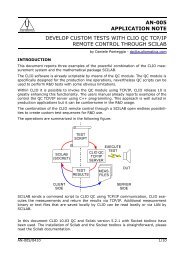
The HR-2000 board will fit in any IBM (or IBM-compatible) Personal Computer and will perform
the A/D and D/A interfacing with the outside world. The board requires a standard 8-bit half-size ISA
slot. The audio connections are made via four RCA plugs; the lower two are outputs, and the upper two
are inputs (see Fig. 2.1). Two adaptor cables with alligator clips are supplied with the board (not in
the Lite version), and can be used to connect to speaker or component terminals when performing
measurements.
INPUT A
INPUT B
OUTPUT A
OUTPUT B
FIGURE 2.1 – The CLIO PC board
2.1.1 TECHNICAL SPECIFICATIONS
GENERATOR
Type:
Two-channel 16-bit sigma-delta D/A converter
Frequency range: 1 Hz–22 kHz (+0/–1 dB)
Frequency accuracy: better than 0.01%
Frequency resolution: 0.01 Hz
Output impedance: 100 ohms
Max. output level (sine): 12 dBu (3.1 Vrms)
Attenuation:
+12 to -64 dBu in 0.1 dB step + mute
THD+Noise (sine): 0.015%
Chapter 2 – The CLIO system 15

ANALYZER
Type:
Input range:
Input impedance:
Phantom:
Two channel 16-bit sigma-delta A/D converter
+30 to –40 dBV
64 kohm
8.2 V (5.6 kohm mic input impedance)
MISCELLANEOUS
Sampling frequencies:
Card type:
Card connections:
51.2 kHz, 25.6 kHz, 12.8 kHz, 6.4 kHz, 3.2 kHz and 1.6 kHz
14 cm, 8-bit PC slot card
Four RCA plugs
Adaptor cables to speaker terminals (not supplied in Lite version)
16 Chapter 2 – The CLIO system

2.2 THE MIC-01 MICROPHONE
The MIC-01 microphone is an electret measuring microphone that is particularly well suited to be used
in conjunction with the other components of the CLIO system. It is furnished with its own stand adaptor
and a calibration chart, all fitted in an elegant case. Its long and thin shape renders it ideal for anechoic
measurements. Because its frequency response is very flat over the entire audio band, no particular
correction is needed for professional-quality measurements.
2.2.1 THE MIC-02 MICROPHONE
The MIC-02 microphone is functionally identical to MIC-01. It differs only in the fact that its length
is 12 cm instead 25 cm. The MIC-02 is more practical to handle and to work with, and is ideal for
measurements in a reverberant environment.
2.2.2 TECHNICAL SPECIFICATIONS
MIC-01
Type:
Accuracy:
Maximum level:
Dimensions:
Accessories:
Condenser electret
±1 dB, 20 Hz to 10 kHz
±2 dB, 10 kHz to 20 kHz (direct field)
130 dB SPL
8 mm diameter, 25 cm long
wooden case, 2.7 m cable, stand adaptor
MIC-02 and Lite
Same as MIC-01, but 12 cm long. In the Lite version the accessories are not supplied.
Chapter 2 – The CLIO system 17

2.3 THE PRE-01 MICROPHONE PREAMPLIFIER
The microphone preamplifier PRE-01 has been designed to match Audiomatica’s microphones MIC-
01 and MIC-02. It is particularly useful when the microphone has to be operated far from the analyzer
or when weighted measurements are needed. PRE-01 powers the microphone connected to its input
with an 8.2V phantom supply and adds a selectable weighting filter (A or B or C); also available there
is a 20 dB gain stage. The unit is operated with two standard 9V batteries or with an external DC power
supply. PRE-01 substitutes the 3381/A preamplifier.
PRE01
AUDIOMATICA
ON
ON
OFF
OFF
INPUT OUTPUT FILTER TEST POWER
2.3.1 TECHNICAL SPECIFICATION
PRE-01 front panel.
Frequency response:
7Hz÷110kHz (-3dB)
Weighting filter: A, B, C (IEC 651 - TYPE I)
Phantom power supply:
8.2V (5600 Ohm)
Gain:
0 & 20dB (INTERNAL SETTINGS)
Input impedance:
5600 Ohm
Output impedance:
100 Ohm
Maximum output voltage (@1kHz):
25 Vpp
THD (@1kHz): 0.01%
Input noise (@20dB gain):
7uV LIN, 5.3uV A
Drive capability:
±7mA
Batteries duration:
>24h (alkaline cells)
Size:
12.5x19x5cm
Weight:
900g
2.3.2 USE OF THE PREAMPLIFIER
The MIC-01 or MIC-02 microphone cable has to be connected to the preamplifier input while the
preamplifier output has to be connected to the analyzer input. The unit is switched on with the POWER
switch, while the TEST push-button controls the state of the unit; when pressing it, if the led light is
on then the unit operates correctly, otherwise not: either the batteries are low or the external power
supply is not connected. The FILTER switch inserts the weigthing filter. To choose the desired
weighting filter type and to set the amplifier gain you have to modify the internal settings as described
later.
NOTE: if the 20 dB gain stage is inserted the overall sensitivity (microphone + pre) is 10 times higher.
For example if your microphone has a sensitivity of 17.1 mV/Pa and you preamplify it of 20 dB then
you get a sensitivity of 171 mV/Pa.
18 Chapter 2 – The CLIO system

2.4 THE CLIOQC AMPLIFIER & SWITCH BOX
The CLIOQC amplifier and switch box is of invaluable help when configuring an automatic or manual
quality control setup and even in everyday laboratory use.
Its main feature is the possibility of internal switching that permits the measurement of the impedance
and frequency response of the loudspeaker connected to its output sockets without changing the
loudpeaker wiring; it is also possible to choose one among several input for the respoonse
measurements; the internal switching is under software control via the parallel port of the PC. The two
models (Model 2 and 3) differ for the number of available inputs: 2 or 8.
INPUT
FROM CLIO
1
D.U.T.
TO CLIO
CLIOQC
2 ampli&switchbox
AUDIOMATICA
I SENSE
Model 2 front panel
INPUT
FROM CLIO
1
3
5
7
D.U.T.
TO CLIO
CLIOQC
2 4 6 8
ampli&switchbox
AUDIOMATICA
I SENSE
Follows its internal block diagram.
Model 3 front panel
PC control
Input 1
Input 2
To CLIO
Input 8
Speaker
10 dB
From CLIO
I Sense
Internal connections for frequency response measurements
Chapter 2 – The CLIO system 19

PC control
Input 1
Input 2
To CLIO
Input 8
Speaker
10 dB
From CLIO
I Sense
Internal connections for impedance measurements
2.4.1 TECHNICAL SPECIFICATIONS
Inputs:
Two (Model 2) or eight (Model 3) line/microphone inputs with
selectable phantom power supply (8.2V)
Functions:
TTL controlled internal switches for impedance measurements
Output power: 10W with current sensing
THD (1 kHz): 0.004 %
Dimensions (cm): 23x9x23
Weight:
2.7 kg
AC: 110-120/220-240
20 Chapter 2 – The CLIO system

3 INSTALLATION OF CLIO
NOTE: PLEASE REFER TO CHAPTER 4 FOR POTENTIAL PROBLEMS REGARDING THE
COMPATIBILITY OF THE CLIO SYSTEM WITH YOUR PC (EITHER HARDWARE OR
SOFTWARE).
3.1 PC CONFIGURATION
The CLIO PC board running the system software version 4 Standard, Lite or QC can be fitted in any
IBM (or compatible) personal computer with the following minimum system requirements:
– 486 processor (suggested minimum DX-33)
– one free 8-bit or 16-bit half-size ISA slot
– 2 MB RAM
– hard disk
– VGA video board
– MS-DOS Version 3.2 or later
A math co-processor is not required but is highly recommended.
3.2 HARDWARE INSTALLATION
It is possible to configure the I/O address of the CLIO board, by means of the JP2 jumper, in order to
avoid conflicts with other boards that are installed in your computer. Refer to Fig.3.1 where you can
see the two possible positions of JP2. The I/O space used by CLIO is four bytes wide, and starts at the
base address that has been selected (i.e. 300-303 HEX if the 300 HEX choice has been made).
FIGURE 3.1a – I/O address 300 HEX
FIGURE 3.1b – I/O address 310 HEX
The situation depicted in Fig.3.1a is the factory default.
For any further problem regarding the jumper settings refer to paragraph 7.3.3. Jumper JP1 has no effect
either on the installation or the current software functionality; it has to be left as factory shipped.
To install the CLIO board in your computer you should follow the instructions presented below:
1) Disconnect the mains power cable from the PC.
2) Open the computer cabinet.
3) With the motherboard in front of you, identify a free 8-bit (or 16-bit) slot. Note that it is preferable
to install the CLIO board as far away as possible from the video adaptor.
4) Insert the CLIO board in the slot and screw it down firmly.
Chapter 3 – Installation 21

5) Close the cabinet.
6) Reconnect the mains cable and switch the computer on.
At this point the CLIO board hardware installation is finished. To proceed further, you need an RCA
pin-to-pin cable (one of those used in a stereo system) to connect the CLIO channel A input and channel
A output; we strongly suggest you to carefully follow paragraph 3.4 in order to verify the correct
behavior of your CLIO system.
You should always keep in mind the following electrical specifications of your CLIO system:
MAXIMUM INPUT VOLTAGE:
MAXIMUM OUTPUT VOLTAGE:
INPUT IMPEDANCE:
OUTPUT IMPEDANCE:
+30 dBV (89.5 V peak-to-peak)
+12 dBu (3.1 Vrms) (sine)
64 kohm
100 ohm
3.3 SOFTWARE INSTALLATION
The CLIO software is provided on a 3.5" (1.44 MB) diskette named “PROGRAM DISK”.
The software has to be installed on the hard disk of your PC. The installation procedure is carried out
by running the INSTALL.BAT batch file that is supplied on the program disk. This will create a CLIOxx
directory with two subdirectories, one called DATA and the other called SIGNAL. “xx” denotes the
software version number. For this edition the actual version number is 4.0, so a CLIO40 directory will
be created.
To install the CLIO software do the following:
1) Insert the “PROGRAM DISK” in your PC.
2) Type the following command (from DOS prompt or W95/98 Start button and then Run option):
{source drive}INSTALL {optional source drive}{optional destination drive}
where {drive} is, for example, A: or D: and indicates that you should press the Enter key
on your keyboard.
As an example “B: INSTALL B: D:” installs CLIO from drive B: to drive D:; if you only specify
“INSTALL” without arguments CLIO will assume A: source drive and C: destination drive.
The DOS PATH should not contain the C:\CLIO40 path; CLIO has not to be run from outside the CLIO40
directory! CLIO requires at least 580K of conventional memory; use the appropriate DOS command
to check this requirement before running CLIO.
Now you will run CLIO for the first time; please follow carefully the procedure described in the
following chapter: verify that you obtain EXACTLY what is described in the manual and DO NOT
proceed to the subsequent step if you where not able to complete the previous successfully.
As an example NEVER PERFORM A CALIBRATION if you were not able to play a sinusoid:
THERE IS A PROBLEM THAT HAS TO BE SOLVED !
When contacting technical support report what has happened and where your verification
procedure stopped.
22 Chapter 3 – Installation

3.4 RUNNING CLIO FOR THE FIRST TIME
If you have completed the preceding installation procedure,
you are ready to run CLIO!
The steps hereafter described will guide you through a
complete verification of the system performance and
operation.
FIGURE 3.2
To run the software just type CLIO (be sure to start from within
the CLIO system directory) and . You should see
CLIO’s main window (Fig. 3.2). After having answered the
initial prompt you are ready to make your first measurement.
Should there be any problem with the installation the program
will display a warning message. In the event that a warning
message does occur, please refer to Chapter 7 to properly
setup your board.
FIGURE 3.3
FIGURE 3.4
FIGURE 3.5
The board has to be connected as depicted in Fig. 3.14 (with
input A and output A short-circuited); do not change this
connection throughout all the tests described in this section.
Let’s now start with a simple level measurement of a 1000 Hz
sinusoid generated by CLIO: press F4 to recall the Generator
and Level Meter control panel and then “S” or click on the Sin
button to start the definition of a sinusoidal signal; type in 1000
in the Freq field (leave the other fields at 0) and press Enter
or click on the Ok button (as shown in Fig. 3.3); the generator
display will show “1000 SIN” and the level meter will
measure about “0.77 V” which is the default output level of a
sinusoidal signal (as shown in Fig. 3.4).
Now you are ready to view the signal with the Oscilloscope;
press Esc or click on the “X” title bar button to exit the
Generator control panel and then press “T” and “S” for the
Tools Scope option; once in the Oscilloscope control panel
you may press “G” to start the interactive oscilloscope; using
the UP-ARROW and DOWN-ARROW keys you can freely
change the vertical amplification of the acquired waveform
and pressing “F” you are able to freeze it and view a stable
screen (Fig. 3.5). Press Esc to exit the oscilloscope.
FIGURE 3.6
If you're running a Lite software version, please skip the
following lines and go directly to the description of system
calibration. Now we are ready for a frequency measurement:
press “F” to invoke the FFT analyzer; pressing “S” begins the
FFT analysis; as in the oscilloscope case the measurement is
continuously refreshing and pressing “T” stops the acquisition:
the single line that you see is the spectral content of the
generated sinusoid (Fig. 3.6); using the LEFT-ARROW and
RIGHT-ARROW keys or moving the marker with the mouse
Chapter 3 – Installation 23

you can inspect the amplitude of each single frequency bin,
if it is positioned as in figure the marker will read the level
at 1 kHz of -2.2 dBV. Press Esc to exit the FFT control panel
and go back to CLIO’s main menu.
FIGURE 3.7
FIGURE 3.8
FIGURE 3.9
FIGURE 3.10
We will now undertake the system calibration procedure:
press “D” to enter the Disk menu and “C” to start the system
calibration (Fig. 3.7); press Enter to start the procedure;
please be patient as this procedure will take some minutes;
you will see several progress indicators that will accompany
each calibration performed; as the procedure ends you will
have control of the system again and are ready for an MLS
check.
Press “M” and then “A” to invoke the MLS Analysis control
panel; now press “G” to run your first MLS measurement,
after some seconds the computer will play a short beep and
you should see, on your screen, a straight line as in Fig.3.8;
this means that your system is correctly calibrated with
respect to the amplitude of the MLS frequency response;
press now “P” to get the phase plot and you should obtain
another straigth line as in Fig.3.9; this means that your system
is correctly calibrated with respect to the phase of the MLS
frequency response.
NOTE: the average amplitude reading of the marker is -5.1
dBV (the default output level of the MLS signal file).
Press Esc to exit the MLS control panel and go back to the
main menu. Press “S” and then “F” to invoke the Sinusoidal
Frequency Response control panel; now press “G” to run
your first Sinusoidal measurement, for several seconds the
computer will play a sinusoidal sweep from 10 Hz to 20 kHz;
you will see the frequency played on the status line in the
bottom of the screen; at the end of the process you should see
a straight line as in Fig.3.10; this means that your system is
correctly calibrated with respect to the amplitude of the
Sinusoidal frequency response; press now “P” to get the
phase plot and you should obtain another straigth line as in
Fig.3.11; this means that your system is correctly calibrated
with respect to the phase of the Sinusoidal frequency response.
NOTE: the average amplitude reading of the marker is -2.2
dBV (the default output level of a sinusoidal signal, as seen
before).
If you completed succesfully this hard job your system
should perform correctly and you are ready to get the
most satisfactory results from your CLIO.
FIGURE 3.11
24 Chapter 3 – Installation

To start working with CLIO you may want to familiarize yourself with the user interface and the many
hot keys. Read carefully chapters “5-Clio’s User Interface”, “6-Disk Menu and Files management” and
“7-Configuring and Calibrating Clio” after this chapter before proceeding further.
3.5 CLIO CONNECTIONS
The CLIO board has four RCA plugs that are used to connect it with the outside world (Fig. 3.12). The
lower ones, J1 and J2, are the two outputs, while J3 and J4 are the inputs. The board is stereo and can
simultaneously process two I/O channels which are named channel A and B. The output of channel B
is normally driven in parallel with channel A output but can be separately muted.
INPUT A
INPUT B
OUTPUT A
OUTPUT B
FIGURE 3.12 – The CLIO PC board
The software is able to analyze either the signal present at channel A or channel B input in an unbalanced
configuration or the combined A-B signal thus realizing a balanced input configuration (Fig. 3.13); in
the first case the input connection can be realized with one simple RCA cable while in the latter case
it is mandatory to realize a balanced probe that will connect channel A input (used as the positive or
“hot”) to the first measuring point, channel B input (used as the negative or “cold”) to the second
INPUT A
+
PC-IBM CLIO
INPUT B
OUTPUT A
G
OUTPUT B
FIGURE 3.13 – Input connection for balanced measurements
Chapter 3 – Installation 25

measuring point and ground. Use Shift-F1 to recall the global/local settings dialog box and select the
input channel desired; refer to chapter 7 for any further detail about it.
WARNING: Both CLIO inputs and outputs are referred to a common measuring ground. When you
are making measurements in the normal configuration (channel A or B unbalanced), one of the two
measuring points MUST be at ground potential! Problems may arise if one tries to use amplifiers with
floating outputs; the connection with CLIO could cause damage to such an amplifier. Use the channel
A-B balanced connection in such cases.
Unless you are executing impedance measurements with the Internal Mode selected (see Chapter 11),
one of CLIO outputs will usually be connected to an external power amplifier that will drive the
loudspeaker, electronic apparatus, or other system under test.
The output of the system under test will be connected to one of the CLIO inputs. For acoustical
measurements, it will be the microphone (optionally followed by a preamplifier) that is connected to
the input channel.
When using the microphone directly connected to CLIO, always remember to switch the phantom
voltage on. It is good practice to wait a few minutes before starting measurements.
If the measuring point is far from the PC, always lengthen the connection between the preamplifier and
CLIO. Make sure that you never use microphone cable that is longer than the one that has been supplied.
In the following set of figures one will find four possible measuring conditions and the relative
connections.
In Fig. 3.14 we see the connection to be used for the calibration procedures. It is necessary to short
circuit the input and output of channel A with a pin-to-pin cable.
In Fig. 3.15 we see the typical test setup for performing acoustical measurements of a loudspeaker.
Please note this schematic diagram, drawn in the assumption of using one Audiomatica microphone
MIC-01 or 02 directly connected to CLIO input, where the output of the power amplifier is connected
to the loudspeaker with an inversion in cables polarity; this compensates the fact that Audiomatica
microphones are phase inverting as almost the vast majority of measuring microphones found in the
market; when making polarity measurements always cure the measuring chain in this respect
considering that the CLIO board itself is NON-INVERTING and that all calibrations are usually made
under this assumption: any external device like amplifiers, microphones, accelerometers, preamplifiers
etc. has to be carefully checked.
In Fig. 3.16 we see the connection that is used to make impedance measurements or to measure the
Thiele-Small parameters of a loudspeaker driver. When using the Internal Mode the connection is
normally realized using the supplied adaptor cables (pin to alligators). Refer to Chapter 11 for any
further detail on impedance measurements.
A case of particular interest is when the CLIOQC Amplifier & Switch Box is used (Fig. 3.17 and 3.18
where the Model 3 unit is showed).
26 Chapter 3 – Installation

PC-IBM
CLIO
INPUT A
INPUT B
OUTPUT A
OUTPUT B
FIGURE 3.14 – Connection for calibration
PC-IBM
CLIO
INPUT (A OR B)
OUTPUT (A OR B)
MIC-01 OR 02
AMPLI
BLA CK
RED
RED
BLA CK
FIGURE 3.15 – Connection for loudspeaker sound pressure measurements (see text)
Chapter 3 – Installation 27

INPUT A
PC-IBM CLIO
INPUT B
OUTPUT A
Z X
OUTPUT B
FIGURE 3.16a – Impedance measurements in "Internal Mode"
INPUT A
PC-IBM
CLIO
INPUT B
OUTPUT A
R S
OUTPUT B
Z X
BLA CK
AMPLI
RED
FIGURE 3.16b – Impedance measurements with an external sensing resistor Rs in "Constant Current Mode"
INPUT A
PC-IBM CLIO
INPUT B
OUTPUT A
Z X
OUTPUT B
R S
BLA CK
AMPLI
RED
FIGURE 3.16c – Impedance measurements with an external sensing resistor Rs in "Constant Voltage Mode"
FIGURE 3.16 – Connection for impedance measurements
28 Chapter 3 – Installation

PC-IBM
CLIO
INPUT A
INPUT B
OUTPUT A
OUTPUT B
LPT PORT
CLIOQC AMPLIFIER&SWITCHBOX
I SENSE
BLACK
RED
10 dB
FROM CLIO
INPUT 1
INPUT 2
TO CLIO
INPUT 8
FIGURE 3.17 – ClioQC Ampli&SwitchBox with internal connection for response measurements
INPUT A
PC-IBM
CLIO
INPUT B
OUTPUT A
OUTPUT B
LPT PORT
CLIOQC AMPLIFIER&SWITCHBOX
I SENSE
BLACK
RED
10 dB
FROM CLIO
INPUT 1
INPUT 2
TO CLIO
INPUT 8
FIGURE 3.18 – ClioQC Ampli&SwitchBox with internal connection for impedance measurements
Chapter 3 – Installation 29

30 Chapter 3 – Installation

4 PC COMPATIBILITY
4.1 HARDWARE COMPATIBILITY
CLIO’s hardware makes intensive use of the resources of the computer in which it is installed. Its
functionality is based on two DMA (Direct Memory Access) 8-bit channels that are present on the PC
main board with 80286 and higher processors. One DMA channel is used for generation and the other
for acquisition. Four I/O addresses are also used, and these can be specified to start at HEX 300 or
HEX 310, depending on board and software configurations.
DMA channels number 1 and number 3 are used.
As a result, it is possible that the CLIO board might not be compatible with any other board using the
same DMA channels, at least, but not only, in multitasking operating system environments (eg. Microsoft
Windows). The CLIO board is not compatible with any other board that uses the same I/O addresses.
You should always check these items before proceeding with CLIO installation.
4.2 SOFTWARE COMPATIBILITY
CLIO software release 4 is a DOS native application; it can be run under Windows 95/98 and we suggest
you to use CLIO in a DOS window; in our experience it is not mandatory to run CLIO in MS-DOS
exclusive mode shutting down Windows; all the limitations common to DOS program running under
those environments apply.
As already stated, CLIO fully utilizes the computer’s resources. Aside from memory requirements, it
is also good practice to avoid using CLIO when other memory resident programs are installed, aside
from the mouse driver, without having previously made extensive test. This is because it is not possible
to verify that these memory resident programs will have no adverse affects on the functionality of CLIO
without having tried each program in turn.
We strongly suggest that you start with the PC system in its simplest possible configuration. After that,
every time you add a memory resident program, always check to ensure that CLIO has not lost time
control of generation/acquisition. This can be easily verified with a phase measurement performed with
the input and output of the board connected as suggested in the calibration procedure.
Chapter 4 – PC compatibility 31

32 Chapter 4 – PC compatibility

5 CLIO’S USER INTERFACE
5.1 GENERAL INFORMATION
CLIO’s user interface has been created by embodying many modern concepts relating to the design of
graphical user interfaces for programs running on personal computers. Many of these ideas have been
implemented in products such as the Microsoft Windows graphical environment, which has enjoyed
a high degree of acceptance by computer users. With such a philosophy as an inspiration, which today
is a commonly recognized standard, the CLIO program should be easy for the user to comprehend and
operate.
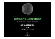
Fig. 5.1 shows CLIO’s initial screen. Aside from normal graphical user interface objects such as menus,
scroll bars, dialog boxes, radio buttons, etc., CLIO’s user interface furnishes a comfortable work area
via a control panel. This has been developed to make the PC screen as similar as possible to a traditional
instrument (see section 5.3), and the contents of each control panel will change depending on the
particular task that is to be carried out.
Let us now move on to describe in detail the most important user interface objects that one will meet
when working with CLIO.
5.2 MENUS
FIGURE 5.1 – CLIO's startup screen and user interface
Menus allow a number of operational choices to be gathered into specific
subject categories. They are structured in a hierarchical “upside-down
tree” manner (as are the directories of a disk). CLIO’s main window,
which is a menu in itself, is at the highest level (equivalent to the root
directory of a disk).
Choices may be made by either positioning the mouse or by entering the
underlined letter by means of the keyboard, or by moving the highlighted
bar with the arrow keys and making the selection with the Enter key.
FIGURE 5.2
It is possible to exit from all menus by simply pressing the Esc key.
Chapter 5 – CLIO’s User Interface 33

5.3 CONTROL PANELS
Fig. 5.3 shows a typical control panel (obtained after choosing the Analyze option from the MLS menu).
In general, the screen will be divided into three physically and functionally distinct areas.
title bar buttons
cursor
title bar
measurement screen
status line
FIGURE 5.3 – A typical control panel
function buttons
Within the graphical window, whose title gives the name of the control panel, the following regions
are present:
THE MEASUREMENT SCREEN
This represents the screen of a traditional instrument, and it occupies the major part of the window and
presents the results obtained from the measurement that was executed.
NOTE: It is normally possible to check results of a measurement through the use of an on-screen cursor.
This can be directly activated with the mouse (dragging is possible by keeping the left button pressed).
The numerical values associated with a given point on the graphical plot will usually be written on the
status line (see above).
FUNCTION BUTTONS
These are found immediately under the measurement screen, and they represent the buttons that might
normally be present on the instrument’s panel. Each button has a label that serves to describe its function.
By selecting these buttons, it is possible to execute the measurement and check parameters.
These function buttons may be “pressed” by positioning the mouse pointer on top of the selected function
button and then clicking the left mouse button. It is also possible to make a selection by pressing the
key on your keyboard that corresponds to the underlined letter on the button label.
There are two different kinds of buttons. The most common one immediately returns to the starting
position after being pressed, and this kind of button serves to confirm an action. The other type of button
34 Chapter 5 – CLIO’s User Interface

emains active when it is pressed, and changes colour to confirm that a particular operational mode
has been selected. To deactivate such buttons it necessary to press them a second time.
THE STATUS LINE
This is located between the function buttons and the end of the graphics window, and it is used to present
useful messages to the user that help to enhance the understanding of the measurement. For example,
these status messages include such things as the file name, the input overload status, the cursor’s
position, as well as many others.
THE TITLE BAR BUTTONS
Loads a measurement and activates the Load menu option. See section 6.3.
Equivalent to the F2 Hot Key.
Saves the measurement on disk and activates the Save menu option. See section 6.4.
Equivalent to the F3 Hot Key.
Prints the executed measurement.
Equivalent to the Alt-P Hot Key.
Recalls the local Help On Line.
Equivalent to the Ctrl-F1 Hot Key.
Exits the current control panel or dialog box.
Equivalent to the Esc Hot Key.
Chapter 5 – CLIO’s User Interface 35

5.4 HOT KEYS
These are the keyboard keys that are always active from within any menu or control panel. They are
a quick and convenient way to execute many of the most commonly used operations. They are not visible
and therefore may not be selected with the mouse. After frequent use, these keys should become easy
to remember. Let us now take a look at them in detail:
ESC
Alt-P
F1
Exits the current control panel or dialog box.
Prints the executed measurements from within any control panel. To select the print
options refer to Chapter 7.
Turns off any active generation and is the quickest way to kill the generator.
SHIFT-F1 Enters the Measurement Setting dialog box. See Chapter 7.
CTRL-F1
Recalls the local Help On Line. See later.
F2 Saves the measurement on disk and activates the Save menu option. See section 6.4.
SHIFT-F2 Exports the measurement as an ASCII data file. See Chapter 13.
F3 Loads a measurement and activates the Load menu option. See section 6.3.
SHIFT-F3
Imports the measurement from an ASCII data file (only Sinusoidal Frequency Response).
F4 Activates the Generator & Level Meter control panel. See Chapter 8.
SHIFT-F4
Recalls the CLIOQC Ampli & SwitchBox controls (Only if a parallel port has been
selected with the TTL CONTROL radio button). See section 7.4.4.
F5 Used to change the working directory; activates the Chdir menu option. See section 6.6.
F6 Creates a new directory on disk; activates the Mkdir menu option. See section 6.5.
F7 Decrements the output signal level in 1.0 dB steps. See section 8.1.5.
SHIFT-F7 Decrements the output signal level in 0.1 dB steps. See section 8.1.5.
F8 Increments the output signal level in 1.0 dB steps. See section 8.1.5.
SHIFT-F8 Increments the output signal level in 0.1 dB steps. See section 8.1.5.
F9 Decrements the input sensitivity in 10 dB steps. See section 8.1.4.
F10 Increments the input sensitivity in 10 dB steps. See section 8.1.4.
↑
↓
Shifts the displayed curve upwards (according to the current range of the amplitude
display).
Shifts the displayed curve downwards (according to the current range of the amplitude
display).
36 Chapter 5 – CLIO’s User Interface

5.5 CLIO HELP ON LINE
Pressing the Ctrl-F1 Hot Key or clicking on the icon you enter the CLIO Help On Line (Fig. 5.4).
FIGURE 5.4 – CLIO Help On Line (from MLS control panel)
This dialog box gives help relative to the control panel from which it has been recalled; to navigate
it is possible to use the ↑, ↓, PageUp, PageDown, Home and End keys.
Chapter 5 – CLIO’s User Interface 37

38 Chapter 5 – CLIO’s User Interface

6 DISK MENU AND FILES MANAGEMENT
6.1 INTRODUCTION
As you might expect from its title, this chapter deals with the functions that result in read or write access
to and from the hard disk. Setup, Calibration and Exit functions, although not logically tied to disk
operations, are also present in this menu as they are of such common use.
Before we begin examining each item on this menu, we strongly recommend that you read through the
chapter 5 describing the use of CLIO’s “hot keys”. Amongst other things, the hot keys allow the Load
and Save commands to be quickly accessed from every other menu in the program.
6.2 DATA FILES ORGANISATION
The CLIO program is organised in a rather rigid structure on the hard disk, and this does not allow the
user to wander around the directories. Data files containing measurements obtained by the user are
gathered under the DATA subdirectory (which must in all cases be named as such), and under further
subdirectories which the user may define whose prototype is the JOB1 directory (also obligatory). The
JOB1 subdirectory is automatically created by the installation program.
CLIOxx DATA JOB1
USER1
...........
...........
USERn
At the same level as that of the JOB1 directory, other directories may be created from within CLIO by
means of the Mkdir menu option found under the Disk command on the main menu bar. After a new
directory has been created it may be made current through the Chdir menu option. All data files will
be loaded or saved within the current directory.
Last but not least, it is not possible to remove any kind of file and load or save files on floppy disks
from within the program.
6.3 LOADING FILES
Loading a file is performed either as a startup option to configure your CLIO working environment
(see 7.2) or from within each measurement control panel pressing the dedicated hot key or clicking
on the appropriate title bar button (see 5.3 and 5.4).
When you are inside a control panel you may press F3 or click on the “LOAD” icon; the Load
FIGURE 6.1 – The Load File dialog box
Chapter 6 – Disk Menu and files management 39

File dialog box appears as in Fig. 6.1 (as an example from the MLS Analyze control panel). This dialog
box displays a list of files all of which have the same extension used in that prticular control panel.
As a refernece the file name extensions that CLIO uses are:
Fft:
measurement files obtained through the Fft menu.
Mls: measurement files obtained through the MLS Analyze menu.
Wtf: measurement files obtained through the Mls Waterfall menu.
Frs: measurement files obtained through the Sinusoidal Frequency Response menu.
Imp: measurement files obtained through the Sinusoidal Impedance menu.
Sml: measurement files obtained through the Sinusoidal Parameters menu.
Dst: measurement files obtained through the Sinusoidal Distortion menu.
Pol: measurement files obtained through the Sinusoidal Polar menu.
Rta: measurement files obtained through the RTA menu.
T60: measurement files obtained through the Acoustics RT60 menu.
Leq: measurement files obtained through the Acoustics Leq menu.
Spe: measurement files obtained through the Tools Scope menu.
To load the desired file, select it by using either the arrow keys on the keyboard or the mouse. Then
either click the Load button, press the underlined letter L, or give a double-click with the mouse on the
selected file name in the file list. It is possible to load, in sequence, files of all types, and these will
be plotted once the related control panel has been accessed.
6.4 SAVING FILES
When you are inside a control panel, and some measurement data are present in memory, you may
press F2 or click on the “SAVE” icon to recall the Save File window (Fig. 6.2).
FIGURE 6.2 – The Save File dialog box
The mode of operation is the same as that described for the Load File window. As might be expected,
the filename extensions are also the same. You will automatically be prompted for the name of the file
to be saved.
Should there already be a file with the same name and extension, you will be asked to confirm the save
40 Chapter 6 – Disk Menu and files management

operation. The directory in which the file is saved is the current active directory (see the Chdir and
Mkdir menu commands for further details). Aside from the measurement itself, additional relevant
information will also be saved. This includes a comment that can be added by means of the About button,
as well as several settings related to the measurement.
6.5 Mkdir
This command creates new work subdirectories that will be put under the DATA directory. All new
directories are at the same level as the JOB1 directory which is created by the installation program.
Therefore, it is possible to place sets of measurements into different subdirectories. When the CLIO
program is first loaded, the default directory where measurements and files of all extensions are saved
is JOB1. The same effect may be obtained, when you are inside a control panel, pressing the F6 Hot
Key.
6.6 Chdir
This command is used to change the current directory where all measurements and files with different
extensions will be saved to or loaded from. In order to be able to change to a particular directory, it
must of course exist, and it will usually have been created using the Mkdir command. The same effect
may be obtained, when you are inside a control panel, pressing the F5 Hot Key.
When exiting from CLIO, the current directory will be saved in the CLIO.STP file. When the CLIO
program is re-loaded, the last selected directory will be automatically selected.
6.7 Setup
Refer to Section 7.4 “THE DISK Setup CHOICE” for a detailed explanation of this choice.
6.8 Calibration
Refer to Section 7.6 “CALIBRATING CLIO” for a detailed explanation of this choice.
6.8 Exit
This command ends the CLIO work session.
Chapter 6 – Disk Menu and files management 41

42 Chapter 6 – Disk Menu and files management

7 CONFIGURING AND CALIBRATING CLIO
7.1 INTRODUCTION
This chapter explains how to correctly configure the CLIO system software in order to obtain the best
results when performing electrical and acoustical measurements. Section 7.2 will explain how to
configure CLIO at startup. Section 7.3 will deal with some software configuration issues related to the
CLIO board that will affect all measurements. Section 7.4 will cover various aspects of configuration
that are related to the PC platform (e.g. printer devices) and are usually found in all software products.
Section 7.6 will explain how and when to calibrate the system.
7.2 SOFTWARE STARTUP OPTIONS
It is possible to run the CLIO software using the following syntax:
“CLIO {menu} [opt. {work directory}] [opt. {file}] “
The three parameters permit the user to directly access a measurement menu, select an optional work
directory and load a previously saved file; they are defined as:
{menu}
A three letter acronym to specify the relative menu:
FFT FFT
MLS MLS Analyze
WTF MLS Waterfall
FRS Sinusoidal Frequency Response
IMP Sinusoidal Impedance
SML Sinusoidal Parameters
DST Sinusoidal Distortion
POL Sinusoidal Polar
RTA RTA Analyze
T60 T60
LEQ Leq
SPE Oscilloscope
QC QC
{work dir.} A work directory already present under DATA\.
{file}
A measurement file already saved on disk; it has to be specified with the correct extension.
As an example the following:
“CLIO MLS JOB1 SAMPLE.MLS”
will directly enter the MLS Analyze menu, select the JOB1 directory as the active one and load the
SAMPLE.MLS file.
NOTE: All the measurement settings saved with the file are recalled and affect any measurement that
will be executed after.
Chapter 7 – Configuring and calibrating CLIO 43

7.3 MEASUREMENT SETTINGS
The measurement specific configuration items can be input from within some control panels or even
from the main window. There are Local Measurement Settings that are private to each type of
measurement and are loaded every time one enters a control panel. There are also the Global
Measurement Settings that are the default condition when the program is run for the first time, and
these settings are subsequently saved in the CLIO.STP file (see section 7.4).
NOTE: Each time the program is run, all Local Measurement Settings are initialized to the Global
Measurement Settings. During a work session one can freely change the Local Settings so that they will
differ from each other and from the Global Settings. A common event that changes the Local Settings
is when a measurement is loaded from disk: the Local Settings are also loaded from disk to match those
of the loaded measurement.
The Measurement Settings can be changed from within the dialog box shown in Fig. 7.1. The
measurements that are affected by these settings are: FFT, MLS, Sinusoidal Frequency Response,
Sinusoidal Polar, RTA, Leq, Scope and the Generator & Level Meter. This dialog box can be recalled
from within the various control panels (with the exception of Scope), by pressing the SHIFT-F1 hotkey
or with the Sett button in the Generator & Level Meter control panel (see section 8.1).
FIGURE 7.1 – The Measurement Settings dialog box
7.3.1 INPUT CHANNEL
It is possible to select the input channel for analysis. There are three possibilities:
CH A
CH B
CH A-B
Channel A used as input in an unbalanced configuration.
Channel B used as input in an unbalanced configuration.
Both channels are used as input in a balanced configuration.
Please refer to paragraph 3.5 for details on the input connections to be realized in each situation.
7.3.2 SAMPLING FREQUENCY
It is possible to select one of three possible sampling frequencies: 51200 Hz, 12800 Hz, and 3200 Hz.
This selection will take effect only in the following measurements:
– Generator & Level Meter
– FFT
44 Chapter 7 – Configuring and calibrating CLIO

– MLS
– Scope
NOTE: The lower the sampling frequency that you choose, the slower will become some of the
measurements. This fact is readily understood if one considers the theory behind the sampling process.
For example, if executed using a 3200 Hz sampling rate, the MLS measurement will take about 16 times
the length of time it takes if executed at 51200 Hz (in fact the generator needs exactly 16 times the time
to play the MLS of the same length).
7.3.3 PRESSURE MODE AND MICROPHONE CORRECTION
It is possible to select the Pressure measuring mode. When not in Pressure mode, the readings displayed
by the instrument and the amplitude scales on all the graphs will be in Volts (Vrms or dBV). When in
Pressure mode, the readings and the scales will be in Pascals (Pa or dB SPL). In this case, the software
will assume that you are measuring a pressure quantity and it therefore needs to know a conversion factor
that defines the voltage produced by the microphone when it is measuring a certain pressure. This
conversion factor is usually the sensitivity of the microphone (as found in the microphone’s calibration
chart) or the sensitivity of the microphone + preamplifier chain of equipment. When working with the
CLIO system there are two possible cases:
a) you are using the microphone MIC-01 or MIC-02, so it is necessary to input the sensitivity of the
microphone (in mV/Pa).
b) you are using the 3381/A preamplifier, so it is necessary to input the value of the scale selected
on the preamplifier (in dB SPL/V).
NOTE: It is necessary to input two separate sensitivities, one for channel A and one for channel B. When
it is selected the A-B balanced input configuration the software will use the channel A sensitivity.
It is also possible to activate, in Pressure mode, the Microphone Correction check box; if activated
the software will correct the measured curve according to the data stored in the “MIC.CAL” file. The
example below shows a sample text file created to store the microphone frequency response:
Freq dB Phase
1000 0 0
4000 0.25 0
8000 0.33 0
10000 0.5 0
15000 1.75 0
20000 2.5 0
NOTE: This correction will take effect in the MLS Analyze, Sinusoidal Frequency Response and RTA
control panels. Always remember that the measurement data, stored in all CLIO files, are NOT
corrected by the microphone file data.
NOTE: When working with the preamplifier, take care that CLIO’s input gain is never set below –10
dBV; this prevents the possibility of overloading the preamplifier without having any status message
displayed.
7.3.4 THE Globals BUTTON
This is a quick way to reset the Local Measurement Settings to the actual Global Measurement Settings.
Chapter 7 – Configuring and calibrating CLIO 45

7.4 THE DISK Setup CHOICE
After choosing Setup from within the Disk command presented on the menu bar, one enters the Setup
dialog box, which is shown in Fig.7.2. It is possible to configure your printer, on-screen colours, as
well as CLIO’s I/O address from the various parameters displayed in this dialog box.
7.4.1 PRINTERS
FIGURE 7.2 – The Disk Setup dialog box
It is possible to select one of three popular printer families: Hewlett-Packard (HP), Epson, and IBM;
otherwise the printout can be redirected to a standard Windows “.BMP” black-and-white bitmap file.
It is also possible to select the output printer port (LPT1 or LPT2) and set an option via a check box
to send a form-feed command after each measurement is printed.
7.4.2 COLOURS
This option lets the user select from one of seven different colour choices.
NOTE: Palettes 6 and 7 have been developed for use with monochrome displays.
7.4.3 I/O ADDRESS
The CLIO system software automatically detects the board I/O address at startup. It is nevertheless
possible to configure the I/O address of the CLIO board in order to avoid conflicts with other boards
that are installed in your computer. Refer to Fig.7.3 where you can see the two possible positions of
JP2. The I/O space used by CLIO is four bytes wide, and starts at the base address that has been selected
(i.e. 300-303 HEX if the 300 HEX choice has been made).
The situation depicted in Fig. 7.3a is the factory default.
FIGURE 7.3a – I/O address 300 HEX
FIGURE 7.3b – I/O address 310 HEX
46 Chapter 7 – Configuring and calibrating CLIO

7.4.4 EXTERNAL HARDWARE CONTROL
The CLIO software release 4 and QC is able to control external hardware by means of the TTL signals
generated with the parallel printer port of the PC. It is possible to activate the selected printer port for
external control or disable it. If TTLCONTROL is left to OFF no output control is performed (also
the SHIFT-F4 hot key is disabled). Actually we have three possibilities:
1) The control of CLIOQC Amplifier & Switch Box
First select the model of the CLIOQC Ampli&SwitchBox with the "AMPLI&SWITCH" radio button.
After you have connected the unit to the PC printer port it is possible to control its internal switches
simply pressing SHIFT-F4; one of the following dialog boxes appear:
It is straightforward to understand its functionality; refer also to figure 3.17 when selecting one of the
input for a response measurement and to figure 3.18 when selecting the impedance connection.
NOTE: This dialog box is active only if a printer port is selected; if the TTL CONTROL radio button
is OFF then no dialog box appears when SHIFT-F4 is pressed.
2) The control of the Outline ET1/ST1 Turntable
When making polar measurements (see paragraph
11.6) CLIO is able to directly control the OUTLINE
ET1/ST1 Turntable by means of BIT 7 of the selected
parallel printer port (see figure right).
3) The control of an external automation in a QC
production line
During a Quality Control test setup it is possible to
integrate CLIO in a line automation (see chapter 15);
the QC measurement can control up to eight different
signals to reflect the result of an executed test and can
also be externally triggered in order to realize a fully
automated environment.
1
14
2
15
3
16
4
17
5
18
6
19
7
20
8
21
9
22
10
23
11
24
12
25
13
BIT 0
BIT 1
BIT 2
BIT 3
BIT 4
BIT 5
BIT 6
BIT 7
START
OUTLINE ET1/ST1
CONTROL
7.5 THE SETUP FILE
All the above mentioned software configuration items are saved in a setup file called CLIO.STP that
is saved in the main CLIO directory. This file will be loaded automatically every time CLIO is started,
thus re-configuring it to the last used state.
NOTE: If, for any reason, you want to return to a known default condition, you can delete the CLIO.STP
file. This will cause the CLIO software to load a built-in default configuration.
Chapter 7 – Configuring and calibrating CLIO 47

7.6 CALIBRATING CLIO
To calibrate CLIO it is necessary to connect the A output directly to the A input.
PC-IBM
CLIO
INPUT A
INPUT B
OUTPUT A
OUTPUT B
FIGURE 7.6 – Connection for calibration
NOTE: Always wait for the computer system and the installed CLIO board to reach a stable temperature.
Never try to calibrate or verify the accuracy during the first few minutes that the computer has been on.
You should wait at least fifteen minutes before trying any calibration operation.
7.6.1 THE DISK Calibration CHOICE
If you really need to calibrate simply press “D” from the main menu to access the Disk menu and then
“C” or click on the corresponding choice. Confirm the choice by clicking on Ok as shown in Fig. 7.7.
Because it is best to calibrate the system as few times as possible, if you did not want to make this choice
press “Cancel” to exit rather than proceed.
FIGURE 7.7 – Prompt for calibration
48 Chapter 7 – Configuring and calibrating CLIO

The calibration procedure is completely automatic and several progress indicators will accompany
all the executed measurements.
After about some minutes (depending on the computer speed) calibration process will be concluded
and the program will once again enable the user to select commands. The calibrations will be saved
(inside the CLIO directory) in six different files with the names “MLS1.CAL”, “MLS2.CAL”,
“MLS3.CAL”, “SIN.CAL”, “LEV.CAL” and “RTA.CAL”.
NOTE: Calibrating a measurement system is a delicate operation and needs to be conducted with care.
After its completion, it is also a good rule to check that it has gone well. In order to carry out such a
check, execute the following procedure:
A) Leave the board connected as during calibration.
B) Enter the MLS Analyze control panel; press “G” and execute a measurement; a flat line in both the
amplitude measurement and the phase should be obtained, as shown in Fig. 7.8 (with a resolution in
amplitude of 50 dB). If the line is not perfectly flat, those results which give a line that varies by no
more than ±1 pixel may be considered a correct calibration.
FIGURE 7.8 – MLS calibration check
C) Enter the Sinusoidal Frequency Response control panel; press “G” and execute a measurement; a
flat line in both the amplitude measurement and the phase should be obtained.
D) Enter the RTA Analyze control panel; press “P” to turn the pink signal on and then press “S” to execute
a measurement; a flat line should be obtained.
Should the results be extremely different it is most likely that installation problems are present. Please
refer to Chapter 3 for potential problems that might be encountered during the installation of a CLIO
system.
Chapter 7 – Configuring and calibrating CLIO 49

Always keep in mind that a calibration has to be made:
– when first installing CLIO
– every time the software is reinstalled
– every time the program requests it (by means of an appropriate message)
– when, in the user’s judgement, the measurement conditions have changed.
In order to determine, at any given time, if it is necessary to calibrate CLIO, one must first let the system
warm up. Then proceed to perform the procedure described before and consequently you should be
able to decide whether or not to calibrate. The result of the measurement may vary in some way from
the time we calibrated because of many small changes in measurement conditions, including changes
in the atmospheric conditions, the season, and the mains voltage.
50 Chapter 7 – Configuring and calibrating CLIO

8 TOOLS MENU
8.1 GENERATOR & LEVEL METER CONTROL PANEL
8.1.1 INTRODUCTION
FIGURE 8.1 – The Generator & Level Meter control panel
The Generator & Level Meter control panel shown in Fig. 8.1 is of fundamental importance while using
CLIO. From within this panel five distinct main function can be handled many of which acts also in other
control panel:
a) signal generator
b) level meter
c) input gain control
d) output attenuation control
e) Global/Local Settings control
We remind you that the Generator & Level Meter control panel can be loaded from within every other
control panel by pressing the F4 key.
Several function buttons are grouped for each function that will be described in the following sections.
8.1.2 LEVEL METER
The function buttons of the Level Meter differ depending on whether the program is in Pressure mode
or not; refer to the CLIO SETUP chapter and to the Sett button.
Fast/Slow
This changes the integration time used by the level meter. The label on this button changes
depending on the integration mode that has been selected.
NORMAL (VOLT) MODE
Vrms
dBRel
DBV
dBu
Selects the volt rms (root-mean-square) reading.
Selects a “dB relative” reading. The reading will be referenced to the level acquired at
the moment when the button has been pressed.
Selects the reading to be in dB relative 1 V rms.
Selects the reading to be in dB relative to 0.775 V rms.
Chapter 8 – Tools Menu 51

PRESSURE MODE
In this measuring mode the reading is selected to be in dB SPL (sound pressure level). Readings taken
in dB SPL are relative to a pressure of 20 µPa. While in Pressure mode, the four buttons labelled Vrms,
dBRel, dBV and dBm are disabled.
8.1.3 SIGNAL GENERATOR
The CLIO board has a built-in two-channel programmable signal generator. Although the two channels
could be separately driven, CLIO software Release 4.0 operates them in a “mono” mode so that the
signal present at one output is also present at the other, both with the same level. It is therefore possible
to selectively mute each channel.
The signal to be generated can be chosen from the pre-defined ones or selected from a list of signal
files that will be "played" by CLIO. Physically these files are stored, under the SIGNAL directory, in
several other sub-directories; the standard signal files furnished with the software are in a the directory
named SYSTEM.
CLIOxx SIGNAL SYSTEM
USER1
...........
...........
USERn
Hot keys F2, F5, and F6, described in chapter 5.4, are active here to handle different signal directories
you might create. It is a good idea to leave the System directory as it is and create copies of existing
files and new file in new dedicated directories. With F6 a new directory can be created. F5 allows
to change the active directory; the signal file list in the control panel is updated with the file of the active
directory. F2 allows to save, in the active directory, a new signal file. To do this Clio has to be in
generation state. Aside saving existing files with different names in different directories, this allow
also to save as file run-time calculated signal as bursted sinusoid or two tone signals (see below).
To select the file to be played, just double-click the left mouse button while the mouse cursor is placed
over the desired file being displayed in the file list. If required, you can move through the displayed
list of files using the scroll bar. You can also advance through the files by moving the highlight bar using
the arrow keys on the keyboard. Once you have highlighted the desired file, you can select it by pressing
the Enter key.
Sin
Starts the generation of a sinusoidal signal. The user
inputs the desired frequency in the following ranges
(depending on the sampling frequency selected):
– sampling frequency 51200 10 Hz – 21300 Hz
– sampling frequency 12800 2.5 Hz – 5333 Hz
– sampling frequency 3200 0.625 Hz – 1333 Hz
The sinusoid may be bursted typing value different
than 0 in the TimeOn and TimeOff fields. The sum of Time On and Time Off cannot exceed
32767 divided the sampling frequency in seconds (640 ms for 51200Hz sampling
frequency).
52 Chapter 8 – Tools Menu

2Sin
White
Mls
Pink
Starts the generation of a double tone. Two frequency
input field control the desired frequencies. Amplitude
of each sinusoid is controlled with the level 1 and
level 2 in percentage of full scale. Obviously the sum
of the two cannot exceed 100%; it can be less but in
this way you loose part of the 16 bits resolution.
Starts the generation of pseudo-random white-noise
signal. This signal can also be selected from the displayed list of available signal files
(WHITE.SIG).
Starts the generation of the MLS signal. This signal is the same as that which is utilized
in the MLS menu bar command, and it can also be selected from the displayed list of
available signal files (MLS_14.SIG).
Starts the generation of a pseudo-random pink-noise signal. This signal is the same as that
which is utilized in the Pink menu bar command, and it can also be selected from the
displayed list of available signal files (PINK13.SIG).
8.1.4 OUTPUTS CONTROL
The level of the signals generated by CLIO can be controlled over a wide range from +12 dB to –63
dB. A full mute can also be operated selectively on each output channel.
Out++
Out+
Out—
Out-
MuteA
MuteB
Kill
Increments the output signal level in 1 dB steps. The same effect can be obtained by
pressing the F8 key.
Increments the output signal level in 0.1 dB steps. The same effect can be obtained by
pressing the Shift+F8 key.
Decrements the output signal level in 1 dB steps. The same effect can be obtained by
pressing the F7 key.
Decrements the output signal level in 0.1 dB steps. The same effect can be obtained by
pressing the Shift+F7 key.
Mutes channel A output.
Mutes channel B output.
Stops (kills) any active signal generation. F1 hot key does the same job.
8.1.5 INPUTS CONTROL
The CLIO board has a flexible and powerful input gain control. It can accept signals in the range +30
dBV to –40 dBV full scale. This means that, by avoiding saturation, the instrument can be operated with
different input settings thus having different saturation margins and signal-to-noise ratios. Although
some control panels help the user by directly controlling the input gain, it is very important to become
acquainted with these controls in order to get the best possible performance from CLIO (see also the
use of the AutoRange button).
Furthermore, it is possible to switch a phantom supply to power an external microphone (Audiomatica
Type MIC-01 or MIC-02).
Chapter 8 – Tools Menu 53

In+
In-
A
B
A-B
Phan
Auto
Increments the input sensitivity in 10 dB steps; the same effect can be obtained by pressing
the F10 key.
Decrements the input sensitivity in 10 dB steps; the same effect can be obtained by pressing
the F9 key.
Selects channel A to be used as input. Alt-1 hot key does the same job.
Selects channel B to be used as input. Alt-2 hot key does the same job.
Selects both channels to be used as input in a balanced differential configuration. Alt-3
hot key does the same job.
Switches the phantom power supply.
Automatically selects the most appropriate input gain for the currently applied input
signal.
This feature is convenient to use when starting a measurement. First play the signal that
will be used during the measurement (i.e. Mls for an MLS analysis, Pink for a third-octave
analysis, and so on) and then press AutoRange. The software will autorange the instrument
and put the user in a good condition to execute the measurement. There are anyway kind
of signal where the autorange function does not work properly. Typical example are burst
signal with an off time greater then the voltmeter integration time. Autorange function
should not be used in these cases.
8.1.6 THE Sett BUTTON
Enters the Global Measurement Setting dialog box allowing the user to control some critical aspects
like the sampling frequency.
If the Generator & Level Meter control panel was recalled from within another control panel, it enters
the Local Measurement Setting (i.e. specific for that measurement).
For a more detailed explanation, please refer to Chapter 7 CLIO SETUP.
8.2 L-C METER CONTROL PANEL
This easy-to-use meter provides a quick way of measuring unknown capacitors or inductors (Fig. 8.2).
The unknown component has to be connected as if you were doing an impedance measurement in Internal
mode. To perform a capacitance measurement on an capacitor, just press the CMeter button to start the
measurement. To perform an inductance measurement on an inductor, just press LMeter button to start
the measurement. The L-C meter will autorange changing test frequency that is displayed together with
the measure.
FIGURE 8.2 - The L-C Meter control panel
54 Chapter 8 – Tools Menu

8.3 SCOPE CONTROL PANEL
8.3.1 INTRODUCTION
FIGURE 8.3 – The Oscilloscope control panel
The Oscilloscope control panel (Fig. 8.3) turns the CLIO board into a powerful low-frequency dual
channel oscilloscope. It is possible to view the input signal on a rapidly updating display, capture it,
and save it to a file. The signal can be triggered (with programmable delay) by the internal generator,
thus permitting the analysis of transient signals such as sinusoidal bursts. The control panel permits
interaction with the usual vertical and time-base settings just like those found in a real oscilloscope.
An input autorange feature automatically selects the most appropriate vertical amplification and input
gain.
The Oscilloscope control panel can also be directly activated from the FFT control panel to allow the
user to easily move between the time and frequency domains when analyzing a signal. In this case,
depending on size of FFT the selected time window is also displayed. This makes easier to select the
correct FFT size in analyzing transient signals.
8.3.2 FUNCTION BUTTONS
VERTICAL UP AND DOWN
Select a vertical amplification in the range 10 V/div to 10 mV/div. These buttons also control the input
gain not allowing user control with the F9 and F10 hot keys.
TIME BASE UP AND DOWN
Select a horizontal time base in the following ranges:
– sampling frequency 51200 20 ms/div to 50 µs/div
– sampling frequency 12800 80 ms/div to 200 µs/div
– sampling frequency 3200 320 ms/div to 800 µs/div
Chapter 8 – Tools Menu 55

TRIG LEVEL UP AND DOWN
Select a trigger level (as a percentage of the scale). A and B buttons select the channel for the trigger
in dual mode. The right channel is automatically selected in single channel mode.
NOTE: the above eigth buttons are accessible from the keyboard with the TAB, SHIFT-TAB and
SPACE keys. When a button is active, it is highlighted by a thicker border. Use the TAB key to move
forward and select a button. Use the SHIFT-TAB keys to move backwards and select a button. Press
the SPACE bar to operate the button.
Int
Sett
↑
↓
←
→
Switches to the “Internal Trigger” mode. The display
is triggered by the internally generated signal and starts
after a user-definable delay time.
Inputs the delay time (expressed in samples) associated
with the operation of the Internal Trigger. NOTE: this
quantity is effective also during FFT measurements.
Equivalent to Vertical Up
Equivalent to Vertical Down
Equivalent to Time Base Up
Equivalent to Time Base Down
DISPLAY BUTTONS
A
B
A-B
Dual
Select Channel A for the display.
Select Channel B for the display.
Select A-B for the display as a single channel.
Both A and B channels are displayed.
MEASURE BUTTONS
Go
Freeze
AutoRange
About
Starts the measurement.
Captures the last displayed curve.
Selects the amplitude autorange.
Used to input, modify or display text as a comment about the present measurement.
56 Chapter 8 – Tools Menu

9 FFT MENU
NOT available in Lite version!
9.1 INTRODUCTION
By selecting the FFT command from the main menu bar, it is possible to carry out Fourier analysis of
the input signal to determine its frequency content using the Fast Fourier Transform (FFT).
The ability to process two channels simultaneously and to select the appropriate sampling frequency
(from 51200 Hz to 1600 Hz), the possibility of triggering with respect to the generated signal, and the
presence of a total harmonic distortion (THD) analyzer make this control panel a flexible and valuable
instrument. Finally, there is also the very useful facility to quickly and easily swap back and forth
between the time and frequency domains at the touch of a key.
9.2 FFT CONTROL PANEL
Fig. 9.1 shows the layout of the FFT control panel.
FIGURE 9.1 – The FFT Analysis control panel
Remember that, while executing an FFT measurement, it is possible to enter the Scope control panel
directly, view the signal in the time domain, and come back to the frequency domain without even
stopping the measurement.
NOTE: When saving or loading files from disk in this control panel, always remember that the file
extension connected to this measurement is “.FFT”. This extension will be used automatically when
you are working from within the FFT control panel.
9.2.1 FFT MEASUREMENT SETTINGS AND LOCAL SETTINGS
The measurement settings (recallable with the Settings button), together the local settings (recallable
with SHIFT-F1), define the conditions under which the FFT measurement is performed.
When you enter the FFT local settings dialog box, as you can see in figure 9.2, you will note that it is
different from the one of the other measurement panels (described in 7.3); there isn't the possibility of
choosing the input channel (see later) and there is a wider choice of sampling frequencies (six instead
Chapter 9 – FFT Menu 57

of three): this lets the user select the more appropriate sampling and to reach the lower limit of 1600
Hz sampling with a maximum of 0.39 Hz frequency resolution.
FIGURE 9.2 – The FFT Locals dialog box
Please note that, differently from all the others control panels, the choice of the input acquisition channel
is not made in this dialog box but in the FFT measurement settings one. When you recall it, as seen in
figure 9.3, you have the following possibilities:
FFT Size
Window
Averages
Is the number of samples processed by the FFT. The higher this quantity, the better
frequency resolution is obtained; this is particularly evident when displaying the
measurement with a logarithmic frequency axis. It also directly condition the execution
time of the measurement and the refresh of the display.
Selects the type of frequency weighting window to be applied to the acquired data before
transformation. See the Scope and Window function buttons later.
Selects the Frequency Average mode and the number of averages to be performed.
Display 1/2 Defines the input channel and function to be displayed by Graph number 1 or 2 (see
later).Three frequency functions can be selected: Magnitude, Real Part and Imaginary
Part of the FFT. The FFT will be calculated either on channel A, B or A-B; when A/B
is selected the result will be the complex division of channel A and channel B FFTs, thus
obtaining the transfer function between the two channels.
NOTE: simultaneous calculation and display of A-B and A/B is not allowed.
FIGURE 9.3 – The FFT Settings dialog box
58 Chapter 9 – FFT Menu

Freq.Axis
Selects linear or logarithmic scale for the frequency axis.
MAG Scale Selects linear or decibel scale for the Y-axis when Magnitude display is selected.
NOTE: These settings and the graph control ones (see next) are saved with the measurement data in
the FFT file on disk; when you recall a previously saved file its settings will reset the FFT control panel.
9.2.2 GRAPH CONTROL
These settings define the conditions under which the FFT measurement
is displayed. The FFT control panel has the possibility of
simultaneously displaying two curves which relate to one of the input
channels or a to a function of them. The graph with its references on
the right Y-axis is named Graph 1, the other Graph 2. The user can
choose which is the active graph drawn with the active color; the
second one is displayed in a different second color; the references
on the Y-axis and the auxiliary information (see later 9.2.4) of the
active graph are also displayed with the active color; the references
on the Y-axis of the second graph are of the same color of this graph.
It is possible to easily select the active graph and to change its display settings (even on-the-fly while
the measurement is progressing); it is also possible to avoid the display of one graph turning it off.
It is possible to select between several different amplitude scales, depending on the function chosen;
when dealing with a logarithmic scale it is possible to select a 1, 2, 5, 10, 20 or 50 dB/division scale;
otherwise with a linear display it is possible to have a full scale ranging from 50 V (or Pa) to 0.1 mV
(or Pa).
Select Graph 1 as active. Equivalent to pressing the 1 key.
Select Graph 2 as active. Equivalent to pressing the 2 key.
If pressed turns Graph 1 off. Equivalent to pressing the Alt-1 key.
If pressed turns Graph 2 off. Equivalent to pressing the Alt-2 key.
Modifies the range of the amplitude display of the active graph decreasing its scale factor,
thus obtaining the effect of magnifying the curve. The same result is obtained by pressing
the PageUp key.
Modifies the range of the amplitude display of the active graph increasing its scale factor,
thus obtaining the effect of compressing the curve. The same result is obtained by pressing
the PageDown key.
Shifts the displayed curve upwards (according to the current range of the amplitude
display). Equivalent to pressing the ↑ key.
Shifts the displayed curve downwards (according to the current range of the amplitude
display). Equivalent to pressing the ↓ key.
Chapter 9 – FFT Menu 59

9.2.3 FUNCTION BUTTONS
Start
Stop
All
Multi
Scope
Starts a new FFT measurement. The display will continuously refresh but if you are in
Average mode the measurement will end after the pre-defined number of averages has
been reached, unless you manually stop the measurement process.
NOTE: The input sensitivity reflects the value set within the Generator&LevelMeter (and
controllable with the F9 and F10 keys) control panel; if the input AutoRange (see 8.1.5)
is selected also the FFT will autorange.
Stops the FFT measurement.
Starts the generation of an All-tone signal. The signal is chosen between the four available
(ALL512.SIG, ALL1024.SIG, ALL2048.SIG, ALL4096.SIG) depending on the FFT size
selected.
Starts the generation of a Multi-tone signal. The signal is chosen between the four
available (M512.SIG, M1024.SIG, M2048.SIG, M4096.SIG) depending on the FFT size
selected.
Invokes the oscilloscope control panel.
When entering Scope from the FFT control panel additional information are displayed;
in fig. 9.3 we can see the case of a Hanning window selected; the oscilloscope screen
will give temporal information about the shape of this window and the data to be
transformed (those under the window); if no window is selected a rectangular function
will be displayed.
FIGURE 9.4 – The Scope control panel invoked from FFT
NOTE: The Internal Trigger mode and its associated delay time are shared between the
FFT and Oscilloscope control panels (see 8.3.2).
NOTE: Since within the FFT control panel it is possible to select six sampling frequencies
(instead of three) the Oscilloscope time base will behave consequently: there will be six
different time bases compared to the three that you usually get when you invoke the
Oscillospcope from outside FFT (Tools Menu).
60 Chapter 9 – FFT Menu

Window
IntTrig
Activates the application of a time weighting window on the input signal. The window
type can be selected from the FFT Settings dialog box.
Causes CLIO to enter the Internal Trigger mode. The acquisition is then triggered by the
internally generated signal and starts after a delay time that can be input in the Scope
Trigger Settings dialog box (see 8.3.2). It is particularly important to evaluate the
temporal delay of the acquired signal with respect to the generated one (caused, for
example, by the flight time from a loudspeaker to a microphone or by the physical distance
between the two heads of a tape recorder) and to null it in order to get the correct result.
Settings Enters the FFT Settings dialog box (see 9.2.1).
About
Used to input, modify or display text comments describing the present measurement.
9.2.4 AUXILIARY INFORMATION
On the right hand side of the FFT control panel is displayed some
auxiliary information, as shown in Fig. 9.4. These data refer to the
active graph.
LEVEL
Displays the total level (in dB) of the acquired signal.
THD
Shows the value of the total harmonic distortion. It is possible to read
THD values as low as 0.05%.
When undertaking distortion measurements, you must always take
great care when setting the input level.
NOTE: The THD calculation feature is intended only for a sinusoidal
input signal.
MARKER
Displays the level of the chosen function of the selected input in each
frequency bin as analyzed by the FFT. The desired frequency bin is
selected by using the cursor on the screen, which can be moved using
the arrow keys or by simply dragging it using the mouse while holding
down the left mouse button.
AVERAGES
This display shows the target number of averages after which the
measurement stops, and while in Average mode it also shows the
actual number of averages that have been processed for this
measurement.
FIGURE 9.5
Chapter 9 – FFT Menu 61

62 Chapter 9 – FFT Menu

10 MLS MENU
10.1 INTRODUCTION
In this measurement mode, CLIO is able to carry out analysis of linear systems based on the properties
of signals known as Maximum Length Sequences (MLS). One of the many interesting results that
one can achieve is the measurement of an anechoic sound pressure response of a loudspeaker. i.e. the
frequency response of a loudspeaker as if it where positioned in an anechoic room, while carrying
out the measurement in a normal room where the response measured at the microphone consists of
a combination of direct sound and sound that has been reflected from surrounding surfaces.
MLS analysis aims to characterize the behaviour of the system in both the frequency and the time
domains. Through the sophisticated post-processing routines that are available from the Waterfall
control panel, you can obtain mixed time-frequency representations that will permit you to evaluate
the spectral decay of the acquired signal.
In the time domain we will be able to measure the system’s impulse response and the energy-time
curve (ETC).
In the frequency domain we will be able to measure the amplitude and phase response of the system.
Unlike many other analyzers, the phase response is actually measured and not derived from the
amplitude response.
NOTE: Unless otherwise specified, during the rest of this chapter we will refer to a sampling
frequency of 51200 Hz. Therefore, all references to time values have to take into account the
sampling period of about 20 µs (19.53125 µs) which is associated with this sampling frequency.
10.2 DESCRIPTION OF MLS THEORY
The MLS signal is numerically generated by using the MLS_14.SIG file (to play it press F4 and press
the MLS button). This file contains the binary sequence that defines the MLS. This sequence is
known as a maximum-length sequence because of its particular progression of high and low states,
from which its mathematical properties are derived. As one can easily see, the MLS signal is
characterised by a spectral content that is similar to white noise (try to analyze it using the FFT as
FIGURE 10.1 – FFT analysis of MLS signal
Chapter 10 – MLS Menu 63

shown in Fig. 10.1). On the other hand, the MLS signal is a deterministic and periodic signal with
a repetition frequency equal to the inverse of its length (in our case 16383 samples, which corresponds
to 320 milliseconds), and its characteristics will be known at any instant in time. These kinds of
signals are therefore named pseudo-random noises. The main property of the MLS sequence is that
its autocorrelation function is, aside from a negligible DC error, a perfect impulse. This renders the
MLS stimulus ideal for use in the analysis of linear systems.
LINEAR SYSTEM MEASUREMENT
A) STIMULUS: IMPULSE
IMPULSE
STIMOLUS
LINEAR SYSTEM
IMPULSE RESPONSE
TRANSFER FUNCTION
F F T
B) STIMULUS: MLS
MLS
STIMOLUS LINEAR SYSTEM SYSTEM RESPONSE
CROSS-CORRELATION
F F T
IMPULSE RESPONSE
TRANSFER FUNCTION
FIGURE 10.2 – Analysis with MLS and impulse signals
Referring to Fig. 10.2, when analyzing the response of a system to an MLS signal, one can understand
how it is possible to firstly reconstruct the impulse response and then, via the FFT, calculate the
amplitude and phase responses. In comparison to the classical measurement process which uses an
impulse as a stimulus, significantly better signal-to-noise ratios are obtained by the use of the MLS
technique. In fact, the MLS signal, which is similar to random noise, is characterised by a much lower
crest factor than an impulse, thus transferring much more energy to the system under test.
The cross-correlation operation, which permits the reconstruction of the impulse response, is carried
out via software with very efficient routines that minimise the user’s waiting time.
CLIO can carry out phase measurements employing a single channel, due to the complete temporal
control of the generated signal. In fact, CLIO takes the generated signal instant by instant and
compares it to the acquired signal, so it is capable of performing real phase measurements. It is also
possible to null the signal group delay caused by the propagation time from the loudspeaker to the
microphone or by an equaliser network, therefore obtaining better quality presentations of phase
measurements.
It is possible to execute MLS quality control measurements with the QC extension of the standard
CLIO software release 4.
64 Chapter 10 – MLS Menu

10.3 MLS ANALYSIS CONTROL PANEL
The MLS Analysis control panel (Fig. 10.3) is used when carrying out electrical and acoustical
measurements using the MLS_14.SIG signal as a stimulus applied to the device under test. By using
the controls that are available on the MLS Analysis control panel, it is possible to manage the
acquisition of the measurement and the frequency domain display. From this panel one can enter the
Impulse Response control panel. Once there, the time domain signal is displayed and it is possible
to select a portion of it to be analyzed. You can also access the ETC control panel which calculates
the energy-
time curve.
FIGURE 10.3 – MLS Analysis control panel
We recommend that you read Chapter 5 dedicated to describing the general characteristics of the user
interface, including mouse management, title bar functionality and the introduction to the “Hot
Keys” that will be common in all measurements. Also of particular interest is Chapter 7 (CLIO
SETUP), which is related to the global and local measurement settings, and it is there that you will
find information about the input channel selected, the sampling frequency and the units to be used
for the measurement.
NOTE: The program will not enter the MLS Analysis mode if it does not find a correct calibration
file. Refer to the MLS Calibration chapter for all the necessary information related to a correct
calibration prior to attempting to carry out MLS measurements.
NOTE: When saving or loading files from disk, you must always remember that the file extension
associated with this measurement is “.MLS”. This extension will be automatically defined when you
are working from within the MLS Analysis control panel.
10.3.1 FUNCTION BUTTONS
Go
This starts a new MLS measurement and the MLS_14.SIG signal is generated for a few
seconds, after which the system response is acquired and the impulse response is
reconstructed. The measure is controlled by the settings defined in the Settings dialog
box (see 10.3.2) and by the status of the Loop and Ref buttons.
The foundation for every measurement is an accurate setting of the output level. You
can play the MLS signal by recalling the generator control panel (use F4) and choosing
Chapter 10 – MLS Menu 65

the MLS_14.SIG file from the list. The software will automatically autorange the input
signal thus optimizing dynamic range.
Although the MLS measurement is extremely insensitive to noise, when performing a
measurement it is still always a good rule to try and minimise all possible extraneous
noises. To familiarise yourself with these kinds of problems, we suggest that you
deliberately cause some noise during a measurement to evaluate its effects on the final
result.
NOTE: Always remember to save every completed measurement. In order to maximise
its rapidity of use, CLIO will not give warnings, and the program will therefore erase
the last finished measurement substituting it with the current one. If the Over button is
active, the measurement that was made beforehand will remain visible but it cannot be
reloaded from disk. To save the measurement press F2.
Time
Gives access to the Impulse Response control panel from which you can select the start
and stop samples of the analysis window. The type of window is defined in the Settings
dialog box.
NOTE: Always verify that the analysis time window is correctly defined. If it is not, one
may encounter an inaccurate measurement. You should also take note that the INIT key
will be useful in moving on to a known measurement state.
Loop
Ref
If pressed the measurement will continuously refresh until the SPACEBAR is pressed.
This will permit very easy “tuning” of any D.U.T. quickly monitoring any change in its
settings or measurement conditions.
Permits you to load from disk a previously saved measurement that will be used as a
reference for the present one.
Once the reference measurement is loaded, all following measurements will be related
to it. The program will compute the complex division between the executed measurement
and the one in memory, and its presentation will consequently be in terms of
relative amplitude and phase.
NOTE: The file in memory and the loaded reference must be generated with the same
sampling frequency and in the same mode (pressure or not) otherwise the program exits
the reference mode.
NOTE: The loaded reference measurement is always indicated in the MLS Analysis
control panel’s status line.
Phase
Displays the phase curve in place of the amplitude response. The phase data may be
viewed unprocessed or as defined in the Settings dialog box.
Should you wish to simultaneously display both the amplitude and phase curves after
a measurement is completed, press Over first and then Phase. A typical amplitude and
phase curve is shown in Fig. 10.4.
Math
Used for post-processing the actual frequency response measurement. In order to use
this function a measurement must previously have been loaded or executed. By pressing
66 Chapter 10 – MLS Menu

FIGURE 10.4 – Typical amplitude and phase response curve
this button the Mathematical Tools dialog box shown in Fig. 10.5 will appear on your
screen.
Four fundamental mathematical operations are present: Add (addition), Sub (subtraction),
Mul (multiplication), Div (division). Several extra options are also present: Shift,
Delay, Merge and Inside. An exclusive switch permits one to choose operations
between the actual measurement and either a complex value (the Value radio button)
or a file (the File radio button); only one of these radio buttons can be selected at any
time. When performing operations using a supplied value, the desired value (real part
and imaginary part for math operations, time for delay operations, Frequency for Merge
function, dB for Shift function) must be typed into the appropriate fields. By pressing
Execute the program will execute the selected operation for every frequency value
using the defined complex value and will display the graph of the result.
If the “Inside” operation has been selected, the program will process a measurement that
has been executed with the microphone placed inside the box so as to make it equal to
one that has been executed in the open air. Please note that the level that is presented
is rather arbitrary, and its interpretation is determined by experience of use. Being a
complex and rather limited measurement, please refer to the publications listed in the
FIGURE 10.6 – The Mathematical Tools dialog box
Chapter 10 – MLS Menu 67

ibliography references for further information related to the application of this
technique.
If the “Delay” operation has been selected, a positive or negative time shift is applied
to the measurement. This is extremely useful in correcting any large group delay that
might arise, such as from acoustical measurements.
If the “Merge” operation has been selected, two response, the one in memory and the
one in the selected file, will be merged. The merge happens at the Frequency specified
in the Freq input filed. The data in memory will be considered from Clio as the reference
regarding level and phase and will be used as the highest part in frequency (above Freq
value). The response in the file will be level and time shifted to merge the one in memory
and will be used as the lowest part in frequency.
When performing operations with files, one must choose the file, from the proposed list,
with which to execute the desired operation (Inside and Delay cannot be used with files).
If the selected file is compatible with the one in memory (with regard to sampling
frequency), once the Execute button is pressed the program will proceed with the
desired operation (at each frequency), and will display the graph of the result.
Always remember that an MLS measurement is primarily a time measurement of the
DUT’s impulse response and that when you save an MLS measurement you actually
save two sets of data: a time domain MLS acquisition and an FFT post process. Any
processing made within the Math dialog box affects ONLY the frequency part of the
MLS data structure and can obviously be saved and retrieved. If, after a mathematical
post processing, you enter the Impulse Response control panel, thus relying on
unprocessed time data, you will lose all the frequency domain calculations previously
done. It is recommended that you post-process only those measurements saved on disk.
Over
Activates the overlap mode allowing for the overlaying of multiple curves. The
visualised curves will be managed within a 10-location FIFO (first-in-first-out) buffer.
Pressing the button a second time will deactivate this option, and the display will once
again show the actual curve. Should no other measurement be started, the curves within
the buffer may be reloaded by pressing the button again. The buffer will be zeroed every
time you start a new measurement or change the frequency scale.
About
Used to insert or display a text comment describing the present measurement. The
comment will be saved with the measurement.
68 Chapter 10 – MLS Menu

10.3.2 THE MLS SETTINGS DIALOG BOX
Amp.Scale
Smoothing
Modifies the range of the amplitude display. It is possible to select between five
different scales: 1, 2, 5, 10, 20 dB/division. The same result is obtained by pressing the
Page Up and Page Down keys from within the MLS control panel.
Activates a frequency smoothing of the active curve.
FIGURE 10.6 – Example of one-third-octave smoothing
This smoothing effect will allow for a better appreciation of the general features of the
response curve. In Fig. 10.6, both a non-smoothed and a one-third-octave smoothed
measurement are displayed. The smoothing algorithm that is employed averages all
values within a fraction-of-octave band surrounding each analysis frequency.
TimeWind. Selects the appropriate kind of window for analyzing time data. It is possible to select
between a rectangular, Hanning or Blackman window; the last two can be full or half
sized.
NOTE: These windows are applied to the time portion to be transformed with FFT. If
the start point is near the impulse full windows will null the most important part of the
time response (due to their rise time).
Freq.Scale
Modifies the range of the frequency axis. It is possible to switch (in rotation) between
three different scales (which depend on the sampling frequency selected):
sampling frequency = 51200
Chapter 10 – MLS Menu 69

– 20 to 20000 Hz
– 200 to 20000 Hz
– 2000 to 20000 Hz
sampling frequency = 12800
– 5 to 5000 Hz
– 50 to 5000 Hz
– 500 to 5000 Hz
sampling frequency = 3200
– 1.25 to 1250 Hz
– 12.5 to 1250 Hz
– 125 to 1250 Hz
The same result is obtained by pressing the Home key from within the MLS control
panel.
Phase
Averages
Used to select how phase response is obtained. Normal calculates and displays the
phase curve starting from the selected time domain data. Minimum calculates and
displays the phase curve, related to the current modulus curve, in the assumption of
minimum phase behaviour (i.e. the Hilbert transform of the log magnitude). DelayFree
calculates and displays the phase curve removing automatically, where possible, the
signal group delay.
NOTE: In the case of DelayFree phase we give a brief description of the calculation
involved to obtain the phase plot. As first thing the program roughly evaluates the
bandwidth of the D.U.T.. Then the Excess phase is calculated as the difference between
the Normal and the Minimum phase. Removing the group delay caused by the Excess
phase will give the desired result; the calculation is made over the bandwith estimated
previously. This automatic routine will give best results when the D.U.T. is minimum
phase as often single loudspeaker drivers are, at least in their passband region. Should
the system be not minimum phase as usually a loudspeaker system is, manual group
delay removal with time window and/or Math option is suggested.
Controls the averaging mode of operation. The measurement will be repeated and
averaged the number of times set, therefore obtaining a better signal-to-noise ratio at
the expense of reduced measurement speed. Continuous performs the number of
averages in the shortest time without waiting. Manual waits the user to press any key
70 Chapter 10 – MLS Menu

etween each measure; it is useful, for example, in averaging different microphone
positions.
10.4 IMPULSE RESPONSE CONTROL PANEL
The impulse
response control
FIGURE 10.7 – The Impulse Response control panel
panel shows the time behaviour of the system impulse response (Fig. 10.7). A complete understanding
of all the possibilities that this panel offers is a fundamental necessity in order that the
measurement results are correct and satisfying.
During the acquisition process, the analyzer memorises a total of 16384 samples that correspond to
a time span of 320 ms. The analysis is usually made using a Fast Fourier Transform (FFT) at a fixed
length of 8192 points. It is therefore possible to select, with an appropriate temporal window, up to
a maximum of 8192 samples (160 ms of time history) within those acquired. The analysis will begin
from the Start time of the window and will continue until the Stop time is reached. Should the Stop
time be longer than 160 ms from the Start time, the analysis will not consider the signal after 160 ms
from the Start time. If the length of the selected signal is less than 160 ms, the analysis will consider
a signal equal to the one selected up to the end of the window and will consider the remaining time
until 160 ms to be equal to zero.
The windowing of the acquired signal will need attention each and every time one analyzes the
spectral contents of only a portion of the acquired signal. This situation occurs when attempting to
measure the response of a loudspeaker in a non-anechoic environment. To obtain what is approximately
equivalent to a full anechoic measurement, it is necessary to select the first arrival of acoustic
energy at the microphone location, just up to the second energy arrival. The second and subsequent
energy arrivals that are usually associated with the reflection of sound waves from the surrounding
walls are simply ignored, and their effects on the magnitude and phase response as measured at the
microphone are therefore not included in the analysis.
If the system response also includes a group delay, such as that caused by the propagation time of
Chapter 10 – MLS Menu 71

FIGURE 10.8 - Effect of group delay on phase response
FIGURE 10.9 – Phase response with group delay effect removed
the sound wave emitted by the loudspeaker before its arrival at the microphone, the phase response
will of course show a rapid linear variation with increasing frequency. This is the so called “sawtooth”
or “wrap-around” effect that greatly reduces the legibility of the measured phase response.
Using the Start button you can choose a suitable beginning point for the analysis in order to eliminate
this undesirable effect. Fig. 10.8 shows the results of a typical measurement where the effect of group
delay on phase response is present, while Fig. 10.9 shows the results with the effect removed. When
the effect of group delay is not eliminated, the amplitude response does not change but the phase
response shown in Fig. 10.8 becomes very difficult to interpret at high frequencies.
10.4.1 THE MARKER AND WINDOW INDICATORS
The use of the marker and window indicators on the right hand side of the Impulse Response control
panel is of fundamental help for the inspection of and relative windowing of the impulse response,
and this is also evident in the former two figures.
The MARKER section gives indications (level, time and distance) with respect to the cursor’s
position within the time history that is being analyzed. When acoustical measurements are being
undertaken, the calculated distance in meters is indicated, assuming that the speed of sound is 344
m/s. This allows the absolute control of all geometrical conditions of the measurement such as the
distance of the microphone from the acoustical centre of the loudspeaker and the path length of every
reflection.
The WINDOW section gives indications regarding the present temporal window, such as its start
time, end time, length and the distance value related to the start time. The LOFREQ value indicates
the lowest frequency below which the measurement may lose significance, and the value of this
frequency is proportional to the duration of the analysis window.
10.4.2 FUNCTION BUTTONS
72 Chapter 10 – MLS Menu

→ and ←
Moves the cursor one single sample (20 µs) in the appropriate direction.
>> and

End
By pressing this key, the cursor will be brought within the last 10 ms (310 to 320 ms)
of the temporal response.
FIGURE 10.10 – The ETC control panel
Ctrl→ and Ctrl←
Moves the cursor twenty time samples in the according time direction.
10.5 ETC CONTROL PANEL
The ETC control panel is shown in Fig. 10.10, and it is used to analyse the energy-time curve.
The START and STOP temporal references, which were defined in the Impulse Response control
panel, are used to calculate and view the energy time curve. Note that the ETC may be calculated for
the entire acquisition time (320 ms).
FIGURE 10.11 - Short and long term ETC curves
Nonetheless, a temporal “auto ranging” mechanism is present which automatically prepares and
rounds off both the starting and end points of the graph.
If the pre-defined time span of the window is less than 5 ms, the ETC calculation is made by using
a convolution algorithm that is based on frequency transformation and is suitable for short analysis
periods. If the time span is more than 5 ms, the calculation is made by a different temporal convolution
74 Chapter 10 – MLS Menu

algorithm and is suitable for longer analysis periods. Two typical short and long term ETC curves
are shown in Fig. 10.11.
10.5.1 FUNCTION BUTTONS
→ and ←
Moves the cursor one pixel in the appropriate direction (the actual time step depends
on the pre-defined length).
Chapter 10 – MLS Menu 75

and

particular, for short term decay times (up to 10 ms) the representation is made on a 200 Hz to 20 kHz
scale, while for longer analysis times a 20 Hz to 20 kHz scale will be used.
NOTE: The program will not load the Waterfall control panel unless it finds a correct calibration file.
Refer to the MLS Analyze Calibration chapter for all necessary information on this subject and on
how to correctly calibrate this measurement.
NOTE: Always remember that during all loading and saving procedures the file’s extension for this
measurement is “.WTF”, and will automatically be defined when working from within the Waterfall
control panel.
10.6.1 FUNCTION BUTTONS
NOTE: Because the cumulative spectral decay analysis may result in quite long computation times,
it can be manually stopped by pressing the Esc key at any point during the process.
→ ← ↑ ↓
By pressing the arrow keys, or clicking on the corresponding buttons, the threedimensional
cursor will move accordingly, assuming that it has been activated by
pressing Marker.
FIGURE 10.13 – Waterfall plots obtained using different numbers of spectra
Marker
Smooth
Setup
Switches the three-dimensional cursor on and off. It is also possible to move along the
curves by using the arrow keys or the mouse.
Carries out a one-third-octave smoothing of the curves displayed on the graph. Refer
to section 10.3.2 for an explanation regarding the theory behind this function.
Used to vary the number of curves that are calculated and displayed on the cumulative
spectral decay plot. This is useful when it is desired to alter the settings to improve the
resolution of the graph or to shorten the calculation time. For example, you may be
Chapter 10 – MLS Menu 77

interested in evaluating the quality of the coarse settings, or in determining settings that
will provide an optimal display of information. Fig. 10.13 shows a comparison of the
same analysis carried out with two different numbers of spectra.
About
Go
Mls
Used to input, modify, or display text comments corresponding to the present measurement.
Used to start the calculation of the cumulative spectral decay graph of for the selected
active portion of the MLS curve.
Used to directly enter the MLS Analysis control panel from the Waterfall control panel
without having to go via the MLS menu bar command.
PC-IBM
CLIO
INPUT (A OR B)
OUTPUT (A OR B)
MIC-01 OR 02
AMPLI
BLA CK
RED
RED
BLA CK
FIGURE 10.14 – Connection for loudspeaker sound pressure measurements (see text)
10.7 CONDUCTING “ANECHOIC” MEASUREMENTS
In this and the following chapter we will carry out an anechoic frequency response measurement of
a typical loudspeaker system. By post-processing the data that has been acquired, we will also obtain
a plot of the cumulative spectral decay (a waterfall plot).
10.7.1 MEASUREMENT SETUP
78 Chapter 10 – MLS Menu

The device under test is an anonymous commercial two-way loudspeaker system. We will begin by
describing CLIO’s connections to the external world. As shown in Fig. 10.14, CLIO’s output A needs
to be connected to the input of a power amplifier. An integrated amplifier can also be used, but the
major imprecision that such a device may induce can be correlated to a correct attenuation versus
frequency related to the various positions of its volume control. If you wish to use an integrated
amplifier, we therefore advise a critical evaluation of this aspect of its performance characteristics.
At the CLIO input A we directly connect the microphone output (if you use MIC-01 or MIC-02);
please note that this schematic diagram is drawn in this assumption and the output of the power
amplifier is connected to the loudspeaker with an inversion in cables polarity; this compensates the
0 2.03mS 7.26mS 10mS
SPEAKER
DIRECT SOUND
70 cm - 2.03mS
MIC
FIRST REFLECTION
250 CM - 7.26mS 120 cm
ABSORBING MATERIAL
FLOOR
FIGURE 10.15 – Typical example of direct and reflected sound in a measurement
fact that Audiomatica microphones are polarity inverting as almost the vast majority of measuring
microphones found in the market.
When preparing to take measurements, the main aspect that needs close attention is the positioning
of the loudspeaker and microphone in the surrounding room. It is necessary to achieve the best
possible geometrical conditions in order to obtain a measurement that is disturbed as little as possible
by the reflections within the room. Fig. 10.15 shows a possible loudspeaker-microphone position,
and illustrates the occurrence of a sound reflection from the floor in the measured time history.
When reading through this manual for the first time, we recommend that you skip the following
section.
10.7.2 SOUND REFLECTIONS WITHIN A ROOM
In practice, it is necessary that the user develops specific experience in microphone-loudspeaker
positioning with regard to the room where loudspeaker measurements will be undertaken. The
smaller the room dimensions then the higher will be the frequency below which accurate lowfrequency
measurements cannot be obtained. When taking measurements in a small room you must
Chapter 10 – MLS Menu 79

FIGURE 10.16 – Measured response with and without first reflection
therefore expect to have to sacrifice the possibility of being able to measure the lowest frequencies.
Now let us study why this is so.
Sound reflections arrive at the microphone after a time that is proportional to the distance from the
microphone of the object that generated them. Therefore, in order to obtain an anechoic measurement,
one must define a temporal window that excludes all undesired reflections. The longer the
length of this window, the lower the useful frequency will be (see the note in section 10.4.1 describing
the LOFREQ indicator). Either way, experience has taught us that if you measurement room does
not have at least 2.7 metres of ceiling available (or of the smallest room dimension) it would be best
to change to a larger room.
To combat sound reflections you must always keep in mind all the obstacles in the immediate vicinity
of the microphone (including the stand) and of the speaker, and analyze critically their disturbing
effects. CLIO furnishes, through the Impulse Response control panel, a very efficient method that
is capable of evaluating the sound reflections without having to personally calculate them. All that
needs to be done, after having positioned both loudspeaker and microphone, is to execute a trial
measurement by pressing Go from the Impulse Response control panel. In this way you can rapidly
try out different positions to achieve the best possible solution in the given measurement situation.
Once the best possible geometrical conditions have been obtained, the reflection phenomena may
also be reduced by installing sound-absorbing material on the reflecting surfaces. An example of this
FIGURE 10.17 – Measured response when no temporal window has been used
80 Chapter 10 – MLS Menu

is shown in Fig. 10.15, where some sound absorbing material has been placed on the floor to help
reduce the intensity of the reflection from this surface.
Fig. 10.16 shows two measurements where a temporal window has been used. One measurement
includes the first sound reflection while the other excludes it. It is clear that a smoother response curve
is obtained when the first reflection is omitted from the analysis.
10.7.3 TAKING THE MEASUREMENT
Let us now proceed with the measurement of a two-way loudspeaker. From CLIO’s main screen press
“M” and “A” to enter into the MLS Analysis control panel.
The first thing to do is to adjust the level which will be used to take the measurement. Turn on the
amplifier (and preamplifier, if present) and check that all connections are correct. Press SHIFT-F1
FIGURE 10.18 – How to eliminate reflections from anechoic response
and set the following parameters: input channel = A, sampling frequency = 51200 Hz, Pressure mode
selected with appropriate microphone sensitivity input. Press F4 and, after the generator control
panel appears, select the Autorange and the Phantom (if you are using a MIC-01 or MIC-02) buttons
and play the MLS signal by pressing “M” or the MLS button. Turn up the level (or set the output
attenuation accordingly) until you read 90 dB SPL, which is a normal average measurement level.
FIGURE 10.19 – Response of loudspeaker when reflections are eliminated
Chapter 10 – MLS Menu 81

At this point enter “I” to eliminate the sound of the noise and Esc to close the generator and go back
to the MLS Analysis control panel.
Now we are ready for a real measurement!
Press “G”. Within a few seconds we will have plotted the loudspeaker’s frequency response, an
example of which is shown in Fig. 10.17. If no temporal window has been defined the response will
appear irregular as in Fig. 10.17 due to the fact that in this case the response of the room and its
reflections has also been analyzed.
Press “T” and select the “anechoic” portion of the impulse response using the “Up Arrow” and
“Down Arrow” keys to find the first sound reflection. The appropriate portion of the time history is
indicated in Fig. 10.18.
Press Esc to return to the MLS Analysis control panel. The resulting magnitude response plot will
be much smoother and clearer than before, and it represents the anechoic response of the loudspeaker
(Fig. 10.19).
It is recommended that you always repeat the measurement to help ensure that all errors are
eliminated, as these are not uncommon in this complicated measurement situation.
Let us now move on to evaluate the acoustic phase response. Press “P” and the phase measurement
will appear. Keep in mind that in order to obtain the best possible representation, it will be necessary
to eliminate the group delay of acquired signal that is caused by its flight time (the impulse will be
shifted to the right by the amount of time that it takes the signal to travel, at the speed of sound in air,
from the speaker to the microphone). In order to remove this propagation delay from the measurement,
we will select DelayFree from Settings or use a number of trials to adjust the start time of the
temporal window in the close vicinity of the measured impulse.
Having now produced a useful measurement, you can press F2 and type in the desired name of the
file where the results are to be saved. This way you will ensure that the measurement that you have
just completed will not inadvertently be lost.
10.8 PREPARING A WATERFALL PLOT
Let us now briefly study how to produce a cumulative spectral decay plot. We will assume that you
have already carried out the previously mentioned anechoic measurement and that you have saved
FIGURE 10.20 – Cumulative spectral decay plot
82 Chapter 10 – MLS Menu

it to disk. You should enter the Waterfall control panel by pressing “M” and “W” from CLIO’s main
menu bar on the main screen.
Before beginning the required calculation procedures, the results of an MLS measurement must have
been loaded into memory (this is the reason why the Go button is not activated, should this not be
the case). Press “M” to activate the MLS Analysis control panel directly from the Waterfall one, then
press F3 to load the previously mentioned measurement.
You should remember that cumulative spectral decay measurements refer to the start and finish
instants of the temporal window associated with the MLS file. Our goal is to obtain an anechoic decay
measurement, so if all procedures in the previous section have been precisely followed the window
should be correctly defined; if not, a new window that satisfies the anechoic conditions should be
defined. Once this is completed press “Esc” to return to the Waterfall control panel, and the “Go”
button will at this point be activated. Press “G” to proceed with the cumulative spectral decay
calculations, and once they are completed you will have produced a three-dimensional graph similar
to the one shown in Fig. 10.20.
To calculate the waterfall plot, a certain amount of time will be needed, and this will be dependent
on the type of computer used. The calculations may be stopped at any time, after each subsequent
spectrum has been displayed, by pressing the Esc key. Through the Setup button it is possible to
define the number of spectra on the graph, possibly choosing a lower resolution measurement (which
is sometimes preferable) and the calculation time will be consequently shortened.
The interpretation of waterfall plots is a topic that has been strongly debated in the technical literature.
Referring to the cumulative spectral decay plot of our sample loudspeaker, we would only like to note
the presence of a “strange” behaviour around 2 kHz, which is evident from the longer decay time in
this region compared to other areas of the response. This is due to the characteristic behaviour of the
particular tweeter that is used in this system, and to the chosen crossover frequencies.
Chapter 10 – MLS Menu 83

84 Chapter 10 – MLS Menu

11 SINUSOIDAL MENU
11.1 INTRODUCTION
All sinusoidal measurements that CLIO is capable of are described in this chapter. The options under
the Sinusoidal menu command are the following: Frequency Response, Impedance, Parameters,
Distortion, Polar and Calibration. These will now be described.
11.2 FREQUENCY RESPONSE
This option is used to measure sinusoidal steady-state frequency responses. Fig. 11.1 shows the
frequency response control panel.
11.2.1 MEASUREMENT SETTINGS
FIGURE 11.1 – The Frequency Response control panel
Pressing the Sett button from the Frequency Response control panel you reach the Setting dialog box
shown in Fig. 11.2.
Here you can define several parameters that has effect either on the display or on the measure. In the
Amplitude Scale radio button group you define the dB/Div of the Y axis. The same result can be obtained
directly from the Frequency Response control panel with PgUp/PgDn keys. In the Frequency Scale radio
button group the graph frequency limits can be selected. In the THD group two check boxes enables
display of 2 nd and 3 rd harmonics (if the THD button is on, in the Frequency Response control panel);
from the input field Rise you can define how much the harmonics graphs are risen. As with Amplitude
Scale and Frequency Scale this choices affects only on the display and take effect on the measure
currently in memory. In the Resolution group the frequency resolution of the measure can be defined;
this acts on the number of measuring points. From the Limits and Speed group the measure frequency
limits can be typed in; the minimum frequency limit is 10 Hz, and the maximum is 20 kHz. Clearly, the
minimum frequency may not be greater than the maximum frequency. The speed radio buttons, if not
in gated mode, define how long the signal is hold before Clio measure it.
Chapter 11 – Sinusoidal Menu 85

(!) Burst response of D.U.T. has to be taken into account in selecting measurement speed; if in doubt,
use the “Slow” one.
In the Gate group the parameters for gating measurements can be defined. The most frequent application
of this technique is quasi-anechoic frequency response of Loudspeakers. Basically you define an
acquisition delay that takes account of the time of fly of the sound and a “meter on” time that should
be short enough to exclude reflections. Against this requirement to evaluate amplitude of a sinusoid
at least one full cycle has to be monitored; hence the shortest the “meter on” time is, the highest is the
start frequency of the sweep. This frequency is located form Clio as result of the “meter on” time defined.
All what has been pointed out regarding low frequency limits and other precautions in the MLS chapter,
holds here. Furthermore when you have setup the measure we strongly suggest to perform an MLS
measure and have a look at the
impulse response. Any important
parameters as propagation
time and first reflection
arrive can be easily deduced
from this. The input field Delay
tells Clio to start evaluating
the input signal after the
time input; the maximum allowable
delay is 1250 ms. The
On field defines for how much
time to integrate the input signal;
the generated burst length
will be adjusted accordingly
the maximum allowable read
FIGURE 11.2 – The Settings dialog box
time is 200 ms. The Freq input
field is used by Auto Delay and
Auto Phase as we will describe. If the Auto Delay check box is active, Clio, before starting the measure
will calculate the delay time automatically using the frequency typed in the Freq input field. After the
measure, opening Settings again the calculated delay value in ms will be displayed. The default value
for test frequency is 10kHz. In practical application this means that Clio calculates the delay from the
distance between the high Frequency devices (tweeter) and the microphone. This distance can be
obviously quite different for the other speakers. Auto Phase, when enabled, acts a time shift on the
acquired data directed to minimize the derivative of Phase response around the Frequency typed in Freq
field. When you first run the program the Settings control panel starts with the default settings; these
settings, changed from user or not, will be saved on disk along with the measurement and, because they
will be reloaded as such from the disk, always check that the settings of the measurement you are
undertaking are correct.
The number of points in the export file is also affected by these settings. It is also possible to display
overlaid plots of the results of measurements taken with different settings for the frequency range of
each measurement. When you exit from CLIO, these settings will not be saved in the CLIO.STP file.
Therefore, when the program is reloaded, the default settings will be used.
11.2.2 SWEPT THD RESPONSE
Activating the THD check box, CLIO will perform a second and third harmonic analysis; the distortion
curves will be displayed together with the fundamental. Refer to the Settings paragraph regarding
display parameters. The export ASCII file will contain distortion data instead of phase.
86 Chapter 11 – Sinusoidal Menu

NOTE: due to the overall bandwidth of the analyzer the second harmonic is limited to 12 kHz while
the third harmonic is limited to 8 kHz.
NOTE: the GenEq, Ref, Phase and Over function buttons are disabled when THD is active.
NOTE: THD and Gate can be activated at the same time. However it should be pointed out that for
meaningful distortion data the gate parameters are very critical. As a starting point the delay time should
be increased slightly to prevent settling time of the speaker to affect distortion. The distance between
different speakers and the microphone should be as constant as possible. Even very little reflections
should be excluded from the response. A very absorbing room environment is of great help.
11.2.3 SINUSOIDAL MEASUREMENTS WITH GATING
Activating the Gate button, CLIO will perform sinusoidal gated measurements. You will be able to
control the delay of the acquisition (in ms) and the read time (in ms) of the analyzer as well as other
parameter as described in the Measurements Settings paragraph.
11.2.4 OTHER FUNCTION BUTTONS
GenEq
When activated an open file dialog box appears. From here a .txt file can be loaded. This
text files has the same structure as an export file of Clio (Refer to the dedicated chapter
for more information). With the above file you can define each measuring point of the
sweep in terms of frequency and output level. A typical application is RIAA preamplifier
de-emphasis test (a file riaa.txt is present in the Job1 directory as an example). Regarding
output levels value from +12dBu to -63dBu are accepted. It is anyway suggested, to
enhance S/N ratio for Clio’s output levels below -20dBu, to use an external passive
attenuator and increase levels accordingly.
PC-IBM
CLIO
INPUT (A , B OR A-B)
OUTPUT A
OUTPUT B
10 ÷ 1 Ohm
D.U.T.
Ref
This activates the reference option, and opens a window containing a list of files with
the “.FRS” extension. By loading one of these files, the current measurement, and those
executed afterwards, will be displayed as dB-difference (complex ratio) with respect to
the reference file. The dB scale of the graph will change, having at its center the 0 dB level.
Chapter 11 – Sinusoidal Menu 87

NOTE: When you activate this option, the Over option will be deactivated and all
overlaid curves will be lost. It will be subsequently possible to recall the Over function
to overlay more than one curve in the Ref mode. The same thing will happen when, by
pressing the Ref button again, one returns to the normal mode. In order to display frequency
response curves as dB-difference with others, it is necessary that the settings, frequency
resolution and amplitude range, be the same for all measurements, otherwise the program
will give an error message and return to the standard mode.
Phase
Over
Math
The phase curve will be activated and it will be plotted on the display. The “Over” button
can be useful when you want to simultaneously display both the modulus and the phase
curves. In order to do so, activate the overlap option, otherwise the display will only show
the phase curve, and by pressing the button again, the modulus curve.
Activates the overlay mode for plots. The curves are stored in a 10-curve FIFO buffer.
Once the number of curves has reached 10, and the buffer is full, the oldest curve (in
chronological order) will be replaced with the last executed or loaded measurement. By
pressing the button another time, this option will be deactivated and the last executed or
loaded measurement will remain on screen. It is possible to display the previously
overlaid curves by reactivating this option, but if another measurement has been executed
the curves will be lost.
Used for post-processing the actual frequency response measurement. In order to use this
function a measurement must previously have been loaded or executed. By pressing this
button the Mathematical Tools dialog box shown in Fig. 11.4 will appear on your screen.
FIGURE 11.4 – The Mathematical Tools dialog box
Four fundamental mathematical operations are present: Add (addition), Sub (subtraction),
Mul (multiplication), Div (division). Several extra options are also present: Shift,
Delay, Merge and Inside. An exclusive switch permits one to choose operations between
the actual measurement and either a complex value (the Value radio button) or a file (the
File radio button); only one of these radio buttons can be selected at any time. When
performing operations using a supplied value, the desired value (real part and imaginary
part for math operations, time for delay operations, Frequency for Merge function, dB for
Shift function) must be typed into the appropriate fields. By pressing Execute the program
will execute the selected operation for every frequency value using the defined complex
value and will display the graph of the result.
88 Chapter 11 – Sinusoidal Menu

If the “Inside” operation has been selected, the program will process a measurement that
has been executed with the microphone placed inside the box so as to make it equal to
one that has been executed in the open air. Please note that the level that is presented is
rather arbitrary, and its interpretation is determined by experience of use. Being a complex
and rather limited measurement, please refer to the publications listed in the bibliography
references for further information related to the application of this technique.
If the “Delay” operation has been selected, a positive or negative time shift is applied
to the measurement. This is extremely useful in correcting any large group delay that might
arise, such as from acoustical measurements.
If the “Merge” operation has been selected, two response, the one in memory and the one
in the selected file, will be merged. The merge happens at the Frequency specified in the
Freq input filed. The data in memory will be considered from Clio as the reference
regarding level and phase and will be used as the highest part in frequency (above Freq
value). The response in the file will be level and time shifted to merge the one in memory
and will be used as the lowest part in frequency.
When performing operations with files, one must choose the file, from the proposed list,
with which to execute the desired operation (Inside and Delay cannot be used with files).
If the selected file is compatible with the one in memory (with regard to frequency limits
and resolution), once the Execute button is pressed the program will proceed with the
desired operation (at each frequency), and will display the graph of the result.
Always remember that in both cases the results of the post-processing operation will
replace the saved measurement. It is also possible to save the results to disk as a sinusoidal
measurement file. It is recommended that you post-process only those measurements
saved on disk.
About
Go
Used to add, display, and modify the text of a comment used to describe the measurement.
The comment will be saved along with the measurement, and the print routine will print
it along with the measurement.
Used to execute the measurement (with the frequency range that was defined with the
“Settings” option). You can stop the measurement procedure at any moment by pressing
the Esc key, at which point that part of the measurement that has been completed will
appear on screen.
The Import File dialog box
As an unique feature of this menu pressing Ctrl+F3 it is
possible to import measurements saved as ASCII text
files from the current directory, which will enable them
to be plotted as graphs. The dialog box associated with
this command is shown left. Aside from the measurements
exported from the MLS menu, it is also possible to import
files generated by other software packages or which have
been manually created using any ASCII text editor (for
example EDIT.EXE that is supplied many versions of
MS-DOS). For further information on the format of these
files, please refer the chapter dedicated to this subject.
Chapter 11 – Sinusoidal Menu 89

11.3 IMPEDANCE
This option serves to obtain impedance measurements taken under sinusoidal steady-state conditions.
The modulus range in which the system furnishes reliable results in Internal Mode (see below) goes
from 1 to 400 ohms. Once this option is chosen the Impedance Analysis control panel screen shown
in Fig. 11.5 will be displayed.
11.3.1 FUNCTION BUTTONS
FIGURE 11.5 – The Impedance Analysis control panel
Sett
Pressing the Sett button from the Impedance Analysis control panel you reach the Setting
dialog box shown below. Four group of radio buttons and input fields are present.
Frequency Scale, Resolution, Limits and Speed are an exact replica of the Frequency
Response Settings and were described above. Amplitude Scale allows to define, typing
the desired values, the minimum and maximum ohm value of the Y axis. Linear or
logarithmic display can be selected with the appropriate radio button; the Auto check box,
if enabled allows Clio to automatically select the scale upon the measure maximum and
minimum values. If logarithmic display is selected 0 will not be accepted as minimum
value and 0.01 will be taken instead.
90 Chapter 11 – Sinusoidal Menu

Mode
Allows to define four possible ways of measuring impedance. These are Internal,
Constant I, Constant V and I Sense. The last one is feasible only if you are using a CLIOQC
Model 2 or Model 3 amplifier (see later). Refer to figure 11.6 (a, b, c) for the right
connections which are different in each case.
Internal Mode, which does not require external amplifier, allows to measure impedance
relaying on CLIO’s output impedance which is 100 ohm. CLIO’s output level is set during
the measure to 0dB. As already said values of impedance from 1 to 400 ohms can be
accurately measured this way. For lower or higher value one of the other modes should
be used.
With Constant I and Constant V Modes an external power amplifier is required as well
as a sensing resistor. Both input channels of CLIO are used. Strictly speaking how
“Constant” either current or voltage are depends on the resistor value chosen. For real
constant operation this value should be either much greater or much smaller then the
impedance to be measured. When the Constant I mode is selected the software proposes
a value of 1000 Ohm while if you select Constant V a value of 0.1 Ohm is proposed; these
are only indicative values. The electrical level of the measurement signal is left as an user
INPUT A
PC-IBM CLIO
INPUT B
OUTPUT A
Z X
OUTPUT B
FIGURE 11.6a – Impedance measurements in "Internal Mode"
INPUT A
PC-IBM
CLIO
INPUT B
OUTPUT A
R S
OUTPUT B
Z X
BLACK
AMPLI
RED
FIGURE 11.6b – Impedance measurements with an external sensing resistor Rs in "Constant Current Mode"
INPUT A
PC-IBM CLIO
INPUT B
OUTPUT A
Z X
OUTPUT B
R S
BLA CK
AMPLI
RED
FIGURE 11.6c – Impedance measurements with an external sensing resistor Rs in "Constant Voltage Mode"
Chapter 11 – Sinusoidal Menu 91

choice. It should be pointed out here that CLIO measures levels in both sensing points as
complex values, that is real and imaginary part; therefore accuracy in case of linear
devices is not affected by the ratio of sensing resistor to measured impedance as it would
be with an RMS voltmeter.
MEASURING IMPEDANCE WITH THE CLIOQC AMPLIFIER&SWITCHBOX
If you use this unit the Impedance Mode setting interact both with the unit's own custom
control panel (see also 7.4.4) and the relative connections with CLIO.
You can measure impedance in Internal Mode referring to Fig. 11.6d for connections
and relative settings.
Should you use the I Sense Mode (available only for Model 2 and Model 3) please refer
to Fig. 11.6e. The I Sense feature has general utility aside impedance measurements i.e.
current distortion measurements driving loudspeakers; in case of impedance measurements
theoretically doesn't differ from the Constant Voltage Mode measurement. However
the known voltage gain and sensing resistor allow CLIO to perform the measurement
with a very simple setup; the measuring level is left to the user; the CLIO input channel
B has to be connected to the I Sense output of the amplifier.
INPUT A
PC-IBM
CLIO
INPUT B
OUTPUT A
OUTPUT B
LPT PORT
CLIOQC AMPLIFIER&SWITCHBOX
I SENSE
Zx
BLACK
RED
10 dB
FROM CLIO
INPUT 1
TO CLIO
INPUT 2
INPUT 8
FIGURE 11.6d – Impedance measurements with the CLIOQC amplifier in "Internal Mode"
92 Chapter 11 – Sinusoidal Menu

PC-IBM
CLIO
INPUT A
INPUT B
OUTPUT A
OUTPUT B
LPT PORT
CLIOQC AMPLIFIER&SWITCHBOX
Zx
BLACK
10 dB
I SENSE
FROM CLIO
RED
INPUT 1
TO CLIO
INPUT 2
INPUT 8
FIGURE 11.6e – Impedance measurements with the CLIOQC amplifier in "I Sense Mode"
Phase
Over
About
Go
The phase curve will be activated and it will be plotted on the display. The “Over” button
can be useful when you want to simultaneously display both the modulus and the phase
curves. In order to do so, activate the overlap option, otherwise the display will only show
the phase curve, and by pressing the button again, the modulus curve.
Activates the overlay mode for plots. The curves are stored in a 10-curve FIFO buffer.
Once the number of curves has reached 10, and the buffer is full, the oldest curve (in
chronological order) will be replaced with the last executed or loaded measurement. By
pressing the button another time, this option will be deactivated and the last executed or
loaded measurement will remain on screen. It is possible to display the previously
overlaid curves by reactivating this option, but if another measurement has been executed
the curves will be lost.
Used to add, display, and modify the text of a comment used to describe the measurement.
The comment will be saved along with the measurement, and the print routine will print
it along with the measurement.
Used to execute a measurement with the frequency range and resolution defined with
“Settings”. The measurement may be stopped at any moment by pressing the Esc key.
Chapter 11 – Sinusoidal Menu 93

11.4 SPEAKER PARAMETERS
This option is used to obtain the mechanical and electrical parameters of the loudspeaker. Having
chosen this option, the control panel screen shown in Fig. 11.7 will be displayed. Before moving on
to the description of each option, we would like to offer a few words of advice. The automatic
determination of loudspeaker parameters may induce the user to believe that he may ignore the many
considerations that lie behind this type of measurement. This type of approach is highly inadvisable.
Although loudspeaker parameter measurement achieved with CLIO is extremely accurate, no automatic
procedure may completely substitute for the good sense and experience of an operator. At the end of
this section we will quickly point out some hints that have originated from experienced CLIO users who
worked with earlier releases of the software.
FIGURE 11.7 – The Speaker Parameters control panel
It has to be recognized that the parameters of a loudspeaker are deduced from an electrical measurement
of its impedance. In all those cases in which a manual measurement based upon the same methods fails,
for any given reason that cannot be further described, CLIO’s automatic routines will also fail.
Furthermore, the program asks for, and accepts without question, the weight of the added mass, the
diameter of the speaker, or the volume of the test box. All of these parameters have to be chosen by
the user after due consideration, as they must be related to the characteristics of the speaker. From this
menu, as will be clear below, it is possible to evaluate speakers parameters importing data from the
Impedance Analysis menu. However here only the Internal mode is supported.
11.4.1 FUNCTION BUTTONS
Q factors
Used to acquire the Qes, Qms, and Qts parameters of the loudspeaker measured in free
air or in a closed box, and it is also a prerequisite for measuring the remaining speaker
parameters. After the button has been pressed the program will request the manufacturer,
model number, and Re (DC resistance of the loudspeaker). After this data has been
supplied the program, if not in Import mode, will proceed to measure the impedance curve
of the loudspeaker from 10 Hz to 20 kHz. This measurement is completely independent
from the one that may be obtained through the Impedance menu command, and it will be
saved along with the loudspeaker’s parameters.
94 Chapter 11 – Sinusoidal Menu

At the end of this process a plot of the impedance curve will be shown, and a Minimum
Square Error routine the will determine Fs and the various Q factors. Once this has been
completed the display will update to show the measured parameters. Should there be any
anomalies present on either the impedance curve or the estimated parameters, it would
be imprudent to accept the values and to proceed any further with the estimation process.
The following error-message may appear during the parameter estimation process:
“Resonance Frequency not found”. This means that the program was unable to find the
resonance frequency of the loudspeaker from the impedance curve that was measured.
This may happen when, for example, the speaker for one reason or another does not present
an impedance which is considered to be sufficiently reliable for use in the parameter
estimation process. Another remote possibility is that the resonance frequency falls
outside of the system’s range (12 Hz to 10 kHz).
Added mass This button is not active, at first, because in order to proceed with this function (parameter
estimation using the added mass technique) an impedance curve and its Q factors must
have already been measured. After the button has been pressed the program will request
the weight of the added mass and the diameter (in millimeters) of the loudspeaker
(accepted ranges are 0.1–1000 grams for the mass and 15–1000 mm for the diameter).
Once this data has been inserted the program will, if not in Import mode, begin to remeasure
the loudspeaker’s impedance with the added mass and evaluate in the same way
as before the new resonance frequency value, which has to be less than the original one,
and all the other parameters are shown.
During this procedure the following error-message may appear: “Resonance with Added
Mass not found”. This might happen if the loudspeaker’s Fs value with the added mass
in place falls outside the available measurement range, or because the added-mass Fs
value is too close to the loudspeaker’s natural resonance frequency. There are two reasons
why this might occur: the size of the added mass is too small or the speaker suspension
is too compliant. In the last case, although the parameters obtained are not complete, this
is can be relatively important because the added air load mass contributed by the
enclosure will serve to modify the loudspeaker’s parameters from their free air values.
This will of course have an effect on the low frequency alignment of the system enclosure
that is used.
Known Box This button is not active at first, just like the Added Mass button. Once this button is pressed
the program will request the volume of the box (in litters) and the diameter (in millimeters)
of the loudspeaker. The acceptable range of values for the box volume is 0.1–1000 litres,
while for the speaker diameter it is 15–1000 mm. Once this data has been supplied the
program will, if not in Import mode, begin to measure the new impedance of the system
comprised of the loudspeaker plus box and find a new resonance frequency. The error
messages that may be displayed and their possible causes are, in principle, the same as
those discussed in the Added Mass section.
About
Import
Used to add, display, and modify a text comment relevant to the measurement. This
comment will be saved along with the measurement and the print routine will print them
out together.
When active redirects parameter evaluation towards files measured with the Impedance
Analysis menu. By pressing Q factor an open file dialog box appears. Selecting the desired
file speakers Parameters are evaluated using the same MSE routine described. The same
Chapter 11 – Sinusoidal Menu 95

happens pressing either Added Mass or Known Volume. Obviously in that case the file
to select must have been done with one of the two methods.
11.4.2 ADVICE AND CAUTIONARY NOTES
As was stated before, a loudspeaker’s parameters are deduced from an electrical measurement of
impedance. Aside from the electrical parameters Re and Qes, there are acoustical and mechanical
elements that act on the electrical part with greater or lesser contributions. Therefore, when performing
loudspeaker parameter measurements a number of practical problems may arise, and we will now
discuss these and offer some suggestions as to how they might be avoided.
When performing a loudspeaker parameter measurement you must always first verify that the impedance
curve looks correct. Apart from the curve of the modulus of the impedance, take care that phase curve
does not have any peaks or sharp variations with the exception of those that occur at the resonance
frequency. Such anomalies may be introduced into the measured impedance by incorrectly supporting
the loudspeaker. During a measurement, the base of speaker magnet structure should be placed on a
stand that leaves a space of 30–40 cm from any boundary. Great care must be exercised to ensure that
the first structural resonance frequency of the support base is much higher than that of the loudspeaker
driver under test. This may be verified by inspecting the impedance modulus curve to see that it does
not have spurious peaks.
If the peak in the impedance modulus at the resonance frequency is too smooth or does not exist, then
CLIO will fail to determine both Fs and the loudspeaker’s Q factors. Although this is most likely to
happen with ferrofluid damped tweeters, it can also occur when measuring some midranges or woofers,
but this is much less common. If such an error does in fact occur with a loudspeaker driver that you are
trying to measure, then do not proceed any further with the measurement. In such a case the parameters
of the loudspeaker may simply not be able to be electrically measured.
There are two possible methods used to measure the additional parameters other than the “Q” factors:
adding a mass of known size and loading the speaker with a known air volume. We will proceed to
describe some of the advantages and drawbacks inherent in the use of either of these two methods.
Irrespective of whether the added mass or known volume method is used, CLIO requires that the
loudspeaker diameter be supplied as an input, and the accuracy of this value is quite critical because
it is raised to the fourth power during the calculations. Nevertheless, the tolerance in this measurement
acts directly on the Vas value when the added mass method is used, and directly on the Mms value when
the known volume method is used.
The added mass must have the widest possible support-base and must not be magnetic. A good choice
is the use of a roll of tape that may be unrolled to form masses of different weight. Regarding the weight
of this mass we suggest that you choose a value similar to the Mms value of the speaker. However, you
should check that the displacement of the cone after the application of the added mass is less than 1/
10 of the Xmax value of the driver (maximum linear cone excursion capability). If not, then reduce the
size of the mass.
The advantage of a mass greater than the driver’s Mms is that, usually, it is not necessary to glue the
mass to the cone. You may verify that the mass is correctly applied by taking an impedance measurement
from the Impedance Analysis control panel without losing the data that has been acquired up to this point.
It is also suggested that you save the measurement executed up to now.
Because the known box method directly determines the Vas value, and that is one of the main parameters
that is directly used along with the Q factors, it might seem to be the preferred method. Nevertheless,
96 Chapter 11 – Sinusoidal Menu

there are a number of possible drawbacks that can arise from the use of this method. They include the
following: box losses due to air leaks; internal standing waves developed within the enclosure;
structural resonance of the enclosure panels; the amount of air that moves together with the cone
depends, among other things, on the shape of the box. All of these factors can work to reduce the accuracy
of the parameter estimates unless care is taken when selecting a suitable enclosure. Also, if loudspeaker
drivers with a wide range of Vas values are being measured, then a number of different enclosure
volumes may be necessary to obtain the best possible results; in general, drivers with a large Vas value
will need to be measured in a box that also has a relatively large volume.
Should also be evident that a loudspeaker is a transducer. Any source of noise will be converted in
electrical signal and will affect the measure. This is worst with single tone noise. As already pointed
out Clio analyze the signal with a very sharp digital band-pass filter tuned on the generated frequency
and has therefore a very high immunity to this problem. A quite environment is anyway suggested. Also,
using Internal mode User has not control over measure level. The level chosen further reduced from
the ratio between the 100 ohm output impedance guaranteed the measure is within the linear behave
of the device. In Import mode importing measure executed either in Constant I or in Constant V mode
the measure level is completely user defined. Make your own experience but parameter may change
a lot towards level. Furthermore in real application a loudspeaker is connected to an amplifier which
usually is a constant voltage source. In Constant I mode voltage at the speakers terminals changes with
frequency in a not predictable way. In Constant V mode once the level is defined this will be nearly
the same at all frequency greatly simplifying the definition of a standard level.
11.4.3 SPEAKER PARAMETER SYMBOLS
Bl
D
Fs
L1K
L10K
Mms
Qes
Qms
Qts
Re
product between magnetic flux density and length of voice coil conductor
effective diameter of driver diaphragm
resonance frequency of driver
inductance of voice coil at 1 kHz
inductance of voice coil at 10 kHz
total moving mass
Q of driver at Fs considering electrical resistance Re only
Q of driver at Fs considering non electrical resistances only
total Q of driver at Fs considering all system resistances
dc resistance of voice coil
Chapter 11 – Sinusoidal Menu 97

11.5 DISTORTION
NOT available in Lite version!
From within this menu it is possible to measure distortion Vs level or Power (Fig.11.8). Four Standards
are available, THD, SMPTE, DIN and CCIF.
11.5.1 FUNCTION BUTTONS
FIGURE 11.8 – The Distortion control panel
THD
SMPTE
DIN
CCIF
Level
Power
Sett
About
Standard THD, Total Harmonic Distortion is Selected. Test Frequency is selected from
within the Distortion Settings control panel as described below. THD is analyzed via
spectrum analysis and the result value should be lower than in the THD+NOISE analyzer
working with fundamental rejection concept.
Activates the SMPTE standard intemodulation distortion test. Two tone are generated,
at 75Hz and 7kHz with an amplitude ratio of 4:1. Intermodulation is analyzed with
spectrum analysis.
Activates the DIN standard intemodulation distortion test. Two tone are generated, at
250Hz and 8kHz with an amplitude ratio of 4:1. Intermodulation is analyzed with spectrum
analysis.
Activates the CCIF difference frequency distortion test. Test signal are two tones, 1kHz
apart.
Activates plot of distortion Vs. level in Vrms.
Activates plot of distortion Vs. power in Watt.
It opens the Distortion Settings control panel.
Used to add, display, and modify the text of a comment used to describe the measurement.
The comment will be saved along with the measurement, and the print routine will print
it along with the measurement.
Go
Used to execute a measurement with the frequency range and resolution defined with
“Settings”. The measurement may be stopped at any moment by pressing the Esc key.
98 Chapter 11 – Sinusoidal Menu

11.5.2 DISTORTION SETTINGS
Several numeric input field define the needed parameters.
THD Fr
CCIF Fr
is for the frequency of THD measurements; it may range from 10Hz to 5kHz.
is for the frequency of CCIF measurements; the CCIF frequency typed in is in the center
of the two. As an example typing a frequency of 15500Hz Clio will generate two tones
at 15kHz and 16kHz. Admitted values are from 7kHz to 20kHz.
START and STOP
are for levels, in Volts or Watts, at which the measure should start and stop. Measurements
stops anyway if distortion exceed 10%. Should be noted that the maximum output of Clio
is 3.1 Volts RMS with sinusoidal signal. When the measure starts Clio checks for the
D.U.T. gain at the lowest level. The maximum Stop level can never exceed, in Volts,
3.1*Gain.
LOAD used only if Power is selected, define the value in ohm of the load connected to the D.U.T..
This value is used to calculate the output power and should never be 0.
STEPS
define the number of steps between START and STOP; it has therefore effect on measure
speed.
11.5.3 WARNINGS
Performing distortion test, especially with power devices, requires caution. Heavy overload of the
D.U.T. should always be avoided and START and STOP limits must be chosen with care. Understanding
for any test the kind of signal Clio will generate is a must. These signals are either a single tone
for THD, or a two tone for SMPTE, DIN and CCIF. From the Generator and Level Meter control panel
any of this signal can be generated and the D.U.T gain easily measured. FFT analysis should be used
for evaluating overload level and general performance. Finally some care should be used in interpreting
level and power with different test signal. Distortion, any of the four available, is plotted again level
(X axis of the graph). Level is intended in Volt RMS; power is intended as squared level divided for
the load. If distortion is caused by D.U.T. saturation, this is usually related more to the peak value of
the signal than to its RMS value. The two extreme cases are THD and CCIF; in THD cases the Peak/
RMS ratio of the signal is 1.41, in CCIF case is 1.98 that is 3dB higher. As a consequence saturation
occurs for lower RMS level with CCIF.
Chapter 11 – Sinusoidal Menu 99

11.6 POLAR
NOT available in Lite version!
This option is used to measure sound level at different angles from a sound source at a given frequency.
Fig.11.9 shows the Polar control panel. Both manual and automatic rotation device are handled from
Clio. As automatic rotation device the Outline model ET1 - ST1 automatic electronic turntable is
controlled via LPT port. The measurements is performed with sinusoidal stimuli at any frequency from
10 to 20kHz and an automatic gated acquisition; it therefore allows to perform anechoic polar plot in
normal rooms with the same low frequency limitation already described for MLS and gated sinusoidal
Frequency Response.
FIGURE 11.9 – The Polar control panel
11.6.1 POLAR SETTINGS
Pressing the Settings button from the Polar control panel
the dialog box shown with the following input fields
appears.
Test Frequency
Defines the frequency for the polar plot. The range is from 10Hz to 20kHz. The default
value is 1kHz.
Angle Resolution
Defines in how many steps the 360 degrees rotation is divided. The default value is 5
degrees. This means that the measurement is performed in 360/5=72 steps. The admitted
range goes from 1 to 360 degrees. Obviously measurement speed is hardly related with
the resolution.
Turntable speed
Defines the time Clio should wait between steps. This time allows the turntable to reach
the new position. The default value is 0.75 RPM (round per minute). This field is ignored
in manual mode.
100 Chapter 11 – Sinusoidal Menu

11.6.2 OTHER FUNCTION BUTTONS
Over
About
Activates the overlay mode for plots. Two curves can be displayed, that is the one in
memory and the previous one that appears with dashed line in a different colour.
Used to add, display, and modify the text of a comment used to describe the measurement.
The comment will be saved along with the measurement, and the print routine will print
it along with the measurement.
Auto/Manual
This two buttons works in or mode and are used to tell Clio if an automatic turntable is
present or not. In manual mode Clio prompts the user at any angle step. In Automatic mode
Clio at every step sends the control signal to the turntable via the LPT port and waits for
the time defined in the Turntable speed input field.
Gate
Start
Allows gated measurements (see 11.2.1). The acquisition delay is always automatically
calculated.
Start the measurements. Always check the output level from the Generator and Level meter
control panel at the selected frequency.
11.6.3 MEASUREMENT INFORMATION
Once a measurement has been executed it is possible to inspect it with the aid of a circular marker.
Also displayed are several information that characterize
the measurement:
0 dB Maximum acquired value to which
reference the 50 dB amplitude
scale.
-6dB angle
Q
DI
Coverage angle.
Directivity factor.
Directivity index.
Chapter 11 – Sinusoidal Menu 101

102 Chapter 11 – Sinusoidal Menu

12 RTA MENU
12.1 INTRODUCTION
With this menu command it is possible to carry out one-third-octave analysis. The frequency range that
is covered goes from the one-third of an octave centred on 20 Hz to the one centred on 20 kHz. The
results of the measurement are plotted on the screen, and the plot is updated at a rate that is largely
dependent on the speed of the PC.
12.2 ONE-THIRD-OCTAVE ANALYSIS USING CLIO
You can think of the pink noise analyzer as a series of constant percentage bandwidth bandpass filters,
every one of which is centred on its own one-third of an octave. In our implementation there are a total
of 31 one-third-octave bands, and these are evenly spaced when plotted on a logarithmic frequency
scale. If plotted on a linear frequency scale, this kind of filter shows a bandwidth which increases with
frequency. In other words, the 10 kHz filter, if excited with white noise, passes a larger amount of energy
than the 1 kHz filter. Consequently, when using white noise (a signal that contains equal energy at all
frequencies) the result would be a frequency response that increases with frequency. You may verify
this by selecting the White signal on the control panel of the generator and then starting the analysis.
The aim of this discussion has been to point out that the appropriate signal to be used with this menu
is the one named Pink. This signal has an energy content that decreases with frequency at rate of 3 dB
per octave, which produces a flat pink noise plot.
A typical third of octave analysis
NOTE: CLIO uses digital filters and the constant percentage bandwidth is emulated via software. This
makes its function similar to a traditional one-third-octave analyzer.
NOTE: CLIO’s Pink signal is not a true pink noise signal even though it has the same spectral content.
It is a deterministic pseudo-random signal that fully utilises all the possibilities offered by a digital
analyzer such as CLIO. The main advantage that this signal offers is that it is not necessary to wait for
a large number of averages until the result stabilises. Therefore, it is advisable to utilise this signal as
often as possible. In any case, this measurement may be carried out with an external signal generator;
in this case you must wait several averages before the results stabilise. The difference between the use
of external and internal signals is particularly evident at low frequencies.
Chapter 12 – RTA Menu 103

12.3 RTA CONTROL PANEL
If the RTA menu is selected from the main menu bar, followed by the Analyze command, the control
panel shown in Fig. 12.1 will be displayed if a calibration has already been carried out. The various
buttons available on this control panel will now be described.
FIGURE 12.1 – The RTA control panel
dB
Average
Stop
Allows one to modify the range to be covered by the amplitude display. The two possible
scales are 10 dB and 5 dB per division. The total range in the first case is 70 dB, and 35
dB for the second.
Opens a dialog box that includes an input field that allows the user to specify the desired
number of averages after which the measurement is to stop. A check box is also available
that allows the on-screen display of both the actual and average curves. The default target
number of averages is 10.
Stops the analyzer, even if it has not reached the target number of averages.
Start/Continue
Starts the analyzer. After the measurement has started, if you terminate it by pressing Stop,
or if it stops automatically because it reached the specified number of averages, the button
will become Continue. This allows you to continue the measurement, increasing the
number of averages beyond the target. This key will return to Start when the Reset button
is pressed (see below).
Reset
Pink
Resets the average buffer and the count of actual averages is reset to zero.
Starts the generation of a Pink signal. Because this is the most used signal from inside this
control pannel, this button provides a shortcut to avoid opening the generator control panel
and selecting the Pink signal from there. When pressed for the first time the button is
activated, and when it is pressed a second time it deactivates and stops the generation of
the Pink signal.
104 Chapter 12 – RTA Menu

About
Load
Clear
Used to add, view, and modify a comment on the present measurement. This comment will
be saved along with the measurement and will also be reloaded with it. The print routine
will print this comment along with the measurement.
Used to load on screen a reference curve that was obtained from an earlier measurement
that had been saved on disk.
Clears the reference curve from the screen.
12.4 AUXILIARY INFORMATION
On the right hand side of the screen, taken in order from top to bottom, the following numerical
information is displayed:
Averages
Level
Reference
Marker
The first number, labelled by “Actual”, shows the number of averages that have been
performed at any instant during the measurement process. The second number, labelled
by “Target”, shows the number of target averages that have been selected by the user for
this measurement. When the actual number of averages reaches the target the measurement
stops, and you may continue the measurement process by pressing the Continue button.
The Reset button zeros both the actual number of averages and any measurements
contained in the buffer used to store the averaged data.
The first number, labelled as “Lin”, shows the unweighted total level. The second number,
labelled as “A”, shows the A-weighted total level. While the analyzer is running, both
values refer to each individual measurement. When the analyzer is stopped, then the
numbers correspond to the value associated with the average of all the measurements that
were actually taken.
Shows the name of the file from which the reference curve was loaded. In no reference
file has been used, then the word “NONE” displayed.
Shows the level and frequency corresponding to a selected one-third-octave band. If a
reference curve has been loaded, the difference is also displayed.
NOTE: Keep in mind that, when you stop the analyzer, the curve you see on the screen is an average
curve. When changing the signal or any other parameter in the measurement environment, always
remember to reset the average buffer unless you want to average different situations.
NOTE: When the measurement is loaded from disk, the number of averages are also loaded. If you start
a measurement at this point, this means that it will be averaged with the one you loaded.
Chapter 12 – RTA Menu 105

12.5 IASCA SCORING
NOT available in Lite version!
This dialog box (fig. 12.2) calculates the International Auto Sound Challenge Association (IASCA)
scoring for the SPL/RTA tests, as is reported on the Official Judging Rules.
FIGURE 12.2 – The IASCA scoring dialog box (with 1993 rules)
The score is calculated starting from the RTA and the LEQ measurements loaded in memory; it is
necessary to perform at least one of the two measurements in order to obtain a calculation.
For what concerns SPL tests remember to perform the LEQ measurement with the “FAST” averaging
selected and for a measuring time of 30 seconds.
NOTE: the IASCA score can be calculated following the rules revised in 1993 (see figure 12.2) or
in 1997 (figure 12.3).
FIGURE 12.3 – IASCA scoring with 1997 rules
Refer to chapter 14 for any detail about the LEQ control panel and LEQ measurements; in IASCA score
calculations it is used only the MAX value observed during the measurements.
NOTE: if a IASCA score has been succesfully calculated it will be printed with the associated RTA
printout.
106 Chapter 12 – RTA Menu

13 FILE EXPORT AND IMPORT
13.1 GENERAL INFORMATION
With the use of the Shift-F2 hot key, which is active in almost all of CLIO’s control panels, CLIO
exports measurements in an ASCII text file format, with .txt extension, that is useful in a great number
of cases. The main purpose of this feature is the exchange of data with other programs, particularly
simulation and modelling programs. Because there is no particular standard that can be used, we
would like to emphasize that the evaluation of compatibility of the generated files with other programs
is strictly left to the user. However, because these files can be edited using any ASCII text file editor,
it is fairly easy to perform those modifications necessary to make an exported file compatible with
another program. In some extreme cases it may also be relatively easy to write a custom conversion
program to help automate this task. Examples of each available export files will be given below.
Should be pointed out here that every simulation programs we are aware off has a dedicated section
in its user manual. Several has a dedicated import option for Clio. The ones we tested are Calsod,
NetCalc, SoundEasy and WinCross (*). Also the files format is only one problem to deal with. For
acoustic measurements where phase has relevance, Clio works in a “what you see what you export”
way. That means that the phase response exported is the same you see on the screen. As a typical case
you might be interested in performing a quasi-anechoic frequency response and export it for your
simulation program. You can obtain this response either with an MLS measurements or with a
Sinusoidal frequency response with gating. In both cases you can get several response which are the
same in modulus but very different in phase response depending on the start point of the transformation
windows in MLS and the delay time in Sinusoidal gating parameters. You must be completely
confident on what means removing the group delay on your response. No simulation program can be
aware if you did this correctly and in the same way for each speaker of the complete system, which
is the most sensitive topics for correct simulation results. Some simulation program simply ignore the
phase response imported and recalculates it as Hilbert transform of the modulus. This greatly simplify
your job but you might think that phase response is not so important if it can be calculated afterwards;
unfortunately the Hilbert transform of the modulus yields to the correct phase response only if the
system is a “minimum-phase” one. To explain in detail the theory behind this statement is beyond the
scope of this user manual and you can find several source in the bibliography. It is enough here to say
that most, not all, of single loudspeaker are minimum-phase devices in their frequency response, most
of loudspeakers systems are not, most of impedance responses of single loudspeaker are not. This is
why other simulation programs do not make minimum-phase assumption and leave to the user the
heavy job of getting a correct and coherent phase response that is used as it is. Finally exporting
impedance file do not have phase ambiguity problems as there is not group delay to remove.
13.2 EXPORT
Follows detail on each export file of CLIO.
13.2.1 FFT
The export data structure depends on the settings you
have from within this panel, that is FFT Size, one or two
channel display, linear or log magnitude and so on. An
example for each possible combination is not possible.
The following example refers to the settings as in Fig.
13.1.
FIGURE 13.1
Chapter 13 – File Export and Import 107

[FREQ] [CH A MAG dBV]
50.0 -75.77
100.0 -75.39
150.0 -75.72
200.0 -75.63
250.0 -77.14
...............
...............
19850.0 -90.41
19900.0 -90.19
19950.0 -89.34
20000.0 -89.34
13.2.2 MLS
Both Frequency and Time data can be exported from here. Frequency data are exported with Shift-
F2 from the MLS Frequency Response control panel while Time data from within the Impulse
response one. Frequency data are 540 lines of logarithmic spaced frequencies. First and last frequency
depend on both the sampling frequency of the measure and the Frequency Scale selected from the MLS
settings control panel.
Freq dB Phase
20.00 75.15 35.46
20.26 75.18 36.26
20.52 75.23 36.65
20.78 75.28 37.04
...........................
...........................
18761.39 89.12 -33.89
19002.93 88.94 -33.05
19247.58 88.95 -34.92
19495.38 88.49 -38.57
19746.38 87.69 -39.12
Time data are the one selected with the time window in the Impulse Response control panel. If you want
to export the whole impulse press the Init button to remove window. In this case the exported file will
be quite big (circa 180K).
Time[ms] Level[Pa]
0.000000 0.000079
0.078125 0.000042
0.156250 0.000060
.......................
.......................
30.312500 -0.001667
30.390625 0.003288
30.468750 0.002333
30.546875 0.000110
30.625000 0.006599
108 Chapter 13 – File Export and Import

13.2.3 SINUSOIDAL FREQUENCY RESPONSE AND IMPEDANCE
Data exported here depends on Measure Settings, not on the display ones, that is start and stop
frequency and resolution. If THD button is active 2 nd and 3 rd harmonic value are exported.
Freq dB Phase
10.0 -70.56 -28.9
10.6 -68.70 -33.0
11.2 -66.90 -37.8
11.9 -65.08 -42.0
12.6 -63.29 -46.7
13.3 -61.52 -51.4
14.1 -59.84 -56.1
15.0 -58.17 -60.7
15.8 -56.49 -65.5
16.8 -54.85 -70.2
..........................
..........................
16788.0 -6.84 -98.6
17782.7 -7.43 -101.7
18836.4 -8.04 -104.9
19952.5 -8.68 -108.0
Freq dB Phase 2nd 3rd
10.0 -226.00 0.0 -219.98 -219.98
10.3 -226.00 0.0 -219.98 -219.98
10.6 -226.00 0.0 -219.98 -219.98
10.9 -226.00 0.0 -219.98 -219.98
11.2 -226.00 0.0 -219.98 -219.98
11.5 -226.00 0.0 -219.98 -219.98
............................................
............................................
7718.0 89.81 21.5 37.10 47.10
7943.3 91.41 67.7 37.52 49.33
8175.3 91.84 117.5 36.96 -226.00
8414.0 89.70 158.3 39.32 -226.00
8659.7 91.52 -146.0 39.67 -226.00
8912.6 92.09 -92.3 40.58 -226.00
9172.8 91.13 -57.1 43.09 -226.00
9440.7 91.97 6.8 42.67 -226.00
9716.3 91.70 67.8 45.39 -226.00
10000.1 93.02 115.6 46.31 -226.00
10292.1 93.64 -176.5 46.38 -226.00
10592.6 94.19 -128.6 48.84 -226.00
10901.9 95.40 -70.6 49.34 -226.00
11220.3 94.13 -16.5 50.37 -226.00
11547.9 94.98 52.8 50.08 -226.00
11885.1 93.93 113.5 53.69 -226.00
12232.2 95.72 176.8 -226.00 -226.00
12589.3 93.51 -122.3 -226.00 -226.00
12957.0 93.48 -39.7 -226.00 -226.00
13335.3 92.10 31.3 -226.00 -226.00
13724.7 93.15 120.7 -226.00 -226.00
14125.5 93.37 -173.9 -226.00 -226.00
14538.0 91.92 -77.0 -226.00 -226.00
14962.5 94.53 7.9 -226.00 -226.00
15399.4 93.78 92.0 -226.00 -226.00
15849.1 96.43 -173.8 -226.00 -226.00
16311.9 96.88 -108.4 -226.00 -226.00
16788.2 95.18 -17.9 -226.00 -226.00
Chapter 13 – File Export and Import 109

17278.4 94.99 86.4 -226.00 -226.00
17782.9 95.30 177.2 -226.00 -226.00
18302.2 93.81 -97.2 -226.00 -226.00
18836.6 91.79 16.0 -226.00 -226.00
19386.7 90.92 136.0 -226.00 -226.00
19952.8 91.24 -112.5 -226.00 -226.00
Freq Ohm Phase
10.00 4.15 34.20
10.29 4.22 34.91
10.59 4.28 35.64
10.90 4.36 36.36
11.22 4.44 37.09
11.55 4.52 37.83
11.89 4.61 38.56
12.23 4.71 39.29
...........................
...........................
18302.20 19.22 53.70
18836.63 19.56 53.92
19386.68 19.88 54.13
19952.78 20.24 54.36
13.2.5 SINUSOIDAL PARAMETERS
MANUFACTURER : KEF
MODEL : B110-B
IMPEDANCE
Freq Ohm Phase
10.00 9.29 27.51
10.29 9.38 28.01
10.59 9.48 28.52
10.90 9.57 29.03
11.22 9.68 29.53
...........................
...........................
18302.20 42.19 44.04
18836.63 42.84 44.07
19386.68 43.46 44.09
19952.78 44.12 44.10
PARAMETERS
Re 7.20 [Ω]
Fs 52.74 [Hz]
F1 31.62 [Hz]
F2 89.13 [Hz]
Zm 50.62 [Ω]
D 88.00 [mm]
Qms 2.28
Qes 0.38
Qts 0.32
Bl 8.28 [N/A]
L1K 0.00 [mH]
L10K 0.00 [mH]
Ms 10.89 [g]
Vas 4.32 [l]
dBSpl 84.65 [dB]
110 Chapter 13 – File Export and Import

Cms
0.84 [mm/N]
13.2.6 SINUSOIDAL DISTORTION
Lev [W] Dist [%]
0.37 0.27
0.40 0.30
0.44 0.32
0.49 0.34
0.53 0.36
...............
...............
12.19 0.42
13.37 0.45
14.66 0.49
16.07 0.53
17.63 0.56
19.32 0.60
21.15 0.67
23.22 0.97
25.27 2.62
27.21 6.71
29.24 13.06
13.2.7 SINUSOIDAL POLAR
Test Frequency
3000
Angle dBSpl
0 92.46
5 92.50
10 92.43
15 92.21
20 91.86
25 91.38
..........
..........
330 90.29
335 90.91
340 91.41
345 91.80
350 92.10
355 92.34
Chapter 13 – File Export and Import 111

13.2.8 RTA
Freq dB
20 75.07
25 80.02
31 82.67
40 83.90
50 85.98
63 87.34
80 90.32
100 92.45
125 90.32
160 88.33
200 87.02
250 89.01
315 91.21
400 92.90
500 92.92
630 92.29
800 90.32
1000 89.23
1250 88.31
1600 87.90
2000 86.71
2500 85.45
3150 85.32
4000 86.21
5000 84.99
6300 83.23
8000 82.21
10000 81.21
12500 81.01
16000 80.21
20000 73.34
112 Chapter 13 – File Export and Import

13.3 IMPORT
From the Sinusoidal Frequency Response control panel, with the hot-key Shift-F3, is possible to import
measures saved as ASCII files in the same format Clio uses for export. This allows for example to import
MLS exported measurements and compare them with Sinusoidal ones, to visualize hand edited
responses, responses produced by other programs, as well as files used for the GenEq option. Once
you have imported the file it is possible to save it as a Clio’s internal format .frs file. Regarding the
GenEq option we remind that importing this files allows to visualize the response and eventually
modify it using the Math option. This is how the file riaa.txt was obtained (see section 11.2.4). As the
RIAA pre-emphasis ranges from about +20dB to -20dB and Clio can generate up to +12dB you should
type the file as it is from the standard, import it, shift it 8dB down using Math option and re-export
it.
(*) References for the cited software:
CALSOD
AUDIOSOFT - 128 Oriel Road, West Heidelberg 3081, Melbourne, Australia
Fax: +61-3-94974441
NETCALC
AUDIO COMPONENTS - UssenStraat 2A, 5341 PM Oss, Holland
Tel: +31-412-626610 - Fax: +31-412-633017
SOUNDEASY
BODZIO SOFTWARE - P.O. Box 3176, Whellers Hill 3150, Vic. Australia
Tel.: +61-3-95621224 - Fax.: +61-3-95613575
WINCROSS
TECHNIMEDIA - Via Carlo Perrier 9, 00157 Roma, Italy
Tel: +39-6-418921 - Fax: +39-6-41732169
Chapter 13 – File Export and Import 113

114 Chapter 13 – File Export and Import

14 ACOUSTICS MENU
NOT available in Lite version!
14.1 INTRODUCTION
This menu will allow CLIO users to carry out measurements in the architectural and room acoustics
field as well as in the noise control field.
14.2 REVERBERATION TIME ANALYSIS
With the RT60 control panel CLIO is able to make the reverberation time (RT60) calculation based
on a particular post-processing of the system impulse response acquired through an MLS-based
measurement.
Refer to chapter 10 for any question related to the MLS measurement technique.
The post-processing technique, first developed by Schroeder, is based on the reverse integration of
the squared impulse response (the so called “Schroeder plot”); in this way it is possible to construct
a reverberant decay curve from which estimate, by linear regression, the RT60 reverberation time.
The RT60 calculation is made for eight octave bands, one of each selectable at a time, in the range from
63 Hz to 8 KHz; the final RT60 value is estimated starting from one reverberation time with selectable
calculation limits: the user can choose between one RT15 (-5/-20dB) and three RT20 (-5/-25 dB, -
10/-30 dB, -15/-35 dB); the octave filtered reverberant decay curve is also displayed.
In Figure 14.1 it is displayed a typical decay curve; in this particular case the RT60 value is calculated
as three times the measured RT20.
FIGURE 14.1 – Reverberant decay
Chapter 14 - Acoustics Menu 115

14.3 THE RT60 CONTROL PANEL
Figure 14.2 shows the RT60 control panel.
FIGURE 14.2 – The T60 control panel
Besides the function buttons located under the measurement screen there are two more groups of buttons
(the octave buttons and the limits buttons) that are located at the right of the measurement screen and
that are useful during the interaction with this control panel.
NOTE: When saving or loading files from disk, you must always remember that the file extension
associated with this measurement is “.T60”. This extension will be automatically defined when you
are working from within the RT60 control panel.
14.3.1 FUNCTION BUTTONS
dB
ZoomIn
Bar
Modifies the range of the amplitude display. It is possible to switch from a 50 dB (10 dB/
division) to a 25 dB (5 dB/division) scale.
Zooms in the decay curve starting from time zero to the time associated with the current
marker position; the label of the button changes to “ZoomOut” to signify the inverse
action one could take.
Displays a global representation of the executed measurement with a bar diagram; the
calculated reverberation times are plotted towards frequency. See Figure 14.3.
63-1K Activates RT60 analysis of the octaves from the 63 Hz one to the 1 KHz one. See the Go
button for a detailed description of the measurement procedure. See also the Clear button.
2K-4K
8K
Activates RT60 analysis for the 2 KHz and 4 KHz octaves. See the Go button for a detailed
description of the measurement procedure. See also the Clear button.
Activates RT60 analysis for the 8 KHz octave. See the Go button for a detailed description
of the measurement procedure. See also the Clear button.
116 Chapter 14 - Acoustics Menu

FIGURE 14.3 – The T60 bar display
Go
MlsData
Clear
This starts an RT60 measurement.The program first looks at which of the three buttons
“63-1K”, “2K-4K” and “8K” is selected; one measurement is associated to each button:
if the “63-1K” button is pressed the software will perform the generation of the MLS signal
and the subsequent acquisition with a sampling frequency of 3200 Hz; if the “2K-4K”
button is pressed the software will perform the generation of the MLS signal and the
subsequent acquisition with a sampling frequency of 12800 Hz; if the “2K-4K” button is
pressed the software will perform the generation of the MLS signal and the subsequent
acquisition with a sampling frequency of 25600 Hz. Any combination of the three
aforementioned buttons is possible; if more than one button is selected the software will
perform one measurement following the other; if all three button are selected the software
will perform three measurement carrying out a complete RT60 measurement. The
maximum-length sequence used is always the 16384 points long one; this means that the
measured length of the decay curves varies depending on the octave selected (it ranges
from 5.12 s to 1.28 s reaching 0.64 s for the shortest one).
Performs an RT60 analysis on the data currently loaded in the MLS control panel; the MLS
data can be loaded from within the MLS Analyze control panel or directly from the RT60
control panel selecting the “.MLS” file extension from the load window. This button is
useful to perform post-processing on room analysis previously made with MLS and stored
on disk; keep in mind that the RT60 post-processing of a MLS file will generate some of,
but not all the filtered decays usually generated by a complete RT60 measurement: - a MLS
file generated with a sampling frequency of 51200 Hz will give rise to an 8 KHz RT60
decay curve (the total measurement time is of 320 ms with respect to the 8 KHz decay curve
generated by Go that is 640 ms long due to the 25600 Hz sampling frequency selected in
that case)- a MLS file generated with a sampling frequency of 12800 Hz will give rise
to a 2 and 4 KHz RT60 decay curves- a MLS file generated with a sampling frequency
of 3200 Hz will give rise to the 63 Hz through 1 KHz decay curves.
Selectively clears the RT60 analysis associated to the “63-1K”, “2K-4K” and “8K”
buttons.
Chapter 14 - Acoustics Menu 117

About
Used to insert or display a text comment describing the present measurement. The
comment will be saved with the measurement.
14.3.2 OCTAVE BUTTONS
These button are normally disabled when first entering the RT60 control panel; once a measurement
has been taken or a file has been loaded from disk they select the octave for which the decay curve is
displayed and the reverberation time is calculated.
14.3.3 LIMITS BUTTONS
Change the level limits for the calculation of the reverberation time; the post processing routine will
consider all the data falling between these two level thus calculating first a reverberation time (RT15
or RT20) and then estimating the RT60 (as three times the RT20 or four times the RT15).
118 Chapter 14 - Acoustics Menu

14.4 LEQ ANALYSIS
With the LEQ control panel CLIO is able to make the real-time Leq (equivalent sound level as defined
in IEC-804 standard) calculations.
In fig.14.4 you can see the Leq plotted versus the actual level of the signal (time history); Leq can be
regarded as the level of a signal that, if held constant, would have the same energy content over the
observation interval.
FIGURE 14.4 – Time history and equivalent level Leq of a signal
14.4.1 EQUIVALENT LEVEL CALCULATIONS
This facility turns CLIO in a powerful “integrator” of the input signal: if you connect CLIO at the AC
output of a Sound Level Meter you get an Integrating Sound Level Meter; CLIO itself can work as an
Integrating Sound Level Meter if you use the 3381/A preamplifier with the “A” weighting filter on.
NOTE: CLIO is designed to be a IEC-804 Class I integrator.
Beyond the simple integration described CLIO is able to display the time history of the signal till a
maximum observation time of one day; this is particularly useful for observing any acoustic phenomena
and taking it under control; this measurement will be soon enriched with sophisticated statistical
analysis.
The LEQ measurement is also used for IASCA SPL tests as described in chapter 12.
NOTE: Due to the real-time constraint of this type of measurement it is necessary to use a PC with, at
least, a 486 DX processor running at 33 MHz; in any case avoid using the “Impulse” averaging unless
strictly necessary; this lets the processor save computational time and optimizes disk space for the
measurement file storage.
Chapter 14 - Acoustics Menu 119

14.5 THE LEQ CONTROL PANEL
In fig 14.5 we can see the LEQ control panel.
FIGURE 14.5 – The Leq control panel
The software displays, while the LEQ measurement is progressing, both the time history and the
equivalent level of the signal (see fig 14.4).
When a stored measurement is retrieved from disk or is viewed after the measurement is stopped, the
only curve displayed is the actual level; the final Leq value is displayed in the appropriate box; also
displayed are the actual level read by the cursor, the maximum level observed, the time values and the
integration selected; an overload indicator tells us if any overload occurred during the measurement.
NOTE: When saving or loading files from disk, you must always remember that the file extension
associated with this measurement is “.LEQ”. This extension will be automatically defined when you
are working from within the LEQ control panel.
14.5.1 FUNCTION BUTTONS
Jumps to the last time page. Equivalent to the End key.
Jumps to the first time page. Equivalent to the Home key.
Increments the displayed time page. Equivalent to the PgDown key.
Decrements the displayed time page. Equivalent to the PgUp key.
→ and ←
Moves the cursor one time sample in the according time direction.
Ctrl→ and Ctrl←
Moves the cursor twenty time samples in the according time direction.
Start
Stop
Starts the LEQ measurement.
Stops the LEQ measurement.
120 Chapter 14 - Acoustics Menu

NOTE: if not stopped before, the measurement is automatically ended when time reaches
the Stop Time value.
Sett
Used to select the Integration and the Stop Time.
The Integration can be selected between:
-”Impulse” 31.25 ms averaging
-”Fast” 125 ms averaging
-”Slow” 1 s averaging
The maximum allowable Stop Time is 23h 59m 59s.
NOTE: Use the slowest possible integration as this directly reflects on the disk space
needed to perform the measurement; the software creates the “DUMP.LEQ” cache file
whose dimension is directly proportional to the length of the measurement and to the
intergration selected; files of several MBytes can be easily generated; the software stops
if a disk full situation is reached.
About
Used to insert or display a text comment describing the present measurement. The
comment will be saved with the measurement.
Chapter 14 - Acoustics Menu 121

122 Chapter 14 - Acoustics Menu

15 QUALITY CONTROL MENU
Available ONLY in QC version!
15.1 INTRODUCTION
The quality control menu adds to the CLIO system the possibility of no compromise quality control
testing of production lines.
The measurements possible within QC are:
- Definable sinusoidal continuous sweeps for classical ear driven tests
- FFT with totally definable masks and signals that allow ultra fast tests of:
THD
IMD
Level
Noise
Frequency response
- Impedance with sinusoidal stimulus and definable absolute or relative limits
- Frequency response with MLS analysis. Featuring:
- Polarity
Absolute or relative response check
Global level check with definable tolerance and visual shift compensation
Definable offset to check devices with different sensitivity
The check masks may be easily viewed to self explain the executed QC test.
The QC software can also interact with the outer world by means of I/O TTL signals in order to realise
a fully automated testing environment. Custom controls have been tailored for the CLIOQC Model 1
Amplifier&Switch Box: this hardware is able, under software control, to realise an automatic test of
impedance and frequency response without the need to change the loudspeaker connections to CLIO
(see also chapters 2 & 3).
The Quality Control software is functionally a plug-in for the standard CLIO system software release
4 that has to be configured in what is called the QC version; if the QC plug-in has been purchased there
will be the additional QC menu (hereafter described) that will appear in the main menu after the Tools
menu (refer to Fig. 5.1).
Clicking on the QC menu it is possible to access the QC control panel shown in Fig. 15.1 and to start
a QC session.
It is possible also to directly invoke a QC session from the DOS prompt (see also 7.2) with the following
command line (assuming to work in the "JOB1" directory with the "SAMPLE" setup file):
"CLIO QC JOB1 SAMPLE.STP"
NOTE: to start a QC session it is mandatory to load a SETUP FILE (see later) that will drive
CLIO through all the tests.
Chapter 15 – Quality Control Menu 123

15.2 THE QUALITY CONTROL SOFTWARE OPERATION
The QC software is a “file driven” event processor that, in series, performs a number of user-defined
measurements to test the quality of a production line.
CLIO's QC processor does the following job:
- reads the setup file and loads it in memory
- interprets it
- configures the test system
- under user or automatic external control executes all the defined tests in sequence
- reports the global QC test result and single measurements results
- prompts for the tests sequence to be re-executed under user or automatic external control
LOAD SETUP
FILE
WAIT FOR USER
OR TRIGGER TO
START QC TEST
PERFORM
OPTIONAL
SWEEP
PERFORM NTH
MEASUREMENT
UPDATE
DISPLAY AND
STATISTICS
TEST
BAD
NO
MEASUREMENTS
ENDED ?
NO
YES
TEST
GOOD
YES
ALL RESULTS
GOOD ?
After a test sequence is executed the user is prompted with several information in the QC control panel
(as in Fig. 15.1):
- the test number
- the global result
- the single measurements results
- some statistical information regarding the current QC session
FIGURE 15.1 - The QC control panel
124 Chapter 15 – Quality Control Menu

CLIO has the possibility of, in series, execute up to:
- 40 different Level QC tests
- 14 different FFT QC tests
- 10 different MLS QC tests
- 10 Polarity checks
- 4 different Sinusoidal Impedance QC tests
- 4 different Sweeps
The tests may be executed presenting simple "go-nogo" masks as in Fig. 15.1 without any information,
except the aforementioned ones, regarding the measurements executed. It is also possible to prompt,
after each measurement, with the relative control panel where, beyond the measurement itself, the QC
masks are also displayed (Fig.15.2).
FIGURE 15.2 - The FFT control panel with QC masks
There are two situations when the measurement is presented as in Fig. 15.2:
When in DISPLAYONBAD mode, the test sequence is carried on until a bad measurement is
encountered and, only in this case, interrupted (with the faulty condition presented); if the tests
performed all good no display is done and the sequence ends good as in Fig. 15.1; when a bad
measurement is displayed the user can inspect the measurement and proceed further (no interaction with
the control panel is allowed). The displayonbad mode can be activated selectively for each
measurement with the FFTDISPLAYONBAD, MLSDISPLAYONBAD, IMPDISPLAYONBAD keywords
(see later).
When in INTERACTIVE mode, the test sequence is always stopped prompting after each measurement
with the relative control panel; the user can inspect the measurement and interact with the control panel
as if he, or she, where using the standard CLIO menu; to continue the QC test sequence the user has to
press the SpaceBar (or Esc or click on the "X" title bar button). The interactive mode can be activated
with the INTERACTIVE keyword.
Chapter 15 – Quality Control Menu 125

15.2.1 HOW IT WORKS
Let's now see an example of a fairly simple sequence of two QC tests: a FFT two tones distortion test
and a MLS frequency response test.; refer to figures 15.3 and 15.4.
A
B
C
FIGURE 15.3 - Sequence of QC tests
126 Chapter 15 – Quality Control Menu

The definition of this QC test will be done within an ASCII file (the SETUP FILE) that we will describe
later in this chapter.
In Fig. 15.3 we see the normal flow of the QC tests sequence; we also suppose that the first test (FFT)
will be passed good. The first screen appears when the system is ready to begin; then the user starts
the sequence and the second screen is shown after the execution of the FFT measurement (good); note
that the first screen will remain steady (see the "READY" message) waiting for the user, while the
second screen will appear only for a few moments before the MLS test is executed (see the "WAIT"
message); then the test sequence continues automatically until the end is reached.
Let's compare the three different situations A, B and C:
A) the MLS test is performed and the result is good; as you can see the tests sequence ends and the system
is ready for the next QC test. The global good result is displayed.
B) the MLS test is performed and the result is bad; again the tests sequence ends and the system is ready
for the next QC test. The global bad result is displayed.
C) the MLS test is performed, the result is bad and the DISPLAYONBAD mode is active; now the bad
test is displayed and the program prompts for the user to press a key (or for an external signal); only
after this action the test sequence ends and the system is ready for the next QC test.
In Fig. 15.4 we see the flow of the QC test in interactive mode; after each measurement the sequence
is interrupted and the user gains control of the instrument; while within the control panel it is possible
to "use" CLIO; when the user exits the control panel, the process continues until all the test are executed.
It is possible to control the display of the result superimposed to the measurement with the
SHOWRESULT keyword; the default condition is result shown.
FIGURE 15.4 - Sequence of QC tests in INTERACTIVE mode
Chapter 15 – Quality Control Menu 127

15.2.2 EXTERNAL TRIGGER
The described QC tests sequence can be triggered (started
and continued) by an external signal (see 15.6) and this is
controlled by the MANUAL mode.
The default operating mode is manual and the user has to
press a key for starting the whole QC tests sequence; in the
previous example we were operating in manual mode.
Otherwise, when NOT in Manual mode, the QC control
panel changes as in Fig. 15.5 where you note that there are
no more function buttons; the QC test is started by an external
TTL signal (or, similarly, with a push-button connected to
the PC parallel printer port as described in 15.6.2).
The manual mode can be controlled with the MANUAL keyword (see later).
FIGURE 15.5 - QC control panel when
NOT in MANUAL mode
Considering that CLIOQC is capable of generating TTL signals linked to the tests results (see 15.7)
you may now understand that it is possible to realize a fully automated QC test environment as in fig.15.6.
Personal Computer
CLIO
Printer
out
in
PASS/FAIL READY START
PRODUCTION LINE
AUTOMATION
GOOD
BAD
FIGURE 15.6 - Qualitiy control automatic test environment
128 Chapter 15 – Quality Control Menu

15.3 QC FILES
As already underlined in the preceding section the QC software is a “file driven” event processor.
The setup, reference and limits files are necessary to define and run a QC test; the report files and
the autosaved measurement files are usually the output product of a QC session; the cyclic file is a
particular setup file described later.
15.3.1 THE SETUP FILE
The setup file is an ASCII file with the extension ".STP" where all information regarding a QC session
are stored.
Follows the setup file relative to the example of figure 15.3 (case A or B) to better understand its syntax:
[GLOBALS]
COMPANY=COMPANY NAME
TITLE=LOUDSPEAKERS QUALITY CONTROL
PHANTOM=1
[FFT]
FFTOUT=0
; fft output level
FFTREFCURVE=ref.fft
; reference curve
FFTREFLIMITS=fftabs.lim ; reference limits
SINUS1=3000 ; test frequency 1
SINUS2=4000 ; test frequency 2
PERCENT1=50
PERCENT2=50
[MLS]
MLSOUT=0
MLSREFCURVE=ref.mls
MLSREFLIMITS=mlsrel.lim
; mls output level
; reference curve
; reference limits
In case C of the same example the MLS definition should be changed in:
[MLS]
MLSOUT=0
MLSREFCURVE=ref.mls
MLSREFLIMITS=mlsrel.lim
MLSDISPLAYONBAD=1
; mls output level
; reference curve
; reference limits
In the example of Fig. 15.4 the GLOBALS definition should be changed in:
[GLOBALS]
...
...
INTERACTIVE=1
And, eventually, in the case of Fig. 15.5 the GLOBALS definition should be changed in:
[GLOBALS]
Chapter 15 – Quality Control Menu 129

...
...
MANUAL=0
NOTE: to write and save a setup file you have to use a external program like the DOS Edit, Windows
Write or W95 Wordpad or any other word processor; please be sure to save the file in a plain ASCII
format; no other control or formatting characters have to be present. Remember also that the required
extension for these files is ".STP".
The setup file syntax is fairly easy; you have several keywords (see later 15.5) which mainly divide
in the following categories:
- bracketed (like [GLOBALS])
- unbracketed (like INTERACTIVE)
- comments which are initiated by a semicolon.
Bracketed keywords are used as stand alone commands or to initiate the definition of a QC section.
Unbracketed ones are used to input strings or values and need a following equal sign before the desired
input (as INTERACTIVE=1).
A setup file is usually initiated with [GLOBALS]; in this section some definitions valid throughout
the QC session are input.
Then there are some sections with the definitions of the QC tests: [FFT], [MLS], [IMPEDANCE],
[SWEEP], [POLARITY].
It is possible to define some user messages with [PROMPT]; when a user message is encountered the
tests sequence is stopped.
Eventually there are commands devoted to external hardware control like [SETINPUT1],
[SETIMPEDANCE], [SIGNAL], [DELAY] and so on; these will be covered later in 15.6.
A setup file may be as simple as the one presented before; in the following paragraphs you will learn
how to add power to your QC test; in any case, the ultimate keywords reference is given in 15.5.
15.3.2 REFERENCE FILES
A reference file is a normal CLIO data file; obviously
of the same type of the QC test to which it is referring
(".FFT", ".MLS", ".IMP").
It is of fundamental importance when defining a QC test
because it carries, internally saved, all the measurement
settings used during the QC test; in other words it resets
the QC test to its settings; these will be used during the
execution of the measurement as well during display
(when in Interactive mode).
NOTE: to realize a reference file you have to work within
the relative measurement control panels, execute a measurement and then save it; the required extension
for these files is the one automatically set by CLIO.
130 Chapter 15 – Quality Control Menu

15.3.3 LIMITS FILES
A limits file is an ASCII file with the extension ".LIM"
containing the definition of the limits of the QC mask. A
typical limits file follows:
TYPE=RELATIVE
[DATA]
FREQUENCY(HZ)UPPER LIMIT(dB)LOWERLIMIT(dB)
100 +5 -5
500 +3 -3
5000 +1 -1
10000 +5 -5
A relative limits file has been considered; but it can also
be of type absolute, as follows:
TYPE=ABSOLUTE
[DATA]
FREQUENCY(HZ)UPPER LIMIT(dB)LOWERLIMIT(dB)
100 75 88
500 78 85
5000 78 85
10000 75 88
In the figures aside the two limits files have been applied
to the preceding MLS reference file; the control panel is
as it appears during a QC test in interactive mode.
NOTE: the limits files data guide the QC processor through the execution of the quality control check;
it is possible to input up to 100 test frequencies that permit a precise definition of a QC mask; the quality
control check will start at the first defined frequency and end at the last defined one, no check
will be performed outside this frequency range; this is why you see the QC masks abruptly interrupted
at the minimum and maximum frequencies; see also later (15.3.4) in the case of the MLS global level
check.
NOTE: to write and save a limits file you have to use a external program like the DOS Edit, Windows
Write or W95 Wordpad or any other word processor; please be sure to save the file in a plain ASCII
format; no other control or formatting characters have to be present. Remember also that the required
extension for these files is ".LIM".
15.3.4 THE CYCLIC FILE
The cyclic file is a particular setup file that is executed cyclically (with a repetition frequency definable
by the user) in place of the setup file from where it has been recalled.
After the execution of the tests defined in the cyclic file the original setup file is reloaded and QC tests
continue; the cyclic file is useful for retesting the environmental conditions under which the QC
production line is operating and storing them as reference files; no statistics are generated for the
cyclic file.
The following lines has to be included in a setup file for recalling the cyclic file:
Chapter 15 – Quality Control Menu 131

CYCLIC=TESTCYCL.STP
REPETITION=100
In this case the file named "TESTCYCL.STP" is executed every one hundred QC tests. The cyclic file
syntax is the same as a normal setup file.
It is also possible to execute the cyclic setup file before the actual beginning of the QC session; in this
case one has to use the following syntax:
CYCLICFIRST=1
When the cyclic sequence is initiated the operator is prompted with the following dialog box:
Pressing SpaceBar the cyclic sequence is initiated.
NOTE: when testing reference devices for the production line it is particularly important to guide the
operator through prompting messages and use the autosave, savename and saveprompt features to
automatically save the references with the correct name.
15.3.5 RESULT REPORTING
CLIO's QC processor does the following job:
- reads the setup file and loads it in memory
- interprets it
- configures the test system
- under user or automatic external control executes all the defined tests in sequence
- reports the global QC test result and single measurements results
- prompts for the tests sequence to be re-executed under user or automatic external control
After a test sequence is executed the user is prompted with several information in the QC control panel
(as in Fig. 15.1):
- the test number
- the global result
- the single measurements results
- some statistical information regarding the current QC session
The global test result will be good only if all the single measurements results were good, otherwise
bad.
In case there are more than one defined measurement per type (e.g. two or more MLS tests) the
single measurement type (FFT, Response, Impedance or Polarity) result will be good if all the
measurement of the same type were good, otherwise bad.
The statistical information are also automatically saved in the report files.
132 Chapter 15 – Quality Control Menu

REPORT FILES
These files are written by the software as documentation of the executed tests; their name is
automatically generated starting from current date and QC session number; their extension is ".STA"
and they reside in the \REPORT subdirectory under the current work directory; as an example the
following report file would be named "20059702.STA" meaning QC session 2 in date 1997, May 20th.
COMPANY NAME
LOUDSPEAKERS QUALITY CONTROL
DATE = 20/05/97
SESSION = 2
TOTAL NUMBER OF TESTS = 4
GOOD = 3
BAD/RESPONSE = 0
BAD/FFT = 1
MLS STANDARD DEVIATION CURVES
In the case of a MLS test, it is possible to have this kind of statistical information displayed on the
measurement screen, when in interactive mode.
The result of the calculation will automatically be saved in the "Stnddev.txt" ASCII file under the
autosave directory (see next paragraph).
15.3.6 AUTOSAVED DATA FILES
After a QC test (FFT, MLS or Impedance) it is possible to automatically save the executed
measurement data; to enable this use the FFTAUTOSAVE, MLSAUTOSAVE or IMPAUTOSAVE
keyword; as a default the standard binary data format is used (".FFT", ".MLS" or ".IMP"); it is also
possible to save in a compact ASCII text format using the FFTTXTSAVE, MLSTXTSAVE or
IMPTXTSAVE keyword (".TXT"). Here is an example:
[MLS]
MLSOUT=0
MLSREFCURVE=ref.mls
MLSREFLIMITS=mlsrel.lim
MLSAUTOSAVE=1
MLSTXTSAVE=1
; mls output level
; reference curve
; reference limits
The files will be automatically named (with an increasing number) and saved in the autosave directory
; the autosave directory is created and named starting from the reference file name; since in the case
of the example the reference file is "ref.mls" the autosave directory will be named "\REF.ML".
For an FTT measurement the autosave directories will be named as "\refcurvename.FF".
For a MLS measurement the autosave directories will be named as "\refcurvename.ML".
For an Impedance measurement the autosave directories will be named as "\refcurvename.IM".
As a last feature it is possible to force the name of the autosaved file with FFTSAVENAME,
MLSSAVENAME, IMPSAVENAME and to prompt the user before saving with FFTSAVEPROMPT,
MLSSAVEPROMPT, IMPSAVEPROMPT; in this case the files will NOT be saved in the autosave
directory but in the standard work directory where the setup and limits files are stored.
Chapter 15 – Quality Control Menu 133

15.4 DEFINITION OF A QC MEASUREMENT
CLIO has the possibility of, in series, execute up to:
- 40 different Level QC tests
- 14 different FFT QC tests
- 10 different MLS QC tests
- 10 Polarity checks
- 4 different Sinusoidal Impedance QC tests
- 4 different Sweeps
15.4.1 LEVEL QC TEST
Within the QC environment it is possible to define a level measurement with bargraph display (see
figure 15.7). This kind of display is not available in the standard software; for debugging purposes one
has to use the Generator&LevelMeter control panel recallable with F4 (see also 8.1).
FIGURE 15.7 - The level with bargraph control panel
THE LEVEL WITH BARGRAPH CONTROL PANEL
Figure 15.7 shows the control panel that appears when in Interactive mode or when the Loop mode is
activated. In this second case the measurement is continuously refreshing allowing easy interaction for
D.U.T. tuning. The following function buttons are defined:
Test
Info
Repeats the current test.
Enters the measurement info control panel where the most important settings are
displayed.
134 Chapter 15 – Quality Control Menu

A typical definition of a Level QC measurement is:
[LEV]
LEVOUT=0
LEVSINUS=1000
LEVUPPER=+3
LEVLOWER=-3
LEVLOOPMODE=1
; generator output level
; test frequency
; upper limit
; lower limit
; loop mode activated
In the case of level tests is mandatory to define the output level of the signal (LEVOUT); this is done
in the first line of the example.
It is also mandatory to specify a upper and lower limit; this is done in the third and fourth lines of the
example.
Then you need to define the stimulus; you may want to play a signal file (LEVSTIMULUS) or define
a sinusoid as in the second line of the example (LEVSINUS).
The last line of the example permits the activation of the LOOP mode; when in the LOOP mode the QC
processor always presents the level bargraph display while continuously refreshing the measurement;
the user has then the possibility to execute the calibration or tuning of the unit under test. This is
particularly useful at the beginning of a QC sequence in order to align your production to a mean value.
It is also possible to set the input gain (LEVIN); if you omit this keyword the autorange will be enabled.
In order to allow the easiest definition of this test several presets are defined: the measure is
automatically executed, where not otherwise specified in autorange mode, with dBV units, A
acquisition channel, Fast integration, 51200 Hz sampling rate and 100 ms acquisition delay. See later
in 15.6 the corresponding keywords used to modify these settings.
A second example of a Level QC measurement is:
[LEV]
LEVOUT=0
LEVIN=10
LEVSINUS=1000
LEVUNITS=dBSPL
LEVREFERENCE=94
LEVUPPER=+3
LEVLOWER=-3
LEVLOOPMODE=0
; generator output level
; input gain to avoid autoranging
; test frequency
; measurement units
; reference level
; upper limit
; lower limit
; single test, no loop mode
In this case we execute a 1000 Hz level test referenced to 94 dBSPL.
Chapter 15 – Quality Control Menu 135

15.4.1 FFT QC TEST
A typical definition of a FFT QC measurement is:
[FFT]
FFTOUT=0
; fft output level
FFTIN=-10
; fft input gain
FFTREFCURVE=ref.fft
; reference curve
FFTREFLIMITS=fftabs.lim ; reference limits
SINUS1=900 ; test frequency 1
SINUS2=1100 ; test frequency 2
PERCENT1=50
PERCENT2=50
In the case of FFT tests is mandatory to define the output level of the signal (FFTOUT); this is done
in the first line of the example.
It is also mandatory to specify a reference file and a limits file; this is done in the second and third
lines of the example.
The third part of the example (lines 4 to 7) is needed to define the FFT stimulus; you may want to play
a signal file (FFTSTIMULUS) or define a sinusoid, burst or two-tone signal (see 15.5). In this case
we have defined a signal formed by a 3 KHz and a 4 KHz sinusoids with equal amplitudes (50% each).
It is possible to define a time delay (FFTACQUIDELAY) in ms after the stimulus is played before the
beginning of FFT acq uisition.
It is also possible to set the input gain (FFTIN); if you omit this keyword the autorange will be enabled.
Note that setting the input gain allows for faster tests but may cause problems due to unexpected
overload.
The above example may be used in the rub&buzz test of loudspeakers; the two tone signal was generated
to center the resonance (around 1 KHz) of a production of tweeters; the following graphs show a good
and a bad production samples.
Let's see now a second example:
[FFT]
FFTIN=10
FFTOUT=0
136 Chapter 15 – Quality Control Menu

FFTREFCURVE=ref.fft
FFTREFLIMITS=fftabs.lim
FFTSTIMULUS=\system\all1024.sig
FFTACQUIDELAY=200
In this case we set the input sensitivity to a
fixed +10 dBV, used the file "all1024.sig"
(the alltone file relative to a FFT of size1024)
as stimulus and let the signal play for 200 ms
before starting acquisition.
This setup was used to test in a very fast way
the impedance of a midrange as reported in
the side figure.
As a last example let's see the generation of a tone burst used for hi-SPL quality control tests:
[FFT]
..
SINUS=1000
TON=30
TOFF=600
..
The tone burst generation, though fairly
simple in the setup file, requires fine
tuning of the time alignment of the
acquired signal, in order to minimize
any time delay (due for example to the
flight time from the speaker to the
microphone) that may arise in this
setup. To do this it is mandatory to
save a reference file after having removed
the delay in the time domain, using the oscilloscope recallable with Scope from the FFT menu;
the below figures show the situation with the delay present and after it has been removed entering the
appropriate value in the Trigger Setting dialog box. This measurement has to be performed with the
Internal Trigger option enabled.
Chapter 15 – Quality Control Menu 137

15.4.2 MLS QC TEST
A typical definition of a MLS QC measurement is:
[MLS]
MLSOUT=0
MLSREFCURVE=ref.mls
MLSREFLIMITS=mlsrel.lim
; mls output level
; reference curve
; reference limits
In the case of MLS tests is mandatory to define the output level of the signal (MLSOUT); this is done
in the first line of the example.
It is also mandatory to specify a reference file and a limits file; this is done in the second and third
lines of the example.
It is also possible to set the input gain (MLSIN); if you omit this keyword the autorange will be enabled.
Note that setting the input gain allows for faster tests but may cause problems due to unexpected
overload.
In the case of MLS the stimulus and acquisition timing are univocal.
Using MLSMODE, the test can be displayed as it is or divided by the reference file, as if you had pressed
the Ref button in the MLS control panel.
Let's see now a second example:
[MLS]
MLSIN=+10
MLSOUT=0
MLSMODE=difference
MLSREFCURVE=ref.mls
MLSREFLIMITS=mlsrel.lim
In this case we set the input sensitivity to a fixed +10 dBV and present the measured curve as difference
with the reference itself.
THE MLS CONTROL PANEL UNDER QC
Three function buttons of the MLS control panel have
changed function.
The Measure, Limits and StndDev buttons are used to
selectively enable the drawing of the measured curve,
of the limits and of the calculated standard deviation
curve.
When in interactive mode this can be very useful for printing the desired curve.
138 Chapter 15 – Quality Control Menu

THE MLS GLOBAL LEVEL CHECK
It is possible to define a MLS global level check that will allow precise comparison and test of the
DUT sensitivity.
This check has to be defined in the limits file using the MLSUPPER and MLSLOWER keywords; a limits
file as an example follows:
TYPE=RELATIVE
[GLOBAL LEVEL]
MLSUPPER=+5
MLSLOWER=-5
[DATA]
FREQUENCY(HZ)UPPER LIMIT(dB)LOWERLIMIT(dB)
100 +5 -5
500 +3 -3
5000 +1 -1
10000 +5 -5
The global level of the measured DUT will be calculated starting from the first frequency up to the last
defined in the limits file; the MLS global level check is the comparison of this value with the global
level of the reference curve. To pass the tests it has to be within the interval defined by MLSUPPER
and MLSLOWER. When this check is active it comes before the frequency check which is executed
on the measured curve compensated (i.e. shifted) of the difference between the two global levels; when
in interactive mode the measurement is also presented in the shifted form with the shift value in evidence
(Fig. 15.7).
FIGURE 15.7 - MLS global level check and visual offset compensation
The MLS global level check will be considered together all the other MLS checks thus concurring
to form the final MLS result.
Chapter 15 – Quality Control Menu 139

The two following situations try to explain the cases when a DUT is rejected; the first is bad frequency
response while the second is bad sensitivity.
FREQUENCY
RESPONSE BAD
FREQUENCY
RESPONSE
GOOD BUT LOW
SENSITIVITY
140 Chapter 15 – Quality Control Menu

THE MLS STANDARD DEVIATION CURVES
During a MLS QC test it is possible to calculate and visualize two standard deviation curves as in figure
15.8.
FIGURE 15.8 - MLS test with standard deviation curves and limits display off.
This two curves are calculated, at run-time, starting from all the MLS tests that executed good in the
current QC session; each point of the curves is obtained from the mean value plus or minus two times
the standard deviation. The calculation and display is enabled with the MLSSTDDEV keyword.
Different standard deviation curves are calculated for different MLS tests within the same QC
test setup.
The above figure shows also the possibility, unique to a MLS test, to hide the limits curves; this is done
with the MLSLIMDISPLAY keyword.
To enable these possibilities add the following lines in the setup file:
[MLS]
..
..
..
MLSSTDDEV=1
MLSLIMDISPLAY=0
The standard deviation curve data is also automatically exported in the "Stnddev.txt" ASCII file under
the autosave directory (see 15.3).
Chapter 15 – Quality Control Menu 141

15.4.3 POLARITY CHECK
Immediately after the definition of a MLS test it is possible to execute a polarity check. The following
example shows the definition of a relative polarity check:
[MLS]
..
..
..
[POLARITY]
PHASE=REF
The definition of a polarity check has to follow immediately a MLS test because it is done
analyzing the time impulse response just measured.
Two kind of tests can be done:
RELATIVE POLARITY
This is defined with PHASE=REF (or even omitting it since it is the default condition); in this case
the polarity of the DUT is compared to the polarity of the reference device.
ABSOLUTE POLARITY
In this case it is tried to measure the absolute polarity of the DUT; to define this use PHASE=+ or
PHASE=- keywords.
142 Chapter 15 – Quality Control Menu

15.4.4 IMPEDANCE QC TEST
A typical definition of a Sinusoidal Impedance QC measurement is:
[IMPEDANCE]
IMPREFCURVE=ref.imp
IMPREFLIMITS=impabs.lim
; reference curve
; reference limits
In this case it is mandatory only to specify a reference file and a limits file.
In the case of an impedance measurement the stimulus, output level, input gain and acquisition timing
are univocal and controlled by the software.
FIGURE 15.9 - Impedance QC test
Chapter 15 – Quality Control Menu 143

THIELE/SMALL PARAMETERS QC CHECK
It is possible to define a quality control test of some Thiele/Small parameters.
This check has to be defined in the limits file using the IMPQUPPER and IMPQLOWER keywords for
Qts and the IMPFSUPPER and IMPFSLOWER keywords for Fs; a limits file as an example follows:
TYPE=ABSOLUTE
[PARAMETERS]
IMPREDC=5.2
IMPQUPPER=0.3
IMPQLOWER=0.15
IMPFSUPPER=70
IMPFSLOWER=58
[DATA]
FREQUENCY(HZ)
UPPER LIMIT(ohm) LOWER LIMIT(ohm)
25 24 0
40 30 0
60 60 0
70 60 0
110 30 0
160 24 0
In order to perform this calculation you also have to tell the software the value of the voice coil DC
resistance using the IMPREDC keyword.
FIGURE 15.10 - Thiele/Small parematers QC test
When in interactive mode the result of the calculation will be displayed in the impedance control panel
as in fig.15.10.
The impedance parameters check will be considered together all the other impedance checks
thus concurring to form the final impedance result.
144 Chapter 15 – Quality Control Menu

15.4.5 SWEEPS GENERATION AND CONTROL
Sinusoidal sweeps for classical "ear-driven" tests can be easily defined in the setup file:
[SWEEP]
START=150
STOP=500
RESOLUTION=48
LENGTH=2
SWEEPOUT=6
; Hz
; Hz
; sweep resolution in fraction of octave
; sweep length in seconds
; sweep output level
A sweep is the only test that can be executed and repeated independently from the QC test sequence
(see 15.5). During sweep generation several hot keys are active:
ESC
End
Any key
→
←
Immediately stops generation.
Immediately stops generation and tests execution after the sweep.
Stops the sweep at the currently generated frequency and continues the tone; the generated
frequency is displayed; pressing any key again continues the sweep.
Manual sweep control; when the sweep is stopped, increases the frequency of the
generated sinusoid of one fraction of octave.
Manual sweep control; when the sweep is stopped, decreases the frequency of the
generated sinusoid of one fraction of octave.
Chapter 15 – Quality Control Menu 145

15.5 THE QUALITY CONTROL PANEL FUNCTION BUTTONS
Referring to the QC control panel we have the following function buttons:
Start
Sweep
Skip Last
Interactive
Setup
Starts a quality control measurement. NOTE: The tests are executed in the same order as
they are input in the setup file.
Starts a sweep generation. It is usually disabled when in manual and not in interactive
modes and when not in manual mode.
Permits to delete the result of the last executed QC test sequence from the report data (also
the standard deviation calculation).
Selects the interactive mode.
Gives access to the list of available setup
and limits files and lets the user load (with
the Load button) a new one.
The Setup and Limits buttons filter the
corresponding file type for display in the
list. The View button permits to view the
file before loading it and the Change Dir
button changes the work directory (as F5).
15.5.1 ADDITIONAL HOT KEYS
Shift-F4 Recalls the CLIOQC Amplifier & SwitchBox control dialog box (refer to 7.4.4).
Ctrl-F4 Recalls the Selective bits settings dialog box (see later 15.7.5).
End
SpaceBar
Immediately stops tests execution after the current one. Very important when in Interactive
mode; permits to stop the tests sequence from within a control panel; the End key has to
be pressed from within the control panel.
Used to continue the sequence of tests after a measurement is visualized; the SpaceBar
has to be pressed from within the control panel.
146 Chapter 15 – Quality Control Menu

15.6 QC KEYWORDS REFERENCE
15.6.1 KEYWORDS USED IN SETUP FILES
KEYWORDS FOR GLOBAL DEFINITIONS
[GLOBALS]
Initiates the global definitions of every setup file.
COMPANY
TITLE
String used as the first title of the QC measurement panel. Usually the company name.
String used as the second title of the QC measurement panel. Usually a description of the
test setup.
WORKDIRECTORY
Directory under DATA\ where all the QC files are stored.
INTERACTIVE
=1 displays the result of each measurement and prompts.
=0 executes all the measurements with no prompt or display.
If omitted defaults to 0 i.e. NOT INTERACTIVE.
SHOWRESULT
=1 displays the test result superimposed to the graph.
=0 does not display the test result superimposed to the graph.
If omitted defaults to 1 i.e. result shown.
MESSAGEONBAD
String displayed when the result is bad (maximum 4 characters).
If omitted defaults to BAD.
MESSAGEONGOOD
String displayed when the result is good (maximum 4 characters).
If omitted defaults to GOOD.
SKIPONBAD
=1 ends the QC test when a test fails.
=0 executes all the tests apart from their results.
If omitted defaults to 0 i.e. SKIPONBAD OFF.
CYCLIC
Name of a setup file executed every X tests where X equals REPETITION.
CYCLICFIRST
=1 Executes the cyclic setup file before the beginning of the normal test session. It will
be repeated after X tests where X equals REPETITION.
=0 The cyclic setup file is not executed before the beginning of the normal test session.
If omitted defaults to 0.
REPETITION
Frequency of repetition of the CYCLIC setup file.
Chapter 15 – Quality Control Menu 147

PHANTOM
=1 switches the phantom power supply on.
=0 switches the phantom power supply off.
If omitted defaults to 0 i.e. PHANTOM OFF.
MANUAL
=1 starts the QC tests manually (pressing the start button).
=0 starts the QC tests on receipt of an external trigger signal.
If omitted defaults to 1 i.e. MANUAL.
STARTSIGLOGIC
When not in manual mode defines the logic of the external trigger signal;
=1 is active high.
=0 is active low.
If omitted defaults to 1 i.e. active high.
PULSELENGTH
When not in manual mode defines the pulse length (approximately in ms) of the external
trigger signal needed to start the QC test.
If omitted defaults to 0 i.e. less than 1 ms.
INITIALBITS
8-bit binary value that will be output at startup.
KEYWORDS FOR DEFINING A LEVEL TEST
[LEV]
LEVIN
LEVOUT
Initiates a level QC measurement.
Value of the input gain.
If omitted autorange is activated.
Value of the output signal level.
LEVUNITS
Selects the bargraph reading units. You can choose among dBV, dBu, dBRel (see later
LEVREFERENCE) and Vrms. If omitted defaults to dBV.
LEVACQUIDELAY
Time delay (in milliseconds) between the beginning of the generated signal and the level
acquisition. If omitted defaults to 100 ms.
LEVSTIMULUS
Name of the signal file to be performed during a level test. Remember to specify the signal
directory (i.e. userdir\user.sig).
LEVSINUS Frequency value of the sinusoid to be performed during a level test.
LEVCHANNEL
Acquisition channel (A, B, A-B). If omitted defaults to channel A.
148 Chapter 15 – Quality Control Menu

LEVSAMPLING
Sampling frequency. If omitted defaults to 51200 Hz.
LEVAVERAGE
Integration time (Slow = 1 s, Fast = 125 ms, Imp = 31.25 ms). If omitted defaults to Fast.
LEVREFERENCE
Reference level for the measurement. The units in this case are dBRel.
LEVUPPER
Defines the upper measurement limit.
LEVLOWER
Defines the lower measurement limit.
LEVLOOPMODE
Loop mode for interaction with the user and DUT tuning.
LEVDISPLAYONBAD
When not in interactive mode stops and displays a faulty measurement instead of
continuing the sequence of tests. If omitted defaults to 0 i.e. not active.
KEYWORDS FOR DEFINING A FFT TEST
[FFT]
FFTIN
FFTOUT
Initiates a FFT QC measurement.
Value of the input gain.
If omitted autorange is activated.
Value of the output signal level.
FFTREFCURVE
Name of the measurement reference file.
FFTREFLIMITS
Name of the file (.LIM) containing the test limits. See later.
FFTDISPLAYONBAD
When not in interactive mode stops and displays a faulty measurement instead of
continuing the sequence of tests.
If omitted defaults to 0 i.e. not active.
FFTAUTOSAVE
=1 the measurement is saved automatically.
=0 no measurement is saved.
If omitted the default is NO AUTOSAVE.
FFTSAVENAME
Name of the file saved when in AUTOSAVE. If omitted the name of the file is generated
automatically.
Chapter 15 – Quality Control Menu 149

FFTSAVEPROMPT
=1 when in AUTOSAVE and in INTERACTIVE modes, prompts before saving if a file
name has been specified with SAVENAME; otherwise the name of the file is generated
automatically and the file is save without prompting.
=0 when in AUTOSAVE saves without prompting
If omitted default to 0 i.e. NO PROMPT.
FFTTXTSAVE
When in AUTOSAVE mode, saves the current measurement in a compact ASCII format.
FFTACQUIDELAY
Time delay (in milliseconds) between the beginning of the generated signal and the FFT
acquisition.
FFTSTIMULUS
Name of the signal file to be performed during a FFT test. Remember to specify the signal
directory (i.e. userdir\user.sig).
SINUS
TON
TOFF
SINUS1
SINUS2
Frequency value of the sine burst to be performed during a FFT test; other burst parameters
are TON and TOFF. If both TON and TOFF are omitted or set to 0, the sinusoid is
continuous.
Duration of the sinusoidal burst ON time.
Duration of the sinusoidal burst OFF time.
Frequency value of the first sinusoid of a two sinusoids signal to be performed during a
FFT test; other parameters are SINUS2, PERCENT1 and PERCENT2.
Frequency value of the second sinusoid of a two sinusoids signal to be performed during
a FFT test.
PERCENT1 Percentage value of the first sinusoid.
PERCENT2 Percentage value of the second sinusoid.
KEYWORDS FOR DEFINING A MLS TEST
[MLS]
MLSIN
MLSOUT
Initiates a MLS QC measurement.
Value of the input gain.
If omitted autorange is activated.
Value of the output signal level.
MLSREFCURVE
Name of the measurement reference file.
MLSREFLIMITS
Name of the file (.LIM) containing the test limits. See later.
150 Chapter 15 – Quality Control Menu

MLSDISPLAYONBAD
When not in interactive mode stops and displays a faulty measurement instead of
continuing the sequence of tests.
If omitted defaults to 0 i.e. not active.
MLSAUTOSAVE
=1 the measurement is saved automatically.
=0 no measurement is saved.
If omitted the default is NO AUTOSAVE.
MLSSAVENAME
Name of the file saved when in AUTOSAVE. If omitted the name of the file is generated
automatically.
MLSSAVEPROMPT
=1 when in AUTOSAVE and in INTERACTIVE modes, prompts before saving if a file
name has been specified with SAVENAME; otherwise the name of the file is generated
automatically and the file is save without prompting.
=0 when in AUTOSAVE saves without prompting
If omitted default to 0 i.e. NO PROMPT.
MLSTXTSAVE
When in AUTOSAVE mode, saves the current measurement in a compact ASCII format;
only amplitude data are saved.
MLSTXTSAVEPH
When MLSTXTSAVE has been activated, adds phase information to the saved data.
MLSSTDDEV
Enables the display of the curves representing the standard deviation the current MLS
measurement during the current session.
MLSLIMDISPLAY
=1 enables the display of the limits curves for the current MLS measurement.
=0 disables the display of the limits curves for the current MLS measurement.
If omitted defaults to 1 i.e. limits displayed.
MLSMODE
=NORMAL the MLS measurement and the limits curves will be presented ‘as they are’.
=DIFFERENCE the MLS measurement and the limits curves will be presented divided
by the reference file. If omitted defaults to NORMAL.
KEYWORDS FOR DEFINING AN IMPEDANCE TEST
[IMPEDANCE]
Initiates an IMPEDANCE QC measurement.
IMPREFCURVE
Name of the measurement reference file.
IMPREFLIMITS
Name of the file (.LIM) containing the test limits. See later.
Chapter 15 – Quality Control Menu 151

IMPDISPLAYONBAD
When not in interactive mode stops and displays a faulty measurement instead of
continuing the sequence of tests.
If omitted defaults to 0 i.e. not active.
IMPAUTOSAVE
=1 the measurement is saved automatically.
=0 no measurement is saved.
If omitted the default is NO AUTOSAVE.
IMPSAVENAME
Name of the file saved when in AUTOSAVE. If omitted the name of the file is generated
automatically.
IMPSAVEPROMPT
=1 when in AUTOSAVE and in INTERACTIVE modes, prompts before saving if a file
name has been specified with SAVENAME; otherwise the name of the file is generated
automatically and the file is save without prompting.
=0 when in AUTOSAVE saves without prompting
If omitted default to 0 i.e. NO PROMPT.
IMPTXTSAVE
When in AUTOSAVE mode, saves the current measurement in a compact ASCII format.
KEYWORDS FOR DEFINING A POLARITY TEST
[POLARITY]
After a MLS measurement defines a polarity check.
PHASE
=+ Absolute polarity test (good if positive).
=- Absolute polarity test (good if negative).
=REF Relative polarity test (good if equal to reference).
If omitted defaults to REF i.e. relative polarity check.
KEYWORDS FOR DEFINING A SWEEP TEST
[SWEEP]
Initiates a sweep definition.
SWEEPOUT
Value of the output signal level.
START
STOP
First frequency of the sweep.
Last frequency of the sweep.
RESOLUTION
Resolution, in fraction of octave, of the generated sinusoid.
LENGTH
Length, in seconds, of the sweep.
KEYWORDS FOR DEFINING A PROMPTING MESSAGE
[PROMPT] Initiates the definition of a user message.
152 Chapter 15 – Quality Control Menu

MESSAGE Text of the user message.
CUSTOM CONTROLS FOR THE CLIOQC AMPLIFIER&SWITCHBOX
[SETINPUT1]
Selects input 1 of the CLIOQC Ampli&SwitchBox.
[SETINPUT2]
Selects input 2 of the CLIOQC Ampli&SwitchBox.
[SETINPUT3]
Selects input 3 of the CLIOQC Ampli&SwitchBox.
[SETINPUT4]
Selects input 4 of the CLIOQC Ampli&SwitchBox.
[SETINPUT5]
Selects input 5 of the CLIOQC Ampli&SwitchBox.
[SETINPUT6]
Selects input 6 of the CLIOQC Ampli&SwitchBox.
[SETINPUT7]
Selects input 7 of the CLIOQC Ampli&SwitchBox.
[SETINPUT8]
Selects input 8 of the CLIOQC Ampli&SwitchBox.
[SETIMPEDANCE]
Selects impedance mode of the CLIOQC Ampli&SwitchBox.
CUSTOM CONTROLS FOR SOME CLIO FUNCTIONS
[GOGENLEV]
Invokes the Generator and Level Meter control panel and prompts.
[SETMUTEA]
Activates channel A mute. Active until [RESETMUTEA] is encountered.
[SETMUTEB]
Activates channel B mute. Active until [RESETMUTEB] is encountered.
[RESETMUTEA]
Unmutes channel A.
[RESETMUTEB]
Unmutes channel B.
Chapter 15 – Quality Control Menu 153

KEYWORDS FOR DEFINING A SIGNAL OR DELAY
[SIGNAL]
Defines an unconditioned digital TTL signal.
[SIGNAL ON GOOD]
Defines an signal conditioned by the positive result of the previously executed measurement.
[SIGNAL ON BAD]
Defines an signal conditioned by the negative result of the previously executed measurement.
[GLOBAL ON GOOD]
Defines an signal conditioned by the positive results of all the executed measurement.
[GLOBAL ON BAD]
Defines an signal conditioned by the negative results of all the executed measurement.
LPTSTATUS
8-bit value to be output in the currently defined LPT port for TTL control. Equivalent to
eight definitions made with LPTBIT and STATUS keywords.
LPTBIT
STATUS
DELAY
Number of the bit to be set as defined in STATUS.
Status (=1 or =0) of the bit as defined in LPTBIT.
Delay in ms to be performed.
154 Chapter 15 – Quality Control Menu

15.6.2 KEYWORDS USED IN LIMITS FILES
COMPULSORY KEYWORDS
TYPE
[DATA]
=ABSOLUTE the limits curves are constructed from the absolute values defined in the limits
files.
=RELATIVE the limits curves are calculated starting from the reference file and then adding
and subtracting the values of the limits.
If omitted defaults to RELATIVE.
Starts the definitions of the values of the limits; they have to be presented in the following
structure:
Frequency_1[Hz] UPPER LIMIT_1[dB,Ohm] LOWER LIMIT_1[dB,Ohm]
Frequency_2[Hz] UPPER LIMIT_2[dB,Ohm] LOWER LIMIT_2[dB,Ohm]
.
.
Frequency_n[Hz] UPPER LIMIT_n[dB,Ohm] LOWER LIMIT_n[dB,Ohm]
KEYWORDS FOR DEFINING A T/S PARAMETERS CHECK
[PARAMETERS]
During an Impedance test, if present, initiates the definitions for a T/S parameters check.
IMPREDC
Value of the DC voice coil resistance, to be input for a T/S parameters check.
IMPQUPPER
Upper limit for the total Q, during a T/S parameters check.
IMPQLOWER
Lower limit for the total Q, during a T/S parameters check.
IMPFSUPPER
Upper limit for the resonant frequency Fs, during a T/S parameters check.
IMFSLOWER
Lower limit for the resonant frequency Fs, during a T/S parameters check.
KEYWORDS FOR DEFINING A MLS GLOBAL LEVEL CHECK
[GLOBAL LEVEL]
During a MLS test, if present, initiates the definitions for a global level check.
MLSUPPER
During a MLS test, if present, defines the upper limit for a global level check.
MLSLOWER
During a MLS test, if present, defines the lower limit for a global level check.
MLSOFFSET
During a MLS test, if present, defines a dB shift that will be applied to the measured values
before any other check. The main application is to use, as reference, a curve presenting
the correct frequency behaviour but a global sensitivity much different from the one of the DUT
to be measured.
Chapter 15 – Quality Control Menu 155

15.7 INTERACTING WITH EXTERNAL HARDWARE
The interaction with an external hardware gives CLIO the possibility of realizing semi or fully automatic
production lines QC tests. Several keywords have been introduced to implement this functionality
(refer to the preceding section 15.6).
15.7.1 CLIOQC AMPLIFIER&SWITCHBOX CONTROL
Using a CLIOQC amplifier&switchbox it is possible to setup powerful QC environment like the one
depicted in the following example where it is shown the simultaneous control of near and far field responses
and impedance.
;near field measurement
[SETINPUT1]
[MLS]
..
..
..
;far field measurement
[SETINPUT2]
Personal Computer
out
CLIO
in
Printer
[MLS]
..
..
..
;impedance measurement
[SETIMPEDANCE]
Mic No 1
Mic No 2
Speaker
PC control
To CLIO
CLIOQC
Ampli/SwitchBox
From CLIO
[IMPEDANCE]
..
..
far field
Custom controls have been implemented to easily
control the CLIOQC Amplifier & Switch Box (refer
also to 3.5 and 7.4.4):
near field
[SETINPUT1]
[SETINPUT2]
[SETINPUT3]
[SETINPUT4]
[SETINPUT5]
[SETINPUT6]
[SETINPUT7]
[SETINPUT8]
Selects input 1 of the CLIOQC Ampli&SwitchBox.
Selects input 2 of the CLIOQC Ampli&SwitchBox.
Selects input 3 of the CLIOQC Ampli&SwitchBox.
Selects input 4 of the CLIOQC Ampli&SwitchBox.
Selects input 5 of the CLIOQC Ampli&SwitchBox.
Selects input 6 of the CLIOQC Ampli&SwitchBox.
Selects input 7 of the CLIOQC Ampli&SwitchBox.
Selects input 8 of the CLIOQC Ampli&SwitchBox.
[SETIMPEDANCE]
Selects impedance mode of the CLIOQC Ampli&SwitchBox.
156 Chapter 15 – Quality Control Menu

15.7.2 EXTERNAL TRIGGER
When not in manual mode it is possible to trigger the QC tests sequence with an external TTL signal
(see also 15.2.2) wired to the PC parallel printer port.
STARTSIGLOGIC defines the logic behaviour of the input signal (i.e. active high or low).
PULSELENGTH defines the period of time (approximately in ms) for which the input signal has to be
held active to be correctly detected.
The following lines are needed in a setup file for connecting a push-button (Fig.15.12) to start and
continue a QC measurement.
[GLOBALS]
...
...
MANUAL=0
STARTSIGLOGIC=0
PULSELENGTH=50
15.7.3 SIGNALS GENERATION
It is possible to define the status of the bits of the active parallel port (see 7.4.4 and 15.7.5) thus
generating TTL signals controlled by the software; the following is a list of the kind of signals possible:
- signals output at startup (INITIALBITS)
- signals conditioned by the result of a single measurement ([SIGNAL ON GOOD], [SIGNAL ON BAD]
- signals conditioned by the global result ([GLOBAL ON GOOD], [GLOBAL ON BAD])
- unconditioned signals ([SIGNAL])
Let's see an example of generation of external signals conditioned by the result of the measurement:
[GLOBALS]
...
...
INITIALBITS=0
[FFT]
...
...
[MLS]
...
...
[SIGNAL ON BAD]
LPTBIT=3
STATUS=1
DELAY=200
[SIGNAL ON GOOD]
LPTBIT=3
STATUS=0
DELAY=200
[GLOBAL ON GOOD]
LPTBIT=1
Chapter 15 – Quality Control Menu 157

STATUS=1
[SIGNAL]
LPTBIT=0
STATUS=1
DELAY=200
LPTBIT=0
STATUS=0
LPTBIT=1
STATUS=0
LPTBIT=3
STATUS=0
This example defines a signal high on bit 3 if the MLS test performs bad, a signal high on bit 1 if all the tests
are OK and an unconditioned pulse of 200 ms on bit 0 that may be used to signal the end of the QC test
sequence.
Referring to Figure 15.11 we can see the time signal of the three bits in the two possible cases A and
B; in case A the MLS test performed bad and in case B good.
bit 3
bit 1
bit 0
A
load
setup
start FFT MLS
(bad)
end
(bad)
ready
for next
bit 3
bit 1
B
bit 0
load
setup
start FFT MLS
(good)
end
(good)
ready
for next
FIGURE 15.11 - Generation of TTL signal
In the example shown each single bit of the parallel port was controlled separately by means of the LPTBIT
and STATUS keywords; it is possible to simultaneously control the 8 bits with the LPTSTATUS keyword:
[SIGNAL]
LPTSTATUS=33
In this example the value of 33 (decimal) is directly output thus setting bits 0 and 4 to one and all the
others to zero.
158 Chapter 15 – Quality Control Menu

15.7.4 TIME DELAYS GENERATION
It is possible to define a time delay in any point of a setup file with the following definition:
[SIGNAL]
DELAY=200
In this example the QC sequence waits for 200 millisecond when encountering these keywords. In the
previous paragraph you can see also the possibility of mixing time delays with signals definitions in order to
generate pulses.
15.7.5 PARALLEL PORT SIGNALS MANAGEMENT
The TTL signals generated with the active parallel printer port
of the PC (see 7.4.4) may be interactively controlled by means
of the Ctrl-F4 Hot Key. In this way you recall the selective bits
settings dialog box as shown.
For reference in fig.15.12 you can also see the pinout of the port
and the start trigger pulse needed in the example of the preceding
paragraph.
1
14
2
15
3
16
4
17
5
18
6
19
7
20
8
21
9
22
10
23
11
24
12
25
13
BIT 0
BIT 1
BIT 2
BIT 3
BIT 4
BIT 5
BIT 6
BIT 7
START
pulselength = 50
startsiglogic=0
FIGURE 15.12
Chapter 15 – Quality Control Menu 159

160 Chapter 15 – Quality Control Menu

BIBLIOGRAPHY
[1] J.M. Berman and L.R. Fincham, “The Application of Digital Techniques to the Measurement of
Loudspeakers,” J. Audio Eng. Soc., Vol. 25, 1977 June.
[2] L.R. Fincham, “Refinements in the Impulse Testing of Loudspeakers,” J. Audio Eng. Soc., Vol.
33, 1985 March.
[3] S.P. Lipshitz, T.C. Scott and J. Vanderkooy, “Increasing the Audio Measurement Capability of
FFT Analyzers by Microcomputer Postprocessing,” J. Audio Eng. Soc., Vol. 33, 1985
September.
[4] D.D. Rife and J. Vanderkooy, “Transfer Function Measurement with Maximum-Length Sequences,”
J. Audio Eng. Soc., Vol. 37, 1989 June.
[5] A. Duncan, “The Analytic Impulse,” J. Audio Eng. Soc., Vol. 36, 1988 May.
[6] J. Vanderkooy and S.P. Lipshitz, “Uses and Abuses of the Energy-Time Curve,” J. Audio Eng.
Soc., Vol. 38, 1990 November.
[7] G. Ballou, “Handbook for Sound Engineers – The New Audio Cyclopedia,” Howard W. Sams
& Company, 1987.
[8] D. Davis and C. Davis, “Sound System Engineering,” Howard W. Sams & Company, 1987.
[9] R.H. Small, “Simplified Loudspeaker Measurements at Low Frequencies,” J. Audio Eng. Soc.,
1972 Jan/Feb.
[10] D.B. Keele Jr, “Low Frequency Loudspeaker Assessment by Near-field Sound Pressure
Measurements,” J. Audio Eng. Soc., 1974 April.
[11] W.D.T. Davies, “Generation and properties of maximum length sequences,” Control, 1966 June/
July/August.
[12] F.J. MacWilliams and N.J.A. Sloane, “Pseudo-random sequences and arrays,” Proc. IEEE, 1976
December.
[13] M.R. Schroeder, “Integrated impulse method measuring sound decay without using impulses,”
J. Acoust. Soc. Am., 1979 August.
[14] J. Borish and J.B. Angell, “An efficient algorithm for measuring the impulse response using
pseudorandom noise,” J. Audio Eng. Soc., 1983 July/August.
[15] D.D. Rife, “Maximum length sequences optimize PC-based linear system analysis,” Pers. Eng.
Inst. News, 1987 May.
[16] C. Dunn and M.O. Hawksford, “Distortion Immunity of MLS-Derived Impulse Response
Measurements,” J. Audio Eng. Soc., 1993 May.
[17] R.H. Small, “Direct-Radiator Loudspeaker System Analysis,” J. Audio Eng. Soc., 1972 June.
[18] M.O. Hawksford, “Digital Signal Processing Tools for Loudspeaker Evaluation and Discrete-
Time Crossover Design”, J. Audio Eng. Soc., 1997 January/February.
Bibliography 161

[19] D. Clarke, “Precision Measurement of Loudspeaker Parameters”, J. Audio Eng. Soc., 1997
March.
[20] IASCA - International Auto Sound Challenge Association Inc. - “Official Judging Rules”.
162 Bibliography

Bibliography 163

164 Bibliography