Download the CLIO 10 User's Manual - Audiomatica Srl

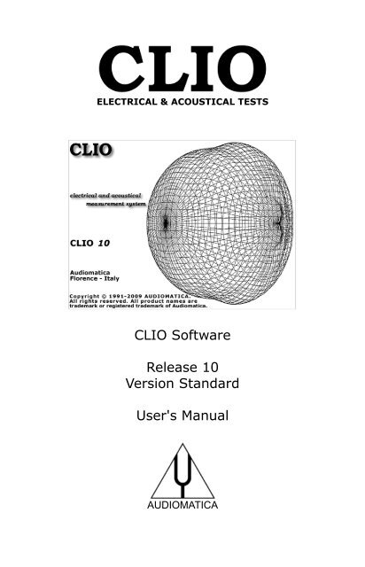
ELECTRICAL & ACOUSTICAL TESTS
CLIO Software
Release 10
Version Standard
User's Manual
AUDIOMATICA

© Copyright 1991–2010 by AUDIOMATICA SRL
All Rights Reserved
Edition 10.10, 2010/12
IBM is a registered trademark of International Business Machines Corporation.
Windows is a registered trademark of Microsoft Corporation.

CONTENTS
1 INTRODUCTION............................................................11
1.1 ABOUT THIS MANUAL.........................................................................11
1.1.1 WHAT THIS USER MANUAL DOES COVER .......................................11
1.2 GENERAL CONDITIONS AND WARRANTY...............................................11
2 THE CLIO SYSTEM.........................................................15
2.1 THE FW-01 FIREWIRE AUDIO INTERFACE..............................................16
2.1.1 TECHNICAL SPECIFICATIONS........................................................16
2.2 THE MIC-01 MICROPHONE.................................................................17
2.2.1 THE MIC-02 MICROPHONE............................................................17
2.2.2 THE MIC-03 MICROPHONE............................................................17
2.2.3 TECHNICAL SPECIFICATIONS........................................................18
2.2.4 THE MIC-01 (OR MIC-02) FREQUENCY CALIBRATION DATA................18
2.2.5 THE MIC-01, MIC-02 or MIC-03 LITE MICROPHONE..........................18
2.3 THE PRE-01 MICROPHONE PREAMPLIFIER.............................................19
2.3.1 TECHNICAL SPECIFICATION..........................................................19
2.3.2 USE OF THE PREAMPLIFIER...........................................................19
2.4 THE QCBOX MODEL 5 POWER AMPLIFIER, SWITCHING AND TESTING BOX 20
2.4.1 TECHNICAL SPECIFICATIONS........................................................21
3 CLIO INSTALLATION....................................................23
3.1 MINIMUM PC CONFIGURATION............................................................23
3.2 FW-01 DRIVERS INSTALLATION UNDER WINDOWS XP............................23
3.3 FW-01 DRIVERS INSTALLATION UNDER WINDOWS VISTA AND 7.............25
3.4 SOFTWARE INSTALLATION.................................................................28
3.5 THE 'CLIO BOX'.................................................................................29
3.6 RUNNING CLIO FOR THE FIRST TIME....................................................30
3.6.1 INITIAL TEST..............................................................................30
3.7 SYSTEM CALIBRATION........................................................................32
3.7.1 CALIBRATION VALIDATION...........................................................32
3.8 CLIO SERIAL NUMBER AND DEMO MODE...............................................34
3.9 TROUBLESHOOTING CLIO INSTALLATION..............................................34
4 CLIO BASICS................................................................35
4.1 INTRODUCTION.................................................................................35
4.2 GETTING HELP...................................................................................35
4.3 CLIO DESKTOP..................................................................................36
4.4 MAIN TOOLBAR................................................................................36
4.4.1 MEASUREMENT ANALYSIS.............................................................37
4.4.2 AUTOSCALE................................................................................37
4.4.3 HELP..........................................................................................37
4.5 HARDWARE CONTROLS TOOLBAR........................................................38
4.5.1 INPUT CONTROL..........................................................................38
4.5.2 INPUT/OUTPUT LOOPBACK............................................................38
4.5.3 GENERATOR CONTROL.................................................................38
4.5.4 MICROPHONE CONTROL...............................................................40
4.5.5 SAMPLING FREQUENCY................................................................40

4.6 QCBOX & LPT CONTROLS....................................................................40
4.6.1 CONTROLLING THE QCBOX 5 POWER AMPLIFIER, SWITCHING AND
MEASURING BOX..................................................................................41
4.7 CONTROLLING TURNTABLES................................................................42
4.7.1 TURNTABLES OPTIONS DIALOG.....................................................43
4.8 MAIN MENU AND SHORTCUTS.............................................................46
4.8.1 FILE MENU..................................................................................46
4.8.2 ANALYSIS MENU..........................................................................47
4.8.3 CONTROLS MENU........................................................................51
4.8.4 WINDOWS MENU.........................................................................52
4.8.5 HELP MENU.................................................................................52
4.9 BASIC CONNECTIONS........................................................................53
4.9.1 CONNECTING THE CLIO BOX.........................................................53
4.9.2 CONNECTING A MICROPHONE.......................................................54
4.9.3 CONNECTING THE CLIOQC AMPLIFIER & SWITCHBOX......................55
5 SYSTEM OPERATIONS AND SETTINGS...........................57
5.1 INTRODUCTION.................................................................................57
5.2 REGISTERED FILE EXTENSIONS...........................................................57
5.3 FILE MENU AND MAIN TOOLBAR BUTTONS............................................58
5.3.1 LOADING AND SAVING FILES........................................................59
5.3.2 EXPORTING DATA........................................................................61
5.3.3 EXPORTING GRAPHICS.................................................................62
5.3.4 PRINTING...................................................................................62
5.4 OPTIONS..........................................................................................63
5.4.1 GENERAL....................................................................................63
5.4.2 UNITS CONVERSION....................................................................64
5.4.3 GRAPHICS..................................................................................66
5.4.4 HARDWARE.................................................................................67
5.4.5 QC AND OPERATORS AND PASSWORDS..........................................67
5.5 DESKTOP MANAGEMENT.....................................................................68
5.6 CALIBRATION....................................................................................68
5.7 STARTUP OPTIONS AND GLOBAL SETTINGS...........................................69
5.7.1 SAVING MEASUREMENT SETTINGS................................................69
6 COMMON MEASUREMENT INTERFACE...........................71
6.1 INTRODUCTION.................................................................................71
6.2 UNDERSTANDING THE DISPLAY IN FRONT OF YOU.................................71
6.2.1 STEREO MEASUREMENTS DISPLAY.................................................72
6.2.2 COLLAPSING MARKERS................................................................73
6.2.3 DIRECT Y SCALES INPUT..............................................................73
6.3 BUTTONS AND CHECKBOXES...............................................................74
6.4 HOW TO ZOOM..................................................................................75
6.5 SHORTCUTS AND MOUSE ACTIONS......................................................75
6.6 THE MLS TIME DOMAIN DISPLAY.........................................................76
7 SIGNAL GENERATOR.....................................................77
7.1 INTRODUCTION.................................................................................77
7.2 SINUSOID.........................................................................................77
7.3 TWO SINUSOIDS...............................................................................79
7.4 MULTITONES.....................................................................................80
7.5 WHITE NOISE....................................................................................81

7.6 MLS.................................................................................................82
7.7 CHIRPS............................................................................................83
7.8 PINK NOISE......................................................................................85
7.9 ALL TONES........................................................................................87
7.10 SIGNAL FILES..................................................................................89
7.10.1 SAVING SIGNAL FILES................................................................90
8 MULTI-METER...............................................................91
8.1 INTRODUCTION.................................................................................91
8.2 MULTI-METER CONTROL PANEL............................................................91
8.2.1 TOOLBAR BUTTONS.....................................................................92
8.2.2 TOOLBAR DROP DOWN LISTS........................................................92
8.3 USING THE MULTI-METER...................................................................93
8.3.1 THE MINIMIZED STATE.................................................................93
8.3.2 CAPTURING THE GLOBAL REFERENCE LEVEL...................................93
8.4 THE SOUND LEVEL METER...................................................................95
8.4.1 CAPTURING THE MICROPHONE SENSITIVITY...................................95
8.5 THE LCR METER.................................................................................97
8.5.1 MEASURING AN INDUCTOR...........................................................97
8.6 INTERACTION BETWEEN THE MULTI-METER AND FFT..............................98
9 FFT, RTA AND “LIVE” TRANSFER FUNCTION.................99
9.1 INTRODUCTION.................................................................................99
9.2 NARROWBAND FFT ANALYZER.............................................................99
9.2.1 TOOLBAR BUTTONS, DROP DOWN LISTS AND DISPLAYS.................100
9.3 RTA - OCTAVE BANDS ANALYZER........................................................101
9.3.1 DEDICATED TOOLBAR FUNCTIONS...............................................101
9.4 FFT SETTINGS DIALOG.....................................................................102
9.5 FFT AND RTA OPERATION..................................................................103
9.6 AVERAGING.....................................................................................107
9.7 TIME DATA DISPLAY (OSCILLOSCOPE)................................................108
9.8 FFT AND MULTI-METER.....................................................................109
9.9 FFT AND Leq ANALIZER....................................................................109
9.10 “LIVE” TRANSFER FUNCTION ANALYZER............................................110
9.10.1 DEDICATED ‘LIVE’ TOOLBAR FUNCTIONS....................................110
9.10.2 USING CLIO DURING A LIVE PERFORMANCE................................111
10 MLS & LOG CHIRP.....................................................115
10.1 INTRODUCTION.............................................................................115
10.2 MLS & LOG CHIRP CONTROL PANEL..................................................115
10.2.1 TOOLBAR BUTTONS..................................................................116
10.2.2 TOOLBAR DROP DOWN LISTS....................................................116
10.2.3 MLS & LOG CHIRP SETTINGS DIALOG.........................................117
10.2.4 MLS & LOG CHIRP POST-PROCESSING TOOLS..............................118
10.3 IMPULSE RESPONSE CONTROL PANEL...............................................119
10.3.1 TOOLBAR BUTTONS..................................................................119
10.4 MEASURING FREQUENCY RESPONSE.................................................120
10.4.1 MEASUREMENT LEVEL...............................................................120
10.4.2 MLS & LOG CHIRP SIZE............................................................120
10.4.3 ACOUSTIC FREQUENCY RESPONSE.............................................122
10.4.4 PHASE & GROUP DELAY............................................................126
10.5 OTHER TIME DOMAIN INFORMATION................................................130

10.6 PROCESSING TOOLS BY EXAMPLE ...................................................131
10.7 MLS Vs. LOG CHIRP........................................................................134
10.8 RELATED MENUS............................................................................136
11 SINUSOIDAL.............................................................137
11.1 INTRODUCTION ............................................................................137
11.2 SINUSOIDAL CONTROL PANEL.........................................................137
11.2.1 TOOLBAR BUTTONS..................................................................137
11.2.2 TOOLBAR DROP DOWNS...........................................................138
11.2.3 SINUSOIDAL SETTINGS DIALOG................................................139
11.2.4 SINUSOIDAL POST PROCESSING TOOLS.....................................141
11.3 HOW TO MEASURE A SIMULTANEOUS FREQUENCY AND IMPEDANCE
RESPONSE OF A LOUDSPEAKER................................................................142
11.3.1 SETTING UP THE FREQUENCY RESPONSE....................................142
11.3.2 SETTING UP THE IMPEDANCE RESPONSE....................................143
11.3.3 INTEGRATING THE TWO-CHANNELS MEASUREMENT.....................144
11.4 A BRIEF DESCRIPTION ON SETTINGS EFFECTS...................................146
11.4.1 STEPPED VS. NOT STEPPED.......................................................146
11.4.2 FREQUENCY RESOLUTION.........................................................147
11.4.3 GATING..................................................................................148
11.5 DISTORTION AND SETTINGS............................................................150
12 WATERFALL , DIRECTIVITY & 3D..............................153
12.1 INTRODUCTION.............................................................................153
12.2 WATERFALL, DIRECTIVITY & 3D CONTROL PANEL...............................155
12.2.1 COMMON TOOLBAR BUTTONS AND DROP DOWN LISTS.................155
12.3 WATERFALL SPECIFIC CONTROLS.....................................................156
12.3.1 WATERFALL SETTINGS..............................................................156
12.3.2 WATERFALL OPERATION............................................................157
12.4 MAKING A CUMULATIVE SPECTRAL DECAY.........................................158
12.5 DIRECTIVITY SPECIFIC CONTROLS...................................................161
12.5.1 DIRECTIVITY SETTINGS AND OPERATION....................................162
12.6 MEASURING LOUDSPEAKER SINGLE POLAR DATA (1D MODE)..............164
12.6.1 PREPARING AUTOSAVE AND THE MLS CONTROL PANEL.................164
12.6.2 PREPARING THE TURNTABLE.....................................................165
12.6.3 TAKING THE MEASUREMENTS....................................................165
12.7 REPRESENTING SINGLE POLAR DATA................................................167
12.8 3D SPECIFIC CONTROLS.................................................................169
12.8.1 3D SETTINGS AND OPERATION..................................................169
12.9 MEASURING LOUDSPEAKER SINGLE POLAR DATA (3D MODE)..............172
12.9.1 PREPARING AUTOSAVE AND THE MLS CONTROL PANEL.................172
12.9.2 PREPARING THE TURNTABLES....................................................172
12.9.3 TAKING THE MEASUREMENTS....................................................173
12.10 MEASURING FULL SPHERE LOUDSPEAKER POLAR DATA (3D MODE).....174
12.10.1 PREPARING AUTOSAVE AND THE MLS CONTROL PANEL...............174
12.10.2 PREPARING THE TURNTABLES..................................................174
12.10.3 TAKING THE MEASUREMENTS..................................................175
12.11 REPRESENTING 3D BALLOON DATA.................................................176
12.12 EXPORT 3D BALLOON DATA............................................................178
12.12.1 EXPORT EASE .XHN AND CLF V2 .TAB FILES...............................179
12.12.2 EXPORT SET OF IMPULSE RESPONSES......................................180
12.13 H+V MODE...............................................................................180

13 MEASURING IMPEDANCE AND T&S PARAMETERS......181
13.1 INTRODUCTION.............................................................................181
13.2 GENERALS.....................................................................................181
13.3 INTERNAL MODE............................................................................181
13.3.1 MEASURING IMPEDANCE OF LOUDSPEAKERS..............................183
13.3.2 SETTING THE RIGHT LEVEL.......................................................183
13.3.3 DEALING WITH ENVIRONMENTAL NOISE.....................................184
13.3.4 DEALING WITH VIBRATIONS......................................................185
13.4 I SENSE........................................................................................186
13.5 CONSTANT VOLTAGE & CONSTANT CURRENT.....................................187
13.5.1 CONSTANT VOLTAGE................................................................187
13.5.2 CONSTANT CURRENT................................................................189
13.6 IMPEDANCE: SINUSOIDAL OR MLS...................................................191
13.7 THIELE & SMALL PARAMETERS.........................................................192
13.7.1 INTRODUCTION.......................................................................192
13.7.2 T&S PARAMETERS CONTROL PANEL ...........................................192
13.7.3 GLOSSARY OF SYMBOLS...........................................................193
13.7.4 T&S STEP BY STEP...................................................................194
13.7.5 USING LSE (LEAST SQUARE ERROR)...........................................196
14 LINEARITY & DISTORTION ......................................197
14.1 INTRODUCTION.............................................................................197
14.2 LINEARITY & DISTORTION CONTROL PANEL.......................................197
14.2.1 TOOLBAR DROP DOWN LIST......................................................198
14.2.2 LINEARITY & DISTORTION SETTINGS DIALOG .............................198
15 ACOUSTICAL PARAMETERS.......................................201
15.1 INTRODUCTION.............................................................................201
15.2 THE ACOUSTICAL PARAMETERS CONTROL PANEL...............................201
15.2.1 TOOLBAR BUTTONS AND DROP DOWN LISTS...............................202
15.2.2 INTERACTION WITH THE A.P. CONTROL PANEL............................203
15.3 ACOUSTICAL PARAMETERS SETTINGS...............................................204
15.4 THE CALCULATED ACOUSTICAL PARAMETERS....................................205
15.5 NOTES ABOUT ACOUSTICAL PARAMETERS MEASUREMENT...................206
15.6 STI CALCULATION..........................................................................207
16 Leq LEVEL ANALYSIS................................................211
16.1 INTRODUCTION.............................................................................211
16.2 THE Leq CONTROL PANEL................................................................211
16.2.1 TOOLBAR BUTTONS AND DROP DOWN LISTS...............................212
16.2.2 INTERACTION WITH THE Leq CONTROL PANEL.............................213
16.3 Leq SETTINGS...............................................................................214
17 WOW AND FLUTTER..................................................215
17.1 INTRODUCTION.............................................................................215
17.2 WOW & FLUTTER CONTROL PANEL....................................................215
17.2.1 TOOLBAR BUTTON....................................................................215
17.2.2 TOOLBAR DROP DOWN LIST......................................................215
17.3 FEATURES.....................................................................................216

18 WAVELET ANALYSIS.................................................219
18.1 INTRODUCTION.............................................................................219
18.2 WAVELET ANALYSIS CONTROL PANEL................................................220
18.2.1 COMMON TOOLBAR BUTTONS AND DROP DOWN LISTS.................220
18.3 WAVELET ANALYSIS SETTINGS.........................................................221
18.4 WAVELET ANALYSIS OPERATION.......................................................222
18.4.1 TRADING BANDWIDTH AND TIME RESOLUTION............................222
18.4.2 NORMALIZED SCALOGRAMS .....................................................224
BIBLIOGRAPHY.............................................................227
NORMS..........................................................................229

1 INTRODUCTION
1.1 ABOUT THIS MANUAL
This User's Manual explains the CLIO system hardware and CLIO 10 software.
All software versions are covered, please note that CLIO 10 software is designed to
operate in conjunction with the supplied PC hardware. If the hardware is absent or
the serial numbers do not correspond then CLIO 10 will operate in demo mode
only.
1.1.1 WHAT THIS USER MANUAL DOES COVER
The CLIO System is a complete electro-acoustic analyzer. There are thousands of
books on many of the topics that CLIO handles as a measurement system. The
simple definition of Frequency Response could be extended to a book itself. This
User Manual is intended only as a guide to allow the user to quickly become
efficient in using the CLIO system, its user interface, its hardware features and
limits. Every topic is handled through real life examples with dozens of actual
measurement being presented for clarity. It is therefore a HOW TO manual; WHY is
left to the reader to explore through other literature and should be considered as
essential reading. There is however reference [1], 'Testing Loudspeakers' by Joseph
D'Appolito, which, in our opinion, is the perfect complement of what is covered
here. Anyone who feels that WHY and HOW is strongly related should seriously
consider buying this wonderful book.
1.2 GENERAL CONDITIONS AND WARRANTY
THANKS
Thank you for purchasing your CLIO system. We hope that your experiences using
CLIO will be both productive and satisfying.
CUSTOMER SUPPORT
Audiomatica is committed to supporting the use of the CLIO system, and to that
end, offers direct support to end users. Our users all around the world can contact
us directly regarding technical problems, bug reports, or suggestions for future
software enhancements. You can call, fax or write to us at:
AUDIOMATICA SRL
VIA MANFREDI 12
50136 FLORENCE, ITALY
PHONE: +39-055-6599036
FAX: +39-055-6503772
AUDIOMATICA ON-LINE
For any inquiry and to know the latest news about CLIO and other Audiomatica’s
products we are on the Internet to help you:
AUDIOMATICA website: www.audiomatica.com
E-MAIL: info@audiomatica.com
1 INTRODUCTION 11

AUDIOMATICA’S WARRANTY
Audiomatica warrants the CLIO system against physical defects for a period of one
year following the original retail purchase of this product. In the first instance,
please contact your local dealer in case of service needs. You can also contact us
directly as outlined above, or refer to other qualified personnel.
WARNINGS AND LIMITATIONS OF LIABILITY
Audiomatica will not assume liability for damage or injury due to user servicing or
misuse of our product. Audiomatica will not extend warranty coverage for damage
of the CLIO system caused by misuse or physical damage. Audiomatica will not
assume liability for the recovery of lost programs or data. The user must assume
responsibility for the quality, performance and the fitness of Audiomatica software
and hardware for use in professional production activities.
The CLIO SYSTEM, CLIOfw, CLIOQC and AUDIOMATICA are registered trademarks
of Audiomatica SRL.
12 1 INTRODUCTION

REGISTRATION CARD
AUDIOMATICA REGISTRATION CARD
(EMAIL OR FAX TO US)
CLIO SERIAL NUMBER: ______________________________
SOFTWARE VERSION: _______________________________
PURCHASE DATE: ___________________________________
NAME: ___________________________________________
JOB TITLE: ________________________________________
COMPANY: ________________________________________
ADDRESS: ________________________________________
ZIP OR POST CODE: ________________________________
PHONE NUMBER: ___________________________________
FAX NUMBER: _____________________________________
E-MAIL: __________________________________________
1 INTRODUCTION 13

2 THE CLIO SYSTEM
Depending on the hardware options that have been purchased, the CLIO system
consists of the following components:
– The FW-01 firewire audio interface
– The MIC-01 or MIC-02 or MIC-03 (also Lite) microphones
– The PRE-01 microphone preamplifier
– The QCBox Model 5 power amplifier, switching and testing box
In the next few pages we will describe each component and give its respective
technical specifications.
NOTE: Audiomatica reserves the right to modify the following specifications without
notice.
2 THE CLIO SYSTEM 15

2.1 THE FW-01 FIREWIRE AUDIO INTERFACE
The FW-01 Firewire Audio Interface sets new hardware precision standards for the
CLIO System. The FW-01 unit has been designed to be a complete two channels
professional A/D D/A audio front-end for your PC; it is connected to the computer
by an IEEE-1394 link giving you maximum performances; it can be powered by the
same link giving you maximum portability. The FW-01 performances (24 bit @ 192
kHz) represent state-of-the-art measurement capabilities for any audio device or
acoustical test. The FW-01 is equipped with an instrument grade balanced input and
output analog circuitry with an exceptionally wide range of output attenuation and
input gain that allows an easy interface to the outer world; the input and output
loopback capability with the internal ultra stable voltage reference permit a simple
and precise calibration of the whole instrument. A switchable phantom power
supply lets you directly connect an Audiomatica MIC-01, MIC-02 or MIC-03 as well
as any other standard balanced microphone to any of the FW-01 input.
2.1.1 TECHNICAL SPECIFICATIONS
GENERATOR
Two channels 24 Bit sigma-delta D/A Converter
Frequency range: 1Hz-90kHz
Frequency accuracy: >0.01%
Frequency resolution: 0.01Hz
Output impedance: 660Ohm
Max output level (Sine):17dBu (5.5Vrms)
Attenuation: 0.1 dB steps to full mute
THD+Noise(Sine):0.008%
Digital out: SPDIF
ANALYZER
Two channels 24 bit sigma-delta A/D Converter
Input range: +40 ÷ -40dBV
Max input acceptance: +40dBV (283Vpp)
Input impedance: 128kOhm (5.6kOhm mic)
Phantom power supply: 24V
PC SYSTEM RESOURCES
One free IEEE1394 port
MISCELLANEOUS
Sampling frequencies: 192kHz, 96kHz and 48kHz.
Connections: analog 2 XLR combo in, 2 XLR plus 2 RCA out, 1 RCA digital out
Digital connection: 6-pin IEEE1394
Power supply: IEEE1394 or 12V DC
Dimensions :16(w)x17(d)x4(h)
Weight: 0.8 kg
16 2 THE CLIO SYSTEM

2.2 THE MIC-01 MICROPHONE
The MIC-01 microphone is an electret measuring microphone that is particularly
well suited to being used in conjunction with the other components of the CLIO
system. It is furnished with its own stand adapter and a calibration chart reporting
the individually measured sensitivity, all fitted in an elegant case. Its long and thin
shape renders it ideal for anechoic measurements. Because its frequency response
is very flat over the entire audio band, no particular correction is usually needed.
2.2.1 THE MIC-02 MICROPHONE
The MIC-02 microphone is functionally identical to MIC-01. It differs only in the fact
that its length is 12 cm instead 25 cm. The MIC-02 is more practical to handle and
to work with, and is ideal for measurements in a reverberant environment.
2.2.2 THE MIC-03 MICROPHONE
The MIC-03 microphone is functionally identical to MIC-01. It differs only in the fact
that its length is 7 cm instead 25 cm. The MIC-03 is more convenient where space
saving is a must.
2 THE CLIO SYSTEM 17

2.2.3 TECHNICAL SPECIFICATIONS
MIC-01
Type:
Accuracy:
Maximum level:
Dimensions:
Accessories:
MIC-02:
MIC-03:
Polar Response:
Condenser electret
±1 dB, 20 Hz to 10 kHz
±2 dB, 10 kHz to 20 kHz (direct field)
130 dB SPL
8 mm diameter, 25 cm long
wooden case, 2.7 m cable, stand adapter
Same as MIC-01, but 12 cm long.
Same as MIC-01, but 7 cm long.
MIC-01-MIC-02-MIC-03
2.2.4 THE MIC-01 (OR MIC-02) FREQUENCY CALIBRATION DATA
The microphones MIC-01 and MIC-02 can be furnished with (or be submitted for) a
frequency calibration certificate. This document, along with numerical data on
floppy disk, is released by Audiomatica and specifies the frequency behavior of the
single microphone under test. The file data can be used with the CLIO software (see
5.4.2).
2.2.5 THE MIC-01, MIC-02 or MIC-03 LITE MICROPHONE
In the Lite version of MIC-01, MIC-02 and MIC-03 the accessories (wooden case,
2.7 m cable and stand adapter) are not supplied. The microphone comes as in
figure.
18 2 THE CLIO SYSTEM

2.3 THE PRE-01 MICROPHONE PREAMPLIFIER
The microphone preamplifier PRE-01 has been designed to match Audiomatica’s
microphones MIC-01, MIC-02 and MIC-03. It is particularly useful when the
microphone has to be operated far from the analyzer or when weighted
measurements are needed. PRE-01 powers the microphone connected to its input
with an 8.2V phantom supply and adds a selectable weighting filter (A or B or C);
also available there is a 20 dB gain stage. The unit is operated with one standard
9V battery or with an external DC power supply.
2.3.1 TECHNICAL SPECIFICATION
Frequency response:
7Hz÷110kHz (-3dB)
Weighting filter: A, B, C (IEC 651 - TYPE I)
Phantom power supply:
8.2V (5600 Ohm)
Gain:
0 & 20dB (INTERNAL SETTINGS)
Input impedance:
5600 Ohm
Output impedance:
100 Ohm
Maximum output voltage (@1kHz): 25 Vpp
THD (@1kHz): 0.01%
Input noise (@20dB gain):
7uV LIN, 5.3uV A
Drive capability:
±7mA
Batteries duration:
>24h (alkaline cell)
Size:
12.5(w)x19(d)x5(h)cm
Weight:
900g
2.3.2 USE OF THE PREAMPLIFIER
The MIC-01 or MIC-02 or MIC-03 microphone cable should be connected to the
preamplifier input while the preamplifier output requires connection to the analyzer
input. The unit is switched on with the POWER switch, while the TEST push-button
controls the state of the unit. Correct operation of the unit is indicated by the led
light being illuminated, if the LED fails to illuminate then either the batteries are low
or the external power supply is not connected. The FILTER switch inserts the
weighting filter. To choose the desired weighting filter type and to set the amplifier
gain you have to modify the unit settings with the dip switch operated from the
back panel.
NOTE: if the 20 dB gain stage is inserted the overall sensitivity (microphone + pre)
is 10 times higher. For example if your microphone has a sensitivity of 17.1 mV/Pa
and you amplify it by 20 dB then you get a sensitivity of 171 mV/Pa.
2 THE CLIO SYSTEM 19

2.4 THE QCBOX MODEL 5 POWER AMPLIFIER, SWITCHING AND
TESTING BOX
The QCBOX Model 5 power amplifier, switching and testing box is of invaluable help
when configuring an automatic or manual quality control setup, or even in everyday
laboratory use.
It can be configured, under software control via USB, to assist frequency
response and impedance measurements or to perform DC measurements.
Between its features is the possibility of internal switching that permits the
measurement of the impedance and frequency response of the loudspeaker
connected to its output sockets without changing the wiring to the speaker; it
is also possible to route one of four inputs for the response measurements; these
input have powering for a microphone (0÷24V variable).
An internal ADC measures the DC current into the voice coil; an over current limiter
is available to a predefined threshold. Thanks to an internal software controlled
voltage generator the speaker can be driven with a superimposed DC voltage
(±20V max), allowing for measurements of large signal T&S parameters. Two ADC
converters with a ±2.5V and ±5V are available at inputs 3 and 4 to measure the
displacement with a laser sensor or any other DC signal.
A dedicated output, ISENSE, allows impedance measurements in constant voltage
mode as well as voice coil current distortion analysis.
A 5 bit in - 6 bit out digital port is available to interface the QCBOX with external
hardware or line automation. An ulterior dedicated input permits an external foot
pedal switch to be connected and trigger QC operations.
20 2 THE CLIO SYSTEM

19” RACK MOUNT ASSEMBLY
Using the Rack QC panel it is possible to assemble the QCBOX Model 5 together the
FW-01 Audio Interface so that they can be mounted in a standard 19” rack frame.
2.4.1 TECHNICAL SPECIFICATIONS
Inputs:
Four line/microphone inputs with
selectable phantom power supply (0÷24V variable)
One TTL input for external trigger
5 digital lines
Outputs:
Isense
6 digital lines
Functions:
USB controlled internal switches for impedance
and DC measurements
DC measuring: Isense current ±2.25 A
DC IN 3 ±2.5 V
DC IN 4 ±5 V
Power output stage: 50W (8Ohm) with current sensing and overcurrent protection
Possibility of superimposing a DC voltage (±20 V)
THD (@1 kHz): 0.004 %
Dimensions: 23(w)x23(d)x4(h)cm
Weight:
1.4kg
AC: 90÷240V
2 THE CLIO SYSTEM 21

3 CLIO INSTALLATION
3.1 MINIMUM PC CONFIGURATION
The CLIO FW-01 firewire audio interface running the CLIO software can be installed
in any personal computer with the following minimum system requirements:
– Pentium IV processor (suggested minimum 1GHz)
– One free IEEE-1394 port
– 256 MB RAM
– 1024x786 video adapter
– Microsoft Windows XP or Vista
– Adobe Acrobat Reader
DO NOT CONNECT THE FW-01 UNIT TO THE PC UNTIL REQUESTED!
If you are installing under:
- Windows XP go to section 3.2
- Windows Vista and 7 go to section 3.3
3.2 FW-01 DRIVERS INSTALLATION UNDER WINDOWS XP
The procedures described refer specifically (and are described with examples and
figures) to the Windows XP Professional operating system, English version, they
can be applied with only minor modifications and appropriate translations to all
languages and to Windows XP Home.
To install the FW-01 drivers in your computer you should follow the instructions
presented below:
1) Insert the CLIO 10 CD ROM in the computer.
2) Wait for autorun application or run "Clioinstall.exe".
3) Choose "FW-01 DRIVERS" to start installation.
3 CLIO INSTALLATION 23

WHEN PROMPTED CONNECT THE FW-01 UNIT!
To connect the FW-01 unit to your PC you need to do the following:
1) Locate an IEEE-1394 port on your PC. You may either use a standard 6-pin port
(with or without power supply) or a standard 4-pin (small connector, without
power supply) port.
2) If you use a 6-pin port use the supplied 6-pin-to-6-pin cable. If you use a 4-pin
port please provide an IEEE 1394 6-pin-to-4-pin cable (often referred as i-Link).
3) If you use a 6-pin port verify that it is capable of power supply.
4) If you use a 6-pin port without power supply or a 4-pin port you must also
provide a 12V external power supply.
Ignore Microsoft's warning message about Digital Signature, answer 'Yes' to the
prompt and reach the end of the wizard.
You will then reach the end of the wizard.
24 3 CLIO INSTALLATION

Let's now verify the correct installation of the FW-01 driver. Click with the right
mouse button on the 'My Computer' icon on the Windows desktop. Then click
'Properties', select the 'Hardware' tab and press the 'Device Manager' button as in
the following figure.
Verify the presence of the 'Clio Firewire' driver under the 61883 device class.
Your driver installation was successful!
3.3 FW-01 DRIVERS INSTALLATION UNDER WINDOWS VISTA AND 7
The procedures described refer specifically (and are described with examples and
figures) to the Windows 7 operating system, English version, they can be applied
with only minor modifications and appropriate translations to all languages.
To install the FW-01 drivers in your computer you should follow the instructions
presented below:
1) Insert the CLIO 10 CD ROM in the computer.
2) Wait for autorun application or run "Clioinstall.exe".
3) Choose "FW-01 DRIVERS" to start installation.
WHEN PROMPTED CONNECT THE FW-01 UNIT!
3 CLIO INSTALLATION 25

To connect the FW-01 unit to your PC you need to do the following:
1) Locate an IEEE-1394 port on your PC. You may either use a standard 6-pin port
(with or without power supply) or a standard 4-pin (small connector, without
power supply) port.
2) If you use a 6-pin port use the supplied 6-pin-to-6-pin cable. If you use a 4-pin
port please provide an IEEE 1394 6-pin-to-4-pin cable (often referred as i-Link).
3) If you use a 6-pin port verify that it is capable of power supply.
4) If you use a 6-pin port without power supply or a 4-pin port you must also
provide a 12V external power supply.
You will then reach the end of the wizard.
Let's now verify the correct installation of the FW-01 driver. Click with the right
mouse button on the 'My Computer' icon on the Windows desktop or on the Start
Menu. Then click 'Properties', press the 'Device Manager' link as in the following
figure.
26 3 CLIO INSTALLATION

Verify the presence of the 'Clio Firewire' driver under the 61883 device class.
Your driver installation was successful!
3 CLIO INSTALLATION 27

3.4 SOFTWARE INSTALLATION
This paragraph deals with software installation.
The CLIO software is provided either on its own CD-ROM or, in electronic format, as
a single, self-extracting, executable file.
Be sure to have administrative rights when installing CLIO.
To install the CLIO 10 software in your computer you should follow the instructions
presented below:
1) Insert the CLIO 10 CD ROM in the computer.
2) Wait for autorun application or run "Clioinstall.exe".
3) Choose "CLIO 10 SOFTWARE" to start installation.
The procedure is completely automatic and will only request you to accept the
Software End User's License Agreement and input some information in order to
correctly install CLIO 10; the software installer will also check your operating
system version.
After successfully completing this procedure take note of the installation directory
of CLIO (usually C:\Program Files\Audiomatica\CLIO 10).
28 3 CLIO INSTALLATION

3.5 THE 'CLIO BOX'
A few words about the FW-01 firewire audio interface.
Figure 3.26
This unit is needed to correctly interface analog signals to your PC; it is also
important as it has an internal reference used to calibrate the system and also
stores the system's serial number inside its internal EEPROM; Fig.3.27 shows where
is located your CLIO system serial number.
Figure 3.27
The serial number is very important and should be mentioned each time you get in
contact with Audiomatica, either for technical support or for software upgrade.
When using your CLIO system you will normally use the FW-01 front connectors. As
you'll become extremely familiar with this hardware unit we are going to give it a
nickname: from now on we will call it 'the CLIO Box'. Also the CLIO software
refers to it with this nickname.
3 CLIO INSTALLATION 29

3.6 RUNNING CLIO FOR THE FIRST TIME
If you have completed the preceding installation procedure, you are ready to run
CLIO!
The following steps will guide you through a complete verification of the
system performance and operation.
From the Start Menu choose Programs, then CLIO 10 and click on the CLIO icon.
The program should start smoothly and present the main desktop.
If the the system is not calibrated, as the first time you run it, you will receive the
following message.
Should CLIO display an error message take note of it and go to the troubleshooting
section (3.9).
3.6.1 INITIAL TEST
Let's now execute our first test measurement - play and capture a 1kHz
sinusoid.First of all click on the In-Out Loop button for channel A; in this way the
CLIO Box connects output A with input A with an internal relay. This connection is
very important as it lets you capture and analyze a signal generated by CLIO
without the need for an external connecting cable.
Then click on the generator icon to play the 1kHz sinusoid (1031.25Hz to be
exact; more on this later, it's the default signal). Then press the F4 keystroke to
invoke the Multi-Meter as in Fig.3.28.
30 3 CLIO INSTALLATION

Figure 3.28
If everything is OK you should obtain a reading of circa 1V, variable between a
minimum of 0.95V and a maximum of 1.05V, which is the mean output level of a
sinusoidal signal when the system is not calibrated.
Now press the FFT button (or CTRL-F), then press the Oscilloscope button and
finally the GoButton.
The result you should obtain is an FFT analysis of the 1kHz sinusoid (one spectral
line @ 1kHz at 0dBV) and its time representation given by its oscillogram.
IMPORTANT NOTE: Only if these two initial tests gave correct results, as
described, go to the following paragraph and execute the system calibration; if you
are not able to obtain these results and they seem in any way corrupted do not
execute calibration and contact technical support.
3 CLIO INSTALLATION 31

3.7 SYSTEM CALIBRATION
This section describes how to perform the system calibration.
Be sure that, any time you perform a calibration, the system has warmed up for, at
least 15-20 minutes.
Select Calibration from the File menu (5.6);
Leave the CLIO Box front plugs unconnected.
Answer OK to the initial prompt; this will run an automatic procedure that will last
several minutes. The calibration procedure is completely automatic and several
progress indicators will accompany all the executed measurements. At the end of it
your CLIO system should be calibrated and ready to carry out measurements.
At the end of the calibration process it is always mandatory to verify the calibration
itself; this is done by two simple measurements as described in the following
section.
3.7.1 CALIBRATION VALIDATION
Figure 3.29
32 3 CLIO INSTALLATION

To verify the calibration first check that the generator output level is set to 0dBV
(refer to 4.5.3 for details).
Press the channel A In-Out Loop button .
Then click on the MLS button to invoke the MLS control panel. Press the Go
button to execute an MLS frequency response measurement; after about 1 second
you should obtain the desired result, a straight line (black) as in Fig.3.29. You can
click on the graph and inspect the amplitude of the measured signal: you should
obtain a reading around -3dBV, this is the correct output level of the MLS signal
with the generator output set to 0dBV.
Now click on the Sinusoidal button to invoke the Sinusoidal control panel as in
Fig.3.29. Press the Go button to execute a Sinusoidal frequency response
measurement; after about 5 seconds you should obtain the desired result, again a
straight line (black) as in Fig.3.29. You can click on the graph and inspect the
amplitude of the measured signal: you should obtain a reading around 0dBV.
To ensure a 100% correct calibration you also need to inspect the phase responses
of both measurements. To do this press the phase button and verify that you
obtain a straight line (red curves in Fig.3.29) the readings in this case should be
around zero degrees in both cases.
As a final test repeat the 1kHz tone test described in 3.6.1. The expected result is
shown in Fig.3.30.
Figure 3.30
3 CLIO INSTALLATION 33

3.8 CLIO SERIAL NUMBER AND DEMO MODE
Each CLIO system has its own serial number which plays an important role since
the CLIO software is hardware protected and relies on a correct serialization in
order to run.
Refer to 3.5 to identify your system's serial number.
If the CLIO software doesn't find a CLIO Box with a correct serial number it gives a
warning message and enters what is called DEMO mode; in this way it is possible
to run CLIO in a PC where the CLIO hardware is not installed while still allowing you
to perform post-processing and other off line jobs.
3.9 TROUBLESHOOTING CLIO INSTALLATION
To receive assistance please contact Audiomatica at info@audiomatica.com or
connect to our website www.audiomatica.com.
34 3 CLIO INSTALLATION

4 CLIO BASICS
4.1 INTRODUCTION
This chapter gives you the basic information about CLIO and the related hardware
and how to connect and operate it, while the following chapters explain in more
detail the individual measurements available to users of CLIO. Chapter 5 deals with
other general functionality of CLIO.
Here you will find information about:
- Help
- Main desktop, toolbars and menu
- Shortcuts
- Generator, Input and Output, Microphone
- Amplifier & SwitchBox, Turntable
- Connections
4.2 GETTING HELP
Figure 4.1 CLIO Help On-Line
To request the CLIO on-line help press F1. The on-line help screen (Fig. 4.1) should
appear and the context-sensitive search should locate the page appropriate to the
currently active menu, dialog or control.
Note: in order for the CLIO help to work you should have Adobe Acrobat Reader
installed on your system. The CLIO CD-ROM contains a correct version of this
utility. Refer to Adobe (www.adobe.com) for any further information.
The CLIO help can be invoked also from outside CLIO; to do this go to the Start
Menu, then Programs, then CLIO and then click on 'CLIO Help'; in this way Acrobat
will let you read and print this User Manual.
If you are not familiar with Acrobat, please spend some time to familiarize yourself
with its capabilities, controls and navigation buttons.
Another way to obtain help is through the Help Menu (see 4.6.5) which gives you
the possibility to view the on-line resources available in the Audiomatica and CLIO
websites.
4 CLIO BASICS 35

4.3 CLIO DESKTOP
The CLIO desktop presents itself as in Fig. 4.2 and gives you access to the main
menu, the (upper) main toolbar and the (lower) hardware controls toolbar.
Figure 4.2 CLIO Desktop
Inside the main toolbar and the hardware controls toolbar you can locate several
distinct functional areas as shown in the above figure. There now follows a
description of all the controls inside the two toolbars. Refer to Section 4.8 for a
detailed view inside the main menu.
4.4 MAIN TOOLBAR
Please refer to Chapter 5 for information about File and Print functions, Options
and Desktop control.
36 4 CLIO BASICS

4.4.1 MEASUREMENT ANALYSIS
By clicking on these toolbar buttons it is possible to interact and display each
measurement control panel. Once the toolbar button is clicked the appropriate
panel will be opened or reactivated. Any currently active panel will automatically be
deactivated on activation of the new one.
The same functionality will be obtained with the relative shortcuts or by making a
selection inside the Analysis Menu (see 4.6.2); a third way is to select a window
through the Windows Menu (see 4.8.4).
Enters the MLS&LogChirp Analysis control panel.
Enters the Waterfall,Directivity&3D control panel.
Enters the Wavelet Analysis control panel.
Enters the Acoustical Parameters control panel.
Enters the FFT&RTA Analysis control panel.
Enters the Sinusoidal Analysis control panel.
Enters the Multimeter control panel.
Enters the Thiele&Small Parameters control panel.
Enters the Wow&Flutter control panel.
Enters the Leq control panel.
Enters the Linearity&Distortion control panel.
Enters the Loudness Rating calculator.
Enters the Quality Control Processor.
4.4.2 AUTOSCALE
Enables autoscale. When autoscale is active the software, during measurements,
determines the optimum Y-scale settings.
4.4.3 HELP
Invokes the Help control panel.
Invokes the Internet On-Line Help.
4 CLIO BASICS 37

4.5 HARDWARE CONTROLS TOOLBAR
4.5.1 INPUT CONTROL
channel A input peak meter
Constantly monitors channel A input signal level vs.full digital input scale.
Controls channel A input polarity.
channel A input sensitivity display & control buttons
Displays the actual input sensitivity (in dBV) of the instrument, i.e. the voltage
level beyond which the hardware saturates. It is possible to modify it in 10dB
steps by pressing the (F9) and/or (F10) buttons.
channel B input peak meter
Constantly monitors channel B input signal level vs.full digital input scale.
Controls channel B input polarity.
channel B input sensitivity display & control buttons
Displays the actual input sensitivity (in dBV) of the instrument, i.e. the voltage
level beyond which the hardware saturates. It is possible to modify it in 10dB
steps by pressing the (SHIFT+F9) and/or (SHIFT+F10) buttons.
Links input channels full scale level controls. If this button is pressed the two
channel sensitivities are set equal and channel A controls act also on channel B.
Selects the Autorange mode. When in autorange mode the input sensitivity is
automatically adjusted by the instrument to achieve the optimum signal to noise
ratio.
4.5.2 INPUT/OUTPUT LOOPBACK
The CLIO Box features an internal loopback which is very useful for performing self
tests.
Connects channel A output to channel A input with an internal relay.
Connects channel B output to channel B input with an internal relay.
4.5.3 GENERATOR CONTROL
CLIO's generator can be controlled from the dedicated toolbar buttons and dialogs;
for a reference about the possible kind of signal you may generate please see
chapter 7.
output level display & control buttons
Displays the actual output level (usually in dBu) of the internal generator. This
level is valid for both output channels. It is possible to modify it in 1dB steps
pressing the (F7) and or (F8) buttons. If the Shift key is pressed
simultaneously then the steps are of 0.1dB increments.
38 4 CLIO BASICS

It is also possible to input a numeric value directly with the following dialog
which pops up when you click on the output level display.
In this case (manual input) the output level will be approximated with a 0.01dB
precision.
If you right-click on the output level display you invoke the out units pop up
from which it is possible to select the output level unit among dBu, dBV, V and
mV.
Checking the Unbalanced option the output level display is referred to the
unbalanced outputs of the Clio Box. When this mode is selected the generator
output level display is shown in white with black background.
Switches on and off the generator.
Use the ESC key to immediately kill the generator .
If you wish to receive a confirmation message (Fig.4.3) before playing the
generator then check the appropriate box in the General Options dialog (5.4).
Figure 4.3
generator drop down menu
Clicking on the small arrow beside the generator button will invoke the generator
drop down menu, from there it is possible to choose the output signal type to be
generated. The default signal at startup is a 1031.25Hz sinusoid.
Refer to Chapter 7 Signal Generator for a detailed description of all generated
signals.
4 CLIO BASICS 39

4.5.4 MICROPHONE CONTROL
Switches Channel A 24V phantom power on and off. This supply is capable of
operating any balanced microphone and also to operate Audiomatica's
microphones MIC-01, MIC-02 and MIC-03 (see later).
Switches Channel B 24V phantom power on and off.
To enter the microphone sensitivity please refer to 5.4 Options.
4.5.5 SAMPLING FREQUENCY
Indicates the current sampling frequency of the instrument. To change
it simply click on it and refer to 5.4 Options.
4.6 QCBOX & LPT CONTROLS
Enters the External Hardware Controls dialog box. This dialog box performs
controls over some external hardware connected to the computer.
Fig. 4.6 External Hardware Controls dialog box
This control panel helps you when you are operating the CLIOQC Amplifier &
SwitchBox.
You may choose the Amplifier & SwitchBox model and set the value of the internal
sensing resistor to obtain maximum precision during impedance measurements (for
this please refer to chapter 13).
These controls are self-explanatory; they are also covered in the unit's user's
manual, in this manual, and everywhere else the amplifier and switchbox is used.
40 4 CLIO BASICS

You can also read and write a PC parallel port:
4.6.1 CONTROLLING THE QCBOX 5 POWER AMPLIFIER, SWITCHING
AND MEASURING BOX
With this dialog box it is possible to access to the QCBox 5 enhanced features. It is
possible to superimpose a DC voltage on the amplifier output, set the microphones
phantom voltage and the output current protection threshold. It is also possible to
read the Isense DC current and the IN 3 and IN 4 DC voltages.
The digital I/O port is showed on the bottom of the dialog box and monitor the port
status, it is possible to write the out bits by simply clicking on them.
Fig.4.7 QCBOX 5 power amplifier, switching and measuring box control panel
4 CLIO BASICS 41

4.7 CONTROLLING TURNTABLES
This control panel allows the control of one or two turntables. The control of two
turntables is available only with the QC software.
Using two turntables it is possible to measure the loudspeaker response in three
dimensions, i.e. the software can send commands to the turntables to aim the
loudspeaker under test in a given direction.
Fig.4.8 Turntables control panel
Reset turntable position to angle 0 by clockwise rotation (degrees up)
Reset turntable position to angle 0 by counterclockwise rotation (degrees down)
Set turntable reference angle (0 degrees)
Goto angle by clockwise rotation (degrees up)
Goto angle by counterclockwise rotation (degrees down)
Step angle by clockwise rotation (degrees up), note that the step size is a
turntable setting that cannot be accessed from CLIO
Step angle by counterclockwise rotation (degrees down)
Stop the turntable rotation
and
connect turntables and link the
turntable positions to the measurements
42 4 CLIO BASICS

Displays turntable current angle (top) and next angle (bottom), while the turntable
is rotating the bottom background is highlighted in red.
Open the Autosave Settings dialog
Reset turntable angles according to Autosave Settings
Open the Turntables Option dialog
Start an MLS Autosave measurement set
Halt an MLS Autosave measurement set
Resume an MLS Autosave measurement set
4.7.1 TURNTABLES OPTIONS DIALOG
With this dialog it is possible to choose which model of turntable to use for each
rotating axis (polar and azimuth). The software can take full control of the Outline
ET250-3D and the LinearX LT360 turntables. It support also (limited to the polar
rotation) a TTL pulse control using the PC parallel port which can be used to trigger
the Outline ET/ST turntable or any other device. Using the combo box it is
possible to choose which turntable model to use for the polar and azimuth angles
(for a definition of polar and azimuth angles please refer to chapter 12).
Outline ET250-3D
The Outline ET250-3D uses an Ethernet connection, please refer to the
manufacturer documentation to setup the device. In the option dialog it is
necessary to input the turntable IP and TCP/IP port.
Note: In order to work properly the basert.dll file must be present into the CLIO
installation directory.
4 CLIO BASICS 43

LinearX LT360
The LinearX LT360 turntable uses an USB or COM connection, please refer to the
manufacturer documentation to the setup of the device. In the option dialog it is
needed to input the communication port to be used.
Some turntables settings, such as the rotation speed and the velocity profile must
be managed using the software supplied with the turntable. For correct
operations with CLIO software the “Display Readout Polarity” setting of
the LT360 turntable must be set on “Unipolar”.
Note: In order to work properly the lt360lib.dll file must be present into the CLIO
installation directory.
The delay parameter (in milliseconds) put the software in a wait state after the
completion of the turntable rotation, this can be useful in a non anechoic space to
let the energy in the room to decay between measurements.
TTL pulse control
Selecting TTL pulse it is possible to control a turntable using a TTL signal from the
PC parallel port. This is valid only for the polar angle and with this selection
it is not possible to use two computer controlled turntables. In this case the
second turntable can be only selected as “Manual”.
The TTL pulse control uses the parallel port or the output port of a QCBox model V.
The information given here apply to the control of the Outline ET/ST Turntable;
they can be adapted to any other device.
44 4 CLIO BASICS

The control is achieved with Bit 7 of the parallel port output bits, as shown in
Fig.4.6. The turntable should be connected to the parallel port of the computer by
means of a cable defined as follows:
PC side DB25 male
ET/ST side DB9 male
Pin 9 Pin 2
Pin 22 Pin 4
All other pins unconnected
With the QCBox5 selected the control is achieved with Bit 5 of the QC Box output
port, the turntable should be connected to the QC Box V output port by means of a
cable defined as follows:
QCBox5 side DB25 male
ET/ST side DB9 male
Pin 6 Pin 2
Pin 14 Pin 4
All other pins unconnected
The cable should be connected as in the following figure.
Fig.4.9 Outline ET/ST Turntable connections
Inside the Turntable Option panel it is possible to set its Resolution (in degrees)
and Speed (in rotations per minute); the combination of these settings give the
software an indication about how much time to wait after the controlling pulse is
output.
Manual
For the azimuth angle only is it possible to choose the “Manual” turntable. This
means that the azimuth rotation of the loudspeaker under test must be managed
manually. Instead of automatically control the turntable, the software display a
pop-up message to the operator and wait for the completion of the manual rotation.
Please refer to chapter 12 for further information on polar measurement sets.
4 CLIO BASICS 45

4.8 MAIN MENU AND SHORTCUTS
The user should carefully read this section which gives you a comprehensive list of
all the menu and shortcuts available within CLIO. Shortcuts, i.e. keystrokes that
you can press to obtain a certain action, will save you time and increase your
productivity.
Also refer to Chapter 6 to learn the measurement interface and its associated
shortcuts. Note that the measurement specific (MLS submenu, FFT submenu etc.)
menus are active only when the measurement control panel is open and selected.
4.8.1 FILE MENU
Please refer to Chapter 5 for a detailed explanation of the File Menu.
Fig.4.10 File Menu
F3 Saves a measurement file relative to the active control panel.
F2 Loads a measurement file relative to the active control panel.
ALT+F2
Enters the Autosave Settings dialog box (see 5.3.1).
SHIFT+F2
Exports the active measurement as an ASCII file.
CTRL+F2
Exports the active measurement as a Windows Enhanced Metafile, BMP, PNG,
JPEG or GIF.
ALT+P
Prints the active measurement.
F6 Enables/disables the AutoScale function (see 4.4.2).
46 4 CLIO BASICS

4.8.2 ANALYSIS MENU
The Analysis menu gives you a powerful way to access the measurement menu and
menu functions, through the keyboard. Here we present you with all the available
menus and shortcuts; the shortcuts, when present, are visible from each submenu
and are listed on the right of the function; refer to the specific chapters for each
measurement for details about it.
Fig.4.11 Analysis Menu
CTRL+M
Enters the MLS&LogChirp Analysis control panel.
CTRL+W
Enters the Waterfall&Directivity control panel.
SHIFT+CTRL+W
Enters the Wavelet Analysis control panel.
CTRL+A
Enters the Acoustical Parameters control panel.
CTRL+F
Enters the FFT&RTA Analysis control panel.
CTRL+S
Enters the Sinusoidal Analysis control panel.
F4
Enters the Multimeter control panel.
CTRL+T
Enters the Thiele&Small Parameters control panel.
CTRL+Alt+W
Enters the Wow&Flutter control panel.
CTRL+L
Enters the Leq control panel.
CTRL+D
Enters the Linearity&Distortion control panel.
CTRL+Q
Enters the Quality Control Processor.
4 CLIO BASICS 47

Fig.4.12 MLS&LogChirp Submenu - Frequency and Time
Fig.4.13 Waterfall and Directivity Submenu
Fig.4.14 Wavelet Analysis SubMenu
Fig.4.15 Acoustical Parameters SubMenu
48 4 CLIO BASICS

Fig.4.16 FFT and FFT Live SubMenu
Fig. 4.17 Sinusoidal Submenu
Fig. 4.18 Multi-meter Submenu
Fig. 4.19 T&S Parameters Submenu
4 CLIO BASICS 49

Fig. 4.20 Wow&Flutter Submenu
Fig. 4.21 Leq Submenu
Fig. 4.22 Linearity&Distortion Submenu
50 4 CLIO BASICS

4.8.3 CONTROLS MENU
The Controls Menu is the heart of your CLIO hardware; learn how to access
hardware control through the keyboard in detail. Refer also to 4.4.2, 4.4.3, 4.4.4
and 4.5.
ESC
Fig. 4.23 Controls Menu
Immediately kills the generator. Equivalent to releasing
F7 Decreases the output level of 1dB. Equivalent to
SHIFT+F7
Decreases the output level of 0.1dB. Equivalent to SHIFT+
F8 Increases the output level of 1dB. Equivalent to
SHIFT+F8
Increases the output level of 0.1dB. Equivalent to SHIFT+
F10
Increases channel A input acceptance of 10dB. If the Link Button is pressed
then increases also channel B input acceptance of 10dB. Equivalent to
SHIFT+F10
Increases channel B input acceptance of 10dB. Equivalent to
F9 Decreases channel A input acceptance of 10dB. If the Link Button is pressed
then decreases also channel B input acceptance of 10dB. Equivalent to
SHIFT+F9
Decreases channel B input acceptance of 10dB. Equivalent to
4 CLIO BASICS 51

CTRL+P
Swithces channel A microphone power supply on and off. Equivalent to
CTRL+ALT+P
Swithces channel B microphone power supply on and off. Equivalent to
SHIFT+F4
Enters the QCBox and LPT control panel. Equivalent to
CTRL+F4
Enters the Turntables Controls panel. Equivalent to
F6 Enables autoscale. Equivalent to
4.8.4 WINDOWS MENU
The Windows Menu helps you manage all opened windows (i.e. measurement
control panels) in a standardized way. You can Tile or Cascade the open windows or
access each one directly.
4.8.5 HELP MENU
Fig. 4.24 Windows Menu
From the Help Menu you can access all the available help resources installed in your
computer or available directly from Audiomatica over the internet.
Fig. 4.25 Help Menu
F1 Invokes the On-Line Help.
52 4 CLIO BASICS

4.9 BASIC CONNECTIONS
In order to correctly interface CLIO with the outside world you should always keep
in mind the following electrical specifications:
MAXIMUM INPUT VOLTAGE:
MAXIMUM OUTPUT VOLTAGE:
INPUT IMPEDANCE:
OUTPUT IMPEDANCE:
+40 dBV (283 V peak-to-peak)
+18dBu (6.156Vrms) (sine)
128 kOhm
660 Ohm
4.9.1 CONNECTING THE CLIO BOX
The CLIO system is stereo and can simultaneously process two balanced analog I/O
channels which are named channel A and B. The output of channel B is usually
driven in parallel with channel A output.
The CLIO Box input uses two XLR Combo female connectors. These particular
connectors accept also a 6.3mm standard jack.
The CLIO Box output uses two XLR male connectors. In parallel you also find two
RCA plugs that are used to take the output signal unbalanced.
Please note that there it will always be a 6 dB difference between the CLIO
balanced and unbalanced outputs.
By default the Output Level display is referred to the balanced output, in this
case the unbalanced output level is 6 dB lower. In order to display the
unbalanced output level is necessary to select the option in the Output Level
display; in this case the balanced output is 6dB higher than the unbalanced one.
Figure 4.26
On the rear panel you also find a digital SPDIF output.
Unless you are carrying out impedance measurements with the Internal Mode
selected, one of CLIO outputs will usually be connected to an external power
amplifier that will drive the loudspeaker or to the electronic apparatus or other
system under test.
The output of the system under test will be connected to one of the CLIO inputs.
4 CLIO BASICS 53

4.9.2 CONNECTING A MICROPHONE
For acoustical measurements, the microphone (optionally followed by a preamplifier
or power supply) requires to be connected to CLIO's input channel.
When using a MIC-01, MIC-02 or MIC-03 microphone it is possible to connect it
directly to CLIO's input; remember, in this case, to switch the phantom voltage on
by pressing the phantom button . It is good practice to wait a few seconds before
taking measurements as the microphone's output stabilizes.
If the measuring point is far from the PC, always lengthen the connection between
the preamplifier and CLIO. Make sure that you never use microphone cable that is
longer than the one that has been supplied.
In Fig. 4.28 we see the typical test setup for performing acoustical measurements
of a loudspeaker. Please note that in this schematic diagram the output of the
power amplifier is connected to the loudspeaker with an inversion in the cables
polarity; this compensates the fact that microphones are usually phase
inverting ; when making polarity measurements always treat the measuring chain
in this respect considering that the CLIO hardware itself is NON-INVERTING and
that all calibrations are usually made under this assumption: any external device
like amplifiers, microphones, accelerometers, preamplifiers etc. has to be carefully
checked.
It is possible to achieve the same result, via software, simply clicking on the input
polarity button
in the hardware controls toolbar.
CLIO
INPUT (A OR B)
OUTPUT (A OR B)
MICROPHONE
BLACK
RED
RED
BLACK
POWER AMPLIFIER
Figure 4.28
54 4 CLIO BASICS

4.9.3 CONNECTING THE CLIOQC AMPLIFIER & SWITCHBOX
Fig.4.29 and Fig. 4.30 show the connections of a CLIOQC Amplifier & SwitchBox to
CLIO.
The unit has its internal switcher set for response measurements.
INPUT A
CLIO
INPUT B
OUTPUT A
OUTPUT B
LPT (Model 1, 2,
3 and 4)
USB (Model 5)
CLIO QCBOX
I SENSE
BLACK
RED
GAIN
FROM CLIO
INPUT 1
INPUT 2
INPUT N
GAIN = 10 dB (Model 1, 2 & 3)
GAIN = 20 dB (Model 4)
GAIN = 26 dB (Model 5)
TO CLIO
Figure 4.29
To take impedance measurements use the ISense mode (see chapter 13) as the
ImpInternal mode is not available when connecting to the FW-01 balanced input.
CLIO
INPUT A
INPUT B
OUTPUT A
OUTPUT B
LPT (Model 1, 2,
3 and 4)
USB (Model 5)
CLIO QCBOX
I SENSE
BLACK
RED
GAIN
FROM CLIO
INPUT 1
INPUT 2
INPUT N
GAIN = 10 dB (Model 1, 2 & 3)
GAIN = 20 dB (Model 4)
GAIN = 26 dB (Model 5)
TO CLIO
Figure 4.30
4 CLIO BASICS 55

5 SYSTEM OPERATIONS AND SETTINGS
5.1 INTRODUCTION
This chapter completes the introduction to CLIO started in Chapter 4.
Here you will find information about:
- Files extensions
- File operations
- Exporting data
- Exporting graphics
- Printing
- Software option
- Desktop control
- Calibration of CLIO
- Startup options
- Measurements settings
5.2 REGISTERED FILE EXTENSIONS
During its installation CLIO registers several file extensions which will let you easily
find a file done during your work. Browsing your hard disk you will then encounter
the icons that we are going to describe.
MLS&LogChirp data files.
MLS&LogChirp process files.
Waterfall,Directivity & 3D data files.
Wavelet data files.
Acoustical Parameters data files.
FFT and RTA data files.
Sinusoidal data files.
Sinusoidal process files.
Multi-meter data files.
T&S parameters data files.
Wow&Flutter data files.
5 SYSTEM OPERATIONS AND SETTINGS 57

Leq data files.
Linearity&Distortion data files.
Multitone definitions files.
Autosave definitions files.
Desktop snapshot files.
CLIO setup files.
OLD CLIO Signal files; not used but supported.
OLD MLS&LogChirp impedance data files; not used but supported.
OLD Sinusoidal impedance data files; not used but supported.
When you find a CLIO data file it is possible to invoke the program simply clicking
on the file itself; if CLIO is open it will load the file in the appropriate menu and
display it, if it is closed it will be launched then the file opened.
If you click on a Desktop snapshot file you will recall a saved work session
comprising open menu and data (see 5.5).
It is possible to run only a single instance of CLIO.
5.3 FILE MENU AND MAIN TOOLBAR BUTTONS
Fig. 5.1 shows the File menu and the Export submenu. Refer to 4.5.1 for the
shortcuts active.
Fig.5.1 File Menu
58 5 SYSTEM OPERATIONS AND SETTINGS

5.3.1 LOADING AND SAVING FILES
Loads a measurement file relative to the active control panel. It is important to
note that it is possible to load more than one data file type from the following
menu:
- MLS loads frequency response files (*.mls) and impedance response files
(*.mlsi)
- FFT loads FFT files (*.fft) and CLIO4 RTA files (*.rta)
- Sinusoidal loads frequency response files (*.sin), impedance response files
(*.sini), CLIO4 sinusoidal frequency response files (*.frs) and CLIO4 impedance
response files (*.imp).
You can select the desired file type from the 'Files of type' drop down inside the
Open dialog box.
Fig.5.2 Open dialog
Saves a measurement file relative to the active control panel. It is important to
note that the following menu saves more than one data file type:
- MLS saves frequency response files (*.mls), impedance response files (*.mlsi)
or impulse response as wave files (*.wav)
- Sinusoidal saves frequency response files (*.sin) and impedance response
files (*.sini)
- Leq saves Leq analysis files (*.leq) and captured data wave files (*.wav)
Invokes the Autosave Settings dialog. It is possible to define the autosaving
rules that will be followed by the measurements capable of this feature (MLS and
Sinusoidal). There are two different autosave modes: 1D and 3D.
1D mode:
Fig.5.3a Autosave settings - 1D mode
5 SYSTEM OPERATIONS AND SETTINGS 59

There are five settings which serve to define the autosaved file name:
Path defines the folder where the file will be saved; it is possible to choose it
clicking on the browse for folder button (...). In Fig.5.3a we see path defined as My
Documents\Audiomatica
Root File Name defines the part of the file name that will not change during
autosave; in Fig.5.3a it is 'RogersHalfChirp'.
Start defines the initial number appended to the root. This number will always be
multiplied by 100 to give space for two decimals management. Numbers are
appended with spaces. In Fig.5.3 start is -180; this will define the first autosaved
file name as 'My Documents\Audiomatica\RogersHalfChirp -18000'
Increment defines the increment to be given to the autosaved file names. In the
example of Fig.5.3 the second autosaved file will be named 'My
Documents\Audiomatica\RogersHalfChirp -17500'
Total Number defines the number of autosaved files after which the process is
automatically ended
It is possible to choose to save in the standard binary file format (Bin) and/or to
export in text format (Txt) (see also 5.3.2); the drop down chooses the number of
export data points for MLS files.
It is possible to save (and load) these definitions in particular files called Autosave
Definition Files (*.asd).
3D mode:
There are five settings which serve to define the autosaved file name:
Path defines the folder where the file will be saved; it is possible to choose it
clicking on the browse for folder button (...). In Fig.5.3b we see path defined as My
Documents\Audiomatica
Root File Name defines the part of the file name that will not change during
autosave; in Fig.5.3b it is 'RogersHalfChirp'.
Polar Start defines the polar angle start
Polar Step defines the polar angle step
Polar Stop defines the polar angle stop
Azimuth Start defines the azimuth angle start
Azimuth Step defines the azimuth angle step
Azimuth Stop defines the azimuth angle stop
Please refer to 12.8.1 to a the definition of polar and azimuth angles.
It is possible to choose to save in the standard binary file format (Bin) and/or to
export in text format (Txt) (see also 5.3.2); the drop down chooses the number of
export data points for MLS files.
It is possible to save (and load) these definitions in particular files called Autosave
Definition Files (*.asd).
Fig.5.3b Autosave settings - 3D mode
60 5 SYSTEM OPERATIONS AND SETTINGS

5.3.2 EXPORTING DATA
CLIO is able to export the currently active measurement in an ASCII file (*.txt).
Fig.5.4 Export dialog
Upon performing this choice you will be prompted by the Export dialog. Depending
on the measurement menu you are working with, it will be possible to choose
different data to export. Here is a list of the possibilities, menu by menu:
MLS > Display Frequency Data
The program will export the frequency data as they are displayed on the screen,
with resolution variable from 256 to 2048 points, regardless the current MLS
size.
MLS > FFT Frequency Data
The program will export the frequency data with the resolution of the current
MLS size.
MLS > Time Data
The program will export the acquired impulse response or active post process.
FFT > Display Frequency Data
The program will export the processed frequency data as they are displayed on
the screen, with its internal resolution of 2048 points, regardless the current FFT
size.
FFT > FFT Frequency Data
The program will export the processed frequency data with the resolution of the
current FFT size.
FFT > Last FFT Data
The program will export the last calculated FFT frequency data with the
resolution of the current FFT size.
FFT > Last Time Data
The program will export the last captured time data with the resolution of the
current FFT size.
Sinusoidal > Frequency Data
The program will export the acquired frequency data with their fraction of octave
frequency resolution.
Sinusoidal > Frequency + Distortion Data
As above plus THD and R&B data.
T&S > T&S Parameter
Linearity&Distortion > Distortion data
Wow&Flutter > Wow&Flutter data
5 SYSTEM OPERATIONS AND SETTINGS 61

5.3.3 EXPORTING GRAPHICS
CLIO is able to create enhanced metafiles (*.emf), bitmaps (*.bmp),
portable network graphics (*.png), JPEG (*.jpg) or GIF (*.gif) of the
currently active measurement. The graph is drawn using the same color of
printouts; you can define them with the Options dialog, see 5.3.6.
Fig.5.5 Export Graphics dialog
Check the Black&White box to discard color information.
5.3.4 PRINTING
Enters the Notes dialog where it is possible to input comments to be saved with
the actual measurement and inspect other measurement information. Check
boxes enable printing notes and exporting notes to graphics files.
Fig.5.6 Notes dialog
Prints the current active measurement. The definition of printing colors is done
with the Setup dialog, see 5.3.5.
62 5 SYSTEM OPERATIONS AND SETTINGS

5.4 OPTIONS
Opens the CLIO Options dialog box (Fig.5.7)
5.4.1 GENERAL
Opening this tab (Fig. 5.7) you can define the following:
- The Company Name which will appear in all printouts.
- Some On Exit settings regarding when the program has to prompt and if you
want to autosave and reload the measurement session (see 5.5).
- The Signal Generator prompts.
- The location of the Hardware Controls Toolbar.
- Some behavior of the graphic curve display (see Chapter 6).
Fig.5.7 Options General dialog
5 SYSTEM OPERATIONS AND SETTINGS 63

5.4.2 UNITS CONVERSION
Opening this tab you can define the following:
- Enter the microphone sensitivity and the microphone response correction.
- Enter all other transducers sensitivity and reference levels.
MICROPHONE SENSITIVITY
When taking acoustical measurements, the readings and the scales will be in
Pascals (Pa, dBSPL, dBPa or dBPa/V). In this case, the software will assume that
you are measuring a pressure quantity and it therefore needs to know a conversion
factor that defines the voltage produced by the microphone when it is measuring a
certain pressure. This conversion factor is usually the sensitivity of the microphone
(as found in the microphone’s calibration chart) or the sensitivity of the microphone
+ preamplifier chain of equipment.
If you are working with the CLIO system standard accessories there are two
possible cases:
a) you may use a microphone MIC-01, MIC-02 or MIC-03 directly connected to FW-
01; it is necessary to input the sensitivity of the microphone (in mV/Pa)
increased of 3.3dB i.e. multiplited by 1.465.
b) you are using the PRE-01 preamplifier, it is necessary to know its internal gain;
if it is 0dB then input the microphone sensitivity, if it is +20dB then input the
microphone sensitivity multiplied by 10.
NOTE: It is necessary to input two separate sensitivities, one for channel A and one
for channel B.
Please also refer to 8.4.1 for a description of the procedure for assessing
the sensitivity of the microphonic chain using an acoustic calibrator
capable of producing 94dBSPL.
Fig.5.8 Options Units Conversion
64 5 SYSTEM OPERATIONS AND SETTINGS

CORRECTING THE MICROPHONE RESPONSE
By checking the Microphone Correction check boxes the software will correct the
measured curve according to the data stored in two text files named “MICA.CAL”
(for input channel A) and “MICB.CAL” (for input channel B).
The microphone correction files, if present, must be placed inside the
installation folder (usually c:\program files\audiomatica\clio 10\).
Note: The maximum number of correcting points allowed is 100.
The example below shows a sample text file created to store the microphone
frequency response:
Freq dB Phase
1000 0 0
4000 0.25 0
8000 0.33 0
10000 0.5 0
15000 1.75 0
20000 2.5 0
Note: microphone correction will affect the measured curve only if dBSPL
(or dBPa or dBPa/V) is selected as Y Scale unit.
If your microphone came with frequency calibration data supplied by Audiomatica
(see 2.2.3) you can find the correction file inside the furnished disk.
The file is stored with the name serialnumber.cal ; for example in the disk given
with the microphone with serial 9501255 you will find the “9501255.CAL” file.
To use it you must:
1) Copy it inside the CLIO 10 installation folder
2) Rename it according to which input channel it is connected; “MICA.CAL” for
channel A or “MICB.CAL” for channel B.
DISPLACEMENT, VELOCITY, ACCELERATION, CURRENT, POWER
Set the sensitivity for each of these units where used in the program.
dBREL REFERENCE
Sets the voltage reference for the unit dBRel.
dBPa/V REFERENCE
When measuring with dBPa/V it is possible to use as reference level:
- the dBRel reference voltage
- CLIO output level (balanced)
- CLIO output level (unbalanced)
- QCBox Output
- Output of any amplifier of a given gain in dB connected to the balanced output
5 SYSTEM OPERATIONS AND SETTINGS 65

5.4.3 GRAPHICS
Opening this tab you can define the following:
- Screen Colors
- Print (and graphics export) colors
- Screen line width
- Print (and graphics export) line width and font size.
Fig.5.9a Options Graphics dialog
Apart from the Default color scheme, which is not changeable, it is possible to load
and customize up to 6 different color schemes: Classic (for CLIO 6 users), User1,
User2, User3, User4 and Printing. The Printing color scheme, as the name implies,
will affect your printouts (and exported graphic files) and, if selected, will let you
preview how they appear on your screen.
Default button
When defining a color scheme you may press the Default button which will load the
Default scheme for your reference. If you are modifying the printing color scheme it
will load the default printing colors.
66 5 SYSTEM OPERATIONS AND SETTINGS

5.4.4 HARDWARE
Within this tab you can select the sampling frequency of the FW-01 unit (see
4.5.6). It is possible to choose either 48kHz, 96kHz or 192kHz.
5.4.5 QC AND OPERATORS AND PASSWORDS
In case of QC software version there are also two other tabs QC and Operators &
Passwords.
Fig.5.9b Options QC
Opening the QC tab you can define the following:
- select the source and logic of the external QC script start signal
- select the serial port used to control external RS-232 devices
- select the TCP port to be used by the QC measurement server.
Operation of the QC Operators & Passwords tab is treated in detail in the QC
manual (see 19.4.8).
5 SYSTEM OPERATIONS AND SETTINGS 67

5.5 DESKTOP MANAGEMENT
Desktop management is a powerful feature that lets you save your work at a
certain point and reload exactly as it was.
It is possible to do this automatically when exiting CLIO; at successive startup the
program will automatically reload from where you left; to do this activate the Save
measurement session from CLIO General Options.
Load a previously saved measurement session (*.sna files).
Takes a snapshot of current measurement session and saves it to disk (*.sna
files).
If pressed clears current measurement desktop i.e. closes and resets all
measurement menu. It is also possible to clear one single measurement
selectively opening and choosing from the associated drop down menu.
5.6 CALIBRATION
File > Calibration
This option will perform a calibration of your CLIO hardware. Please refer to
paragraph 3.7 and follow the procedure described.
In order to determine, at any given time, if it is necessary to calibrate CLIO do
the following:
- Let the system warm up
- Proceed to perform the verification described in 3.7.1
- Consequently decide whether or not to calibrate
The result of the measurement may vary in some way from the time we
calibrated because of many small changes in measurement conditions, including
changes in the atmospheric conditions, the season, and the mains voltage.
Note: the CLIO hardware is highly precise and stable and, under normal
operating conditions, does not require frequent calibrations.
Always perform a calibration if:
- CLIO asks for it showing the “System Not Calibrated” message
- You reinstalled CLIO in a different computer
- You installed a software upgrade
68 5 SYSTEM OPERATIONS AND SETTINGS

5.7 STARTUP OPTIONS AND GLOBAL SETTINGS
You can start CLIO directly clicking on the CLIO.exe executable that is saved in the
installation directory (usually C:\Program Files\Audiomatica\CLIO 10); you may
also access CLIO either from Start Menu>Programs>CLIO 10 or creating a
shortcut on your Desktop.
A second way to run CLIO is to click on a registered file; in this way you will not
only run the program but also load the file into the appropriate measurement
menu.
CLIO creates a temporary folder for several uses. This folder is located under the
Common Application Data folder with the following path (Windows XP):
C:\Documents and Settings\All Users\Application Data\Audiomatica\CLIO 10\Temp
under Windows Vista or 7: C:\ProgramData\Audiomatica\CLIO 10\Temp
CLIO relies, during startup, on a configuration file named cliofw.stp which resides
in the temporary folder.
This file is written each time the program ends and saves several settings that will
be reloaded and reconfigure your system.
Among them we find (see chapters 4 and 5):
- program Options
- generator output level
- input sensitivity
- phantom power supply state
- autorange state
- microphone settings
- CLIOQC Amplifier & SwitchBox
- color scheme and other setup settings
- main window state
- global reference level
- autoscale state
Note: It is possible to return the system to its initial default state (after
installation) by deleting the cliofw.stp file.
5.7.1 SAVING MEASUREMENT SETTINGS
Measurements settings can be saved from within the various measurement menu;
to do this simply check the Save Settings box in the Settings dialog of each menu
(Fig.5.10); refer to specific menu chapters for details on settings.
Fig.5.10 Save Settings check box
Settings are saved in the mls.stp (MLS&LogChirp), sin.stp (Sinusoidal), fft.stp
(FFT), wtf.stp (Waterfall&Directivity), acp.stp (Acoustical Parameters) , lin.stp
(Linearity&Distortion) , leq.stp (Leq) files inside the temporary folder.
Upon finding one of these files CLIO will reset the corresponding menu to the saved
settings.
5 SYSTEM OPERATIONS AND SETTINGS 69

6 COMMON MEASUREMENT INTERFACE
6.1 INTRODUCTION
This chapter deals with the graphical user interface which is used to display and
manage the measured curves within all CLIO frequency measurement menus. In
particular this Common Measurement Interface (CMI) is used by the FFT, MLS and
Sinusoidal menu. The understanding of CMI behavior and capabilities is very
important to use CLIO at its best.
6.2 UNDERSTANDING THE DISPLAY IN FRONT OF YOU
Fig.6.1 explains the main objects found in a frequency response measurement
display.
Figure 6.1
Inside the graph you find the main curve A which reflects an executed (or loaded
from disk) measurement; up to nine overlays curves which are stored by the user
and can be controlled interactively, the two markers which are activated by clicking
on the respective buttons.
Above the graph itself we find several buttons and checkboxes which divide into
three main categories: Y scales controls, main curve, zoom and overlays
management.
Each overlay can be displayed, hidden or selected with the relative
checkbox.
Marker A reads curve A; marker B has a twofold operation: it reads the
selected overlay, if present, otherwise reads again curve A.
Aside and below the graph we find the Y Scales, the Frequency (or Time) Scale and
Marker Indicators. The Y scale is of the same color of the main curve selected.
The objects described may, from case to case, not all be present at the same time,
6 COMMON MEASUREMENT INTERFACE 71

as in the case of Time Data display in the FFT menu. The frequency (or time) scale
may be logarithmic or linear. A particular representation is the MLS time domain
which will be discussed later in 6.6.
It is possible to have two graphs in the same control panel (see FFT). In this case
one is referred as active after you have clicked on it.
To change the colors of the screen, main curve and overlays refer to section 5.4.
6.2.1 STEREO MEASUREMENTS DISPLAY
Fig.6.2 shows the differences that are present when a stereo measurement is
taken or loaded from disk.
Figure 6.2
Now you find two main curves A and B with two appropriate checkboxes to
control them; you may display, hide or select each of the main curves. By selecting
a main curve the relative Y scale is activated and scale controls operate on it.
If no overlay is present and selected marker B reads the main curve B, otherwise it
reads the selected overlay.
72 6 COMMON MEASUREMENT INTERFACE

6.2.2 COLLAPSING MARKERS
If you hold the SHIFT key pressed while moving the markers with the mouse you
will obtain that the two markers collapse into a single one reading the same
frequency point.
6.2.3 DIRECT Y SCALES INPUT
It is possible to direct input of the Y scales values; to activate the input
boxes simply click on the scale extremes.
6 COMMON MEASUREMENT INTERFACE 73

6.3 BUTTONS AND CHECKBOXES
Moves (shifts) the selected curve upward.
Moves (shifts) the selected curve downward.
Expands (magnifies) the selected curve; it also changes the Y scale respectively.
Compresses (reduces) the selected curve; it also changes the Y scale
respectively.
Zooms the curve in; it is possible to execute multiple zoom in actions.
Zooms out the curve completely i.e. returns to the default initial zoom state.
Switches the main curve A on and off. In case of stereo measurements displays,
hides or selects the main curve A.
If present, for stereo measurements, displays, hides or selects the main curve B
Stores the main curve selected into overlay 1. It also displays overlay 1.
Stores the main curve selected into overlay 2. It also displays overlay 2.
Stores the main curve selected into overlay 3. It also displays overlay 3.
Stores the main curve selected into overlay 4. It also displays overlay 4.
Stores the main curve selected into overlay 5. It also displays overlay 5.
Stores the main curve selected into overlay 6. It also displays overlay 6.
Stores the main curve selected into overlay 7. It also displays overlay 7.
Stores the main curve selected into overlay 8. It also displays overlay 8.
Stores the main curve selected into overlay 9. It also displays overlay 9.
Displays, hides or selects the respective overlay. It also shows its color.
Enables marker A.
Enables marker B.
74 6 COMMON MEASUREMENT INTERFACE

6.4 HOW TO ZOOM
1) Click on the Zoom+ button.
2) Position the mouse and PRESS the left mouse button at the beginning of your
selection and keep the mouse button pressed. Don't just click otherwise you get
a warning message!
3) With the mouse button pressed move the mouse until the second selection point.
4) Only now release the left mouse button.
Be careful: you must have the button pressed from point 2) to point 4)!
It is possible to zoom by direct input of the frequency extremes of the
scale; to activate the input boxes simply click on the scale extremes.
6.5 SHORTCUTS AND MOUSE ACTIONS
The following keystrokes and mouse actions are active:
up arrow
equivalent to
Shift+up arrow
equivalent to
down arrow
equivalent to
on the active graph
on the active graph
on the active graph
Shift+down arrow
equivalent to
on the active graph
mouse click
activates the graph; useful when more than one graph is present (see FFT)
mouse left down
activates the marker
mouse left drag
moves the marker
mouse wheel up
equivalent to
mouse wheel down
equivalent to
6 COMMON MEASUREMENT INTERFACE 75

6.6 THE MLS TIME DOMAIN DISPLAY
When entering the MLS&LOG CHIRP (but also Waterfall or Acoustical Parameters)
time domain you will find a different display (Fig. 6.2).
Figure 6.2
In this case there is only one overlay. It is also possible to select a portion of the
main curve by means of three particular buttons. The selected portion of the main
curve is identified by a start and stop point and is drawn in a different color from
the unselected portion.
Defines the start point of the selection. Before clicking with the button
activate Marker A and position cursor to the desired point.
Defines the stop point of the selection. Before clicking with the button
activate Marker A and position cursor to the desired point.
Returns the curve to a completely unselected state.
76 6 COMMON MEASUREMENT INTERFACE

7 SIGNAL GENERATOR
7.1 INTRODUCTION
This chapter deals with the programmable signal generator of CLIO. Each paragraph
explains a type of signal, its settings and gives a time frequency analysis obtained
with the FFT narrowband analyzer (see chapter 9).
Refer also to 4.5.3 for all hardware and software controls associated with the signal
generator.
Clicking on the generator button drop down you access the signal generator menu.
7.2 SINUSOID
It is possible to generate sinusoids of given frequency. Select the Sin choice in the
generator menu.
The sinusoid can be continuous; leave the two inputs Time On and Time Off at
zero.
Or it can be bursted; input the desired values in the Time On and Time Off inputs.
Select FFT Bin Round if you desire that the frequency is approximated to the
nearest FFT bin (with respect to the actual FFT size setting). Please refer to 9.5 for
a detailed explanation of this feature.
7 SIGNAL GENERATOR 77

The following figure shows a 1031.25Hz continuous sinusoid.
The following figure shows a 100Hz bursted sinusoid.
78 7 SIGNAL GENERATOR

7.3 TWO SINUSOIDS
It is possible to generate two sinusoids of given frequencies and amplitudes. Select
the TwoSin choice in the generator menu.
The following figure shows a signal consisting of a 1031.25Hz and 2062.5Hz of
same amplitude (50% each).
7 SIGNAL GENERATOR 79

7.4 MULTITONES
It is possible to generate multitones (mutiple sinusoids signals). Select the
Multitone choice in the generator menu.
The following figure shows a multitone signal consisting of 31 sinusoids each with
frequency corresponding to the center frequencies of the standard 1/3rd of octave
bands from 20Hz to 20kHz and same amplitude.
80 7 SIGNAL GENERATOR

7.5 WHITE NOISE
It is possible to generate a white noise. Select the White choice in the generator
menu.
The following figure shows the white noise signal.
7 SIGNAL GENERATOR 81

7.6 MLS
It is possible to generate MLS (maximum length sequences) of given length. Select
the MLS choice in the generator menu.
These signals are the same used in the MLS analysis menu and should be used to
test them.
The following figure shows a MLS signal of 32k length.
82 7 SIGNAL GENERATOR

7.7 CHIRPS
It is possible to generate Chirps (sinusoids with frequency continuously variable
with time between two extremes) in two different ways.
You may generate full spectrum Logarithmic Chirps of given length selecting the
LogChirp choice in the generator menu.
These signals are the same used in the LogChirp analysis menu and should be used
to test them.
You may instead define Chirps of given length, frequency extremes and kind (linear
or logarithmic) selecting the Chirp choice in the generator menu.
The following figure shows a 20Hz to 20 kHz Log Chirp.
7 SIGNAL GENERATOR 83

The following figure shows a 20Hz to 20 kHz Lin Chirp.
84 7 SIGNAL GENERATOR

7.8 PINK NOISE
It is possible to generate Pink noises of given length. Select the Pink choice in the
generator menu.
The following figure shows a Pink Noise signal of 32k length measured with the FFT
narrowband analyzer.
Pink noise signals are used normally to execute Octave bands analysis with the RTA
menu due to the flat reponse they produce when analyzed with fraction of octave
filters.
7 SIGNAL GENERATOR 85

The following figure shows the same Pink Noise signal of above measured with the
RTA analyzer.
86 7 SIGNAL GENERATOR

7.9 ALL TONES
It is possible to generate All Tones signals of given length; an All tones contains a
sum of sinusoids of frequencies corresponding to each frequency bin with respect to
their length and sampling frequency. Select the All choice in the generator menu.
The following figure shows an All Tones signal of 32k length measured with the FFT
narrowband analyzer.
All Tones signals are used with the FFT narrowband analyzer due to the flat reponse
they produce.
7 SIGNAL GENERATOR 87

For comparison with Pink noises the following figure shows the same All Tones
signal of above measured with the RTA analyzer.
88 7 SIGNAL GENERATOR

7.10 SIGNAL FILES
As a last possibility it is possible to play signal files saved on disk. Standard ‘.wav’
Windows Wave files are supported (‘.sig’ CLIO Signal files are supported for
compatibility with older versions of the software).
Choose File within the generator menu. The default extension lets you select a CLIO
signal file.
The following figure shows the IMPULSE(POSITIVE).WAV signal file.
The generator menu also keeps track of the recently generated signal files giving
you instant access to them.
7 SIGNAL GENERATOR 89

7.10.1 SAVING SIGNAL FILES
The generator menu allows you also to save the current signal present in memory
to file. To do this choose Save Current Signal; the format supported is .wav.
Please note that it is possible to generate .wav files from the Leq
measurement menu; the data captured during Leq measurements can then
be saved to disk and later reproduced with the signal generator.
90 7 SIGNAL GENERATOR

8 MULTI-METER
8.1 INTRODUCTION
The Multi-meter is an interactive, real-time, measuring instrument.
It gives CLIO the functionality of a:
- Sound level meter (dBSPL, dBA, dBC)
- Millivoltmeter (V, dBV, dBu, dBr)
- Laser displacement meter (m, dBmeter)
- Laser velocity meter (m/s, dBm/s)
- Acceleration meter (m/s², g, dBm/s²)
- Frequency counter (Hz)
- Distortion meter (THD, THD+N, IMD) (%, dB)
- Power meter (W)
- L-C-R bridge (H, uF, Ohm)
Recallable simply pressing F4, the Multi-meter has the capability of capturing the
global reference level and the microphone sensitivity;it is rare that you enter
CLIO and don't use the Multi-meter, the information and controls available here are
of invaluable importance during the normal operation of the whole instrument.
8.2 MULTI-METER CONTROL PANEL
Figure 8.1 Multi-meter control panel
8 MULTI-METER 91

8.2.1 TOOLBAR BUTTONS
Starts the measurement.
Permits execution with the control panel in a minimized state. Only a small stayon-the-top
display remains visible. See 8.3.2.
Stops the measurement.
If pressed displays all measured parameters.
Captures the actual reading of the multi-meter as the global reference level (or
microphone sensitivity); refer to 8.3.2 and 8.4.1 for details.
Control the scale of the meter bar graph.
8.2.2 TOOLBAR DROP DOWN LISTS
parameter
Selects the parameter to be measured.
unit
Selects the measurement unit.
detector
Selects the detector kind among RMS, AVG, Peak, PeakToPeak.
channel
Selects the input channel.
integration
Selects between fast (125ms) and slow (1s) integration. Not applicable to the
LCR meter.
92 8 MULTI-METER

8.3 USING THE MULTI-METER
The first application of the Multi-meter has been described in section 3.4.1 when
CLIO was started for the first time. This was a simple generation of a 1kHz sinusoid
(0dBu output level) and relative level capture with the Multi-meter. You can
continue the measurement described to familiarize yourself with the instrument.
Pressing the magnifier will let you inspect all the parameters that the Multi-meter
measures in parallel (Fig.8.1); changing the selected parameter will bring it to the
foreground; for any parameter it is possible to choose different units, for example
THD can be shown in percentage or in dB; then you can select the input channel
and the integration. This last parameter (integration) affects the measurement
rate, since the integration fast assumes 125ms of exponential averaging while the
integration slow assumes 1s of exponential averaging. The program approximates
these constants trying to measure the computer speed and varying the number of
averages calculated.
The rest of the paragraph deals with other applications of the Multi-meter.
8.3.1 THE MINIMIZED STATE
It is possible to operate the Multi-meter in what we call a 'minimized' state.
Pressing the relative button the control panel collapses and, in its place, remains a
stay-on-the-top display as in Fig.8.2.
Figure 8.2
This operating mode is very useful; for example suppose you want to measure the
total harmonic distortion of a sinusoidal signal while also displaying its frequency
content. To do this lets start the FFT and Multi-meter control panels together; then
press the Go button in FFT, this will start both measurements (see also 8.6 about
this); inside the Multi-meter select the THD parameter and then press the
minimized button. You should obtain a measurement situation like the one in
Fig.8.3. In this figure we were directly acquiring the output of CLIO while
generating a 1kHz sinusoid at 0dBu.
Figure 8.3
8.3.2 CAPTURING THE GLOBAL REFERENCE LEVEL
Now let's see how to capture a level to be the reference for other measurements.
Once this is done all subsequent measurements from within the instruments can be
referenced to this by choosing dBREL as the unit of measurement. As an example,
8 MULTI-METER 93

let us go back to the procedure described in 3.7.1 which aims at validating a
calibration. This is substantially the measurement of the frequency response of the
CLIO board itself which is, when calibrated, a straight line; as said in the cited
procedure the acquired level of such a measurement is -5.2 dBV. Let's see a
practical way to acquire this level in order to refer future measurements to it. Keep
the instrument connected as in Fig.3.29, with input A and output A short circuited.
Press the MLS button to start generating the MLS signal (the same signal that MLS
uses during its operation). Press Go to start acquiring this signal, you should read
circa 0.54V. Also select the Slow integration as the MLS signal is a wide band noise.
While the measurement is running press the button; answering yes to the
warning message this will set the global reference level. To inspect the captured
value press the button's drop down menu. You should see the situation in Fig.8.4.
Figure 8.4
The drop down tells you what the actual global reference level is. If you want to
restore the default, which is 1V, just choose Reset. Having completed this should
you choose dBRel as your units expect to read 0dBRel!
But let's go to the MLS control panel and see how we can reference frequency
response measurements. Open the MLS control panel and simply choose dBRel as
units. Then start the measurement. You should obtain the results as shown in Fig.
8.5; a general tendency is always a straight line but now the reading is circa
0dBRel.
Figure 8.5
94 8 MULTI-METER

8.4 THE SOUND LEVEL METER
Selecting Pressure as measured parameter gives your Multi-meter the functionality
of a Sound Level Meter. Three units are available: dBSPL, dBA and dBC. dBSPL is a
direct reading of the sound level, relative to the reference pressure of 20uPa.
Remember that CLIO needs to know your microphone sensitivity to carry out this
measurement correctly (see 5.4.2). dBA and dBC are frequency weighted
measurements and are usually requested to assess, for example, environmental
noise or any human related annoyance. In these two cases the program post
processes the measurement, applying the appropriate frequency filter as described
in IEC-651 norms.
8.4.1 CAPTURING THE MICROPHONE SENSITIVITY
When measuring pressure, it is possible to calibrate your measuring chain if you
have a pressure reference available like an acoustic calibrator. It is possible to
calibrate both channels.
In this situation, pressing the button will prompt the instrument to capture a
pressure reading as reference for the reading channel; it expects a reference
pressure level at its input, as furnished by the vast majority of acoustic calibrators;
it is possible to input its value cliking on the drop down menu; the default value is
94dB. As a result of this procedure the program will calculate the sensitivity, in
mV/Pa, of the microphone front end, and store it in the CLIO settings.
Figure 8.6
If you press the button's drop down you will see a reference to the actual
Microphone sensitivity. In this case, differently from the case of Voltage
measurements, the default measurement is 17 mV/Pa, which is a rough average of
Audiomatica's microphones MIC-01 and MIC-02 sensitivity. Let's see how to capture
the channel A microphone sensitivity. In Figure 8.7 you see a Bruel & Kjaer 4231
acoustic calibrator fitted to a MIC-02 microphone.
Figure 8.7
8 MULTI-METER 95

With the Multi-meter running, fit the calibrator in place and switch it on. Wait a few
seconds for the measurement to stabilize. Then press the button. You will receive
the prompt in Fig.8.8.
Figure 8.8
Be advised that, by answering yes, you will affect all pressure measurements
executed with input channel A. You can inspect the newly acquired sensitivity
entering the CLIO Options>Unit Conversion dialog (see 5.4.2).
96 8 MULTI-METER

8.5 THE LCR METER
This is a particular operating mode of the Multi-meter that gives you the possibility
of measure inductors, capacitors and resistors. This measurement is an impedance
measurement and is carried out in the Internal Mode; please use Chapter 13 as
a reference concerning impedance, related connections and operations.
In this mode the Multi-meter takes control of the generator and, when the
measurement is started, outputs a series of sinusoids of variable frequency in order
to find the best one to carry out the measurement. The output frequency can be
displayed (with the magnifier button) together with the measured parameter.
8.5.1 MEASURING AN INDUCTOR
Measuring an inductor is as easy as connecting it as in Fig.8.9, selecting the In-Out
Loop with and press Go. The most critical factor influencing this test are
connections; as with all impedance measurements, if you use pin-to-alligators
cables use great care in avoiding false contacts which may arise if terminals are
oxidized or alligators loose their bite.
Figure 8.9
In a few seconds the measure stabilizes to the final result shown in Fig. 8.10. This
was a 4.8mH nominal inductor value; the panel also shows the test frequency that
in this case is 502Hz. The same procedure should be carried out when measuring
resistors or capacitors.
Figure 8.10
8 MULTI-METER 97

8.6 INTERACTION BETWEEN THE MULTI-METER AND FFT
The Multi-meter uses the same capture and processing units as the FFT control
panel. To perform a measurement it programs the FFT routines (changing FFT
settings to match its needs) and then effectively starts an FFT measurement in
background.
The two panels can be opened and can work together but FFT always acts as the
master while Multi-meter as the slave. In this situation the Multi-meter window's
title is changed to 'Multi-Meter (FFT slave)' to reflect this new state; the Go and
Stop buttons are disabled as you operate the slave panel from inside FFT,
starting and stopping the reading with the FFT's Go and Stop buttons; the input
channel follows the FFT one while the integration setting become
meaningless; this is because the user has control over FFT averages which
precisely define the measurement integration. Nevertheless, during slave operation,
it is possible to select the displayed parameter and its unit. It is not possible to
select LCR operation as the LCR meter uses different measurement capabilities.
As soon as the FFT control panel is closed it releases Multi-meter from the slave
state; then the Multi-meter is then ready to operate in a stand-alone capacity and
is fully functional as described above.
98 8 MULTI-METER

9 FFT, RTA AND “LIVE” TRANSFER FUNCTION
9.1 INTRODUCTION
By selecting the FFT command from the main menu bar, it is possible to carry out
Fourier analysis of the input signal to determine its frequency content using the
Fast Fourier Transform (FFT).
The ability to process two channels simultaneously, to select the appropriate
sampling frequency and the possibility of triggering with respect to the generated
signal make this control panel a flexible and valuable instrument. Finally, there is
also a very useful facility to quickly and easily swap back and forth between the
time and frequency domains.
The FFT processed data coming from the two input channels can be displayed as
narrowbands, 1/3 (or 1/6) octave bands (turning the instrument into what is
generally called a real-time analyzer or RTA) or, referencing one to the other, as
live transfer function (you may also use music as stimulus).
What you get are three different instruments in one.
9.2 NARROWBAND FFT ANALYZER
Fig. 9.1 The FFT control panel
Pressing the FFT button you select the narrowband FFT analyzer. Fig. 9.1 shows the
FFTcontrol panel (while processing a sinusoidal input signal). The narrowband FFT
analyzer is a general purpose instrument that can be applied to the frequency and
time analysis of any kind of electroacoustical signal.
There now follows a description of the FFT control panel toolbar and settings.
For a detailed description of the graphical display (common also to other
measurement control panels) and its capabilities please refer to Chapter 6. For a
description of the available shortcuts please refer to section 4.5.2.
9 FFT, RTA AND “LIVE” TRANSFER FUNCTION 99

9.2.1 TOOLBAR BUTTONS, DROP DOWN LISTS AND DISPLAYS
gonew.gif Starts an FFT measurement. Right-clicking on it you open the
associated drop down menu where it is possible to select the Continue switch.
In this mode the measurement is not started from blank but accumulates with
the previously stopped one; see Averaging (9.6) for details.
Stops the current measurement.
Enters the FFT Settings dialog box.
Enables the Time Data display. The second graph that is activated behaves as an
oscilloscope and displays the captured waveform correspondent to the last FFT
analysis.
Enables the Hold function. Depending on the setting entered in the FFT Settings
dialog box, it is possible to hold either the minimum or maximum value per
frequency point.
Moves the equal loudness curve up of 1phon. See also 9.5.
Moves the equal loudness curve down of 1phon. See also 9.5.
data window
Selects a weighting data window among the following:
- Rectangular (no window)
- Hanning
- Hamming
- Blackman
- Bartlett (triangular)
- FlatTop
channel display
Selects the input channel to display among the following:
- Channel A only
- Channel B only
- Channel A&B (both channels displayed in different graphs)
Y scale units
Selects the measurement units among the following:
- dBV
- dBu
- dBRel (with respect to the global reference level; see chapter 8)
- dBSPL (for acoustical measurements)
frequency smoothing
Selects the frequency smoothing in fractions of octave from 1/48 to 1/2 of
octave.
target averages
Inputs the total number of averages. Averaging is controlled by the setting in the
FFT Settings dialog; see Averaging (9.6) for details.
number of averages display
Displays the number of the actual average; this number increases during the
100 9 FFT, RTA AND “LIVE” TRANSFER FUNCTION

measurement unless, while in exponential averaging, the target has already
been reached; see Averaging (9.6) for details.
9.3 RTA - OCTAVE BANDS ANALYZER
Fig. 9.2 The RTA control panel
Pressing the RTA button you select the octave bands analyzer. Fig. 9.2 shows the
RTA control panel (while analyzing the 1/3 octave response of a HT center channel
speaker). The RTA (RT stands for real-time) analyzer is a dedicated instrument that
is normally used to measure the averaged frequency content of an acoustical signal
and for evaluating how a complete reproduction system (from PA to HT) behaves in
a real environment.
For a detailed description of the graphical display (common also to other
measurement control panels) and its capabilities please refer to Chapter 7. For a
description of the available shortcuts please refer to section 5.5.2.
9.3.1 DEDICATED TOOLBAR FUNCTIONS
fraction of octave
Selects between 1/3 and 1/6 of octave analysis.
This is the only different toolbar function from the FFT narrowband case; for all
the other functions refer to 9.2.1.
9 FFT, RTA AND “LIVE” TRANSFER FUNCTION 101

9.4 FFT SETTINGS DIALOG
Fig. 9.2 The FFT settings dialog box
FFT Size
Selects the number of samples acquired and processed by each FFT. It is
possible to choose a size between 512 and 131072 points.
Delay
Permits the input of the desired processing delay (in ms) when in Internal
Trigger mode. See 9.7 for details.
Internal Trigger
Enables the Internal Trigger mode. See 9.4 for details.
Enable Frequency Calibration
Enables frequency calibration to compensate for any hardware non linearity;
frequency calibration, if enabled, takes place only when the generator is active.
Hold Function
Selects either Min or Max hold function. This functionality is activated by the
relative toolbar button.
Freq Axis
Selects from linear or logarithmic frequency axis (valid only for FFT narrowband)
Enable Equal Loudness Contour
Enables the display of the normal equal loudness level curves as defined in the
ISO 226 standard. The curves are displayed only in FFT narrowband and RTA
modes when dBSPL units are selected.
Averaging
Selects either linear or logarithmic averaging; see Averaging (9.6) for details.
102 9 FFT, RTA AND “LIVE” TRANSFER FUNCTION

9.5 FFT AND RTA OPERATION
The FFT and RTA measurements (and also Multi-meter ones, see Chapter 8) differ
from MLS and Sinusoidal ones in the fact that they are interactive; the user has
control over measurement time and generated stimuli. You may also obtain
answers about unknown signals from them, without any need for generating a
stimulus; or you may leave this job to others, similar to when you measure an
audio chain relying on the test signals contained in a CD-ROM. One effect of this is
that, strictly speaking, FFT measurements may lead to less precise results if
compared to other techniques; the possibility of injecting a synchronous MLS
sequence at the beginning of the same audio chain mentioned before is surely a
better approach even if, in the vast majority of cases, unfeasible.
FFT and RTA power depends not only on the measurements settings themselves but
also on the generated signals. Please refer to chapter 7 for a detailed description
of the signal generator and its many capabilities.
When stimulating any external device with CLIO (see 4.8.2 and 4.8.3 for basic
connections) you may choose a limited bandwidth signal (like a single sinusoid) or a
wide bandwidth signal as a noise; in the first case you have the possibility of
analyzing the harmonic content of the output spectrum while in the second case
you may evaluate the frequency response of the device under test. A different
stimulus, about halfway between the two cases just mentioned, is a logarithmic
chirp swept across some octaves (like a chirp covering four octaves from 50 to
800Hz); in this case you are able to analyze both the response plus unwanted
effects like distortion and noise produced by the D.U.T..
When using the FFT narrowband analyzer it is possible to achieve a flat response of
the analyzing chain using white noise or similar signals whose energy content varies
linearly with frequency; among these MLS, All-tones signals or linear Chirps.
When using the RTA octave bands analyzer it is possible to achieve a flat response
of the analyzing chain using a signal whose energy content varies logarithmically
with frequency; among these we find pink noises or logarithmic Chirps.
Besides the choice of the stimulus it is very important to achieve proper
synchronization between the generated signal and the acquisition; this will lead
to optimum performances avoiding the use of data windows and minimizing any
spectral leakage that may occur. Synchronization can be achieved defining the
stimulus in a particular manner or by means of proper triggering (see later internal
trigger).
If you are generating a sinusoid choose a frequency that is an integer multiple of
the frequency bin (i.e. sampling frequency divided FFT size) or let CLIO calculate it
setting “FFT bin round” in the generator input form (see chapter 7). As an example
we would like to play and analyze a 1kHz sinusoid using a 64k FFT @ 48000Hz
sampling; the frequency bin associated is 0.73Hz and the nearest spectral line to
1kHz is the 1365th one at 999.75Hz. If you simply generate a 1kHz sinusoid
without rounding it to the nearest bin you obtain the analysis of fig. where it is
evident that CLIO is capable of outputting a highly precise 1000.0Hz sinusoid but
it is also evident the spectral leakage caused by this choice.
9 FFT, RTA AND “LIVE” TRANSFER FUNCTION 103

A better approach is to center the sinusoid to the nearest spectral line i.e. 999.75Hz
as shown in the next figure. Note the use of the multimeter as frequency counter;
note also that its precision is of 0.1Hz when FFT size is higher than 32k.
If you want to generate a full spectrum signal choose an All-tone of proper length
matching FFT size. The following figure shows a 16k All-tone (all16384.sig)
analyzed with a 16k FFT.
104 9 FFT, RTA AND “LIVE” TRANSFER FUNCTION

If you had chosen a wrong size, like an all tone of 8k, you would have obtained the
following analysis which clearly shows a lack of energy at alternating bins; the
effect is visible only at low frequency due to the logarithmic nature of the graph.
CLIO has the possibility of internal trigger (and relative delay) i.e. triggering with
respect of the generated signal thus obtaining a synchronous capture. As an
example let's see how a measurement presented in section 11.4 was done; please
refer to figures 11.9, 11.10 and 11.11. We have an acoustical measurement of a
tweeter, done stimulating it with a 2kHz 10ms tone burst (see 5.4.2 for details
about programming a bursted sinusoid); the FFT measurement is done using the
internal trigger; Fig. 11.9 shows the analysis and the captured time data that
clearly shows the flight time from the tweeter to the microphone, Fig. 11.9, Even if
the analysis is not our final target, it shows the power of synchronous acquisition
which permits the display of the arrival delay of sound to the microphone. To obtain
the desired result, as explained in 11.4, it is necessary to remove the flight time
plus the device settling time; this can be easily accomplished setting the internal
trigger delay, in FFT settings, to 1.5ms; the final result shown is shown in 11.11
9 FFT, RTA AND “LIVE” TRANSFER FUNCTION 105

and permits the identification of the device harmonic distortion. To proceed further
one could vary the stimulus amplitude and test the distortion of the tweeter at
different amplitudes; using bursts also prevents the damage of the unit as the
overall power delivered to it rather low and a direct function of the duty cycle of the
burst itself.
The main application of RTA analysis is in assessing the quality of an audio
installation (from the placement of the speakers in a listening room to the overall
sound quality of a car stereo system). In these cases pink noise is often used as
the stimulus. If you are not using CLIO as the source of such a stimulus be sure to
use a good one; you may find several audio generators that do the job, but they
are usually expensive. A good choice is to use a recorded track of one of the
various test CDs available; in this case not all the CD-ROM readers may furnish
adequate results, as appears from the graph in Fig.9.3
0.0
Audiomatica Srl FFT - 1/3 OCTAVE 08/07/2001 9.33.29
CLIO
dBV
-20.0
-40.0
-60.0
-80.0
-100.0
20 100 1k Hz
10k 20k
File:
CH A dBV 51.2kHz 16384 Hanning
Figure 9.3
All three graphs represent true analog pink noise, they are played at intervals of
5dB for clarity. The upper (red) is the output of an Audio Precision System One
generator; the second (blue) is the pink noise of track 4 of the Stereophile Test CD
played by a Philips CD692 CD player, the third is the same track of the same test
CD output by the computer which I'm writing with right now (Pioneer DVD Player
plus Crystal Sound Fusion PCI Audio).
When taking RTA measurements use, at least, 16k FFT size if you want to
cover the entire 20-20kHz audio band; using lower sizes results in octave
bands not present as no FFT bins fall inside them.
106 9 FFT, RTA AND “LIVE” TRANSFER FUNCTION

9.6 AVERAGING
Averaging plays a very important role in FFT analysis. It is vital when analyzing
signals buried with noise. It is also important when taking spatially averaged
measurements. CLIO has flexible averaging capabilities. Averaging basically means
adding and dividing for the number of additions made. To start an averaged FFT
measurement you need to set a number bigger than one in the Target Average drop
down; otherwise you have a continuously refreshing single measurement that will
continue until the Stop button is pressed. It is possible to choose between linear
and exponential averaging. The instrument behaves differently in the two
averaging modes. In linear averaging the measurement is continued until the target
is reached, then it automatically stops. What you get is exactly what we have just
explained. In exponential averaging the measurement never stops. When the target
is reached the averaging continues relying on a mathematical formula which
discards the oldest acquisitions and gives more and more importance to newer
ones. The exponential averaging is the default one.
As an example Fig. 9.4 compares a single 1kHz sinusoid FFT analysis with a 100
averages one.
0.0
Audiomatica Srl FFT 10/07/01 17.07.38
CLIO
0.0
Audiomatica Srl FFT 10/07/01 17.07.24
CLIO
dBV
dBV
-30.0
-30.0
-60.0
-60.0
-90.0
-90.0
-120.0
-120.0
-150.0
0.00 2000 4000 6000 8000 10000 12000 14000 16000 Hz 18000 20000
File:
CH A dBV 51.2kHz 4096 Rectangular
-150.0
0.00 2000 4000 6000 8000 10000 12000 14000 16000 Hz 18000 20000
File:
CH A dBV 51.2kHz 4096 Rectangular
Figure 9.4
This is a classical example of signal buried with noise: the sinusoid's 9th harmonic
is clearly visible after 100 averages, but invisible for a single acquisition.
Another important feature, when averaging, is the possibility of continuing
averaging after a measurement is stopped, has reached its target or a previous
measurement has been loaded from disk. CLIO has this capability when selecting
«continue» in the drop down menu available beside the Go button (Fig.9.5).
Figure 9.5
Selecting the continue option allows for example, for spatially averaged
measurements. Fig. 9.6 shows two 1/3 octave RTA measurements of a small HT
satellite at listening position: the black one is a single 10 averages measurement
taken on axis; the red one is, instead, built using the continue option, adding a
total of eleven 10 averages measurements taken moving from -25 degrees left to
+25 right of the speaker itself.
9 FFT, RTA AND “LIVE” TRANSFER FUNCTION 107

80.0
Audiomatica Srl FFT - 1/3 OCTAVE 10/07/01 18.07.43
CLIO
dBSPL
70.0
60.0
50.0
40.0
30.0
100 1k Hz 10k 20k
File:
CH A dBSPL 51.2kHz 16384 Rectangular
Figure 9.6
9.7 TIME DATA DISPLAY (OSCILLOSCOPE)
The time data (Fig. 9.7) is an ancillary display to an FFT or RTA executed
measurement. Here we see a 100Hz sinusoid captured and analyzed with a 16K
FFT.
Figure 9.7
The time data display has a number of particular features that allow, out of user
control, for automatic scale adjustment and triggering of the displayed signal.
The time information displayed is the processed data only. The user can zoom in
and out of this data but it is not possible to display more than one acquisition area.
Fig. 9.8 shows this effect; the same 100Hz sinusoid as before seems now
truncated; this means that we only reached the maximum displayable data, in case
of a 16K FFT @ 51200Hz sampling this is exactly 320ms.
108 9 FFT, RTA AND “LIVE” TRANSFER FUNCTION

9.8 FFT AND MULTI-METER
Figure 9.8
There is a close interaction between FFT and Multi-meter operations. The two
measurements share the same acquisition and processing core. Should they
operate together the FFT control panel acts as the master while Multi-meter follows
as the slave. In this situation, among other peculiarities, the Go and Stop buttons
of the Multi-meter are disabled; if an FFT acquisition is started then the Multi-meter
runs as well, the same when you stop the measurement. More on this is in section
8.6.
9.9 FFT AND Leq ANALIZER
It is possible to execute FFT or RTA analysis while an Leq measurement is taking
place. The following figure shows the analysis of a sample of speech done with Leq
and RTA in parallel.
Some limitations apply to FFT settings, in particular it is not possible to select an
FFT size higher than 32768. See also chapter 16.
9 FFT, RTA AND “LIVE” TRANSFER FUNCTION 109

9.10 “LIVE” TRANSFER FUNCTION ANALYZER
Fig. 9.3 The Live transfer function control panel
Pressing the Live transfer function button the instrument behaves as a dual channel
FFT analyzer referencing one channel to the other and calculating the transfer
function between the two. Fig. 9.3 shows the Live transfer function control panel
(while measuring the frequency and phase response of a loudspeaker). The Live
transfer function analyzer is a the fastest way to measure frequency response and
has been optimized for interactive and fast refreshing live situations when the only
available signal is reproduced music.
For a detailed description of the graphical display (common also to other
measurement control panels) and its capabilities please refer to Chapter 7. For a
description of the available shortcuts please refer to section 5.5.2.
9.10.1 DEDICATED ‘LIVE’ TOOLBAR FUNCTIONS
Fig. 9.4 The Live transfer function toolbar
Enables the Time Data display. The lower graph displayed is the impulse
response.
Enables phase response to be displayed in the lower graph.
Enables coherence response. The coherence is displayed in the same graph of
the transfer function magnitude and reads on the right displays scale.
Automatically evaluates the interchannel delay and sets it. The value of the
delay is shown in the delay display.
110 9 FFT, RTA AND “LIVE” TRANSFER FUNCTION

delay display
Shows the delay correction, in ms, that is applied while processing the two
channels.
level threshold display and control
Sets the peak level versus input full scale of the reference channel below which
the measurement is frozen. It is possible to modify the value using the dedicated
spin buttons. Setting this threshold properly lets you measure only when the
signal is present at the reference channel and avoid that inaccurate readings
accumulates with the measure distorting it.
compression factor display
Shows the difference, in dB, between the crest factors of the two input signals.
The compression factor gives you a rough indication about how much the system
under test is limited in its dynamic range. The more negative the compression
factor more the system is limiting the input signal.
9.10.2 USING CLIO DURING A LIVE PERFORMANCE
When using CLIO as a dual channel FFT analyzer for measuring a “Live” transfer
function you should follow a particular connection diagram which is depicted in
figure.
CLIO
INPUT A
INPUT B
OUTPUT (A OR B)
MICROPHONE
SIGNAL
SOURCE
PA OR HT
SYSTEM
In this case the signal source may be music or any live program material; to
monitor the system transfer function you must feed the original signal plus the
measured one to CLIO. The input channel to which you connect the original signal is
said to be the reference channel; in figure it is channel B; you will then measure
the A/B transfer function.
Before starting a live measurement choose the proper FFT settings based on your
experience; for your first tests we suggest the following:
- FFT Size: 32k or more
- Window: Hanning
- Smoothing: 1/48th Octave
- Averages: at least 10
- Level Threshold: -20dB.
9 FFT, RTA AND “LIVE” TRANSFER FUNCTION 111

Another factor of maximum importance in order to obtain the best results is to
properly set input sensitivity for both input channels separately; the two peak
meters of CLIO desktop should help you in this task; set input sensitivity so that
both readings average in their respective green areas. If you are taking as
reference the line level signal fed to the sound reinforcement system and are
measuring from a microphone it is quite common the situation in the following
figure where the two input channels have sensitivity which differ of 40dB or more.
When the measurement is started you will see the A/B magnitude frequency
response which is averaging on the screen and fast refreshing; sometimes you may
notice, in dependance of moments when sound is particularly low or absent, that
the measurement freezes and the Level Threshold display becomes red:
You may freely choose the most appropriate level threshold so that your
measurement accumulates only when signal is present; take into consideration that
the threshold relates to peak level vs. full input scale so it is not an absolute value
but can be directly compared with the CLIO desktop peak meters.
Another important indication about how good is your measurement is given by the
coherence graph.
The coherence function tells us in which frequency zones the energy content of the
measured signal relates, i.e. is coherent, with the reference signal; the more the
signals are coherent the more the coherence function approximates unity (or
100%); the less they are coherent the function tends to zero. In figure above we
may say that both in the highest frequencies region (above 15kHz) and in the midbass
region there are zones of low correlation (

Beyond the magnitude frequency response it is also possible to measure the phase
response and the impulse response. When taking acoustical measurements these
functions heavily depend on the interchannel delay i.e. the total amount of delay
present between the two channels, normally due to electronic equipment,
misalignment of sound sources or flight time from speakers to microphone.
When the measurement is just started, if you select the Time data display, you may
see the following impulse response.
The interchannel delay is of about 3.4ms; if you want to measure the phase
response of the system properly you should try to remove it. You can do this in
several manners:
1) Press the Capture delay button; the software should calculate and
automatically remove the delay setting it; you should see the captured delay in the
delay display.
2) Try to input the delay value manually; you can do this clicking on the delay
display and entering the desired value in the resulting dialog.
3) Modify the delay interactively with the keyboard using the PgUp, PgDn (0.1ms
steps) or Shift-PgUp and Shift-PgDn (1 sample steps) keystrokes.
At the end of this process the impulse will be located around zero time.
9 FFT, RTA AND “LIVE” TRANSFER FUNCTION 113

The last obstacle you may find while measuring phase is that, even if the
interchannel delay has been correctly removed, still remains a phase inversion in
the chain giving the following response.
It is possible to control a phase inversion with the dedicated buttons on CLIOwin
desktop; simply invert the phase of either channel A or B, obviously not both!
In this way the final measurement of phase response will be as follow.
114 9 FFT, RTA AND “LIVE” TRANSFER FUNCTION

10 MLS & LOG CHIRP
10.1 INTRODUCTION
Within this menu two different technique are available that yields to the final result,
the complex transfer function of a generic device. They are MLS and LOG CHIRP
Analysis. While the internal processing is quite different the result is the same and
this justify keeping them together. Advantages of each approach will be described
later in this chapter briefly, leaving to the bibliography for details.
MLS stands for Maximum Length Sequences, is a powerful well established
technique that allows you to carry out analysis of linear systems recovering the
Impulse Response of the device using a fast cross-correlation algorithm . It is
therefore a Time based analysis. Frequency domain information is obtained
calculating the Fast Fourier Transform, hereafter FFT, of the impulse response.
LOG CHIRP analysis uses a log-swept sine chirp as stimuli. The Frequency Response
is obtained with a deconvolution process and the impulse response with an Inverse
FFT of the Frequency Response
Both approaches carry a crucial piece of information in the time domain, the
Impulse Response. MLS & LOG CHIRP is therefore particularly well suited for
recovering the anechoic sound pressure response of a loudspeaker. i.e. the
frequency response of a loudspeaker as if it where positioned in an anechoic room,
while carrying out the measurement in a normal room. Just as importantly MLS &
LOG CHIRP allows complete evaluation of room acoustic parameters.
Within this Menu the user will be able to switch from time domain to frequency
domain and back using the powerful post processing tools CLIO provides. This
allows the collection of very sophisticated and complete information of any electroacoustic
device. Both the theory behind all of this and the amount of parameters
that affect the measurement results make this Menu probably the most complicate
to use. We will skip the theory completely and after a concise description of the
whole User interface we will deal with real life applications.
10.2 MLS & LOG CHIRP CONTROL PANEL
Figure 10.1
10 MLS & LOG CHIRP 115

10.2.1 TOOLBAR BUTTONS
Starts an MLS & LOG CHIRP measurement.
If pressed the measurements will be autosaved. The current autosave definitions
apply; see 6.3.1 for details.
If pressed the measurements will be autostored in overlays.
Selects the Loop mode. When in Loop mode the MLS & LOG CHIRP measurement
is automatically repeated until the user presses a keystroke or releases the
button. If Autosave is active the loop mode ends after the total files to be
autosaved are done.
When an MLS & LOG CHIRP measurement is taken, it automatically applies the
selected post-process.
Enters the MLS & LOG CHIRP Process dialog box.
Enters the MLS & LOG CHIRP settings dialog box.
Enters Time domain.
Enters Frequency domain.
Displays phase.
Set wrapped or unwrapped phase
Displays group delay.
By right clicking either on phase or group delay button the kind of calculation
can be selected:
Normal displays the measured phase (group delay) curve referring to the selected
time domain data.
Minimum calculates and displays the phase (group delay) curve, related to the
current modulus curve, in the assumption of minimum phase behaviour (i.e. the
Hilbert transform of the log magnitude).
Excess calculates and displays the phase (group delay) curve as the difference
between the Normal and the Minimum ones.
10.2.2 TOOLBAR DROP DOWN LISTS
input channel
Selects the input channel configuration.
116 10 MLS & LOG CHIRP

Y scale unit
Selects the measurement Y scale unit. Possible choices are dBV, dBu, dBRel as
Voltage, dBSPL, dBPa, dBPa/V as pressure, dBmeter as displacement, dBm/s as
velocity, dBm/s 2 as acceleration and Ohm as impedance unit. Refer to CLIO
Options>Units Conversion dialog for reference sensitivities.
smoothing
Activates a frequency smoothing of the active curve. This smoothing effect will
allow a better appreciation of the general features of the response curve. The
smoothing algorithm that is employed averages all values within a fraction-ofoctave
band surrounding each analysis frequency.
10.2.3 MLS & LOG CHIRP SETTINGS DIALOG
Figure 10.2
size
Selects the size of the MLS & LOG CHIRP sequence.
window
Selects the appropriate kind of window for analyzing time data. It is possible to
select between a rectangular, Hanning or Blackman window; the last two can be
full or half size. NOTE: These windows are applied to the time portion to be
transformed with FFT. If the start point is near the impulse, full windows will
null the most important part of the time response (due to their rise time). To
evaluate the effects of a data window refer to Chapter 9, and FFT measurements
in general.
stimuli
Selects the kind of stimulus, either MLS and LOG CHIRP used for the
measurement.
averages
Controls the averaging mode of operation. The measurement will be repeated
and averaged the number of times set, therefore obtaining a better signal-tonoise
ratio at the expense of reduced measurement speed. Continuous
performs the number of averages in the shortest time without waiting. Manual
waits the user to press any key between each measure; it is useful, for example,
in averaging different microphone positions.
impedance
Set how Impedance is calculated and displayed. When taking impedance
10 MLS & LOG CHIRP 117

measurements refer either to the Internal impedance mode or to QC Box
Select (the hardware setting of the QC Box determines directly the Impedance
Mode, refer to 4.6). When checking Ohm Right Scale the impedance is referred
to the right Y scale
10.2.4 MLS & LOG CHIRP POST-PROCESSING TOOLS
Loads an MLS & LOG CHIRP process.
Saves an MLS & LOG CHIRP process.
Figure 10.3
Adds a data value or compatible file to the current measurement.
Subtracts a data value or compatible file to the current measurement.
Multiplies the current measurement by a data value or compatible file.
Divides the current measurement by a data value or compatible file.
Shifts the current measurement by a dB value.
Multiplies the current measurement by complex frequency.
Divides the current measurement by complex frequency.
Uses a reference measurement file taken at speaker terminals to calculate 1m
sensitivity in dBSPL/W. The reference file should have dBV Y units while the one
in memory should be in dBSPL.
Process the current measurement with an octave band filter. It is possible to
input the mid-band value and the filter bandwidth.
Temporally shifts the current measurement by a ms value. Affects phase
response.
Merges the current measurement with the part below the selected transition
frequency of a selected compatible file.
Combines the actual measurement and the selected file to obtain a constant
current impedance measurement. Both files should be in dBV.
Combines the actual measurement and the selected file to obtain a constant
voltage impedance measurement. Both files should be in dBV.
118 10 MLS & LOG CHIRP

10.3 IMPULSE RESPONSE CONTROL PANEL
10.3.1 TOOLBAR BUTTONS
Figure 10.4
The following toolbar buttons differ from frequency domain control panel:
Displays Impulse Response.
Displays Step Response.
Displays Schroeder Decay.
Displays Energy Time Curve (ETC).
Also the following buttons inside the measurement area are particular to this
control panel. See Chapter 6 for other general information.
Selects the starting point of the measurement window.
Selects the end point of the measurement window.
Restores the default state of the measurement window thus selecting all the
acquired points for analysis.
Stores and display an overlay curve
Activates marker A and B
10 MLS & LOG CHIRP 119

10.4 MEASURING FREQUENCY RESPONSE
In a step by step process we will deal with any single aspect that affects MLS & LOG
CHIRP measurement results. At first we deal with electrical measurements, leaving
acoustical as the last steps.
10.4.1 MEASUREMENT LEVEL
Opening the MLS & LOG CHIRP menu for the first time you will see a graph which
has frequency on its X-axis. Our first step will be measuring the response of an "A"
weighting filter. All the settings are left in their default state; we will take care when
measuring level only. Please ensure that the device being measured cannot be
damaged by the output level chosen for the actual measurement. In this example,
the device under test cannot be damaged with an output set to 0dB (-5.21dBV with
MLS signal, -2.21dBV with LOG CHIRP). Having ensured a safe level we connect
CLIO output A with the device input, CLIO Input A with the device output, then
enable input auto-range and click the Go button. As a result we get Fig.10.5
Audiomatica Srl MLS - Frequency Response 06/07/2001 10.15.54
Audiomatica Srl MLS - Frequency Response 06/07/2001 10.51.17
30.0
CLIO
180.0
40.0
CLIO
180.0
dBV
Deg
dBV
Deg
20.0 108.0
30.0 108.0
10.0 36.0
20.0 36.0
0.0 -36.0
10.0 -36.0
-10.0 -108.0
0.0 -108.0
-20.0 -180.0
20 Hz
100 1k 10k 20k
File: fig1.mls
CH A dBV Unsmoothed 51.2kHz 16K Rectangular
-10.0 -180.0
20 Hz
100 1k 10k 20k
File: fig2.mls
CH A dBV Unsmoothed 51.2kHz 16K Rectangular
Figure 10.5 and 10.6
The curve reaches 16dBV (6.3V) at 2.5kHz, which is quite a high level for our
device. Looking for trouble, we increase CLIO output to +6dB and measure again
obtaining Fig.10.6. The device went into saturation; in more emphatic terms it is
not linear any more. The whole MLS & LOG CHIRP process works on the assumption
the device is linear. If this is not the case, it is not easy for an inexperienced user to
understand what is going on just by inspecting the results. Checking the measuring
level is important, especially when the gain of the device under test is unknown.
You should use the Multi-Meter and the MLS & LOG CHIRP signal to accomplish this.
10.4.2 MLS & LOG CHIRP SIZE
The MLS & LOG CHIRP Size is the number of points that defines the MLS & LOG
CHIRP sequence. In terms of generating a digital signal these are the number of
samples before the signals is started again from the beginning. CLIO handles MLS &
LOG CHIRP sizes from 4k to 256k. These terms are inherited by the computer world
and are somewhat imprecise. The real size is the nearest power of 2, the 4k being
4096 points and the 256k 262144 points long (one less! for MLS, exactly this for
LOG CHIRP). The first important consequence of setting the MLS & LOG CHIRP size
is the length of the Impulse Response recovered which is always as long as the MLS
& LOG CHIRP itself. From the users point of view what matters is how long this
impulse is in terms of seconds. This in turns also depends on the Sampling
Frequency set. It is easily calculated as the size divided by the sampling frequency.
The default is 16k and 48000 Hz, that is 16384/48000=0.341 seconds. We will deal
with this in more detail later. For now it is enough to say that CLIO also uses this
120 10 MLS & LOG CHIRP

size for the FFT. This is important as the frequency resolution you get is calculated
as the sampling frequency divided by the FFT size. Again for the default settings
this is 48000/16384=2.929 Hz. This is already a high resolution. However thinking
in terms of octave or fractions of an octave, which are the terms of a logarithmic
frequency axis, 2.929Hz is around 1/2218 of an octave at 10kHz while is around
1/3 of an octave at 10Hz.
Again an example is better than a thousand words. We will measure a twin T notch
filter, probably the most demanding situation for frequency resolution, with two
sizes 8k and 64k, and two center frequencies, 10k and 63Hz. Results are in
Fig.10.7.
Audiomatica Srl MLS - Frequency Response 06/07/2001 15.02.28
20.0
180.0
CLIO
dBV
Deg
0.0 108.0
-20.0 36.0
-40.0 -36.0
-60.0 -108.0
-80.0 -180.0
20 100 1k Hz
10k 20k
File: fig3a.mls
CH A dBV Unsmoothed 51.2kHz 65K Rectangular
Figure 10.7
Interestingly, while we took four measurements we can only effectively see three
curves. In actual fact the 8k size gives by far enough resolution at 10kHz and the
associated curve is completely hidden by the 64k one. The 64k curve (Red) only
differs from the 8k curve (blue) at 63Hz.
10 MLS & LOG CHIRP 121

10.4.3 ACOUSTIC FREQUENCY RESPONSE
Up till now we measured using CLIO and simple cables. Now we are going to deal
with acoustic measurements. The time domain will be an essential part of our
interest. Furthermore we need to add two external devices, a microphone and a
power amplifier. Connections are shown in Fig.10.10.
CLIO
INPUT (A OR B)
OUTPUT (A OR B)
MIC-01 OR MIC-02
BLACK
RED
RED
BLACK
POWER AMPLIFIER
Figure 10.10
Please note that the connections from the amplifier to the speaker are inverting
polarity. This is on the assumption that the amplifier is non-inverting, most are so,
and you are using Audiomatica Mic-01 or Mic-02, which does invert polarity. Most
Measuring Grade Microphones also invert polarity. Remember that inverting polarity
does not change the frequency response, however it does change phase response.
Fig.10.11 shows how we placed the microphone with respect to the speaker and
also with respect to the floor.
122 10 MLS & LOG CHIRP

Figure 10.11
Any other reflecting surface is further than the floor. If the microphone is directly
connected to the CLIO board remember to switch the microphone power
supply on. It is also very important to remember to type in the correct
microphone sensitivity in the microphone Dialog Box, this is crucial for setting the
correct measurement level. We have already dealt with level before, however here,
things are more dangerous. Supposing the amplifier used has a gain of 30dB, a
common value, leaving the CLIO output level at 0dB will cause the amplifier to
deliver the equivalent of circa 40W/8Ohm continuous. If the amplifier handles this
power you will almost certainly burn your tweeter. If the amplifier is of lower power
it is likely that it will saturate and burn your tweeter even faster! To avoid this
embarrassing event, do as follow: enable CLIO input auto-range, open the Multi-
Meter and select Pressure from the Parameter Drop Down. You will get the reading
of your environmental noise. Fig.10.12 shows ours, we hope yours is lower!
Figure 10.12 and 10.13
Now set CLIO output level to a very low value, -30 to -40dB and with the
microphone positioned 70cm to 1m from the speaker start the MLS & LOG CHIRP
signal. Increase the CLIO output level until you read 85 to 90 dBSPL as in
Fig.10.13. Now go back to the MLS & LOG CHIRP Menu, select dBSPL as the Y scale
unit and finally click on Go. The speaker we are testing is a glorious Rogers
10 MLS & LOG CHIRP 123

LS3/5A, year 1978. Fig.10.14 shows our result.
Audiomatica Srl MLS - Frequency Response 06/07/2001 18.12.25
110.0
180.0
CLIO
dBSPL
Deg
100.0 108.0
90.0 36.0
80.0 -36.0
70.0 -108.0
60.0 -180.0
20 Hz
100 1k 10k 20k
File: fig10.mls
CH A dBSPL Unsmoothed 51.2kHz 16K Rectangular
Figure 10.14
What you see is the speaker plus the room where we took our measurement, which
is far from being anechoic. It is time to inspect the time domain. Clicking on the
Time Domain button we get Fig.10.15 and, Fig.10.16, once we zoomed to the first
11ms and expanded the y scale.
Audiomatica Srl MLS - Impulse Response 06/07/2001 18.12.25
0.50
CLIO
V
0.40
Audiomatica Srl MLS - Impulse Response 06/07/2001 18.12.25
0.100
CLIO
V
0.080
0.30
0.060
0.20
0.040
0.100
0.020
0.00
0.00
-0.10
-0.020
-0.20
-0.040
-0.30
-0.060
-0.40
-0.080
-0.50
0.00 32 64 96 128 160 192 224 256 288 320
ms
File: fig10.mls
CH A dBSPL Unsmoothed 51.2kHz 16K Rectangular
-0.100
0.00 1.1 2.3 3.4 4.5 5.7 6.8 7.9 9.1 10 11
ms
File: fig10.mls
CH A dBSPL Unsmoothed 51.2kHz 16K Rectangular
Figure 10.15 and 10.16
We also did another very important thing. At 7.3ms the first reflection due to the
floor can be seen, just as expected from Fig.10.11. We set the marker at 6.8ms,
which is just before the first reflection, and set the Stop Window there (see Chapter
6.6). By doing this CLIO will set all values of the impulse response received after
6.8ms to 0 before FFT is executed. In this way we simulate a reflection free
environment. Clicking on the Frequency Domain Button we obtain Fig.10.17.
Audiomatica Srl MLS - Frequency Response 07/07/2001 10.15.18
110.0
CLIO
180.0
dBSPL
Deg
100.0 108.0
90.0 36.0
80.0 -36.0
70.0 -108.0
60.0 -180.0
20 Hz
100 1k 10k 20k
File: grid.mls
CH A dBSPL Unsmoothed 51.2kHz 16K Rectangular
Figure 10.17
124 10 MLS & LOG CHIRP

Now things look much better and this is almost the anechoic response of the
speaker. However nothing comes for free. The low frequency part of the response
seems quite optimistic for such a little speaker. The price we paid in setting the
impulse tail to 0 is that we lost information on the lower part of the spectrum. The
transition frequency between meaningful and meaningless data is calculated as 1
divided by the selected impulse length. In our case we selected a 6.8ms long
impulse. 1/0.0068=147Hz right? Wrong. We have to remember the first 2 ms of the
impulse, which is the time the sound takes to reach the microphone and hence does
not carry any information. We could have selected the impulse as in Fig.10.18
without affecting the frequency response at all however phase response would have
been greatly affected.
Audiomatica Srl MLS - Impulse Response 07/07/2001 10.15.18
0.50
V
CLIO
0.40
0.30
0.20
0.100
0.00
-0.10
-0.20
-0.30
-0.40
-0.50
0.00 1.1 2.3 3.4 4.6 5.7 6.8 8.0 9.1 10 11
ms
File: grid.mls
CH A dBSPL Unsmoothed 51.2kHz 16K Rectangular
Figure 10.18
The right calculation is 1/(0.0068-0.002)=208.33Hz. In our room the smallest
dimension is floor to ceiling. This is indeed the most frequent case. This dimension
is however 4m. The best location for the speaker would have been at 2m both from
the floor and the ceiling. The second consideration is microphone distance. The
further away it is, the more you have to subtract from the impulse length due to
sound travel time to the microphone. In practice we do not encourage distance
below 70cm for complete speaker measurement and you should increase to 1m for
bigger ones. However single driver measurement can take advantage from a
reduced distance.
10 MLS & LOG CHIRP 125

10.4.4 PHASE & GROUP DELAY
We used the term "Frequency Response" to refer to graphs of Fig.10.5 and
Fig.10.8. Frequency is in the x-axis in both figures. The units that respond to
frequency, y-axis, are Volt and Ohm, respectively. Both of them are complex
quantities (have real and imaginary parts) and their magnitude is shown. Doing
this we obtained a very useful piece of information but we lost the original data
(infinite numbers of different real and imaginary part can lead to the same
magnitude). How this information loss will affect your results depends on what you
are going to do with these graphs, or, better still, what the original question you
were trying to answer was. Referring to Fig.10.5. A reasonable question could have
been: how much does "A" filter attenuate a signal at 100Hz in respect to 1kHz? You
go through the graph with the marker and answer 19.3dB. If you have the IEC 651
norm you can go to the "A" filter specs and you will find this attenuation should be
19.1dB +- 0.5dB for type 0 devices. End of your job. Let’s now pose another
question referring to Fig.10.8: by how much would a 10kHz tone would be
attenuated if we wire a 10 ohm resistor in series with that woofer? We are simply
not able to give the correct answer. We need another piece of information, which is
PHASE. Fig.10.19 is the same measure of Fig.10.8 with phase curve overlaid. To
obtain it we just stored the magnitude curve and clicked on the phase button.
Audiomatica Srl MLS - Frequency Response 06/07/2001 15.35.04
150.0
180.0
CLIO
Ohm
Deg
120.0 108.0
90.0 36.0
60.0 -36.0
30.0 -108.0
0.0 -180.0
20 Hz
100 1k 10k 20k
File: fig4.mlsi
CH A Ohm Unsmoothed 51.2kHz 16K Rectangular
Figure 10.19
The same principal applies to acoustic devices. Fig.10.20 shows the magnitude
response of a woofer and tweeter in a box without a cross-over network.
Audiomatica Srl MLS - Frequency Response 10/07/2001 18.50.43
110.0
180.0
CLIO
Audiomatica Srl MLS - Impulse Response 10/07/2001 18.48.53
1.00
CLIO
V
dBSPL
Deg
0.80
100.0 108.0
0.60
0.40
90.0 36.0
0.20
0.00
80.0 -36.0
-0.20
-0.40
70.0 -108.0
-0.60
-0.80
60.0 -180.0
20 Hz
100 1k 10k 20k
File: wooferalone.mls
CH A dBSPL Unsmoothed 51.2kHz 16K Rectangular
-1.00
0.00 1.6 3.2 4.8 6.4 8.0 9.6 11 13 14 16
ms
File: tweeteralone.mls
CH A dBSPL Unsmoothed 51.2kHz 16K Rectangular
Figure 10.20 and 10.21
The two measurements were taken from the same microphone position. If we were
to we ask ourselves which is the summed output we could not answer from the
magnitude data alone. Unfortunately acoustic phase is not so easy to handle as
electric phase. We are going to base our example on the tweeter, whose impulse
response and window settings are in Fig.10.21. The procedure for the woofer would
126 10 MLS & LOG CHIRP

e exactly the same.We will take this opportunity to introduce the use of the
Wrapped Phase Button. Figures 10.22 and 10.23 shows the tweeter phase curve,
unwrapped and wrapped.
Audiomatica Srl MLS - Frequency Response 07/07/2001 10.15.18
Audiomatica Srl MLS - Frequency Response 07/07/2001 10.15.18
110.0
CLIO
180.0
110.0
CLIO
180.0
dBSPL
Deg
dBSPL
Deg
100.0 -3132.0
100.0 108.0
90.0 -6444.0
90.0 36.0
80.0 -9756.0
80.0 -36.0
70.0 -13068.0
70.0 -108.0
60.0 -16380.0
20 Hz
100 1k 10k 20k
File: grid.mls
CH A dBSPL Unsmoothed 51.2kHz 16K Rectangular
60.0 -180.0
20 Hz
100 1k 10k 20k
File: grid.mls
CH A dBSPL Unsmoothed 51.2kHz 16K Rectangular
Figure 10.22 and 10.23
The reader may wonder if these figures are correct at all and if they have the same
usefulness, at least visually. Well, the curves are absolutely correct; their visual
usefulness is zero for the wrapped curve and low for the unwrapped. Difficulties in
getting simple visual information from these curves arise because they are the sum
of two effects. The first one is the devices own phase response. The second is the
time of sound flight. The latter does affect the curves much more than the first one,
completely burying it. The good news is that it is often possible to separate these
two effects. However, the bad news is that this is not an easy task. Trying to explain
it, without going into heavy mathematics is very difficult. The bibliography in this
user manual should be considered as an integral part of it here. Within CLIO the
time of flight can be removed in several different ways, with different degrees of
accuracy. The most accurate is also the most complicated and is how we are going
to proceed. Fig. 10.24 introduces us to Minimum Phase, which is the heart of the
whole procedure.
Audiomatica Srl MLS - Frequency Response 10/07/2001 18.48.53
110.0
CLIO
180.0
dBSPL
Deg
100.0 108.0
90.0 36.0
80.0 -36.0
70.0 -108.0
60.0 -180.0
20 Hz
100 1k 10k 20k
File: tweeteralone.mls
CH A dBSPL Unsmoothed 51.2kHz 16K Rectangular
Figure 10.24
We obtained it by selecting minimum phase in the MLS phase Drop Down Menu
(right click on the phase speed button).
Certain well-behaved systems are defined as Minimum Phase. In these, the phase
10 MLS & LOG CHIRP 127

esponse can be obtained from the magnitude response by calculation. Another
kind of phase (we promise it is the last one), is Excess Phase. This is the algebraic
difference between true phase, as in Fig.10.22, and minimum phase. It is exactly
what we need to separate the time of flight from the devices own phase response.
We won’t use excess phase directly here but a post process of it, Excess Group
Delay. Fig.10.25 is the excess group delay of our tweeter vs. frequency.
Audiomatica Srl MLS - Frequency Response 10/07/2001 18.48.53
110.0
7.50
CLIO
dBSPL
ms
100.0 6.00
90.0 4.50
80.0 3.00
70.0 1.50
60.0 0.00
20 100 1k Hz
10k 20k
File: tweeteralone.mls
CH A dBSPL Unsmoothed 51.2kHz 16K Rectangular
Figure 10.25
It was obtained by selecting Excess in Drop Down Menu. This graph represents the
distance of the sound source from the microphone vs. frequency. As long as the
distance is constant the system is minimum phase and we are in the position of a
well defined acoustic center. If you recall from previous paragraphs we have reliable
data down to 200Hz because of the time windows. As we deal with a tweeter we
will consider the 2k-20k frequency range where the marker reads a constant
2.01ms. We will use this value to operate a time shift that removes the sound flight
time. This is accomplished from the Processing Tools Dialog, selecting Time shift
and typing the value we found as in Fig.10.26.
Figure 10.26
Clicking OK we can finally display the processed phase, minimum phase and
magnitude response of our device in Fig.10.27. We used the term "processed
phase" here and this is not casual.
128 10 MLS & LOG CHIRP

Audiomatica Srl MLS - Frequency Response 10/07/2001 18.48.53
110.0
180.0
CLIO
dBSPL
Deg
100.0 108.0
90.0 36.0
80.0 -36.0
70.0 -108.0
60.0 -180.0
20 100 1k Hz
10k 20k
File: tweeteralone.mls
CH A dBSPL Unsmoothed 51.2kHz 16K Rectangular
Figure 10.27
To finish this difficult paragraph we will summarize what we did with some
comments. Measuring acoustic phase response is often far from a "press a button
and get it" procedure. We went through several phase plots, all looking different
but, this is an important point, all correct. It is common to identify the processed
phase as the true one only because it looks better. It is important to stress that the
true phase is that of Figures 10.18 and 10.19. CLIO, which is intended as a
computer based instrument, can, as we will see later, easily calculate the summed
response of woofer and tweeter after they are taken separately but with the same
microphone position. What we did with our complicated procedure was to obtain a
response as if the microphone would have been exactly in the acoustic center of the
driver. The most obvious application is to furnish data to cross-over CAD programs.
10 MLS & LOG CHIRP 129

10.5 OTHER TIME DOMAIN INFORMATION
Besides the impulse response we already dealt with, CLIO gives three more time
related post processing, which are ETC, Step Response and Schroeder Plots. The
last is room acoustic oriented and we will handle it later with a T60 calculation
example. ETC and Step Response are shown here, Fig.10.28 and 10.29; they are
relative to the system of Fig.10.15.
Figure 10.28
Interpretation of ETC, besides the most obvious things which are labeled inside the
figure, requires some theoretic digressions beyond the scope of this user manual as
the topic is still debated.
Figure 10.29
Step response is very useful to identify differences in arrival time between drivers
as well as their polarity.
130 10 MLS & LOG CHIRP

10.6 PROCESSING TOOLS BY EXAMPLE
CLIO has powerful processing tools that can be helpful in several circumstances. We
saw the basics at the beginning of this chapter. It was just a brief description of the
kind "press this to do that". Here we are going to use some of them in practice.
Some general rules apply to a group of them for four basic operations. You can add,
subtract, multiply and divide the data in memory either with a single complex value
or with a compatible file. Compatible means that it must be a file with the same
basic settings as the one in memory. Y-scale must also be the same that is you
cannot add dBV with Ohm. The use of Load Process and Save Process, will become
clearer as we review the examples. The Add and Sub functions are used mostly
among files. We will use them to obtain the sum and difference of the woofer and
tweeter of Fig.10.20. Results are in Fig.10.30 where the sum is in red and the
difference in blue. These are useful plots to start with during a cross-over design.
For example it is interesting to consider the big notch in the sum curve, something
not easy to imagine from the magnitude response.
Audiomatica Srl MLS - Frequency Response 10/07/2001 18.48.53
110.0
CLIO
180.0
dBSPL
Deg
100.0 108.0
90.0 36.0
80.0 -36.0
70.0 -108.0
60.0 -180.0
20 Hz
100 1k 10k 20k
File: tweeteralone.mls
CH A dBSPL Unsmoothed 51.2kHz 16K Rectangular
Figure 10.30
The divide function, in its most classical use, allows the user to show a magnitude
response as a transfer function with another measurement. Suppose you want to
evaluate how the grid affects the frequency response. We will use the response of
Fig.10.17 as a reference, which has been taken with the grid in place. We remove
it, take another measurement, and perform a division by file with the grid in place.
We remove it, take another measurement, and perform a division by file with the
data of the reference. Result is in Fig.10.31.
Audiomatica Srl MLS - Frequency Response 07/07/2001 10.15.18
20.0
CL IO
180.0
dBRel
Deg
10.0 108.0
0.0 36.0
-10.0 -36.0
-20.0 -108.0
-30.0 -180.0
20 Hz
100 1k 10k 20k
File: grid.mls
CH A dBSPL Unsmoothed 51.2kHz 16K Rectangular
Figure 10.31
Note that the y-scale has been automatically changed to dBRel. This is a good point
to introduce the use of Load and Save process together with the Automatic
Processing button. Any process you execute can be saved to disk and will have
10 MLS & LOG CHIRP 131

"mpro" extension. This allows you to recall any value or file path later on by loading
this file again. Suppose you have a small production of ten speakers that you want
to test against a previous produced reference which you know is fine. You just have
to define and save a process that divides the current data with the reference.
Testing a device against itself should produce a flat line, within the frequency range
of the device, and this should be checked before saving the process. When you
need to check your batch you just recall your process. This will activate the
Automatic Process button. When this button is activated any subsequent
measurement is processed before it is displayed. The next process we will consider
is the dBSPL/Watt. It requires a file and an impedance value and allows us to
obtain a frequency response plot referred to 1W at the speaker terminal whatever
the real measurement level is. To make this possible an electrical measurement at
the speaker terminal (power amplifier output) must be taken, with dBV as y-scale,
and used as a reference file. A value of impedance is also necessary that allows
CLIO to convert voltage to power. We will go through the entire procedure using the
tweeter of the previous examples. Since what we are looking for is the response in
a 1W-1m condition we have to move the microphone to a distance of 1m from the
tweeter (it was at 69.14cm). The 1m condition can be set directly with a meter.
Fig.10.32 shows the 1m measurement in black and the previous one in red. Signal
level at speaker terminal is unchanged. The average difference being 3.3dB.
Audiomatica Srl MLS - Frequency Response 11/07/2001 18.49.03
30.0
CLIO
180.0
dBV
Deg
20.0 108.0
10.0 36.0
0.0 -36.0
-10.0 -108.0
-20.0 -180.0
20 Hz
100 1k 10k 20k
File: ampout.mls
CH A dBV Unsmoothed 51.2kHz 16K Rectangular
Figure 10.32 and 10.33
We now connect CLIO’s input to the speaker terminals and change the y-scale to
dBV, do not change CLIO’s output level, we then obtain Fig.10.33. This is a nearly
flat line that indicates the voltage delivered to the speaker. Remember to save the
measurement to disk. It is worth pointing out that deviation from linearity in this
curve due to the power amp or cable would be compensated for by this procedure.
Now we reload the response at 1m, go to the Process Dialog that will appear as in
Fig.10.34.
Figure 10.34
We set the impedance to 8 ohm as this is the nominal impedance of the tweeter.
Clicking OK we obtain Fig.10.35, which is the final result.
132 10 MLS & LOG CHIRP

110.0
Audiomatica Srl MLS - Frequency Response 11/07/2001 18.22.33
CLIO
180.0
dBSPL
Deg
100.0 108.0
90.0 36.0
80.0 -36.0
70.0 -108.0
60.0 -180.0
20 Hz
100 1k 10k 20k
File: splwatt.mls
CH A dBSPL Unsmoothed 51.2kHz 16K Rectangular
Figure 10.35
Our last example will cover the merge function. When we measured the system of
Fig.10.17 we stated that the lower frequency limit that had to be considered
reliable was 208Hz. We can easily overcome this limit taking another measurement
with the near-field technique and merge the result with the data of Fig.10.17. Doing
near-field measurement you should readjust the output level so that the maximum
sound pressure does not exceed 110dBSPL as this will prevent Microphone overload
problems. Fig.10.36 shows both the near-field and far-field response. Notice the big
level difference. To merge them it is the far-field measurement which should be the
one in memory. Fig.10.37 shows the Merge Dialog with a transition frequency set to
350Hz.
Audiomatica Srl MLS - Frequency Response 07/07/2001 10.15.18
120.0
CLIO
180.0
dBSPL
Deg
110.0 108.0
100.0 36.0
90.0 -36.0
80.0 -108.0
70.0 -180.0
20 Hz
100 1k 10k 20k
File: grid.mls
CH A dBSPL Unsmoothed 51.2kHz 16K Rectangular
Figure 10.36 and 10.37
Fig.10.38 shows the merged response. Notice that the near-field measurement
level has been scaled to the far-field one. Two very important functions, CV
function and CI function, are explained in Chapter 13 as they are impedance
tools.
Audiomatica Srl MLS - Frequency Response 07/07/2001 10.15.18
110.0
CLIO
180.0
dBSPL
Deg
100.0 108.0
90.0 36.0
80.0 -36.0
70.0 -108.0
60.0 -180.0
20 Hz
100 1k 10k 20k
File: rogertot.mls
CH A dBSPL Unsmoothed 51.2kHz 16K Rectangular
Figure 10.38
10 MLS & LOG CHIRP 133

10.7 MLS Vs. LOG CHIRP
As anticipated in the introduction, some advise are given to help choosing between
MLS and LOG CHIRP stimuli. Both approach are valid and bring to equivalent
results. In both cases the device we want to measure is assumed to be Linear and
time Invariant. This assumption while reasonably true in general cases in never met
in absolute terms. There is always a certain degree of non linearity and, in less
degree, a time variance. The two approach shows different sensitivity to these
facts. Advantage of MLS are that is that much less computing requiring, historically
much more widespread and known and has a flat frequency energy distribution.
The latter feature can be an advantage or not depending on situation/DUT.
Figure 10.39
In the above figures the spectrum of both signals is showed. As usually signal to
noise ratio get worse at lower frequency, the higher signal energy that LOG CHIRP
has here is an advantage for S/N ratio. If the DUT does not appreciate low
frequency high energy content, i.e. a tweeter, the advantage become a
disadvantage.
Also, there is an important difference on how non linearity affects the two
procedure. In MLS distortion transforms itself in noise spread over the whole
134 10 MLS & LOG CHIRP

impulse response while with LOG CHIRP concentrate itself in single impulses (one
for each harmonic) in the tail of the impulse and can easily be manually removed.
Figure 10.40
Finally a brief note on level. Setting the CLIO’s output level to 0dB you’ll have –
5.2dBV with MLS and -2.2dBV with the LOG CHIRP, exactly the same level that
you’d have within the Sinusoidal menu. While this is our choice, it is a by-product of
the fact that MLS, in real life, has a higher crest factor than a sinusoidal signal.
10 MLS & LOG CHIRP 135

10.8 RELATED MENUS
The dual domain data, Frequency and Time, obtainable within this menu, are the
starting point for many kind of post processing. While some can be done within MLS
& LOGCHIRP, using the Processing Tools, the Time Domain features (ETC,
Schroeder Decay, Step response, window selection, transform start and end points)
both complexity and results presentation flexibility suggested to implement other
very important post processing in separate menus. These are
Waterfall&Directivity & 3D, Acoustical Parameters and Wavelet. Each has its
own dedicated chapter explaining how to use this powerful Post Processing
features. However they completely rely on measurement you have done here. The
ill-famed saying “rubbish in rubbish out” apply. Before dealing with post processing,
be sure to have reliable measurements, with good S/N ratio, optimum size and
Sampling Frequency, as pointed out during this chapter.
136 10 MLS & LOG CHIRP

11 SINUSOIDAL
11.1 INTRODUCTION
Within Sinusoidal, it is possible to carry out Frequency Response Analysis,
Impedance Analysis and Distortion Analysis. As should be obvious the stimuli used
is a Sinusoidal signal, stepped or continuously swept within user defined Frequency
limits. Although Sinusoidal steady state analysis is among the oldest and more
traditional kind of measure, CLIO merges the reliability of this well known technique
with the power of advanced DSP. The completely programmable Gating feature
allows the user to add quasi-anechoic frequency response capability. Simultaneous,
two channels, stereo measurements can be performed.
11.2 SINUSOIDAL CONTROL PANEL
11.2.1 TOOLBAR BUTTONS
Starts the sinusoidal measurement.
If pressed the measurements will be autosaved. The current autosave definitions
apply; see 6.3.1 for details.
If pressed the measurements will be autostored in overlays.
Automatically applies the defined post-process after the measurement has been
taken.
Enters the Sinusoidal Post-Process Dialog, described below.
When a stereo measurement is done divides channel A by channel B and shows
result.
Displays the phase response instead of modulus response.
Enters the Sinusoidal Setting Dialog, described in detail below. It is the heart of
the whole menu and should be thoroughly understood before pressing Go.
Harmonic Distortion Selection Drop-Down
If the distortion products have been calculated, interactively select the one to
display.
11 SINUSOIDAL 137

Displays total harmonic distortion, risen the dB defined in the Settings Dialog.
Displays Fast-Track Rub&Buzz, risen the amount of dB defined in the Settings
Dialog. Note: Fast-Track Rub&Buzz is available only in QC software version.
Set output level equalize mode; after a sinusoidal measurement has been taken
it is possible to refer to the acquired frequency response in order to generate a
colored output that flattens out the subsequent response. For example if the
following pressure response has been measured:
You obtain flat output from the same loudspeaker pressing the equalize button:
11.2.2 TOOLBAR DROP DOWNS
input channel
Selects the input channel (CHA or CHB). Choose CHA&B for a stereo
measurement when the two channels are measured and processed
simultaneously.
Y Scale units
Selects the measurement Y scale unit. Possible choices are dBV, dBu, dBRel as
Voltage, dBSPL, dBPa, dBPa/V as pressure, dBmeter as displacement, dBm/s as
velocity, dBm/s 2 as acceleration and Ohm as impedance unit. dBV and dBu refer
the 0 dB on the scale to 1 V and 0.775 V, respectively. dBrel refers to the 0 dB
on the scale to the value set within the MULTI-METER. Refer to CLIO
Options>Units Conversion dialog for reference sensitivities. Once the
measurement is taken the conversion is done and all the internal data is stored
in the relative SI unit. This means that further changes global sensitivities do not
affect any data in memory or saved measurement. Ohm switches the system to
convert the measurements in Ohm basing the conversion on the Impedance
Mode Settings available in the Settings Dialog. When stereo measurements are
taken both channels share the same unit. Note: there is an important
exception to scale management; when a stereo measurement is taken
and the sinusoidal setting “Ohm Right Scale” is selected, then channel B
138 11 SINUSOIDAL

measures impedance sensing current from a dedicated QCBox ISense
output (Internal Mode is not allowed as DUT must be connected to
amplifier’s output).
Smoothing
Allows the user to select a Frequency smoothing of the active curve. The
smoothing algorithm averages all the value within the selected fraction of octave
band, surrounding each analysis Frequency. It is a non destructive post process
that can be applied or removed at any moment after the measurement has been
taken. Note: Smoothing is not active for Ohm scale and for Rub&Buzz.
11.2.3 SINUSOIDAL SETTINGS DIALOG
This is undoubtedly the most important User Interface of the entire Menu. Here the
single action of every control is considered. Theoretical and practical effects on the
subsequent measurement are considered later.
Sweep Settings
Stepped Check Box
Allows the user to choose between continuous or stepped Logarithmic Sweep.
Continuous sweep is faster; the user should have clear how this may affect the
measurements.
Speed Drop Down
Lets the user choose between Slow (max accuracy), Fast (optimized for Fast-
Track Rub&Buzz) or Normal measurement speed. The resulting sweep time
length in seconds may be read in the sinusoidal control panel status bar.
Resolution Drop Down
Lets the user choose between five different Frequency resolutions. It affects the
measurement execution time, whatever the other settings are.
Freq Max Edit Box
Lets the user define the highest Frequency of the Sweep. This is also the starting
measurement Frequency. The highest value accepted is 22388 Hz. The value
should also be one octave higher than the Minimum Frequency.
Freq Min Edit Box
Lets the user define the lowest Frequency of the Sweep. This is also the end
measurement Frequency. The lowest value accepted is 10 Hz. The value should
also be one octave lower than the Maximum Frequency.
11 SINUSOIDAL 139

Gating (Acquisition) Settings
Gated Check Box
Lets the user enable the gating acquisition mode. Checking it will automatically
check Stepped Check Box. That is, Gated Measurements are always carried out
in Stepped Mode.
Delay Edit Box
Lets the user define the delay, in ms, applied between the signal generation and
its acquisition. When different than 0, gating is active, even when gating or
Stepped check boxes (but not both) are not checked. Typical gated use is quasi
anechoic Frequency Response Analysis where it removes the time delay of the
sound leaving the Speaker and reaching the Microphone. Alternative use, with
gated not checked, might be removing the delay between the play and recording
head in a three heads tape recorder as well as any digital processor that
introduces delay in the signal path. When the settings are Not Stepped and Not
Gated the delay value is reset automatically to 0; CLIO introduces a large delay
anyway between start of generation and acquisition. The highest Delay value
accepted is 320ms.
Auto Delay Check Box & Auto Delay Frequency Edit Box
If Auto delay is checked, when delay is used (see above) CLIO tries, using the
Frequency entered in the Edit Box, to determine the delay automatically. The
value found is displayed in the Delay Edit Box; reopening the Settings Dialog
after the measurements has been taken allows to you to view the automatically
chosen delay time.
Impedance Settings
Set how Impedance is calculated and displayed. When taking impedance
measurements refer either to the Internal impedance mode or to QC Box
Select (the hardware setting of the QC Box determines directly the Impedance
Mode, refer to 4.6).
Ohm Right Scale
If selected the impedance scale will be activated on the right of the graph. When
a stereo measurement is taken, then channel B measures impedance sensing
current from a dedicated QCBox ISense output.
Distortion Settings
R&B Enabled
Enables Fast-Track Rub&Buzz calculation. Available only in QC software version.
THD Enabled
Enables THD and Harmonics calculation.
% Reading
Sets distortion curves unit to % instead of dB.
Rise [dB]
Value, in dB, used by the graphical routines to raise the display of the distortion
curves. Only the display of the curve is affected. The marker readings continue
to display the real value which, if the rise value is different than 0, differs from
the curve position.
140 11 SINUSOIDAL

11.2.4 SINUSOIDAL POST PROCESSING TOOLS
The POST PROCESSING Dialog gives access to very powerful tools that, once
defined, can be saved, reloaded and automatically be applied to every executed
measurement.
Loads a Sinusoidal process.
Saves a Sinusoidal process.
Adds a data value or compatible file to the current measurement.
Subtracts a data value or compatible file to the current measurement.
Multiplies the current measurement by a data value or compatible file.
Divides the current measurement by a data value or compatible file.
Shifts the current measurement by a dB value.
Multiplies the current measurement by complex frequency.
Divides the current measurement by complex frequency.
Uses a reference measurement file taken at speaker terminals to calculate 1m
sensitivity in dBSPL/W. The reference file should have dBV Y units while the one
in memory should be in dBSPL.
Temporally shifts the current measurement by a ms value. Affects phase
response.
Merges the current measurement with the part below the selected transition
frequency of a selected compatible file.
Combines the current measurement and the selected file to obtain a constant
current impedance measurement. Both files should be in dBV.
Combines the current measurement and the selected file to obtain a constant
voltage impedance measurement. Both files should be in dBV.
11 SINUSOIDAL 141

11.3 HOW TO MEASURE A SIMULTANEOUS FREQUENCY AND
IMPEDANCE RESPONSE OF A LOUDSPEAKER
QCBox
CLIO
In1 In2 In3 In4
D.U.T.
ISense
To From
CLIO CLIO
IN A
IN B
OUT A
OUT B
Mic
Speaker
Using the ISense current sensing output of a QCBox it is possible to simultaneously
measure frequency response and impedance of a loudspeaker; this tutorial will
guide you through the steps nedeed while setting up this test.
11.3.1 SETTING UP THE FREQUENCY RESPONSE
Open the sinusoidal menu. Let’s start with the acoustic frequency response; open
the settings dialog to set up the required sweep. The main parameters affecting
sweep are: frequency range, here chosen from 30Hz to 15kHz, resolution of 1/12 of
octave, supposed to be fine, and speed that is set to “Normal”.
Before taking the first measurement you still need to set the proper output level
(here chosen 1V at speaker terminals) as indicated by DUT specifications and
accordingly set input sensitivity of CLIO input A; as the final measurement will be
stereo operate separately the two input channel controls releasing the Link Input
Controls button in the hardware toolbar; initial input A sensitivity is -10dBV
(channel B is left to 0dBV).
Now choose CHA input channel selection and dBSPL as Y scale unit. Press go. The
first measurement gives you the following result
142 11 SINUSOIDAL

one important parameter now clear is the sweep time that is shown in the
sinusoidal menu status bar: with these settings we have 1.05 seconds sweep time.
Consider it fine. Save the result to “response.sin” file.
The test should now be tuned up to take into account the acoustic environment and
completed with missing settings. Open the sinusoidal settings dialog; proper delay
should be set to compensate for microphone distance to loudspeaker, this may be
evaluated by the two common ways CLIO gives you i.e. taking a trial sinusoidal
measurement with auto delay active or taking a parallel MLS&LogChirp
measurement and inspecting the impulse response; in our case we found a 0.2ms
delay to be compensated, due to a quasi near field measurement with a
microphone to DUT distance, in the acoustic fixture, of circa 7cm. Final settings you
may require are about distortion curves; we may activate THD calculations clicking
on “THD Enabled”, the Rise parameter is set to 0dB as we are going to
accommodate all displayed curves inside one single 100dB Y scale graph. Execute
the measurement with final frequency response settings.
After the measurement is done we may inspect THD and 10th harmonic pressing
the THD button and selecting the proper harmonic with the drop-down, in figure
they are shown as overlays (green THD, orange 10th harmonic). Repeat the
measurement until fully confident with the results obtained, eventually refine the
settings as needed.
11.3.2 SETTING UP THE IMPEDANCE RESPONSE
We put now our attention to the impedance response of our loudspeaker.
We choose CHB with the input channel selector and Ohm as Y Scale unit; inside the
sinusoidal settings dialog leave all previous settings unchanged as they will
accompany us to the final reference measurement; only change the impedance
settings to “QCBox Select” to reflect QCBox operation.
As the output level has already been set for the acoustic test we only have to deal
with input sensitivity for channel B; a settings of -30dBV or -40dBV is usually
correct for ISense impedance tests. The measurement looks as follow.
11 SINUSOIDAL 143

Save the result to “impedance.sin” file.
11.3.3 INTEGRATING THE TWO-CHANNELS MEASUREMENT
Starting from the actual situation, i.e. having just measured impedance relying on
settings that accumulated from the previous frequency response measurement, we
are now ready to integrate all of our work to realize a single stereo sinusoidal
measurement.
Have the impedance measurement loaded in memory; select CHA&B with the input
selector, change the Y Scale unit to dBSPL; CLIO is now ready to take a two
channels measurement with main unit set to dBSPL; as the measured unit for
channel B needs to be Ohm we must open the sinusoidal settings dialog and select
“Ohm Right Scale”: in this way channel B will measure impedance using the
right scale to identify it.
The final sinusoidal settings are:
Press Go; the graph obtained has frequency response measured from channel A
and refers to left scale while impedance response comes from channel B referring
to right scale. Note that the two curves displayed are measured and controlled by
dedicated checkboxes, no overlays are active.
144 11 SINUSOIDAL

The measuremenet can be saved as “response_impedance.sin”. To properly set
scales it is useful to directly input values at their extremes; refer to 6.2 and 6.4 for
details about this.
Read carefully 6.2.1 about the stereo measurement display features.
11 SINUSOIDAL 145

11.4 A BRIEF DESCRIPTION ON SETTINGS EFFECTS
11.4.1 STEPPED VS. NOT STEPPED
Although measuring speed increases, use of a “not stepped” sweep can adversely
affect measuring results in several circumstances. As an example that should make
this clear, let’s see what happens while measuring the impedance of a woofer in
Internal or Constant Current Mode. Please refer to Measuring Impedance for more
information on this topic. In both conditions the loudspeaker is driven from a high
impedance source and its damping is only mechanical. Fig.11.1 shows a 6" woofer,
driven by a 100Ohm output impedance generator delivering a sinusoidal burst
200ms long, at its resonance frequency. When the excitation stops, the device
continues to move, and therefore produce back electromotive force (EMF) voltage
for more than 50 ms. Something very similar happens at start-up. In this situation,
if CLIO is set in “not stepped” mode, it will acquire this EMF together with the actual
results.
0.200
Audiomatica Srl FFT 28/06/2001 17.30.53
CLIO
V
0.120
0.040
-0.040
-0.120
-0.200
0.00 50 100 150 200 250 300 350 400 ms 450 500
File: sin2.fft
CH A dBV 6.4kHz 4096 Rectangular
Figure 11.1
Fig.11.2 shows the same driver impedance taken both in stepped (black) and “not
stepped” mode (red). The “not stepped” curve is simply wrong. Conclusion: use
always stepped mode or the highest frequency resolution if the behavior of the
device to be measured is unknown.
Audiomatica Srl Sinusoidal 28/06/2001 17.13.49
25.0
180.0
CLIO
Ohm
Deg
20.0 108.0
15.0 36.0
10.0 -36.0
5.0 -108.0
0.0 -180.0
10 100 1k Hz
10k 20k
File:
CH A Ohm Unsmoothed Stepped Delay [ms]: 0.000 Dist Rise [dB]: 30.00
Figure 11.2
146 11 SINUSOIDAL

11.4.2 FREQUENCY RESOLUTION
Here the lower the resolution the faster the measuring time. Impedance
measurements are again a powerful way to explore problems. Fig.11.3 shows two
impedance measurements taken from the same 16" woofer with 1/24 octave
resolution (red) and 1/6 octave resolution (black). Deriving T/S Parameters from
the black curve would lead to serious errors. This is an extreme case, a huge
woofer with high Qms. Different curve shapes can sometimes be accurately
quantified even with 1/3 octave resolution.
Audiomatica Srl Sinusoidal 02/07/2001 17.42.36
150.0
180.0
CLIO
Ohm
Deg
120.0 108.0
90.0 36.0
60.0 -36.0
30.0 -108.0
0.0 -180.0
10 100
Hz
File: big6.sini CH A Ohm Unsmoothed Stepped Delay [ms]: 0.000 Dist Rise [dB]: 30.00
Figure 11.3
11 SINUSOIDAL 147

11.4.3 GATING
Enabling Gating allows quasi anechoic Frequency Response to be carried out in
normal environments, with obvious and less obvious limitations. Regarding the
geometrical environment required, Sinusoidal analysis does not differ from what
has been said about MLS. Nevertheless the latter gives a much more intuitive
approach. It is strongly suggested that you become very familiar with quasi
anechoic measurements using MLS before dealing with Gating. What follows is a
brief description of the parameters involved. We are going to use some figures to
help our understanding. Fig.11.4, repeated from the MLS chapter, shows a typical
setup, while Fig.11.5 shows what really happens, using as stimuli a 20ms 1kHz
Sinusoidal Burst.
Figure 11.4
0.020
Audiomatica Srl FFT 29/06/2001 17.36.50
CLIO
V
0.012
0.004
-0.004
-0.012
-0.020
0.00 2.0 4.0 6.0 8.0 10.0 12 14 16 ms 18 20
File: gating1.fft
CH A dBV 51.2kHz 4096 Rectangular
Figure 11.5
The time of the sound propagation delay is clearly visible at the beginning, roughly
1.3ms. This is the value users should input in the Delay Edit Box. Thereafter is the
short time that the device takes to start. This is usually short enough to not affect
amplitude evaluation but adversely affects distortion measurements. At 7 and 8 ms,
where there are two consequent sinusoid positive peaks, an increase in level is
clearly visible. This is the effect of the first reflection (floor); as it affects amplitude
148 11 SINUSOIDAL

evaluation it should therefore have been stopped before it is processed. The time
the system evaluates the signal is usually defined as Meter On time. This is
automatically set by CLIO around the value of 6 ms, as long as the Frequency
involved is high enough to allow this. Fig.11.6 is a plot of the Meter On Time Vs
Frequency CLIO uses.
200
100
Fast
Normal
Slow
time (ms)
10
1
10 100 1k 10k 80k
frequency (Hz)
Figure 11.6
Users should use this graphic to determine the lowest Frequency that has been
measured in anechoic state. Using a fixed predefined Microphone and Loudspeaker
location makes all these parameters easier to define in routine measurement
processes. But for new situations it’s very advisable to run an MLS and have a look
at the impulse response obtained. Fig.11.7 shows the labels of the corresponding
data to be input as gating parameters.
Figure 11.7
11 SINUSOIDAL 149

11.5 DISTORTION AND SETTINGS
Sinusoidal stimuli allow CLIO to evaluated distortion in its single harmonic form. If
not Set in Impedance Mode, CLIO always evaluates harmonics from second to tenth
plus THD and allows the display of each one separately via the selection drop-down.
While it is simple to obtain meaningful distortion figures of electrical devices,
measuring Loudspeaker distortion in normal environments (without anechoic
chamber) is not easy. We will only give some advice here, relying on examples, as
the topic is far beyond the scope of this User Manual. To do this we will use CLIO’s
FFT Menu in quite an advanced way. Distortion evaluation is adversely affected by
several parameters, two of which are the most important.
Noise
50 dBSPL of ambience noise, a common figure, usually does not affect
Amplitude evaluation which is usually carried out at an average level of
90dBSPL. This is particularly true using CLIO Sinusoidal Analysis capability
which, by means of DSP filtering, allows exceptional S/N Ratio. Unfortunately
evaluating 1% distortion means looking for signals that are 40dB lower than the
90dBSPL mentioned above, in the same order of magnitude as environment
noise.
Gating Effects
Device settling time, non perfect delay removal and reflections arriving within
the sampling time (Meter On) seriously affect distortion measurements, creating
artifacts.
It is advisable to perform a noise evaluation using FFT Analysis. Fig.11.8 shows two
curves, the first (red) is obtained with the Max Hold function, the second (black)
with Min Hold.
Audiomatica Srl FFT 02/07/2001 14.37.00
80.0
CLIO
dBSPL
60.0
40.0
20.0
0.0
-20.0
20 Hz
100 1k 10k 20k
File: minnoise.fft
CH A dBSPL 51.2kHz 32768 Rectangular
Figure 11.8
The first, a sort of worst case, should be taken as the reference lower distortion
floor once raised 10dB at least. The second is useful to identify pure tones in the
noise spectrum; these are likely to produce both distortion increase as well as
cancellation artifacts. In our case these tones are caused by more than 20 different
computer fans, spread everywhere in the room. Supposing we carry a distortion
analysis at an average 90dBSPL, residues below 1% are difficult to evaluate up to
600Hz, things are much better at higher frequencies. Remember that the frequency
axis should be referred to the harmonic we are looking for, not to the fundamental.
The obvious solution to overcome noise is to increase the level. One way is to put
more voltage at the Loudspeaker terminals; unfortunately this increases distortion
by itself even if it provided important information regarding the device. The second
150 11 SINUSOIDAL

way is to narrow the Microphone to Loudspeaker distance. The next figures, dealing
with Gating Effects, refer to a Microphone at 11.5cm (4.5") in front to a good
quality tweeter. FFT size is set to 512 points, the equivalent of about 10ms Meter
On at 48000Hz sampling rate. Fig.11.9 shows the effects of a wrong delay in
capturing a 2kHz 10ms tone burst. All harmonics are buried below the effects of
this wrong setting.
Audiomatica Srl FFT 02/07/2001 15.11.42
Audiomatica Srl FFT 02/07/2001 15.11.42
120.0
CLIO
10.0
CLIO
dBSPL
Pa
100.0
6.0
80.0
2.0
60.0
-2.0
40.0
-6.0
20.0
0.00 2000 4000 6000 8000 10000 12000 14000 16000 Hz 18000 20000
File: thd1.fft
CH A dBSPL 51.2kHz 512 Rectangular
-10.0
0.00 1.00 2.0 3.0 4.0 5.0 6.0 7.0 8.0 ms 9.0 10.0
File: thd1.fft
CH A dBSPL 51.2kHz 512 Rectangular
Figure 11.9
Fig.11.10 shows the effects of the device settling time as the delay is now correctly
set to 0.35ms. 40dB down the harmonics (1% distortion) should be visible now. As
the tweeter performs better than this what we see is the second harmonic canceling
the broad spectrum caused by the device settling time.
Audiomatica Srl FFT 02/07/2001 15.34.51
Audiomatica Srl FFT 02/07/2001 15.34.51
120.0
CLIO
10.0
CLIO
dBSPL
Pa
100.0
6.0
80.0
2.0
60.0
-2.0
40.0
-6.0
20.0
0.00 2000 4000 6000 8000 10000 12000 14000 16000 Hz 18000 20000
File: thd2.fft
CH A dBSPL 51.2kHz 512 Rectangular
-10.0
0.00 1.00 2.0 3.0 4.0 5.0 6.0 7.0 8.0 ms 9.0 10.0
File: thd2.fft
CH A dBSPL 51.2kHz 512 Rectangular
Figure 11.10
Fig.11.11 shows the spectrum when the delay has been set to 1.5ms. The third
harmonic, 64dB (0.06%) below the fundamental is clearly visible.
Audiomatica Srl FFT 02/07/2001 15.47.36
Audiomatica Srl FFT 02/07/2001 15.47.36
120.0
CLIO
10.0
CLIO
dBSPL
Pa
100.0
6.0
80.0
2.0
60.0
-2.0
40.0
-6.0
20.0
0.00 2000 4000 6000 8000 10000 12000 14000 16000 Hz 18000 20000
File: thd3.fft
CH A dBSPL 51.2kHz 512 Rectangular
-10.0
0.00 1.00 2.0 3.0 4.0 5.0 6.0 7.0 8.0 ms 9.0 10.0
File: thd3.fft
CH A dBSPL 51.2kHz 512 Rectangular
Figure 11.11
11 SINUSOIDAL 151

Finally Fig.11.12 shows the distortion analysis carried out with the same
microphone distance as in the past examples and the gating delay set to 1.5ms
with the auto delay option disabled. Fundamental is red, second harmonic (+30dB)
blue and third harmonic (+30dB) green.
Audiomatica Srl Sinusoidal 02/07/2001 16.28.03
120.0
180.0
CLIO
dBSPL
Deg
110.0 108.0
100.0 36.0
90.0 -36.0
80.0 -108.0
70.0 -180.0
10 100 1k Hz
10k 20k
File: thd1.sin CH A dBSPL Unsmoothed Stepped Gated Delay [ms]: 1.000 Dist Rise [dB]: 30.00
Figure 11.12
152 11 SINUSOIDAL

12 WATERFALL , DIRECTIVITY & 3D
12.1 INTRODUCTION
The Waterfall, Directivity & 3D post processing routines (3D post-processing is
available only with QC version software) give CLIO the possibility of making 3-
D or Color plots by adding a third dimension (time or degrees) to classical
amplitude-frequency graphs and to visualize and export 3D polar response
balloons.
Waterfalls are used to characterize the anechoic sound decay of a loudspeaker or
the sound decay in a room.
The Waterfall post processing permits the following 3-D or Color types of analysis:
- Cumulative spectral decay (CSD)
- Energy Time Frequency (ETF)
Figure 12.1
Directivity analysis characterizes the radiation of a loudspeaker versus vertical or
horizontal angle.
The Directivity post processing permits the following analysis:
- 3-D directivity (waterfall like)
- Color map directivity
- Classical polar plots
Figure 12.2
12 WATERFALL , DIRECTIVITY & 3D 153

The 3D post processing permits the following (QC version software only):
- 3-D balloon at standard 1/3rd octave frequencies
- Ballon Export to EASE or CLF
154 12 WATERFALL , DIRECTIVITY & 3D

12.2 WATERFALL, DIRECTIVITY & 3D CONTROL PANEL
Fig 12.1 and 12.2 show the Waterfall, Directivity & 3D control panel in many of its
possible configurations; as you may imagine the post processing capabilities of this
menu are very powerful.
It is important to understand which is the source of data for the waterfall and
directivity analysis.
Waterfall
A waterfall analysis is a post process applied to a measured impulse response.
Please refer to chapter 10 (MLS&LogChirp) to have details on how to measure an
impulse response.
Directivity
A directivity analysis is a post process applied to a set of measured frequency
responses. Please refer to chapters 9,10 and 11(FFT, MLS&LogChirp and
Sinusoidal) to have details on how to measure a frequency response.
3D
A 3D analysis is a post process applied to a set of measured MLS&LogChirp
frequency responses. Please refer to chapter 10 (MLS&LogChirp) to have details
on how to measure a frequency response.
12.2.1 COMMON TOOLBAR BUTTONS AND DROP DOWN LISTS
Starts a waterfall, directivity or 3D calculation.
Analysis drop down
Selects Waterfall, Directivity or 3D analysis.
Smoothing drop down
Selects the smoothing factor in fractions of octave.
Enters the settings dialog. See 12.3.1 and 12.5.1.
12 WATERFALL , DIRECTIVITY & 3D 155

12.3 WATERFALL SPECIFIC CONTROLS
If pressed the waterfall spectra will be referenced to the rearmost one; the
directivity spectra will be referenced to the one identified by the Z-Ref value (see
12.5.1)
Displays a color map instead of 3D plot.
Interpolates colors in order to obtain smooth level contours.
Moves the plot up.
Moves the plot down.
Expands the plot changing its Y scale. The Y range is reduced.
Compresses the plot changing its Y scale. The Y range is increased.
When pressed the waterfall plot is displayed.
When pressed the impulse response loaded in memory is displayed.
Loads an impulse response from disk (from MLS binary files).
Takes current MLS impulse response for waterfall calculation.
Enters the Marker mode (see Fig. 12.5). In this operating mode it is possible to
inspect the single data points of each waterfall slice by clicking and dragging the
mouse.
When in marker mode, moves the selected waterfall slice backwards. The same
action is obtained with the Up-Arrow keyboard shortcut.
When in marker mode, moves the selected waterfall slice frontwards. The same
action is obtained with the Down-Arrow keyboard shortcut.
12.3.1 WATERFALL SETTINGS
Start Frequency
Selects the start frequency for the analysis.
156 12 WATERFALL , DIRECTIVITY & 3D

Stop Frequency
Selects the stop frequency for the analysis.
Number of Spectra
Selects the number of data slices to display.
Time Shift (ms)
Selects the time between two consecutive spectra.
Window Rise Time (ms)
Selects the rise time of the data selecting window. Valid only for CSD.
Energy Time Frequency (ETF)
Selects ETF mode waterfalls.
12.3.2 WATERFALL OPERATION
As already stated, the data source for a CSD or ETF waterfall is a measured impulse
response
Once you have loaded an impulse response inside the Waterfall control panel you
may easily inspect it, in the same way you also do with the MLS Impulse control
panel (see chapter 10). Of great importance is to select the start time and stop
time of the analysis: start time, the Start Window value selected in the impulse
response represents time zero for the waterfall; stop time, the Stop Window value
selected in the impulse response represents the last processed CSD slice unless a
different Time Shift has been selected.
CSD (Cumulative Spectral Decay) is intended primarily for anechoic loudspeaker
evaluation; in this case only the data between the start and stop time is analyzed;
each successive slice considers time data from its relative start time (the rearmost,
at time zero, has start time equal to the start window of MLS) to the fixed stop
time, the data being windowed by a particular time window with a smoothed rising
edge (see literature for a discussion about this). Normal values for the Window Rise
Time lie within 0.1 and 0.6ms. In CSD mode, should the Time Shift value be left at
zero, the routine will automatically calculate it, spacing the selected Number of
Spectra in the interval defined by start and stop times; if Time Shift is forced by the
user be sure to set it small enough to permit the last spectra to be calculated; if the
fixed stop time is passed, then the calculation defaults as in case of zero Time Shift.
When representing a CSD the program automatically hides the low
frequency part of the spectra that has become unreliable due to the timefrequency
uncertainty principle.
ETF (Energy Time Frequency) is intended for room acoustic evaluation; in this
case all MLS data starting from the start time are computed; then, successive slices
are calculated moving their initial point of the Time Shift value (see 12.3.1 the
Settings dialog).
12 WATERFALL , DIRECTIVITY & 3D 157

12.4 MAKING A CUMULATIVE SPECTRAL DECAY
A cumulative spectral decay starts loading an impulse response from disk. Suppose
we have taken an anechoic response of a medium sized two ways loudspeaker; the
impulse response is shown in Fig.12.3.
Let's first select a reflection free part of it. By selecting the start and stop window
points we obtain the first two information parameters required for the waterfall
facility: zero time will be referenced to the start of the start window, while the Z
axis will provide the measurement range between the stop and start window points
(unless a Time Shift is chosen).
Figure 12.3
Going inside the Waterfall Settings dialog we decide to view our measurement
between 150 and 20000Hz, then apply 1/12 octave smoothing. We are now ready
for a waterfall!
Figure 12.4
The Go button is enabled. Press it, you should obtain a waterfall like the one in the
left part Fig. 12.5. Press now the Color Scale button followed by the Interpolate
Colors buttons, now you should have the color map shown in the right part of Fig.
12.5. The two representations are not exclusive, they mutually complement each
other; you will gain experience understanding all the subtle details of a waterfall
processing and how they are represented either in the 3D or in the color map. For
example the color map represents better the frequency of decaying modes as they
result as straight color patterns parallel to the time axis; the 3D waterfall is more
familiar when you look at zero time frequency plot and try to visualize how it
modifies during decay.
158 12 WATERFALL , DIRECTIVITY & 3D

Figure 12.5
One powerful way to inspect a waterfall is to enable its marker. Press the button.
The display should change as in Fig.12.6. It is very easy to locate frequency zones
where the decay 'suffers', like the peak around 2200Hz. After placing the cursor on
it, it is possible to quickly move back and forth the calculated slices by means of the
up and down keyboard arrows.
Figure 12.6
Let's now change the CSD aspect. Go to the waterfall settings dialog and input
0.1ms Time Shift. After recalculating it you obtain the plot in Fig.12.7; as you now
notice the slices are closer in time and decaying modes are more evident. Since the
time span chosen for this waterfall was about 6.1ms the maximum allowed Time
Shift you could input was around 0.2ms (considering 30 spectra as in this case).
Figure 12.7
Let's now change the CSD aspect again. Go to the waterfall settings dialog and
check the Reference box. After recalculating, you obtain the plot in Fig.12.8
12 WATERFALL , DIRECTIVITY & 3D 159

Figure 12.8
As you can now see the slices are referenced to the first one (the rearmost); thus
allowing decays of different frequency regions to be compared more easily.
Now change the Windows Rise Time from the default 0.58ms to 0.1ms and
recalculate the CSD. The result is given in figure 12.9.
Figure 12.9
160 12 WATERFALL , DIRECTIVITY & 3D

12.5 DIRECTIVITY SPECIFIC CONTROLS
If pressed the directivity spectra will be referenced to the one identified by the
Z-Ref value (see 12.5.1)
Displays a color map instead of 3D plot.
Interpolates colors in order to obtain smooth level contours.
Moves the plot up.
Moves the plot down.
Expands the plot changing its Y scale. The Y range is reduced.
Compresses the plot changing its Y scale. The Y range is increased.
Enters the polar pattern mode.
Mirror data
Figure 12.10
When in polar pattern mode moves analysis frequency up 1/3 of octave.
When in polar pattern mode moves analysis frequency down 1/3 of octave.
Selects an half space polar pattern. Refer to the right Fig.12.2.
12 WATERFALL , DIRECTIVITY & 3D 161

12.5.1 DIRECTIVITY SETTINGS AND OPERATION
Start Frequency
Selects the start frequency for the analysis.
Stop Frequency
Selects the stop frequency for the analysis.
Root File Name and browse button
The name of one file within the set to be displayed. By pressing the associated
button it is possible to browse the disk and choose the file.
Z-Start
Value associated to the first (rearmost) file.
Z-Stop
Value associated to the last (foremost) file.
Z-Ref
Value associated to the file to be taken as reference.
The radiation characteristics of a loudspeaker or driver versus frequency and angle
rely on a huge amount of data i.e. a set of frequency responses (taken at different
angles on the vertical or horizontal planes) saved to disk; for example it is common
to work with sets of 72 files representing the frequency response taken at 5
degrees angles to represent a complete rotation in a plane.
With the directivity analysis you get a powerful way for synthesizing a large number
of measurements in a single color map or 3-D graph. This control panel allows the
representation of the classical polar response of a loudspeaker as in Fig. 12.10.
In order to identify the set of files it is important that all of their names follow a
particular syntax, that gives certain information to the processing routines.
The syntax follows: .MLS.
162 12 WATERFALL , DIRECTIVITY & 3D

NAME is a common file name, UNITS are the common measurement units (to be
displayed in the graph as Z axis label) and VALUE is a unique value identifying the
single file; these quantities needs to be separated by spaces, it is possible to give
negative numbers to VALUE. For example 'mydriver deg -250.mls' is a valid file
name: as the name tells it is a measurement named mydriver with units deg
taken at -2.5 (250 divided by 100) units value. If the units are not specified within
the name then the processing defaults to deg.
The auto-saving and naming capabilities of CLIO render the job of measuring and
creating a complete directivity data set an easy and automatic task (see later 12.6
for an example).
It is possible to identify one file within the set as the reference with the Z-ref value;
when in reference mode all calculations will then be done referenced to it.
12 WATERFALL , DIRECTIVITY & 3D 163

12.6 MEASURING LOUDSPEAKER SINGLE POLAR DATA (1D MODE)
We will use a PC controlled turntable under CLIO's control, and the automation
possible within the MLS control panel using the Autosave and naming rules.
Now suppose we want to measure and give a graphical representation of the polar
response of the same two ways loudspeaker analyzed in 12.4.
We need to measure its anechoic frequency response, at various angles and save
the files following the rules given in 12.5.1.
12.6.1 PREPARING AUTOSAVE AND THE MLS CONTROL PANEL
For this test we would like to measure the speaker from -180° to +180° (in
intervals of 5°) relative to its front baffle.
The MLS measurement should be set in a particular way in order to automatically
acquire the responses at various horizontal angles. To do this we will use the
autosave function, the loop mode and the link to the turntable control.
Let's start with setting the autosave function (see also 5.3). Pressing Alt-F2 we
recall the Autosave Setting dialog (fig.12.11); here we input the desired file name
('RogersHalfChirp'), start (-180) increment (5) and total (73) values.
Figure 12.11
The MLS menu is now ready to start taking measurements; we only need to
properly set the turntable and its control.
164 12 WATERFALL , DIRECTIVITY & 3D

12.6.2 PREPARING THE TURNTABLE
Open the Turntables Control dialog and select the connected turntable (See 4.7).
Outline ET/ST (TTL Pulse)
We assume that the Outline ET/ST turntable is properly connected to your PC
(refer to 4.7.1 for details). To prepare for this measurement session you need
to:
1) Manually set the front selector labeled 'Deg Step' to 5°.
2) Rotate the turntable counterclockwise until you reach the desired start
position: as we want to start from -180° position it at 180°.
3) Recall the Turntable Settings dialog (Fig.12.12), set Resolution at 5°, Speed
at 0.75 RPM
Figure 12.12
In order to link the TTL pulse generation to measurements leave the
Turntables Control dialog open during the measurements.
Outline ET250-3D or LinearX LT360
We assume the turntable is properly connected to your PC (refer to 4.7.1 for
details). To prepare this measurement session you need to:
1) Set the turntable step to 5° using the turntable specific supplied software or
turntable panel hardware controls
2) Rotate the turntable counterclockwise until you reach the desired start
position: as we want to start from -180° position it at 180°.
In order to link the turntables to measurements leave the Turntables
Control dialog open and the turntable linked during the measurements.
12.6.3 TAKING THE MEASUREMENTS
You are now ready to begin the measuring session. We suggest you to take an
initial measurement (with the speaker in place over the turntable) to verify all the
parameters, especially viewing the acquired impulse response and setting the start
and stop values of the measurement window. These values will be applied to all the
measurements taken; consider, in this respect, the problem of the trajectory of the
acoustic center of the speaker during the rotation.
12 WATERFALL , DIRECTIVITY & 3D 165

The last thing to do is to activate Autosave and Loop; to do this we press the
corresponding toolbar buttons (Fig.12.13).
Figure 12.13
Press Go. After each MLS measurement is taken you will see the turntable rotating
and CLIO waiting for a sufficient period of time to allow the turntable to stabilize
before automatically taking the next measurement. Should this time be insufficient
you have to reset the turntable speed value accordingly. The autosave function will
refresh the file name after each measurement (Fig.12.14).
Figure 12.14
After the 73 measurements are taken the session should end while the autosave
and loop buttons reset.
166 12 WATERFALL , DIRECTIVITY & 3D

12.7 REPRESENTING SINGLE POLAR DATA
To represent the measured data we need to select the Directivity mode in the
Waterfall, Directivity & 3D control panel. Then enter the Directivity Settings dialog
and press the browse button. Entering our data directory we find the situation in
Fig.12.15:
Figure 12.15
The set of files is composed by 73 files; it is sufficient to choose one of them. It is
now important to identify the initial and last files for display, this is done with the Z-
start and Z-stop values to be input as in Fig.12.16. We choose to display all
responses from -180° to +180°, take the response on axis as reference and choose
frequency limits from 150Hz to 15kHz.
Figure 12.16
We are, at last, ready to start a directivity analysis.
The results are in Fig. 12.17 both as color map and 3-D waterfall plot.
Figure 12.17
Treating polar data we may be more interested in referencing the graph to the
response that our speaker shows on-axis. This is easily done pressing the reference
button and executing the processing again.
12 WATERFALL , DIRECTIVITY & 3D 167

The final result for our polar data waterfall is in Fig.12.18; the response at 0
degrees is now flat and our plot perfectly identifies the behavior of the speaker,
providing clear evidence of the different behavior of the polar response versus
different frequency zones.
Figure 12.18
Another way to view the same data are the classical circular polar plots. To achieve
this ulterior result simply press the Polar Pattern button. Then you may change
analysis frequency with the dedicated arrow buttons and save the polar patterns of
interest in different overlays reaching a situation like the one in Fig.12.19.
Figure 12.19
168 12 WATERFALL , DIRECTIVITY & 3D

12.8 3D SPECIFIC CONTROLS
Please note that the 3D analysis module is available only in the QC version
of the software.
Expands the plot changing the balloon radius scale. The balloon radius is
reduced.
Compresses the plot changing the balloon radius scale. The balloon radius is
increased.
Balloon Top view.
Balloon Bottom view.
Balloon Left view.
Balloon Right view.
Balloon Front view.
Balloon Rear view.
Balloon Perspective view.
If pressed show the reference balloon.
If pressed the balloon is coloured as function of attenuation relative to the onaxis
value.
When in 3D mode moves analysis frequency up 1/3 of octave.
When in 3D mode moves analysis frequency down 1/3 of octave.
12.8.1 3D SETTINGS AND OPERATION
Start Frequency and Stop Frequency
These fields do not have effect on the 3D module. The analysis is always carried
out in the 20 Hz to 20 kHz band at 1/3rd octave standard frequencies.
12 WATERFALL , DIRECTIVITY & 3D 169

Root File Name and browse button
The name of one file within the set to be displayed. By pressing the associated
button it is possible to browse the disk and choose the file.
Symmetry
Select the file set symmetry between: None, Half, Quarter, Axial and H+V.
Rotation
Rotation of the THETA=0 reference angle. The THETA=0 angle is by CLIO
conventions oriented as the positive direction of the x-axis. If the data set is
saved with a different THETA angle origin the rotation allow to compensate for
this. As an example if the data set is saved with THETA origin oriented in the
negative direction of the y-axis, the correct setting is Rotation=-90.
The radiation characteristics of a loudspeaker or driver versus frequency and
direction rely on a huge amount of data i.e. a set of frequency responses (taken at
5 degree resolution) saved to disk.
With the 3D analysis you get a powerful way for synthesizing a large number of
measurements in a single balloon graph.
In order to identify the set of files it is important that all of their names follow a
particular syntax, that gives certain information to the processing routines.
The syntax follows: .MLS
NAME is a common file name, PHI is the polar angle and THETA is the azimuth
angle. These quantities are separated by spaces. While it is possible to give
negative numbers to THETA and PHI, we do suggest to collect measurement sets
using only positive numbers.
THETA is the polar angle between the loudspeaker axis and the measurement
microphone, PHI is the azimuth angle. Positive THETA angles are related to the
counterclockwise rotation of the measuring microphone (apparent rotation since it
is the loudspeaker that is rotating clockwise) around the loudspeaker. Positive PHI
angles are related to the counterclockwise rotation of the DUT around its on-axis
direction.
The coordinate system used by CLIO is defined as in the following figures:
y
y
azimuth
φ
polar
z
θ
x
z
x
170 12 WATERFALL , DIRECTIVITY & 3D

The autosaving and naming capabilities of CLIO render the job of measuring and
creating a complete 3D directivity data set an easy and automatic task (see later
12.9 and 12.10 for examples).
In order to reduce the number of files needed to describe the directivity pattern of
a source, it is possible to use the source symmetry if any.
There are five different symmetries available:
The None, Half, Quarter and Axial symmetry modes are self explanatory.
The H+V mode refer to a slight different scheme and is supported to permit users
with a single turntable to create directivity balloons by means of mathematical
interpolation of the missing data. The H+V mode require a set of 144
measurements, collected over the horizontal and vertical complete polars from -180
to 180 degrees (instead of half polars from 0 to 180 that are used elsewhere).
For a detailed description of H+V mode please refer to section 12.13 at the end of
this chapter.
12 WATERFALL , DIRECTIVITY & 3D 171

12.9 MEASURING LOUDSPEAKER SINGLE POLAR DATA (3D MODE)
Using a single PC controlled turntable (Outline ET2503D or LinearX LT360) under
CLIO’s control and automation it is possible to easily collect a single loudspeaker
polar with a naming convention equal to the 1D Mode (refer to 12.6 and 12.7).
The 3D autosave mode is available with QC version software only.
The advantage of this mode is that the turntable is automatically positioned without
any operator intervention.
12.9.1 PREPARING AUTOSAVE AND THE MLS CONTROL PANEL
The MLS measurement should be set in a particular way in order to automatically
acquire the responses at various polar angles. To do this we will use the
turntable control and the autosave dialog.
Let's start with setting the autosave function (see also 5.3). Pressing Alt-F2 we
recall the Autosave Setting dialog (fig.12.20); here we choose the 3D mode and
input the desired file name ('RogersHalfChirp'), polar start (-180), polar step (5),
polar stop (180), azimuth start (0), azimuth step (0) and azimuth stop (0).
Figure 12.20
By setting the azimuth angles at zero CLIO will save the files as:
.MLS
where NAME is a common file name and THETA is the azimuth angle. These
quantities are separated by spaces, it is possible to give negative numbers to
THETA.
The MLS menu is now ready to start taking measurements; we only need to
properly set the turntable and its control.
12.9.2 PREPARING THE TURNTABLES
We assume that an ET250-3D turntable is properly connected to your PC (refer to
4.7 for details). To prepare for this measurement session you need to link the
turntable. At the beginning of the measurement session or by clicking the sync
button on the turntable CLIO will move the turntables to the -180 angle. Thus the
turntable must be set up to be in the 0 position with the loudspeaker on-axis with
the microphone.
172 12 WATERFALL , DIRECTIVITY & 3D

12.9.3 TAKING THE MEASUREMENTS
You are now ready to begin the measuring session. We suggest you to take an
initial measurement (with the speaker in place over the turntables in position 0 –
on-axis - and with the turntables link button not pressed) to verify all the
parameters, especially viewing the acquired impulse response and setting the start
and stop values of the measurement window. These values will be applied to all the
measurements taken; consider, in this respect, the problem of the trajectory of the
acoustic center of the speaker during the rotation.
The last thing to do is to start the procedure by clicking the start button on the
turntables control dialog:
Figure 12.21
A message box alerting about the number of measurements that will be taken is
showed:
Figure 12.22
After the 73 measurements are taken the session should end while the autosave
reset. The procedure can be halted and restarted from the point where it stopped
using the stop and resume buttons in the turntables control dialog.
12 WATERFALL , DIRECTIVITY & 3D 173

12.10 MEASURING FULL SPHERE LOUDSPEAKER POLAR DATA (3D
MODE)
Using one or two PC controlled turntables (Outline ET2503D or LinearX LT360)
under CLIO’s control and automation is it possible to easily collect sets of
loudspeaker (complete or partial) impulse responses balloons.
The 3D autosave mode is available with QC version software only.
The Autosave control panel allows for a simple setup of the measurement set, then
CLIO manage the whole process:
- send position commands to the turntables and monitor their status
- perform MLS measurements and save the results with the naming rules
12.10.1 PREPARING AUTOSAVE AND THE MLS CONTROL PANEL
We will use two PC controlled turntables (Outline ET250-3D) under CLIO’s control to
gather the full sphere balloon response of a loudspeaker.
The MLS measurement should be set in a particular way in order to automatically
acquire the responses at various polar and azimuth angles. To do this we will use
the turntable control and the autosave dialog.
Let's start with setting the autosave function (see also 5.3). Pressing Alt-F2 we
recall the Autosave Setting dialog (fig.12.23); here we choose the 3D mode and
input the desired file name ('RogersHalfChirp'), polar start (0), polar step (5), polar
stop (180), azimuth start (0), azimuth step (5) and azimuth stop (355).
Figure 12.23
The MLS menu is now ready to start taking measurements; we only need to
properly set the turntable and its control.
12.10.2 PREPARING THE TURNTABLES
We assume that the ET250-3D turntables are properly connected to your PC (refer
to 4.7 for details). To prepare for this measurement session you need to link the
turntables. At the beginning of the measurement session or by clicking the sync
button on the turntable CLIO will move the turntables to the 0,0 angle. Thus the
turntables must be set up to be in the 0,0 position with the loudspeaker on-axis
with the microphone.
174 12 WATERFALL , DIRECTIVITY & 3D

12.10.3 TAKING THE MEASUREMENTS
You are now ready to begin the measuring session. We suggest you to take an
initial measurement (with the speaker in place over the turntables and with the
turntables link button not pressed) to verify all the parameters, especially viewing
the acquired impulse response and setting the start and stop values of the
measurement window. These values will be applied to all the measurements taken;
consider, in this respect, the problem of the trajectory of the acoustic center of the
speaker during the rotation.
The last thing to do is to start the procedure by clicking the start button on the
turntables control dialog:
Figure 12.24
A message box alerting about the number of measurements that will be taken is
showed:
Press Yes. After each MLS measurement is taken you will see the turntables
rotating and CLIO waiting the specified delay time before automatically taking the
next measurement. Should this time be insufficient you have to reset the turntable
delay value accordingly. The autosave function will refresh the file name after each
measurement (Fig.12.25).
Figure 12.25
After the 2664 measurements are taken the session should end while the autosave
reset. The procedure can be halted and restarted from the point where it stopped
using the stop and resume buttons in the turntables control dialog.
12 WATERFALL , DIRECTIVITY & 3D 175

12.11 REPRESENTING 3D BALLOON DATA
To represent and export the measured 3D directivity data we need to select the 3D
mode in the Waterfall, Directivity & 3D control panel (The 3D analysis mode is
available with QC version software only). Then enter the 3D settings dialog
and press the browse button. Entering our data directory we find the situation in
Fig.12.26:
Figure 12.26
The set of files is composed by a certain number of files; it is sufficient to choose
one of them. It is now important to set the symmetry mode and the rotation angle
for the data set, this is done using the combo box for the symmetry and editing the
rotation angle as in Fig.12.27. We choose None for the symmetry and 0 for the
rotation, since we are analyzing a complete full sphere measured set.
Figure 12.27
We are, at last, ready to start a 3D analysis. The result is in Fig. 12.28 as color
balloon at 1 kHz.
Figure 12.28
176 12 WATERFALL , DIRECTIVITY & 3D

It is possible to inspect the 3D directivity of the source selecting a 1/3rd octave
band from 20 Hz to 20 kHz and rotating the balloon view. To rotate the balloon it is
possible to select one of the predefined views by pressing the view buttons, or click
and drag the balloon.
Figure 12.29 show the balloon response at 5 kHz.
Figure 12.29
Figure 12.30 and 12.31 are showing different views (top and right) of the same
balloon response at 3150 Hz.
Figure 12.30
Figure 12.31
12 WATERFALL , DIRECTIVITY & 3D 177

12.12 EXPORT 3D BALLOON DATA
The 3D mode feature a powerful tool to export the measured data towards the most
common simulation software formats. The supported export format are:
EASE .xhn
EASE .xhn ASCII format (only module, no complex data).
CLF v2 .tab
Common Loudspeaker Format CLF v2 .tab ASCII format.
Impulse Responses
Set of Impulse Responses in ASCII .txt format ready to be imported with EASE
SpeakerLab.
The process of creation of the loudspeaker model for a simulation software require
the measurement of the directional response of the loudspeaker. Please check
12.10 for more information.
Once the 3D data set is measured, with the 3D analysis tool it is possible to check
data consistency and inspect the directional characteristics of a source.
The
Export Balloon button opens the Balloon Export form.
figure 12.32
178 12 WATERFALL , DIRECTIVITY & 3D

12.12.1 EXPORT EASE .XHN AND CLF V2 .TAB FILES
In case of EASE .xhn and CLF v2 .tab format is selected in the File And Export
Format Group then the General Information, On Axis Response and Impedance &
Power groups are active.
Output File defines the file name and location where the file will be saved; it is
possible to choose it clicking on the browse for Choose Output File button (...).
The Loudspeaker Name and Manufacturer Name fields will be used into the
exported text file.
The Frequency Range can go from 100 Hz to 10 kHz in case of EASE .xhn, from
25 Hz to 20 kHz in case of CLF v2 .tab. The frequency range to export can be
modified using the combo boxes.
The On-Axis Response group let the user decide to use the data set on-axis
measurement or use an MLS file as on-axis reference. It is also possible to apply a
Level Shift to our measured response to correct for power and distance different
from the required 1W/1m. A basic calculation that calculates the required level shift
as function of the Drive Level in W applied and Measurement Distance between
loudspeaker and microphone.
Similarly to the previous group, the Impedance & Power group let the user decide
to use a real measured impedance in .sini format or a nominal value. Into the same
group the user can specify a power level (valid for all bands) for the source.
It is clear that the functions of this export menu are minimal, but they successfully
meet the user need to create loudspeaker models used by the most common
simulation software.
Once the output text file is saved, it may be necessary to preprocess with a text
editor to add or modify information.
Figure 12.33 report an example of a data set exported to CLF v2. tab format and
imported by the CLF software.
figure 12.33
12 WATERFALL , DIRECTIVITY & 3D 179

12.12.2 EXPORT SET OF IMPULSE RESPONSES
If Impulse Response is selected only the last Truncation group is active.
The Output Folder define the path where the Impulse Responses in text format
will be saved. The file will be saved as Time Data impulse responses with the
naming convention requested by the EASE SpeakerLab:
IR .txt
If the Enable Truncation option is selected the time response is windowed with a
rectangular window with Time (ms) duration.
If the Truncate Text File option is selected the exported text files are limited to
the points inside the time window. This option reduce drastically the size of the
exported data sets.
12.13 H+V MODE
In this mode the 3D analysis module requires only 2 sets of polar measurements
with 5 degrees resolution: one for the horizontal plane and one for the vertical
plane.
This reduced data measurement set is then mathematically interpolated in order to
create the full sphere balloon.
The data set requested require the full horizontal polar from -180 to 180 degrees
and the vertical polar from -180 to 180 degrees.
The naming should look like:
0 .MLS
for the horizontal polar and:
9000 .MLS
for the vertical polar.
To collect the H+V data there are two possible approaches, using autosave in 1D
mode or 3D mode.
In case of the simpler 1D mode, when collecting the horizontal polar, the root
filename must include the ' 0' at its end. For the vertical polar the rootfile name
must include the ' 9000' at its end. The loudspeaker must be manually positioned in
horizontal and vertical positions.
If computer controlled turntables are available it is also possible to use the 3D
autosave mode. In this case it is necessary only to set the start, stop and step
values. Please use these settings:
Polar start -180: stop 180: step 5 degrees
Azimuth start 0; stop 90; step 90 degrees.
180 12 WATERFALL , DIRECTIVITY & 3D

13 MEASURING IMPEDANCE AND T&S PARAMETERS
13.1 INTRODUCTION
This chapter deals with impedance measurements generally before going onto the
Thiele and Small Parameters Menu description. CLIO performs impedance vs.
frequency measurements both from within the MLS and the Sinusoidal Menu. You
will find specific information in the relative Chapters. Both are relevant to what we
will now explain. Here we explain connections, principles and other topics that apply
to both menus. Differences and choice criteria are also covered.
13.2 GENERALS
Whatever the stimuli, CLIO sees a voltage at its input. Impedance is obtained by a
suitable post process, which changes depending upon how the user decides to
perform the measurement. Four methods are available. Two of them, Internal and
I Sense, were already found in the Settings Dialog, both in MLS and Sinusoidal. We
will start with these, leaving Constant Voltage and Constant Current to later on.
The last two methods derive their name from the description of what is going on
during the measurement; they were the standard before automatic computer based
Measuring Systems. Internal and I Sense are faster, requires only one
measurement, and handles the connections needed much more easily.
13.3 INTERNAL MODE
CLIO
INPUT A
INPUT B
OUTPUT A
OUTPUT B
ZX
Figure 13.1
In principle, internal mode is very similar to Constant Current. It takes advantage
of the knowledge CLIO has of its own output level and output impedance (660 Ohm
0.1%). In fact, this value is lower than what should be used for a true Constant
Current procedure. Veterans should not worry: even if the resistor value is on the
same order of magnitude as the device you are going to measure instead of 10
times higher as usually advised, no errors occurs as CLIO is able to acquire and
evaluate the signal as a complex signal (real and imaginary) at the device
terminals. Fig.13.1 shows the connections for measuring Impedance in Internal
mode. Only one cable (XLR-to-alligators like the one in the photo) is needed,
without any other external active or passive devices. Before starting any impedance
measurement in Internal Mode remember to switch on the loop button ( or )
of the channel you are going to use.
13 MEASURING IMPEDANCE AND T&S PARAMETERS 181

If you are a novice in using CLIO, or to impedance measurements in general, use
this mode; also do not start measuring loudspeaker impedance immediately. Get a
22 to 100 Ohm resistor, possibly 1% tolerance, and gain experience with something
which you should already know the expected results of. Here are two examples
both with Sinusoidal and MLS. Before you press go, remember to set the Y scale to
Ohm. For this example we chose a 47 Ohm resistor. The modulus should be very
close to the resistor value (red curve) and equally important, the shown phase
should be very close to 0; these results should cover the entire frequency range.
Notice that Fig.13.3, which refers to MLS, extends low frequency limit to 1Hz while
Sinusoidal, Fig.13.2, stops at 10Hz which is the lowest possible. If you are not
getting similar results do not proceed with a loudspeaker impedance measurement.
To do so would only add problems later by using an inaccurate working procedure,
as we will soon see. Even in internal mode CLIO’s output level is left to the user. We
set it at +10dBu here as resistors are, hopefully, the most linear devices we can
get. Since we had very comfortable results lets proceed with a Loudspeaker.
Audiomatica Srl Sinusoidal 03/07/2001 10.11.25
Audiomatica Srl MLS - Frequency Response 03/07/2001 10.29.25
50.0
CLIO
180.0
50.0
CLIO
180.0
Ohm
Deg
Ohm
Deg
40.0 108.0
40.0 108.0
30.0 36.0
30.0 36.0
20.0 -36.0
20.0 -36.0
10.0 -108.0
10.0 -108.0
0.0 -180.0
10 Hz
100 1k 10k 20k
File: thd1.sin
CH A Ohm Unsmoothed Stepped Delay [ms]: 0.000 Dist Rise [dB ]: 30.00
0.0 -180.0
1 Hz
10 100 1k
File: impulse.mls
Figures 13.2 and 13.3
CH A Ohm Unsmoothed 3.2kHz 65K Rectangular
182 13 MEASURING IMPEDANCE AND T&S PARAMETERS

13.3.1 MEASURING IMPEDANCE OF LOUDSPEAKERS
We will start with a 5" woofer using Sinusoidal, our preferred choice, with the
following Settings (1/24 of octave resolution).
Besides frequency range, which can be changed without side effects, those above
are problem free settings for impedance measurements. We will experiment a little,
pointing out difficulties that might arise. Let’s start with output level, which is a
sensitive topic.
13.3.2 SETTING THE RIGHT LEVEL
The five curves of Fig.13.4 are taken at 5 different output levels, ranging from
10dBu to -10dBu in 5dB steps. The red curve refers to +10dBu, the blue to +5dBu,
the remaining are substantially overlapped.
Audiomatica Srl Sinusoidal 03/07/2001 11.24.37
25.0
CLIO
180.0
Ohm
Deg
20.0 108.0
15.0 36.0
10.0 -36.0
5.0 -108.0
0.0 -180.0
10 100
Hz
File: -10dbout.sini CH A Ohm Unsmoothed Stepped Delay [ms]: 0.000 Dist Rise [dB]: 30.00
Figure 13.4
It turns out that going from a linear device such as our resistor to loudspeakers
13 MEASURING IMPEDANCE AND T&S PARAMETERS 183

makes life harder even if more interesting. Deriving the principals T&S Parameters
from the five curves yields to Table 13.1
Fs Qms Qes Qts
+10dBu 69.244 3.105 0.609 0.5094
+5dBu 71.63 3.6461 0.6643 0.5619
0dBu 72.9912 3.986 0.695 0.5920
-5dBu 73.5429 4.1663 0.7147 .61
-10dBu 73.82 4.227 0.7218 0.6166
Table 13.1
Values from 0dBu to -10dBu are in optimum agreement and this sets the maximum
level to be used to 0dBu. Interestingly enough, Internal Mode is less sensitive to
output level. We will go further into this topic relying on CLIO being a complete and
powerful audio measuring system. Without changing connections we will use CLIO’s
FFT and Signal Generator to evaluate the distortion current at resonance at 10dBu.
Fig.13.5 shows the spectrum in this condition. The second harmonic is 56dB lower
than the fundamental, which is 0.158% distortion. Even at 10dBu we are easily in
the linear region of the loudspeaker motor. However what we have seen above,
clearly states 10dBu is quite a high level for this device.
-10.0
Audiomatica Srl FFT 03/07/2001 12.22.50
CLIO
dBV
-30.0
-50.0
-70.0
-90.0
-110.0
0.00 100 200 300 400 500 600 700 800 Hz 900 999
File: impedancedistortion.fft
CH A dBV 6.4kHz 16384 Rectangular
Figure 13.5
The reader could be tempted to determine the absolute quality of the device by
means of this procedure. While he or she may be right, a lot of experience is
needed. One important parameter, for reliable comparison among devices, is the
value, in VRMS, at the speaker terminals at resonance. It is shown from FFT as
-10dBV that is 0.316VRMS.
13.3.3 DEALING WITH ENVIRONMENTAL NOISE
The next problem in measuring loudspeaker impedance is noise. Transducers do
their job in both directions and noise will appear as voltage exactly where CLIO’s
input is connected. To evaluate the problem we deliberately produced a disturbance
by generating a 110Hz single tone causing 58 dBSPL at the speaker cone. We took
two impedance curves in this condition one with MLS the second with Sinusoidal.
184 13 MEASURING IMPEDANCE AND T&S PARAMETERS

Both were taken at-10dBu, a value that gained our favor before. Results are in
Fig.13.6 for MLS and Fig .13.7 for Sinusoidal.
Audiomatica Srl MLS - Frequency Response 03/07/2001 16.35.18
25.0
CLIO
180.0
Audiomatica Srl Sinusoidal 03/07/2001 16.34.16
25.0
180.0
CLIO
Ohm
Deg
Ohm
Deg
20.0 108.0
20.0 108.0
15.0 36.0
15.0 36.0
10.0 -36.0
10.0 -36.0
5.0 -108.0
5.0 -108.0
0.0 -180.0
20 Hz
100 1k 10k 20k
File: noise-10.mlsi
CH A Ohm Unsmoothed 51.2kHz 16K Rectangular
0.0 -180.0
10 Hz
100 1k 10k 20k
File: noise-10.sini
CH A Ohm Unsmoothed Stepped Delay [ms]: 0.000 Dist Rise [dB]: 30.00
Figures 13.6 and 13.7
This is one reason why we prefer sinusoidal analysis to measure impedance.
13.3.4 DEALING WITH VIBRATIONS
The last enemy we must consider is external vibrations.
Audiomatica Srl Sinusoidal 03/07/2001 16.47.17
25.0
CLIO
180.0
Ohm
Deg
20.0 108.0
15.0 36.0
10.0 -36.0
5.0 -108.0
0.0 -180.0
10 Hz
100 1k 10k 20k
File: vibration.sini
CH A Ohm Unsmoothed Stepped Delay [ms]: 0.000 Dist Rise [dB]: 30.00
Figure 13.8
Fig.13.8 is an impedance curve taken with the loudspeaker positioned on a
computer table, on one of those appendages that may be set up or down upon
needs. This support clearly resonates, exited by the loudspeaker, at around 200Hz.
No matter how good the loudspeaker is fixed to a structure if the structure itself
moves then potential problems may become apparent. Usually there is no need to
fix anything as long as you are using a stable, non-resonating structure.
Up to now we have dealt with Internal Mode. We will briefly go through the others
modes; problems found up to here will remain the same or worsen from here on!
13 MEASURING IMPEDANCE AND T&S PARAMETERS 185

13.4 I SENSE
This requires Audiomatica CLIOQC Amplifier and Switch Box model 2, 3 4 or 5. It is
a simplified Constant Voltage method. Simplification arises as both device gain and
sensing resistor (around 0.1 Ohm) is known. Fig.13.9 shows the CLIOQC Software
Control Dialog Box. I Sense should be selected.
Fig.13.10 shows required connections.
Figure 13.9
CLIO
INPUT A
INPUT B
OUTPUT A
OUTPUT B
LPT PORT
CLIOQC AMPLIFIER&SWITCHBOX
BLACK
RED
GAIN
I SENSE
FROM CLIO
INPUT 1
INPUT 2
INPUT N
GAIN=10dB(Model 1,2&3)
GAIN=20dB(Model 4)
TO CLIO
Figure13.10
Before proceeding, whether in MLS or Sinusoidal, remember to go into the Settings
Dialog and select I Sense under Impedance. CLIO’s output level has to be set to a
much lower level than in Internal Mode. We have seen before that with 10dBu out
we had 0.316V at the speaker terminals at resonance. Should you keep this level
you would have 7.75V at any Frequency! -20 to - 30 dBu are reasonable output
levels to start with. The CLIOQC Amplifier gain is 10dB (Model 2&3), 20dB (Model
4) or 26dB (Model 5); it therefore multiplies CLIO’s output by 3.16 (Model 2&3), 10
(Model 4) or 20 (Model 5). As the output impedance is close to 0 no further
attenuation occurs once the speaker is connected. Finally we shall deal with
measuring accuracy in this case. The sensing resistor value has been stated as
around 0.1 Ohm. It is very difficult to keep such a low value within a reasonable
tolerance and therefore the real value is going to change between units. The default
value that is used is 0.127 Ohm. The user can further adjust this value using a
reference resistor of known value in the 10 Ohm range (the real value can be
eventually measured with high accuracy using the internal mode). Simply take an
impedance measurement of the known resistor and adjust the I Sense value
186 13 MEASURING IMPEDANCE AND T&S PARAMETERS

displayed multiplying it by the ratio between the known resistor value and the
marker reading at 1kHz. For example: assume a known resistor value 10 Ohm,
reading at 1kHz 9.3 ohm and an I Sense value of 0.127 Ohm. Multiply 0.127 by
1.075268817 to obtain 0.13655914, input this new value and check everything by
performing a new measurement.
13.5 CONSTANT VOLTAGE & CONSTANT CURRENT
These were the standard approaches to measuring impedance with a traditional set
of instruments. We will skip further theoretical discussion and go directly on how
CLIO implements them. Both these methods require two external components, a
reference resistor of suitable and known value (where known means better than
1% tolerance) and a power amplifier. They also require two measurements to be
taken one after the other, changing connections in between. CLIO, by means of its
processing tools can speed things up a lot but the whole procedure remains quite
complicated. Whatever you are going to use, MLS or Sinusoidal, all the
measurements should be performed in Volts (the Y Scale should be dBV).
13.5.1 CONSTANT VOLTAGE
Proceeding step by step we are going to create two files, one named “reference”,
the second named “device”. The two measurement files must have identical settings
and identical CLIO’s output level. We choose a sensing resistor, Rs, of 1 ohm at 1%
tolerance. Fig.13.11 shows connections for creating the reference file. The level you
choose now is the total measuring level.
CLIO
INPUT A
INPUT B
OUTPUT A
OUTPUT B
RS
BLACK
RED
Figure 13.11
POWER AMPLIFIER
The reference measurement is shown in Fig 13.12. As expected the output of the
amplifier appears as a straight line. Should this not be so, this would not be a
problem as the whole procedure compensates for any deviation in the frequency
response. More interesting is the absolute level. As the Rs value is small, this level
appears nearly unchanged to the speaker. We read -12dBV that translate in 250mV.
13 MEASURING IMPEDANCE AND T&S PARAMETERS 187

0.0
Audiomatica Srl Sinusoidal 04/07/2001 10.13.34
CLIO
180.0
dBV
Deg
-10.0 108.0
-20.0 36.0
-30.0 -36.0
-40.0 -108.0
-50.0 -180.0
10 Hz
100 1k 10k 20k
File: cvreference.sin
CH A dBV Unsmoothed Stepped Delay [ms]: 0.000 Dist Rise [dB]: 30.00
Figure 13.12
Let’s now proceed with measuring the device. Connections need to be changed as
in Fig. 13.13. We are now going to measure the voltage across Rs, which is
proportional to the current in the device. Leaving everything in the Sinusoidal menu
as it was for the previous measurement we obtain Fig.13.14. It seams a strange
shape if you are not used to. But in fact we are measuring Current here and,
Voltage being constant, it decreases at resonance (from Ohm’s law I=V/R).
CLIO
INPUT A
INPUT B
OUTPUT A
OUTPUT B
RS
BLACK
RED
-10.0
POWER AMPLIFIER
Figure 13.11
Audiomatica Srl Sinusoidal 04/07/2001 10.52.16
CLIO
180.0
dBV
Deg
-20.0 108.0
-30.0 36.0
-40.0 -36.0
-50.0 -108.0
-60.0 -180.0
10 Hz
100 1k 10k 20k
File: cv.sin
CH A dBV Unsmoothed Stepped Delay [ms]: 0.000 Dist Rise [dB]: 30.00
Figure 13.14
What we do from now on is just post processing. Leaving the last measurement in
memory, open the Processing Tools Dialog from within Sinusoidal (MLS has the
same), select the CV icon and input the data you should know.
The Ohm value is that of the Sensing Resistor while in the edit box you see the
name of our previous file, cvreference.sin, including its own path which could be
different in your case.
188 13 MEASURING IMPEDANCE AND T&S PARAMETERS

Pressing OK we get Fig.13.15 which is our final result. Note that the Y Units have
been changed to Ohm. This result is only in memory and should be saved now for
further use.
Audiomatica Srl Sinusoidal 04/07/2001 10.52.16
50.0
180.0
CLIO
Ohm
Deg
40.0 108.0
30.0 36.0
20.0 -36.0
10.0 -108.0
0.0 -180.0
10 Hz
100 1k 10k 20k
File: cvresult.sini
CH A dBV Unsmoothed Stepped Delay [ms]: 0.000 Dist Rise [dB]: 30.00
13.5.2 CONSTANT CURRENT
Figure 13.15
We will go quicker now as it’s very similar to what we have just seen. Connections
for creating the reference are the same, please refer to Fig.13.11. Again everything
should be left unchanged between creating the reference and the device files. The
big difference from before is the output level. Here we choose a 1kOhm resistor.
This will attenuate a lot of the signal at the loudspeaker terminals. Fig.13.16 shows
the reference measurement.
30.0
Audiomatica Srl Sinusoidal 04/07/2001 11.29.26
CLIO
180.0
dBV
Deg
20.0 108.0
10.0 36.0
0.0 -36.0
-10.0 -108.0
-20.0 -180.0
10 Hz
100 1k 10k 20k
File: cireference.sin
CH A dBV Unsmoothed Stepped Delay [ms]: 0.000 Dist Rise [dB]: 30.00
Figure 13.16
We have a straight line again; notice the level has became 17dBV now. We change
connections, in accordance with Fig.13.17, and nothing else.
13 MEASURING IMPEDANCE AND T&S PARAMETERS 189

CLIO
INPUT A
INPUT B
OUTPUT A
OUTPUT B
RS
BLACK
RED
POWER AMPLIFIER
Figure 13.17
The figure shows us we are going to measure the voltage across the device.
Therefore the next graph, Fig.13.18, will give us detailed information regarding the
measuring level.
Audiomatica Srl Sinusoidal 04/07/2001 11.40.10
10.0
CLIO
180.0
dBV
Deg
0.0 108.0
-10.0 36.0
-20.0 -36.0
-30.0 -108.0
-40.0 -180.0
10 Hz
100 1k 10k 20k
File: ci.sin
CH A dBV Unsmoothed Stepped Delay [ms]: 0.000 Dist Rise [dB]: 30.00
Figure 13.18
The level is low enough not to worry us and we proceed with our post process as
before. Instead of the CV button CI should be selected.
Finally Fig.13.19 shows the process result.
190 13 MEASURING IMPEDANCE AND T&S PARAMETERS

50.0
Audiomatica Srl Sinusoidal 04/07/2001 11.40.10
CLIO
180.0
Ohm
Deg
40.0 108.0
30.0 36.0
20.0 -36.0
10.0 -108.0
0.0 -180.0
10 Hz
100 1k 10k 20k
File: ciresult.sini
CH A dBV Unsmoothed Stepped Delay [ms]: 0.000 Dist Rise [dB]: 30.00
Figure 13.19
13.6 IMPEDANCE: SINUSOIDAL OR MLS
Up to now we have almost always used Sinusoidal to perform Impedance
Measurements. When MLS has been used, it was to point out problems. We also
stated Sinusoidal is the preferred choice. The inexperienced user might ask why the
MLS Menu has impedance measuring capability at all. In fact MLS yields accurate
Impedance Measurements. It is, however, less likely to forgive errors and/or
measuring set-up problems of any kind. Users, however, should always take the
maximum effort to avoid these situations anyway. Furthermore MLS has several
advantages over Sinusoidal. The most evident is execution time which is
significantly better, even using big sizes, which, by the way, is always advisable. It
can measure down to 1Hz while Sinusoidal stops at 10Hz. Its high sensitivity to
even weak non-linearity can be used to reveal even small rub & buzz problems,
directly from the impedance measure. We advise you to use Sinusoidal
measurement techniques initially until you become more experienced with CLIO.
After which everyone will be able to form an opinion based on personal experience.
13 MEASURING IMPEDANCE AND T&S PARAMETERS 191

13.7 THIELE & SMALL PARAMETERS
13.7.1 INTRODUCTION
CLIO handles Thiele and Small Parameters, hereafter referred to as T&S, as a post
process of impedance measurements. Three options are available for source data,
selected by the Data Origin Drop Down Control: Sinusoidal Impedance Data, MLS
Impedance Data, File Data, the last created with either of the previous. There are
no conceptual differences between File and the first two options, beside where the
data resides. Choosing Sinusoidal or MLS, the user should have one of these
measurements in memory while the File Data option will prompt for file selection.
Impedance measurements are therefore the central topic and the previous
paragraphs are an essential background. To get the full set of T&S, two impedance
curves are needed. The first is the loudspeaker’s free air impedance, the second,
the impedance obtained either with Delta Mass or Delta Compliance method. The
first consists in adding a suitable Known Mass to the Loudspeaker cone, the latter in
loading the cone with a box of Known Volume.
13.7.2 T&S PARAMETERS CONTROL PANEL
The User Interface is quite simple with three Buttons, one Drop Down and one
Check Box.
Starts a T&S Parameters procedure. See 13.7.3 for details.
Delta Mass T&S Parameters calculation. See 13.7.3 for details.
Delta Compliance T&S Parameters calculation. See 13.7.3 for details.
The Drop Down allows selecting the data origin as described in the introduction.
The LSE Check Box, when checked, enables a Least Square Error routine while
calculating T&S Parameters; more on this later. Besides information regarding the
device tested, the Control Panel displays 27 parameters. Here is what they are.
192 13 MEASURING IMPEDANCE AND T&S PARAMETERS

13.7.3 GLOSSARY OF SYMBOLS
F S
V AS
R E
Resonant frequency of driver including air load
Volume of air having the same acoustic compliance as driver
suspension
DC electrical resistance of voice coil
Q MS
Q of driver at Fs considering mechanical losses only
Q ES
Q of driver at Fs considering electrical resistance only
Q TS
Q of driver at Fs considering all driver losses
B·l
dB SPL
S D
C MS
M MS
R MS
C AS
M AS
R AS
C MES
L CES
R ES
R AT
Motor strength, product of B times l
Acoustic pressure produced by the driver at 1m when driven
driven by 2.83 V
Effective surface area of the driver cone
Mechanical compliance of driver suspension
Mechanical mass of driver cone assembly including air load
Mechanical resistance of driver suspension losses
Acoustic compliance of driver suspension
Acoustic mass of driver cone assembly including reactive air
load
Acoustic resistance of driver suspension losses
Electrical capacitance representing the driver total moving
mass
Electrical inductance representing the driver mechanical
compliance
Electrical resistance representing the driver mechanical losses
Total acoustic resistance of driver
R MT
Total mechanical resistance of driver (suspension losses +
M MD
Z MIN
Z MAX
Z AVG
sη 0
L 1kHz
L 10kHz
electrical reflected)
Mechanical mass of driver cone assembly excluding air load
Minimum impedance in the frequency range above Fs
Impedance at Fs
Average of impedance modulus over the measured frequency
limit
Efficiency
Inductance at 1kHz
Inductance at 10kHz
13 MEASURING IMPEDANCE AND T&S PARAMETERS 193

13.7.4 T&S STEP BY STEP
Getting T&S requires two impedance measurements. As we will use both methods
we need three, the first relative to the driver in free air, the second to the driver
with a known mass (Delta Mass) added to the cone, the third to the driver loaded
with a known volume (Delta Compliance). Fig.13.20 shows the results of the three
measurements, overlaid in one single graphic.
50.0
Audiomatica Srl Sinusoidal 05/07/2001 10.02.11
CLIO
180.0
Ohm
Deg
40.0 108.0
30.0 36.0
20.0 -36.0
10.0 -108.0
0.0 -180.0
10 100 1k Hz
10k 20k
File: freeair.sini
CH A Ohm Unsmoothed Stepped Delay [ms]: 0.000 Free air
Figure 13.20
The black curve refers to free air, the red to delta mass, the green to delta
compliance. As you can see adding a mass results in lowering Fs while loading the
cone with a closed volume will increase Fs. Always check this is the case to avoid
errors in the post processing routine. As deriving T&S parameters can be performed
at any subsequent time after the impedance measurements has been taken, we
suggest you save them with meaningful names as well as using the Notes Dialog to
store the measuring conditions as mass weight and/or volume. The last step before
pressing Go in the T&S dialog is to measure both the voice coil DC resistance and
the effective cone diameter in millimeters. In this example they are 6.41 Ohm and
133mm. Finally we select File Data as the data origin and pressing Go we get the
following prompt Dialog
194 13 MEASURING IMPEDANCE AND T&S PARAMETERS

After the correct values have been typed in and clicking OK we will be prompted for
the file name. The file required here is the free air impedance measurement.
Opening the file we get this partially filled T&S parameters screen.
Now we can save this result for later use or proceed immediately for the missing
parameters. Notice that the two Buttons for Delta Mass and Delta Compliance that
were disabled before are now enabled. We Click on the Delta Mass Button and type
in the required values
and, finally, after we have choose the impedance file obtained with the added mass,
we get our completely filled T&S parameters screen
13 MEASURING IMPEDANCE AND T&S PARAMETERS 195

We can now save our complete results and proceed with the Delta Compliance. The
free air derived data is already in memory and we can finally deal with the last part
of the procedure, which is nearly the same as before. We will be prompted for
volume instead of weight. Obviously the file we have to choose is relative to the
driver loaded with a known volume (15.1 liters in this case). Here we show the
results for the Delta Compliance method. The two sets of data do agree pretty well.
13.7.5 USING LSE (LEAST SQUARE ERROR)
With this option checked, T&S parameters are calculated in a more sophisticated
way. Basically the parameters obtained in the standard way are used to derive the
starting values for the equivalent electric circuit model. These values are then
changed slightly around the initial value until the best fit between the calculated
and measured impedance curve is found in a large frequency range around
resonance. This procedure works fine and gives an accuracy advantage if the driver
impedance fits the Thiele and Small model pretty well. Unfortunately this is not
always the case. Should the user encounter such cases (if the parameters obtained
with and without LSE differ substantially) the user must be aware that the entire
concept of T&S parameters has lost its usefulness. This often happens with
tweeters or woofers whose impedance has been measured at a high level with
defective devices.
196 13 MEASURING IMPEDANCE AND T&S PARAMETERS

14 LINEARITY & DISTORTION
14.1 INTRODUCTION
Linearity and Distortion analysis are grouped together though they are, apparently,
opposite terms.
From the analyser point of view however, they are similar as either the fundamental
or the harmonics (intermodulation) amplitude is evaluated while sweeping D.U.T.
input level.
Defining applications for these analysis would bring to and endless list, limited only
by user fantasy; however the entire menu is oriented to perform measurements on
electronic devices as power amplifiers or preamplifiers. The X axis units can be
selected between Volts and Watts. So please don’t put a microphone in front of a
loudspeaker expecting useful results except, maybe, destroying the unit.
14.2 LINEARITY & DISTORTION CONTROL PANEL
Starts a Linearity and Distortion measurement.
Enters the Linearity and Distortion settings dialog box.
Compute Linearity, and is enabled only if Linearity analysis is selected (in the
settings dialog, see below). Basically the process consists in dividing the
measured output by the supplied input. Doing this greatly simplify realising both
DUT gain and deviation from linearity. The following example should clarify
things further.
14 LINEARITY & DISTORTION 197

The graphs refers to a linearity measurement of a Push Pull tube amp. After processing, the Y scale can be
expanded, still including the whole span, greatly enhancing detail inspection.
14.2.1 TOOLBAR DROP DOWN LIST
Input channel
Selects the input channel configuration
14.2.2 LINEARITY & DISTORTION SETTINGS DIALOG
X Axis Values
Allows setting the X axis extreme left and right values. Has immediate effect,
once OK is pressed, and has only graphical implication; that is it does not affect
the actual or next measure span.
X Axis Unit
Can be either Volts or Watts. Has immediate effect and the curve is recalculated
accordingly. Changing the impedance in the sweep settings does not affect
results as the impedance set at measuring time is taken for calculation. When
Vs. input is selected in the X Axis Vs., Volts is forced and the choice disabled.
X Axis Vs.
Selects if the X axis represents DUT output or input values. Input Values can
only be expressed in Volts.
Y Axis Scale
Selects how the Y axis is displayed. When anything but Linearity is selected in
the Analysis radio button panel, selecting Volts/% will display distortion in
percent in a bi-logarithmic graph. Selecting dB will plot distortion in dB below
198 14 LINEARITY & DISTORTION

fundamental/s. When Linearity is selected dBV or Volts will be used as Y Unit. If
the compute linearity button is pressed dB or V/V are used.
Sweep Settings
These are all settings affecting the next measure to be performed. Must be
therefore handled with care.
Start and Stop
Sets the voltage sweep range supplied to the DUT input. Start should be lower
in value than Stop. While these values can be chosen in an iterative way, having
a rough idea of the DUT gain is a good practice. Notice however that keeping the
DistLim parameter to or lower than 10% would prevent hard overload of the
DUT. Sweep range stops anyway when the maximum allowed distortion is
reached, whatever Stop value is chosen. Stop value cannot be grater than 3V,
being this the CLIO’s limit.
Step
Sets sweep resolution in logarithmic equal step.
DistLim
Sets, in percentage, the maximum allowed distortion before the sweep stop
anyway.
Imp
In Ohm, displays the impedance used by the system to calculate power (use
CLIO Options>Units Conversion to set, see 5.4.2). Should obviously be set to
the real impedance that loads the DUT. Changing this value after the
measurement has no effect on an already done measure; the value should be
correct before the measure is taken.
Att
Sets the value of an eventually used passive attenuator placed on CLIO’s input.
CLIO’s input accept up to 100VRMS, that is 1250W/8Ohm. Should you need
more, use a resistors divider on the input and set the Att value accordingly.
Advised value are 90-10 Ohm to divide by 10.
Analysis
Through this radio button control the analysis type is selected.
Linearity
Measures the output Voltage Vs input Voltage. Output level is measured through
FFT looking only at the amplitude of the generated tone. That is harmonics noise
or other is not considered in the output level.
THD
Measures Total Harmonic Distortion. Again distortion level is calculated via FFT
and therefore noise is not taken in account. These, in some limited cases, at
lower level, yields to slightly different results than those obtained via traditional
THD+noise measurements. This approach is, however, more accurate. For
setting the measurement frequency please see below.
SMPTE
Measures Intermodulation distortion using SMPTE standard. Two tones are
generated in a 4:1 ratio at 60Hz and 7000Hz. Intermodulation components up to
the 5 th order are considered for distortion.
14 LINEARITY & DISTORTION 199

DIN
Measures Intermodulation distortion using DIN standard. Two tones are
generated in a 4:1 ratio at 250Hz and 8000Hz. Intermodulation components up
to the 5 th order are considered for distortion.
CCIF
Measures Intermodulation distortion using two equal level near spaced (1kHz) in
Frequency tones. Difference Intermodulation components up to the 2 th order are
considered for distortion. To keep results directly comparable with THD analysis
both output Voltage or Power are single tone equivalent scaled. Considering a
power amplifier clipping point, this usually due to the peak value of the signal
rather then it RMS value. With two tone of equal level the RMS values is 3dB
lower than the same peak to peak single tone.
Freq
Has no effect in SMPTE and DIN analysis which use fixed frequencies. Set the
measurement frequency for Linearity and THD. Set the center Frequency for
CCIF; for example 15500Hz means two tone are generated, spaced by 1kHz, at
15000Hz and 16000Hz
200 14 LINEARITY & DISTORTION

15 ACOUSTICAL PARAMETERS
15.1 INTRODUCTION
With the Acoustical Parameters control panel it is possible to evaluate the acoustical
behavior of a room and carry out sophisticated post processing of a measured
impulse response to calculate the acoustical parameters as defined by the ISO
3382 standard. These quantities describe the behavior of auditoria, concert halls
and are applicable to any room intended for speech or music reproduction.
15.2 THE ACOUSTICAL PARAMETERS CONTROL PANEL
Fig. 15.1 The Acoustical Parameters control panel
In Fig. 9.1 you can see the Acoustical Parameters control panel; this figure shows
an octave filtered impulse response (at 1kHz) presented both as reverberant decay
and ETC; then all the calculated parameters are listed in tabular form.
The source of any acoustical parameters calculation is a measured Impulse
Response; CLIO gives you this possibility by means of the MLS&LogChirp menu;
please refer to chapter 10 where it is described how to measure the impulse
response of a room using MLS or LogChirps.
For a detailed description of the graphical display (common also to other
measurement control panels) and its capabilities please refer to Chapter 6. For a
description of the available shortcuts please refer to section 5.5.2.
15 ACOUSTICAL PARAMETERS 201

15.2.1 TOOLBAR BUTTONS AND DROP DOWN LISTS
Starts an Acoustical Parameters calculation. See below the data source for the
calculation.
Enters the Acoustical Parameters Settings dialog box.
impulse response data source drop down
Selects the source of impulse response data among the following:
- Memory. The impulse response is already in memory and is reprocessed
with current settings.
- File. The impulse response is loaded from disk.
- MLS. Current impulse response loaded in the MLS control panel is
processed.
Enters the impulse display mode and shows the Schroeder reverberant decay
relative to the selected fraction of octave. The impulse response under
processing is first octave filtered and then the Schroeder decay evaluated.
Enters the impulse display mode and shows the ETC relative to the selected
fraction of octave.
Enters the frequency display mode and shows the selected acoustical
parameter versus frequency behavior.
Selects the time instant after which the impulse response data are discarded.
The parameters calculation start from this point backwards. It permits you to
eliminate unwanted behaviors of the room under test and measurement
artifacts.
202 15 ACOUSTICAL PARAMETERS

15.2.2 INTERACTION WITH THE A.P. CONTROL PANEL
It is possible to interact with the acoustical parameters control panel simply clicking
on the parameters data table.
To enter the impulse display mode simply click on the table first row and select
the desired octave band of interest; the selected column will change accordingly
and the decay (or ETC) will also follow. The Fig.15.1 shows the selection of the
1kHz octave to which corresponds the ETC calculated.
The leftmost column gives wideband parameters (Lin) calculated over the whole
available bandwidth. The rightmost column gives wideband parameters (A)
calculated applying an A-Weighting filter.
To enter the frequency display mode simply click on the table first column and
select the desired parameter whose behavior versus frequency should be displayed;
the selected row will change accordingly. The following figure shows the selection of
the RT20 row and its behavior vs. frequency (black curve); in comparison the
overlays show RT30 (green curve) and RTUser (red curve). It is not possible to
selects the three rows of the correlation coefficients (see below) of the calculated
RT60.
15 ACOUSTICAL PARAMETERS 203

15.3 ACOUSTICAL PARAMETERS SETTINGS
Frequency Bands
Selects either Octave or Third of Octave calculations. The following figure shows
the same data analyzed before in octave bands now presented with 1/3 of
octave processing.
Noise Correction
Applies noise correction to the tail of the impulse response as suggested by ISO
3382. The figure below shows the increase in the linear portion of the calculated
decay which is obtainable.
RT User
It is possible to input the upper and lower level, in dB, used for RTUser
calculations.
204 15 ACOUSTICAL PARAMETERS

15.4 THE CALCULATED ACOUSTICAL PARAMETERS
The acoustical parameters are calculated from a measured decay curve. A decay
curve is defined as the decay of sound pressure level as a function of time after the
sound source has ceased. The decay curves are calculated from the measured
impulse response after octave filtering has been applied; also wideband (linear or
A-weighted) decay curves are available.
Historically the most important acoustical parameter is the Reverberation Time (T
or RT) defined as the time, in seconds, that would be required for the sound
pressure to decrease by 60dB after the sound source has ceased; this is why the
most used indication you find in literature for the reverberation time is RT60. As it
is normally practically difficult to obtain a sufficient dynamic range to measure the
reverberation time directly, the norm provides for its evaluation based on a
smaller decay of 30dB; in this case the reverberation time, indicated as RT30,
should be the time evaluated considering a linear decay given by the least-square
regression of the measured curve from -5dB to -35dB. Also provided is the
possibility of evaluating RT20 and RTUser (based on user defined limits).
Sound level parameters.
Signal [dBSPL]. Measured signal level in dBSPL in the band of interest.
Noise [dBSPL]. Measured background noise level in dBSPL in the band of interest.
Balance between early and late arriving energy.
C50 [dB]. 50ms early-to-late arriving sound energy ratio (i.e. ratio between the
energy arrived in the first 50 milliseconds to the energy arrived after). C50 is
usually evaluated when results relate to speech reproduction.
C80 [dB]. Usually named “Clarity”. 80ms early-to-late arriving sound energy ratio.
C80 is usually evaluated when results relate to music reproduction.
D50 [%]. Usually named “Definition”. Directly relates to C50 with the following
equation:
D50
C
50
= 10 log( ) dB
1 − D
50
TS [ms]. Time of centre gravity of the squared impulse response. It is another
measure of acoustic clarity; the higher Ts the poorer is clarity.
Decay time measurements.
EDT [s]. Early Decay Time i.e. time required to sound to decrease of 10dB from
the initial maximum level. EDT is directly related to the perceived reverberation
while reverberation time relates to the physical properties of the room.
RT20 [s]. Reverberation time evaluated from a 20 dB dynamic range (-5dB,-
25dB). See also below the correlation coefficient R associated with RT20.
RT30 [s]. Reverberation time evaluated from a 30 dB dynamic range (-5dB,-
35dB). See also below the correlation coefficient R associated with RT30.
15 ACOUSTICAL PARAMETERS 205

RTU [s]. Reverberation time evaluated from a user defined dynamic range; refer to
15.3 acoustical parameters settings. See also below the correlation coefficient
R associated with RTUser.
R(RT). Each reverberation time estimation (RT20, RT30 and RTU) has associated a
negative number which is the correlation coefficient R showing how closely the
corresponding decay curve fits a straight line. A value of -1 gives a perfect linear
fit. When the correlation coefficient is smaller than -0.95 the RT value
should be viewed with suspect as the decay curve may not be
sufficiently linear; direct inspection of the decay curve with markers
should be carried out.
15.5 NOTES ABOUT ACOUSTICAL PARAMETERS MEASUREMENT
This paragraph gives some guidelines that should be followed while executing the
measurement of the impulse response of rooms; what said here should be
considered together the general procedure that is described in chapter 10 for
executing MLS measurements.
The sound source shall be as omni-directional as possible. Maximum
acceptable deviation from omni-directionality should not be higher than ±1dB up to
500Hz, ±3dB at 1kHz, ±5dB at 2kHz, ±6dB at 4kHz when excited with octave
bands noise and measured in a free field.
Regarding measurement positions it is important to execute an adequate number
of measurements with different source and receiver positions to characterize the
entire room. For large auditoria a number of measurements from 6 to 10 in
dependance of the number of seats (from 500 to 2000) should be carried out.
The microphone should be placed at a height of 1.2m above the floor at audience
seat locations to be representative of listener’s ear height.
206 15 ACOUSTICAL PARAMETERS

15.6 STI CALCULATION
The Speech Intelligibility Index are calculated from a single measured MLS
response.
Some care should be followed while executing the measurement of the impulse
response to be used for the STI calculation:
- the procedure is valid only for an MLS stimulus as the signal to noise ratio is
collected in a single measurement.
- the impulse length must be at least 1.6 seconds to correctly calculate the lowest
modulation frequency needed for the MTF matrix.
The STI is a single number index that takes into account different effects that are
decreasing the speech intelligibility in a room as the background noise and the
reverberation. the index is calculated starting from a set of MTF (modulation
transfer functions) calculated for 7 octave bands and 14 modulation frequencies as
defined in the ISO IEC 60268-16:2003 standard. The 7 x 14 matrix is then
reduced to a vector of 7 MTI modulation transfer indexes and combined into a
single number index.
The text file is divided in three sections:
STI index- “classic” STI index calculation as defined in IEC 60268-16:1998. The
STI index is rated accordingly to the following table:
0 < STI < 0.3 BAD
0.3 < STI < 0.45 POOR
0.45 < STI < 0.6 FAIR
0.6 < STI < 0.75 GOOD
0.75 < STI < 1 EXCELLENT
STIr index - “revised” STI index calculation as defined in IEC 60268-16:2003, two
different MTI weighting are present hence two STI indexes: STImale and
STIfemale.
RaSTI index - Rapid Speech Transmission index, is a simpler version of the STI
calculated from only two frequency bands and 9 modulation frequencies
15 ACOUSTICAL PARAMETERS 207

The parameters are calculated together with the acoustical parameters and can be
viewed in text format by pressing the STI button.
---------------------------------------------------------------------
STI index
---------------------------------------------------------------------
Oct.Band 125 250 500 1k 2k 4k 8k
f1=0.63 0.716 0.776 0.726 0.781 0.794 0.842 0.933
f2=0.80 0.669 0.718 0.666 0.727 0.733 0.777 0.865
f3=1.00 0.627 0.665 0.612 0.682 0.677 0.717 0.803
f4=1.25 0.584 0.611 0.561 0.640 0.622 0.658 0.740
f5=1.60 0.530 0.545 0.514 0.597 0.561 0.590 0.670
f6=2.00 0.479 0.480 0.486 0.559 0.503 0.523 0.605
f7=2.50 0.422 0.412 0.462 0.528 0.439 0.448 0.535
f8=3.15 0.340 0.334 0.433 0.502 0.357 0.347 0.457
f9=4.00 0.297 0.302 0.428 0.456 0.238 0.174 0.375
f10=5.00 0.356 0.253 0.421 0.404 0.209 0.112 0.364
f11=6.30 0.449 0.171 0.359 0.418 0.324 0.374 0.470
f12=8.00 0.569 0.491 0.446 0.494 0.449 0.546 0.645
f13=10.00 0.407 0.398 0.379 0.494 0.406 0.508 0.690
f14=12.50 0.372 0.298 0.340 0.475 0.267 0.375 0.502
---------------------------------------------------------------------
MTI 0.487 0.461 0.488 0.554 0.470 0.499 0.618
STI=0.509 rated Fair
ALcons=10.8%
---------------------------------------------------------------------
STIr index
---------------------------------------------------------------------
Oct.Band 125 250 500 1k 2k 4k 8k
f1=0.63 0.716 0.686 0.703 0.747 0.754 0.727 0.757
f2=0.80 0.669 0.648 0.649 0.702 0.704 0.691 0.731
f3=1.00 0.627 0.610 0.598 0.662 0.656 0.652 0.700
f4=1.25 0.584 0.567 0.550 0.623 0.606 0.607 0.662
f5=1.60 0.530 0.511 0.505 0.583 0.548 0.552 0.613
f6=2.00 0.479 0.452 0.478 0.548 0.492 0.494 0.561
f7=2.50 0.422 0.389 0.454 0.518 0.430 0.424 0.502
f8=3.15 0.340 0.314 0.426 0.493 0.350 0.328 0.431
f9=4.00 0.297 0.283 0.421 0.448 0.232 0.158 0.353
f10=5.00 0.356 0.235 0.414 0.397 0.203 0.097 0.342
f11=6.30 0.449 0.154 0.353 0.411 0.318 0.354 0.443
f12=8.00 0.569 0.462 0.439 0.485 0.440 0.514 0.594
f13=10.00 0.407 0.376 0.373 0.485 0.398 0.480 0.628
f14=12.50 0.372 0.279 0.334 0.466 0.261 0.355 0.473
Lk [dB] 88.1 84.9 84.7 91.0 93.6 94.7 95.8
---------------------------------------------------------------------
MTI 0.487 0.426 0.478 0.541 0.457 0.459 0.557
208 15 ACOUSTICAL PARAMETERS

STIr(male)=0.490 rated Fair
ALcons=12.0%
STIr(female)=0.487 rated Fair
ALcons=12.2%
---------------------------------------------------------------------
RaSTI index
---------------------------------------------------------------------
Oct.Band 500 2k
0.7 0.766
1.0 0.612
1.4 0.594
2.0 0.486
2.8 0.402
4.0 0.428
5.6 0.260
8.0 0.446
11.2 0.360
---------------------------------------------------------------------
RaSTI=0.484
ALcons=12.4%
rated Fair
The ALcons index - Articulation Loss of Consonants - is directly related to the STI
by means of a mathematical formula.
15 ACOUSTICAL PARAMETERS 209

16 Leq LEVEL ANALYSIS
16.1 INTRODUCTION
With the Leq Analysis control panel it is possible to execute real-time capture and
level measurement of any kind of signal present at CLIO’s input. The behavior of
the instrument closely resemble that of a graphical level recorder plus direct-to-disk
data capture.
When analyzing an acoustical event this control panel gives you complete
information about the equivalent continuous sound level (Leq) and related
quantities according to IEC 61672 standard; if used together the FFT frequency
analysis you get a complete integrating sound level meter.
16.2 THE Leq CONTROL PANEL
Fig. 16.1 The Leq control panel
In Fig. 16.1 you can see the Leq Analysis control panel; this figure shows a low
frequency signal, increased in 2dB steps each maintained for 6 seconds, used for
subwoofers power handling capability. To be noted the equivalent level Leq (black
curve), the time history (red curve), the peak level (blue curve) and the levels
with slow and fast integration (purple and green curves).
For a description of the available shortcuts please refer to section 4.5.2.
16 Leq LEVEL ANALYSIS 211

16.2.1 TOOLBAR BUTTONS AND DROP DOWN LISTS
Starts a Leq acquisition and analysis. If data capture is active the event is
automatically registered on the hard disk.
Invokes an FFT measurement together the Leq one.
Enters the Leq Analysis Settings dialog box.
When pressed, resets peak value. Does not affect any other calculation.
Activates real time data display; useful for high resolution time measurements
(1/100s and 1/1000s).
channel display
Selects the input channel to display among the following:
- Channel A only
- Channel B only
Y scale units
Selects the measurement units among the following:
- dBV
- dBu
- dBRel (with respect to the global reference level; see chapter 8)
- dBSPL (for acoustical measurements)
- dBPa (for acoustical measurements)
- dBmeter (for laser measurements)
- dBSm/s (for laser measurements)
- dBSm/s 2 (for acceleration measurements)
Stop Hours, Minutes and Seconds
Inputs the measurement stop time. It is possible to select up to 23h59m59s
measurement time.
212 16 Leq LEVEL ANALYSIS

16.2.2 INTERACTION WITH THE Leq CONTROL PANEL
It is possible to interact with the Leq control panel clicking on the left data display
where you can find five three state checkboxes.
Each checkbox refers to one calculation and data curve. Its state can be:
Deselected. The data value and corresponding curve are NOT displayed.
Selected. The data value and corresponding curve are displayed with their color.
Active. The data value and corresponding curve are displayed in black and curve
values are inspectable with the A and B markers.
In the following figure you may see the same measurement presented in figure
16.1; we have done the following; the fast, slow and time history levels have been
deselected, i.e. hidden, the peak level is now active (black curve) and inspected
with the two markers while the Leq is simply visible (orange curve and value).
Below the five calculated data value you can see the actual time display which
changes during measurement or, at the end, states the total duration of it.
16 Leq LEVEL ANALYSIS 213

16.3 Leq SETTINGS
Time resolution
Selects the time resolution of the measurement. It is possible to choose a value
among 1s, 1/2s, 1/4s, 1/10s, 1/100s and 1/1000s. Normally choose the least
resolution possible as this choice directly reflects on the measured data size
(.leq binary files). This setting is not influencing the sampling frequency that
remains 48000Hz.
Frequency weighting
Selects the frequency weighting applied; you can choose either No Weight or A-
Weighting.
Peak mode
Selects how the peak is measured. You may select between the two:
- Max. The peak is the maximum value acquired given the particular time
resolution and frequency weighting.
- LUser.The peak is the maximum value of the LUser measurement.
Capture time data to disk
If active, during the measurement the acquired time data is saved to the hard
disk. It is then possible to create a standard wave file of the event measured for
later post processing. Be extremely careful when activating this feature as it
requires a huge amount of disk space: circa 6MB/min or 0.35GB/hour.
Maximum recordable time is 12 hours.
LUser integration
Selects the time integration of the user definable level measurement. You may
choose among the following:
- No. No integration is applied; the result is that the classical time history is
displayed.
- Impulse. Classical Impulse integration, 35ms time constant with 2.9dB/s
decay rate.
- 35ms. Modified impulse integration; only 35ms time constant.
214 16 Leq LEVEL ANALYSIS

17 WOW AND FLUTTER
17.1 INTRODUCTION
Within this menu Wow & Flutter measurements are possible, meeting both IEC and
NAB standards. Basically, what is measured is the frequency modulation that
follows instantaneous speed variations due to mechanical imperfections in analog
recording or playback devices. Differently than in traditional Wow & Flutter
analyser the whole measuring process is taken digitally without relying on analog
FM discriminator, filter and detector with much higher accuracy, limited by the clock
quartz only. Furthermore, aside traditional number data, a time graph is presented
as well as a Frequency Domain Analysis of the demodulated signal. The latter
feature greatly simplify locating the cause of problems, once rotating speed and
mechanical circumference of eventually defective rotating parts are known. Carrier
frequency can range form 1500Hz to 6000Hz. This is important if you record
directly the test signal. Using existing test support, IEC specify a test frequency of
3150Hz, NAB of 3000Hz.
17.2 WOW & FLUTTER CONTROL PANEL
17.2.1 TOOLBAR BUTTON
Figure 17.1
Starts a Wow & Flutter analysis.
Enables weighting filter in the time domain windows. Frequency Domain remains
unaffected. Works both when the analysis is running or as a post process.
Switch to Time Domain.
Switch to Frequency Domain.
17.2.2 TOOLBAR DROP DOWN LIST
Input channel
Selects the input channel configuration
17 WOW AND FLUTTER 215

17.3 FEATURES
Figure 17.2
Aside a self explaining graphical part, on the left part several numeric data are
present simultaneously. From top to bottom they are:
IEC LIN
expressed in percentage, express the WOW & FLUTTER value, unweighted,
following IEC standard.
IEC WEIGHT
expressed in percentage, express the WOW & FLUTTER value, weighted,
following IEC standard.
NAB LIN
expressed in percentage, express the WOW & FLUTTER value, unweighted,
following NAB standard.
NAB WEIGHT
expressed in percentage, express the WOW & FLUTTER value, weighted,
following NAB standard.
AVG Freq
expressed in Hertz is the frequency of the carrier tone. Is a direct indication of a
static speed error.
216 17 WOW AND FLUTTER

Figure 17.3
In the above figure the weighting filter response is displayed. This apply both to IEC
and NAB standards. Aside carrier Frequency the main difference between them is
the detector that evaluate the demodulated signal, which is peak detection in IEC
and RMS in NAB; IEC Wow & Flutter values are usually greater.
17 WOW AND FLUTTER 217

18 WAVELET ANALYSIS
18.1 INTRODUCTION
The Wavelet Analysis tool allows to post-process impulse responses and to create
color plots of the energy of the signal versus time and frequency. The tool is similar
to the ETF analysis described in chapter 12, but since it is based on wavelet
transform instead of Fourier Transform, does not suffer from the fixed timefrequency
resolution.
The ETF analysis is based on Short Time Fourier Transform (STFT). The idea behind
STFT is to show the temporal evolution of the signal by means of the division of the
signal itself into short sections and then Fourier Transform every section. In this
way the joint time-frequency evolution of the signal is highlighted. But at the same
time the process lead to a fixed time and frequency resolution, due to the fact that
time resolution is linked to section duration and frequency resolution is linked to
FFT size.
The Wavelet Analysis tool implemented in CLIO uses a kernel of modified complex
Morlet wavelets and can be interpreted as a constant Q analysis. Time resolution is
high at high frequencies and frequency resolution is not too rough at low
frequencies. This kind of analysis it is particularly suited for the inspection of
wideband non stationary signals as the impulse responses of loudspeakers and
rooms.
As a result of the Wavelet Analysis post-processing tool a matrix of coefficients is
calculated. The magnitude squared of the coefficients is directly proportional to the
energy of the signal in a domain located around a certain time and frequency. The
magnitude squared of the Wavelet coefficients is depicted into a color plot called
Scalogram:
Figure 18.1 - Wavelet Analysis panel
18 WAVELET ANALYSIS 219

18.2 WAVELET ANALYSIS CONTROL PANEL
Fig 18.1 show the Wavelet Analysis control panel, the behavior of this menu is
similar to the Waterfall menu as seen in chapter 18.
As already stated the source of data for Wavelet Analysis is an impulse response,
please refer to chapter 10 (MLS&LogChirp) to have details on how to measure an
impulse response.
18.2.1 COMMON TOOLBAR BUTTONS AND DROP DOWN LISTS
Starts a Wavelet Analysis calculation.
If pressed each frequency slice of the spectrogram will be referenced to the its
energy time maximum; the plot can be interpreted as the energy decay of the
system.
Enters the settings dialog. See 18.3.
Moves the plot up.
Moves the plot down.
Expands the plot changing its Z scale. The Z range is reduced.
Compresses the plot changing its Z scale. The Z range is increased.
When pressed the wavelet analysis (scalogram) plot is displayed.
When pressed the grid is displayed.
When pressed the impulse response loaded in memory is displayed.
Loads an impulse response from disk (from MLS binary files).
Takes current MLS impulse response for wavelet calculation.
220 18 WAVELET ANALYSIS

18.3 WAVELET ANALYSIS SETTINGS
Figure 18.2 - Wavelet Settings Dialog
Start Frequency
Selects the start frequency for the analysis.
Stop Frequency
Selects the stop frequency for the analysis.
Wavelet Q
Selects the frequency resolution for the analysis, see also 18.4.1
(Q>3)
Color Scale
Selects the color gradient scale to be used:
CLIO Default - standard CLIO color map
Jet Colormap - red to blue color map
18 WAVELET ANALYSIS 221

18.4 WAVELET ANALYSIS OPERATION
As already stated the data source for the Wavelet Analysis is a measured impulse
response.
Once you have loaded an impulse response inside the Waterfall Analysis control
panel you may easily inspect it, in the same way you also do with the MLS Impulse
control panel (See chapter 10). The limits in time of the Wavelet Analysis plot will
be the same of the impulse plot view. It is possible to window the impulse response
(by means of a rectangular window) as in MLS&LogChirp control panel prior to the
Wavelet Analysis computation.
Pressing the Go button run the Wavelet Analysis, the calculation time is dependent
from the impulse response size, in older PCs and in case of very long impulse
responses this can take up to 2 minutes. Computation time in a modern PC is
limited to few seconds.
Once the Wavelet is calculated it is possible to zoom in/out into time without
running again the Wavelet Analysis.
18.4.1 TRADING BANDWIDTH AND TIME RESOLUTION
As said before, changing the Wavelet Q parameter is it possible to trade time
resolution with bandwidth resolution.
The product of temporal uncertainty and bandwidth uncertainty is fixed, the Q
parameters lets adjust the frequency resolution that in turns influences time
resolution.
In the following figures some examples of the same impulse response with different
Q are reported.
Figure 18.3 - Wavelet Analyisis of loudspeaker impulse response Q=3
222 18 WAVELET ANALYSIS

Figure 18.4 Wavelet Analysis of loudspeaker impulse response Q=6
Figure 18.5 – Wavelet Analysis of loudspeaker impulse response Q=12
18 WAVELET ANALYSIS 223

18.4.2 NORMALIZED SCALOGRAMS
The Scalogram is a colormap display of the magnitude square of the matrix of
Wavelet coefficients. It is possible to interpret every cell of the Scalogram as
proportional to the energy of the signal in a domain located around give time and
frequency points.
Due to the uncertainty in time, the energy content it is smeared in time and
somewhat difficult to interpret.
Figure 18.6 - Wavelet Analyisis of loudspeaker impulse response - Not normalized
If we are interested to the time-frequency energy decay of the system, the
normalized view is more clear. Since every frequency slice it is normalized to its
energy time maximum, the map can be loosely interpreted as the time-frequency
energy decay of the system. The red area is a clear view of the time response of
the system versus frequency and can be taught as an extension of the excess
phase group delay method shown on section 10.4.4.
224 18 WAVELET ANALYSIS

Figure 18.7 – Wavelet Analysis of loudspeaker impulse response - Normalized
18 WAVELET ANALYSIS 225

BIBLIOGRAPHY
[1] Joseph D'Appolito, “Testing Loudspeakers”, Audio Amateur Press, 1998.
[2] J.M. Berman and L.R. Fincham, “The Application of Digital Techniques to the
Measurement of Loudspeakers”, J. Audio Eng. Soc., Vol. 25, 1977 June.
[3] L.R. Fincham, “Refinements in the Impulse Testing of Loudspeakers”, J. Audio
Eng. Soc., Vol. 33, 1985 March.
[4] S.P. Lipshitz, T.C. Scott and J. Vanderkooy, “Increasing the Audio Measurement
Capability of FFT Analyzers by Microcomputer Postprocessing”, J. Audio Eng.
Soc., Vol. 33, 1985 September.
[5] D.D. Rife and J. Vanderkooy, “Transfer Function Measurement with Maximum-
Length Sequences”, J. Audio Eng. Soc., Vol. 37, 1989 June.
[6] A. Duncan, “The Analytic Impulse”, J. Audio Eng. Soc., Vol. 36, 1988 May.
[7] J. Vanderkooy and S.P. Lipshitz, “Uses and Abuses of the Energy-Time Curve”,
J. Audio Eng. Soc., Vol. 38, 1990 November.
[8] G. Ballou, “Handbook for Sound Engineers – The New Audio Cyclopedia”,
Howard W. Sams & Company, 1987.
[9] D. Davis and C. Davis, “Sound System Engineering”, Howard W. Sams &
Company, 1987.
[10] R.H. Small, “Simplified Loudspeaker Measurements at Low Frequencies”, J.
Audio Eng. Soc., 1972 Jan/Feb.
[11] D.B. Keele Jr, “Low Frequency Loudspeaker Assessment by Near-field Sound
Pressure Measurements”, J. Audio Eng. Soc., 1974 April.
[12] W.D.T. Davies, “Generation and properties of maximum length sequences”,
Control, 1966 June/July/August.
[13] F.J. MacWilliams and N.J.A. Sloane, “Pseudo-random sequences and arrays”,
Proc. IEEE, 1976 December.
[14] M.R. Schroeder, “Integrated impulse method measuring sound decay without
using impulses”, J. Acoust. Soc. Am., 1979 August.
[15] J. Borish and J.B. Angell, “An efficient algorithm for measuring the impulse
response using pseudorandom noise”, J. Audio Eng. Soc., 1983 July/August.
[16] D.D. Rife, “Maximum length sequences optimize PC-based linear system
analysis”, Pers. Eng. Inst. News, 1987 May.
[17] C. Dunn and M.O. Hawksford, “Distortion Immunity of MLS-Derived Impulse
Response Measurements”, J. Audio Eng. Soc., 1993 May.
[18] R.H. Small, “Direct-Radiator Loudspeaker System Analysis”, J. Audio Eng. Soc.,
1972 June.
BIBLIOGRAPHY 227

[19] M.O. Hawksford, “Digital Signal Processing Tools for Loudspeaker Evaluation
and Discrete-Time Crossover Design”, J. Audio Eng. Soc., 1997
January/February.
[20] D. Clarke, “Precision Measurement of Loudspeaker Parameters”, J. Audio Eng.
Soc., 1997 March.
[21] IASCA - International Auto Sound Challenge Association Inc. - “Official Judging
Rules”.
[22] A.Farina, “Simultaneous measurements of impulse response and distortion
with a swept sine technique”, AES Preprint n.5093, 108th Convention, 2000
February.
[23] S.Mueller and P.Massarini, “Transfer function measurement with sweeps”, J.
Audio Eng. Soc., 2001 June.
[24] T.Kite, “Measurements of audio equipment with log-swept sine chirps”, AES
Preprint n.6269, 117th Convention, 2004 October.
[25] S. J. Loutridis, “Decomposition of Impulse Responses Using Complex
Wavelets”, JAES, Vol. 53, No. 9, 2005 September
[26] D. B. Keele, “Time–Frequency Display of Electroacoustic Data Using Cycle-
Octave Wavelet Transforms,” 99th Convention AES, preprint 4136.
[27] A. Mertins, “Signal Analysis: Wavelets, Filter Banks, Time-Frequency
Transforms and Applications”, 1999 J. Wiley.
228 BIBLIOGRAPHY

NORMS
[1] IEC 61672, Sound Level Meters (replacing former IEC 651, Sound level meters
and IEC 804, Integrating-averaging sound level meters).
[2] IEC 60268, Sound system equipment.
[3] IEC 60386, Methods of measurement of speed fluctuations in sound recording
and reproducing equipment.
[4] ISO 226, Normal equal-loudness-level contours.
[5] ISO 266, Preferred frequencies for measurements.
[6] ISO 3382, Measurement of reverberation time of rooms with reference to
other acoustical parameters.
[7] IEC 61260, Octave-band and fractional-octave-band filters.
[8] SMPTE RP120, Measurement of Intermodulation Distortion in Motion-Picture
Audio Systems.
NORMS 229