Basic Graph Theory with Applications to Economics - Indian ...

Basic Graph Theory 

with Applications to Economics 

Debasis Mishra ∗ 

February 16, 2010 

1 What is a Graph? 

Let N = {1, . . ., n} be a finite set. Let E be a collection of ordered or unordered pairs of 

distinct 1 elements from N. A graph G is defined by (N, E). The elements of N are called 

vertices of graph G. The elements of E are called edges of graph G. If E consists of 

ordered pairs of vertices, then the graph is called a directed graph (digraph). When we 

say graph, we refer to undirected graph, i.e., E consists of unordered pairs of vertices. To 

avoid confusion, we write an edge in an undirected graph as {i, j} and an edge in a directed 

graph as (i, j). 

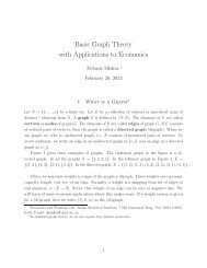
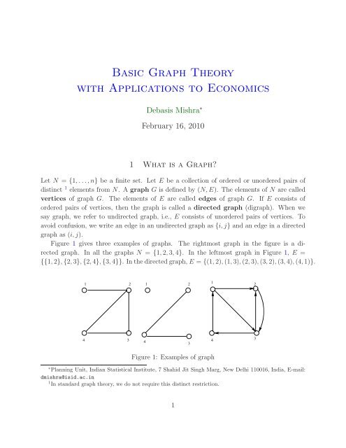
Figure 1 gives three examples of graphs. The rightmost graph in the figure is a directed 

graph. In all the graphs N = {1, 2, 3, 4}. In the leftmost graph in Figure 1, E = 

{{1, 2}, {2, 3}, {2, 4}, {3, 4}}. In the directed graph, E = {(1, 2), (1, 3), (2, 3), (3, 2), (3, 4), (4,1)}. 

1 2 

1 2 

1 

2 

4 

3 

4 

3 

4 

3 

Figure 1: Examples of graph 

∗ Planning Unit, Indian Statistical Institute, 7 Shahid Jit Singh Marg, New Delhi 110016, India, E-mail: 

dmishra@isid.ac.in 

1 In standard graph theory, we do not require this distinct restriction. 

1

Often, we associate weights to edges of the graph or digraph. These weights can represent 

capacity, length, cost etc. of an edge. Formally, a weight is a mapping from set of edges to 

real numbers, w : E → R. Notice that weight of an edge can be zero or negative also. We 

will learn of some economic applications where this makes sense. If a weight system is given 

for a (di)graph, then we write (N, E, w) as the (di)graph. 

1.1 Modeling Using Graphs: Examples 

Example 1: Housing/Job Market 

Consider a market of houses (or jobs). Let there be H = {a, b, c, d} houses on a street. 

Suppose B = {1, 2, 3, 4} be the set of potential buyers, each of whom want to buy exactly 

one house. Every buyer i ∈ B is interested in ∅ ≠ H i ⊆ H set of houses. This situation can 

be modeled using a graph. 

Consider a graph with the following set of vertices: N = H ∪ B (note that H ∩ B = ∅). 

The only edges of the graph are of the following form: for every i ∈ B and every j ∈ H i , 

there is an edge between i and j. Graphs of this kind are called bipartite graphs, i.e., a 

graph whose vertex set can be partitioned into two non-empty sets and the edges are only 

between vertices which lie in separate partitions. 

Figure 2 is a bipartite graph of this example. Here, H 1 = {a}, H 2 = {a, c}, H 3 = 

{b, d}, H 4 = {c}. Is it possible to allocate a unique house to every buyer? 

1 

a 

2 

b 

3 

c 

4 

d 

Figure 2: A bipartite graph 

If every buyer associates a value for every house, then it can be used as a weight of the 

graph. Formally, if there is an edge (i, j) then w(i, j) denotes the value of buyer i ∈ B for 

house j ∈ H i . 

2

Example 2: Coauthor/Social Networking Model 

Consider a model with researchers (or agents in Facebook site). Each researcher wants 

to collaborate with some set of other researchers. But a collaboration is made only if both 

agents (researchers) put substantial effort. The effort level of agent i for edge (i, j) is given 

by w(i, j). 

This situation can be modeled as a directed graph with weight of edge (i, j) being w(i, j). 

Common question here: if there is some utility function of every researcher, in equilibrium 

what kind of graphs will be formed with what weights? 

Example 3: Transportation Networks 

Consider a reservoir located in a state. The water from the reservoir needs to be supplied 

to various cities. It can be supplied directly from the reservoir or via another cities. The 

cost of supplying water from city i to city j is given and so is the cost of supplying directly 

from reservoir to a city. What is the best way to connect the cities to the reservoir? How 

should the cost of connection be split amongst the cities? 

The situation can be modeled using directed or undirected graphs, depending on whether 

the cost matrix is asymmetric or symmetric. The set of nodes in the graph is the set of cities 

and the reservoir. The set of edges is the set of edges from reservoir to the cities and all 

possible edges between cities. The edges can be directed or undirected. For example, if the 

cities are located at different altitudes, then cost of transporting from i to j may be different 

from that from j to i, in which case we model it as a directed graph, else as an undirected 

graph. 

2 Definitions of (Undirected) Graphs 

If {i, j} ∈ E, then i and j are called end points of this edge. The degree of a vertex is 

the number of edges for which that vertex is an end point. So, for every i ∈ N, we have 

deg(i) = #{j ∈ N : {i, j} ∈ E}. In Figure 1, degree of vertex 2 is 3. Here is a simple lemma 

about degree of a vertex. 

Lemma 1 The number of vertices of odd degree is even. 

Proof : Let O be the set of vertices of odd degree. Notice that if we sum of the degrees of 

every vertex, we will count the number of edges exactly twice. Hence, ∑ i∈N 

deg(i) = 2#E. 

Now, ∑ i∈N deg(i) = ∑ i∈O deg(i) + ∑ i∈N\O 

deg(i). Hence, we can write, 

∑ 

deg(i) = 2#E − ∑ 

deg(i). 

i∈O 

i∈N\O 

3

Now, right side of the above equation is even. This is because 2#E is even and for every 

i ∈ N \ O, deg(i) is even by definition. Hence, left side of the above equation ∑ i∈O 

deg(i) is 

even. But for every i ∈ O, deg(i) is odd by definition. Hence, #O must be even. 

A path is a sequence of distinct vertices (i 1 , . . .,i k ) such that {i j , i j+1 } ∈ E for all 

1 ≤ j < k. The path (i 1 , . . .,i k ) is called a path from i 1 to i k . A graph is connected if there 

is a path between every pair of vertices. The middle graph in Figure 1 is not connected. 

A cycle is a sequence of vertices (i 1 , . . .,i k , i k+1 ) with k > 2 such that {i j , i j+1 } ∈ E for 

all 1 ≤ j ≤ k, (i 1 , . . .,i k ) is a path, and i 1 = i k+1 . In the leftmost graph in Figure 1, a path 

is (1, 2, 3) and a cycle is (2, 3, 4, 2). 

A graph G ′ = (N ′ , E ′ ) is a subgraph of graph G = (N, E) if ∅ ≠ N ′ ⊆ N, E ′ ⊆ E, and 

for every {i, j} ∈ E ′ we have i, j ∈ N ′ . A connected acyclic (that does not contain a cycle) 

graph is called a tree. Graphs in Figure 1 are not trees, but the second and third graph 

in Figure 3 are trees. A graph may contain several trees (i.e. connected acyclic subgraphs). 

The spanning tree of a connected graph is a subgraph (N, E ′ ) such that (N, E ′ ) is a tree. 

Note that E ′ ⊆ E and a spanning tree does not contain a cycle. By definition, every tree 

(N ′ , E ′ ) is a spanning tree of graph (N ′ , E ′ ). 

Figure 3 shows a connected graph (which is not a tree) and two of its spanning trees. 

4 

4 

4 

1 

1 

1 

2 3 

2 3 

2 3 

Figure 3: Spanning trees of a graph 

2.1 Properties of Trees and Spanning Trees 

We now prove some properties of trees and spanning trees. 

Proposition 1 Every tree G ′ = (N ′ , E ′ ), where G ′ is a subgraph of a graph G = (N, E), 

satisfies the following properties. 

1. There is a unique path from i to j in G ′ for every i, j ∈ N ′ . 

2. If there is an edge {i, j} ∈ E \ E ′ with i, j ∈ N ′ , adding {i, j} to E ′ creates a cycle. 

4

3. By removing an edge from E ′ disconnects the tree. 

4. Every tree with at least two vertices has at least two vertices of degree one. 

5. #E ′ = #N ′ − 1. 

Proof : 

1. Suppose there are at least two paths from i to j. Let these two paths be P 1 = 

(i, i 1 , . . ., i k , j) and P 2 = (i, j 1 , . . .,j q , j). Then, consider the following sequence of 

vertices: (i, i 1 , . . .,i k , j, j q , . . .,j 1 , i). This sequence of vertices is a cycle or contains a 

cycle if both paths share edges, contradicting the fact that G ′ is a tree. 

2. Consider an edge {i, j} ∈ E \ E ′ (if no such edge exists, then we are vacuously done). 

In graph G ′ , there was a unique path from i to j. The edge {i, j} introduces another 

path. This means the graph G ′′ = (N ′ , E ′ ∪ {i, j}) is not a tree (from the claim above). 

Since G ′′ is connected, it must contain a cycle. 

3. Let {i, j} ∈ E ′ be the edge removed from G ′ . By the first claim, there is a unique path 

from i to j in G ′ . Since there is an edge between i and j, this unique path is the edge 

{i, j}. This means by removing this edge we do not have a path from i to j, and hence 

the graph is no more connected. 

4. We do this using induction on number of vertices. If there are two vertices, the claim 

is obvious. Consider a tree with n vertices. Suppose the claim is true for any tree 

with < n vertices. Now, consider any edge {i, j} in the tree. By (1), the unique path 

between i and j is this edge {i, j}. Now, remove this edge from the tree. By (3), we 

disconnect the tree into trees which has smaller number of vertices. Each of these trees 

have either a single vertex or have two vertices with degree one (by induction). By 

connecting edge {i, j}, we can increase the degree of one of the vertices in each of these 

trees. Hence, there is at least two vertices with degree one in the original graph. 

5. For #N ′ = 2, it is obvious. Suppose the claim holds for every #N ′ = m. Now, consider 

a tree with (m + 1) vertices. By the previous claim, there is a vertex i that has degree 

1. Let the edge for which i is an endpoint be {i, j}. By removing i, we get another 

tree of subgraph (N ′ \ {i}, E ′ \ {i, j}). By induction, number of edges of this tree is 

m − 1. Since, we have removed one edge from the original tree, the number of edges 

in the original tree (of a graph with (m + 1) vertices) is m. 

We prove two more important, but straightforward, lemmas. 

 

5

Lemma 2 Let G = (N, E) be a graph and G ′ = (N, E ′ ) be a subgraph of G such that 

#E ′ = #N − 1. If G ′ has no cycles then it is a spanning tree. 

Proof : Call a subgraph of a graph G a component of G if it is maximally conntected, i.e., 

G ′′ = (N ′′ , E ′′ ) is a component of G = (N, E) if G ′′ is connected and there does not exist 

vertices i ∈ N ′′ and j ∈ N \ N ′′ such that {i, j} ∈ E. 

Clearly, any graph can be partitioned into its components with a connected graph having 

one component, which is the same graph. Now, consider a graph G = (N, E) and let 

G 1 , . . .,G q be the components of G with number of vertices in component G j being n j for 

1 ≤ j ≤ q. Since every component is a tree, by Proposition 1 the number of edges in 

component G j is n j − 1 for 1 ≤ j ≤ q. Since the components have no vertices and edges in 

common, the total number of edges in components G 1 , . . .,G q is 

(n 1 − 1) + . . . + (n q − 1) = (n 1 + n 2 + . . . + n q ) − q = #N − q. 

By our assumption in the claim, the number of edges in G is #N −1. Hence, q = 1, i.e., the 

graph G is a component, and hence a spanning tree. 

 

Lemma 3 Let G = (N, E) be a graph and G ′ = (N, E ′ ) be a subgraph of G such that 

#E ′ = #N − 1. If G ′ is connected, then it is a spanning tree. 

Proof : We show that G ′ has no cycles, and this will show that G ′ is a spanning tree. We 

do the proof by induction on #N. The claim holds for #N = 2 and #N = 3 trivially. 

Consider #N = n > 3. Suppose the claim holds for all graphs with #N < n. In graph 

G ′ = (N, E ′ ), there must be a vertex with degree 1. Else, every vertex has degree at least two 

(it cannot have degree zero since it is connected). In that case, the total degree of all vertices 

is 2#E ≥ 2n or #E = n −1 ≥ n, which is a contradiction. Let this vertex be i and let {i, j} 

be the unique edge for which i is an endpoint. Consider the graph G ′′ = (N \{i}, E ′ \{{i, j}}). 

Clearly, G ′′ is connected and number of edges in G ′′ is one less than n − 1, which equals the 

number of edges in E ′ \ {{i, j}}. By our induction hypothesis, G ′′ has no cycles. Hence, G ′ 

cannot have any cycle. 

 

3 The Minimum Cost Spanning Tree Problem 

Consider a graph G = (N, E, w), i.e., a weighted graph. Assume G to be connected. Imagine 

the weights to be costs of traversing an edge. So, w ∈ R #E 

+ . The minimum cost spanning 

tree (MCST) problem is to find a spanning tree of minimum cost in graph G. Figure 4 

shows a weighted graph. In this figure, one can imagine one of the vertices as “source” (of 

water) and other vertices to be cities. The weights on edges may represent cost of supplying 

6

a 

2 

b 

1 

2 

3 

1 

d 

4 

c 

Figure 4: The minimum cost spanning tree problem 

water from one city to another. In that case, the MCST problem is to find a minimum cost 

arrangement (spanning tree) to supply water to cities. 

There are many greedy algorithms that find an MCST. We give a generic algorithm, and 

show one specific algorithm that falls in this generic class. 

The generic greedy algorithm grows an MCST one edge at a time. The algorithm manages 

a subset A of edges that is always a subset of some MCST. At each step of the algorithm, an 

edge {i, j} is added to A such that A ∪ {{i, j}} is a subset of some MCST. We call such an 

edge a safe edge for A (since it can be safely added to A without destroying the invariant). 

In Figure 4, A can be taken to be {{b, d}, {a, d}}, which is a subset of an MCST. A safe edge 

for A is {a, c}. 

Here is the formal procedure: 

1. Set A = ∅. 

2. If (N, A) is not a spanning tree, then find an edge {i, j} that is safe for A. Set 

A ← A ∪ {{i, j}} and repeat from Step 2. 

3. If (N, A) is a spanning tree, then return (N, A). 

Remark: After Step 1, the invariant (that in every step we maintain a set of edges which 

belong to some MCST) is trivially satisfied. Also, if A is not a spanning tree but a subset of 

an MCST, then there must exist an edge which is safe. 

The question is how to identify safe edges. We discuss one such rule. The algorithm we 

discuss is due to Kruskal, and hence called the Kruskal’s algorithm. For this, we provide 

some definitions. A cut in a graph G = (N, E) is a partition of set of vertices (V, N \ V ) 

with V ≠ N and V ≠ ∅. An edge {i, j} crosses a cut (V, N \V ) if i ∈ V and j ∈ N \V . We 

say a cut (V, N \ V ) respects a set of edges A if no edge from A crosses the cut. A light 

7

edge crossing a cut (V, N \ V ) is an edge that has the minimum weight among all the edges 

crossing the cut (V, N \ V ). 

Figure 5 shows a graph and two of its cuts. The first cut is ({1, 2, 3}, {4, 5, 6}). The 

following set of edges respect this cut {{1, 2}, {1, 3}}. Also, the set of edges {{4, 5}, {5, 6}} 

and the set of edges {{1, 3}, {4, 5}} respect this cut. Edges {1, 4}, {2, 6}, {3, 4} cross this 

cut. 

1 

4 

1 

4 

5 

3 

5 

3 

2 

6 

2 

6 

Figure 5: Cuts in a graph 

The following theorem says how a light edge of an appropriate cut is a safe edge. 

Theorem 1 Let G = (N, E, w) be a connected graph. Let A ⊂ T ⊆ E be a subset of edges 

such that (N, T) is an MCST of G. Let (V, N \ V ) be any cut of G that respects A and let 

{i, j} be a light edge crossing (V, N \ V ). Then edge {i, j} is a safe edge for A. 

Proof : Let A be a subset of edges of MCST (N, T). If {i, j} ∈ T, then we are done. So, 

we consider the case when {i, j} /∈ T. Since (N, T) is a spanning tree, adding edge {i, j} 

to T creates a cycle (Proposition 1). Hence, the sequence of vertices in the set of edges 

T ∪ {{i, j}} contains a cycle between vertex i and j (this is the only cycle). This cycle 

must cross the cut (V, N \ V ) at least twice - once at {i, j} and the other at some edge 

{a, b} ≠ {i, j} such that a ∈ V , b ∈ N \ V which crosses the cut (V, N \ V ). Note that 

{a, b} ∈ T. If we remove edge {a, b}, then this cycle is broken and we have no cycle in the 

graph G ′′ = (N, (T ∪ {{i, j}}) \ {{a, b}}). By Proposition 1, there are #N − 1 edges in 

(N, T). Hence, G ′′ also has #N − 1 edges. By Lemma 2, G ′′ is a spanning tree. 

Let T ′ = (T ∪{{i, j}})\{{a, b}}. Now, the difference of edge weights of T and T ′ is equal to 

w({a, b})−w({i, j}). Since (N, T) is an MCST, we know that w({a, b})−w({i, j}) ≤ 0. Since 

{i, j} is a light edge of cut (V, N \V ) and {a, b} crosses this cut, we have w({a, b}) ≥ w({i, j}). 

Hence, w({a, b}) = w({i, j}). Hence (N, T ′ ) is an MCST. 

This proves that (A ∪ {{i, j}}) ⊆ T ′ . Hence, {i, j} is safe for A. 

 

8

The above theorem almost suggests an algorithm to compute an MCST. Consider the 

following algorithm. Denote by V (A) the set of vertices which are endpoints of edges in A. 

1. Set A = ∅. 

2. Choose any vertex i ∈ N and consider the cut ({i}, N \ {i}). Let {i, j} be a light edge 

of this cut. Then set A ← A ∪ {{i, j}}. 

3. If A contains #N − 1 edges then return A and stop. Else, go to Step 4. 

4. Consider the cut (V (A), N \ V (A)). Let {i, j} be a light edge of this cut. 

5. Set A ← A ∪ {{i, j}} and repeat from Step 3. 

This algorithm produces an MCST. To see this, by Theorem 1, in every step of the 

algorithm, we add an edge which is safe. This means the output of the algorithm contains 

#N − 1 edges and no cycles. By Lemma 2, this is a spanning tree. By Theorem 1, this is 

an MCST. 

We apply this algorithm to the example in Figure 4. In the first iteration of the algorithm, 

we choose vertex a and consider the cut ({a}, {b, c, d}). A light edge of this cut is {a, c}. So, 

we set A = {{a, c}}. Then, we consider the cut ({a, c}, {b, d}). A light edge of this cut is 

{a, d}. Now, we set A = {{a, c}, {a, d}}. Then, we consider the cut ({a, c, d}, {b}). A light 

edge of this cut is {b, d}. Since (N, {a, c}, {a, d}, {b, d}) is a spanning tree, we stop. The 

total weight of this spanning tree is 1 + 2 + 1 = 4, which gives the minimum weight over all 

spanning trees. Hence, it is an MCST. 

4 Application: The Minimum Cost Spanning Tree Game 

In this section, we define a coopearative game corresponding to the MCST problem. To do 

so, we first define the notion of a cooperative game and a well known stability condition for 

such games. 

4.1 Cooperative Games 

Let N be the set of agents. A subset S ⊆ N of agents is called a coalition. Let Ω be the set 

of all coalitions. A cooperative game is a tuple (N, c) where N is a finite set of agents and 

c is a characteristic function defined over set of coalitions Ω, i.e., c : Ω → R. The number 

c(S) can be thought to be the cost incurred by coalition S when they cooperate 2 . 

2 Cooperative games can be defined with value functions also, in which case notations will change, but 

ideas remain the same. 

9

The problem is to divide the total cost c(N) amongst the agents in N when they cooperate. 

We give an example of a cooperative game and analyze it below. Before that, we 

describe a well known solution concept of core. 

A cost vector x assigns every player a cost in a game (N, c). The core of a cooperative 

game (N, c) is the set of cost vectors which satisfies a stability condition. 

Core(N, c) = {x ∈ R #N : ∑ i∈N 

x i = c(N), 

∑ 

x i ≤ c(S) ∀ S N} 

i∈S 

Every cost vector in the core is such that it distributes the total cost c(N) amongst agents 

in N and no coalition of agents can be better off by forming their independent coalition. 

There can be many cost vectors in a core or there may be none. For example, look at 

the following game with N = {1, 2}. Let c(12) = 5 and c(1) = c(2) = 2. Core conditions 

tell us x 1 ≤ 2 and x 2 ≤ 2 but x 1 + x 2 = 5. But there are certain class of games which have 

non-empty core (more on this later). We discuss one such game. 

4.2 The Minimum Cost Spanning Tree Game 

The minimum cost spanning tree game (MCST game) is defined by set of agents N = 

{1, . . ., n} and a source agent to whom all the agents in N need to be connected. The 

underlying graph is (N ∪ {0}, E, c) where E = {{i, j} : i, j ∈ N ∪ {0}, i ≠ j} and c(i, j) 

denotes the cost of edge {i, j}. For any S ⊆ N, let S + = S ∪ {0}. When a coalition of 

agents S connect to source, they form an MCST using edges between themseleves. Let c(S) 

be the total cost of an MCST when agents in S form an MCST with the source. Thus, (N, c) 

defines a cooperative game. 

An example is given in Figure 6. Here N = {1, 2, 3} and c(123) = 4, c(12) = 4, c(13) = 

3, c(23) = 4, c(1) = 2, c(2) = 3, c(3) = 4. It can be verified that x 1 = 2, x 2 = 1 = x 3 is in the 

core. The next theorem shows that this is always the case. 

For any MCST (N, T), let {p(i), i} be the last edge in the unique path from 0 to agent i. 

Define x i = c(p(i), i) for all i ∈ N. Call this the Bird allocation - named after the inventor 

of this allocation. 

Theorem 2 Any Bird allocation is in the core of the MCST game. 

Proof : For any Bird allocation x, by definition ∑ i∈N x i = c(N). Consider any coalition 

S N. Assume for contradiction c(S) < ∑ i∈S x i. Then, consider the MCST corresponding 

to nodes S + (which only use edges having endpoints in S + ). Such an MCST has #S edges 

by Proposition 1. Add the edges of this tree to the MCST corresponding to nodes N + . The, 

delete for every i ∈ S, the edge e i = {p(i), i} from this new graph. Let this graph be (N, T ′ ). 

10

1 

2 

1 2 

0 

4 

3 

3 

1 

2 

Figure 6: An MCST game 

Note that (N, T ′ ) has the same number (#N − 1) edges as the MCST corresponding to N + . 

We show that (N, T ′ ) is connected. It is enough to show that there is a path from source to 

every vertex i ∈ N. We consider two cases. 

Case 1: Consider any vertex i ∈ S. We have a path from 0 to i in (N, T ′ ) by the MCST 

corresponding S + . 

Case 2: Consider any vertex i /∈ S. Take the path in the MCST corresponding to N + from 

0 to i and let j be the last vertex such that j ∈ S. In (N, T ′ ), we can take 0 to j path in 

MCST corresponding to S + and continue on the remaining path in the path from 0 to i in 

the MCST corresponding to N + . 

This shows that (N, T ′ ) is connected and has #N − 1 edges. By Lemma 3, (N, T ′ ) is a 

spanning tree. 

Now, the new spanning tree has cost c(N) − ∑ i∈S x i +c(S) < c(N) by assumption. This 

violates the fact that the original tree is an MCST. 

 

5 Hall’s Marriage Theorem 

Consider a society with a finite set of boys B and a finite set of girls L with #L ≤ #B. 

We want to find if boys and girls can married in a compatible manner. For every girl 

i ∈ L, a set of boys ∅ ≠ B i are compatible. We say girl i likes boy j if and only if 

j ∈ B i . This can be represented as a bipartite graph with vertex set B ∪ L and edge set 

E = {{i, j} : i ∈ L, j ∈ B i }. We will denote such a bipartite graph as G = (B ∪ L, {B i } i∈L ). 

We say two edges {i, j}, {i ′ , j ′ } in a graph are disjoint if i, j, i ′ , j ′ are all distinct, i.e., 

the endpoints of the edges are distinct. A set of edges are disjoint if every pair of edges in 

11

that set are disjoint. A matching in graph G is a set of edges which are disjoint. We ask 

whether there exists a matching with #L edges. 

Figure 7 shows a bipartite graph with a matching: {{1, b}, {2, a}, {3, d}, {4, c}}. 

1 

a 

2 

b 

3 

c 

4 

d 

Figure 7: A bipartite graph with a matching 

Clearly, a matching will not always exist. Consider the case where #L ≥ 2 and for every 

i ∈ L, we have B i = {j} for some j ∈ B, i.e, every girl likes the same boy - j. No matching 

is possible in this case. 

In general, if we take a subset S ⊆ L of girls and take the set of boys that girls in S like: 

D(S) = ∪ i∈S B i , then #S ≤ #D(S) is necessary for a matching to exist. Else, number of 

boys who girls in S like are less, and so some girl cannot be matched. For example, if we 

pick a set of 5 girls who like only a set of 3 boys, then we cannot match some girls. 

Hall’s marriage theorem states that this condition is also sufficient. 

Theorem 3 A matching with #L edges in a bipartite graph G = (B ∪ L, {B i } i∈L ) exists if 

and only if for every ∅ ≠ S ⊆ L, we have #S ≤ #D(S), where D(S) = ∪ i∈S B i . 

Proof : Suppose a matching with #L edges exists in G. Then, we have #L disjoint edges. 

Denote this set of edges as M. By definition, every edge in M has a unique girl and a 

unique boy as endpoints, and for every {i, j} ∈ M we have j ∈ B i . Now, for any set of girls 

∅ ≠ S ⊆ L, we define M(S) = {j ∈ B : {i, j} ∈ M, i ∈ S} - the set of boys matched to girls 

in S in matching M. We know that #S = #M(S). By definition M(S) ⊆ D(S). Hence 

#S ≤ #D(S). 

Suppose for every ∅ ≠ S ⊆ L, we have #S ≤ #D(S). We use induction to prove that a 

matching with #L edges exists. If #L = 1, then we just match her to one of the boys she 

likes (by our condition she must like at least one boy). Suppose a matching with #L edges 

exists for any society with less than l +1 girls. We will show that a matching with #L edges 

exists for any society with #L = l + 1 girls. 

There are two cases to consider. 

Case 1: Suppose #S < #D(S) for every ∅ ≠ S ⊂ L (notice proper subset). Then choose 

an arbitrary girl i ∈ L and any j ∈ B i , and consider the edge {i, j}. Now consider the 

12

ipartite graph G ′ = (B \ {j} ∪ L \ {i}, {B k \ {j}} k∈L\{i} ). Now, G ′ is a graph with l girls. 

Since we have removed one boy and one girl from G to form G ′ and since #S ≤ #D(S) − 1 

for all ∅ ≠ S ⊂ L, we will satisfy the condition in the theorem for graph G ′ . By induction 

assumption, a matching exists in graph G ′ with #L − 1 edges. This matching along with 

edge {i, j} forms a matching of graph G with #L edges. 

Case 2: For some ∅ ≠ S ⊂ L, we have #S = #D(S). By definition #S < #L, and hence 

by induction we have a matching in the graph G ′ = (S ∪ D(S), {B i } i∈S ) with #S edges. 

Now consider the graph G ′′ = ((B \ D(S)) ∪ (L \ S), {B i \ D(S)} i∈L\S ). We will show that 

the condition in the theorem holds in graph G ′′ . Consider any ∅ ≠ T ⊆ (L \ S). Define 

D ′ (T) = D(T) \ D(S). We have to show that #T ≤ #D ′ (T). We know that #(T ∪ S) ≤ 

#D(T ∪ S). We can write #D(T ∪ S) = #D(S) + #(D(T) \ D(S)) = #D(S) + #D ′ (T). 

Hence, #(T ∪S) = #T+#S ≤ #D(S)+#D ′ (T). But #S = #D(S). Hence, #T ≤ #D ′ (T). 

Hence, the condition in the theorem holds for graph G ′′ . By definition #(L \ S) < #L. So, 

we apply the induction assumption to find a matching in G ′′ with #(L \ S) edges. Clearly, 

the matchings of G ′ and G ′′ do not have common edges, and they can be combined to get a 

matching of G with #L edges. 

 

Remark: Hall’s marriage theorem tells you when a matching can exist in a bipartite graph. 

It is silent on the problem of finding a matching when it exists. We will study other results 

about existence and feasibility later. 

5.1 Application: Competitive Markets with Indivisible Goods 

The matching literature in economics in long. I will illustrate a use of Hall’s theorem to an 

economics setting. 

Consider a market with a set of indivisible goods (like houses, cars etc.) and a set of 

buyers each of whom want to buy exactly one good. The set of indivisible goods is denoted by 

N = {1, . . ., n} and set of buyers is denoted by M = {1, . . .,m}. Assume m ≤ n. The seller 

of the goods announce prices for the goods, denoted by a price vector p ∈ R n + . Buyers report 

their demand at the price vector p. The demand of buyer i ∈ M at price vector p is denoted 

as D p i . This model can be represented using a bipartite graph G = (M ∪ N, {Dp i } i∈M). We 

say the price vector p is competitive if a matching exists in G with m edges. Note that a 

matching may leave some goods unmatched to any buyer. The question is how to verify if a 

price vector is competitive. 

Define the exclusive demanders of a set of goods ∅ ≠ S ⊆ N at price vector p as 

O p (S) = {i ∈ M : D p i ⊆ S}. As an example, consider M = {1, 2, 3} and N = {1, 2, 3, 4} and 

for some price vector p, D p 1 = {1, 2}, D p 2 = {2, 3}, D p 3 = {2, 4}. Now, exclusive demanders 

of {1, 2, 3} are {1, 2}. A set of goods ∅ ≠ S ⊆ N is overdemanded at price vector p if 

#S < #O p (S). 

13

Theorem 4 A price vector is competitive if and only if no set of goods is overdemanded at 

that price vector. 

Proof : By definition, a price vector is competitive if and only if a matching exists in the 

bipartite graph G = (M ∪ N, {D p i } i∈M). One side of the proof is obvious. If we have an 

overdemanded set of goods, say S, then #O p (S) > #S. This means, we cannot match buyers 

in O p (S). Hence, if a price vector is competitive then no set of goods is overdemanded. 

The other direction of the proof is a straightforward application of Hall’s marriage theorem. 

Suppose no set of goods is overdemanded. Now, consider a set of buyers ∅ ≠ B ⊆ M. 

Let S = ∪ i∈B D p i . Notice that B ⊆ Op (S). Since S is not overdemanded, we get #S ≥ 

#O p (S) ≥ #B. Hence #B ≤ #S. By Hall’s marriage theorem (Theorem 3), there exists a 

matching in graph G with m edges. 

 

6 Maximum Matching in Bipartite Graph 

We saw in the last section that matching all girls in a bipartite matching problem requires 

a combinatorial condition hold. In this section, we ask the question - what is the maximum 

number of matchings that is possible in a bipartite graph? We will also discuss an algorithm 

to compute such a maximum matching. 

6.1 M-Augmenting Path 

We start with the notion of augmenting path in an arbitrary undirected graphs. To remind, 

in a graph G = (N, E), a matching M ⊆ E is a set of disjoint edges in G. Here, one can 

think of nodes in G to be students, the set of edges to be set of possible pairings of students. 

The problem of finding roommates for students can be thought to be a problem of finding a 

matching (of maximum size) in G. Figures 8 and 9 show two matchings in a graph - dark 

edges represent a matching. 

Before we introduce the definition of an augmenting path, we introduce some terminology. 

The length of a path (cycle) is the number of edges in a path (cycle). Given a graph 

G = (N, E), a set of vertices S ⊆ N is covered by a set of edges X ⊆ E if every vertex in 

S is an endpoint of some edge in X. 

Definition 1 Let M be a matching in a graph G = (N, E). A path P (with non-zero 

length) in G is called M-augmenting if its ends are not covered by M and its edges are 

alternatingly out of and in M. 

Note that an M-augmented path need not contain all the edges in M. Since an M- 

augmenting path has odd number of edges, the number of edges in M is less than the 

14

2 

3 

4 

1 

6 

5 

Figure 8: A matching in a graph 

2 

3 

4 

1 

6 

5 

Figure 9: A matching in a graph 

number of edges out of M in an M-augmenting path. An M-augmenting path may contain 

a single edge also. 

Figures 10 and 11 show two matchings and their respective M-augmenting paths. 

2 

3 

4 

1 

6 

5 

Figure 10: An M-augmenting path for a matching 

Definition 2 A matching M in graph G = (N, E) is maximum if there does not exist 

another matching M ′ in G such that #M ′ > #M. 

It can be verified that the matching in Figure 8 is a maximum matching. There is 

an obvious connection between maximum matchings and augmenting paths. For example, 

15

2 

3 

4 

1 

6 

5 

Figure 11: An M-augmenting path for a matching 

notice the maximum matching M in Figure 8. We cannot seem to find an M-augmenting 

path for this matching. On the other hand, observe that the matching in Figure 9 is not 

a maximum matching (the matching in Figure 8 has more edges), and Figure 10 shows an 

augmenting path of this matching. This observation is formalized in the theorem below. 

Theorem 5 Let G = (N, E) be a graph and M be a matching in G. Then, either M is a 

maximum matching or there exists an M-augmenting path. 

Proof : Suppose M is a maximum matching. Assume for contradiction that P is an M- 

augmenting path. Let E P be the set of edges in P. Now define, M ′ = (E P \M) ∪(M \E P ). 

By definition of an augmenting path, E P \M contains more edges than E P ∩M. Hence, M ′ 

contains more edges than M. Also, by definition of an augmenting path, the edges in E P \M 

are disjoint. Since M is a matching, the set of edges in (M \ E P ) are disjoint. Also, by the 

definition of the augmenting path (ends of an augmenting path are not covered in M), we 

have that the edges in (E P \M) and edges in (M \E P ) cannot share an endpoint. Hence, M ′ 

is a set of disjoint edges, i.e., a matching with size larger than M. This is a contradiction. 

Now, suppose M is not a maximum matching and there is another matching M ′ larger 

than M. Consider the graph G ′ = (N, M ∪ M ′ ). Hence, every vertex of graph G ′ has degree 

in {0, 1, 2}. Now, partition G ′ into components. Each component has to be either an isolated 

vertex or a path or a cycle. Note that every cycle must contain equal number of edges from 

M and M ′ . Since the number of edges in M ′ is larger than that in M, there must exist 

a component of G ′ which is a path and which contains more edges from M ′ than from M. 

Such a path forms an M-augmenting path (Think why this is true). 

 

Theorem 5 suggests a simple algorithm for finding a maximum matching. The algorithm 

starts from some arbitrary matching, may be the empty one. Then, it searches for an 

augmenting path of this matching. If there is none, then we have found a maximum matching, 

else the augmenting path gives us a matching larger than the current matching, and we 

repeat. Hence, as long as we can find an augmenting path for a matching, we can find a 

16

maximum matching. Before we give an algorithm to find an augmenting path, we present a 

useful result. 

6.2 Minimum Vertex Cover and Maximum Matching 

The size of a maximum matching in a graph is the number of edges in the maximum 

matching. We define vertex cover now and show its relation to matching. In particular, we 

show that the minimum vertex cover and the maximum matching of a bipartite graph have 

the same size. 

Definition 3 Give a graph G = (N, E), a set of vertices C ⊆ N is called a vertex cover 

of G if every edge in E has at least one end point in C. Further, C is called a minimum 

vertex cover of G if there does not exist another vertex cover C ′ of G such that #C ′ < #C. 

Clearly, the set of all vertices in a graph consists of a vertex cover. But this may not be 

a minimum vertex cover. We give some examples in Figure 12. Figure 12 shows two vertex 

covers of the same graph - vertex covers are shown with black vertices. The first one is not 

a minimum vertex cover but the second one is. 

2 

3 

2 

3 

1 

4 

1 

4 

6 

5 

6 

5 

Figure 12: Vertex cover 

An application of the vertex cover can be as follows. Suppose the graph represents a 

city: the vertices are squares and the edges represent streets. The city plans to deploy 

security office (or medical store or emergency service or park) at squares to monitor streets. 

A security officer deployed at a square can monitor all streets which have an endpoint in 

that square. The minimum vertex cover problem finds the minimum set of squares where 

one needs to put a security officer to monitor all the streets. 

Fix a graph G. Denote the size of maximum matching in G as ν(G) - this is also called 

the matching number of G. Denote the size of minimum cover in G as τ(G) - this is also 

called the vertex cover number of G. 

Lemma 4 For any graph G, ν(G) ≤ τ(G). 

17

Proof : Any vertex cover contains at least one end point of every edge of a matching. Hence, 

consider the maximum matching. A vertex cover will contain at least one vertex from every 

edge of this matching. This implies that for every graph G, ν(G) ≤ τ(G). 

Lemma 4 can hold with strict inequality in general graphs. Consider the graph in Figure 

13. A minimum vertex cover, as shown with black vertices, has two vertices. A maximum 

matching, as shown with the dashed edge, has one edge. 

1 

2 3 

Figure 13: Matching number and vertex cover number 

But the relationship in Lemma 4 is equality in case of bipartite graphs as the following 

theorem, due to Ko¨nig shows. 

Theorem 6 (Ko¨nig’s Theorem) Suppose G = (N, E) is a bipartite graph. Then, ν(G) = 

τ(G). 

1 

a 

2 

b 

3 

c 

4 

d 

Figure 14: Matching number and vertex cover number in bipartite graphs 

Figure 14 shows a bipartite graph and its maximum matching edges (in dark) and minimum 

vertex cover (in dark). For the bipartite graph in Figure 14 the matching number (and 

the vertex cover number) is two. 

18

We will require the following useful result for proving Theorem 6. A graph may have 

multiple maximum matchings. The following result says that there is at least one vertex 

which is covered by every maximum matching if the graph is bipartite. 

Lemma 5 Suppose G = (N, E) is a bipartite graph with E ≠ ∅. Then, there exists a vertex 

in G which is covered by every maximum matching. 

Proof : Assume for contradiction that every vertex is not covered by some maximum matching. 

Consider any edge {i, j} ∈ E. Suppose i is not covered by maximum matching M and 

j is not covered by maximum matching M ′ . Note that j must be covered by M - else adding 

{i, j} to M gives another matching which is larger in size than M. Similarly, i must be 

covered by M ′ . Note that the edge {i, j} is not in (M ∪ M ′ ). 

Consider the graph G ′ = (N, M ∪ M ′ ). A component of G ′ must contain i (since M ′ 

covers i). Such a component will have alternating edges in and out of M and M ′ . Since i 

is covered by M ′ and not by M, i must be an end point in this component. Further, this 

component must be a path - denote this path by P. Note that P contains alternating edges 

from M and M ′ (not in M). The other endpoint of P must be a vertex k which is covered by 

M - else, P defines an M-augmenting path, contradicting that M is a maximum matching 

by Theorem 5. This also implies that k is not covered by M ′ and P has even number of 

edges. 

We argue that P does not contain j. Suppose P contains j. Since j is covered by M and 

not by M ′ , j must be an endpoint of P. Since G is bipartite, let N = B ∪ L and every edge 

{u, v} ∈ E is such that u ∈ B and v ∈ L. Suppose i ∈ B. Since the number of edges in P is 

even, both the end points of P must be in B. This implies that j ∈ B. This contradicts the 

fact that {i, j} is an edge in G. 

So, we conclude that j is not in P. Consider the path P ′ formed by adding edge {i, j} 

to P. This means j is an end point of P ′ . Note that j is not covered by M ′ and the other 

endpoint k of P ′ is also not covered by M ′ . We have alternating edges in and out of M ′ in 

P ′ . Hence, P ′ defines an M ′ -augmenting path. This is a contradiction by Theorem 5 since 

M ′ is a maximum matching. 

 

Proof of Theorem 6 

Proof : We use induction on number of vertices in G. The theorem is clearly true if G has 

one or two vertices. Suppose the theorem holds for any bipartite graph with less than n 

vertices. Let G = (N, E) be a bipartite graph with n vertices. By Lemma 5, there must 

exist a vertex i ∈ N such that every maximum matching of G must cover i. Let E i be the 

set of edges in G for which i is an endpoint. Consider the graph G ′ = (N \ {i}, E \E i ). Note 

that G ′ is bipartite and contains one less vertex. Hence, ν(G ′ ) = τ(G ′ ). 

19

We show that ν(G ′ ) = ν(G) − 1. By deleting the edge covering i in any maximum 

matching of G, we get a matching of G ′ . Hence, ν(G ′ ) ≥ ν(G)−1. Suppose ν(G ′ ) > ν(G)−1. 

This means, ν(G ′ ) ≥ ν(G). Hence, there exists a maximum matching of G ′ , which is also 

a matching of G, and has as many edges as the maximum matching matching of G. Such 

a maximum matching of G ′ must be a maximum matching of G as well and cannot cover i 

since i is not in G ′ . This is a contradiction since i is a vertex covered by every maximum 

matching of G. 

This shows that ν(G ′ ) = τ(G ′ ) = ν(G) − 1. Consider the minimum vertex cover C of G ′ 

and add i to C. Clearly C ∪ {i} is a vertex cover of G and has τ(G ′ )+1 vertices. Hence, the 

minimum vertex cover of G must have no more than τ(G ′ ) + 1 = ν(G) vertices. This means 

τ(G) ≤ ν(G). But we know from Lemma 4 that τ(G) ≥ ν(G). Hence, τ(G) = ν(G). 

This theorem has several corollaries. We leave the proofs of these corollaries as an exercise. 

A matching of graph G is perfect if it covers all the vertices of G. 

Corollary 1 A bipartite graph G = (N, E) has a perfect matching if and only if each 

vertex cover has size at least 1 2 #N. 

A graph is regular if every vertex has equal degree. 

Corollary 2 Every regular bipartite graph (with positive degree) has a perfect matching. 

6.3 Algorithm for Maximum Matching 

We describe a simple algorithm to find a maximum matching. We have already laid the 

foundation for such an algorithm earlier in Theorem 5, where we proved that any matching 

is either a maximum matching or there exists an augmenting path of that matching which 

gives a larger matching than the existing one. We use this fact. 

The algorithm starts from an arbitrary matching and searches for an augmenting path of 

that matching. Let M be any matching of bipartite graph G = (N, E) and N = B ∪ L such 

that for every {i, j} ∈ E we have i ∈ B and j ∈ L. Given the matching M, we construct a 

directed graph G M from G as follows: 

• The set of vertices of G M is N. 

• For every {i, j} ∈ M with i ∈ B and j ∈ L, we create the edge (i, j) in graph G M , i.e., 

edge from i to j. 

• For every {i, j} /∈ M with i ∈ B and j ∈ L, we create the edge (j, i) in graph G M , i.e., 

edge from j to i. 

20

1 

a 

1 

a 

2 

b 

2 

b 

3 

c 

3 

c 

4 

d 

4 

d 


Consider the bipartite graph in Figure 15 (left one) and the matching M shown with dark 

edges. For the matching M, the corresponding directed graph G M is shown on the right in 

Figure 15. 

Let B M be the set of vertices in B not covered by M and L M be the set of vertices in L 

not covered by M. Note that every vertex in B M has no outgoing edge and every vertex in 

L M has no incoming edge. 

We first prove a useful lemma. For every directed path in G M the corresponding path in 

G is the path obtained by removing the directions of the edges in the path of G M . 

Lemma 6 A path in G is an M-augmenting path if and only if it is the corresponding path 

of a directed path in G M which starts from a vertex in L M and ends at a vertex in B M . 

Proof : Consider a directed path P in G M which starts from a vertex in L M and ends at 

vertex in B M . By definition, the endpoints of P are not covered by M. Since edges from L 

to B are not in M and edges from B to L are in M in G M , alternating edges in P is in and 

out of M. Hence, the corresponding path in G is an M-augmenting path. 

For the converse, consider an M-augmenting path in G and let P be this path in G M 

with edges appropriately oriented. Note that endpoints of P are not covered by M. Hence, 

the starting point of P is in L M and the end point of P is in B M - if the starting point 

belonged to B M , then there will be no outgoing edge and if the end point belonged to L M , 

then there will be no incoming edge. This shows that P is a directed path in G M which 

starts from a vertex in L M and ends at a vertex in B M . 

 

Hence, to find an augmenting path of a matching, we need to find a specific type of path 

in the corresponding directed graph. Consider the matching M shown in Figure 15 and the 

directed graph G M . There is only one vertex in L M - {b}. The directed path (b, 1, a, 2, c, 4) 

is a path in G M which starts at L M and ends at B M (see Figure 16). The corresponding 

path in G gives an M-augmenting path. The new matching from this augmenting path 

assigns: {1, b}, {2, a}, {4, c}, {3, d} (see Figure 16). It is now easy to see that this is indeed 

21

a maximum matching (if it was not, then we would have continued in the algorithm to find 

an augmenting path of this matching). 

1 

a 

1 

a 

2 

b 

2 

b 

3 

c 

3 

c 

4 

d 

4 

d 


Now, we show how to compute a minimum vertex cover from a maximum matching in a 

bipartite graph. Consider the bipartite graph G in Figure 14. Figure 17 shows its maximum 

matching (in dark edges) M and the directed graph G M suggested by Lemma 6. We first 

consider the set of vertices reachable from the set of vertices in L M in G M - a vertex i is 

reachable from a vertex j in a directed graph if there is a path from j to i. Call such a 

set of vertices R M . In Figure 17, we have L M = {c, d} and R M = {c, d, 1, b}. Note that 

R M ∩ B m = ∅ - because if some vertex in i ∈ R M belongs to B M , then it must be the last 

vertex in the path which starts from a vertex in L M , and this will define an M-augmenting 

path, a contradiction since M is a maximum matching. So for each edge {i, j} in M, i ∈ R M 

if and only if j ∈ R M . Moreover, since no edge of G M leaves R M , no edge of G connects 

L \ R M and B ∩ R M . So, define C := (L \ R M ) ∪ (B ∩ R M ). From our arguments, C defines 

a vertex cover of G. Since C is disjoint from B M ∪ L M , and since no edge in M is contained 

in C, we have #C ≤ #M. Therefore, C is a minimum vertex cover. In Figure 17, we have 

C := {1, a}, which is a minimum vertex cover. 

1 

a 

2 

b 

3 

c 

4 

d 

Figure 17: Minimum vertex cover from maximum matching 

22

7 Basic Directed Graph Definitions 

A directed graph is defined by a triple G = (N, E, w), where N = {1, . . ., n} is the set 

of n nodes, E ⊆ {(i, j) : i, j ∈ N} is the set of edges (ordered pairs of nodes), and w is a 

vector of weights on edges with w(i, j) ∈ R denoting the weight or length of edge (i, j) ∈ E. 

Notice that the length of an edge is not restricted to be non-negative. A complete graph is 

a graph in which there is an edge between every pair of nodes. 

b 

−3 

d 

5 

10 

3 

a 

1 

−2 

f 

4 

4 

c 

2 

e 

Figure 18: A Directed Graph 

A path is a sequence of distinct nodes (i 1 , . . .,i k ) such that (i j , i j+1 ) ∈ E for all 1 ≤ j ≤ 

k −1. If (i 1 , . . .,i k ) is a path, then we say that it is a path from i 1 to i k . A graph is strongly 

connected if there is a path from every node i ∈ N to every other node j ∈ N \ {i}. 

A cycle is a sequence of nodes (i 1 , . . .,i k , i k+1 ) such that (i 1 , . . .,i k ) is a path, (i k , i k+1 ) ∈ 

E, and i 1 = i k+1 . The length of a path or a cycle P = (i 1 , . . .,i k , i k+1 ) is the sum of the edge 

lengths in the path or cycle, and is denoted as l(P) = w(i 1 , i 2 ) + . . . + w(i k , i k+1 ). Suppose 

there is at least one path from node i to node j. Then, the shortest path from node i to 

node j is a path from i to j having the minimum length over all paths from i to j. We denote 

the length of the shortest path from i to j as s(i, j). We denote s(i, i) = 0 for all i ∈ N. 

Figure 18 shows a directed graph. A path from a to f is (a, b, d, e, f). A cycle in the 

graph is (c, d, e, c). The length of the path (a, b, d, e, f) is 5 + (−3) + (−2) + 4 = 4. The 

length of the cycle (c, d, e, c) is 1 + (−2) + 2 = 1. The possible paths from a to f with their 

corresponding lengths are: 

• (a, f): 10. 

• (a, b, f): 5 + 3 = 8. 

• (a, b, d, e, f): 5 + (−3) + (−2) + 4 = 4. 

• (a, c, d, e, f): 4 + 1 + (−2) + 4 = 7. 

Hence, s(a, f) = 4, and the shortest path from a to f is (a, b, d, e, f). 

23

7.1 Potentials 

Definition 4 A potential of a directed graph G is a function p : N → R such that 

p(j) − p(i) ≤ w(i, j) for all (i, j) ∈ E. 

Figure 19 illustrates the idea of potentials. 

i 

w(i,j) 

j 

p(i) 

p(j) 

p(i) + w(i,j) >= p(j) 

Figure 19: Idea of potentials 

Notice that if p is a potential of graph G, so is {p(j) + α} j∈N for all α ∈ R. Potentials 

do not always exist. The following theorem provides a necessary and sufficient condition. 

Theorem 7 There exists a potential of directed graph G = (N, E, w) if and only if G has 

no cycles of negative length. 

Proof : Suppose a potential p exists of graph G. Consider a cycle (i 1 , . . .,i k , i 1 ). By 

definition of a cycle, (i j , i j+1 ) ∈ E for all 1 ≤ j ≤ k −1 and (i k , i 1 ) ∈ E. Hence, we can write 

p(i 2 ) − p(i 1 ) ≤ w(i 1 , i 2 ) 

p(i 3 ) − p(i 2 ) ≤ w(i 2 , i 3 ) 

. . . ≤ . . . 

. . . ≤ . . . 

p(i k ) − p(i k−1 ) ≤ w(i k−1 , i k ) 

p(i 1 ) − p(i k ) ≤ w(i k , i 1 ). 

Adding these inequalities, we get w(i 1 , i 2 )+. . .+w(i k−1 , i k )+w(i k , i 1 ) ≥ 0. The right had side 

of the inequality is the length of the cycle (i 1 , . . .,i k , i 1 ), which is shown to be non-negative. 

Now, suppose every cycle in G has non-negative length. We construct another graph G ′ 

from G as follows. The set of vertices of G ′ is N ∪ {0}, where 0 is a new (dummy) vertex. 

The set of edges of G ′ is E ∪ {(0, j) : j ∈ N}, i.e., G ′ has all the edges of G and new edges 

from 0 to every vertex in N. The weights of new edges in G ′ are all zero, whereas weights 

of edges in G remain unchanged in G ′ . Clearly, there is a path from 0 to every vertex in G ′ . 

Observe that if G contains no cycle of negative length then G ′ contains no cycle of negative 

24

5 

−2 

4 

−2 

4 

1 

1 

2 

1 

0 

0 

0 

0 

1 

2 

4 

4 

0 0 

2 

−3 

3 

2 −3 

3 

Figure 20: A directed graph and the new graph with the dummy vertex 

length. Figure 20 shows a directed graph and how the graph with the dummy vertex is 

created. 

We claim that s(0, j) for all j ∈ N defines a potential of graph G. Consider any (i, j) ∈ E. 

We consider two cases. 

Case 1: The shortest path from 0 to i does not include vertex j. Now, by definition of 

shortest path s(0, j) ≤ s(0, i) + w(i, j). Hence, s(0, j) − s(0, i) ≤ w(i, j). 

Case 2: The shortest path from 0 to i includes vertex j. In that case, s(0, i) = s(0, j) + 

s(j, i). Hence, s(0, i) + w(i, j) = s(0, j) + s(j, i) + w(i, j). But the shortest path from j 

to i and then edge (i, j) creates a cycle, whose length is given by s(j, i) + w(i, j). By our 

assumption, s(j, i)+w(i, j) ≥ 0 (non-negative cycle length). Hence, s(0, i)+w(i, j) ≥ s(0, j) 

or s(0, j) − s(0, i) ≤ w(i, j). 

In both cases, we have shown that s(0, j) − s(0, i) ≤ w(i, j). Hence s(0, j) for all j ∈ N 

defines a potential of graph G. 

An alternate way to prove this part of the theorem is to construct G ′ slightly differently. 

Graph G ′ still contains a new dummy vertex but new edges are now from vertices in G to 

the dummy vertex 0. In such G ′ , there is a path from every vertex in N to 0. Moreover, G ′ 

contains no cycle of negative length if G contains no cycle of negative length. We claim that 

−s(j, 0) for all j ∈ N defines a potential for graph G. Consider any (i, j) ∈ E. We consider 

two cases. 

Case 1: The shortest path from j to 0 does not include vertex i. Now, by definition of 

shortest path s(i, 0) ≤ w(i, j) + s(j, 0). Hence, −s(j, 0) − (−s(i, 0)) ≤ w(i, j). 

Case 2: The shortest path from j to 0 includes vertex i. In that case, s(j, 0) = s(j, i)+s(i, 0). 

Hence, s(j, 0) + w(i, j) = s(j, i) + w(i, j) + s(i, 0). But s(j, i) + w(i, j) is the length of 

cycle created by taking the shortest path from j to i and then taking the direct edge (i, j). 

By our assumption, s(j, i) + w(i, j) ≥ 0. Hence, s(j, 0) + w(i, j) ≥ s(i, 0), which gives 

25

1 2 

2 

0 

2 

−1 

4 

−3 

3 

1 

Figure 21: A graphical representation of difference inequalities 

−s(j, 0) − (−s(i, 0)) ≤ w(i, j). 

 

The proof of Theorem 7 shows a particular potential when it exists. It also shows an 

elegant way of verifying when a system of inequalities (of the potential form) have a solution. 

Consider the following system of inequalities. Inequalities of this form are called difference 

inequalities. 

x 1 − x 2 ≤ 2 

x 2 − x 4 ≤ 2 

x 3 − x 2 ≤ −1 

x 3 − x 4 ≤ −3 

x 4 − x 1 ≤ 0 

x 4 − x 3 ≤ 1. 

To find if the above system of inequalities have a solution or not, we construct a graph with 

vertex set {1, 2, 3, 4} and an edge for every inequality with weights given by the right hand 

side of the inequalities. Figure 21 shows the graphical representation. Clearly, a solution 

to these difference inequalities correspond to potentials of this graph. It can be easily seen 

that the cycle (3, 4, 3) in this graph has a length (−3) + 1 = (−2). Hence, there exists no 

potential of this graph by Theorem 7. 

From the proof of Theorem 7, we have established how to compute a potential when 

it exists. It suggests that if we have a vertex from which a path exists to every vertex or 

a vertex to which a path exists from every other vertex, then shortest such paths define a 

potential. 

26

Theorem 8 Suppose G = (N, E, w) is a directed graph with no cycle of negative length 

and i is a vertex in G such that there is a path from i to every other vertex in G. Then 

p(j) = s(i, j) for all j ∈ N \ {i} and p(i) = 0 defines a potential of graph G. Similarly, if i is 

a vertex in G such that there is a path from every other vertex in G to i, then p(j) = −s(j, i) 

for all j ∈ N \ {i} and p(i) = 0 defines a potential of graph G. 

Proof : The proof is similar to the second part of proof of Theorem 7 - the only difference 

being we do not need to construct the new graph G ′ and work on graph G directly. 

Figure 22 gives an example of a complete directed graph. It can be verified that this 

graph does not have a cycle of negative length. Now, a set of potentials can be computed 

using Theorem 8. For example, fix vertex 2. One can compute s(1, 2) = 3 and s(3, 2) = 4. 

Hence, (−3, 0, −4) is a potential of this graph. One can also compute s(2, 1) = −2 and 

s(2, 3) = −3, which gives (−2, 0, −3) to be another potential of this graph. 

1 

−1 

−2 

3 

4 

3 

−3 

2 

4 

Figure 22: Potentials for a complete directed graph 

8 Application: Rationalizability 

There is an agent (buyer) who is faced with a market with m commodities in n periods. Let 

N = {1, . . ., n} be the set of periods. The agent faces the same price vector p ∈ R m + in each 

period. The agent has a fixed budget B in each period from which he decides to consume 

some commodities x ∈ R m + . So the budget set of the agent is S = {x ∈ Rm + : p · x ≤ B}, 

where p · x = ∑ m 

j=1 p jx j . So, the agent chooses an element in S in every period. 

A data point in period i is D i = (p, x i ). The vector of data points is denoted by D = 

(D 1 , D 2 , . . .,D n ). The utility of an agent in period i is given by an utility function u as 

follows: 

u(x i ) + (B − p · x i ), 

27

where u(x i ) is the utility from receiving the quantity of goods x i and (B −p·x i ) is the utility 

from unspent money. 

Now, suppose we do not know the utility function of the agent but observe his decisions. 

When can we conclude that the agent is an utility maximizer? In other words, when can we 

fit a utility function to a sequence of purchase decisions? This question is formalized below. 

Definition 5 A sequence of decisions D = (D 1 , D 2 , . . .,D n ) is rationalizable if there 

exists a concave utility function u : R m + → R + such that 3 

x i ∈ arg max[u(x) + (B − p · x)] ∀ i ∈ N. 

x∈S 

First, let us focus on the necessary conditions for rationalizability. Note that the budget 

set of the agent is same in every period. So, x 1 , . . .,x n ∈ S. It is clear that if a sequence of 

decisions D is rationalizable by a utility function u then for every period i ∈ N 

u(x i ) + B − p · x i ≥ u(x j ) + B − p · x j ∀ j ∈ N. 

In other words, the utility function u must satisfy 

u(x j ) − u(x i ) ≤ p · (x j − x i ) ∀ i, j ∈ N. (1) 

Now, we can associate a complete weighted directed graph with Inequalities (1). We 

denote this graph as G D , and call it the rationalizable graph. The rationalizable graph 

G D has a node for every period in N and a directed edge from every period (node) i to every 

other period j ≠ i. The weight of the edge from period i to period j is 

w(i, j) = p · (x j − x i ). 

We say a sequence of decisions D satisfies non-negative cycle condition (NCC) if 

every cycle in the rationalizable graph G D has non-negative length. The central result is the 

characterization of rationalizability using NCC. 

Theorem 9 A sequence of decisions D is rationalizable if and only if it satisfies NCC. 

Proof : Consider a sequence of decisions D. Suppose it is rationalizable by u. Then u 

must satisfy Inequalities 1. This implies that u(x 1 ), u(x 2 ), . . .,u(x n ) give a potential of 

rationalizable graph G D . Hence, G D has no cycle of negative length, i.e., the sequence of 

decisions D satisfies NCC. 

3 A function u : R m + → R is concave if for every x, y ∈ R m + and every α ∈ [0, 1], αu(x) + (1 − α)u(y) ≤ 

u(αx + (1 − α)y). 

28

Now, suppose D satisfies NCC. Then, the graph D has a potential. Consider the any 

potential π : N → R. We construct a concave utility function u from this potential as 

follows: 

u(x i ) = π i 

Note that for every i, j ∈ N, 

Hence, for every i ∈ N, 

Thus, for every x, we have 

∀ i ∈ N 

u(x) = min 

i∈N [πi + p · (x − x i )] ∀ x /∈ {x 1 , x 2 , . . ., x n }. 

u(x i ) = π i ≤ π j + p · (x i − x j ) = u(x j ) + p · (x i − x j ). 

u(x i ) = min 

j∈N [u(xj ) + p · (x i − x j )]. 

u(x) = min 

j∈N [u(xj ) + p · (x − x j )]. 

To see that u is indeed rationalizable, note that for every i ∈ N and for every x ∈ S i 

u(x) ≤ u(x i ) + p · (x − x i ) 

⇒ u(x) − p · x ≤ u(x i ) − p · x i . 

Finally, to see that u is concave, take x and y and α ∈ [0, 1]. Consider z = αx+(1 −α)y. 

Let u(z) = u(x j ) + p · (z − x j ). By definition, 

αu(x) + (1 − α)u(y) ≤ αu(x j ) + αp · (x − x j ) + (1 − α)u(x j ) + (1 − α)p · (y − x j ) 

= u(x j ) + p · [αx + (1 − α)y − x j ] = u(x j ) + p · (z − x j ) = u(z). 

Hence, u is concave. 

 

Note that having less data points, i.e., low value of n, means NCC is easy to satisfy. As 

the number of data points increase, the NCC condition becomes difficult to satisfy. So, for 

better verification of rationalizability, we must increase our data set. 

9 Application: One Agent Implementation 

Consider an agent coming to an interview. The agent has a private information, his ability, 

which is called his type. Let us assume that type of the agent is a real number in a finite 

set T = {t 1 , t 2 , . . .,t n }, where t i ∈ R for all i ∈ {1, . . .,n} and t 1 < t 2 < . . . < t n . The 

29

interviewer does not know the type of the agent. The agent reports some type and given this 

type, the interviewer assigns a number in [0, 1], called the allocation. The allocation reflects 

the probability of getting the job or the fraction of the responsibility assigned to the agent. 

The interviewer knows the set T but does not know what the actual type of the agent. This 

leaves the room open for the interviewer to report any type to increase his utility. So, an 

allocation rule is a mapping a : T → [0, 1]. 

Given an allocation and his ability, the agent derives some value from the job. This is 

captured by the valuation function v : [0, 1] × T → R + . 

Along with the allocation, there is a payment done to the agent. This is again a function 

of the reported type. So, a payment rule is a mapping p : T → R. We assume that if an 

agent reports type s to an allocation rule a and payment rule p when his true type is t, his 

net utility is 

v(a(s), t) + p(s). 

Definition 6 An allocation rule a : T → [0, 1] is implementable if there exists a payment 

rule p : T → R such that reporting true type is a dominant strategy, i.e., 

v(a(t), t) + p(t) ≥ v(a(s), t) + p(s) ∀ s, t ∈ T. 

In this case, we say payment rule p implements allocation rule a. 

Define for every s, t ∈ T and for allocation rule a 

w(s, t) = v(a(s), s) − v(a(t), s). 

The constraints of implementability admit a potential form. We can say an allocation rule 

a is implementable if there exists a payment rule p such that 

p(s) − p(t) ≤ w(t, s). 

Consider the complete directed graph G a corresponding to allocation rule a with set of 

vertices being T and length of edge (s, t) being w(s, t). Then, the payment rule defines the 

potential of G a . Such a payment rule exists if and only if G a has no cycles of negative length. 

Indeed, we can find a particular payment rule, if it exists, by fixing a particular type, say 

the lowest type t 1 , and taking the shortest path from t 1 to every other type in G a . 

We give two examples of allocation rules for T = {0, 1, 2} and v(a(s), t) = a(s) × t for all 

s, t ∈ T. 

30

Example 1: Suppose a(0) = 1, a(1) = 0, a(2) = 1. Then, the edge lengths of G a is as shown 

below. 

w(0, 1) = v(a(0), 0) − v(a(1), 0) = 0 

w(0, 2) = v(a(0), 0) − v(a(2), 0) = 0 

w(1, 0) = v(a(1), 1) − v(a(0), 1) = −1 

w(1, 2) = v(a(1), 1) − v(a(2), 1) = −1 

w(2, 0) = v(a(2), 2) − v(a(0), 2) = 0 

w(2, 1) = v(a(2), 2) − v(a(1), 2) = 2. 

The digraph G a is shown in figure 23. It is easily seen that (0, 1, 0) is a negative length 

cycle of this digraph. So, a is not implementable in this example. 

0 

0 

−1 

0 

0 

0 

0.5 

0 

2 

0 

1 

−1 

2 

−0.5 

1 2 

1 

2 

Example 1 

Example 2 

Figure 23: G a for Example 1 and Example 2 

Example 2: Suppose a(0) = 0, a(1) = 0.5, a(2) = 1. Then the edge lengths of G a is as 

shown below. 

w(0, 1) = v(a(0), 0) − v(a(1), 0) = 0 

w(0, 2) = v(a(0), 0) − v(a(2), 0) = 0 

w(1, 0) = v(a(1), 1) − v(a(0), 1) = 0.5 

w(1, 2) = v(a(1), 1) − v(a(2), 1) = −0.5 

w(2, 0) = v(a(2), 2) − v(a(0), 2) = 2 

w(2, 1) = v(a(2), 2) − v(a(1), 2) = 1. 

The digraph G a is shown in figure 23. It is easily seen that there is no negative length 

cycle of this digraph. So, a is implementable in this example. One particular payment rule 

which implements a in this example is to set p(0) = 0 and consider the shortest paths from 

0, which gives p(1) = 0, p(2) = −0.5. 

31

10 Unique Potentials 

We saw that given a digraph G = (N, E, w), there may exist many potentials. Indeed, if p 

is a potential, then so is q, where q(j) = p(j) + α for all j ∈ N and α ∈ R is some constant. 

There are other ways to construct new potentials from a given pair of potentials. We say 

a set of n-dimensional vectors X ⊆ R n form a lattice if x, y ∈ X implies x ∧ y, defined by 

(x ∧ y) i = min(x i , y i ) for all i, and x ∨ y, defined by (x ∨ y) i = max(x i , y i ) for all i both 

belong to X. We give some examples of lattices in R 2 . The whole of R 2 is a lattice since if 

we take x, y ∈ R 2 , x ∧ y and x ∨ y is also in R 2 . Similarly, R 2 + is a lattice. Any rectangle in 

R 2 is also a lattice. However, a circular disk in R 2 is not a lattice. To see this, consider the 

circular disk at origin of unit radius. Though x = (1, 0) and y = (0, 1) belong to this disk, 

x ∨ y = (1, 1) does not belong here. 

The following lemma shows that the set of potentials of a digraph form a lattice. 

Lemma 7 The set of potentials of a digraph form a lattice. 

Proof : If a graph does not contain any potentials, then the lemma is true. If a graph 

contains a potential, consider two potentials p and q. Let p ′ (i) = min(p(i), q(i)) for all 

i ∈ N. Consider any edge (j, k) ∈ E. Without loss of generality, let p ′ (j) = p(j). Then 

p ′ (k) − p ′ (j) = p ′ (k) − p(j) ≤ p(k) − p(j) ≤ w(j, k) (since p is a potential). This shows that 

p ′ is a potential. 

Now, let p ′′ (i) = max(p(i), q(i)) for all i ∈ N. Consider any edge (j, k) ∈ E. Without 

loss of generality let p ′′ (k) = p(k). Then p ′′ (k) −p ′′ (j) = p(k) −p ′′ (j) ≤ p(k) −p(j) ≤ w(j, k) 

(since p is a potential). This shows that p ′′ is a potential. 

 

This shows that there is more structure shown by potentials of a digraph. It is instructive 

to look at a complete graph with two vertices and edges of length 2 and −1. Potentials exist 

in this graph. Dashed regions in Figure 24 shows the set of potentials of this graph. Note 

that if edge lengths were 1 and −1, then this figure would have been the 45-degree line 

passing through the origin. 

In this section, we investigate conditions under which a unique potential (up to a constant) 

may exist. We focus attention on strongly connected digraphs. 

Definition 7 We say a strongly connected digraph G = (N, E, w) satisfies potential 

equivalence if for every pair of potentials p and q of G we have p(j) − q(j) = p(k) − q(k) 

for all j, k ∈ N. 

Alternatively, it says that if a digraph G satisfies potential equivalence then for every 

pair of potentials p and q, there exists a constant α ∈ R such that p(j) = q(j) + α for all 

j ∈ N. So, if we find one potential, then we can generate all the potentials of such a digraph 

by translating it by a constant. 

32

p(2) 

p(2) − p(1) =−1 

p(1) − p(2) = 2 

p(1) 

Figure 24: Potentials of a complete graph with two vertices 

Let us go back to the digraph with two nodes N = {1, 2} and w(1, 2) = 2, w(2, 1) = −1. 

Consider two potentials p, q in this digraph as follows: p(1) = 0, p(2) = 2 and q(1) = 

−1, q(2) = 0. Note that p(1) − q(1) = 1 ≠ p(2) − q(2) = 2. Hence, potential equivalence 

fails in this digraph. However, if we modify edge weights as w(1, 2) = 1, w(2, 1) = −1, then 

the p above is no longer a potential. Indeed, now we can verify that potential equivalence is 

satisfied. These insights are summarized in the following result. 

Theorem 10 A strongly connected digraph G = (N, E, w) satisfies potential equivalence if 

and only if s(j, k) + s(k, j) = 0 for all j, k ∈ N. 

Proof : Suppose the digraph G satisfies potential equivalence. Then consider the potentials 

of G by taking shortest paths from j and k - denote them by p and q respectively. Then we 

have 

p(j) − q(j) = p(k) − q(k) 

or s(j, j) − s(k, j) = s(j, k) − s(k, k), 

where p(j) = s(j, j) = 0 = p(k) = s(k, k). So, we have s(j, k) + s(k, j) = 0. 

Now, suppose s(j, k) + s(k, j) = 0 for all j, k ∈ N (note that such a digraph will always 

have cycles of non-negative length, and hence will have potentials). Consider the shortest 

path from j to k. Let it be (j, j 1 , . . .,j q , k). Consider any potential p of G. We can write 

s(j, k) = w(j, j 1 ) + w(j 1 , j 2 ) + . . . + w(j q , k) 

≥ p(j 1 ) − p(j) + p(j 2 ) − p(j 1 ) + . . . + p(k) − p(j q ) 

= p(k) − p(j). 

Hence, we get p(k)−p(j) ≤ s(j, k). Similarly, p(j)−p(k) ≤ s(k, j) or p(k)−p(j) ≥ −s(k, j) = 

s(j, k). This gives, p(k) − p(j) = s(j, k). Hence, for any two potentials p and q we have 

p(k) − p(j) = q(k) − q(j) = s(j, k). 

 

33

It is instructive to look at the right digraph in Figure 23. We already saw that p(0) = 

0, p(1) = 0, p(2) = −0.5 is a potential of this digraph. Another potential can be obtained by 

taking shortest paths from vertex 1: q(0) = 0.5, q(1) = 0, q(2) = −0.5. Notice that p and q do 

not differ by constant. So this digraph fails potential equivalence. This can also be observed 

by noting that s(0, 1) = 0 and s(1, 0) = 0.5 - so by Theorem 10 potential equivalence must 

fail in this digraph. 

11 The Maximum Flow Problem 

We are given a directed graph G = (N, E, c), where the weight function c : E → R ++ 

(positive) reflects the capacity of every edge. We are also given two specific vertices of this 

digraph: the source vertex, denoted by s, and the terminal vertex, denoted by t. Call such 

a digraph a flow graph. So, whenever we say G = (N, E, c) is a flow graph, we imply that 

G is a digraph with a source vertex s and terminal vertex t. 

A flow of a flow graph G = (N, E, c) is a function f : E → R + . Given a flow f for a 

flow graph G = (N, E, c), we can find out for every vertex i ∈ N, the outflow, inflow, and 

excess as follows: 

δ − i (f) = ∑ 

f(i, j) 

(i,j)∈E 

δ + i (f) = ∑ 

(j,i)∈E 

f(i, j) 

δ i (f) = δ + i (f) − δ− i (f). 

A flow f is a feasible flow for a flow graph G = (N, E, c) if 

1. for every (i, j) ∈ E, f(i, j) ≤ c(i, j) and 

2. for every i ∈ N \ {s, t}, δ i (f) = 0. 

So, feasibility requires that every flow should not exceed the capacity and excess flow at 

a node must be zero. 

Definition 8 The maximum flow problem is to find a feasible flow f of a flow graph 

G = (N, E, c) such that for every feasible flow f ′ of G, we have 

δ t (f) ≥ δ t (f ′ ). 

The value of a feasible flow f in flow graph G = (N, E, c) is given by ν(f) = δ t (f). 

So, the maximum flow problem tries to find a feasible flow that maximizes the value of the 

flow. Note that it is customary to assume that there are no edges out of t and no edges into 

34

s. This implies that the problem of finding a maximum flow is equivalent to finding a flow 

which maximizes flow into the terminal node. 

Figure 25 shows a flow graph with a feasible flow. On every edge, capacity followed by 

flow amount is written. It is easy to verify that this flow is feasible (but verify that this is 

not a maximum flow). 

2 

1/0 

1/1 

s 

1/1 

t 

2/2 

2/1 

1 

Figure 25: Feasible flow 

The maximum flow problem has many applications. In the end, we will discuss a variety 

of these applications. One original application was railways. Suppose there are two cities, 

say Delhi and Mumbai, connected by several possible rail networks (i.e., routes which pass 

through various other cities). We want to determine what is the maximum traffic that can 

go from Delhi to Mumbai. The capacity of traffic from a city to another city is given (by 

the train services between these two cities). So, the solution of the problem is the solution 

to the max flow problem. 

11.1 Analysis of the Maximum Flow Problem 

We now analyze some properties of the maximum flow problem. The first property is immediate. 

Lemma 8 Suppose f is a feasible flow of flow graph G = (N, E, c) with s and t being the 

source and terminal vertices. Then, δ s (f) + δ t (f) = 0. 

Proof : Since δ i (f) = 0 for all i ∈ N \ {s, t}, we have ∑ i∈N δ i(f) = δ s (f) + δ t (f). But we 

know that ∑ i∈N δ i(f) = 0 - the inflow of one node is the outflow of some other node. Hence, 

δ s (f) + δ t (f) = 0. 

 

A consequence of this lemma is that the problem of finding a maximum flow can be 

equivalently formulated as minimizing the excess flow in the source or, if we assume, the 

source cannot receive any flow, is equivalent to maximizing the outflow from source. 

35

The concept of a cut is important in analyzing the maximum flow problem. In flow 

graphs, a cut is similar to a cut in an undirected graph: a partitioning of the set of vertices. 

An (s, t)-cut of digraph G = (N, E, c) is (S, N \ S) such that s ∈ S and t ∈ N \ S. For every 

such cut, (S, N \ S), define S − := {(i, j) ∈ E : i ∈ S, j /∈ S} and S + = {(i, j) : j ∈ S, i /∈ S}. 

The capacity of a cut (S, N \ S) in flow graph G = (N, E, c) is defined as 

κ(S) = ∑ 

(i,j)∈S − c(i, j). 

Definition 9 An (s, t)-cut (S, N \ S) in flow graph G = (N, E, c) is called a saturated 

cut for flow f if f(i, j) = c(i, j) for all (i, j) ∈ S − and f(i, j) = 0 for all (i, j) ∈ S + . 

Figure 26 shows a saturated cut: ({s, 2}, {1, t}). 

2 

1/1 

1/1 

s 

1/0 

t 

2/2 

2/2 

1 

Figure 26: Saturated cut 

The second part of the definition of saturated cut is equally important. Figure 27 shows 

a cut in the same graph which meets the first part of the definition (i.e. flow in the cut 

equals capacity) but fails the second part since f(1, 2) ≠ 0. 

Lemma 9 For any feasible flow f of a flow graph G = (N, E, c) and any (s, t)-cut (S, N \S) 

of G 

1. ν(f) ≤ κ(S), 

2. if (S, N \ S) is saturated for flow f, ν(f) = κ(S). 

3. if (S, N \ S) is saturated for flow f, then f is a maximum flow. 

36

2 

1/0 

1/1 

s 

1/1 

t 

2/2 

2/1 

Figure 27: A cut which is not saturated 

1 

Proof : We prove (1) first. Using Lemma 8, we get 

ν(f) = −δ s (f) = − ∑ δ i (f) 

i∈S 

= ∑ 

f(i, j) − 

∑ 

f(i, j) 

(i,j)∈S − (i,j)∈S + 

≤ 

∑ 

f(i, j) 

(i,j)∈S − 

≤ 

∑ 

c(i, j) 

(i,j)∈S − 

= κ(S), 

where the inequality comes from feasibility of flow. Note that both the inequalities are 

equalities for saturated flows. So (2) follows. For (3), note that if (S, N \ S) is saturated 

for flow f, then ν(f) = κ(S). For any feasible flow f ′ , we know that ν(f ′ ) ≤ κ(S) = ν(f). 

Hence, (3) follows. 

 

11.2 The Residual Digraph of a Flow 

We now proceed to identify some key properties which will help us identify a maximum flow. 

The first is the construction of a residual digraph. Let f be a feasible flow in flow graph 

G = (N, E, c). We define the residual digraph G f for flow f as follows: 

• The set of vertices is N (same as the set of vertices in G). 

• For every edge (i, j) ∈ E, 

37

– Forward Edge: if f(i, j) < c(i, j), then (i, j) is an edge in G f with capacity 

c f (i, j) = c(i, j) − f(i, j). 

– Reverse Edge: if f(i, j) > 0, then (j, i) is an edge in G f with capacity c f (j, i) = 

f(i, j). 

Note that this may create two edges from some i to some j in G f . In that case, we keep the 

edge which has minimum capacity. The set of edges of G f is denoted as E f . So, the residual 

digraph G f = (N, E f , c f ). We illustrate the residual digraphs for two flows in Figures 28 

and 29. 

2 

2 

1 

1/0 

1/1 

1 

s 

1/1 

t 

s 

1 

1 

t 

2/2 

2/1 

1 

2 

1 

2 

Figure 28: Residual digraph of a flow 

2 

1 

2 

1 

1/1 

1/1 

s 

1/0 

t 

s 

t 

2/2 

2/2 

1 

2 

1 

2 

Figure 29: Residual digraph of a flow 

The next theorem illustrates the importance of a residual digraph. 

Theorem 11 Let f be a feasible flow of a flow graph G = (N, E, c) and G f be the residual 

digraph for flow f. The feasible flow f is a maximum flow for G if and only if there is no 

path from s to t in G f . 

38

Proof : Suppose f is a maximum flow. Assume for contradiction that there is path P = 

(s, v 1 , v 2 , . . .,v k , t) from s to t in G f . Let E P be the set of edges in P and let E P+ be the set 

of forward edges in P and E P − be the set of reverse edges in P. Define δ = min (i,j)∈E P c f (i, j) 

and let 

• f ′ (i, j) = f(i, j) + δ if (i, j) ∈ E P+ , 

• f ′ (i, j) = f(i, j) − δ if (i, j) ∈ E P − , and 

• f ′ (i, j) = 0 if (i, j) ∈ E \ E P . 

Call such a path P an augmenting path. By definition δ > 0. 

First, we show that f ′ is a feasible flow of G. We show that in two steps: 

Capacity and Non-Negativity Constraints. For any edge not corresponding to path 

P in G f , the capacity constraints are met since f is feasible. For a forward edge (i, j) ∈ E P , 

we increase the flow by δ ≤ c f (i, j) = c(i, j) − f(i, j). Hence, f(i, j) + δ ≤ c(i, j), and 

capacity constraints are satisfied. For a reverse edge (i, j) ∈ E P , we decrease flow by 

δ ≤ c f (i, j) = f(i, j), and hence, f(i, j) − δ ≥ 0. So, non-negativity constraints in these 

edges is satisfied. 

Flow Balancing Constraints. For any vertex i not part of path P, the flow balancing 

constraints hold. For any vertex i /∈ {s, t} in P, let (i p , i) be the edge incoming to i in P 

and (i, i s ) be the edge outgoing from i in P. The following possibilities exist: 

1. (i p , i) and (i, i s ) are forward edges, in which case δ is added to incoming flow to i and 

δ is added from the outgoing flow of i in G. So, flow balancing holds. 

2. (i p , i) is a forward edge and (i, i s ) is a reverse edge. Then, δ is added to incoming flow 

(by (i p , i) but subtracted from the incoming flow (by (i, i s )). So, flow balancing holds. 

3. (i p , i) is a reverse edge and (i, i s ) is a forward edge. Then, δ is subtracted from the 

outgoing flow (by (i p , i)) but added to the outgoing flow (by (i, i s )). So, flow balancing 

holds. 

4. (i p , i) and (i, i s ) are reverse edges. Then, δ is subtracted from outgoing flow and also 

subtracted from the incoming flow. So, flow balancing holds. 

So, f ′ is a feasible flow. Let (s, v 1 ) be the edge in P which is outgoing from s. Then, (s, v 1 ) 

is a forward edge (since there is no incoming edge in G to s). So, ν(f ′ ) = ν(f) + δ > ν(f). 

Hence, f is not a maximum flow. This is a contradiction. 

39

It is worth going to Figure 28, and understand the augmenting path a bit more. Here, 

the augmenting path in the residual digraph is (s, 2, 1, t). Note that δ = 1. So, we push 1 

unit of flow more on (s, 2), then push back 1 unit of flow on (1, 2), and finally push 1 unit of 

flow more on (1, t). 

Suppose there is no path from s to t in G f . Let S be the set of all vertices i in G f such 

that there is a path from s to i. Now, (S, N \ S) defines an (s, t)-cut in G. Since there is no 

path from s to t in G f , there is no edge (i, j) ∈ E f such that i ∈ S and j ∈ (N \ S) in G f . 

This implies that in the original flow graph G, 

1. for every edge (i, j) ∈ E such that i ∈ S and j ∈ (N \S), we have f(i, j) = c(i, j), and 

2. for every edge (j, i) ∈ E such that i ∈ S and j ∈ (N \ S), we have f(j, i) = 0. 

This implies that the cut (S, N \ S) is a saturated cut for flow f. By Lemma 9, f is a 

maximum flow. 

 

This theorem leads to one of the most well known results in graph theory. Denote by 

F G , the set of all feasible flows of a flow graph G = (N, E, c). Denote by S G , the set 

{S ⊆ N : (S, N \ S) is an (s, t)-cut of G}. 

Theorem 12 For every flow graph G = (N, E, c) with a source vertex s and a terminal 

vertex t 

max ν(f) = min κ(S). 

f∈F G S∈S G 

Proof : Suppose f is a maximum flow. It is immediate that ν(f) ≤ κ(S) for any S ∈ S G 

(by Lemma 9). By Theorem 11, there is no path from s to t in the residual digraph G f . Let 

S be the set of nodes for which there is some path from s in G f . So, (S, N \S) is an (s, t)-cut 

in G. Since there is no path from s to t in G f , (S, N \ S) is a saturated cut for flow f in G. 

Hence, ν(f) = κ(S) (by Lemma 9). This implies that ν(f) = min S∈S G κ(S). 

11.3 Ford-Fulkerson Algorithm 

The following algorithm, known as the Ford-Fulkerson algorithm, finds the maximum flow 

of a flow graph if the capacities are rational. 

We are given a flow graph G = (N, E, c) with a source vertex s and a terminal vertex t. 

Assume that there is at least one path from s to t. Then, the algorithm goes as follows. 

S0 Start with zero flow, i.e. f(i, j) = 0 for all (i, j) ∈ E. 

S1 Construct the residual digraph G f . 

40

S2 Check if the residual digraph G f has a path from s to t. 

S2.1 If not, stop - f is the maximum flow. 

S2.2 If yes, increase flow along an augmenting path (i.e., a path in G f from s to t) by 

the minimum residual capacity on that path as shown in Theorem 11 (feasibility 

is maintained). Iterate from Step S1. 

If the algorithm terminates, then from Theorem 11 it must find a maximum flow. If 

the flows are integral, then the algorithm must terminate since capacities are finite integers 

and in every iteration the flow increases by at least one. Note that if all capacities are 

integral, then the algorithm outputs an integral flow. So, if all capacities are integral, then 

the maximum flow is also an integral flow. As an exercise, find the maximum flow of the 

digraph in Figure 30. You can verify that the maximum flow amount is 7. 

1 

2 

3 

4 

5 

s 

3 

2 

t 

5 

3 

2 

2 

4 

Figure 30: Maximum flow 

We show some of the steps. Let us start from a feasible flow as shown in Figure 31. 

Then, Figure 32 shows the residual digraph for this flow. We see that there is a path from 

s to t in this graph: (s, 2, 3, t). We can augment flow along this path by 3 units. The new 

flow is shown in Figure 33. This is a maximum flow since if the cut ({s, 1, 2}, {3, 4, t}) has 

a capacity of 7, and this flow value is also 7. 

We now formally prove how the Ford-Fulkerson algorithm finds a maximum flow if the 

capacities are rational numbers. 

Theorem 13 If all capacities are rational, then the Ford-Fulkerson algorithm terminates 

finitely with a maximum flow. 

Proof : If all capacities are rational then there exists a natural number K such that Kc(i, j) 

is an integer for all (i, j) ∈ E. Then, in every iteration, the flow is augmented by at least 

41

1 

2/2 

3 

4/2 

5/2 

s 

3/0 

2/0 

t 

5/2 

3/2 

2 

2/2 

Figure 31: A feasible flow 

2 

4 

2 

1 

3 

2 

2 

3 

s 

3 

3 

2 

1 

t 

2 

2 

4 

2 

2 

Figure 32: Residual digraph for flow in Figure 31 

1 

2/2 

3 

4/2 

5/5 

s 

3/3 

2/0 

t 

5/5 

3/2 

2 

2/2 

4 

Figure 33: Maximum flow for the flow graph in Figure 30 

1 

. Since the flow value is bounded (by the minimum cut capacity), the algorithm must 

K 

terminate finitely. 

 

However, the algorithm may not terminate in general for irrational capacities. You are 

42

encouraged to think of an example with irrational capacities. 

12 Disjoint Paths 

We now study another graph problem, and a max-min relation on this. In this problem, we 

are given a digraph and two vertices in it, and we are asked to find the maximum number 

of disjoint paths in such a digraph. This has applications in communication networks. 

The premise of this problem is a directed graph G = (N, E) (not weighted) and two 

special vertices s (source - with no incoming edges) and t (terminal - with no outgoing 

edges). We are interested in finding the number of edge-disjoint paths from s to t, where 

two paths are edge disjoint if they do not share an edge. Two disjoint paths (in dark black 

and blue) for a digraph are shown in Figure 34. 

1 

3 

s 

t 

2 

4 

Figure 34: Two disjoint paths 

Consider a network connectivity problem. Suppose there is digraph G with source vertex 

s and terminal vertex t. We want to find out what is the minimum number of edges from 

G that must be removed to disconnect t from s, i.e., no path from s to t. The following 

theorem, and ensuing corollary, show that the two problems are related. 

Theorem 14 (Menger’s Theorem) A digraph G = (N, E) with source vertex s and terminal 

vertex t has at least k disjoint paths from s to t if and only if there is a path from s 

to t after deleting any (k − 1) edges from G. 

Proof : Suppose there are at least k disjoint paths from s to t. Then deleting (k − 1) edges 

from G will not delete one edge from at least one of the paths from s to t. Hence, there will 

remain at least one path from s to t. 

Suppose there is a path from s to t after deleting any (k − 1) edges from G. We convert 

G into a flow graph, where the capacity function is defined as follows: c(i, j) = 1 for all 

(i, j) ∈ E. Since there is at least one path from s to t after deleting any (k − 1) edges from 

43

G, the capacity of any (s, t)-cut in G must be at least k. Hence, the maximum flow in G 

must be at least k. Now, note that any feasible integral flow in G is either (a) a set of paths 

from s to t or (b) a cycle (not involving s or t). Also, an integral maximum flow exists. 

Consider such an integral maximum flow. If a maximum flow involves a cycle, we can set 

the flow in this cycle to zero without loss of generality, and still get an integral maximum 

flow. Hence, without loss of generality, a maximum flow consists of a set of paths from s to 

t. Since the capacity of every edge is just 1, one edge can carry flow of only one path from 

s to t. Hence, each unit of flow from s to t corresponds to a unique path from s to t. So, 

there are at least k disjoint paths from s to t. 

 

An immediate corollary to this result is the following. 

Corollary 3 Suppose G = (N, E) is a digraph with source vertex s and terminal vertex 

t. The number of disjoint paths from s to t in G equals the minimum number of edges that 

need to be removed from G such that there are no paths from s to t. 

44

Basic Graph Theory with Applications to Economics - Indian ...

Create successful ePaper yourself

Delete template?

Save as template?