John Stillwell - Naive Lie Theory.pdf - Index of
John Stillwell - Naive Lie Theory.pdf - Index of
John Stillwell - Naive Lie Theory.pdf - Index of

Create successful ePaper yourself
Turn your PDF publications into a flip-book with our unique Google optimized e-Paper software.
Undergraduate Texts in Mathematics<br />
Editors<br />
S. Axler<br />
K.A. Ribet
Undergraduate Texts in Mathematics<br />
Abbott: Understanding Analysis.<br />
Anglin: Mathematics: A Concise History and<br />
Philosophy.<br />
Readings in Mathematics.<br />
Anglin/Lambek: The Heritage <strong>of</strong> Thales.<br />
Readings in Mathematics.<br />
Apostol: Introduction to Analytic Number <strong>Theory</strong>.<br />
Second edition.<br />
Armstrong: Basic Topology.<br />
Armstrong: Groups and Symmetry.<br />
Axler: Linear Algebra Done Right. Second edition.<br />
Beardon: Limits: A New Approach to Real<br />
Analysis.<br />
Bak/Newman: Complex Analysis. Second edition.<br />
Banch<strong>of</strong>f/Wermer: Linear Algebra Through<br />
Geometry. Second edition.<br />
Beck/Robins: Computing the Continuous<br />
Discretely<br />
Berberian: A First Course in Real Analysis.<br />
Bix: Conics and Cubics: A Concrete Introduction to<br />
Algebraic Curves. Second edition.<br />
Brèmaud: An Introduction to Probabilistic<br />
Modeling.<br />
Bressoud: Factorization and Primality Testing.<br />
Bressoud: Second Year Calculus.<br />
Readings in Mathematics.<br />
Brickman: Mathematical Introduction to Linear<br />
Programming and Game <strong>Theory</strong>.<br />
Browder: Mathematical Analysis: An Introduction.<br />
Buchmann: Introduction to Cryptography. Second<br />
Edition.<br />
Buskes/van Rooij: Topological Spaces: From<br />
Distance to Neighborhood.<br />
Callahan: The Geometry <strong>of</strong> Spacetime: An<br />
Introduction to Special and General Relavitity.<br />
Carter/van Brunt: The Lebesgue– Stieltjes<br />
Integral: A Practical Introduction.<br />
Cederberg: A Course in Modern Geometries.<br />
Second edition.<br />
Chambert-Loir: A Field Guide to Algebra<br />
Childs: A Concrete Introduction to Higher Algebra.<br />
Second edition.<br />
Chung/AitSahlia: Elementary Probability <strong>Theory</strong>:<br />
With Stochastic Processes and an Introduction to<br />
Mathematical Finance. Fourth edition.<br />
Cox/Little/O’Shea: Ideals, Varieties, and<br />
Algorithms. Second edition.<br />
Croom: Basic Concepts <strong>of</strong> Algebraic Topology.<br />
Cull/Flahive/Robson: Difference Equations. From<br />
Rabbits to Chaos<br />
Curtis: Linear Algebra: An Introductory Approach.<br />
Fourth edition.<br />
Daepp/Gorkin: Reading, Writing, and Proving:<br />
A Closer Look at Mathematics.<br />
Devlin: The Joy <strong>of</strong> Sets: Fundamentals<br />
<strong>of</strong>-Contemporary Set <strong>Theory</strong>. Second edition.<br />
Dixmier: General Topology.<br />
Driver: Why Math?<br />
Ebbinghaus/Flum/Thomas: Mathematical Logic.<br />
Second edition.<br />
Edgar: Measure, Topology, and Fractal Geometry.<br />
Second edition.<br />
Elaydi: An Introduction to Difference Equations.<br />
Third edition.<br />
Erdõs/Surányi: Topics in the <strong>Theory</strong> <strong>of</strong> Numbers.<br />
Estep: Practical Analysis on One Variable.<br />
Exner: An Accompaniment to Higher Mathematics.<br />
Exner: Inside Calculus.<br />
Fine/Rosenberger: The Fundamental <strong>Theory</strong><br />
<strong>of</strong> Algebra.<br />
Fischer: Intermediate Real Analysis.<br />
Flanigan/Kazdan: Calculus Two: Linear and<br />
Nonlinear Functions. Second edition.<br />
Fleming: Functions <strong>of</strong> Several Variables. Second<br />
edition.<br />
Foulds: Combinatorial Optimization for<br />
Undergraduates.<br />
Foulds: Optimization Techniques: An Introduction.<br />
Franklin: Methods <strong>of</strong> Mathematical<br />
Economics.<br />
Frazier: An Introduction to Wavelets Through<br />
Linear Algebra.<br />
Gamelin: Complex Analysis.<br />
Ghorpade/Limaye: A Course in Calculus and Real<br />
Analysis<br />
Gordon: Discrete Probability.<br />
Hairer/Wanner: Analysis by Its History.<br />
Readings in Mathematics.<br />
Halmos: Finite-Dimensional Vector Spaces.<br />
Second edition.<br />
Halmos: <strong>Naive</strong> Set <strong>Theory</strong>.<br />
Hämmerlin/H<strong>of</strong>fmann: Numerical Mathematics.<br />
Readings in Mathematics.<br />
Harris/Hirst/Mossingh<strong>of</strong>f: Combinatorics and<br />
Graph <strong>Theory</strong>.<br />
Hartshorne: Geometry: Euclid and Beyond.<br />
Hijab: Introduction to Calculus and Classical<br />
Analysis. Second edition.<br />
Hilton/Holton/Pedersen: Mathematical<br />
Reflections: In a Room with Many Mirrors.<br />
Hilton/Holton/Pedersen: Mathematical Vistas:<br />
From a Room with Many Windows.<br />
Iooss/Joseph: Elementary Stability and Bifurcation<br />
<strong>Theory</strong>. Second Edition.<br />
(continued after index)
<strong>John</strong> <strong>Stillwell</strong><br />
<strong>Naive</strong> <strong>Lie</strong> <strong>Theory</strong><br />
123
<strong>John</strong> <strong>Stillwell</strong><br />
Department <strong>of</strong> Mathematics<br />
University <strong>of</strong> San Francisco<br />
San Francisco, CA 94117<br />
USA<br />
stillwell@usfca.edu<br />
Editorial Board<br />
S. Axler K.A. Ribet<br />
Mathematics Department<br />
Department <strong>of</strong> Mathematics<br />
San Francisco State University University <strong>of</strong> California<br />
San Francisco, CA 94132<br />
at Berkeley<br />
USA Berkeley, CA 94720<br />
axler@sfsu.edu<br />
USA<br />
ribet@math.berkeley.edu<br />
ISBN: 978-0-387-78214-0 e-ISBN: 978-0-387-78215-7<br />
DOI: 10.1007/978-0-387-78214-0<br />
Library <strong>of</strong> Congress Control Number: 2008927921<br />
Mathematics Subject Classification (2000): 22Exx:22E60<br />
c○ 2008 Springer Science+Business Media, LLC<br />
All rights reserved. This work may not be translated or copied in whole or in part without the written<br />
permission <strong>of</strong> the publisher (Springer Science+Business Media, LLC, 233 Spring Street, New York,<br />
NY 10013, USA), except for brief excerpts in connection with reviews or scholarly analysis. Use<br />
in connection with any form <strong>of</strong> information storage and retrieval, electronic adaptation, computer<br />
s<strong>of</strong>tware, or by similar or dissimilar methodology now known or hereafter developed is forbidden.<br />
The use in this publication <strong>of</strong> trade names, trademarks, service marks, and similar terms, even if they<br />
are not identified as such, is not to be taken as an expression <strong>of</strong> opinion as to whether or not they are<br />
subject to proprietary rights.<br />
Printed on acid-free paper<br />
987654321<br />
springer.com
To Paul Halmos<br />
In Memoriam
Preface<br />
It seems to have been decided that undergraduate mathematics today rests<br />
on two foundations: calculus and linear algebra. These may not be the<br />
best foundations for, say, number theory or combinatorics, but they serve<br />
quite well for undergraduate analysis and several varieties <strong>of</strong> undergraduate<br />
algebra and geometry. The really perfect sequel to calculus and linear<br />
algebra, however, would be a blend <strong>of</strong> the two—a subject in which calculus<br />
throws light on linear algebra and vice versa. Look no further! This<br />
perfect blend <strong>of</strong> calculus and linear algebra is <strong>Lie</strong> theory (named to honor<br />
the Norwegian mathematician Sophus <strong>Lie</strong>—pronounced “Lee ”). So why<br />
is <strong>Lie</strong> theory not a standard undergraduate topic?<br />
The problem is that, until recently, <strong>Lie</strong> theory was a subject for mature<br />
mathematicians or else a tool for chemists and physicists. There was no<br />
<strong>Lie</strong> theory for novice mathematicians. Only in the last few years have there<br />
been serious attempts to write <strong>Lie</strong> theory books for undergraduates. These<br />
books broke through to the undergraduate level by making some sensible<br />
compromises with generality; they stick to matrix groups and mainly to the<br />
classical ones, such as rotation groups <strong>of</strong> n-dimensional space.<br />
In this book I stick to similar subject matter. The classical groups<br />
are introduced via a study <strong>of</strong> rotations in two, three, and four dimensions,<br />
which is also an appropriate place to bring in complex numbers and quaternions.<br />
From there it is only a short step to studying rotations in real,<br />
complex, and quaternion spaces <strong>of</strong> any dimension. In so doing, one has<br />
introduced the classical simple <strong>Lie</strong> groups, in their most geometric form,<br />
using only basic linear algebra. Then calculus intervenes to find the tangent<br />
spaces <strong>of</strong> the classical groups—their <strong>Lie</strong> algebras—and to move back<br />
and forth between the group and its algebra via the log and exponential<br />
functions. Again, the basics suffice: single-variable differentiation and the<br />
Taylor series for e x and log(1 + x).<br />
vii
viii<br />
Preface<br />
Where my book diverges from the others is at the next level, the miraculous<br />
level where one discovers that the (curved) structure <strong>of</strong> a <strong>Lie</strong> group is<br />
almost completely captured by the structure <strong>of</strong> its (flat) <strong>Lie</strong> algebra. At this<br />
level, the other books retain many traces <strong>of</strong> the sophisticated approach to<br />
<strong>Lie</strong> theory. For example, they rely on deep ideas from outside <strong>Lie</strong> theory,<br />
such as the inverse function theorem, existence theorems for ODEs, and<br />
representation theory. Even inside <strong>Lie</strong> theory, they depend on the Killing<br />
form and the whole root system machine to prove simplicity <strong>of</strong> the classical<br />
<strong>Lie</strong> algebras, and they use everything under the sun to prove the Campbell–<br />
Baker–Hausdorff theorem that lifts structure from the <strong>Lie</strong> algebra to the <strong>Lie</strong><br />
group. But actually, proving simplicity <strong>of</strong> the classical <strong>Lie</strong> algebras can be<br />
done by basic matrix arithmetic, and there is an amazing elementary pro<strong>of</strong><br />
<strong>of</strong> Campbell–Baker–Hausdorff due to Eichler [1968].<br />
The existence <strong>of</strong> these little-known elementary pro<strong>of</strong>s convinced me<br />
that a naive approach to <strong>Lie</strong> theory is possible and desirable. The aim <strong>of</strong><br />
this book is to carry it out—developing the central concepts and results <strong>of</strong><br />
<strong>Lie</strong> theory by the simplest possible methods, mainly from single-variable<br />
calculus and linear algebra. Familiarity with elementary group theory is<br />
also desirable, but I provide a crash course on the basics <strong>of</strong> group theory in<br />
Sections 2.1 and 2.2.<br />
The naive approach to <strong>Lie</strong> theory is due to von Neumann [1929], and it<br />
is now possible to streamline it by using standard results <strong>of</strong> undergraduate<br />
mathematics, particularly the results <strong>of</strong> linear algebra. Of course, there is a<br />
downside to naiveté. It is probably not powerful enough to prove some <strong>of</strong><br />
the results for which <strong>Lie</strong> theory is famous, such as the classification <strong>of</strong> the<br />
simple <strong>Lie</strong> algebras and the discovery <strong>of</strong> the five exceptional algebras. 1 To<br />
compensate for this lack <strong>of</strong> technical power, the end-<strong>of</strong>-chapter discussions<br />
introduce important results beyond those proved in the book, as part <strong>of</strong> an<br />
informal sketch <strong>of</strong> <strong>Lie</strong> theory and its history. It is also true that the naive<br />
methods do not afford the same insights as more sophisticated methods.<br />
But they <strong>of</strong>fer another insight that is <strong>of</strong>ten undervalued—some important<br />
theorems are not as difficult as they look! I think that all mathematics<br />
students appreciate this kind <strong>of</strong> insight.<br />
In any case, my approach is not entirely naive. A certain amount <strong>of</strong><br />
topology is essential, even in basic <strong>Lie</strong> theory, and in Chapter 8 I take<br />
1 I say so from painful experience, having entered <strong>Lie</strong> theory with the aim <strong>of</strong> understanding<br />
the exceptional groups. My opinion now is that the <strong>Lie</strong> theory that precedes the<br />
classification is a book in itself.
Preface<br />
ix<br />
the opportunity to develop all the appropriate concepts from scratch. This<br />
includes everything from open and closed sets to simple connectedness, so<br />
the book contains in effect a minicourse on topology, with the rich class<br />
<strong>of</strong> multidimensional examples that <strong>Lie</strong> theory provides. Readers already<br />
familiar with topology can probably skip this chapter, or simply skim it to<br />
see how <strong>Lie</strong> theory influences the subject. (Also, if time does not permit<br />
covering the whole book, then the end <strong>of</strong> Chapter 7 is a good place to stop.)<br />
I am indebted to Wendy Baratta, Simon Goberstein, Brian Hall, Rohan<br />
Hewson, Chris Hough, Nathan Jolly, David Kramer, Jonathan Lough,<br />
Michael Sun, Marc Ryser, Abe Shenitzer, Paul Stanford, Fan Wu and the<br />
anonymous referees for many corrections and comments. As usual, my<br />
wife, Elaine, served as first pro<strong>of</strong>reader; my son Robert also served as the<br />
model for Figure 8.7. Thanks go to Monash University for the opportunity<br />
to teach courses from which this book has grown, and to the University <strong>of</strong><br />
San Francisco for support while writing it.<br />
Finally, a word about my title. Readers <strong>of</strong> a certain age will remember<br />
the book <strong>Naive</strong> Set <strong>Theory</strong> by Paul Halmos—a lean and lively volume<br />
covering the parts <strong>of</strong> set theory that all mathematicians ought to know.<br />
Paul Halmos (1916–2006) was my mentor in mathematical writing, and I<br />
dedicate this book to his memory. While not attempting to emulate his style<br />
(which is inimitable), I hope that <strong>Naive</strong> <strong>Lie</strong> <strong>Theory</strong> can serve as a similar<br />
introduction to <strong>Lie</strong> groups and <strong>Lie</strong> algebras. <strong>Lie</strong> theory today has become<br />
the subject that all mathematicians ought to know something about, so I<br />
believe the time has come for a naive, but mathematical, approach.<br />
<strong>John</strong> <strong>Stillwell</strong><br />
University <strong>of</strong> San Francisco, December 2007<br />
Monash University, February 2008
Contents<br />
1 Geometry <strong>of</strong> complex numbers and quaternions 1<br />
1.1 Rotations<strong>of</strong>theplane.................... 2<br />
1.2 Matrix representation <strong>of</strong> complex numbers ......... 5<br />
1.3 Quaternions......................... 7<br />
1.4 Consequences <strong>of</strong> multiplicative absolute value . . . .... 11<br />
1.5 Quaternion representation <strong>of</strong> space rotations ........ 14<br />
1.6 Discussion.......................... 18<br />
2 Groups 23<br />
2.1 Crash course on groups ................... 24<br />
2.2 Crashcourseonhomomorphisms.............. 27<br />
2.3 The groups SU(2) and SO(3) . ............... 32<br />
2.4 Isometries <strong>of</strong> R n andreflections .............. 36<br />
2.5 Rotations <strong>of</strong> R 4 andpairs<strong>of</strong>quaternions.......... 38<br />
2.6 Direct products <strong>of</strong> groups . . . ............... 40<br />
2.7 The map from SU(2)×SU(2)toSO(4)........... 42<br />
2.8 Discussion.......................... 45<br />
3 Generalized rotation groups 48<br />
3.1 Rotations as orthogonal transformations .......... 49<br />
3.2 The orthogonal and special orthogonal groups . . . .... 51<br />
3.3 The unitary groups ..................... 54<br />
3.4 The symplectic groups ................... 57<br />
3.5 Maximaltoriandcenters .................. 60<br />
3.6 Maximal tori in SO(n), U(n), SU(n), Sp(n) ......... 62<br />
3.7 Centers <strong>of</strong> SO(n), U(n), SU(n), Sp(n) ............ 67<br />
3.8 Connectednessanddiscreteness .............. 69<br />
3.9 Discussion.......................... 71<br />
xi
xii<br />
Contents<br />
4 The exponential map 74<br />
4.1 The exponential map onto SO(2) .............. 75<br />
4.2 The exponential map onto SU(2) .............. 77<br />
4.3 Thetangentspace<strong>of</strong>SU(2)................. 79<br />
4.4 The <strong>Lie</strong> algebra su(2)<strong>of</strong>SU(2)............... 82<br />
4.5 The exponential <strong>of</strong> a square matrix . . . .......... 84<br />
4.6 Theaffinegroup<strong>of</strong>theline................. 87<br />
4.7 Discussion.......................... 91<br />
5 The tangent space 93<br />
5.1 Tangent vectors <strong>of</strong> O(n), U(n), Sp(n) ............ 94<br />
5.2 The tangent space <strong>of</strong> SO(n) ................. 96<br />
5.3 The tangent space <strong>of</strong> U(n), SU(n), Sp(n) .......... 99<br />
5.4 Algebraic properties <strong>of</strong> the tangent space .......... 103<br />
5.5 Dimension<strong>of</strong><strong>Lie</strong>algebras ................. 106<br />
5.6 Complexification ...................... 107<br />
5.7 Quaternion<strong>Lie</strong>algebras................... 111<br />
5.8 Discussion.......................... 113<br />
6 Structure <strong>of</strong> <strong>Lie</strong> algebras 116<br />
6.1 Normal subgroups and ideals . ............... 117<br />
6.2 Idealsandhomomorphisms................. 120<br />
6.3 Classical non-simple <strong>Lie</strong> algebras . . . .......... 122<br />
6.4 Simplicity <strong>of</strong> sl(n,C) andsu(n) ............... 124<br />
6.5 Simplicity <strong>of</strong> so(n) forn > 4 ................ 127<br />
6.6 Simplicity <strong>of</strong> sp(n) ..................... 133<br />
6.7 Discussion.......................... 137<br />
7 The matrix logarithm 139<br />
7.1 Logarithm and exponential . . ............... 140<br />
7.2 Theexpfunctiononthetangentspace ........... 142<br />
7.3 Limit properties <strong>of</strong> log and exp ............... 145<br />
7.4 Thelogfunctionintothetangentspace........... 147<br />
7.5 SO(n), SU(n), and Sp(n)revisited ............. 150<br />
7.6 TheCampbell–Baker–Hausdorfftheorem ......... 152<br />
7.7 Eichler’spro<strong>of</strong><strong>of</strong>Campbell–Baker–Hausdorff....... 154<br />
7.8 Discussion.......................... 158
Contents<br />
xiii<br />
8 Topology 160<br />
8.1 OpenandclosedsetsinEuclideanspace.......... 161<br />
8.2 Closed matrix groups .................... 164<br />
8.3 Continuous functions .................... 166<br />
8.4 Compactsets ........................ 169<br />
8.5 Continuous functions and compactness . .......... 171<br />
8.6 Pathsandpath-connectedness................ 173<br />
8.7 Simpleconnectedness.................... 177<br />
8.8 Discussion.......................... 182<br />
9 Simply connected <strong>Lie</strong> groups 186<br />
9.1 Three groups with tangent space R ............. 187<br />
9.2 Three groups with the cross-product <strong>Lie</strong> algebra . . .... 188<br />
9.3 <strong>Lie</strong>homomorphisms .................... 191<br />
9.4 Uniformcontinuity<strong>of</strong>pathsanddeformations....... 194<br />
9.5 Deformingapathinasequence<strong>of</strong>smallsteps....... 195<br />
9.6 Lifting a <strong>Lie</strong> algebra homomorphism . . .......... 197<br />
9.7 Discussion.......................... 201<br />
Bibliography 204<br />
<strong>Index</strong> 207
1<br />
Geometry <strong>of</strong> complex<br />
numbers and quaternions<br />
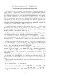
PREVIEW<br />
When the plane is viewed as the plane C <strong>of</strong> complex numbers, rotation<br />
about O through angle θ is the same as multiplication by the number<br />
e iθ = cos θ + isinθ.<br />
The set <strong>of</strong> all such numbers is the unit circle or 1-dimensional sphere<br />
S 1 = {z : |z| = 1}.<br />
Thus S 1 is not only a geometric object, but also an algebraic structure;<br />
in this case a group, under the operation <strong>of</strong> complex number multiplication.<br />
Moreover, the multiplication operation e iθ1 ·e iθ 2<br />
= e i(θ 1+θ 2 ) , and the inverse<br />
operation (e iθ ) −1 = e i(−θ ) , depend smoothly on the parameter θ. This<br />
makes S 1 an example <strong>of</strong> what we call a <strong>Lie</strong> group.<br />
However, in some respects S 1 is too special to be a good illustration <strong>of</strong><br />
<strong>Lie</strong> theory. The group S 1 is 1-dimensional and commutative, because multiplication<br />
<strong>of</strong> complex numbers is commutative. This property <strong>of</strong> complex<br />
numbers makes the <strong>Lie</strong> theory <strong>of</strong> S 1 trivial in many ways.<br />
To obtain a more interesting <strong>Lie</strong> group, we define the four-dimensional<br />
algebra <strong>of</strong> quaternions and the three-dimensional sphere S 3 <strong>of</strong> unit quaternions.<br />
Under quaternion multiplication, S 3 is a noncommutative <strong>Lie</strong> group<br />
known as SU(2), closely related to the group <strong>of</strong> space rotations.<br />
J. <strong>Stillwell</strong>, <strong>Naive</strong> <strong>Lie</strong> <strong>Theory</strong>, DOI: 10.1007/978-0-387-78214-0 1, 1<br />
c○ Springer Science+Business Media, LLC 2008
2 1 The geometry <strong>of</strong> complex numbers and quaternions<br />
1.1 Rotations <strong>of</strong> the plane<br />
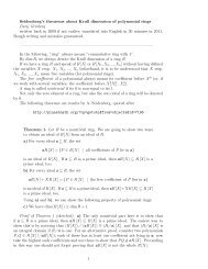
A rotation <strong>of</strong> the plane R 2 about the origin O through angle θ is a linear<br />
transformation R θ that sends the basis vectors (1,0) and (0,1) to (cos θ,<br />
sinθ) and (−sinθ,cos θ), respectively (Figure 1.1).<br />
(0,1)<br />
cosθ<br />
(cos θ,sin θ)<br />
(−sin θ,cos θ)<br />
θ<br />
θ<br />
sin θ<br />
O<br />
(1,0)<br />
Figure 1.1: Rotation <strong>of</strong> the plane through angle θ.<br />
It follows by linearity that R θ sends the general vector<br />
(x,y)=x(1,0)+y(0,1) to (xcos θ − ysinθ, xsin θ + ycosθ),<br />
and that R θ is represented by the matrix<br />
( )<br />
cosθ −sinθ<br />
.<br />
sin θ cosθ<br />
We also call this matrix R θ . Then applying the rotation to (x,y) is the same<br />
as multiplying the column vector ( x y) on the left by matrix R θ , because<br />
( ) ( )( ( )<br />
x cosθ −sinθ x xcos θ − ysinθ<br />
R θ =<br />
=<br />
.<br />
y sin θ cosθ y)<br />
xsin θ + ycosθ<br />
Since we apply matrices from the left, applying R ϕ then R θ is the same<br />
as applying the product matrix R θ R ϕ . (Admittedly, this matrix happens<br />
to equal R ϕ R θ because both equal R θ +ϕ . But when we come to space<br />
rotations the order <strong>of</strong> the matrices will be important.)
1.1 Rotations <strong>of</strong> the plane 3<br />
Thus we can represent the geometric operation <strong>of</strong> combining successive<br />
rotations by the algebraic operation <strong>of</strong> multiplying matrices. The main<br />
aim <strong>of</strong> this book is to generalize this idea, that is, to study groups <strong>of</strong> linear<br />
transformations by representing them as matrix groups. For the moment<br />
one can view a matrix group as a set <strong>of</strong> matrices that includes, along with<br />
any two members A and B, the matrices AB, A −1 ,andB −1 . Later (in Section<br />
7.2) we impose an extra condition that ensures “smoothness” <strong>of</strong> matrix<br />
groups, but the precise meaning <strong>of</strong> smoothness need not be considered yet.<br />
For those who cannot wait to see a definition, we give one in the subsection<br />
below—but be warned that its meaning will not become completely clear<br />
until Chapters 7 and 8.<br />
The matrices R θ , for all angles θ, form a group called the special orthogonal<br />
group SO(2). The reason for calling rotations “orthogonal transformations”<br />
will emerge in Chapter 3, where we generalize the idea <strong>of</strong><br />
rotation to the n-dimensional space R n and define a group SO(n) for each<br />
dimension n. In this chapter we are concerned mainly with the groups<br />
SO(2) and SO(3), which are typical in some ways, but also exceptional<br />
in having an alternative description in terms <strong>of</strong> higher-dimensional “numbers.”<br />
Each rotation R θ <strong>of</strong> R 2 can be represented by the complex number<br />
z θ = cosθ + isinθ<br />
because if we multiply an arbitrary point (x,y)=x + iy by z θ we get<br />
z θ (x + iy)=(cosθ + isinθ)(x + iy)<br />
= xcos θ − ysinθ + i(xsin θ + ycosθ)<br />
=(xcos θ − ysinθ, xsinθ + ycosθ),<br />
which is the result <strong>of</strong> rotating (x,y) through angle θ. Moreover, the ordinary<br />
product z θ z ϕ represents the result <strong>of</strong> combining R θ and R ϕ .<br />
Rotations <strong>of</strong> R 3 and R 4 can be represented, in a slightly more complicated<br />
way, by four-dimensional “numbers” called quaternions. We introduce<br />
quaternions in Section 1.3 via certain 2 × 2 complex matrices, and to<br />
pave the way for them we first investigate the relation between complex<br />
numbers and 2 × 2 real matrices in Section 1.2.<br />
What is a <strong>Lie</strong> group?<br />
The most general definition <strong>of</strong> a <strong>Lie</strong> group G is a group that is also a smooth<br />
manifold. That is, the group “product” and “inverse” operations are smooth
4 1 The geometry <strong>of</strong> complex numbers and quaternions<br />
functions on the manifold G. For readers not familiar with groups we give<br />
a crash course in Section 2.1, but we are not going to define smooth manifolds<br />
in this book, because we are not going to study general <strong>Lie</strong> groups.<br />
Instead we are going to study matrix <strong>Lie</strong> groups, which include most<br />
<strong>of</strong> the interesting <strong>Lie</strong> groups but are much easier to handle. A matrix<br />
<strong>Lie</strong> group is a set <strong>of</strong> n × n matrices (for some fixed n) that is closed under<br />
products, inverses, and nonsingular limits. The third closure condition<br />
means that if A 1 ,A 2 ,A 3 ,... is a convergent sequence <strong>of</strong> matrices in G, and<br />
A = lim k→∞ A k has an inverse, then A is in G. We say more about the limit<br />
concept for matrices in Section 4.5, but for n × n real matrices it is just the<br />
limit concept in R n2 .<br />
We can view all matrix <strong>Lie</strong> groups as groups <strong>of</strong> real matrices, but it is<br />
natural to allow the matrix entries to be complex numbers or quaternions<br />
as well. Real entries suffice in principle because complex numbers and<br />
quaternions can themselves be represented by real matrices (see Sections<br />
1.2 and 1.3).<br />
It is perhaps surprising that closure under nonsingular limits is equivalent<br />
to smoothness for matrix groups. Since we avoid the general concept<br />
<strong>of</strong> smoothness, we cannot fully explain why closed matrix groups are<br />
“smooth” in the technical sense. However, in Chapter 7 we will construct<br />
a tangent space T 1 (G) for any matrix <strong>Lie</strong> group G from tangent vectors<br />
to smooth paths in G. We find the tangent vectors using only elementary<br />
single-variable calculus, and it can also be shown that the space T 1 (G) has<br />
the same dimension as G. Thus G is “smooth” in the sense that it has a<br />
tangent space, <strong>of</strong> the appropriate dimension, at each point.<br />
Exercises<br />
Since rotation through angle θ +ϕ is the result <strong>of</strong> rotating through θ, then rotating<br />
through ϕ, we can derive formulas for sin(θ +ϕ) and cos(θ +ϕ) in terms <strong>of</strong> sinθ,<br />
sinϕ,cosθ, andcosϕ.<br />
1.1.1 Explain, by interpreting z θ+ϕ in two different ways, why<br />
Deduce that<br />
cos(θ + ϕ)+isin(θ + ϕ)=(cosθ + isinθ)(cosϕ + isinϕ).<br />
sin(θ + ϕ)=sinθ cosϕ + cosθ sinϕ,<br />
cos(θ + ϕ)=cosθ cosϕ − sinθ sinϕ.<br />
1.1.2 Deduce formulas for sin2θ and cos2θ from the formulas in Exercise 1.1.1.
1.2 Matrix representation <strong>of</strong> complex numbers 5<br />
1.1.3 Also deduce, from Exercise 1.1.1, that<br />
tan(θ + ϕ)=<br />
tanθ + tanϕ<br />
1 − tanθ tanϕ .<br />
1.1.4 Using Exercise 1.1.3, or otherwise, write down the formula for tan(θ − ϕ),<br />
and deduce that lines through O at angles θ and ϕ are perpendicular if and<br />
only if tanθ = −1/tanϕ.<br />
1.1.5 Write down the complex number z −θ and the inverse <strong>of</strong> the matrix for rotation<br />
through θ, and verify that they correspond.<br />
1.2 Matrix representation <strong>of</strong> complex numbers<br />
A good way to see why the matrices R θ = ( )<br />
cosθ −sinθ<br />
sinθ cos θ behave the same<br />
as the complex numbers z θ = cosθ + isinθ is to write R θ as the linear<br />
combination<br />
( ) ( )<br />
1 0 0 −1<br />
R θ = cosθ + sinθ<br />
0 1 1 0<br />
<strong>of</strong> the basis matrices<br />
1 =<br />
It is easily checked that<br />
( ) 1 0<br />
, i =<br />
0 1<br />
( ) 0 −1<br />
.<br />
1 0<br />
1 2 = 1, 1i = i1 = i, i 2 = −1,<br />
so the matrices 1 and i behave exactly the same as the complex numbers 1<br />
and i.<br />
In fact, the matrices<br />
( ) a −b<br />
= a1 + bi, where a,b ∈ R,<br />
b a<br />
behave exactly the same as the complex numbers a + bi under addition<br />
and multiplication, so we can represent all complex numbers by 2 × 2 real<br />
matrices, not just the complex numbers z θ that represent rotations. This<br />
representation <strong>of</strong>fers a “linear algebra explanation” <strong>of</strong> certain properties <strong>of</strong><br />
complex numbers, for example:<br />
• The squared absolute value, |a+bi| 2 = a 2 +b 2 <strong>of</strong> the complex number<br />
a + bi is the determinant <strong>of</strong> the corresponding matrix ( )<br />
a −b<br />
b a .
6 1 The geometry <strong>of</strong> complex numbers and quaternions<br />
• Therefore, the multiplicative property <strong>of</strong> absolute value, |z 1 z 2 | =<br />
|z 1 ||z 2 |, follows from the multiplicative property <strong>of</strong> determinants,<br />
det(A 1 A 2 )=det(A 1 )det(A 2 ).<br />
(Take A 1 as the matrix representing z 1 ,andA 2 as the matrix representing<br />
z 2 .)<br />
• The inverse z −1 = a−bi <strong>of</strong> z = a + bi ≠ 0 corresponds to the inverse<br />
a 2 +b 2<br />
matrix ( ) −1 a −b<br />
= 1 ( ) a b<br />
b a a 2 + b 2 .<br />
−b a<br />
The two-square identity<br />
If we set z 1 = a 1 + ib 1 and z 2 = a 2 + ib 2 , then the multiplicative property<br />
<strong>of</strong> (squared) absolute value states that<br />
(a 2 1 + b2 1 )(a2 2 + b2 2 )=(a 1a 2 − b 1 b 2 ) 2 +(a 1 b 2 + a 2 b 1 ) 2 ,<br />
as can be checked by working out the product z 1 z 2 and its squared absolute<br />
value. This identity is particularly interesting in the case <strong>of</strong> integers<br />
a 1 ,b 1 ,a 2 ,b 2 , because it says that<br />
(a sum <strong>of</strong> two squares) ×(a sum <strong>of</strong> two squares) = (a sum <strong>of</strong> two squares).<br />
This fact was noticed nearly 2000 years ago by Diophantus, who mentioned<br />
an instance <strong>of</strong> it in Book III, Problem 19, <strong>of</strong> his Arithmetica. However,<br />
Diophantus said nothing about sums <strong>of</strong> three squares—with good reason,<br />
because there is no such three-square identity. For example<br />
(1 2 + 1 2 + 1 2 )(0 2 + 1 2 + 2 2 )=3 × 5 = 15,<br />
and15isnot a sum <strong>of</strong> three integer squares.<br />
This is an early warning sign that there are no three-dimensional numbers.<br />
In fact, there are no n-dimensional numbers for any n > 2; however,<br />
there is a “near miss” for n = 4. One can define “addition” and “multiplication”<br />
for quadruples q =(a,b,c,d) <strong>of</strong> real numbers so as to satisfy all<br />
the basic laws <strong>of</strong> arithmetic except q 1 q 2 = q 2 q 1 (the commutative law <strong>of</strong><br />
multiplication). This system <strong>of</strong> arithmetic for quadruples is the quaternion<br />
algebra that we introduce in the next section.
1.3 Quaternions 7<br />
Exercises<br />
1.2.1 Derive the two-square identity from the multiplicative property <strong>of</strong> det.<br />
1.2.2 Write 5 and 13 as sums <strong>of</strong> two squares, and hence express 65 as a sum <strong>of</strong><br />
two squares using the two-square identity.<br />
1.2.3 Using the two-square identity, express 37 2 and 37 4 as sums <strong>of</strong> two nonzero<br />
squares.<br />
The absolute value |z| = √ a 2 + b 2 represents the distance <strong>of</strong> z from O, and<br />
more generally, |u − v| represents the distance between u and v. When combined<br />
with the distributive law,<br />
u(v − w)=uv − uw,<br />
a geometric property <strong>of</strong> multiplication comes to light.<br />
1.2.4 Deduce, from the distributive law and multiplicative absolute value, that<br />
|uv − uw| = |u||v − w|.<br />
Explain why this says that multiplication <strong>of</strong> the whole plane <strong>of</strong> complex<br />
numbers by u multiplies all distances by |u|.<br />
1.2.5 Deduce from Exercise 1.2.4 that multiplication <strong>of</strong> the whole plane <strong>of</strong> complex<br />
numbers by cosθ + isinθ leaves all distances unchanged.<br />
A map that leaves all distances unchanged is called an isometry (from the<br />
Greek for “same measure”), so multiplication by cosθ + isinθ is an isometry <strong>of</strong><br />
the plane. (In Section 1.1 we defined the corresponding rotation map R θ as a linear<br />
map that moves 1 and i in a certain way; it is not obvious from this definition that<br />
a rotation is an isometry.)<br />
1.3 Quaternions<br />
By associating the ordered pair (a,b) with the complex number a+ib or the<br />
matrix ( )<br />
a −b<br />
b a we can speak <strong>of</strong> the “sum,” “product,” and “absolute value”<br />
<strong>of</strong> ordered pairs. In the same way, we can speak <strong>of</strong> the “sum,” “product,”<br />
and “absolute value” <strong>of</strong> ordered quadruples by associating each ordered<br />
quadruple (a,b,c,d) <strong>of</strong> real numbers with the matrix<br />
( )<br />
a + id −b − ic<br />
q =<br />
. (*)<br />
b − ic a − id<br />
We call any matrix <strong>of</strong> the form (*) a quaternion. (This is not the only<br />
way to associate a matrix with a quadruple. I have chosen these complex
8 1 The geometry <strong>of</strong> complex numbers and quaternions<br />
matrices because they extend the real matrices used in the previous section<br />
to represent complex numbers. Thus complex numbers are the special<br />
quaternions with c = d = 0.)<br />
It is clear that the sum <strong>of</strong> any two matrices <strong>of</strong> the form (*) is another<br />
matrix <strong>of</strong> the same form, and it can be checked (Exercise 1.3.2) that the<br />
product <strong>of</strong> two matrices <strong>of</strong> the form (*) is <strong>of</strong> the form (*). Thus we can<br />
define the sum and product <strong>of</strong> quaternions to be just the matrix sum and<br />
product. Also, if the squared absolute value |q| 2 <strong>of</strong> a quaternion q is defined<br />
to be the determinant <strong>of</strong> q, thenwehave<br />
( )<br />
a + id −b − ic<br />
det q = det<br />
= a 2 + b 2 + c 2 + d 2 .<br />
b − ic a − id<br />
So |q| 2 is the squared distance <strong>of</strong> the point (a,b,c,d) from O in R 4 .<br />
The quaternion sum operation has the same basic properties as addition<br />
for numbers, namely<br />
q 1 + q 2 = q 2 + q 1 ,<br />
(commutative law)<br />
q 1 +(q 2 + q 3 )=(q 1 + q 2 )+q 3 ,<br />
(associative law)<br />
q +(−q)=0 where 0 is the zero matrix, (inverse law)<br />
q + 0 = q.<br />
(identity law)<br />
The quaternion product operation does not have all the properties <strong>of</strong><br />
multiplication <strong>of</strong> numbers—in general, the commutative property q 1 q 2 =<br />
q 2 q 1 fails—but well-known properties <strong>of</strong> the matrix product imply the following<br />
properties <strong>of</strong> the quaternion product:<br />
q 1 (q 2 q 3 )=(q 1 q 2 )q 3 ,<br />
(associative law)<br />
qq −1 = 1 for q ≠ 0, (inverse law)<br />
q1 = q,<br />
(identity law)<br />
q 1 (q 2 + q 3 )=q 1 q 2 + q 1 q 3 .<br />
(left distributive law)<br />
Here 0 and 1 denote the 2 × 2 zero and identity matrices, which are also<br />
quaternions. The right distributive law (q 2 +q 3 )q 1 = q 2 q 1 +q 3 q 1 <strong>of</strong> course<br />
holds too, and is distinct from the left distributive law because <strong>of</strong> the noncommutative<br />
product.<br />
The noncommutative nature <strong>of</strong> the quaternion product is exposed more<br />
clearly when we write<br />
( )<br />
a + di −b − ci<br />
= a1 + bi + cj + dk,<br />
b − ci a − di
1.3 Quaternions 9<br />
where<br />
1 =<br />
( ) 1 0<br />
, i =<br />
0 1<br />
( ) 0 −1<br />
, j =<br />
1 0<br />
( ) ( )<br />
0 −i i 0<br />
, k = .<br />
−i 0<br />
0 −i<br />
Thus 1 behaves like the number 1, i 2 = −1 as before, and also j 2 = k 2 =<br />
−1. The noncommutativity is concentrated in the products <strong>of</strong> i, j, k,which<br />
are summarized in Figure 1.2. The product <strong>of</strong> any two distinct elements is<br />
i<br />
k<br />
j<br />
Figure 1.2: Products <strong>of</strong> the imaginary quaternion units.<br />
the third element in the circle, with a + sign if an arrow points from the<br />
first element to the second, and a − sign otherwise. For example, ij = k,<br />
but ji = −k,soij ≠ ji.<br />
The failure <strong>of</strong> the commutative law is actually a good thing, because it<br />
enables quaternions to represent other things that do not commute, such as<br />
rotations in three and four dimensions.<br />
As with complex numbers, there is a linear algebra explanation <strong>of</strong> some<br />
less obvious properties <strong>of</strong> quaternion multiplication.<br />
• The absolute value has the multiplicative property |q 1 q 2 | = |q 1 ||q 2 |,<br />
by the multiplicative property <strong>of</strong> det: det(q 1 q 2 )=det(q 1 )det(q 2 ).<br />
• Each nonzero quaternion q has an inverse q −1 , namely the matrix<br />
inverse <strong>of</strong> q.<br />
• From the matrix (*) for q we get an explicit formula for q −1 . If<br />
q = a1 + bi + cj + dk ≠ 0then<br />
q −1 =<br />
1<br />
a 2 + b 2 + c 2 (a1 − bi − cj − dk).<br />
+ d2 • The quaternion a1 − bi − cj − dk is called the quaternion conjugate<br />
q <strong>of</strong> q = a1+bi+cj+dk, and we have qq = a 2 +b 2 +c 2 +d 2 = |q| 2 .
10 1 The geometry <strong>of</strong> complex numbers and quaternions<br />
• The quaternion conjugate is not the result <strong>of</strong> taking the complex conjugate<br />
<strong>of</strong> each entry in the matrix q. In fact, q is the result <strong>of</strong> taking<br />
the complex conjugate <strong>of</strong> each entry in the transposed matrix q T .<br />
Then it follows from (q 1 q 2 ) T = q T 2 qT 1 that (q 1q 2 )=q 2 q 1 .<br />
The algebra <strong>of</strong> quaternions was discovered by Hamilton in 1843, and<br />
it is denoted by H in his honor. He started with just i and j (hoping to<br />
find an algebra <strong>of</strong> triples analogous to the complex algebra <strong>of</strong> pairs), but<br />
later introduced k = ij to escape from apparently intractable problems with<br />
triples (he did not know, at first, that there is no three-square identity). The<br />
matrix representation was discovered in 1858, by Cayley.<br />
The 3-sphere <strong>of</strong> unit quaternions<br />
The quaternions a1 + bi + cj + dk <strong>of</strong> absolute value 1, or unit quaternions,<br />
satisfy the equation<br />
a 2 + b 2 + c 2 + d 2 = 1.<br />
Hence they form the analogue <strong>of</strong> the sphere, called the 3-sphere S 3 ,inthe<br />
space R 4 <strong>of</strong> all 4-tuples (a,b,c,d). It follows from the multiplicative property<br />
and the formula for inverses above that the product <strong>of</strong> unit quaternions<br />
is again a unit quaternion, and hence S 3 is a group under quaternion multiplication.<br />
Like the 1-sphere S 1 <strong>of</strong> unit complex numbers, the 3-sphere<br />
<strong>of</strong> unit quaternions encapsulates a group <strong>of</strong> rotations, though not quite so<br />
directly. In the next two sections we show how unit quaternions may be<br />
used to represent rotations <strong>of</strong> ordinary space R 3 .<br />
Exercises<br />
When Hamilton discovered H he described quaternion multiplication very concisely<br />
by the relations<br />
i 2 = j 2 = k 2 = ijk = −1.<br />
1.3.1 Verify that Hamilton’s relations hold for the matrices 1, i, j, andk. Also<br />
show (assuming associativity and inverses) that these relations imply all<br />
the products <strong>of</strong> i, j,andk showninFigure1.2.<br />
1.3.2 Verify that the product <strong>of</strong> quaternions is indeed a quaternion. (Hint: It helps<br />
to write each quaternion in the form<br />
( ) α −β<br />
q = ,<br />
β α<br />
where α = x − iy is the complex conjugate <strong>of</strong> α = x + iy.)
1.4 Consequences <strong>of</strong> multiplicative absolute value 11<br />
1.3.3 Check that q is the result <strong>of</strong> taking the complex conjugate <strong>of</strong> each entry in<br />
q T , and hence show that q 1 q 2 = q 2 q 1 for any quaternions q 1 and q 2 .<br />
1.3.4 Also check that qq = |q| 2 .<br />
Cayley’s matrix representation makes it easy (in principle) to derive an amazing<br />
algebraic identity.<br />
1.3.5 Show that the multiplicative property <strong>of</strong> determinants gives the complex<br />
two-square identity (discovered by Gauss around 1820)<br />
(|α 1 | 2 + |β 1 | 2 )(|α 2 | 2 + |β 2 | 2 )=|α 1 α 2 − β 1 β 2 | 2 + |α 1 β 2 + β 1 α 2 | 2 .<br />
1.3.6 Show that the multiplicative property <strong>of</strong> determinants gives the real foursquare<br />
identity<br />
(a 2 1 + b2 1 + c2 1 + d2 1 )(a2 2 + b2 2 + c2 2 + d2 2 )= (a 1a 2 − b 1 b 2 − c 1 c 2 − d 1 d 2 ) 2<br />
+(a 1 b 2 + b 1 a 2 + c 1 d 2 − d 1 c 2 ) 2<br />
+(a 1 c 2 − b 1 d 2 + c 1 a 2 + d 1 b 2 ) 2<br />
+(a 1 d 2 + b 1 c 2 − c 1 b 2 + d 1 a 2 ) 2 .<br />
This identity was discovered by Euler in 1748, nearly 100 years before the discovery<br />
<strong>of</strong> quaternions! Like Diophantus, he was interested in the case <strong>of</strong> integer<br />
squares, in which case the identity says that<br />
(a sum <strong>of</strong> four squares)× (a sum <strong>of</strong> four squares) = (a sum <strong>of</strong> four squares).<br />
This was the first step toward proving the theorem that every positive integer is<br />
the sum <strong>of</strong> four integer squares. The pro<strong>of</strong> was completed by Lagrange in 1770.<br />
1.3.7 Express 97 and 99 as sums <strong>of</strong> four squares.<br />
1.3.8 Using Exercise 1.3.6, or otherwise, express 97×99 as a sum <strong>of</strong> four squares.<br />
1.4 Consequences <strong>of</strong> multiplicative absolute value<br />
The multiplicative absolute value, for both complex numbers and quaternions,<br />
first appeared in number theory as a property <strong>of</strong> sums <strong>of</strong> squares. It<br />
was noticed only later that it has geometric implications, relating multiplication<br />
to rigid motions <strong>of</strong> R 2 , R 3 ,andR 4 . Suppose first that u is a complex<br />
number <strong>of</strong> absolute value 1. Without any computation with cosθ and sinθ,<br />
we can see that multiplication <strong>of</strong> C = R 2 by u is a rotation <strong>of</strong> the plane as<br />
follows.
12 1 The geometry <strong>of</strong> complex numbers and quaternions<br />
Let v and w be any two complex numbers, and consider their images,<br />
uv and uw under multiplication by u. Thenwehave<br />
distance from uv to uw = |uv − uw|<br />
= |u(v − w)| by the distributive law<br />
= |u||v − w| by multiplicative absolute value<br />
= |v − w| because |u| = 1<br />
= distance from v to w.<br />
In other words, multiplication by u with |u| = 1 is a rigid motion, also<br />
known as an isometry, <strong>of</strong> the plane. Moreover, this isometry leaves O<br />
fixed, because u × 0 = 0. And if u ≠ 1, no other point v is fixed, because<br />
uv = v implies u = 1. The only motion <strong>of</strong> the plane with these properties<br />
is rotation about O.<br />
Exactly the same argument applies to quaternion multiplication, at least<br />
as far as preservation <strong>of</strong> distance is concerned: if we multiply the space<br />
R 4 <strong>of</strong> quaternions by a quaternion <strong>of</strong> absolute value 1, then the result is<br />
an isometry <strong>of</strong> R 4 that leaves the origin fixed. It is in fact reasonable to<br />
interpret this isometry <strong>of</strong> R 4 as a “rotation,” but first we want to show that<br />
quaternion multiplication also gives a way to study rotations <strong>of</strong> R 3 . To see<br />
how, we look at a natural three-dimensional subspace <strong>of</strong> the quaternions.<br />
Pure imaginary quaternions<br />
The pure imaginary quaternions are those <strong>of</strong> the form<br />
p = bi + cj + dk.<br />
They form a three-dimensional space that we will denote by Ri+Rj+Rk,<br />
or sometimes R 3 for short. The space Ri + Rj + Rk is the orthogonal<br />
complement to the line R1 <strong>of</strong> quaternions <strong>of</strong> the form a1, which we will<br />
call real quaternions. From now on we write the real quaternion a1 simply<br />
as a, and denote the line <strong>of</strong> real quaternions simply by R.<br />
It is clear that the sum <strong>of</strong> any two members <strong>of</strong> Ri + Rj + Rk is itself<br />
amember<strong>of</strong>Ri + Rj + Rk, but this is not generally true <strong>of</strong> products. In<br />
fact, if u = u 1 i + u 2 j + u 3 k and v = v 1 i + v 2 j + v 3 k then the multiplication<br />
diagram for i, j, andk (Figure 1.2) gives<br />
uv = − (u 1 v 1 + u 2 v 2 + u 3 v 3 )<br />
+(u 2 v 3 − u 3 v 2 )i − (u 1 v 3 − u 3 v 1 )j +(u 1 v 2 − u 2 v 1 )k.
1.4 Consequences <strong>of</strong> multiplicative absolute value 13<br />
This relates the quaternion product uv to two other products on R 3 that are<br />
well known in linear algebra: the inner (or “scalar” or “dot”) product,<br />
u · v = u 1 v 1 + u 2 v 2 + u 3 v 3 ,<br />
and the vector (or “cross”) product<br />
∣ i j k ∣∣∣∣∣<br />
u × v =<br />
u 1 u 2 u 3 =(u 2 v 3 − u 3 v 2 )i − (u 1 v 3 − u 3 v 1 )j +(u 1 v 2 − u 2 v 1 )k.<br />
∣v 1 v 2 v 3<br />
In terms <strong>of</strong> the scalar and vector products, the quaternion product is<br />
uv = −u · v + u × v.<br />
Since u · v is a real number, this formula shows that uv is in Ri + Rj + Rk<br />
only if u · v = 0, that is, only if u is orthogonal to v.<br />
The formula uv = −u · v + u × v also shows that uv is real if and only<br />
if u × v = 0, that is, if u and v have the same (or opposite) direction. In<br />
particular, if u ∈ Ri + Rj + Rk and |u| = 1 then<br />
u 2 = −u · u = −|u| 2 = −1.<br />
Thus every unit vector in Ri + Rj + Rk is a “square root <strong>of</strong> −1.” (This, by<br />
the way, is another sign that H does not satisfy all the usual laws <strong>of</strong> algebra.<br />
If it did, the equation u 2 = −1 would have at most two solutions.)<br />
Exercises<br />
The cross product is an operation on Ri+Rj+Rk because u×v is in Ri+Rj+Rk<br />
for any u,v ∈ Ri + Rj + Rk. However, it is neither a commutative nor associative<br />
operation, as Exercises 1.4.1 and 1.4.3 show.<br />
1.4.1 Prove the antisymmetric property u × v = −v × u.<br />
1.4.2 Prove that u × (v × w)=v(u · w) − w(u · v) for pure imaginary u,v,w.<br />
1.4.3 Deduce from Exercise 1.4.2 that × is not associative.<br />
1.4.4 Also deduce the Jacobi identity for the cross product:<br />
u × (v × w)+w × (u × v)+v × (w × u)=0.<br />
The antisymmetric and Jacobi properties show that the cross product is not completely<br />
lawless. These properties define what we later call a <strong>Lie</strong> algebra.
14 1 The geometry <strong>of</strong> complex numbers and quaternions<br />
1.5 Quaternion representation <strong>of</strong> space rotations<br />
A quaternion t <strong>of</strong> absolute value 1, like a complex number <strong>of</strong> absolute value<br />
1, has a “real part” cos θ and an “imaginary part” <strong>of</strong> absolute value sinθ,<br />
orthogonal to the real part and hence in Ri + Rj + Rk. This means that<br />
t = cosθ + usinθ,<br />
where u is a unit vector in Ri+Rj+Rk, and hence u 2 = −1 by the remark<br />
at the end <strong>of</strong> the previous section.<br />
Such a unit quaternion t induces a rotation <strong>of</strong> Ri + Rj + Rk, though<br />
not simply by multiplication, since the product <strong>of</strong> t and a member q <strong>of</strong><br />
Ri + Rj + Rk may not belong to Ri + Rj + Rk. Instead, we send each<br />
q ∈ Ri+Rj+Rk to t −1 qt, which turns out to be a member <strong>of</strong> Ri+Rj+Rk.<br />
To see why, first note that<br />
t −1 = t/|t| 2 = cosθ − usinθ,<br />
by the formulas for q −1 and q in Section 1.3.<br />
Since t −1 exists, multiplication <strong>of</strong> H on either side by t or t −1 is an<br />
invertible map and hence a bijection <strong>of</strong> H onto itself. It follows that the<br />
map q ↦→ t −1 qt, called conjugation by t, is a bijection <strong>of</strong> H. Conjugation by<br />
t also maps the real line R onto itself, because t −1 rt = r for a real number<br />
r; hence it also maps the orthogonal complement Ri + Rj + Rk onto itself.<br />
This is because conjugation by t is an isometry, since multiplication on<br />
either side by a unit quaternion is an isometry.<br />
It looks as though we are onto something with conjugation by t =<br />
cosθ + usinθ, and indeed we have the following theorem.<br />
Rotation by conjugation. If t = cosθ + usinθ, whereu∈ Ri + Rj + Rk<br />
is a unit vector, then conjugation by t rotates Ri + Rj + Rk through angle<br />
2θ about axis u.<br />
Pro<strong>of</strong>. First, observe that the line Ru <strong>of</strong> real multiples <strong>of</strong> u is fixed by the<br />
conjugation map, because<br />
t −1 ut =(cos θ − usinθ)u(cos θ + usinθ)<br />
=(ucos θ − u 2 sinθ)(cos θ + usinθ)<br />
=(ucos θ + sinθ)(cos θ + usinθ) because u 2 = −1<br />
= u(cos 2 θ + sin 2 θ)+sinθ cosθ + u 2 sinθ cosθ<br />
= u also because u 2 = −1.
1.5 Quaternion representation <strong>of</strong> space rotations 15<br />
It follows, since conjugation by t is an isometry <strong>of</strong> Ri + Rj + Rk, that<br />
its restriction to the plane through O in Ri+Rj+Rk orthogonal to the line<br />
Ru is also an isometry. And if the restriction to this plane is a rotation, then<br />
conjugation by t is a rotation <strong>of</strong> the whole space Ri + Rj + Rk.<br />
To see whether this is indeed the case, choose a unit vector v orthogonal<br />
to u in Ri + Rj + Rk, sou · v = 0. Then let w = u × v, which equals uv<br />
because u·v = 0, so {u,v,w} is an orthonormal basis <strong>of</strong> Ri+Rj+Rk with<br />
uv = w, vw = u, wu = v, uv = −vu and so on. It remains to show that<br />
t −1 vt = vcos 2θ − wsin2θ,<br />
t −1 wt = vsin 2θ + wcos2θ,<br />
because this means that conjugation by t rotates the basis vectors v and w,<br />
and hence the whole plane orthogonal to the line Ru, through angle 2θ.<br />
This is confirmed by the following computation:<br />
t −1 vt =(cos θ − usinθ)v(cos θ + usinθ)<br />
=(vcos θ − uvsinθ)(cos θ + usinθ)<br />
= vcos 2 θ − uvsinθ cosθ + vusinθ cosθ − uvusin 2 θ<br />
= vcos 2 θ − 2uvsin θ cos θ + u 2 vsin 2 θ because vu = −uv<br />
= v(cos 2 θ − sin 2 θ) − 2wsinθ cosθ because u 2 = −1, uv = w<br />
= vcos 2θ − wsin2θ.<br />
A similar computation (try it) shows that t −1 wt = vsin 2θ + wcos2θ, as<br />
required.<br />
□<br />
This theorem shows that every rotation <strong>of</strong> R 3 , given by an axis u and<br />
angle <strong>of</strong> rotation α, is the result <strong>of</strong> conjugation by the unit quaternion<br />
t = cos α 2 + usin α 2 .<br />
The same rotation is induced by −t, since(−t) −1 s(−t) =t −1 st. But ±t<br />
are the only unit quaternions that induce this rotation, because each unit<br />
quaternion is uniquely expressible in the form t = cos α 2 + usin α 2 ,andthe<br />
rotation is uniquely determined by the two (axis, angle) pairs (u,α) and<br />
(−u,−α). The quaternions t and −t are said to be antipodal, because they<br />
represent diametrically opposite points on the 3-sphere <strong>of</strong> unit quaternions.<br />
Thus the theorem says that rotations <strong>of</strong> R 3 correspond to antipodal<br />
pairs <strong>of</strong> unit quaternions. We also have the following important corollary.
16 1 The geometry <strong>of</strong> complex numbers and quaternions<br />
Rotations form a group. The product <strong>of</strong> rotations is a rotation, and the<br />
inverse <strong>of</strong> a rotation is a rotation.<br />
Pro<strong>of</strong>. The inverse <strong>of</strong> the rotation about axis u through angle α is obviously<br />
a rotation, namely, the rotation about axis u through angle −α.<br />
It is not obvious what the product <strong>of</strong> two rotations is, but we can show<br />
as follows that it has an axis and angle <strong>of</strong> rotation, and hence is a rotation.<br />
Suppose we are given a rotation r 1 with axis u 1 and angle α 1 , and a rotation<br />
r 2 with axis u 2 and angle α 2 .Then<br />
r 1 is induced by conjugation by t 1 = cos α 1<br />
2 + u 1 sin α 1<br />
2<br />
and<br />
r 2 is induced by conjugation by t 2 = cos α 2<br />
2 + u 2 sin α 2<br />
2 ,<br />
hence the result r 1 r 2 <strong>of</strong> doing r 1 ,thenr 2 , is induced by<br />
q ↦→ t −1<br />
2 (t−1 1 qt 1)t 2 =(t 1 t 2 ) −1 q(t 1 t 2 ),<br />
which is conjugation by t 1 t 2 = t. The quaternion t is also a unit quaternion,<br />
so<br />
t = cos α 2 + usin α 2<br />
for some unit imaginary quaternion u and angle α. Thus the product rotation<br />
is the rotation about axis u through angle α.<br />
□<br />
The pro<strong>of</strong> shows that the axis and angle <strong>of</strong> the product rotation r 1 r 2 can<br />
in principle be found from those <strong>of</strong> r 1 and r 2 by quaternion multiplication.<br />
They may also be described geometrically, by the alternative pro<strong>of</strong> <strong>of</strong> the<br />
group property given in the exercises below.<br />
Exercises<br />
The following exercises introduce a small fragment <strong>of</strong> the geometry <strong>of</strong> isometries:<br />
that any rotation <strong>of</strong> the plane or space is a product <strong>of</strong> two reflections. We begin<br />
with the simplest case: representing rotation <strong>of</strong> the plane about O through angle<br />
θ as the product <strong>of</strong> reflections in two lines through O.<br />
If L is any line in the plane, then reflection in L is the transformation <strong>of</strong> the<br />
plane that sends each point S to the point S ′ such that SS ′ is orthogonal to L and<br />
L is equidistant from S and S ′ .
1.5 Quaternion representation <strong>of</strong> space rotations 17<br />
S ′<br />
P<br />
α<br />
α<br />
S<br />
L<br />
Figure 1.3: Reflection <strong>of</strong> S and its angle.<br />
1.5.1 If L passes through P,andifS lies on one side <strong>of</strong> L at angle α (Figure 1.3),<br />
show that S ′ lies on the other side <strong>of</strong> L at angle α,andthat|PS| = |PS ′ |.<br />
1.5.2 Deduce, from Exercise 1.5.1 or otherwise, that the rotation about P through<br />
angle θ is the result <strong>of</strong> reflections in any two lines through P that meet at<br />
angle θ/2.<br />
1.5.3 Deduce, from Exercise 1.5.2 or otherwise, that if L , M ,andN are lines<br />
situated as shown in Figure 1.4, then the result <strong>of</strong> rotation about P through<br />
angle θ, followed by rotation about Q through angle ϕ, is rotation about R<br />
through angle χ (with rotations in the senses indicated by the arrows).<br />
P<br />
R<br />
χ/2<br />
L<br />
N<br />
θ/2<br />
ϕ/2<br />
M<br />
Q<br />
Figure 1.4: Three lines and three rotations.<br />
1.5.4 If L and N are parallel, so R does not exist, what isometry is the result <strong>of</strong><br />
the rotations about P and Q?<br />
Now we extend these ideas to R 3 .Arotation about a line through O (called<br />
the axis <strong>of</strong> rotation) is the product <strong>of</strong> reflections in planes through O that meet<br />
along the axis. To make the reflections easier to visualize, we do not draw the<br />
planes, but only their intersections with the unit sphere (see Figure 1.5).<br />
These intersections are curves called great circles, andreflection in a great<br />
circle is the restriction to the sphere <strong>of</strong> reflection in a plane through O.
18 1 The geometry <strong>of</strong> complex numbers and quaternions<br />
R<br />
L<br />
θ/2<br />
P<br />
N<br />
ϕ/2<br />
M<br />
Q<br />
Figure 1.5: Reflections in great circles on the sphere.<br />
1.5.5 Adapt the argument <strong>of</strong> Exercise 1.5.3 to great circles L , M ,andN shown<br />
in Figure 1.5. What is the conclusion?<br />
1.5.6 Explain why there is no exceptional case analogous to Exercise 1.5.4. Deduce<br />
that the product <strong>of</strong> any two rotations <strong>of</strong> R 3 about O is another rotation<br />
about O, and explain how to find the axis <strong>of</strong> the product rotation.<br />
The idea <strong>of</strong> representing isometries as products <strong>of</strong> reflections is also useful in<br />
higher dimensions. We use this idea again in Section 2.4, where we show that any<br />
isometry <strong>of</strong> R n that fixes O is the product <strong>of</strong> at most n reflections in hyperplanes<br />
through O.<br />
1.6 Discussion<br />
The geometric properties <strong>of</strong> complex numbers were discovered long before<br />
the complex numbers themselves. Diophantus (already mentioned in Section<br />
1.2) was aware <strong>of</strong> the two-square identity, and indeed he associated a<br />
sum <strong>of</strong> two squares, a 2 +b 2 , with the right-angled triangle with perpendicular<br />
sides a and b. Thus, Diophantus was vaguely aware <strong>of</strong> two-dimensional<br />
objects (right-angled triangles) with a multiplicative property (<strong>of</strong> their hypotenuses).<br />
Around 1590, Viète noticed that the Diophantus “product”<br />
<strong>of</strong> triangles with sides (a,b) and (c,d)—namely, the triangle with sides<br />
(ac − bd,bc + ad)—also has an additive property, <strong>of</strong> angles (Figure 1.6).
1.6 Discussion 19<br />
√<br />
a 2 + b 2<br />
θ<br />
a<br />
b<br />
×<br />
√<br />
c 2 + d 2<br />
ϕ<br />
c<br />
d<br />
=<br />
√<br />
(a 2 + b 2 )(c 2 + d 2 )<br />
θ + ϕ<br />
ac − bd<br />
bc + ad<br />
Figure 1.6: The Diophantus “product” <strong>of</strong> triangles.<br />
The algebra <strong>of</strong> complex numbers emerged from the study <strong>of</strong> polynomial<br />
equations in the sixteenth century, particularly the solution <strong>of</strong> cubic<br />
equations by the Italian mathematicians del Ferro, Tartaglia, Cardano,<br />
and Bombelli. Complex numbers were not required for the solution <strong>of</strong><br />
quadratic equations, because in the sixteenth century one could say that<br />
x 2 + 1 = 0, for example, has no solution. The formal solution x = √ −1<br />
was just a signal that no solution really exists. Cubic equations force the<br />
issue because the equation x 3 = px + q has solution<br />
√<br />
√<br />
√<br />
x = 3 q (q 2 ( p<br />
)<br />
√<br />
3<br />
2 2) + 3 q (q 2 ( p<br />
) 3<br />
− +<br />
3 2 2) − −<br />
3<br />
(the “Cardano formula”). Thus, according to the Cardano formula the solution<br />
<strong>of</strong> x 3 = 15x + 4is<br />
√<br />
√ √<br />
x =<br />
√2 3 + 2 2 − 5 3 +<br />
√2 3 − 2 2 − 5 3 = 3 2 + 11i +<br />
3√<br />
2 − 11i.<br />
But the symbol i = √ −1 cannot be signaling NO SOLUTION here, because<br />
there is an obvious solution x = 4. How can 3 √<br />
2 + 11i +<br />
3√<br />
2 − 11i be the<br />
solution when 4 is?<br />
In 1572, Bombelli resolved this conflict, and launched the algebra <strong>of</strong><br />
complex numbers, by observing that<br />
(2 + i) 3 = 2 + 11i, (2 − i) 3 = 2 − 11i,
20 1 The geometry <strong>of</strong> complex numbers and quaternions<br />
and therefore<br />
3√<br />
2 + 11i +<br />
3√<br />
2 − 11i =(2 + i)+(2 − i)=4,<br />
assuming that i obeys the same rules as ordinary, real, numbers. His calculation<br />
was, in effect, an experimental test <strong>of</strong> the proposition that complex<br />
numbers form a field—a proposition that could not have been formulated,<br />
let alone proved, at the time. The first rigorous treatment <strong>of</strong> complex numbers<br />
was that <strong>of</strong> Hamilton, who in 1835 gave definitions <strong>of</strong> complex numbers,<br />
addition, and multiplication that make a pro<strong>of</strong> <strong>of</strong> the field properties<br />
crystal clear.<br />
Hamilton defined complex numbers as ordered pairs z =(a,b) <strong>of</strong> real<br />
numbers, and he defined their sum and product by<br />
(a 1 ,b 1 )+(a 2 ,b 2 )=(a 1 + a 2 ,b 1 + b 2 ),<br />
(a 1 ,b 1 )(a 2 ,b 2 )=(a 1 a 2 − b 1 b 2 ,a 1 b 2 + b 1 a 2 ).<br />
Of course, these definitions are motivated by the interpretation <strong>of</strong> (a,b) as<br />
a + ib, wherei 2 = −1, but the important point is that the field properties<br />
follow from these definitions and the properties <strong>of</strong> real numbers. The properties<br />
<strong>of</strong> addition are directly “inherited” from properties <strong>of</strong> real number<br />
addition. For example, for complex numbers z 1 =(a 1 ,b 1 ) and z 2 =(a 2 ,b 2 )<br />
we have<br />
z 1 + z 2 = z 2 + z 1<br />
because<br />
a 1 + a 2 = a 2 + a 1 and b 1 + b 2 = b 2 + b 1 for real numbers a 1 ,a 2 ,b 1 ,b 2 .<br />
Indeed, the properties <strong>of</strong> addition are not special properties <strong>of</strong> pairs, they<br />
also hold for the vector sum <strong>of</strong> triples, quadruples, and so on. The field<br />
properties <strong>of</strong> multiplication, on the other hand, depend on the curious definition<br />
<strong>of</strong> product <strong>of</strong> pairs, which has no obvious generalization to a product<br />
<strong>of</strong> n-tuples for n > 2.<br />
This raises the question; is it possible to define a “product” operation on<br />
R n that, together with the vector sum operation, makes R n a field? Hamilton<br />
hoped to find such a product for each n. Indeed, he hoped to find a<br />
product with not only the field properties but also the multiplicative absolute<br />
value<br />
|uv| = |u||v|,
1.6 Discussion 21<br />
√<br />
where the absolute value <strong>of</strong> u =(x 1 ,x 2 ,...,x n ) is |u| = x 2 1 + x2 2 + ···+ x2 n.<br />
As we have seen, for n = 2 this property is equivalent to the Diophantus<br />
identity for sums <strong>of</strong> two squares, so a multiplicative absolute value in general<br />
implies an identity for sums <strong>of</strong> n squares.<br />
Hamilton attacked the problem from the opposite direction, as it were.<br />
He tried to define the product operation, first for triples, before worrying<br />
about the absolute value. But after searching fruitlessly for 13 years, he<br />
had to admit defeat. He still had not noticed that there is no three square<br />
identity, but he suspected that multiplying triples <strong>of</strong> the form a + bi + cj<br />
requires a new object k = ij. Also, he began to realize that there is no hope<br />
for the commutative law <strong>of</strong> multiplication. Desperate to salvage something<br />
from his 13 years <strong>of</strong> work, he made the leap to the fourth dimension. He<br />
took k = ij to be a vector perpendicular to 1, i, and j, and sacrificed the<br />
commutative law by allowing ij= − ji, jk = −kj,andki = −ik. OnOctober<br />
16, 1843 he had his famous epiphany that i, j, andk must satisfy<br />
i 2 = j 2 = k 2 = ijk= −1.<br />
As we have seen in Section 1.3, these relations imply all the field properties,<br />
except commutative multiplication. Such a system is <strong>of</strong>ten called<br />
a skew field (though this term unfortunately suggests a specialization <strong>of</strong><br />
the field concept, rather than what it really is—a generalization). Hamilton’s<br />
relations also imply that absolute value is multiplicative—a fact he<br />
had to check, though the equivalent four-square identity was well known<br />
to number theorists.<br />
In 1878, Frobenius proved that the quaternion algebra H is the only<br />
skew field R n that is not a field, so Hamilton had found the only “algebra<br />
<strong>of</strong> n-tuples” it was possible to find under the conditions he had imposed.<br />
The multiplicative absolute value, as stressed in Section 1.4, implies<br />
that multiplication by a quaternion <strong>of</strong> absolute value 1 is an isometry <strong>of</strong><br />
R 4 . Hamilton seems to have overlooked this important geometric fact, and<br />
the quaternion representation <strong>of</strong> space rotations (Section 1.5) was first published<br />
by Cayley in 1845. Cayley also noticed that the corresponding formulas<br />
for transforming the coordinates <strong>of</strong> R 3 had been given by Rodrigues<br />
in 1840. Cayley’s discovery showed that the noncommutative quaternion<br />
product is a good thing, because space rotations are certainly noncommutative;<br />
hence they can be faithfully represented only by a noncommutative<br />
algebra. This finding has been enthusiastically endorsed by the computer<br />
graphics pr<strong>of</strong>ession today, which uses quaternions as a standard tool for
22 1 The geometry <strong>of</strong> complex numbers and quaternions<br />
rendering 3-dimensional motion.<br />
The quaternion algebra H plays two roles in <strong>Lie</strong> theory. On the one<br />
hand, H gives the most understandable treatment <strong>of</strong> rotations in R 3 and R 4 ,<br />
and hence <strong>of</strong> the rotation groups <strong>of</strong> these two spaces. The rotation groups<br />
<strong>of</strong> R 3 and R 4 are <strong>Lie</strong> groups, and they illustrate many general features <strong>of</strong><br />
<strong>Lie</strong> theory in a way that is easy to visualize and compute. On the other<br />
hand, H also provides coordinates for an infinite series <strong>of</strong> spaces H n , with<br />
properties closely analogous to those <strong>of</strong> the spaces R n and C n . In particular,<br />
we can generalize the concept <strong>of</strong> “rotation group” from R n to both C n and<br />
H n (see Chapter 3). It turns out that almost all <strong>Lie</strong> groups and <strong>Lie</strong> algebras<br />
can be associated with the spaces R n , C n ,orH n , and these are the spaces<br />
we are concerned with in this book.<br />
However, we cannot fail to mention what falls outside our scope: the<br />
8-dimensional algebra O <strong>of</strong> octonions. Octonions were discovered by a<br />
friend <strong>of</strong> Hamilton, <strong>John</strong> Graves, in December 1843. Graves noticed that<br />
the algebra <strong>of</strong> quaternions could be derived from Euler’s four-square identity,<br />
and he realized that an eight-square identity would similarly yield a<br />
“product” <strong>of</strong> octuples with multiplicative absolute value. An eight-square<br />
identity had in fact been published by the Danish mathematician Degen in<br />
1818, but Graves did not know this. Instead, Graves discovered the eightsquare<br />
identity himself, and with it the algebra <strong>of</strong> octonions. The octonion<br />
sum, as usual, is the vector sum, and the octonion product is not only noncommutative<br />
but also nonassociative. That is, it is not generally the case<br />
that u(vw)=(uv)w.<br />
The nonassociative octonion product causes trouble both algebraically<br />
and geometrically. On the algebraic side, one cannot represent octonions<br />
by matrices, because the matrix product is associative. On the geometric<br />
side, an octonion projective space (<strong>of</strong> more than two dimensions) is impossible,<br />
because <strong>of</strong> a theorem <strong>of</strong> Hilbert from 1899. Hilbert’s theorem<br />
essentially states that the coordinates <strong>of</strong> a projective space satisfy the associative<br />
law <strong>of</strong> multiplication (see Hilbert [1971]). One therefore has only<br />
O itself, and the octonion projective plane, OP 2 , to work with. Because <strong>of</strong><br />
this, there are few important <strong>Lie</strong> groups associated with the octonions. But<br />
these are a very select few! They are called the exceptional <strong>Lie</strong> groups, and<br />
they are among the most interesting objects in mathematics. Unfortunately,<br />
they are beyond the scope <strong>of</strong> this book, so we can mention them only in<br />
passing.
2<br />
Groups<br />
PREVIEW<br />
This chapter begins by reviewing some basic group theory—subgroups,<br />
quotients, homomorphisms, and isomorphisms—in order to have a basis<br />
for discussing <strong>Lie</strong> groups in general and simple <strong>Lie</strong> groups in particular.<br />
We revisit the group S 3 <strong>of</strong> unit quaternions, this time viewing its relation<br />
to the group SO(3) as a 2-to-1 homomorphism. It follows that S 3 is<br />
not a simple group. On the other hand, SO(3) is simple, asweshowbya<br />
direct geometric pro<strong>of</strong>.<br />
This discovery motivates much <strong>of</strong> <strong>Lie</strong> theory. There are infinitely many<br />
simple <strong>Lie</strong> groups, and most <strong>of</strong> them are generalizations <strong>of</strong> rotation groups<br />
in some sense. However, deep ideas are involved in identifying the simple<br />
groups and in showing that we have enumerated them all.<br />
To show why it is not easy to identify all the simple <strong>Lie</strong> groups we<br />
make a special study <strong>of</strong> SO(4), the rotation group <strong>of</strong> R 4 . Like SO(3),<br />
SO(4) can be described with the help <strong>of</strong> quaternions. But a rotation <strong>of</strong><br />
R 4 generally depends on two quaternions, and this gives SO(4) a special<br />
structure, related to the direct product <strong>of</strong> S 3 with itself. In particular, it<br />
follows that SO(4) is not simple.<br />
J. <strong>Stillwell</strong>, <strong>Naive</strong> <strong>Lie</strong> <strong>Theory</strong>, DOI: 10.1007/978-0-387-78214-0 2, 23<br />
c○ Springer Science+Business Media, LLC 2008
24 2 Groups<br />
2.1 Crash course on groups<br />
For readers who would like a reminder <strong>of</strong> the basic properties <strong>of</strong> groups,<br />
here is a crash course, oriented toward the kind <strong>of</strong> groups studied in this<br />
book. Even those who have not seen groups before will be familiar with the<br />
computational tricks—such as canceling by multiplying by the inverse—<br />
since they are the same as those used in matrix computations.<br />
First, a group G is a set with “product” and “inverse” operations, and<br />
an identity element 1, with the following three basic properties:<br />
g 1 (g 2 g 3 )=(g 1 g 2 )g 3 for all g 1 ,g 2 ,g 3 ∈ G,<br />
g1 = 1g = g for all g ∈ G,<br />
gg −1 = g −1 g = 1 for allg ∈ G.<br />
It should be mentioned that 1 is the unique element g ′ such that gg ′ = g<br />
for all g ∈ G, because multiplying the equation gg ′ = g on the left by g −1<br />
gives g ′ = 1. Similarly, for each g ∈ G, g −1 is the unique element g ′′ such<br />
that gg ′′ = 1.<br />
The above notation for “product,” “inverse,” and “identity” is called<br />
multiplicative notation. It is used (sometimes with I, e, or1 in place <strong>of</strong> 1)<br />
for groups <strong>of</strong> numbers, quaternions, matrices, and all other groups whose<br />
operation is called “product.” There are a few groups whose operation is<br />
called “sum,” such as R n under vector addition. For these we use additive<br />
notation: g 1 + g 2 for the “sum” <strong>of</strong> g 1 ,g 2 ∈ G, −g for the inverse <strong>of</strong> g ∈ G,<br />
and0(or0) for the identity <strong>of</strong> G. Additive notation is used only when G is<br />
abelian, that is, when g 1 + g 2 = g 2 + g 1 for all g 1 ,g 2 ∈ G.<br />
Since groups are generally not abelian, we have to speak <strong>of</strong> multiplying<br />
h by g “on the left” or “on the right,” because gh and hg are generally<br />
different. If we multiply all members g ′ <strong>of</strong> a group G on the left by a<br />
particular g ∈ G, we get back all the members <strong>of</strong> G, because for any g ′′ ∈ G<br />
thereisag ′ ∈ G such that gg ′ = g ′′ (namely g ′ = g −1 g ′′ ).<br />
Subgroups and cosets<br />
To study a group G we look at the groups H contained in it, the subgroups<br />
<strong>of</strong> G. For each subgroup H <strong>of</strong> G we have a decomposition <strong>of</strong> G into disjoint<br />
pieces called the (left or right) cosets <strong>of</strong> H in G. The left cosets (which we<br />
stick with, for the sake <strong>of</strong> consistency) are the sets <strong>of</strong> the form<br />
gH = {gh : h ∈ H}.
2.1 Crash course on groups 25<br />
Thus H itself is the coset for g = 1, and in general a coset gH is “H translated<br />
by g,” though one cannot usually take the word “translation” literally.<br />
One example for which this is literally true is G the plane R 2 <strong>of</strong> points<br />
(x,y) under vector addition, and H the subgroup <strong>of</strong> points (0,y). In this<br />
case we use additive notation and write the coset <strong>of</strong> (x,y) as<br />
(x,y)+H = {(x,y) : y ∈ R},<br />
where x is constant.<br />
Then H is the y-axis and the coset (x,y)+H is H translated by the vector<br />
(x,y) (see Figure 2.1). This example also illustrates how a group G decom-<br />
H<br />
(1,0)+H<br />
(2,0)+H<br />
0<br />
(1,0)<br />
(2,0)<br />
x<br />
Figure 2.1: Subgroup H <strong>of</strong> R 2 and cosets.<br />
poses into disjoint cosets (decomposing the plane into parallel lines), and<br />
that different g ∈ G can give the same coset gH. For example, (1,0)+H<br />
and (1,1)+H are both the vertical line x = 1.<br />
Each coset gH is in 1-to-1 correspondence with H because we get back<br />
each h ∈ H from gh ∈ gH by multiplying on the left by g −1 . Different<br />
cosets are disjoint because if g ∈ g 1 H and g ∈ g 2 H then<br />
g = g 1 h 1 = g 2 h 2 for some h 1 ,h 2 ∈ H,<br />
and therefore g 1 = g 2 h 2 h −1<br />
1 .Butthen<br />
g 1 H = g 2 h 2 h −1<br />
1 H = g 2(h 2 h −1<br />
1 H)=g 2H<br />
because h 2 h −1<br />
1<br />
∈ H and therefore h 2 h −1<br />
1<br />
H = H by the remark at the end <strong>of</strong><br />
the last subsection (that multiplying a group by one <strong>of</strong> its members gives<br />
back the group). Thus if two cosets have an element in common, they are<br />
identical.
26 2 Groups<br />
This algebraic argument has surprising geometric consequences; for<br />
example, a filling <strong>of</strong> S 3 by disjoint circles known as the Hopf fibration.<br />
Figure 2.2 shows some <strong>of</strong> the circles, projected stereographically into R 3 .<br />
The circles fill nested torus surfaces, one <strong>of</strong> which is shown in gray.<br />
Figure 2.2: Some circles in the Hopf fibration.<br />
Proposition: S 3 can be decomposed into disjoint congruent circles.<br />
Pro<strong>of</strong>. As we saw in Section 1.3, the quaternions a + bi + cj + dk <strong>of</strong> unit<br />
length satisfy<br />
a 2 + b 2 + c 2 + d 2 = 1,<br />
and hence they form a 3-sphere S 3 . The unit quaternions also form a group<br />
G, because the product and inverse <strong>of</strong> unit quaternions are also unit quaternions,<br />
by the multiplicative property <strong>of</strong> absolute value.<br />
One subgroup H <strong>of</strong> G consists <strong>of</strong> the unit quaternions <strong>of</strong> the form<br />
cosθ + isin θ, and these form a unit circle in the plane spanned by 1 and<br />
i. It follows that any coset qH is also a unit circle, because multiplication<br />
by a quaternion q <strong>of</strong> unit length is an isometry, as we saw in Section<br />
1.4. Since the cosets qH fill the whole group and are disjoint, we have a<br />
decomposition <strong>of</strong> the 3-sphere into unit circles.<br />
□
2.2 Crash course on homomorphisms 27<br />
Exercises<br />
An important nonabelian group (in fact, it is the simplest example <strong>of</strong> a nonabelian<br />
<strong>Lie</strong> group) is the group <strong>of</strong> functions <strong>of</strong> the form<br />
f a,b (x)=ax + b, where a,b ∈ R and a > 0.<br />
The group operation is function composition.<br />
2.1.1 If f a,b (x) = f a2 ,b 2<br />
( f a1 ,b 1<br />
(x)), work out a,b in terms <strong>of</strong> a 1 ,b 1 ,a 2 ,b 2 ,and<br />
check that they are the same as the a,b determined by<br />
( ) ( )( )<br />
a b a2 b<br />
= 2 a1 b 1<br />
.<br />
0 1 0 1 0 1<br />
2.1.2 Also show that the inverse function fa,b −1 (x) exists, and that it corresponds to<br />
the inverse matrix ( ) −1 a b<br />
.<br />
0 1<br />
This correspondence between functions and matrices is a matrix representation <strong>of</strong><br />
the group <strong>of</strong> functions f a,b . We have already seen examples <strong>of</strong> matrix representations<br />
<strong>of</strong> groups—such as the rotation groups in two and three dimensions—and,<br />
in fact, most <strong>of</strong> the important <strong>Lie</strong> groups can be represented by matrices.<br />
The unit complex numbers, cosθ + isinθ, form a group SO(2) that we began<br />
to study in Section 1.1. We now investigate its subgroups.<br />
2.1.3 Other than the trivial group {1}, what is the smallest subgroup <strong>of</strong> SO(2)?<br />
2.1.4 Show that there is exactly one n-element subgroup <strong>of</strong> SO(2), for each natural<br />
number n, and list its members.<br />
2.1.5 Show that the union R <strong>of</strong> all the finite subgroups <strong>of</strong> SO(2) is also a subgroup<br />
(the group <strong>of</strong> “rational rotations”).<br />
2.1.6 If z is a complex number not in the group R described in Exercise 2.1.5,<br />
show that the numbers ...,z −2 ,z −1 ,1,z,z 2 ,... are all distinct, and that they<br />
form a subgroup <strong>of</strong> SO(2).<br />
2.2 Crash course on homomorphisms<br />
Normal subgroups<br />
Since hg ≠ gh in general, it can also be that gH ≠ Hg,where<br />
Hg= {hg : h ∈ H}
28 2 Groups<br />
is the right coset <strong>of</strong> H. IfgH = Hg for all g ∈ G, we say that H is a normal<br />
subgroup <strong>of</strong> G. An equivalent statement is that H equals<br />
g −1 Hg= {g −1 hg : h ∈ H} for each g ∈ G.<br />
(Because <strong>of</strong> this, it would be more sensible to call H “self-conjugate,” but<br />
unfortunately the overused word “normal” has stuck.)<br />
The good thing about a normal subgroup H is that its cosets themselves<br />
form a group when “multiplied” by the rule that “the coset <strong>of</strong> g 1 , times the<br />
coset <strong>of</strong> g 2 , equals the coset <strong>of</strong> g 1 g 2 ”:<br />
g 1 H · g 2 H = g 1 g 2 H.<br />
This rule makes sense for a normal subgroup H because if g ′ 1 H = g 1H and<br />
g ′ 2 H = g 2H then g ′ 1 g′ 2 H = g 1g 2 H as follows:<br />
g ′ 1g ′ 2H = g ′ 1Hg ′ 2 since g ′ 2H = Hg ′ 2 by normality,<br />
= g 1 Hg ′ 2 since g ′ 1 H = g 1H by assumption,<br />
= g 1 g ′ 2 H since g′ 2 H = Hg′ 2 by normality,<br />
= g 1 g 2 H since g ′ 2 H = g 2H by assumption.<br />
The group <strong>of</strong> cosets is called the quotient group <strong>of</strong> G by H, andis<br />
written G/H. (WhenG and H are finite, the size <strong>of</strong> G/H is indeed the size<br />
<strong>of</strong> G divided by the size <strong>of</strong> H.) We reiterate that the quotient group G/H<br />
exists only when H is a normal subgroup. Another, more efficient, way to<br />
describe this situation is in terms <strong>of</strong> homomorphisms: structure-preserving<br />
maps from one group to another.<br />
Homomorphisms and isomorphisms<br />
When H is a normal subgroup <strong>of</strong> G,themapϕ : G → G/H defined by<br />
ϕ(g)=gH<br />
for all g ∈ G<br />
preserves products in the sense that<br />
ϕ(g 1 g 2 )=ϕ(g 1 ) · ϕ(g 2 ).<br />
This follows immediately from the definition <strong>of</strong> product <strong>of</strong> cosets, because<br />
ϕ(g 1 g 2 )=g 1 g 2 H = g 1 H · g 2 H = ϕ(g 1 ) · ϕ(g 2 ).
2.2 Crash course on homomorphisms 29<br />
In general, a map ϕ : G → G ′ <strong>of</strong> one group into another is called a homomorphism<br />
(from the Greek for “similar form”) if it preserves products.<br />
A group homomorphism indeed preserves group structure, because it not<br />
only preserves products, but also the identity and inverses. Here is why:<br />
• Since g = 1g for any g ∈ G,wehave<br />
ϕ(g)=ϕ(1g)=ϕ(1)ϕ(g)<br />
because ϕ preserves products.<br />
Multiplying both sides on the right by ϕ(g) −1 then gives 1 = ϕ(1).<br />
• Since 1 = gg −1 for any g ∈ G,wehave<br />
1 = ϕ(1)=ϕ(gg −1 )=ϕ(g)ϕ(g −1 )<br />
because ϕ preserves products.<br />
This says that ϕ(g −1 )=ϕ(g) −1 , because the inverse <strong>of</strong> ϕ(g) is<br />
unique.<br />
Thus the image ϕ(G) is <strong>of</strong> “similar” form to G, but we say that G ′ is<br />
isomorphic (<strong>of</strong> the “same form”) to G only when the map ϕ is 1-to-1 and<br />
onto (in which case we call ϕ an isomorphism). In general, ϕ(G) is only a<br />
shadow <strong>of</strong> G, because many elements <strong>of</strong> G may map to the same element<br />
<strong>of</strong> G ′ . The case furthest from isomorphism is that in which ϕ sends all<br />
elements <strong>of</strong> G to 1.<br />
Any homomorphism ϕ <strong>of</strong> G onto G ′ can be viewed as the special type<br />
ϕ : G → G/H. The appropriate normal subgroup H <strong>of</strong> G is the so-called<br />
kernel <strong>of</strong> ϕ:<br />
H = ker ϕ = {g ∈ G : ϕ(g)=1}.<br />
Then G ′ is isomorphic to the group G/ker ϕ <strong>of</strong> cosets <strong>of</strong> ker ϕ because:<br />
1. ker ϕ is a group, because<br />
h 1 ,h 2 ∈ ker ϕ ⇒ ϕ(h 1 )=ϕ(h 2 )=1<br />
⇒ ϕ(h 1 )ϕ(h 2 )=1<br />
⇒ ϕ(h 1 h 2 )=1<br />
⇒ h 1 h 2 ∈ ker ϕ
30 2 Groups<br />
and<br />
h ∈ ker ϕ ⇒ ϕ(h)=1<br />
⇒ ϕ(h) −1 = 1<br />
⇒ ϕ(h −1 )=1<br />
⇒ h −1 ∈ ker ϕ.<br />
2. ker ϕ is a normal subgroup <strong>of</strong> G, because, for any g ∈ G,<br />
h ∈ ker ϕ ⇒ ϕ(ghg −1 )=ϕ(g)ϕ(h)ϕ(g −1 )=ϕ(g)1ϕ(g) −1 = 1<br />
⇒ ghg −1 ∈ ker ϕ.<br />
Hence g(ker ϕ)g −1 = ker ϕ,thatis,kerϕ is normal.<br />
3. Each g ′ = ϕ(g) ∈ G ′ corresponds to the coset g(ker ϕ).<br />
In fact, g(ker ϕ)=ϕ −1 (g ′ ), because<br />
k ∈ ϕ −1 (g ′ ) ⇔ ϕ(k)=g ′ (definition <strong>of</strong> ϕ −1 )<br />
⇔ ϕ(k)=ϕ(g)<br />
⇔ ϕ(g) −1 ϕ(k)=1<br />
⇔ ϕ(g −1 k)=1<br />
⇔ g −1 k ∈ ker ϕ<br />
⇔ k ∈ g(ker ϕ).<br />
4. Products <strong>of</strong> elements <strong>of</strong> g ′ 1 ,g′ 2 ∈ G′ correspond to products <strong>of</strong> the<br />
corresponding cosets:<br />
g ′ 1 =ϕ(g 1),g ′ 2 =ϕ(g 2) ⇒ ϕ −1 (g ′ 1 )=g 1(ker ϕ),ϕ −1 (g ′ 2 )=g 2(ker ϕ)<br />
by step 3. But also<br />
g ′ 1 = ϕ(g 1),g ′ 2 = ϕ(g 2) ⇒ g ′ 1 g′ 2 = ϕ(g 1)ϕ(g 2 )=ϕ(g 1 g 2 )<br />
⇒ ϕ −1 (g ′ 1 g′ 2 )=g 1g 2 (ker ϕ),<br />
also by step 3. Thus the product g ′ 1 g′ 2 corresponds to g 1g 2 (ker ϕ),<br />
which is the product <strong>of</strong> the cosets corresponding to g ′ 1 and g′ 2 respectively.<br />
To sum up: a group homomorphism ϕ <strong>of</strong> G onto G ′ gives a 1-to-1 correspondence<br />
between G ′ and G/(ker ϕ) that preserves products, that is, G ′<br />
is isomorphic to G/(ker ϕ).<br />
This result is called the fundamental homomorphism theorem for<br />
groups.
2.2 Crash course on homomorphisms 31<br />
The det homomorphism<br />
An important homomorphism for real and complex matrix groups G is the<br />
determinant map<br />
det : G → C × ,<br />
where C × denotes the multiplicative group <strong>of</strong> nonzero complex numbers.<br />
The determinant map is a homomorphism because det is multiplicative—<br />
det(AB)=det(A)det(B)—a fact well known from linear algebra.<br />
The kernel <strong>of</strong> det, consisting <strong>of</strong> the matrices with determinant 1, is<br />
therefore a normal subgroup <strong>of</strong> G. Many important <strong>Lie</strong> groups arise in<br />
precisely this way, as we will see in Chapter 3.<br />
Simple groups<br />
A many-to-1 homomorphism <strong>of</strong> a group G maps it onto a group G ′ that<br />
is “simpler” than G (or, at any rate, not more complicated than G). For<br />
this reason, groups that admit no such homomorphism, other than the homomorphism<br />
sending all elements to 1, are called simple. Equivalently, a<br />
nontrivial group is simple if it contains no normal subgroups other than<br />
itself and the trivial group.<br />
One <strong>of</strong> the main goals <strong>of</strong> group theory in general, and <strong>Lie</strong> group theory<br />
in particular, is to find all the simple groups. We find the first interesting<br />
example in the next section.<br />
Exercises<br />
2.2.1 Check that z ↦→ z 2 is a homomorphism <strong>of</strong> S 1 . What is its kernel? What are<br />
the cosets <strong>of</strong> the kernel?<br />
2.2.2 Show directly (that is, without appealing to Exercise 2.2.1) that pairs {±z α },<br />
where z α = cosα +isinα, form a group G when pairs are multiplied by the<br />
rule<br />
{±z α }·{±z β } = {±(z α z β )}.<br />
Show also that the function ϕ : S 1 → G that sends both z α ,−z α ∈ S 1 to the<br />
pair {±z α } is a 2-to-1 homomorphism.<br />
2.2.3 Show that z ↦→ z 2 is a well-defined map from G onto S 1 ,whereG is the<br />
group described in Exercise 2.2.2, and that this map is an isomorphism.<br />
The space that consists <strong>of</strong> the pairs {±z α } <strong>of</strong> opposite (or “antipodal”) points<br />
on the circle is called the real projective line RP 1 . Thus the above exercises
32 2 Groups<br />
show that the real projective line has a natural group structure, under which it is<br />
isomorphic to the circle group S 1 .<br />
In the next section we will consider the real projective space RP 3 , consisting<br />
<strong>of</strong> the antipodal point pairs {±q} on the 3-sphere S 3 . These pairs likewise have<br />
a natural product operation, which makes RP 3 a group—in fact, it is the group<br />
SO(3) <strong>of</strong> rotations <strong>of</strong> R 3 . We will show that RP 3 is not the same group as S 3 ,<br />
because SO(3) is simple and S 3 is not.<br />
We can see right now that S 3 is not simple, by finding a nontrivial normal<br />
subgroup.<br />
2.2.4 Show that {±1} is a normal subgroup <strong>of</strong> S 3 .<br />
However, it turns out that {±1} is the only nontrivial normal subgroup <strong>of</strong> S 3 .<br />
In particular, the subgroup S 1 that we found in Section 2.1 is not normal.<br />
2.2.5 Show that S 1 is not a normal subgroup <strong>of</strong> S 3 .<br />
2.3 The groups SU(2) and SO(3)<br />
The group SO(2) <strong>of</strong> rotations <strong>of</strong> R 2 about O can be viewed as a geometric<br />
object, namely the unit circle in the plane, as we observed in Section 1.1.<br />
The unit circle, S 1 , is the first in the series <strong>of</strong> unit n-spheres S n ,thenth<br />
<strong>of</strong> which consists <strong>of</strong> the points at distance 1 from the origin in R n+1 . Thus<br />
S 2 is the ordinary sphere, consisting <strong>of</strong> the points at distance 1 from the<br />
origin in R 3 . Unfortunately (for those who would like an example <strong>of</strong> an<br />
easily visualized but nontrivial <strong>Lie</strong> group) there is no rule for multiplying<br />
points that makes S 2 a <strong>Lie</strong> group. In fact, the only other <strong>Lie</strong> group among<br />
the n-spheres is S 3 . As we saw in Section 1.3, it becomes a group when<br />
its points are viewed as unit quaternions, under the operation <strong>of</strong> quaternion<br />
multiplication.<br />
The group S 3 <strong>of</strong> unit quaternions can also be viewed as the group <strong>of</strong><br />
2 × 2 complex matrices <strong>of</strong> the form<br />
( )<br />
a + di −b − ci<br />
Q =<br />
, where det(Q)=1,<br />
b − ci a − di<br />
because these are precisely the quaternions <strong>of</strong> absolute value 1. Such matrices<br />
are called unitary, and the group S 3 is also known as the special unitary<br />
group SU(2). Unitary matrices are the complex counterpart <strong>of</strong> orthogonal<br />
matrices, and we study the analogy between the two in Chapters 3 and 4.<br />
The group SU(2) is closely related to the group SO(3) <strong>of</strong> rotations<br />
<strong>of</strong> R 3 . As we saw in Section 1.5, rotations <strong>of</strong> R 3 correspond 1-to-1 to
2.3 The groups SU(2) and SO(3) 33<br />
the pairs ±t <strong>of</strong> antipodal unit quaternions, the rotation being induced on<br />
Ri+Rj+Rk by the conjugation map q ↦→ t −1 qt. Also, the group operation<br />
<strong>of</strong> SO(3) corresponds to quaternion multiplication, because if one rotation<br />
is induced by conjugation by t 1 , and another by conjugation by t 2 ,then<br />
conjugation by t 1 t 2 induces the product rotation (first rotation followed by<br />
the second). Of course, we multiply pairs ±t <strong>of</strong> quaternions by the rule<br />
(±t 1 )(±t 2 )=±t 1 t 2 .<br />
We therefore identify SO(3) with the group RP 3 <strong>of</strong> unit quaternion<br />
pairs ±t under this product operation. The map ϕ :SU(2) → SO(3) defined<br />
by ϕ(t)={±t} is a 2-to-1 homomorphism, because the two elements t and<br />
−t <strong>of</strong> SU(2) go to the single pair ±t in SO(3). Thus SO(3) looks “simpler”<br />
than SU(2) because SO(3) has only one element where SU(2) has two.<br />
Indeed, SO(3) is “simpler” because SU(2) is not simple—it has the normal<br />
subgroup {±1}—and SO(3) is. We now prove this famous property <strong>of</strong><br />
SO(3) by showing that SO(3) has no nontrivial normal subgroup.<br />
Simplicity <strong>of</strong> SO(3). The only nontrivial subgroup <strong>of</strong> SO(3) closed under<br />
conjugation is SO(3) itself.<br />
Pro<strong>of</strong>. Suppose that H is a nontrivial subgroup <strong>of</strong> SO(3), soH includes a<br />
nontrivial rotation, say the rotation h about axis l through angle α.<br />
Now suppose that H is normal, so H also includes all elements g −1 hg<br />
for g ∈ SO(3). Ifg moves axis l to axis m,theng −1 hg is the rotation about<br />
axis m through angle α. (In detail, g −1 moves m to l, h rotates through<br />
angle α about l, theng moves l back to m.) Thus the normal subgroup H<br />
includes the rotations through angle α about all possible axes.<br />
Now a rotation through α about P, followed by rotation through α<br />
about Q, equals rotation through angle θ about R, whereR and θ are as<br />
shown in Figure 2.3. As in Exercise 1.5.6, we obtain the rotation about<br />
P by successive reflections in the great circles PR and PQ, and then the<br />
rotation about Q by successive reflections in the great circles PQ and QR.<br />
In this sequence <strong>of</strong> four reflections, the reflections in PQ cancel out, leaving<br />
the reflections in PR and QR that define the rotation about R.<br />
As P varies continuously over some interval <strong>of</strong> the great circle through<br />
P and Q, θ varies continuously over some interval. (R mayalsovary,but<br />
this does not matter.) It follows that θ takes some value <strong>of</strong> the form<br />
mπ<br />
n ,<br />
where m is odd,
34 2 Groups<br />
R<br />
Q<br />
α/2<br />
θ/2<br />
α/2<br />
P<br />
Figure 2.3: Angle <strong>of</strong> the product rotation.<br />
because such numbers are dense in R. Then-fold product <strong>of</strong> this rotation<br />
also belongs to H, and it is a rotation about R through mπ,wherem is odd.<br />
The latter rotation is simply rotation through π, soH includes rotations<br />
through π about any point on the sphere (by conjugation with a suitable g<br />
again).<br />
Finally, taking the product <strong>of</strong> rotations with α/2 = π/2 inFigure2.3,<br />
it is clear that we can get a rotation about R through any angle θ between<br />
0and2π. Hence H includes all the rotations in SO(3).<br />
□<br />
Exercises<br />
Like SO(2), SO(3) contains some finite subgroups. It contains all the finite subgroups<br />
<strong>of</strong> SO(2) in an obvious way (as rotations <strong>of</strong> R 3 about a fixed axis), but<br />
also three more interesting subgroups called the polyhedral groups. Each polyhedral<br />
group is so called because it consists <strong>of</strong> the rotations that map a regular<br />
polyhedron into itself.<br />
Here we consider the group <strong>of</strong> 12 rotations that map a regular tetrahedron<br />
into itself. We consider the tetrahedron whose vertices are alternate vertices <strong>of</strong> the<br />
unit cube in Ri + Rj + Rk, where the cube has center at O and edges parallel to<br />
the i, j,andk axes (Figure 2.4).<br />
First, let us see why there are indeed 12 rotations that map the tetrahedron<br />
into itself. To do this, observe that the position <strong>of</strong> the tetrahedron is completely<br />
determined when we know<br />
• Which <strong>of</strong> the four faces is in the position <strong>of</strong> the front face in Figure 2.4.
2.3 The groups SU(2) and SO(3) 35<br />
• Which <strong>of</strong> the three edges <strong>of</strong> that face is at the bottom <strong>of</strong> the front face in<br />
Figure 2.4.<br />
Figure 2.4: The tetrahedron and the cube.<br />
2.3.1 Explain why this observation implies 12 possible positions <strong>of</strong> the tetrahedron,<br />
and also explain why all these positions can be obtained by rotations.<br />
2.3.2 Similarly, explain why there are 24 rotations that map the cube into itself<br />
(so the rotation group <strong>of</strong> the tetrahedron is different from the rotation group<br />
<strong>of</strong> the cube).<br />
The 12 rotations <strong>of</strong> the tetrahedron are in fact easy to enumerate with the help<br />
<strong>of</strong> Figure 2.5. As is clear from the figure, the tetrahedron is mapped into itself by<br />
two types <strong>of</strong> rotation:<br />
• A 1/2 turn about each line through the centers <strong>of</strong> opposite edges.<br />
• A 1/3 turn about each line through a vertex and the opposite face center.<br />
2.3.3 Show that there are 11 distinct rotations among these two types. What<br />
rotation accounts for the 12th position <strong>of</strong> the tetrahedron?<br />
Now we make use <strong>of</strong> the quaternion representation <strong>of</strong> rotations from Section<br />
1.5. Remember that a rotation about axis u through angle θ corresponds to the<br />
quaternion pair ±q,where<br />
q = cos θ 2 + usin θ 2 .<br />
2.3.4 Show that the identity, and the three 1/2 turns, correspond to the four quaternion<br />
pairs ±1,±i,±j,±k.
36 2 Groups<br />
1/2 turn<br />
1/3 turn<br />
Figure 2.5: The tetrahedron and axes <strong>of</strong> rotation.<br />
2.3.5 Show that the 1/3 turns correspond to the eight antipodal pairs among the<br />
16 quaternions<br />
± 1 2 ± i 2 ± j 2 ± k 2 .<br />
The 24 quaternions obtained in Exercises 2.3.4 and 2.3.5 form an exceptionally<br />
symmetric configuration in R 4 . They are the vertices <strong>of</strong> a regular figure called the<br />
24-cell, copies <strong>of</strong> which form a “tiling” <strong>of</strong> R 4 .<br />
2.4 Isometries <strong>of</strong> R n and reflections<br />
In this section we take up an idea that appeared briefly in the exercises<br />
for Section 1.5: the representation <strong>of</strong> isometries as products <strong>of</strong> reflections.<br />
There we showed that certain isometries <strong>of</strong> R 2 and R 3 are products <strong>of</strong><br />
reflections. Here we represent isometries <strong>of</strong> R n as products <strong>of</strong> reflections,<br />
and in the next section we use this result to describe the rotations <strong>of</strong> R 4 .<br />
We actually prove that any isometry <strong>of</strong> R n that fixes O is the product<br />
<strong>of</strong> reflections in hyperplanes through O, and then specialize to orientationpreserving<br />
isometries. Ahyperplane H through O is an (n−1)-dimensional<br />
subspace <strong>of</strong> R n ,andreflection in H is the linear map <strong>of</strong> R n that fixes the<br />
elements in H and reverses the vectors orthogonal to H.
2.4 Isometries <strong>of</strong> R n and reflections 37<br />
Reflection representation <strong>of</strong> isometries. Any isometry <strong>of</strong> R n that fixes O<br />
is the product <strong>of</strong> at most n reflections in hyperplanes through O.<br />
Pro<strong>of</strong>. We argue by induction on n. Forn = 1 the result is the obvious one<br />
that the only isometries <strong>of</strong> R fixing O are the identity and the map x ↦→−x,<br />
which is reflection in O.<br />
Now suppose that the result is true for n = k − 1andthat f is an isometry<br />
<strong>of</strong> R k fixing O. If f is not the identity, suppose that v ∈ R k is such<br />
that f (v) =w ≠ v. Then the reflection r u in the hyperplane orthogonal to<br />
u = v − w maps the subspace Ru <strong>of</strong> real multiples <strong>of</strong> u onto itself and the<br />
map r u f (“ f followed by r u ”) is the identity on the subspace Ru <strong>of</strong> R k .<br />
The restriction <strong>of</strong> r u f to the R k−1 orthogonal to Ru is, by induction,<br />
the product <strong>of</strong> ≤ k − 1 reflections. It follows that f = r u g,whereg is the<br />
product <strong>of</strong> ≤ k − 1 reflections.<br />
Therefore, f is the product <strong>of</strong> ≤ k reflections, and the result is true for<br />
all n by induction.<br />
□<br />
It follows in particular that any orientation-preserving isometry <strong>of</strong> R 3<br />
is the product <strong>of</strong> 0 or 2 reflections (because the product <strong>of</strong> an odd number<br />
<strong>of</strong> reflections reverses orientation). Thus any such isometry is a rotation<br />
about an axis passing through O.<br />
This theorem is sometimes known as the Cartan–Dieudonné theorem,<br />
after a more general theorem proved by Cartan [1938], and generalized<br />
further by Dieudonné. Cartan’s theorem concerns “reflections” in spaces<br />
with real or complex coordinates, and Dieudonné’s extends it to spaces<br />
with coordinates from finite fields.<br />
Exercises<br />
Assuming that reflections are linear, the representation <strong>of</strong> isometries as products<br />
<strong>of</strong> reflections shows that all isometries fixing the origin are linear maps. In fact,<br />
there is nice direct pro<strong>of</strong> that all such isometries (including reflections) are linear,<br />
pointed out to me by Marc Ryser. We suppose that f is an isometry that fixes O,<br />
and that u and v are any points in R n .<br />
2.4.1 Prove that f preserves straight lines and midpoints <strong>of</strong> line segments.<br />
2.4.2 Using the fact that u + v is the midpoint <strong>of</strong> the line joining 2u and 2v, and<br />
Exercise 2.4.1, show that f (u + v)= f (u)+ f (v).<br />
2.4.3 Also prove that f (ru)=rf(u) for any real number r.<br />
It is also true that reflections have determinant −1, hence the determinant detects<br />
the “reversal <strong>of</strong> orientation” effected by a reflection.
38 2 Groups<br />
2.4.4 Show that reflection in the hyperplane orthogonal to a coordinate axis has<br />
determinant −1, and generalize this result to any reflection.<br />
2.5 Rotations <strong>of</strong> R 4 and pairs <strong>of</strong> quaternions<br />
A linear map is called orientation-preserving if its determinant is positive,<br />
and orientation-reversing otherwise. Reflections are linear and orientationreversing,<br />
so a product <strong>of</strong> reflections is orientation-preserving if and only<br />
if it contains an even number <strong>of</strong> terms. We define a rotation <strong>of</strong> R n about O<br />
to be an orientation-preserving isometry that fixes O.<br />
Thus it follows from the Cartan–Dieudonné theorem that any rotation<br />
<strong>of</strong> R 4 is the product <strong>of</strong> 0, 2, or 4 reflections. The exact number is not important<br />
here—what we really want is a way to represent reflections by quaternions,<br />
as a stepping-stone to the representation <strong>of</strong> rotations by quaternions.<br />
Not surprisingly, each reflection is specified by the quaternion orthogonal<br />
to the hyperplane <strong>of</strong> reflection. More surprisingly, a rotation is specified<br />
by just two quaternions, regardless <strong>of</strong> the number <strong>of</strong> reflections needed to<br />
compose it. Our pro<strong>of</strong> follows Conway and Smith [2003], p. 41.<br />
Quaternion representation <strong>of</strong> reflections. Reflection <strong>of</strong> H = R 4 in the<br />
hyperplane through O orthogonal to the unit quaternion u is the map that<br />
sends each q ∈ H to −uqu.<br />
Pro<strong>of</strong>. First observe that the map q ↦→−uqu is an isometry. This is because<br />
• q ↦→−q reverses the real part <strong>of</strong> q and keeps the imaginary part fixed,<br />
hence it is reflection in the hyperplane spanned by i, j, andk.<br />
• Multiplication on the left by the unit quaternion u is an isometry<br />
by the argument in Section 1.4, and there is a similar argument for<br />
multiplication on the right.<br />
Next notice that the map q ↦→−uqu sends<br />
vu to − u(vu)u = −uu vu because (vu)=u v,<br />
= −vu because uu = |u| 2 = 1.<br />
In particular, the map sends u to −u, so vectors parallel to u are reversed.<br />
And it sends iu to iu, because i = −i, and similarly ju to ju and ku to ku.<br />
Thus the vectors iu, ju, andku, which span the hyperplane orthogonal to<br />
u, are fixed. Hence the map q ↦→−uqu is reflection in this hyperplane. □
2.5 Rotations <strong>of</strong> R 4 and pairs <strong>of</strong> quaternions 39<br />
Quaternion representation <strong>of</strong> rotations. Any rotation <strong>of</strong> H = R 4 about<br />
Oisamap<strong>of</strong>theformq↦→ vqw, where v and w are unit quaternions.<br />
Pro<strong>of</strong>. It follows from the quaternion representation <strong>of</strong> reflections that the<br />
result <strong>of</strong> successive reflections in the hyperplanes orthogonal to the unit<br />
quaternions u 1 ,u 2 ,...,u 2n is the map<br />
q ↦→ u 2n ···u 3 u 2 u 1 q u 1 u 2 u 3 ···u 2n ,<br />
because an even number <strong>of</strong> sign changes and conjugations makes no<br />
change. The pre- and postmultipliers are in general two different unit<br />
quaternions, u 2n ···u 3 u 2 u 1 = v and u 1 u 2 u 3 ···u 2n = w, say, so the general<br />
rotation <strong>of</strong> R 4 is a map <strong>of</strong> the form<br />
q ↦→ vqw,<br />
where v and w are unit quaternions.<br />
Conversely, any map <strong>of</strong> this form is a rotation, because multiplication<br />
<strong>of</strong> H = R 4 on either side by a unit quaternion is an orientation-preserving<br />
isometry. We already know that multiplication by a unit quaternion is an<br />
isometry, by Section 1.4. And it preserves orientation by the following<br />
argument.<br />
Multiplication <strong>of</strong> H = R 4 by a unit quaternion<br />
( )<br />
a + id −b − ic<br />
v =<br />
, where a 2 + b 2 + c 2 + d 2 = 1,<br />
b − ic a − id<br />
is a linear transformation <strong>of</strong> R 4 with matrix<br />
⎛<br />
⎞<br />
a −d −b c<br />
⎜<br />
R v =<br />
d a −c −b ⎟<br />
⎝<br />
⎠,<br />
b c a d<br />
−c b −d a<br />
where the 2 × 2 submatrices represent the complex-number entries in v. It<br />
can be checked that det(R v )=1. So multiplication by v, on either side,<br />
preserves orientation.<br />
□<br />
Exercises<br />
The following exercises study the rotation q ↦→ iq <strong>of</strong> H = R 4 , first expressing it as a<br />
product <strong>of</strong> “plane rotations”—<strong>of</strong> the planes spanned by 1, i and j, k respectively—<br />
then breaking it down to a product <strong>of</strong> four reflections.
40 2 Groups<br />
2.5.1 Check that q ↦→ iq sends 1 to i, i to −1andj to k, k to −j. How many points<br />
<strong>of</strong> R 4 are fixed by this map?<br />
2.5.2 Show that the rotation that sends 1 to i, i to −1 andleavesj, k fixed is<br />
the product <strong>of</strong> reflections in the hyperplanes orthogonal to u 1 = i and u 2 =<br />
(i − 1)/ √ 2.<br />
2.5.3 Show that the rotation that sends j to k, k to −j and leaves 1, i fixed is the<br />
product <strong>of</strong> reflections in the hyperplanes orthogonal to u 3 = k and u 4 =<br />
(k − j)/ √ 2.<br />
It follows, by the formula q ↦→ −uqu for reflection, that the product <strong>of</strong> rotations<br />
in Exercises 2.5.2 and 2.5.3 is the product<br />
q ↦→ u 4 u 3 u 2 u 1 q u 1 u 2 u 3 u 4<br />
<strong>of</strong> reflections in the hyperplanes orthogonal to u 1 ,u 2 ,u 3 ,u 4 respectively.<br />
2.5.4 Check that u 4 u 3 u 2 u 1 = i and u 1 u 2 u 3 u 4 = 1, so the product <strong>of</strong> the four reflections<br />
is indeed q ↦→ iq.<br />
2.6 Direct products <strong>of</strong> groups<br />
Before we analyze rotations <strong>of</strong> R 4 from the viewpoint <strong>of</strong> group theory, it is<br />
desirable to review the concept <strong>of</strong> direct product or Cartesian product <strong>of</strong><br />
groups.<br />
Definition. If A and B are groups then their direct product A × B is the set<br />
<strong>of</strong> ordered pairs (a,b), wherea ∈ A and b ∈ B, under the “product <strong>of</strong> pairs”<br />
operation defined by<br />
(a 1 ,b 1 )(a 2 ,b 2 )=(a 1 a 2 ,b 1 b 2 ).<br />
It is easy to check that this product operation is associative, that the<br />
identity element <strong>of</strong> A × B is the pair (1 A ,1 B ),where1 A is the identity <strong>of</strong><br />
A and 1 B is the identity <strong>of</strong> B, andthat(a,b) has inverse (a −1 ,b −1 ). Thus<br />
A × B is indeed a group.<br />
Many important groups are nontrivial direct products; that is, they have<br />
the form A×B where neither A nor B is the trivial group {1}. For example:<br />
• The group R 2 , under vector addition, is the direct product R × R.<br />
More generally, R n is the n-fold direct product R × R ×···×R.
2.6 Direct products <strong>of</strong> groups 41<br />
• If A and B are groups <strong>of</strong> n×n matrices, then the matrices <strong>of</strong> the form<br />
( ) a 0<br />
, where a ∈ A and b ∈ B,<br />
0 b<br />
make up a group isomorphic to A × B under matrix multiplication,<br />
where 0 is the n × n zero matrix. This is because <strong>of</strong> the so-called<br />
block multiplication <strong>of</strong> matrices, according to which<br />
( )( )<br />
a1 0 a2 0<br />
=<br />
0 b 1 0 b 2<br />
( )<br />
a1 a 2 0<br />
.<br />
0 b 1 b 2<br />
• It follows, from the previous item, that R n is isomorphic to a 2n×2n<br />
matrix group, because R is isomorphic to the group <strong>of</strong> matrices<br />
( ) 1 x<br />
where x ∈ R.<br />
0 1<br />
• The group S 1 × S 1 is a group called the (two-dimensional) torus T 2 .<br />
More generally, the n-fold direct product <strong>of</strong> S 1 factors is called the<br />
n-dimensional torus T n .<br />
We call S 1 × S 1 a torus because its elements (θ,φ), whereθ,φ ∈ S 1 ,<br />
can be viewed as the points on the torus surface (Figure 2.6).<br />
φ<br />
θ<br />
(θ,φ)<br />
Figure 2.6: The torus S 1 × S 1 .<br />
Since the groups R and S 1 are abelian, the same is true <strong>of</strong> all their<br />
direct products R m × T n . It can be shown that the latter groups include all<br />
the connected abelian matrix <strong>Lie</strong> groups.
42 2 Groups<br />
Exercises<br />
If we let x 1 ,x 2 ,x 3 ,x 4 be the coordinates along mutually orthogonal axes in R 4 ,<br />
then it is possible to “rotate” the x 1 and x 2 axes while keeping the x 3 and x 4 axes<br />
fixed.<br />
2.6.1 Writea4× 4 matrix for the transformation that rotates the (x 1 ,x 2 )-plane<br />
through angle θ while keeping the x 3 -andx 4 -axes fixed.<br />
2.6.2 Writea4× 4 matrix for the transformation that rotates the (x 3 ,x 4 )-plane<br />
through angle φ while keeping the x 1 -andx 2 -axes fixed.<br />
2.6.3 Observe that the rotations in Exercise 2.6.1 form an S 1 , as do the rotations<br />
in Exercise 2.6.2, and deduce that SO(4) contains a subgroup isomorphic<br />
to T 2 .<br />
The groups <strong>of</strong> the form R m × T n may be called “generalized cylinders,” based<br />
on the simplest example R × S 1 .<br />
2.6.4 Why is it appropriate to call the group R × S 1 a cylinder?<br />
The notation S n is unfortunately not compatible with the direct product notation<br />
(at least not the way the notation R n is).<br />
2.6.5 Explain why S 3 = SU(2) is not the same group as S 1 × S 1 × S 1 .<br />
2.7 The map from SU(2)×SU(2) to SO(4)<br />
In Section 2.5 we showed that the rotations <strong>of</strong> R 4 are precisely the maps<br />
q ↦→ vqw, wherev and w run through all the unit quaternions. Since v −1<br />
is a unit quaternion if and only if v is, it is equally valid to represent each<br />
rotation <strong>of</strong> R 4 by a map <strong>of</strong> the form q ↦→ v −1 qw, wherev and w are unit<br />
quaternions. The latter representation is more convenient for what comes<br />
next.<br />
The pairs <strong>of</strong> unit quaternions (v,w) form a group under the operation<br />
defined by<br />
(v 1 ,w 1 ) · (v 2 ,w 2 )=(v 1 v 2 ,w 1 w 2 ),<br />
where the products v 1 v 2 and w 1 w 2 on the right side are ordinary quaternion<br />
products. Since the v come from the group SU(2) <strong>of</strong> unit quaternions, and<br />
the w likewise, the group <strong>of</strong> pairs (v,w) is the direct product SU(2)×SU(2)<br />
<strong>of</strong> SU(2) with itself.<br />
The map that sends each pair (v,w) ∈ SU(2) × SU(2) to the rotation<br />
q ↦→ v −1 qw in SO(4) is a homomorphism ϕ :SU(2) × SU(2) → SO(4).<br />
This is because
2.7 The map from SU(2) × SU(2) to SO(4) 43<br />
• the product <strong>of</strong> the map q ↦→ v −1<br />
1 qw 1 corresponding to (v 1 ,w 1 )<br />
• with the map q ↦→ v −1<br />
2 qw 2 corresponding to (v 2 ,w 2 )<br />
• is the map q ↦→ v −1<br />
2 v−1 1 qw 1w 2 ,<br />
• which is the map q ↦→ (v 1 v 2 ) −1 q(w 1 w 2 ) corresponding to the product<br />
(v 1 v 2 ,w 1 w 2 ) <strong>of</strong> (v 1 ,w 1 ) and (v 2 ,w 2 ).<br />
This homomorphism is onto SO(4), because each rotation <strong>of</strong> R 4 can<br />
be expressed in the form q ↦→ v −1 qw, but one might expect it to be very<br />
many-to-one, since many pairs (v,w) <strong>of</strong> unit quaternions conceivably give<br />
the same rotation. Surprisingly, this is not so. The representation <strong>of</strong> rotations<br />
by pairs is “unique up to sign” in the following sense: if (v,w)<br />
gives a certain rotation, the only other pair that gives the same rotation is<br />
(−v,−w).<br />
To prove this, it suffices to prove that the kernel <strong>of</strong> the homomorphism<br />
ϕ :SU(2) × SU(2) → SO(4) has two elements.<br />
Size <strong>of</strong> the kernel. The homomorphism ϕ :SU(2) × SU(2) → SO(4) is<br />
2-to-1, because its kernel has two elements.<br />
Pro<strong>of</strong>. Suppose that (v,w) is in the kernel, so q ↦→ v −1 qw is the identity<br />
rotation. In particular, this rotation fixes 1, so<br />
v −1 1w = 1; hence v = w.<br />
Thus the map is in fact q ↦→ v −1 qv, which we know (from Section 1.5) fixes<br />
the real axis and rotates the space <strong>of</strong> pure imaginary quaternions. Only if<br />
v = 1orv = −1 does the map fix everything; hence the kernel <strong>of</strong> ϕ has<br />
only two elements, (1,1) and (−1,−1).<br />
The left cosets <strong>of</strong> the kernel are therefore the 2-element sets<br />
(v,w)(±1,±1)=(±v,±w),<br />
and each coset corresponds to a distinct rotation <strong>of</strong> R 4 , by the fundamental<br />
homomorphism theorem <strong>of</strong> Section 2.2.<br />
□<br />
This theorem shows that SO(4) is “almost” the same as SU(2)×SU(2),<br />
and the latter is far from being a simple group. For example, the subgroup<br />
<strong>of</strong> pairs (v,1) is a nontrivial normal subgroup, but clearly not the whole <strong>of</strong><br />
SU(2) × SU(2). This gives us a way to show that SO(4) is not simple.
44 2 Groups<br />
SO(4) is not simple. There is a nontrivial normal subgroup <strong>of</strong> SO(4), not<br />
equal to SO(4).<br />
Pro<strong>of</strong>. The subgroup <strong>of</strong> pairs (v,1) ∈ SU(2) × SU(2) is normal; in fact, it<br />
is the kernel <strong>of</strong> the map (v,w) ↦→ (1,w), which is clearly a homomorphism.<br />
The corresponding subgroup <strong>of</strong> SO(4) consists <strong>of</strong> maps <strong>of</strong> the form<br />
q ↦→ v −1 q1, which likewise form a normal subgroup <strong>of</strong> SO(4). But this<br />
subgroup is not the whole <strong>of</strong> SO(4). For example, it does not include the<br />
map q ↦→ qw for any w ≠ ±1, by the “unique up to sign” representation <strong>of</strong><br />
rotations by pairs (v,w).<br />
□<br />
Exercises<br />
An interesting subgroup Aut(H) <strong>of</strong> SO(4) consists <strong>of</strong> the continuous automorphisms<br />
<strong>of</strong> H = R 4 . These are the continuous bijections ρ : H → H that preserve<br />
the quaternion sum and product, that is,<br />
ρ(p + q)=ρ(p)+ρ(q), ρ(pq)=ρ(p)ρ(q) for any p,q ∈ H.<br />
It is easy to check that, for each unit quaternion u, theρ that sends q ↦→ u −1 qu<br />
is an automorphism (first exercise), so it follows from Section 1.5 that Aut(H)<br />
includes the SO(3) <strong>of</strong> rotations <strong>of</strong> the 3-dimensional subspace Ri + Rj + Rk <strong>of</strong><br />
pure imaginary quaternions. The purpose <strong>of</strong> this set <strong>of</strong> exercises is to show that<br />
all continuous automorphisms <strong>of</strong> H are <strong>of</strong> this form, so Aut(H)=SO(3).<br />
2.7.1 Check that q ↦→ u −1 qu is an automorphism <strong>of</strong> H for any unit quaternion u.<br />
Now suppose that ρ is any automorphism <strong>of</strong> H.<br />
2.7.2 Use the preservation <strong>of</strong> sums by an automorphism ρ to deduce in turn that<br />
• ρ preserves 0, that is, ρ(0)=0,<br />
• ρ preserves differences, that is, ρ(p − q)=ρ(p) − ρ(q).<br />
2.7.3 Use preservation <strong>of</strong> products to deduce that<br />
• ρ preserves 1, that is, ρ(1)=1,<br />
• ρ preserves quotients, that is, ρ(p/q)=ρ(p)/ρ(q) for q ≠ 0.<br />
2.7.4 Deduce from Exercises 2.7.2 and 2.7.3 that ρ(m/n)=m/n for any integers<br />
m and n ≠ 0. This implies ρ(r) =r for any real r, and hence that ρ is a<br />
linear map <strong>of</strong> R 4 . Why?<br />
Thus we now know that a continuous automorphism ρ is a linear bijection<br />
<strong>of</strong> R 4 that preserves the real axis, and hence ρ maps Ri + Rj + Rk onto itself. It<br />
remains to show that the restriction <strong>of</strong> ρ to Ri + Rj + Rk is a rotation, that is, an<br />
orientation-preserving isometry, because we know from Section 1.5 that rotations<br />
<strong>of</strong> Ri + Rj + Rk are <strong>of</strong> the form q ↦→ u −1 qu.
2.8 Discussion 45<br />
2.7.5 Prove in turn that<br />
• ρ preserves conjugates, that is, ρ(q)=ρ(q),<br />
• ρ preserves distance,<br />
• ρ preserves inner product in Ri + Rj + Rk,<br />
• ρ(p × q) =ρ(p) × ρ(q) in Ri + Rj + Rk, and hence ρ preserves<br />
orientation.<br />
The appearance <strong>of</strong> SO(3) as the automorphism group <strong>of</strong> the quaternion algebra<br />
H suggests that the automorphism group <strong>of</strong> the octonion algebra O might<br />
also be <strong>of</strong> interest. It turns out to be a 14-dimensional group called G 2 —the first<br />
<strong>of</strong> the exceptional <strong>Lie</strong> groups mentioned (along with O) in Section 1.6. This link<br />
between O and the exceptional groups was pointed out by Cartan [1908].<br />
2.8 Discussion<br />
The concept <strong>of</strong> simple group emerged around 1830 from Galois’s theory<br />
<strong>of</strong> equations. Galois showed that each polynomial equation has a finite<br />
group <strong>of</strong> “symmetries” (permutations <strong>of</strong> its roots that leave its coefficients<br />
invariant), and that the equation is solvable only if its group decomposes<br />
in a certain way. In particular, the general quintic equation is not solvable<br />
because its group contains the nonabelian simple group A 5 —the group <strong>of</strong><br />
even permutations <strong>of</strong> five objects. The same applies to the general equation<br />
<strong>of</strong> any degree greater than 5, because A n , the group <strong>of</strong> even permutations<br />
<strong>of</strong> n objects, is simple for any n ≥ 5.<br />
With this discovery, Galois effectively closed the classical theory <strong>of</strong><br />
equations, but he opened the (much larger) theory <strong>of</strong> groups. Specifically,<br />
by exhibiting the nontrivial infinite family A n for n ≥ 5, he raised<br />
the problem <strong>of</strong> finding and classifying all finite simple groups. This problem<br />
is much deeper than anyone could have imagined in the time <strong>of</strong> Galois,<br />
because it depends on solving the corresponding problem for continuous<br />
groups, or <strong>Lie</strong> groups as we now call them.<br />
Around 1870, Sophus <strong>Lie</strong> was inspired by Galois theory to develop an<br />
analogous theory <strong>of</strong> differential equations and their “symmetries,” which<br />
generally form continuous groups. As with polynomial equations, simple<br />
groups raise an obstacle to solvability. However, at that time it was not<br />
clear what the generalization <strong>of</strong> the group concept from finite to continuous<br />
should be. <strong>Lie</strong> understood continuous groups to be groups generated by<br />
“infinitesimal” elements, so he thought that the rotation group <strong>of</strong> R 3 should
46 2 Groups<br />
include “infinitesimal rotations.” Today, we separate out the “infinitesimal<br />
rotations” <strong>of</strong> R 3 in a structure called so(3), the<strong>Lie</strong> algebra <strong>of</strong> SO(3). The<br />
concept <strong>of</strong> simplicity also makes sense for so(3), and is somewhat easier<br />
to establish. Indeed, the infinitesimal elements <strong>of</strong> any continuous group G<br />
form a structure g now called the <strong>Lie</strong> algebra <strong>of</strong> G, which captures most<br />
<strong>of</strong> the structure <strong>of</strong> G but is easier to handle. We discuss “infinitesimal<br />
elements,” and their modern counterparts, further in Section 4.3.<br />
It was a stroke <strong>of</strong> luck (or genius) that <strong>Lie</strong> decided to look at infinitesimal<br />
elements, because it enabled him to prove simplicity for whole infinite<br />
families <strong>of</strong> <strong>Lie</strong> algebras in one fell swoop. (As we will see later, most <strong>of</strong><br />
the corresponding continuous groups are not quite simple, and one has to<br />
tease out certain small subgroups and quotient by them.) Around 1885 <strong>Lie</strong><br />
proved results so general that they cover all but a finite number <strong>of</strong> simple<br />
<strong>Lie</strong> algebras—namely, those <strong>of</strong> the exceptional groups mentioned at the<br />
end <strong>of</strong> Chapter 1 (see Hawkins [2000], pp. 92–98).<br />
In the avalanche <strong>of</strong> <strong>Lie</strong>’s results, the special case <strong>of</strong> so(3) and SO(3)<br />
seems to have gone unnoticed. It gradually came to light as twentiethcentury<br />
books on <strong>Lie</strong> theory started to work out special cases <strong>of</strong> geometric<br />
interest by way <strong>of</strong> illustration. In the 1920s, quantum physics also directed<br />
attention to SO(3), since rotations in three dimensions are physically significant.<br />
Still, it is remarkable that a purely geometric argument for the<br />
simplicity <strong>of</strong> SO(3) took so long to emerge. Perhaps its belated appearance<br />
is due to its topological content, namely, the step that depends purely<br />
on continuity. The argument hinges on the fact that θ is a continuous function<br />
<strong>of</strong> distance along the great circle PQ, and that such a function takes<br />
every value between its extreme values: the so-called intermediate value<br />
theorem.<br />
The theory <strong>of</strong> continuity (topology) came after the theory <strong>of</strong> continuous<br />
groups—not surprisingly, since one does not bother to develop a theory<br />
<strong>of</strong> continuity before seeing that it has some content—and applications <strong>of</strong><br />
topology to group theory were rare before the 1920s. In this book we will<br />
present further isolated examples <strong>of</strong> continuity arguments in Sections 3.2,<br />
3.8, and 7.5 before taking up topology systematically in Chapter 8.<br />
Another book with a strongly geometric treatment <strong>of</strong> SO(3) is Berger<br />
[1987]. Volume I <strong>of</strong> Berger, p. 169, has a simplicity pro<strong>of</strong> for SO(3) similar<br />
to the one given here, and it is extended to a simplicity result about SO(n),<br />
for n ≥ 5, on p. 170: SO(2m + 1) is simple and the only nontrivial normal<br />
subgroup <strong>of</strong> SO(2m) is {±1}. We arrive at the same result by a different
2.8 Discussion 47<br />
route in Section 7.5. (Our route is longer, but it also takes in the complex<br />
and quaternion analogues <strong>of</strong> SO(n).) Berger treats SO(4) with the help<br />
<strong>of</strong> quaternions on p. 190 <strong>of</strong> his Volume II, much as we have done here.<br />
The quaternion representation <strong>of</strong> rotations <strong>of</strong> R 4 was another <strong>of</strong> Cayley’s<br />
discoveries, made in 1855.<br />
<strong>Lie</strong> observed the anomalous structure <strong>of</strong> SO(4) at the infinitesimal<br />
level. He mentions it, in scarcely recognizable form, on p. 683 <strong>of</strong> Volume<br />
III <strong>of</strong> his 1893 book Theorie der Transformationsgruppen. The anomaly <strong>of</strong><br />
SO(4) is hidden in some modern treatments <strong>of</strong> <strong>Lie</strong> theory, where the concept<br />
<strong>of</strong> simplicity is superseded by the more general concept <strong>of</strong> semisimplicity.<br />
All simple groups are semisimple, and SO(4) is semisimple, so an<br />
anomaly is removed by relaxing the concept <strong>of</strong> “simple” to “semisimple.”<br />
However, the concept <strong>of</strong> semisimplicity makes little sense before one has<br />
absorbed the concept <strong>of</strong> simplicity, and our goal in this book is to understand<br />
the simple groups, notwithstanding the anomaly <strong>of</strong> SO(4).
3<br />
Generalized rotation groups<br />
PREVIEW<br />
In this chapter we generalize the plane and space rotation groups SO(2)<br />
and SO(3) to the special orthogonal group SO(n) <strong>of</strong> orientation-preserving<br />
isometries <strong>of</strong> R n that fix O. To deal uniformly with the concept <strong>of</strong> “rotation”<br />
in all dimensions we make use <strong>of</strong> the standard inner product on R n<br />
and consider the linear transformations that preserve it.<br />
Such transformations have determinant +1 or−1 according as they<br />
preserve orientation or not, so SO(n) consists <strong>of</strong> those with determinant 1.<br />
Those with determinant ±1makeupthefullorthogonal group, O(n).<br />
These ideas generalize further, to the space C n with inner product defined<br />
by<br />
(u 1 ,u 2 ,...,u n ) · (v 1 ,v 2 ,...,v n )=u 1 v 1 + u 2 v 2 + ···+ u n v n . (*)<br />
The group <strong>of</strong> linear transformations <strong>of</strong> C n preserving (*) is called the unitary<br />
group U(n), and the subgroup <strong>of</strong> transformations with determinant 1<br />
is the special unitary group SU(n).<br />
There is one more generalization <strong>of</strong> the concept <strong>of</strong> isometry—to the<br />
space H n <strong>of</strong> ordered n-tuples <strong>of</strong> quaternions. H n has an inner product defined<br />
like (*) (but with quaternion conjugates), and the group <strong>of</strong> linear<br />
transformations preserving it is called the symplectic group Sp(n).<br />
In the rest <strong>of</strong> the chapter we work out some easily accessible properties<br />
<strong>of</strong> the generalized rotation groups: their maximal tori, centers, and their<br />
path-connectedness. These properties later turn out to be crucial for the<br />
problem <strong>of</strong> identifying simple <strong>Lie</strong> groups.<br />
48 J. <strong>Stillwell</strong>, <strong>Naive</strong> <strong>Lie</strong> <strong>Theory</strong>, DOI: 10.1007/978-0-387-78214-0 3,<br />
c○ Springer Science+Business Media, LLC 2008
3.1 Rotations as orthogonal transformations 49<br />
3.1 Rotations as orthogonal transformations<br />
It follows from the Cartan–Dieudonné theorem <strong>of</strong> Section 2.4 that a rotation<br />
about O in R 2 or R 3 is a linear transformation that preserves length<br />
and orientation. We therefore adopt this description as the definition <strong>of</strong> a<br />
rotation in R n . However, when the transformation is given by a matrix,<br />
it is not easy to see directly whether it preserves length or orientation. A<br />
more practical criterion emerges from consideration <strong>of</strong> the standard inner<br />
product in R n , whose geometric properties we now summarize.<br />
If u =(u 1 ,u 2 ,...,u n ) and v =(v 1 ,v 2 ,...,v n ) are two vectors in R n ,<br />
their inner product u · v is defined by<br />
It follows immediately that<br />
u · v = u 1 v 1 + u 2 v 2 + ···+ u n v n .<br />
u · u = u 2 1 + u2 2 + ···+ u2 n = |u|2 ,<br />
so the length |u| <strong>of</strong> u (that is, the distance <strong>of</strong> u from the origin 0) isdefinable<br />
in terms <strong>of</strong> the inner product. It also follows (as one learns in linear<br />
algebra courses) that u · v = 0 if and only if u and v are orthogonal, and<br />
more generally that<br />
u · v = |u||v|cos θ,<br />
where θ is the angle between the lines from 0 to u and 0 to v. Thus angle<br />
is also definable in terms <strong>of</strong> inner product. Conversely, inner product is<br />
definable in terms <strong>of</strong> length and angle. Moreover, an angle θ is determined<br />
by cosθ and sinθ, which are the ratios <strong>of</strong> lengths in a certain triangle, so<br />
inner product is in fact definable in terms <strong>of</strong> length alone.<br />
This means that a transformation T preserves length if and only if T<br />
preserves the inner product, that is,<br />
T (u) · T (v)=u · v for all u,v ∈ R n .<br />
The inner product is a more convenient concept than length when one is<br />
working with linear transformations, because linear transformations are<br />
represented by matrices and the inner product occurs naturally within matrix<br />
multiplication: if A and B are matrices for which AB exists then<br />
(i, j)-element <strong>of</strong> AB = (row i <strong>of</strong> A) · (column j <strong>of</strong> B).
50 3 Generalized rotation groups<br />
This observation is the key to the following concise and practical criterion<br />
for recognizing rotations, involving the matrix A and its transpose A T .To<br />
state it we introduce the notation 1 for the identity matrix, <strong>of</strong> any size,<br />
extending the notation used in Chapter 1 for the 2 × 2 identity matrix.<br />
Rotation criterion. An n × n real matrix A represents a rotation <strong>of</strong> R n if<br />
and only if<br />
AA T = 1 and det(A)=1.<br />
Pro<strong>of</strong>. First we show that the condition AA T = 1 is equivalent to preservation<br />
<strong>of</strong> the inner product by A.<br />
AA T = 1 ⇔ (row i <strong>of</strong> A) · (col j <strong>of</strong> A T )=δ ij<br />
where δ ij = 1ifi = j and δ ij = 0ifi ≠ j<br />
⇔ (row i <strong>of</strong> A) · (row j <strong>of</strong> A)=δ ij<br />
⇔ rows <strong>of</strong> A form an orthonormal basis<br />
⇔ columns <strong>of</strong> A form an orthonormal basis<br />
because AA T = 1 means A T = A −1 ,so1 = A T A = A T (A T ) T ,<br />
and hence A T has the same property as A<br />
⇔ A-images <strong>of</strong> the standard basis form an orthonormal basis<br />
⇔ A preserves the inner product<br />
( 10<br />
) ( 0<br />
)<br />
because Ae i · Ae j = δ ij = e i · e j ,wheree 1 = , ..., e n = . are the<br />
. 01<br />
0<br />
standard basis vectors <strong>of</strong> R n .<br />
Second, the condition det(A)=1 says that A preserves orientation, as<br />
mentioned at the beginning <strong>of</strong> Section 2.5. Standard properties <strong>of</strong> determinants<br />
give<br />
so we already have<br />
det(AA T )=det(A)det(A T ) and det(A T )=det(A),<br />
1 = det(1)=det(AA T )=det(A)det(A T )=det(A) 2 .<br />
And the two solutions det(A)=1 and det(A)=−1 occur according as A<br />
preserves orientation or not.<br />
□<br />
A rotation matrix is called a special orthogonal matrix, presumably<br />
because its rows (or columns) form an orthonormal basis. The matrices
3.2 The orthogonal and special orthogonal groups 51<br />
that preserve length, but not necessarily orientation, are called orthogonal.<br />
(However, orthogonal matrices are not the only matrices that preserve orthogonality.<br />
Orthogonality is also preserved by the dilation matrices k1 for<br />
any nonzero constant k.)<br />
Exercises<br />
3.1.1 Give an example <strong>of</strong> a matrix in O(2) that is not in SO(2).<br />
3.1.2 Give an example <strong>of</strong> a matrix in O(3) that is not in SO(3), and interpret it<br />
geometrically.<br />
3.1.3 Work out the matrix for the reflection <strong>of</strong> R 3 in the plane through O orthogonal<br />
to the unit vector (a,b,c).<br />
3.2 The orthogonal and special orthogonal groups<br />
It follows from the definition <strong>of</strong> special orthogonal matrices that:<br />
• If A 1 and A 2 are orthogonal, then A 1 A T 1 = 1 and A 2A T 2 = 1. It follows<br />
that the product A 1 A 2 satisfies<br />
(A 1 A 2 )(A 1 A 2 ) T = A 1 A 2 A T 2 AT 1 because (A 1 A 2 ) T = A T 2 AT 1 ,<br />
= A 1 A T 1 because A 2 A T 2 = 1,<br />
= 1 because A 1 A T 1 = 1.<br />
• If A 1 and A 2 are special orthogonal, then det(A 1 )=det(A 2 )=1, so<br />
det(A 1 A 2 )=det(A 1 )det(A 2 )=1.<br />
• If A is orthogonal, then AA T = 1, hence A −1 = A T . It follows that<br />
(A −1 ) T =(A T ) T = A, soA −1 is also orthogonal. And A −1 is special<br />
orthogonal if A is because<br />
det(A −1 )=det(A) −1 = 1.<br />
Thus products and inverses <strong>of</strong> n×n special orthogonal matrices are special<br />
orthogonal, and hence they form a group. This group (the “rotation” group<br />
<strong>of</strong> R n ) is called the special orthogonal group SO(n).<br />
If we drop the requirement that orientation be preserved, then we get<br />
a larger group <strong>of</strong> transformations <strong>of</strong> R n called the orthogonal group O(n).
52 3 Generalized rotation groups<br />
An example <strong>of</strong> a transformation that is in O(n), but not in SO(n), isreflection<br />
in the hyperplane orthogonal to the x 1 -axis, (x 1 ,x 2 ,x 3 ,...,x n ) ↦→<br />
(−x 1 ,x 2 ,x 3 ,...,x n ), which has the matrix<br />
⎛<br />
⎞<br />
−1 0 ... 0<br />
0 1 ... 0<br />
⎜<br />
⎟<br />
⎝ .<br />
⎠ ,<br />
0 0 ... 1<br />
obviously <strong>of</strong> determinant −1. We notice that the determinant <strong>of</strong> a matrix<br />
A ∈ O(n) is ±1 because (as mentioned in the previous section)<br />
AA T = 1 ⇒ 1 = det(AA T )=det(A)det(A T )=det(A) 2 .<br />
Path-connectedness<br />
The most striking difference between SO(n) and O(n) is a topological one:<br />
SO(n) is path-connected and O(n) is not. That is, if we view n×n matrices<br />
as points <strong>of</strong> R n2 in the natural way—by interpreting the n 2 matrix entries<br />
a 11 ,a 12 ,...,a 1n ,a 21 ,...,a 2n ,...,a n1 ,...,a nn as the coordinates <strong>of</strong> a point—<br />
then any two points in SO(n) may be connected by a continuous path in<br />
SO(n), but the same is not true <strong>of</strong> O(n). Indeed, there is no continuous<br />
path in O(n) from<br />
⎛<br />
⎞ ⎛<br />
⎞<br />
1<br />
−1<br />
1<br />
⎜<br />
⎝<br />
. ..<br />
⎟<br />
⎠ to 1<br />
⎜<br />
⎝<br />
. ..<br />
⎟<br />
⎠<br />
1<br />
1<br />
(where the entries left blank are all zero) because the value <strong>of</strong> the determinant<br />
cannot jump from 1 to −1 along a continuous path.<br />
The path-connectedness <strong>of</strong> SO(n) is not quite obvious, but it is interesting<br />
because it reconciles the everyday concept <strong>of</strong> “rotation” with the<br />
mathematical concept. In mathematics, a rotation <strong>of</strong> R n is given by specifying<br />
just one configuration, usually the final position <strong>of</strong> the basis vectors,<br />
in terms <strong>of</strong> their initial position. This position is expressed by a matrix<br />
A. In everyday speech, a “rotation” is a movement through a continuous<br />
sequence <strong>of</strong> positions, so it corresponds to a path in SO(n) connecting the<br />
initial matrix 1 to the final matrix A.
3.2 The orthogonal and special orthogonal groups 53<br />
Thus a final position A <strong>of</strong> R n can be realized by a “rotation” in the<br />
everyday sense <strong>of</strong> the word only if SO(n) is path-connected.<br />
Path-connectedness <strong>of</strong> SO(n). For any n, SO(n) is path-connected.<br />
Pro<strong>of</strong>. For n = 2 we have the circle SO(2), which is obviously pathconnected<br />
(Figure 3.1). Now suppose that SO(n − 1) is path-connected<br />
and that A ∈ SO(n). It suffices to find a path in SO(n) from 1 to A, because<br />
if there are paths from 1 to A and B then there is a path from A to B.<br />
cos θ + isinθ<br />
θ<br />
1<br />
Figure 3.1: Path-connectedness <strong>of</strong> SO(2).<br />
This amounts to finding a continuous motion taking the basis vectors<br />
e 1 ,e 2 ,...,e n to their final positions Ae 1 ,Ae 2 ,...,Ae n (the columns <strong>of</strong> A).<br />
The vectors e 1 and Ae 1 (if distinct) define a plane P, so, by the pathconnectedness<br />
<strong>of</strong> SO(2), we can move e 1 continuously to the position Ae 1<br />
by a rotation R <strong>of</strong> P. It then suffices to continuously move Re 2 ,...,Re n to<br />
Ae 2 ,...,Ae n , respectively, keeping Ae 1 fixed. Notice that<br />
• Re 2 ,...,Re n are all orthogonal to Re 1 = Ae 1 , because e 2 ,...,e n are<br />
all orthogonal to e 1 and R preserves angles.<br />
• Ae 2 ,...,Ae n are all orthogonal to Ae 1 , because e 2 ,...,e n are all orthogonal<br />
to e 1 and A preserves angles.<br />
Thus the required motion can take place in the R n−1 <strong>of</strong> vectors orthogonal<br />
to Ae 1 , where it exists by the assumption that SO(n−1) is path-connected.<br />
Performing the two motions in succession—taking e 1 to Ae 1 and then<br />
Re 2 ,...,Re n to Ae 2 ,...,Ae n —gives a path from 1 to A in SO(n). □<br />
The idea <strong>of</strong> path-connectedness will be explored further in Sections 3.8<br />
and 8.6. In the meantime, the idea <strong>of</strong> continuous path is used informally in
54 3 Generalized rotation groups<br />
the exercises below to show that path-connectedness has interesting algebraic<br />
implications.<br />
Exercises<br />
The following exercises study the identity component in a matrix group G,thatis,<br />
the set <strong>of</strong> matrices A ∈ G for which there is a continuous path from 1 to A that lies<br />
inside G.<br />
3.2.1 Bearing in mind that matrix multiplication is a continuous operation, show<br />
that if there are continuous paths in G from 1 to A ∈ G and to B ∈ G then<br />
there is a continuous path in G from A to AB.<br />
3.2.2 Similarly, show that if there is a continuous path in G from 1 to A, then<br />
there is also a continuous path from A −1 to 1.<br />
3.2.3 Deduce from Exercises 3.2.1 and 3.2.2 that the identity component <strong>of</strong> G is<br />
a subgroup <strong>of</strong> G.<br />
3.3 The unitary groups<br />
The unitary groups U(n) and SU(n) are the analogues <strong>of</strong> the orthogonal<br />
groups O(n) and SO(n) for the complex vector space C n , which consists<br />
<strong>of</strong> the ordered n-tuples (z 1 ,z 2 ,...,z n ) <strong>of</strong> complex numbers. The sum operation<br />
on C n is the usual vector addition:<br />
(u 1 ,u 2 ,...,u n )+(v 1 ,v 2 ,...,v n )=(u 1 + v 1 ,u 2 + v 2 ,...,u n + v n ).<br />
And the multiple <strong>of</strong> (z 1 ,z 2 ,...,z n ) ∈ C n by a scalar c ∈ C is naturally<br />
(cz 1 ,cz 2 ,...,cz n ). The twist comes with the inner product, because we<br />
would like the inner product <strong>of</strong> a vector v with itself to be a real number—<br />
the squared distance |v| 2 from the zero matrix 0 to v. We ensure this by<br />
the definition<br />
(u 1 ,u 2 ,...,u n ) · (v 1 ,v 2 ,...,v n )=u 1 v 1 + u 2 v 2 + ···+ u n v n . (*)<br />
With this definition <strong>of</strong> u · v we have<br />
v · v = v 1 v 1 + v 2 v 2 + ···+ v n v n = |v 1 | 2 + |v 2 | 2 + ···+ |v n | 2 = |v| 2 ,<br />
and |v| 2 is indeed the squared distance <strong>of</strong> v =(v 1 ,v 2 ,...,v n ) from 0 in the<br />
space R 2n that equals C n when we interpret each copy <strong>of</strong> C as R 2 .
3.3 The unitary groups 55<br />
The kind <strong>of</strong> inner product defined by (*) is called Hermitian (after the<br />
nineteenth-century French mathematician Charles Hermite). Just as one<br />
meets ordinary inner products <strong>of</strong> rows when forming the product<br />
AA T , for a real matrix A,<br />
so too one meets the Hermitian inner product (*) <strong>of</strong> rows when forming the<br />
product<br />
AA T , for a complex matrix A.<br />
Here A denotes the result <strong>of</strong> replacing each entry a ij <strong>of</strong> A by its complex<br />
conjugate a ij .<br />
With this adjustment the arguments <strong>of</strong> Section 3.1 go through, and one<br />
obtains the following theorem.<br />
Criterion for preserving the inner product on C n . A linear transformation<br />
<strong>of</strong> C n preserves the inner product (*) if and only if its matrix A satisfies<br />
AA T = 1, where1 is the identity matrix.<br />
□<br />
As in Section 3.1, one finds that the rows (or columns) <strong>of</strong> A form an<br />
orthonormal basis <strong>of</strong> C n .Therowsv i are “normal” in the sense that |v i | =<br />
1, and “orthogonal” in the sense that v i · v j = 0wheni ≠ j, where the dot<br />
denotes the inner product (*).<br />
It is clear that if linear transformations preserve the inner product (*)<br />
then their product and inverses also preserve (*), so the set <strong>of</strong> all transformations<br />
preserving (*) is a group. This group is called the unitary group<br />
U(n). The determinant <strong>of</strong> an A in U(n) has absolute value 1 because<br />
AA T = 1 ⇒ 1 = det(AA T )=det(A)det(A T )=det(A)det(A)=|det(A)| 2 ,<br />
and it is easy to see that det(A) can be any number with absolute value 1.<br />
The subgroup <strong>of</strong> U(n) whose members have determinant 1 is called the<br />
special unitary group SU(n).<br />
We have already met one SU(n), because the group <strong>of</strong> unit quaternions<br />
( ) α −β<br />
, where α,β ∈ C and |α| 2 + |β| 2 = 1,<br />
β α<br />
is none other than SU(2). The rows (α,−β) and (β,α) are easily seen<br />
to form an orthonormal basis <strong>of</strong> C 2 . Conversely, (α,−β) is an arbitrary<br />
unit vector in C 2 ,and(β,α) is the unique unit vector orthogonal to it that<br />
makes the determinant equal to 1.
56 3 Generalized rotation groups<br />
Path-connectedness <strong>of</strong> SU(n)<br />
We can prove that SU(n) is path-connected, along similar lines to the pro<strong>of</strong><br />
for SO(n) in the previous section. The pro<strong>of</strong> is again by induction on n,<br />
but the case n = 2 now demands a little more thought. It is helpful to use<br />
the complex exponential function e ix , which we take to equal cosx + isinx<br />
by definition ( for now. ) (In Chapter 4 we study exponentiation in depth.)<br />
α −β<br />
Given in SU(2), first note that (α,β) is a unit vector in C 2 ,<br />
β α<br />
so α = ucosθ and β = vsinθ for some u,v in C with |u| = |v| = 1. This<br />
means that u = e iφ and v = e iψ for some φ,ψ ∈ R.<br />
It follows that<br />
α(t)=e iφt cos θt, β(t)=e iψt sinθt, for 0 ≤ t ≤ 1,<br />
gives a continuous path<br />
SU(2) is path-connected.<br />
( α(t) −β(t)<br />
β(t) α(t)<br />
)<br />
from 1 to<br />
( α −β<br />
β α<br />
)<br />
in SU(2). Thus<br />
Exercises<br />
Actually, SU(2) is not the only special unitary group we have already met, though<br />
the other one is less interesting.<br />
3.3.1 What is SU(1)?<br />
The following exercises verify that a linear transformation <strong>of</strong> C n , with matrix<br />
A, preserves the Hermitian inner product (*) if and only if AA T = 1. They can be<br />
proved by imitating the corresponding steps <strong>of</strong> the pro<strong>of</strong> in Section 3.1.<br />
3.3.2 Show that vectors form an orthonormal basis <strong>of</strong> C n if and only if their<br />
conjugates form an orthonormal basis, where the conjugate <strong>of</strong> a vector<br />
(u 1 ,u 2 ,...,u n ) is the vector (u 1 ,u 2 ,...,u n ).<br />
3.3.3 Show that AA T = 1 if and only if the row vectors <strong>of</strong> A form an orthonormal<br />
basis <strong>of</strong> C n .<br />
3.3.4 Deduce from Exercises 3.3.2 and 3.3.3 that the column vectors <strong>of</strong> A form<br />
an orthonormal basis.<br />
3.3.5 Show that if A preserves the inner product (*) then the columns <strong>of</strong> A form<br />
an orthonormal basis.<br />
3.3.6 Show, conversely, that if the columns <strong>of</strong> A form an orthonormal basis, then<br />
A preserves the inner product (*).
3.4 The symplectic groups 57<br />
3.4 The symplectic groups<br />
On the space H n <strong>of</strong> ordered n-tuples <strong>of</strong> quaternions there is a natural inner<br />
product,<br />
(p 1 , p 2 ,...,p n ) · (q 1 ,q 2 ,...,q n )=p 1 q 1 + p 2 q 2 + ···+ p n q n . (**)<br />
This <strong>of</strong> course is formally the same as the inner product (*) on C n ,except<br />
that the p i and q j now denote arbitrary quaternions. The space H n<br />
is not a vector space over H, because the quaternions do not act correctly<br />
as “scalars”: multiplying a vector on the left by a quaternion is in general<br />
different from multiplying it on the right, because <strong>of</strong> the noncommutative<br />
nature <strong>of</strong> the quaternion product.<br />
Nevertheless, quaternion matrices make sense (thanks to the associativity<br />
<strong>of</strong> the quaternion product, we still get an associative matrix product),<br />
and we can use them to define linear transformations <strong>of</strong> H n . Then, by specializing<br />
to the transformations that preserve the inner product (**), we get<br />
an analogue <strong>of</strong> the orthogonal group for H n called the symplectic group<br />
Sp(n). As with the unitary groups, preserving the inner product implies<br />
preserving length in the corresponding real space, in this case in the space<br />
R 4n corresponding to H n .<br />
For example, Sp(1) consists <strong>of</strong> the 1 × 1 quaternion matrices, multiplication<br />
by which preserves length in H = R 4 . In other words, the members<br />
<strong>of</strong> Sp(1) are simply the unit quaternions. Because we defined quaternions<br />
in Section 1.3 as the 2 × 2 complex matrices<br />
( )<br />
a + id −b − ic<br />
,<br />
b − ic a − id<br />
it follows that<br />
{( )<br />
}<br />
a + id −b − ic<br />
Sp(1)=<br />
: a 2 + b 2 + c 2 + d 2 = 1 = SU(2).<br />
b − ic a − id<br />
Thus we have already met the first symplectic group.<br />
The quaternion matrices A in Sp(n), like the complex matrices in<br />
SU(n), are characterized by the condition AA T = 1, where the bar now<br />
denotes the quaternion conjugate. The pro<strong>of</strong> is the same as for SU(n).<br />
Because <strong>of</strong> this formal similarity, there is a pro<strong>of</strong> that Sp(n) is pathconnected,<br />
similar to that for SU(n) given in the previous section.
58 3 Generalized rotation groups<br />
However, we avoid imposing the condition det(A)=1, because there<br />
are difficulties in the very definition <strong>of</strong> determinant for quaternion matrices.<br />
We sidestep this problem by interpreting all n × n quaternion matrices as<br />
2n × 2n complex matrices.<br />
The complex form <strong>of</strong> Sp(n)<br />
In Section 1.3 we defined quaternions as the complex 2 × 2 matrices<br />
( ) ( )<br />
a + id −b − ic α −β<br />
q =<br />
=<br />
for α,β ∈ C.<br />
b − ic a − id β α<br />
Thus the entries <strong>of</strong> a quaternion matrix are themselves 2 × 2 matrices q.<br />
Thanks to a nice feature <strong>of</strong> the matrix product—that it admits block multiplication—we<br />
can omit the parentheses <strong>of</strong> each matrix q. Then it is natural<br />
to define the complex form, C(A), <strong>of</strong> a quaternion matrix A to be the result<br />
<strong>of</strong> replacing each quaternion entry q in A by the 2 × 2block<br />
α −β<br />
β α .<br />
Notice also that the transposed complex conjugate <strong>of</strong> this block corresponds<br />
to the quaternion conjugate <strong>of</strong> q:<br />
( ) ( )<br />
a − id b + ic α β<br />
q =<br />
= .<br />
−b + ic a + id −β α<br />
Therefore, if A is a quaternion matrix such that AA T = 1, it follows by<br />
block multiplication (and writing 1 for any identity matrix) that<br />
C(A)C(A) T = C(AA T )=C(1)=1.<br />
Thus C(A) is a unitary matrix.<br />
Conversely, if A is a quaternion matrix for which C(A) is unitary, then<br />
AA T = 1. This follows by viewing the product AA T <strong>of</strong> quaternion matrices<br />
as the product C(A)C(A) T <strong>of</strong> complex matrices. Therefore, the group Sp(n)<br />
consists <strong>of</strong> those n × n quaternion matrices A for which C(A) is unitary.<br />
It follows, if we define the complex form <strong>of</strong> Sp(n) to be the group <strong>of</strong><br />
matrices C(A) for A ∈ Sp(n),thatthe complex form <strong>of</strong> Sp(n) consists <strong>of</strong> the<br />
unitary matrices <strong>of</strong> the form C(A), whereAisann× n quaternion matrix.<br />
In particular, the complex form <strong>of</strong> Sp(n) is a subgroup <strong>of</strong> U(2n).
3.4 The symplectic groups 59<br />
Many books on <strong>Lie</strong> theory avoid the use <strong>of</strong> quaternions, and define<br />
Sp(n) as the group <strong>of</strong> unitary matrices <strong>of</strong> the form C(A). This gets around<br />
the inconvenience that H n is not quite a vector space over H (mentioned<br />
above) but it breaks the simple thread joining the orthogonal, unitary, and<br />
symplectic groups: they are the “generalized rotation” groups <strong>of</strong> the spaces<br />
with coordinates from R, C,andH, respectively.<br />
Exercises<br />
It is easy to test whether a matrix consists <strong>of</strong> blocks <strong>of</strong> the form<br />
α −β<br />
β α .<br />
Nevertheless, it is sometimes convenient to describe the property <strong>of</strong> “being <strong>of</strong> the<br />
form C(A)” more algebraically. One way to do this is with the help <strong>of</strong> the special<br />
matrix<br />
( ) 0 1<br />
J = .<br />
−1 0<br />
( ) α −β<br />
3.4.1 If B =<br />
show that JBJ<br />
β α<br />
−1 = B.<br />
( )<br />
c d<br />
3.4.2 Conversely, show that if JBJ −1 = B and B = then we have c = f<br />
e f<br />
( ) α −β<br />
and d = −e,soB has the form .<br />
β α<br />
Now suppose that B 2n is any 2n × 2n complex matrix, and let<br />
⎛<br />
⎞<br />
J 0 0 ... 0<br />
0 J 0 ... 0<br />
J 2n = ⎜<br />
⎟<br />
⎝ . . . . . ⎠ , where 0 is the 2 × 2 zero matrix.<br />
0 0 ... 0 J<br />
3.4.3 Use block multiplication, and the results <strong>of</strong> Exercises 3.4.1 and 3.4.2, to<br />
show that B 2n has the form C(A) if and only if J 2n B 2n J2n −1 = B 2n.<br />
The equation satisfied by J and B 2n enables us to derive information about det(B 2n )<br />
(thus getting around the problem with the determinant <strong>of</strong> a quaternion matrix).<br />
3.4.4 By taking det <strong>of</strong> both sides <strong>of</strong> the equation in Exercise 3.4.3, show that<br />
det(B 2n ) is real.<br />
3.4.5 Assuming now that B 2n is in the complex form <strong>of</strong> Sp(n), and hence is unitary,<br />
show that det(B 2n )=±1.
60 3 Generalized rotation groups<br />
One can prove Sp(n) is path-connected by an argument like that used for<br />
SU(n) in the previous section. First prove path-connectedness <strong>of</strong> Sp(2) as for<br />
SU(2), using a result from Section 4.2 that each unit quaternion is the exponential<br />
<strong>of</strong> a pure imaginary quaternion.<br />
3.4.6 Deduce from the path-connectedness <strong>of</strong> Sp(n) that det(B 2n )=1.<br />
This is why there is no “special symplectic group”—the matrices in the symplectic<br />
group already have determinant 1, under a sensible interpretation <strong>of</strong> determinant.<br />
3.5 Maximal tori and centers<br />
The main key to understanding the structure <strong>of</strong> a <strong>Lie</strong> group G is its maximal<br />
torus, a (not generally unique) maximal subgroup isomorphic to<br />
T k = S 1 × S 1 ×···×S 1<br />
(k-fold Cartesian product)<br />
contained in G. The group T k is called a torus because it generalizes the<br />
ordinary torus T 2 = S 1 ×S 1 . An obvious example is the group SO(2)=S 1 ,<br />
which is its own maximal torus. For the other groups SO(n), not to mention<br />
SU(n) and Sp(n), maximal tori are not so obvious, though we will find<br />
them by elementary means in the next section. To illustrate the kind <strong>of</strong><br />
argument involved we first look at the case <strong>of</strong> SO(3).<br />
Maximal torus <strong>of</strong> SO(3)<br />
If we view SO(3) as the rotation group <strong>of</strong> R 3 ,andlete 1 , e 2 ,ande 3 be the<br />
standard basis vectors, then the matrices<br />
⎛<br />
⎞<br />
cosθ −sinθ 0<br />
R ′ θ = ⎝sinθ cosθ 0⎠<br />
0 0 1<br />
form an obvious T 1 = S 1 in SO(3). The matrices R ′ θ<br />
are simply rotations<br />
<strong>of</strong> the (e 1 ,e 2 )-plane through angle θ, which leave the e 3 -axis fixed.<br />
If T is any torus in G that contains this T 1 then, since any torus is<br />
abelian, any A ∈ T commutes with all R ′ θ ∈ T1 . We will show that if<br />
AR ′ θ = R ′ θ A for all R ′ θ ∈ T 1 (*)<br />
then A ∈ T 1 ,soT = T 1 and hence T 1 is maximal. It suffices to show that<br />
A(e 1 ), A(e 2 ) ∈ (e 1 ,e 2 )-plane,
3.5 Maximal tori and centers 61<br />
because in that case A is an isometry <strong>of</strong> the (e 1 ,e 2 )-plane that fixes O. The<br />
only such isometries are rotations and reflections, and the only ones that<br />
commute with all rotations are rotations themselves.<br />
So, suppose that<br />
A(e 1 )=a 1 e 1 + a 2 e 2 + a 3 e 3 .<br />
By the hypothesis (*), A commutes with all R ′ θ<br />
, and in particular with<br />
⎛ ⎞<br />
−1 0 0<br />
R ′ π = ⎝ 0 −1 0⎠.<br />
0 0 1<br />
Now we have<br />
AR ′ π (e 1)=A(−e 1 )=−a 1 e 1 − a 2 e 2 − a 3 e 3 ,<br />
R ′ π A(e 1)=R ′ π (a 1e 1 + a 2 e 2 + a 3 e 3 )=−a 1 e 1 − a 2 e 2 + a 3 e 3 ,<br />
so it follows from AR ′ π = R′ π A that a 3 = 0 and hence<br />
A similar argument shows that<br />
A(e 1 ) ∈ (e 1 ,e 2 )-plane.<br />
A(e 2 ) ∈ (e 1 ,e 2 )-plane,<br />
which completes the pro<strong>of</strong> that T 1 is maximal in SO(3).<br />
□<br />
An important substructure <strong>of</strong> G revealed by the maximal torus is the<br />
center <strong>of</strong> G, a subgroup defined by<br />
Z(G)={A ∈ G : AB = BA for all B ∈ G}.<br />
(The letter Z stands for “Zentrum,” the German word for “center.”) It is<br />
easy to check that Z(G) is closed under products and inverses, and hence<br />
Z(G) is a group. We can illustrate how the maximal torus reveals the center<br />
with the example <strong>of</strong> SO(3) again.<br />
Center <strong>of</strong> SO(3)<br />
An element A ∈ Z(SO(3)) commutes with all elements <strong>of</strong> SO(3), andin<br />
particular with all elements <strong>of</strong> the maximal torus T 1 . The argument above<br />
then shows that A fixes the basis vector e 3 . Interchanging basis vectors, we<br />
likewise find that A fixes e 1 and e 2 . Hence A is the identity rotation 1.<br />
Thus Z(SO(3)) = {1}.<br />
□
62 3 Generalized rotation groups<br />
Exercises<br />
The 2-to-1 map from SU(2) to SO(3) ensures that the maximal torus and center<br />
<strong>of</strong> SU(2) are similar to those <strong>of</strong> SO(3).<br />
3.5.1 Give an example <strong>of</strong> a T 1 in SU(2).<br />
3.5.2 Explain why a T 2 in SU(2) yields a T 2 in SO(3), soT 1 is maximal in<br />
SU(2). (Hint: Map each element g <strong>of</strong> the T 2 in SU(2) to the pair ±g in<br />
SO(3), and look at the images <strong>of</strong> the S 1 factors <strong>of</strong> T 2 .)<br />
3.5.3 Explain why Z(SU(2)) = {±1}.<br />
The center <strong>of</strong> SO(3) can also be found by a direct geometric argument.<br />
3.5.4 Suppose that A is a rotation <strong>of</strong> R 3 , about the e 1 -axis, say, that is not the<br />
identity and not a half-turn. Explain (preferably with pictures) why A does<br />
not commute with the half-turn about the e 3 -axis.<br />
3.5.5 If A is a half-turn <strong>of</strong> R 3 about the e 1 -axis, find a rotation that does not<br />
commute with A.<br />
In Section 3.7 we will show that Z(SO(2m + 1)) = {1} for all m. However,<br />
the situation is different for SO(2m).<br />
3.5.6 Give an example <strong>of</strong> a nonidentity element <strong>of</strong> Z(SO(2m)) for each m ≥ 2.<br />
3.6 Maximal tori in SO(n), U(n), SU(n), Sp(n)<br />
The one-dimensional torus T 1 = S 1 appears as a matrix group in several<br />
different guises:<br />
• as a group <strong>of</strong> 2 × 2 real matrices<br />
( )<br />
cosθ −sinθ<br />
R θ =<br />
,<br />
sinθ cosθ<br />
• as a group <strong>of</strong> complex numbers (or 1 × 1 complex matrices)<br />
z θ = cosθ + isinθ,<br />
• as a group <strong>of</strong> quaternions (or 1 × 1 quaternion matrices)<br />
q θ = cos θ + isinθ.<br />
Each <strong>of</strong> these incarnations <strong>of</strong> T 1 gives rise to a different incarnation <strong>of</strong> T k :
3.6 Maximal tori in SO(n), U(n), SU(n), Sp(n) 63<br />
• as a group <strong>of</strong> 2k × 2k real matrices<br />
R θ1 ,θ 2 ,...,θ k<br />
=<br />
⎛<br />
⎞<br />
cos θ 1 −sinθ 1<br />
sinθ 1 cosθ 1 cosθ 2 −sinθ 2<br />
sin θ 2 cosθ 2 ,<br />
. .. ⎜<br />
⎟<br />
⎝<br />
cosθ k −sinθ k<br />
⎠<br />
sinθ k cos θ k<br />
where all the blank entries are zero,<br />
• as a group <strong>of</strong> k × k unitary matrices<br />
⎛<br />
Z θ1 ,θ 2 ,...,θ k<br />
= ⎜<br />
⎝<br />
e iθ 1<br />
e iθ 2<br />
⎞<br />
. ..<br />
⎟<br />
⎠ ,<br />
e iθ k<br />
where all the blank entries are zero and e iθ = cos θ + isinθ,<br />
• as a group <strong>of</strong> k × k symplectic matrices<br />
⎛<br />
Q θ1 ,θ 2 ,...,θ k<br />
= ⎜<br />
⎝<br />
e iθ 1<br />
e iθ 2<br />
⎞<br />
. ..<br />
⎟<br />
⎠ ,<br />
e iθ k<br />
where all the blank entries are zero and e iθ = cos θ + isinθ. (This<br />
generalization <strong>of</strong> the exponential function is justified in the next<br />
chapter. In the meantime, e iθ may be taken as an abbreviation for<br />
cosθ + isinθ.)<br />
We can also represent T k by larger matrices obtained by “padding” the<br />
above matrices with an extra row and column, both consisting <strong>of</strong> zeros<br />
except for a 1 at the bottom right-hand corner (as we did to produce the<br />
matrices R ′ θ<br />
in SO(3) in the previous section). Using this idea, we find the<br />
following tori in the groups SO(2m),SO(2m+1),U(n),SU(n),andSp(n).
64 3 Generalized rotation groups<br />
In SO(2m) we have the T m consisting <strong>of</strong> the matrices R θ1 ,θ 2 ,...,θ m<br />
. In<br />
SO(2m + 1) we have the T m consisting <strong>of</strong> the “padded” matrices<br />
R ′ θ 1 ,θ 2 ,...,θ k<br />
=<br />
⎛<br />
⎞<br />
cosθ 1 −sinθ 1<br />
sin θ 1 cosθ 1 cosθ 2 −sinθ 2<br />
sinθ 2 cos θ 2 . .. .<br />
⎜<br />
cosθ k −sinθ k<br />
⎟<br />
⎝<br />
sinθ k cosθ k<br />
⎠<br />
1<br />
In U(n) we have the T n consisting <strong>of</strong> the matrices Z θ1 ,θ 2 ,...,θ n<br />
.InSU(n) we<br />
have the T n−1 consisting <strong>of</strong> the Z θ1 ,θ 2 ,...,θ n<br />
with θ 1 + θ 2 + ···+ θ n = 0. The<br />
latter matrices form a T n−1 because<br />
⎛<br />
e iθ ⎞ ⎛<br />
1<br />
e i(θ ⎞<br />
1−θ n )<br />
. .. ⎜<br />
⎟<br />
⎝ e iθ n−1 ⎠ = eiθ n<br />
. .. ⎜<br />
⎟<br />
⎝<br />
e i(θ n−1−θ n ) ⎠ ,<br />
e iθ n<br />
and the matrices on the right clearly form a T n−1 . Finally, in Sp(n) we<br />
have the T n consisting <strong>of</strong> the matrices Q θ1 ,θ 2 ,...,θ n<br />
.<br />
We now show that these “obvious” tori are maximal. As with SO(3),<br />
used as an illustration in the previous section, the pro<strong>of</strong> in each case considers<br />
a matrix A ∈ G that commutes with each member <strong>of</strong> the given torus<br />
T, and shows that A ∈ T.<br />
Maximal tori in generalized rotation groups. The tori listed above are<br />
maximal in the corresponding groups.<br />
Pro<strong>of</strong>. Case (1): T m in SO(2m), form ≥ 2.<br />
If we let e 1 ,e 2 ,...,e 2m denote the standard basis vectors for R 2m ,then<br />
the typical member R θ1 ,θ 2 ,...,θ m<br />
<strong>of</strong> T m is the product <strong>of</strong> the following plane<br />
rotations, each <strong>of</strong> which fixes the basis vectors orthogonal to the plane:<br />
rotation <strong>of</strong> the (e 1 ,e 2 )-plane through angle θ 1 ,<br />
rotation <strong>of</strong> the (e 3 ,e 4 )-plane through angle θ 2 ,<br />
.<br />
rotation <strong>of</strong> the (e 2m−1 ,e 2m )-plane through angle θ m .<br />
1
3.6 Maximal tori in SO(n), U(n), SU(n), Sp(n) 65<br />
Now suppose that A ∈ SO(2m) commutes with each R θ1 ,θ 2 ,...,θ m<br />
.Weare<br />
going to show that<br />
A(e 1 ),A(e 2 ) ∈ (e 1 ,e 2 )-plane,<br />
A(e 3 ),A(e 4 ) ∈ (e 3 ,e 4 )-plane,<br />
.<br />
A(e 2m−1 ),A(e 2m ) ∈ (e 2m−1 ,e 2m )-plane,<br />
from which it follows that A is a product <strong>of</strong> rotations <strong>of</strong> these planes, and<br />
hence is a member <strong>of</strong> T m . (The possibility that A reflectssomeplaneP is<br />
ruled out by the fact that A commutes with all members <strong>of</strong> T m , including<br />
those that rotate only the plane P. Then it follows as in the case <strong>of</strong> SO(3)<br />
that A rotates P.)<br />
To show that A maps the basis vectors into the planes claimed, it suffices<br />
to show that A(e 1 ) ∈ (e 1 ,e 2 )-plane, since the other cases are similar.<br />
So, suppose that<br />
and in particular that<br />
AR θ1 ,θ 2 ,...,θ m<br />
= R θ1 ,θ 2 ,...,θ m<br />
A for all R θ1 ,θ 2 ,...,θ m<br />
∈ T,<br />
AR π,0,...,0 (e 1 )=R π,0,...,0 A(e 1 ).<br />
Then if A(e 1 )=a 1 e 1 + a 2 e 2 + ···+ a 2m e 2m . we have<br />
AR π,0,...,0 (e 1 )=A(−e 1 )=−a 1 e 1 − a 2 e 2 − a 3 e 3 ···−a 2m e 2m ,<br />
but<br />
R π,0,...,0 A(e 1 )=−a 1 e 1 − a 2 e 2 + a 3 e 3 + ···+ e 2m e 2m ,<br />
whence a 3 = a 4 = ···= a 2m = 0, as required.<br />
The argument is similar for any other e k . Hence A ∈ T m , as claimed.<br />
Case (2): T m in SO(2m + 1).<br />
In this case we generalize the argument for SO(3) from the previous<br />
section, using maps such as R ′ π,0,...,0 in place <strong>of</strong> R′ π.<br />
Case (3): T n in U(n).<br />
Let e 1 ,e 2 ,...,e n be the standard basis vectors <strong>of</strong> C n , and suppose that<br />
A commutes with each element Z θ1 ,θ 2 ,...,θ n<br />
<strong>of</strong> T n . In particular, A commutes<br />
with<br />
⎛<br />
⎞<br />
−1<br />
1<br />
Z π,0,...,0 = ⎜<br />
⎝<br />
. ..<br />
⎟<br />
⎠ .<br />
1
66 3 Generalized rotation groups<br />
Then if A(e 1 )=a 1 e 1 + ···+ a n e n we have<br />
AZ π,0,...,0 (e 1 )=A(−e 1 )=−a 1 e 1 −···−a n e n<br />
Z π,0,...,0 A(e 1 )=Z π,0,...,0 (a 1 e 1 + ···+ a n e n )=−a 1 e 1 + ···+ a n e n ,<br />
whence it follows that a 2 = ···= a n = 0.<br />
Thus A(e 1 )=c 1 e 1 for some c 1 ∈ C, and a similar argument shows that<br />
A(e k )=c k e k for each k. Also, A(e 1 ),...A(e n ) are an orthonormal basis,<br />
since A ∈ U(n). Hence each |c k | = 1, so c k = e iϕ k<br />
and therefore A ∈ T n .<br />
Case (4): T n−1 in SU(n).<br />
For n > 2 we can argue as for U(n), except that we need to commute<br />
A with both Z π,π,0,...,0 and Z π,0,π,...,0 to conclude that A(e 1 )=c 1 e 1 .Thisis<br />
because Z π,0,0,...,0 is not in SU(n), since it has determinant −1.<br />
For n = 2 we can argue as follows.<br />
Suppose A = ( ab<br />
cd)<br />
commutes with each Zθ ,−θ ∈ T 1 . In particular, A<br />
commutes with<br />
( ) i 0<br />
Z π/2,−π/2 = ,<br />
0 −i<br />
which implies that<br />
( ) ( )<br />
ai −bi ai bi<br />
=<br />
.<br />
ci −di −ci −di<br />
It follows that b = c = 0 and hence A ∈ T 1 .<br />
Case (5): T n in Sp(n).<br />
Here we can argue exactly as in Case (3).<br />
□<br />
Exercises<br />
3.6.1 Viewing C n as R 2n , show that Z θ1 ,θ 2 ,...,θ n<br />
is the same isometry as R θ1 ,θ 2 ,...,θ n<br />
.<br />
3.6.2 Use Exercise 3.6.1 to give another pro<strong>of</strong> that T n is a maximal torus <strong>of</strong> U(n).<br />
3.6.3 Show that the maximal tori found above are in fact maximal abelian subgroups<br />
<strong>of</strong> SO(n),U(n), SU(n),Sp(n).<br />
We did not look for a maximal torus in O(n) because the subgroup SO(n) is <strong>of</strong><br />
more interest to us, but in any case it easy to find a maximal torus in O(n).<br />
3.6.4 Explain why a maximal torus <strong>of</strong> O(n) is also a maximal torus <strong>of</strong> SO(n).
3.7 Centers <strong>of</strong> SO(n), U(n), SU(n), Sp(n) 67<br />
3.7 Centers <strong>of</strong> SO(n), U(n), SU(n), Sp(n)<br />
The arguments in the previous section show that an element A in G =<br />
SO(n),U(n),SU(n),Sp(n) that commutes with all elements <strong>of</strong> a maximal<br />
torus T in G is in fact in T. It follows that if A commutes with all elements<br />
<strong>of</strong> G then A ∈ T. Thus we can assume that elements A <strong>of</strong> the center Z(G)<br />
<strong>of</strong> G have the special form known for members <strong>of</strong> T. This enables us to<br />
identify Z(G) fairly easily when G = SO(n),U(n),SU(n),Sp(n).<br />
Centers <strong>of</strong> generalized rotation groups. The centers <strong>of</strong> these groups are:<br />
(1) Z(SO(2m)) = {±1}.<br />
(2) Z(SO(2m + 1)) = {1}.<br />
(3) Z(U(n)) = {ω1 : |ω| = 1}.<br />
(4) Z(SU(n)) = {ω1 : ω n = 1}.<br />
(5) Z(Sp(n)) = {±1}.<br />
Pro<strong>of</strong>. Case (1): A ∈ Z(SO(2m)) for m ≥ 2.<br />
In this case A = R θ1 ,θ 2 ,...,θ n<br />
for some angles θ 1 ,θ 2 ,...,θ n ,andA commutes<br />
with all members <strong>of</strong> SO(2m). Now R θ1 ,θ 2 ,...,θ n<br />
is built from a sequence<br />
<strong>of</strong> 2 × 2 blocks (placed along the diagonal) <strong>of</strong> the form<br />
( )<br />
cos θ −sinθ<br />
R θ =<br />
.<br />
sinθ cos θ<br />
We notice that R θ does not commute with the matrix<br />
( )<br />
I ∗ 1 0<br />
=<br />
0 −1<br />
unless sin θ = 0 and hence cosθ = ±1. Therefore, if we build a matrix<br />
I ∗ 2m ∈ SO(2m) with copies <strong>of</strong> I∗ on the diagonal, R θ1 ,θ 2 ,...,θ n<br />
will commute<br />
with I ∗ 2m only if each sinθ k = 0andcosθ k = ±1.<br />
Thus a matrix A in Z(SO(2m)) has diagonal entries ±1 and zeros elsewhere.<br />
Moreover, if both +1and−1 occur we can find a matrix in SO(2m)<br />
that does not commute with A; namely, a matrix with R θ on the diagonal at<br />
the position <strong>of</strong> an adjacent +1 and−1 inA, and otherwise only 1’s on the<br />
diagonal. So, in fact, A = 1 or A = −1. Both1 and −1 belong to SO(2m),<br />
and they obviously commute with everything, so Z(SO(2m)) = {±1}.
68 3 Generalized rotation groups<br />
Case (2): A ∈ Z(SO(2m + 1)).<br />
The argument is very similar to that for Case (1), except for the last<br />
step. The (2m + 1) × (2m + 1) matrix −1 does not belong to SO(2m + 1),<br />
because its determinant equals −1. Hence Z(SO(2m + 1)) = {1}.<br />
Case (3): A ∈ Z(U(n)).<br />
In this case A = Z θ1 ,θ 2 ,...,θ n<br />
for some θ 1 ,θ 2 ,...,θ n and A commutes with<br />
allelements<strong>of</strong>U(n). Ifn = 1thenU(n) is isomorphic to the abelian group<br />
S 1 = {e iθ : θ ∈ R}, soU(1) is its own center. If n ≥ 2 we take advantage<br />
<strong>of</strong> the fact that<br />
( e<br />
iθ 1<br />
0<br />
0 e iθ 2<br />
)<br />
does not commute with<br />
( ) 0 1<br />
1 0<br />
unless e iθ 1<br />
= e iθ 2<br />
. It follows, by building a matrix with ( 01<br />
10)<br />
somewhere<br />
on the diagonal and otherwise only 1s on the diagonal, that A = Z θ1 ,θ 2 ,...,θ n<br />
must have e iθ 1<br />
= e iθ 2<br />
= ···= e iθ n<br />
.<br />
In other words, elements <strong>of</strong> Z(U(n)) have the form e iθ 1. Conversely,<br />
all matrices <strong>of</strong> this form are in U(n), and they commute with all other<br />
matrices. Hence<br />
Z(U(n)) = {e iθ 1 : θ ∈ R} = {ω1 : |ω| = 1}.<br />
Case (4): A ∈ Z(SU(n)).<br />
The argument for U(n) shows that A must have the form ω1, where<br />
|ω| = 1. But in SU(n) we must also have<br />
1 = det(A)=ω n .<br />
This means that ω is one <strong>of</strong> the n “roots <strong>of</strong> unity”<br />
e 2iπ/n , e 4iπ/n , ..., e 2(n−1)π/n , 1.<br />
All such matrices ω1 clearly belong to SU(n) and commute with everything,<br />
hence Z(SU(n)) = {ω1 : ω n = 1}.<br />
Case (5): A ∈ Z(Sp(n)).<br />
In this case A = Q θ1 ,θ 2 ,...,θ n<br />
for some θ 1 ,θ 2 ,...,θ n and A commutes<br />
with all elements <strong>of</strong> Sp(n). The argument used for U(n) applies, up to the<br />
point <strong>of</strong> showing that all matrices in Z(Sp(n)) have the form q1, where<br />
|q| = 1. But now we must bear in mind that quaternions q do not generally<br />
commute. Indeed, only the real quaternions commute with all the others,<br />
and the only real quaternions q with |q| = 1areq = 1andq = −1. Thus<br />
Z(Sp(n)) = {±1}.<br />
□
3.8 Connectedness and discreteness 69<br />
Exercises<br />
It happens that the quotient <strong>of</strong> each <strong>of</strong> the groups SO(n), U(n), SU(n), Sp(n) by<br />
its center is a group with trivial center (see Exercise 3.8.1). However, it is not<br />
generally true that the quotient <strong>of</strong> a group by its center has trivial center.<br />
3.7.1 Find the center Z(G) <strong>of</strong> G = {1,−1,i,−i,j,−j,k,−k} and hence show that<br />
G/Z(G) has nontrivial center.<br />
3.7.2 Prove that U(n)/Z(U(n)) = SU(n)/Z(SU(n)).<br />
3.7.3 Is SU(2)/Z(SU(2)) = SO(3)?<br />
3.7.4 Using the relationship between U(n), Z(U(n)), andSU(n), orotherwise,<br />
show that U(n) is path-connected.<br />
3.8 Connectedness and discreteness<br />
Finding the centers <strong>of</strong> SO(n), U(n), SU(n), andSp(n) is an important step<br />
towards understanding which <strong>of</strong> these groups are simple. The center <strong>of</strong><br />
any group G is a normal subgroup <strong>of</strong> G, hence G cannot be simple unless<br />
Z(G)={1}. This rules out all <strong>of</strong> the groups above except the SO(2m +1).<br />
Deciding whether there are any other normal subgroups <strong>of</strong> SO(2m + 1)<br />
hinges on the distinction between discrete and nondiscrete subgroups.<br />
A subgroup H <strong>of</strong> a matrix <strong>Lie</strong> group G is called discrete if there is a<br />
positive lower bound to the distance between any two members <strong>of</strong> H, the<br />
distance between matrices (a ij ) and (b ij ) being defined as<br />
√<br />
∑ |a ij − b ij | 2 .<br />
i, j<br />
(We say more about the distance between matrices in the next chapter.) In<br />
particular, any finite subgroup <strong>of</strong> G is discrete, so the centers <strong>of</strong> SO(n),<br />
SU(n), andSp(n) are discrete. On the other hand, the center <strong>of</strong> U(n) is<br />
clearly not discrete, because it includes elements arbitrarily close to the<br />
identity matrix.<br />
In finding the centers <strong>of</strong> SO(n),SU(n),andSp(n) we have in fact found<br />
all their discrete normal subgroups, because <strong>of</strong> the following remarkable<br />
theorem, due to Schreier [1925].<br />
Centrality <strong>of</strong> discrete normal subgroups. If G is a path-connected matrix<br />
<strong>Lie</strong> group with a discrete normal subgroup H, then H is contained in the<br />
center Z(G) <strong>of</strong> G.
70 3 Generalized rotation groups<br />
Pro<strong>of</strong>. Since H is normal, BAB −1 ∈ H for each A ∈ H and B ∈ G. Thus<br />
B ↦→ BAB −1 defines a continuous map from G into the discrete set H. Since<br />
G is path connected, and a continuous map sends paths to paths, the image<br />
<strong>of</strong> the map must be a single point <strong>of</strong> H. This point is necessarily A because<br />
1 ↦→ 1A1 −1 = A.<br />
In other words, each A ∈ H has the property that BA = AB for all B ∈ G.<br />
That is, A ∈ Z(G).<br />
□<br />
The groups SO(n), SU(n), andSp(n) are path-connected, as we have<br />
seen in Sections 3.2, 3.3, and 3.4, so all their discrete normal subgroups<br />
are in their centers, determined in Section 3.7. In particular, SO(2m + 1)<br />
has no nontrivial discrete normal subgroup, because its center is {1}.<br />
It follows that the only normal subgroups we may have missed in<br />
SO(n), SU(n), andSp(n) are those that are not discrete. In Section 7.5<br />
we will establish that such subgroups do not exist, so all normal subgroups<br />
<strong>of</strong> SO(n), SU(n), andSp(n) are in their centers. In particular,<br />
the groups SO(2m + 1) are all simple, and it follows from Exercise 3.8.1<br />
below that the rest are simple “modulo their centers.” That is, for G =<br />
SO(2m),SU(n),Sp(n), the group G/Z(G) is simple.<br />
Exercises<br />
3.8.1 If Z(G) is the only nontrivial normal subgroup <strong>of</strong> G, show that G/Z(G) is<br />
simple.<br />
The result <strong>of</strong> Exercises 3.2.1, 3.2.2, 3.2.3 can be improved, with the help <strong>of</strong><br />
some ideas used above, to show that the identity component is a normal subgroup<br />
<strong>of</strong> G.<br />
3.8.2 Show that, if H is a subgroup <strong>of</strong> G and AHA −1 ⊆ H for each A ∈ G,thenH<br />
is a normal subgroup <strong>of</strong> G.<br />
3.8.3 If G is a matrix group with identity component H, show that AHA −1 ⊆ H<br />
for each matrix A ∈ G.<br />
The pro<strong>of</strong> <strong>of</strong> Schreier’s theorem assumes only that there is no path in H between<br />
two distinct members, that is, H is totally disconnected. Thus we have<br />
actually proved: if G is a path-connected group with a totally disconnected normal<br />
subgroup H, then H is contained in Z(G). We can give examples <strong>of</strong> totally<br />
disconnected subgroups that are not discrete.<br />
3.8.4 Show that the subgroup H = {cos2πr + isin2πr : r rational} <strong>of</strong> the circle<br />
SO(2) is totally disconnected but dense, that is, each arc <strong>of</strong> the circle contains<br />
an element <strong>of</strong> H.
3.9 Discussion 71<br />
This example is also a normal subgroup. However, normal, dense, totally<br />
disconnected subgroups are rare.<br />
3.8.5 Explain why there is no normal, dense, totally disconnected subgroup <strong>of</strong><br />
SO(n) for n > 2.<br />
3.9 Discussion<br />
The idea <strong>of</strong> treating orthogonal, unitary, and symplectic groups uniformly<br />
as generalized isometry groups <strong>of</strong> the spaces R n , C n ,andH n seems to<br />
be due to Chevalley [1946]. Before the appearance <strong>of</strong> Chevalley’s book,<br />
the symplectic group Sp(n) was generally viewed as the group <strong>of</strong> unitary<br />
transformations <strong>of</strong> C 2n that preserve the symplectic form<br />
(α 1 α ′ 1 − β 1β ′ 1 )+···+(α nα ′ n − β n β ′ n),<br />
where (α 1 ,β 1 ,...,α n ,β n ) is the typical element <strong>of</strong> C 2n . This element corresponds<br />
to the element (q 1 ,...,q n ) <strong>of</strong> H n ,where<br />
( )<br />
αk −β k<br />
q k =<br />
.<br />
β k α k<br />
The invariance <strong>of</strong> the quaternion inner product<br />
q 1 q ′ 1 + ···+ q nq ′ n<br />
is therefore equivalent to the invariance <strong>of</strong> the matrix product<br />
( )(<br />
α1 −β 1 α<br />
′<br />
1 −β ′ ) ( )(<br />
1 αn −β n α<br />
′<br />
β 1 α 1 β<br />
1 ′ α<br />
1<br />
′ + ···+<br />
n −β ′ )<br />
n<br />
β n α n β n<br />
′ α n<br />
′ ,<br />
which turns out to be equivalent to the invariance <strong>of</strong> the symplectic form.<br />
The word “symplectic” itself was introduced by Hermann Weyl in his book<br />
The Classical Groups, Weyl [1939], p. 165:<br />
The name “complex group” formerly advocated by me in allusion<br />
to line complexes, as these are defined by the vanishing<br />
<strong>of</strong> antisymmetric bilinear forms, has become more and more<br />
embarrassing through collision with the word “complex” in<br />
the connotation <strong>of</strong> complex number. I therefore propose to replace<br />
it with the corresponding Greek adjective “symplectic.”
72 3 Generalized rotation groups<br />
Maximal tori were also introduced by Weyl, in his paper Weyl [1925].<br />
In this book we use them only to find the centers <strong>of</strong> the orthogonal, unitary,<br />
and symplectic groups, since the centers turn out to be crucial in the investigation<br />
<strong>of</strong> simplicity. However, maximal tori themselves are important for<br />
many investigations in the structure <strong>of</strong> <strong>Lie</strong> groups.<br />
The existence <strong>of</strong> a nontrivial center in SO(2m), SU(n), andSp(n)<br />
shows that these groups are not simple, since the center is obviously a<br />
normal subgroup. Nevertheless, these groups are almost simple, because<br />
the center is in each case their largest normal subgroup. We have shown in<br />
Section 3.8 that the center is the largest normal subgroup that is discrete,<br />
in the sense that there is a minimum, nonzero, distance between any two<br />
<strong>of</strong> its elements. It therefore remains to show that there are no nondiscrete<br />
normal subgroups, which we do in Section 7.5.<br />
It turns out that the quotient groups <strong>of</strong> SO(2m), SU(n), andSp(n) by<br />
their centers are simple and, from the <strong>Lie</strong> theory viewpoint, taking these<br />
quotients makes very little difference. The center is essentially “invisible,”<br />
because its tangent space is zero. We explain “invisibility” in Chapter 5,<br />
after looking at the tangent spaces <strong>of</strong> some particular groups in Chapter 4.<br />
It should be mentioned, however, that the quotient <strong>of</strong> a matrix group<br />
by a normal subgroup is not necessarily a matrix group. Thus in taking<br />
quotients we may leave the world <strong>of</strong> matrix groups. The first example was<br />
discovered by Birkh<strong>of</strong>f [1936]. It is the quotient (called the Heisenberg<br />
group) <strong>of</strong> the group <strong>of</strong> upper triangular matrices <strong>of</strong> the form<br />
⎛ ⎞<br />
1 x y<br />
⎝0 1 z⎠, where x,y,z ∈ R,<br />
0 0 1<br />
by the subgroup <strong>of</strong> matrices <strong>of</strong> the form<br />
⎛<br />
1 0<br />
⎞<br />
n<br />
⎝0 1 0⎠, where n ∈ Z.<br />
0 0 1<br />
The Heisenberg group is a <strong>Lie</strong> group, but not isomorphic to a matrix group.<br />
One <strong>of</strong> the reasons for looking at tangent spaces is that we do not have<br />
to leave the world <strong>of</strong> matrices. A theorem <strong>of</strong> Ado from 1936 shows that<br />
the tangent space <strong>of</strong> any <strong>Lie</strong> group G—the <strong>Lie</strong> algebra g—can be faithfully<br />
represented by a space <strong>of</strong> matrices. And if G is almost simple then g is truly
3.9 Discussion 73<br />
simple, in a sense that will be explained in Chapter 6. Thus the study <strong>of</strong><br />
simplicity is, well, simplified by passing from <strong>Lie</strong> groups to <strong>Lie</strong> algebras.<br />
The importance <strong>of</strong> topology in <strong>Lie</strong> theory—and particularly paths and<br />
connectedness—was first realized by Schreier in 1925. Schreier published<br />
his results in the journal <strong>of</strong> the Hamburg mathematical seminar—a wellknown<br />
journal for algebra and topology at the time—but they were not<br />
noticed by <strong>Lie</strong> theorists until after Schreier’s untimely death in 1929 at the<br />
age <strong>of</strong> 28. In 1929, Élie Cartan became aware <strong>of</strong> Schreier’s results and<br />
picked up the torch <strong>of</strong> topology in <strong>Lie</strong> theory.<br />
In the 1930s, Cartan proved several remarkable results on the topology<br />
<strong>of</strong> <strong>Lie</strong> groups. One <strong>of</strong> them has the consequence that S 1 and S 3 are<br />
the only spheres that admit a continuous group structure. Thus the <strong>Lie</strong><br />
groups SO(2) and SU(2), which we already know to be spheres, are the<br />
only spheres that actually occur among <strong>Lie</strong> groups. Cartan’s pro<strong>of</strong> uses<br />
quite sophisticated topology, but his result is related to the theorem <strong>of</strong><br />
Frobenius mentioned in Section 1.6, that the only skew fields R n are R,<br />
R 2 = C, andR 4 = H. In particular, there is a continuous and associative<br />
“multiplication”—necessary for continuous group structure—only in<br />
R, R 2 ,andR 4 . For more on the interplay between topology and algebra in<br />
R n , see the book Ebbinghaus et al. [1990].
4<br />
The exponential map<br />
PREVIEW<br />
The group S 1 = SO(2) studied in Chapter 1 can be viewed as the image <strong>of</strong><br />
the line Ri = {iθ : θ ∈ R} under the exponential function, because<br />
exp(iθ)=e iθ = cosθ + isinθ.<br />
This line is (in a sense we explain below) the tangent to the circle at its<br />
identity element 1. And, in fact, any <strong>Lie</strong> group has a linear space (<strong>of</strong> the<br />
same dimension as the group) as its tangent space at the identity.<br />
The group S 3 = SU(2) is also the image, under a generalized exp function,<br />
<strong>of</strong> a linear space. This linear space—the tangent space <strong>of</strong> SU(2) at<br />
the identity—is three-dimensional and has an interesting algebraic structure.<br />
Its points can be added (as vectors) and also multiplied in a way that<br />
reflects the nontrivial conjugation operation g 1 ,g 2 ↦→ g 1 g 2 g −1<br />
1<br />
in SU(2).<br />
The algebra su(2) on the tangent space is called the <strong>Lie</strong> algebra <strong>of</strong> the <strong>Lie</strong><br />
group SU(2), and it is none other than R 3 with the vector product.<br />
As we know from Chapter 1, complex numbers and quaternions can<br />
both be viewed as matrices. The exponential function exp generalizes to<br />
arbitrary square matrices, and we will see later that it maps the tangent<br />
space <strong>of</strong> any matrix <strong>Lie</strong> group G into G. In many cases exp is onto G,andin<br />
all cases the algebraic structure <strong>of</strong> G has a parallel structure on the tangent<br />
space, called the <strong>Lie</strong> algebra <strong>of</strong> G. In particular, the conjugation operation<br />
on G, which reflects the departure <strong>of</strong> G from commutativity, corresponds<br />
to an operation on the tangent space called the <strong>Lie</strong> bracket.<br />
We illustrate the exp function on matrices with the simplest nontrivial<br />
example, the affine group <strong>of</strong> the line.<br />
74 J. <strong>Stillwell</strong>, <strong>Naive</strong> <strong>Lie</strong> <strong>Theory</strong>, DOI: 10.1007/978-0-387-78214-0 4,<br />
c○ Springer Science+Business Media, LLC 2008
4.1 The exponential map onto SO(2) 75<br />
4.1 The exponential map onto SO(2)<br />
The relationship between the exponential function and the circle,<br />
e iθ = cos θ + isinθ,<br />
was discovered by Euler in his book Introduction to the Analysis <strong>of</strong> the<br />
Infinite <strong>of</strong> 1748. One way to see why this relationship holds is to look at<br />
the Taylor series for e x ,cosx,andsinx, and to suppose that the exponential<br />
series is also meaningful for complex numbers.<br />
e x = 1 + x 1! + x2<br />
2! + x3<br />
3! + x4<br />
4! + x5<br />
5! + ···,<br />
cosx = 1 − x2<br />
2! + x4<br />
4! −···,<br />
sinx = x 1! − x3<br />
3! + x5<br />
5! −···.<br />
The series for e x is absolutely convergent, so we may substitute iθ for x and<br />
rearrange terms. This gives a definition <strong>of</strong> e iθ and justifies the following<br />
calculation:<br />
e iθ = 1 + iθ 1! − θ 2<br />
=<br />
5! −···<br />
(1 − θ 2<br />
2! + θ 4<br />
−···) ( θ<br />
+ i<br />
4! 1! − θ 3<br />
3! + θ 5<br />
−···)<br />
= cosθ + isinθ.<br />
5!<br />
2! − iθ 3<br />
3! + θ 4<br />
4! + iθ 5<br />
Thus the exponential function maps the imaginary axis Ri <strong>of</strong> points iθ onto<br />
the circle S 1 <strong>of</strong> points cos θ + isinθ in the plane <strong>of</strong> complex numbers.<br />
The operations <strong>of</strong> addition and negation on Ri carry over to multiplication<br />
and inversion on S 1 ,since<br />
e iθ 1<br />
e iθ 2<br />
= e i(θ 1+θ 2 )<br />
and<br />
(<br />
e iθ ) −1<br />
= e −iθ .<br />
There is not much more to say about S 1 , because multiplication <strong>of</strong><br />
complex numbers is a well-known operation and the circle is a well-known<br />
curve. However, we draw attention to one trifling fact, because it proves to<br />
have a more interesting analogue in the case <strong>of</strong> S 3 that we study in the next<br />
section. The line <strong>of</strong> points iθ mapped onto S 1 by the exponential function<br />
can be viewed as the tangent to S 1 at the identity element 1 (Figure 4.1). Of
76 4 The exponential map<br />
course, the points on the tangent are <strong>of</strong> the form 1+iθ, but we ignore their<br />
constant real part 1. The essential coordinate <strong>of</strong> a point on the tangent is its<br />
imaginary part iθ, giving its height θ above the x-axis. Note also that the<br />
point iθ at height θ is mapped to the point cos θ + isinθ at arc length θ.<br />
Thus the exponential map preserves the length <strong>of</strong> sufficiently small arcs.<br />
i<br />
y<br />
e iθ 1<br />
iθ<br />
O<br />
x<br />
Figure 4.1: S 1 and its tangent at the identity.<br />
Euler’s discovery that the exponential function can be extended to the<br />
complex numbers, and that it can thereby map a straight line onto a curve,<br />
was just the beginning. In the next section we will see that a further extension<br />
<strong>of</strong> the exponential function can map the flat three-dimensional space<br />
R 3 onto a curved one, S 3 , and in the next chapter we will see that such<br />
exponential mappings exist in arbitrarily high dimensions.<br />
Exercises<br />
The fundamental property <strong>of</strong> the exponential function is the addition formula,<br />
which tells us that exp maps sums to products, that is,<br />
e A+B = e A e B .<br />
However, we are about to generalize the exponential function to objects that do<br />
not enjoy all the algebraic properties <strong>of</strong> real or complex numbers, so it is important<br />
to investigate whether the equation e A+B = e A e B still holds. The answer is that it<br />
does, provided AB = BA.<br />
We assume that<br />
e X = 1 + X 1! + X 2<br />
+ ···, where 1 is the identity object.<br />
2!
4.2 The exponential map onto SU(2) 77<br />
4.1.1 Assuming that AB = BA, show that<br />
( m<br />
(A+B) m = A m + A<br />
1)<br />
m−1 B+<br />
( m<br />
2)<br />
A m−2 B 2 +···+<br />
( ) m<br />
AB m−1 +B m ,<br />
m − 1<br />
where ( )<br />
m<br />
l denotes the number <strong>of</strong> ways <strong>of</strong> choosing l things from a set <strong>of</strong><br />
m things.<br />
4.1.2 Show that ( m) l =<br />
m(m−1)(m−2)···(m−l+1)<br />
l!<br />
= m!<br />
l!(m−l)! .<br />
4.1.3 Deduce from Exercises 4.1.1 and 4.1.2 that the coefficient <strong>of</strong> A m−l B l in<br />
e A+B = 1 + A + B (A + B)2 (A + B)3<br />
+ + + ···<br />
1! 2! 3!<br />
is 1/l!(m − l)!whenAB = BA.<br />
4.1.4 Show that the coefficient <strong>of</strong> A m−l B l in<br />
(1 + A ···)(<br />
1! + A2<br />
2! + A3<br />
3! + 1 + B ···)<br />
1! + B2<br />
2! + B3<br />
3! +<br />
is also 1/l!(m − l)!, and hence that e A+B = e A e B when AB = BA.<br />
4.2 The exponential map onto SU(2)<br />
If u = bi + cj + dk is a unit vector in Ri + Rj + Rk, thenu 2 = −1 bythe<br />
argument at the end <strong>of</strong> Section 1.4. This leads to the following elegant<br />
extension <strong>of</strong> the exponential map from pure imaginary numbers to pure<br />
imaginary quaternions.<br />
Exponentiation theorem for H. When we write an arbitrary element <strong>of</strong><br />
Ri + Rj + Rk in the form θu, where u is a unit vector, we have<br />
e θ u = cosθ + usinθ<br />
and the exponential function maps Ri + Rj + Rk onto S 3 = SU(2).<br />
Pro<strong>of</strong>. For any pure imaginary quaternion v we define e v by the usual<br />
infinite series<br />
e v = 1 + v 1! + v2<br />
2! + v3<br />
3! + ···.<br />
This series is absolutely convergent in H for the same reason as in C: for<br />
sufficiently large n, |v| n /n! < 2 −n . Thus e v is meaningful for any pure
78 4 The exponential map<br />
imaginary quaternion v. Ifv = θu,whereu is a pure imaginary and |u| = 1,<br />
then u 2 = −1 by the remark above, and we get<br />
e θ u = 1 + θu<br />
=<br />
1! − θ 2<br />
2! − θ 3 u<br />
3! + θ 4<br />
4! + θ 5 u<br />
5! − θ 6<br />
6! −···<br />
(1 − θ 2<br />
2! + θ 4<br />
−···)<br />
+ u<br />
4!<br />
= cosθ + usinθ.<br />
( θ<br />
1! − θ 3<br />
3! + θ 5<br />
5! −···)<br />
Also, a point a + bi + cj + dk ∈ S 3 can be written in the form<br />
bi + cj + dk<br />
√<br />
a + √<br />
√b 2 + c 2 + d 2 = a + u b 2 + c 2 + d 2 ,<br />
b 2 + c 2 + d 2<br />
where u is a unit pure imaginary quaternion. Since a 2 + b 2 + c 2 + d 2 = 1<br />
for a quaternion a + bi + cj + dk ∈ S 3 , there is a real θ such that<br />
√<br />
a = cosθ, b 2 + c 2 + d 2 = sinθ.<br />
Thus any point in S 3 is <strong>of</strong> the form cosθ + usinθ, and so the exponential<br />
map is from Ri + Rj + Rk onto S 3 .<br />
□<br />
Up to this point, we have a beautiful analogy with the exponential map<br />
in C. The three-dimensional space Ri+Rj+Rk is the tangent space <strong>of</strong> the<br />
3-sphere S 3 = SU(2) at the identity element 1, as we will see in the next<br />
section.<br />
But the algebraic situation on S 3 is more interesting (if you like, more<br />
complex) than on S 1 . Forapair<strong>of</strong>elementsu,v ∈ S 3 we generally have<br />
uv ≠ vu, and hence uvu −1 ≠ v. Thus the element uvu −1 ,theconjugate <strong>of</strong> v<br />
by u −1 , detects failure to commute. Remarkably, the conjugation operation<br />
on S 3 = SU(2) is reflected in a noncommutative operation on the tangent<br />
space Ri + Rj + Rk that we uncover in the next section.<br />
Exercises<br />
4.2.1 Show that the exponential function maps any line through O in Ri+Rj+Rk<br />
onto a circle <strong>of</strong> radius 1 in S 3 .<br />
Since we can have uv ≠ vu for quaternions u and v, it can be expected, from the<br />
previous exercise set, that we can have e u e v ≠ e u+v .<br />
4.2.2 Explain why i = e iπ/2 and j = e jπ/2 .<br />
4.2.3 Deduce from Exercise 4.2.2 that at least one <strong>of</strong> e iπ/2 e jπ/2 , e jπ/2 e iπ/2 is not<br />
equal to e iπ/2+jπ/2 .
4.3 The tangent space <strong>of</strong> SU(2) 79<br />
4.3 The tangent space <strong>of</strong> SU(2)<br />
The space Ri + Rj + Rk mapped onto SU(2) by the exponential function<br />
is the tangent space at 1 <strong>of</strong> SU(2), just as the line Ri is the tangent line<br />
at 1 <strong>of</strong> the circle SO(2). ButSU(2), unlike SO(2), cannot be viewed from<br />
“outside” by humans, so we need a method for finding tangent vectors from<br />
“inside” SU(2). This method will later be used for the higher-dimensional<br />
groups SO(n), SU(n), and so on.<br />
The idea is to view a tangent vector at 1 as the “velocity vector” <strong>of</strong><br />
a smoothly moving point as it passes through 1. To be precise, consider<br />
a differentiable function <strong>of</strong> t, whose values q(t) are unit quaternions, and<br />
suppose that q(0)=1. Then the “velocity” q ′ (0) at t = 0 is a tangent vector<br />
to SU(2), and all the tangent vectors to SU(2) at 1 are obtained in this way.<br />
The assumption that q(t) is a unit quaternion for each t in the domain<br />
<strong>of</strong> q means that<br />
q(t)q(t)=1, (*)<br />
because qq = |q| 2 for each quaternion q, as we saw in Section 1.3. By<br />
differentiating (*), using the product rule, we find that<br />
q ′ (t)q(t)+q(t)q ′ (t)=0.<br />
(The usual pro<strong>of</strong> <strong>of</strong> the product rule applies, even though quaternions do<br />
not necessarily commute—it is a good exercise to check why this is so.)<br />
Then setting t = 0, and bearing in mind that q(0)=1, we obtain<br />
q ′ (0)+q ′ (0)=0.<br />
So, every tangent vector q ′ (0) to SU(2) satisfies<br />
q ′ (0)+q ′ (0)=0,<br />
which means that q ′ (0) is a pure imaginary quaternion p. Conversely, if<br />
p is any pure imaginary quaternion, then pt ∈ Ri + Rj + Rk for any real<br />
number t, and we know from the previous section that e pt ∈ SU(2). Thus<br />
q(t)=e pt isapathinSU(2). This path passes through 1 when t = 0, and<br />
it is smooth because it has the derivative<br />
q ′ (t)=pe pt .<br />
(To see why, differentiate the infinite series for e pt .) Finally, q ′ (0) =p,<br />
because e 0 = 1. Thus every pure imaginary quaternion is a tangent vector<br />
to SU(2) at 1, andsothe tangent space <strong>of</strong> SU(2) at 1 is Ri + Rj + Rk.
80 4 The exponential map<br />
This construction <strong>of</strong> the tangent space to SU(2) at 1 provides a model<br />
that we will follow for the so-called classical <strong>Lie</strong> groups in Chapter 5. In all<br />
cases it is easy to find the general form <strong>of</strong> a tangent vector by differentiating<br />
the defining equation <strong>of</strong> the group, but one needs the exponential function<br />
(for matrices) to confirm that each matrix X <strong>of</strong> the form in question is in<br />
fact a tangent vector (namely, the tangent to the smooth path e tX ).<br />
The <strong>Lie</strong> bracket<br />
The great idea <strong>of</strong> Sophus <strong>Lie</strong> was to look at elements “infinitesimally close<br />
to the identity” in a <strong>Lie</strong> group, and to use them to infer behavior <strong>of</strong> ordinary<br />
elements. The modern version <strong>of</strong> <strong>Lie</strong>’s idea is to infer properties <strong>of</strong><br />
the <strong>Lie</strong> group from properties <strong>of</strong> its tangent space. A commutative group<br />
operation, as on SO(2), is completely captured by the sum operation on the<br />
tangent space, because e x+y = e x e y . The real secret <strong>of</strong> the tangent space is<br />
an extra structure called the <strong>Lie</strong> bracket operation, which reflects the noncommutative<br />
content <strong>of</strong> the group operation. (For a commutative group,<br />
such as SO(2), the <strong>Lie</strong> bracket on the tangent space is always zero.)<br />
In the case <strong>of</strong> SU(2) we can already see that the sum operation on<br />
Ri + Rj + Rk is commutative, so it cannot adequately reflect the product<br />
operation on SU(2). Nor can the product on SU(2) be captured by the<br />
quaternion product on Ri+Rj+Rk, because the quaternion product is not<br />
always defined on Ri + Rj + Rk. For example, i belongs to Ri + Rj + Rk<br />
but the product i 2 does not. What we find is that the noncommutative<br />
content <strong>of</strong> the product on SU(2) is captured by the <strong>Lie</strong> bracket <strong>of</strong> pure<br />
imaginary quaternions U, V defined by<br />
[U,V ]=UV −VU.<br />
This comes about as follows. Suppose that u(s) and v(t) are two smooth<br />
paths through 1 in SU(2), with u(0)=v(0)=1. For each fixed s we consider<br />
the path<br />
w s (t)=u(s)v(t)u(s) −1 .<br />
This path also passes through 1, and its tangent there is<br />
w ′ s(0)=u(s)v ′ (0)u(s) −1 = u(s)Vu(s) −1 ,<br />
where V = v ′ (0) is the tangent vector to v(t) at 1. Noww ′ s(0) is a tangent<br />
vector at 1 for each s, so (letting s vary)<br />
x(s)=u(s)Vu(s) −1
4.3 The tangent space <strong>of</strong> SU(2) 81<br />
is a smooth path in Ri + Rj + Rk. The tangent x ′ (0) to this path at s = 0is<br />
also an element <strong>of</strong> Ri + Rj + Rk, because x ′ (0) is the limit <strong>of</strong> differences<br />
between elements <strong>of</strong> Ri + Rj + Rk, andRi + Rj + Rk is closed under differences<br />
and limits. By the product rule for differentiation, and because<br />
u(0)=1, the tangent vector x ′ (0) is<br />
d<br />
ds∣ u(s)Vu(s) −1 = u ′ (0)Vu(0) −1 + u(0)V ( −u ′ (0) )<br />
s=0<br />
= UV −VU,<br />
where U = u ′ (0) is the tangent vector to u(s) at 1.<br />
It follows that if U,V ∈ Ri + Rj + Rk then [U,V ] ∈ Ri + Rj + Rk. Itis<br />
possible to give a direct algebraic pro<strong>of</strong> <strong>of</strong> this fact (see exercises). But the<br />
pro<strong>of</strong> above shows the connection between the conjugate <strong>of</strong> v(t) by u(s) −1<br />
and the <strong>Lie</strong> bracket <strong>of</strong> their tangent vectors, and it generalizes to a pro<strong>of</strong><br />
that U,V ∈ T 1 (G) implies [U,V ] ∈ T 1 (G) for any matrix <strong>Lie</strong> group G. In<br />
fact, we revisit this pro<strong>of</strong> in Section 5.4.<br />
Exercises<br />
The definition <strong>of</strong> derivative for any function c(t) <strong>of</strong> a real variable t is<br />
c ′ (t)= lim<br />
Δt→0<br />
c(t + Δt) − c(t)<br />
.<br />
Δt<br />
4.3.1 By imitating the usual pro<strong>of</strong> <strong>of</strong> the product rule, show that if c(t)=a(t)b(t)<br />
then<br />
c ′ (t)=a ′ (t)b(t)+a(t)b ′ (t).<br />
(Do not assume that the product operation is commutative.)<br />
4.3.2 Show also that if c(t) =a(t) −1 ,anda(0)=1, thenc ′ (0) =−a ′ (0), again<br />
without assuming that the product is commutative.<br />
4.3.3 Show, however, that if c(t)=a(t) 2 then c ′ (t) is not equal to 2a(t)a ′ (t) for a<br />
certain quaternion-valued function a(t).<br />
To investigate the <strong>Lie</strong> bracket operation on Ri + Rj + Rk, it helps to know what<br />
it has in common with more familiar product operations, namely bilinearity: for<br />
any real numbers a 1 and a 2 ,<br />
[a 1 U 1 +a 2 U 2 ,V ]=a 1 [U 1 ,V]+a 2 [U 2 ,V ], [U,a 1 V 1 +a 2 V 2 ]=a 1 [U,V 1 ]+a 2 [U,V 2 ].<br />
4.3.4 Deduce the bilinearity property from the definition <strong>of</strong> [U,V].<br />
4.3.5 Using bilinearity, or otherwise, show that U,V ∈ Ri + Rj + Rk implies<br />
[U,V] ∈ Ri + Rj + Rk.
82 4 The exponential map<br />
4.4 The <strong>Lie</strong> algebra su(2) <strong>of</strong> SU(2)<br />
The tangent space Ri+Rj+Rk <strong>of</strong> SU(2) is a real vector space,oravector<br />
space over R. That is, it is closed under the vector sum operation, and also<br />
under multiplication by real numbers. The additional structure provided by<br />
the <strong>Lie</strong> bracket operation makes it what we call su(2), the<strong>Lie</strong> algebra <strong>of</strong><br />
SU(2). 2 In general, a <strong>Lie</strong> algebra is a vector space with a bilinear operation<br />
[, ] satisfying<br />
[X,Y ]+[Y,X]=0,<br />
[X,[Y,Z]] + [Y,[Z,X]] + [Z,[X,Y]] = 0.<br />
These algebraic properties look like poor relations <strong>of</strong> the commutative and<br />
associative laws, and no doubt they seem rather alien at first. Nevertheless,<br />
they are easily seen to be satisfied by the <strong>Lie</strong> bracket [U,V ]=UV −VU on<br />
Ri + Rj + Rk and, more generally, on any vector space <strong>of</strong> matrices closed<br />
under the operation U,V ↦→ UV −VU (see exercises). In the next chapter<br />
we will see that the tangent space <strong>of</strong> any so-called classical group is a <strong>Lie</strong><br />
algebra for much the same reason that su(2) is.<br />
What makes su(2) particularly interesting is that it is probably the only<br />
nontrivial <strong>Lie</strong> algebra that anyone meets before studying <strong>Lie</strong> theory. Its<br />
<strong>Lie</strong> bracket is not as alien as it looks, being essentially the cross product<br />
operation on R 3 that one meets in vector algebra.<br />
To see why, consider the <strong>Lie</strong> brackets <strong>of</strong> the basis vectors i, j, andk <strong>of</strong><br />
Ri + Rj + Rk, which are<br />
[i,j]=ij − ji = k + k = 2k,<br />
[j,k]=jk − kj = i + i = 2i,<br />
[k,i]=ki − ik = j + j = 2j.<br />
Then, if we introduce the new basis vectors<br />
i ′ = i/2, j ′ = j/2, k ′ = k/2,<br />
we get<br />
[i ′ ,j ′ ]=k ′ , [j ′ ,k ′ ]=i ′ , [k ′ ,i ′ ]=j ′ .<br />
2 It is traditional to denote the <strong>Lie</strong> algebra <strong>of</strong> a <strong>Lie</strong> group by the corresponding lower case<br />
Fraktur (also called German or Gothic) letter. Thus the <strong>Lie</strong> algebra <strong>of</strong> G will be denoted by<br />
g, the <strong>Lie</strong> algebra <strong>of</strong> SU(n) by su(n), and so on.
4.4 The <strong>Lie</strong> algebra su(2) <strong>of</strong> SU(2) 83<br />
The latter equations are precisely the same as those defining the cross product<br />
on the usual basis vectors.<br />
This probably makes it clear that the cross product on R 3 is “the same”<br />
as the <strong>Lie</strong> bracket on Ri + Rj + Rk, but we can spell out precisely why<br />
by setting up a 1-to-1 correspondence between Ri + Rj + Rk and R 3 that<br />
preserves the vector sum and scalar multiples (the vector space operations),<br />
while sending the <strong>Lie</strong> bracket to the cross product.<br />
The map ϕ : bi+cj+dk ↦→ (2b,2c,2d) is a 1-to-1 correspondence that<br />
preserves the vector space operations, and it also sends i ′ , j ′ , k ′ and their<br />
<strong>Lie</strong> brackets to i, j, k and their cross products, respectively. It follows that<br />
ϕ sends all <strong>Lie</strong> brackets to the corresponding cross products, because the<br />
<strong>Lie</strong> bracket <strong>of</strong> arbitrary vectors, like the cross product <strong>of</strong> arbitrary vectors,<br />
is determined by its values on the basis vectors (by bilinearity).<br />
Exercises<br />
The second property <strong>of</strong> the <strong>Lie</strong> bracket is known as the Jacobi identity, andall<br />
beginners in <strong>Lie</strong> theory are asked to check that it follows from the definition<br />
[X,Y]=XY −YX.<br />
4.4.1 Prove the Jacobi identity by using the definition [X,Y] =XY − YX to expand<br />
[X,[Y,Z]] + [Y,[Z,X]] + [Z,[X,Y ]]. Assume only that the product is<br />
associative and that the usual laws for plus and minus apply.<br />
4.4.2 Using known properties <strong>of</strong> the cross product, or otherwise, show that the<br />
<strong>Lie</strong> bracket operation on su(2) is not associative.<br />
In the words <strong>of</strong> Kaplansky [1963], p. 123,<br />
...thecommutativeandassociativelaws,sosadlylackinginthe<strong>Lie</strong><br />
algebra itself, are acquired under the mantle <strong>of</strong> f .<br />
By f he means a certain inner product, called the Killing form. A special case <strong>of</strong><br />
it is the ordinary inner product on R 3 , for which we certainly have commutativity:<br />
u · v = v · u. “Associativity under the mantle <strong>of</strong> the inner product” means<br />
(u × v) · w = u · (v × w).<br />
4.4.3 Show that if<br />
u = u 1 i + u 2 j + u 3 k, v = v 1 i + v 2 j + v 3 k, w = w 1 i + w 2 j + w 3 k,<br />
then<br />
∣ u 1 u 2 u 3 ∣∣∣∣∣<br />
u · (v × w)=<br />
v 1 v 2 v 3 .<br />
∣ w 1 w 2 w 3<br />
4.4.4 Deduce from Exercise 4.4.3 that (u × v) · w = u · (v × w).
84 4 The exponential map<br />
4.5 The exponential <strong>of</strong> a square matrix<br />
We define the matrix absolute value <strong>of</strong> A =(a ij ) to be<br />
√<br />
|A| = ∑ |a ij | 2 .<br />
i, j<br />
For an n × n real matrix A the absolute value |A| is the distance from the<br />
origin O in R n2 <strong>of</strong> the point<br />
(a 11 ,a 12 ,...,a 1n ,a 21 ,a 22 ,...,a 2n ,...,a n1 ,...,a nn ).<br />
If A has complex entries, and if we interpret each copy <strong>of</strong> C as R 2 (as in<br />
Section 3.3), then |A| is the distance from O <strong>of</strong> the corresponding point in<br />
R 2n2 . Similarly, if A has quaternion entries, then |A| is the distance from O<br />
<strong>of</strong> the corresponding point in R 4n2 .<br />
In all cases, |A − B| is the distance between the matrices A and B, and<br />
we say that a sequence A 1 ,A 2 ,A 3 ,... <strong>of</strong> n × n matrices has limit A if, for<br />
each ε > 0, there is an integer M such that<br />
m > M =⇒ |A m − A| < ε.<br />
The key property <strong>of</strong> the matrix absolute value is the following inequality,<br />
a consequence <strong>of</strong> the triangle inequality (which holds in the plane and<br />
hence in any R k ) and the Cauchy–Schwarz inequality.<br />
Submultiplicative property. For any two real n × n matrices A and B,<br />
|AB|≤|A||B|.<br />
Pro<strong>of</strong>. If A =(a ij ) and B =(b ij ), then it follows from the definition <strong>of</strong><br />
matrix product that<br />
|(i, j)-entry <strong>of</strong> AB| = |a i1 b 1 j + a i2 b 2 j + ···+ a in b nj |<br />
≤|a i1 b 1 j | + |a i2 b 2 j | + ···+ |a in b nj |<br />
by the triangle inequality<br />
= |a i1 ||b 1 j | + |a i2 ||b 2 j | + ···+ |a in ||b nj |<br />
by the multiplicative property <strong>of</strong> absolute value<br />
√<br />
≤<br />
√|a i1 | 2 + ···+ |a in | 2 |b 1 j | 2 + ···+ |b nj | 2<br />
by the Cauchy–Schwarz inequality.
4.5 The exponential <strong>of</strong> a square matrix 85<br />
Now, summing the squares <strong>of</strong> both sides, we get<br />
|AB| 2 = ∑|(i, j)-entry <strong>of</strong> AB| 2<br />
i, j<br />
≤ ∑<br />
i, j<br />
= ∑<br />
i<br />
(<br />
|ai1 | 2 + ···+ |a in | 2)( |b 1 j | 2 + ···+ |b nj | 2)<br />
(<br />
|ai1 | 2 + ···+ |a in | 2) (<br />
∑ |b1 j | 2 + ···+ |b nj | 2)<br />
j<br />
= |A| 2 |B| 2 , as required □<br />
It follows from the submultiplicative property that |A m |≤|A| m . Along<br />
with the triangle inequality |A +B|≤|A|+|B|, the submultiplicative property<br />
enables us to test convergence <strong>of</strong> matrix infinite series by comparing<br />
them with series <strong>of</strong> real numbers. In particular, we have:<br />
Convergence <strong>of</strong> the exponential series. If A is any n × n real matrix, then<br />
1 + A 1! + A2<br />
2! + A3<br />
+ ···, where 1 = n × n identity matrix,<br />
3!<br />
is convergent in R n2 .<br />
Pro<strong>of</strong>. It suffices to prove that this series is absolutely convergent, that is,<br />
to prove the convergence <strong>of</strong><br />
|1| + |A|<br />
1! + |A2 |<br />
2! + |A3 |<br />
3! + ···.<br />
This is a series <strong>of</strong> positive real numbers, whose terms (except for the first)<br />
are less than or equal to the corresponding terms <strong>of</strong><br />
1 + |A|<br />
1! + |A|2<br />
2! + |A|3<br />
3! + ···<br />
by the submultiplicative property. The latter series is the series for the real<br />
exponential function e |A| ; hence the original series is convergent. □<br />
Thus it is meaningful to make the following definition, valid for real,<br />
complex, or quaternion matrices.
86 4 The exponential map<br />
Definition. The exponential <strong>of</strong> any n × n matrix A is given by the series<br />
e A = 1 + A 1! + A2<br />
2! + A3<br />
3! + ···.<br />
The matrix exponential function is a generalization <strong>of</strong> the complex and<br />
quaternion exponential functions. We already know that each complex<br />
number z = a + bi can be represented by the 2 × 2 real matrix<br />
( ) a −b<br />
Z = ,<br />
b a<br />
and it is easy to check that e z is represented by e Z . We defined the quaternion<br />
q = a + bi + cj + dk to be the 2 × 2 complex matrix<br />
( )<br />
a + di −b + ci<br />
Q =<br />
,<br />
b + ci a − di<br />
so the exponential <strong>of</strong> a quaternion matrix may be represented by the exponential<br />
<strong>of</strong> a complex matrix.<br />
From now on we will <strong>of</strong>ten denote the exponential function simply by<br />
exp, regardless <strong>of</strong> the type <strong>of</strong> objects being exponentiated.<br />
Exercises<br />
The version <strong>of</strong> the Cauchy–Schwarz inequality used to prove the submultiplicative<br />
property is the real inner product inequality |u · v|≤|u||v|,where<br />
u =(|a i1 |,|a i2 |,...,|a in |) and v = ( |b j1 |,|b j2 |,...,|b jn | ) .<br />
It is probably a good idea for me to review this form <strong>of</strong> Cauchy–Schwarz, since<br />
some readers may not have seen it.<br />
The pro<strong>of</strong> depends on the fact that w · w = |w| 2 ≥ 0 for any real vector w.<br />
4.5.1 Show that 0 ≤ (u + xv) · (u + xv)=|u| 2 + 2(u · v)x + x 2 |v| 2 = q(x), forany<br />
real vectors u, v and real number x.<br />
4.5.2 Use the positivity <strong>of</strong> the quadratic function q(x) found in Exercise 4.5.1 to<br />
deduce that<br />
(2u · v) 2 − 4|u| 2 |v| 2 ≤ 0,<br />
that is, |u · v|≤|u||v|.
4.6 The affine group <strong>of</strong> the line 87<br />
Matrix exponentiation gives another pro<strong>of</strong> that e iθ = cosθ + isinθ, sincewe<br />
can interpret iθ as a 2 × 2 real matrix A.<br />
4.5.3 Show, directly from the definition <strong>of</strong> matrix exponentiation, that<br />
( )<br />
( )<br />
0 −θ<br />
A =<br />
=⇒ e<br />
θ 0<br />
A cosθ −sinθ<br />
=<br />
.<br />
sinθ cosθ<br />
The exponential <strong>of</strong> an arbitrary matrix is hard to compute in general, but easy<br />
when the matrix is diagonal, or diagonalizable.<br />
4.5.4 Suppose that D is a diagonal matrix with diagonal entries λ 1 ,λ 2 ,...,λ k .By<br />
computing the powers D n show that e D is a diagonal matrix with diagonal<br />
entries e λ 1,e λ 2,...,e λ k.<br />
4.5.5 If A is a matrix <strong>of</strong> the form BCB −1 , show that e A = Be C B −1 .<br />
d<br />
4.5.6 By term-by-term differentiation, or otherwise, show that<br />
dt etA = Ae tA for<br />
any square matrix A.<br />
4.6 The affine group <strong>of</strong> the line<br />
Transformations <strong>of</strong> R <strong>of</strong> the form<br />
f a,b (x)=ax + b, where a,b ∈ R and a > 0,<br />
are called affine transformations. They form a group because the product <strong>of</strong><br />
any two such transformations is another <strong>of</strong> the same form, and the inverse<br />
<strong>of</strong> any such transformation <strong>of</strong> another <strong>of</strong> the same form. We call this group<br />
Aff(1), and we can view it as a matrix group. The function f a,b corresponds<br />
to the matrix<br />
( )<br />
( a b<br />
x<br />
F a,b = , applied on the left to ,<br />
0 1<br />
1)<br />
because ( ) a b x<br />
=<br />
0 1)(<br />
1<br />
( ) ax + b<br />
.<br />
1<br />
Thus Aff(1) can be viewed as a group <strong>of</strong> 2 × 2 real matrices, and hence<br />
it is a geometric object in R 4 . On the other hand, Aff(1) is intrinsically<br />
two-dimensional, because its elements form a half-plane. To see why,<br />
consider first the two-dimensional subspace <strong>of</strong> R 4 consisting <strong>of</strong> the points<br />
(a,b,0,0). This is a plane, and hence so is the set <strong>of</strong> points (a,b,0,1)
88 4 The exponential map<br />
obtained by translating it by distance 1 in the direction <strong>of</strong> the fourth coordinate.<br />
Finally, we get half <strong>of</strong> this plane by restricting the first coordinate<br />
to a > 0.<br />
Aff(1) is closed under nonsingular limits; hence it is a two-dimensional<br />
matrix <strong>Lie</strong> group, like the real vector space R 2 under vector addition, and<br />
the torus S 1 × S 1 . Unlike these two matrix <strong>Lie</strong> groups, however, Aff(1) is<br />
not abelian. For example,<br />
f 2,1 f 1,2 (x)=1(2x + 1)+2 = 2x + 3,<br />
whereas<br />
f 1,2 f 2,1 (x)=2(1x + 2)+1 = 2x + 5.<br />
Aff(1) is in fact the only connected, nonabelian two-dimensional <strong>Lie</strong> group.<br />
This makes it interesting, yet still amenable to computation. As we will<br />
see, it is easy to compute its tangent vectors, and to exponentiate them,<br />
from first principles. But first note that there are two ways in which Aff(1)<br />
differs from the <strong>Lie</strong> groups studied in previous chapters.<br />
• As a geometric object, Aff(1) is an unbounded subset <strong>of</strong> R 4 (because<br />
b can be arbitrary and a is an arbitrary positive number). We say that<br />
it is a noncompact <strong>Lie</strong> group, whereas SO(2), SO(3), andSU(2)<br />
are compact. In Chapter 8 we give a more precise discussion <strong>of</strong><br />
compactness.<br />
• As a group, it admits an ∞-to-1 homomorphism onto another infinite<br />
group. The homomorphism ϕ in question is<br />
( ) ( )<br />
a b a 0<br />
ϕ : ↦→ .<br />
0 1 0 1<br />
This sends the infinitely many matrices F a,b ,asb varies, to the matrix<br />
F a,0 , and it is easily checked that<br />
ϕ(F a1 ,b 1<br />
F a2 ,b 2<br />
)=ϕ(F a1 ,b 1<br />
)ϕ(F a2 ,b 2<br />
).<br />
It follows, in particular, that Aff(1) is not a simple group. Also, the normal<br />
subgroup <strong>of</strong> matrices in the kernel <strong>of</strong> ϕ is itself a matrix <strong>Lie</strong> group.<br />
The kernel consists <strong>of</strong> all the matrices that ϕ sends to the identity matrix,<br />
namely, the group <strong>of</strong> matrices <strong>of</strong> the form<br />
( ) 1 b<br />
for b ∈ R.<br />
0 1
4.6 The affine group <strong>of</strong> the line 89<br />
Geometrically, this subgroup is a line, and the group operation corresponds<br />
to addition on the line, because<br />
( 1 b1<br />
0 1<br />
The <strong>Lie</strong> algebra <strong>of</strong> Aff(1)<br />
)( ) 1 b2<br />
=<br />
0 1<br />
( )<br />
1 b1 + b 2<br />
.<br />
0 1<br />
Since Aff(1) is half <strong>of</strong> a plane in the space R 4 <strong>of</strong> 2 × 2 matrices, it is<br />
geometrically clear that its tangent space at the identity element is a plane.<br />
However, to find explicit matrices for the elements <strong>of</strong> the tangent space<br />
we look at the vectors from the identity element ( 10<br />
01)<br />
<strong>of</strong> Aff(1) to nearby<br />
points <strong>of</strong> Aff(1).<br />
These are the vectors<br />
( 1 + α β<br />
0 1<br />
)<br />
−<br />
( 1 0<br />
0 1<br />
)<br />
=<br />
( ) α β<br />
= α<br />
0 0<br />
( ) ( )<br />
1 0 0 1<br />
+ β<br />
0 0 0 0<br />
for small values <strong>of</strong> α and β. Normally, one needs to find the limiting<br />
directions <strong>of</strong> these vectors (the “tangent vectors”) as α,β → 0, but in this<br />
case all such directions lie in the plane spanned by the vectors<br />
J =<br />
( ) 1 0<br />
, K =<br />
0 0<br />
( ) 0 1<br />
.<br />
0 0<br />
The <strong>Lie</strong> bracket [u,v] =uv − vu on this two-dimensional space is determined<br />
by the <strong>Lie</strong> bracket <strong>of</strong> the basis vectors:<br />
[J,K]=K.<br />
The exponential function maps the tangent space 1-to-1 onto ( Aff(1),as )<br />
one sees from some easy calculations with a general matrix αβ<br />
in the<br />
0 0<br />
tangent space. First, induction shows that<br />
or, in terms <strong>of</strong> J and K,<br />
( ) n<br />
α β<br />
=<br />
0 0<br />
( α<br />
n<br />
βα n−1<br />
0 0<br />
)<br />
,<br />
(αJ + βK) n = α n J + βα n−1 K.
90 4 The exponential map<br />
Then substituting these powers in the exponential series (and writing 1 for<br />
the identity matrix) gives<br />
e αJ+βK<br />
= 1 + 1 1! (αJ + βK)+ 1 2! (αJ + βK)2 + ···+ 1 n! (αJ + βK)n + ···<br />
= 1 + 1 1! (αJ + βK)+ 1 2! (α2 J + βαK)+···+ 1 n! (αn J + βα n−1 K)+···<br />
( ···) ( α<br />
= 1+<br />
1! + α2 αn<br />
1<br />
+ ···+<br />
2! n! + J+β<br />
1! + α )<br />
αn−1<br />
+ ···+ + ··· K<br />
2! n!<br />
( )<br />
e<br />
α β<br />
= α (eα − 1)<br />
0 1<br />
( ) 1 β<br />
or<br />
if α = 0.<br />
0 1<br />
The former matrix equals ( ab<br />
01)<br />
,wherea > 0, for a unique choice <strong>of</strong> α<br />
and β. First choose α so that a = e α ; then choose β so that<br />
b = β α (eα − 1) or b = β if α = 0.<br />
Exercises<br />
Exponentiation <strong>of</strong> matrices does not have all the properties <strong>of</strong> ordinary exponentiation,<br />
because matrices do not generally commute. However, exponentiation<br />
works normally on matrices that do commute, such as powers <strong>of</strong> a fixed matrix.<br />
Here is an example in Aff(1).<br />
4.6.1 Work out ( )<br />
ab 2 (<br />
01 and ab 3,<br />
01)<br />
and then prove by induction that<br />
( ) n a b<br />
=<br />
0 1<br />
( )<br />
a<br />
n<br />
b an −1<br />
a−1 .<br />
0 1<br />
4.6.2 Use the formula in Exercise 4.6.1 to work out the nth power <strong>of</strong> the matrix<br />
e αJ+β K , and compare it with the matrix e nαJ+nβ K obtained by exponentiating<br />
nαJ + nβ K.<br />
( )<br />
4.6.3 Show that the matrices<br />
a n b an −1<br />
a−1 ,forn = 1,2,3,..., lie on a line in R 4 .<br />
0 1<br />
Also show that the line passes through the point ( 10<br />
01)<br />
.
4.7 Discussion 91<br />
4.7 Discussion<br />
The first to extend the exponential function to noncommuting objects was<br />
Hamilton, who applied it to quaternions almost as soon as he discovered<br />
them in 1843. In the paper Hamilton [1967], a writeup <strong>of</strong> an address to the<br />
Royal Irish Academy on November 13, 1843, he defines the exponential<br />
function for a quaternion q on p. 207,<br />
e q = 1 + q 1 + q2<br />
2! + q3<br />
3! + ···,<br />
and observes immediately that<br />
e q′ e q = e q′ +q<br />
when qq ′ = q ′ q.<br />
On p. 225 he evaluates the exponential <strong>of</strong> a pure imaginary quaternion,<br />
stating essentially the result <strong>of</strong> Section 4.2, that<br />
e θ u = cosθ + usinθ when |u| = 1.<br />
The exponential map was extended to <strong>Lie</strong> groups in general by <strong>Lie</strong><br />
in 1888. From his point <strong>of</strong> view, exponentiation sends “infinitesimal” elements<br />
<strong>of</strong> a continuous group to “finite” elements (see Hawkins [2000],<br />
p. 82). A few mathematicians in the late nineteenth century briefly noted<br />
that exponentiation makes sense for matrices, but the theory <strong>of</strong> matrix exponentiation<br />
did not flourish until Wedderburn [1925] proved the submultiplicative<br />
property <strong>of</strong> the matrix absolute value that guarantees convergence<br />
<strong>of</strong> the exponential series for matrices. The trailblazing investigation <strong>of</strong> von<br />
Neumann [1929] takes Wedderburn’s result as its starting point.<br />
The matrix exponential function has many properties in common with<br />
the ordinary exponential, such as<br />
e X = lim<br />
n→∞<br />
(1 + X n<br />
) n<br />
.<br />
We do not need this property in this book, but it nicely illustrates the idea<br />
<strong>of</strong> <strong>Lie</strong> (and, before him, Jordan [1869]), that the “finite” elements <strong>of</strong> a<br />
continuous group may be “generated” by its “infinitesimal” elements. If X<br />
is a tangent vector at 1 to a group G and n is “infinitely large,” then 1 + X n<br />
is an “infinitesimal” element <strong>of</strong> G. By iterating this element n times we<br />
obtain the “finite” element e X <strong>of</strong> G.
92 4 The exponential map<br />
It was discovered by <strong>Lie</strong>’s colleague Engel in 1890 that, in the group<br />
SL(2,C) <strong>of</strong> 2 × 2 complex matrices with determinant 1, not every element<br />
is an exponential. In particular, the matrix ( −1 1<br />
0 −1)<br />
is not the exponential<br />
<strong>of</strong> any matrix tangent to SL(2,C) at 1; hence it is not “generated by<br />
an infinitesimal element” <strong>of</strong> SL(2,C). (We indicate a pro<strong>of</strong> in the exercises<br />
to Section 5.6.) The result was considered paradoxical at the time<br />
(see Hawkins [2000], p. 86), and its mystery was dispelled only when the<br />
global properties <strong>of</strong> <strong>Lie</strong> groups became better understood. In the 1920s it<br />
was realized that the topology <strong>of</strong> a <strong>Lie</strong> group is the key to its global behavior.<br />
For example, the paradoxical behavior <strong>of</strong> SL(2,C) can be attributed<br />
to its noncompactness, because it can be shown that every element <strong>of</strong> a<br />
connected, compact <strong>Lie</strong> group is the exponential <strong>of</strong> a tangent vector. We<br />
do not prove this theorem about exponentiation in this book, but we will<br />
discuss compactness and connectedness further in Chapter 8.<br />
For a noncompact, but connected, group G the next best thing to surjectivity<br />
<strong>of</strong> exp is the following: every g ∈ G is the product e X 1<br />
e X2 ···e X k<br />
<strong>of</strong><br />
exponentials <strong>of</strong> finitely many tangent vectors X 1 ,X 2 ,...,X k . This result is<br />
due to von Neumann [1929], and we give a pro<strong>of</strong> in Section 8.6.<br />
For readers acquainted with differential geometry, it should be mentioned<br />
that the exponential function can be generalized even beyond matrix<br />
groups, to Riemannian manifolds. In this setting, the exponential function<br />
maps the tangent space T P (M) at point P on a Riemannian manifold M<br />
into M by mapping lines through O in T P (M) isometrically onto geodesics<br />
<strong>of</strong> M through P. The Riemannian manifolds S 1 = {z ∈ C : |z| = 1} and<br />
S 3 = {q ∈ H : |q| = 1}, and their tangent spaces R and R 3 , nicely illustrate<br />
the geodesic aspect <strong>of</strong> exponentiation. The exponential map sends straight<br />
lines through O in the tangent space isometrically to geodesic circles in<br />
the manifolds (to S 1 itself in C, and to the unit circles cos θ + usinθ in H,<br />
which are geodesic because they are the largest possible circles in S 3 ).
5<br />
The tangent space<br />
PREVIEW<br />
The miracle <strong>of</strong> <strong>Lie</strong> theory is that a curved object, a <strong>Lie</strong> group G, can be<br />
almost completely captured by a flat one, the tangent space T 1 (G) <strong>of</strong> G at<br />
the identity. The tangent space <strong>of</strong> G at the identity consists <strong>of</strong> the tangent<br />
vectors to smooth paths in G where they pass through 1. ApathA(t) in G<br />
is called smooth if its derivative A ′ (t) exists, and if A(0)=1 we call A ′ (0)<br />
the tangent or velocity vector <strong>of</strong> A(t) at 1. T 1 (G) consists <strong>of</strong> the velocity<br />
vectors <strong>of</strong> all smooth paths through 1.<br />
It is quite easy to determine the form <strong>of</strong> the matrix A ′ (0) for a smooth<br />
path A(t) through 1 in any <strong>of</strong> the classical groups, that is, the generalized<br />
rotation groups <strong>of</strong> Chapter 3 and the general and special linear groups,<br />
GL(n,C) and SL(n,C), we will meet in Section 5.6. For example, any<br />
tangent vector <strong>of</strong> SO(n) at 1 is an n × n real skew-symmetric matrix—a<br />
matrix X such that X + X T = 0. The problem is to find smooth paths in the<br />
first place. It is here that the exponential function comes to our rescue.<br />
As we saw in Section 4.5, e X is defined for any n × n matrix X by the<br />
infinite series used to define e x for any real or complex number x. Thismatrix<br />
exponential function provides a smooth path with prescribed tangent<br />
vector at 1, namely the path A(t)=e tX ,forwhichA ′ (0)=X. In particular,<br />
it turns out that if X is skew-symmetric then e tX ∈ SO(n) for any real t, so<br />
the potential tangent vectors to SO(n) are the actual tangent vectors.<br />
In this way we find that T 1 (SO(n)) = {X ∈ M n (R) : X +X T = 0},where<br />
M n (R) is the space <strong>of</strong> n × n real matrices. The exponential function similarly<br />
enables us to find the tangent spaces <strong>of</strong> all the classical groups: O(n),<br />
SO(n), U(n), SU(n), Sp(n), GL(n,C), andSL(n,C).<br />
J. <strong>Stillwell</strong>, <strong>Naive</strong> <strong>Lie</strong> <strong>Theory</strong>, DOI: 10.1007/978-0-387-78214-0 5, 93<br />
c○ Springer Science+Business Media, LLC 2008
94 5 The tangent space<br />
5.1 Tangent vectors <strong>of</strong> O(n), U(n), Sp(n)<br />
In a space S <strong>of</strong> matrices, a path is a continuous function t ↦→ A(t) ∈ S,where<br />
t belongs to some interval <strong>of</strong> real numbers, so the entries a ij (t) <strong>of</strong> A(t) are<br />
continuous functions <strong>of</strong> the real variable t. The path is called smooth, or<br />
differentiable, if the functions a ij (t) are differentiable.<br />
For example, the function<br />
( )<br />
cost −sint<br />
t ↦→ B(t)=<br />
sint cost<br />
isasmoothpathinSO(2), while the function<br />
( )<br />
cos |t| −sin|t|<br />
t ↦→ C(t)=<br />
sin|t| cos|t|<br />
isapathinSO(2) that is not smooth at t = 0.<br />
The derivative A ′ (t) <strong>of</strong> a smooth A(t) is defined in the usual way as<br />
lim<br />
Δt→0<br />
A(t + Δt) − A(t)<br />
,<br />
Δt<br />
and one sees immediately that A ′ (t) is simply the matrix with entries a ′ ij (t),<br />
where a ij (t) are the entries <strong>of</strong> A(t). Tangent vectors at 1 <strong>of</strong> a group G <strong>of</strong><br />
matrices are matrices X <strong>of</strong> the form<br />
X = A ′ (0),<br />
where A(t) isasmoothpathinG with A(0) =1 (that is, a path “passing<br />
through 1 at time 0”). Tangent vectors can thus be viewed as “velocity<br />
vectors” <strong>of</strong> points moving smoothly through the point 1, asinSection4.3.<br />
For example, in SO(2),<br />
( )<br />
cos θt −sinθt<br />
A(t)=<br />
sinθt cosθt<br />
is a smooth path through 1 because A(0)=1. And since<br />
( )<br />
A ′ −θ sin θt −θ cosθt<br />
(t)=<br />
,<br />
θ cosθt −θ sinθt<br />
the corresponding tangent vector is<br />
( )<br />
A ′ 0 −θ<br />
(0)= .<br />
θ 0
5.1 Tangent vectors <strong>of</strong> O(n), U(n), Sp(n) 95<br />
In fact, all tangent vectors are <strong>of</strong> this form, so they form the 1-dimensional<br />
vector space <strong>of</strong> real multiples <strong>of</strong> the matrix i = ( )<br />
0 −1<br />
1 0 . This confirms what<br />
we already know geometrically: SO(2) is a circle and its tangent space at<br />
the identity is a line.<br />
We now find the form <strong>of</strong> tangent vectors for all the groups O(n), U(n),<br />
Sp(n) by differentiating the defining equation AA T = 1 <strong>of</strong> their members<br />
A. (In the case <strong>of</strong> O(n), A is real, so A = A. In the cases <strong>of</strong> U(n) and Sp(n),<br />
A is the complex and quaternion conjugate, respectively.)<br />
Tangent vectors <strong>of</strong> O(n), U(n), Sp(n). The tangent vectors X at 1 are<br />
matrices <strong>of</strong> the following forms (where 0 denotes the zero matrix):<br />
(a) For O(n), n× n real matrices X such that X + X T = 0.<br />
(b) For U(n), n× n complex matrices X such that X + X T = 0.<br />
(c) For Sp(n), n× n quaternion matrices X such that X + X T = 0.<br />
Pro<strong>of</strong>. (a) The matrices A ∈ O(n) satisfy AA T = 1. Let A = A(t) be a<br />
smooth path originating at 1, andtaked/dt <strong>of</strong> the equation<br />
A(t)A(t) T = 1.<br />
The product rule holds as for ordinary functions, as does d dt 1 = 0 because<br />
d<br />
1 is a constant. Also,<br />
dt (AT )= ( d<br />
dt A) T<br />
by considering matrix entries. So<br />
we have<br />
A ′ (t)A(t) T + A(t)A ′ (t) T = 0.<br />
Since A(0)=1 = A(0) T ,fort = 0 this equation becomes<br />
A ′ (0)+A ′ (0) T = 0.<br />
Thus any tangent vector X = A ′ (0) satisfies X + X T = 0.<br />
(b) The matrices A ∈ U(n) satisfy AA T = 1. Again let A = A(t) be a<br />
smooth path with A(0)=1 and now take d/dt <strong>of</strong> the equation AA T = 1. By<br />
considering matrix entries we see that d dt A(t)=A′ (t). Then an argument<br />
like that in (a) shows that any tangent vector X satisfies X + X T = 0.<br />
(c) For the matrices A ∈ Sp(n) we similarly find that the tangent vectors<br />
X satisfy X + X T = 0.<br />
□
96 5 The tangent space<br />
The matrices X satisfying X + X T = 0 are called skew-symmetric, because<br />
the reflection <strong>of</strong> each entry in the diagonal is its negative. That is,<br />
x ji = −x ij . In particular, all the diagonal elements <strong>of</strong> a skew-symmetric<br />
matrix are 0. Matrices X satisfying X +X T = 0 are called skew-Hermitian.<br />
Their entries satisfy x ji = −x ij and their diagonal elements are pure imaginary.<br />
It turns out that all skew-symmetric n × n real matrices are tangent,<br />
not only to O(n), but also to SO(n) at 1. To prove this we use the matrix<br />
exponential function from Section 4.5, showing that e X ∈ SO(n) for any<br />
skew-symmetric X, in which case X is tangent to the smooth path e tX in<br />
SO(n).<br />
Exercises<br />
To appreciate why smooth paths are better than mere paths, consider the following<br />
example.<br />
5.1.1 Interpret the paths B(t) and C(t) above as paths on the unit circle, say for<br />
−π/2 ≤ t ≤ π/2.<br />
5.1.2 If B(t) or C(t) is interpreted as the position <strong>of</strong> a point at time t, how does<br />
the motion described by B(t) differ from the motion described by C(t)?<br />
5.2 The tangent space <strong>of</strong> SO(n)<br />
In this section we return to the addition formula <strong>of</strong> the exponential function<br />
e A+B = e A e B when AB = BA,<br />
which was previously set as a series <strong>of</strong> exercises in Section 4.1. This formula<br />
can be proved by observing the nature <strong>of</strong> the calculation involved,<br />
without actually doing any calculation. The argument goes as follows.<br />
According to the definition <strong>of</strong> the exponential function, we want to<br />
prove that<br />
(<br />
1 + A + B<br />
1!<br />
(A + B)n<br />
+ ···+<br />
n!<br />
=<br />
(1 + A 1!<br />
)<br />
+ ···<br />
···)(<br />
An<br />
+ ···+<br />
n! + 1 + B ···)<br />
Bn<br />
+ ···+<br />
1! n! + .<br />
This could be done by expanding both sides and showing that the coefficient<br />
<strong>of</strong> A l B m is the same on both sides. But if AB = BA the calculation
5.2 The tangent space <strong>of</strong> SO(n) 97<br />
involved is the same as the calculation for real numbers A and B, inwhich<br />
case we know that e A+B = e A e B by elementary calculus. Therefore, the<br />
formula is correct for any commuting variables A and B.<br />
Now, the beauty <strong>of</strong> the matrices X and X T appearing in the condition<br />
X + X T = 0 is that they commute! This is because, under this condition,<br />
XX T = X(−X)=(−X)X = X T X.<br />
Thus it follows from the above property <strong>of</strong> the exponential function that<br />
e X e X T = e X+X T = e 0 = 1.<br />
But also, e X T =(e X ) T because (X T ) m =(X m ) T and hence all terms in the<br />
exponential series get transposed. Therefore<br />
1 = e X e X T = e X (e X ) T .<br />
In other words, if X + X T = 0 then e X is an orthogonal matrix.<br />
Moreover, e X has determinant 1, as can be seen by considering the path<br />
<strong>of</strong> matrices tX for 0 ≤ t ≤ 1. For t = 0, we have tX = 0, so<br />
e tX = e 0 = 1, which has determinant 1.<br />
And, as t varies from 0 to 1, e tX varies continuously from 1 to e X . This<br />
implies that the continuous function det(e tX ) remains constant, because<br />
det = ±1 for orthogonal matrices, and a continuous function cannot take<br />
two (and only two) values. Thus we necessarily have det(e X )=1, and<br />
therefore if X is an n × n real matrix with X + X T = 0 then e X ∈ SO(n).<br />
This allows us to complete our search for all the tangent vectors to<br />
SO(n) at 1.<br />
Tangent space <strong>of</strong> SO(n). The tangent space <strong>of</strong> SO(n) consists <strong>of</strong> precisely<br />
the n × n real vectors X such that X + X T = 0.<br />
Pro<strong>of</strong>. In the previous section we showed that all tangent vectors X to<br />
SO(n) at 1 satisfy X + X T = 0. Conversely, we have just seen that, for any<br />
vector X with X + X T = 0, the matrix e X is in SO(n).<br />
Now notice that X is the tangent vector at 1 for the path A(t)=e tX in<br />
SO(n). This holds because<br />
d<br />
dt etX = Xe tX ,
98 5 The tangent space<br />
as in ordinary calculus. (This can be checked by differentiating the series<br />
for e tX .) It follows that A(t) has the tangent vector A ′ (0) =X at 1, and<br />
therefore each X such that X +X T = 0 occurs as a tangent vector to SO(n)<br />
at 1, as required.<br />
□<br />
As mentioned in the previous section, a matrix X such that X +X T = 0<br />
is called skew-symmetric. Important examples are the 3 × 3 skewsymmetric<br />
matrices, which have the form<br />
⎛<br />
0 −x<br />
⎞<br />
−y<br />
X = ⎝x 0 −z⎠.<br />
y z 0<br />
Notice that sums and scalar multiples <strong>of</strong> these skew-symmetric matrices<br />
are again skew-symmetric, so the 3 × 3 skew-symmetric matrices form a<br />
vector space. This space has dimension 3, as we would expect, since it is<br />
the tangent space to the 3-dimensional space SO(3). Less obviously, the<br />
skew-symmetric matrices are closed under the <strong>Lie</strong> bracket operation<br />
[X 1 ,X 2 ]=X 1 X 2 − X 2 X 1 .<br />
Later we will see that the tangent space <strong>of</strong> any <strong>Lie</strong> group G is a vector space<br />
closed under the <strong>Lie</strong> bracket, and that the <strong>Lie</strong> bracket reflects the conjugate<br />
g 1 g 2 g −1<br />
1<br />
<strong>of</strong> g 2 by g −1<br />
1<br />
∈ G. This is why the tangent space is so important<br />
in the investigation <strong>of</strong> <strong>Lie</strong> groups: it “linearizes” them without obliterating<br />
much <strong>of</strong> their structure.<br />
Exercises<br />
According to the theorem above, the tangent space <strong>of</strong> SO(3) consists <strong>of</strong> 3 × 3 real<br />
matrices X such that X = −X T . The following exercises study this space and the<br />
<strong>Lie</strong> bracket operation on it.<br />
5.2.1 Explain why each element <strong>of</strong> the tangent space <strong>of</strong> SO(3) has the form<br />
⎛ ⎞<br />
0 −x −y<br />
X = ⎝x 0 −z⎠ = xI + yJ + zK,<br />
y z 0<br />
where<br />
⎛<br />
I = ⎝ 0 −1 0 ⎞ ⎛<br />
1 0 0⎠, J = ⎝ 0 0 −1 ⎞ ⎛<br />
0 0 0 ⎠, K = ⎝ 0 0 0 ⎞<br />
0 0 −1⎠.<br />
0 0 0 1 0 0<br />
0 1 0
5.3 The tangent space <strong>of</strong> U(n), SU(n), Sp(n) 99<br />
5.2.2 Deduce from Exercise 5.2.1 that the tangent space <strong>of</strong> SO(3) is a real vector<br />
space <strong>of</strong> dimension 3.<br />
5.2.3 Check that [I,J]=K, [J,K]=I, and[K,I]=J. (This shows, among other<br />
things, that the 3 × 3 real skew-symmetric matrices are closed under the<br />
<strong>Lie</strong> bracket operation.)<br />
5.2.4 Deduce from Exercises 5.2.2 and 5.2.3 that the tangent space <strong>of</strong> SO(3) under<br />
the <strong>Lie</strong> bracket is isomorphic to R 3 under the cross product operation.<br />
5.2.5 Prove directly that the n × n skew-symmetric matrices are closed under the<br />
<strong>Lie</strong> bracket, using X T = −X and Y T = −Y.<br />
The argument above shows that exponentiation sends each skew-symmetric<br />
X to an orthogonal e X , but it is not clear that each orthogonal matrix is obtainable<br />
in this way. Here is an argument for the case n = 3.<br />
⎛<br />
5.2.6 Find the exponential <strong>of</strong> the matrix B = ⎝ 0 −θ 0 ⎞<br />
θ 0 0⎠.<br />
0 0 0<br />
5.2.7 Show that Ae B A T = e ABAT for any orthogonal matrix A.<br />
5.2.8 Deduce from Exercises 5.2.6 and 5.2.7 that each matrix in SO(3) equals e X<br />
for some skew-symmetric X.<br />
5.3 The tangent space <strong>of</strong> U(n), SU(n), Sp(n)<br />
We know from Sections 3.3 and 3.4 that U(n) and Sp(n), respectively, are<br />
the groups <strong>of</strong> n×n complex and quaternion matrices A satisfying AA T = 1.<br />
This equation enables us to find their tangent spaces by essentially the same<br />
steps we used to find the tangent space <strong>of</strong> SO(n) in the last two sections.<br />
The outcome is also the same, except that, instead <strong>of</strong> skew-symmetric matrices,<br />
we get skew-Hermitian matrices. As we saw in Section 5.1, these<br />
matrices X satisfy X + X T = 0.<br />
Tangent space <strong>of</strong> U(n) and Sp(n). The tangent space <strong>of</strong> U(n) consists <strong>of</strong><br />
all the n × n complex matrices satisfying X + X T = 0. The tangent space<br />
<strong>of</strong> Sp(n) consists <strong>of</strong> all n×n quaternion matrices X satisfying X +X T = 0,<br />
where X denotes the quaternion conjugate <strong>of</strong> X.<br />
Pro<strong>of</strong>. From Section 5.1 we know that the tangent vectors at 1 to a space<br />
<strong>of</strong> matrices satisfying AA T = 1 are matrices X satisfying X + X T = 0.
100 5 The tangent space<br />
Conversely, suppose that X is any n × n complex (respectively, quaternion)<br />
matrix such that X + X T = 0. It follows that<br />
and therefore<br />
X T = −X<br />
XX T = X(−X)=(−X)X = X T X.<br />
This implies, by the addition formula for the exponential function for commuting<br />
matrices, that<br />
1 = e 0 = e X+XT = e X e X T .<br />
It is also clear from the definition <strong>of</strong> e X that e X T =(e X ) T .Soif X is any<br />
n×n complex (respectively, quaternion) matrix satisfying X +X T = 0 then<br />
e X is in U(n) (respectively, Sp(n)). It follows in turn that any such X is a<br />
tangent vector at 1. Namely, X = A ′ (0) for the smooth path A(t)=e tX . □<br />
In Section 5.1 we found the form <strong>of</strong> tangent vectors to O(n) at 1, but<br />
in Section 5.2 we were able to show that all vectors <strong>of</strong> this form are in<br />
fact tangent to SO(n), so we actually had the tangent space to SO(n) at 1.<br />
An identical step from U(n) to SU(n) is not possible, because the tangent<br />
space <strong>of</strong> U(n) at 1 is really a larger space than the tangent space to SU(n).<br />
Vectors X in the tangent space <strong>of</strong> SU(n) satisfy the additional condition that<br />
Tr(X), thetrace <strong>of</strong> X, is zero. (Recall the definition from linear algebra:<br />
the trace <strong>of</strong> a square matrix is the sum <strong>of</strong> its diagonal entries.)<br />
To prove that Tr(X)=0 for any tangent vector X to SU(n), weusethe<br />
following lemma about the determinant and the trace.<br />
Determinant <strong>of</strong> exp. For any square complex matrix A,<br />
det(e A )=e Tr(A) .<br />
Pro<strong>of</strong>. We appeal to the theorem from linear algebra that for any complex<br />
matrix A there is an invertible complex 3 matrix B and an upper triangular<br />
complex matrix T such that A = BTB −1 .<br />
The nice thing about putting A in this form is that<br />
(BTB −1 ) m = BTB −1 BTB −1 ···BTB −1 = BT m B −1<br />
3 The matrix B may be complex even when A is real. We then have an example <strong>of</strong> a<br />
phenomenon once pointed out by Jacques Hadamard: the shortest path between two real<br />
objects—in this case, det(e A ) and e Tr(A) —may pass through the complex domain.
5.3 The tangent space <strong>of</strong> U(n), SU(n), Sp(n) 101<br />
and hence<br />
(<br />
e A A<br />
= ∑<br />
m<br />
m≥0<br />
m! = B ∑<br />
m≥0<br />
)<br />
T m<br />
B −1 = Be T B −1 .<br />
m!<br />
It therefore suffices to prove det(e T )=e Tr(T) for upper triangular T ,because<br />
this implies<br />
det(e A )=det(Be T B −1 )=det(e T )=e Tr(T) = e Tr(BTB−1) = e Tr(A) .<br />
Here we are appealing to another theorem from linear algebra, which states<br />
that Tr(BC)=Tr(CB) and hence Tr(BCB −1 )=Tr(C) (exercise).<br />
To obtain the value <strong>of</strong> det(e T ) for upper triangular T , suppose that<br />
⎛<br />
⎞<br />
t 11 ∗ ∗ ··· ∗<br />
0 t 22 ∗ ··· ∗<br />
T =<br />
0 0 t 33 ··· ∗<br />
,<br />
⎜<br />
⎟<br />
⎝ .<br />
. ⎠<br />
0 0 ··· 0 t nn<br />
where the entries marked * are arbitrary. From this one can see that<br />
• T 2 is upper triangular, with ith diagonal entry equal to tii 2,<br />
• T m is upper triangular, with ith diagonal entry equal to t m ii ,<br />
• e T is upper triangular, with ith diagonal entry equal to e t ii<br />
,<br />
and hence<br />
det(e T )=e t 11<br />
e t 22<br />
···e t nn<br />
= e t 11+t 22 +···+t nn<br />
= e Tr(T) ,<br />
as required.<br />
□<br />
Tangent space <strong>of</strong> SU(n). The tangent space <strong>of</strong> SU(n) consists <strong>of</strong> all n × n<br />
complex matrices X such that X + X T = 0 and Tr(X)=0.<br />
Pro<strong>of</strong>. Elements <strong>of</strong> SU(n) are, by definition, matrices A ∈ U(n) with<br />
det(A)=1. We know that the A ∈ U(n) are <strong>of</strong> the form e X with X +X T = 0.<br />
The extra condition det(A)=1 is therefore equivalent to<br />
1 = det(A)=det(e X )=e Tr(X)<br />
by the theorem just proved. It follows that, given any A ∈ U(n),<br />
A ∈ SU(n) ⇔ det(A)=1 ⇔ e Tr(X) = 1 ⇔ Tr(X)=0.<br />
Thus the tangent space <strong>of</strong> SU(n) consists <strong>of</strong> the n × n complex matrices X<br />
such that X + X T = 0 and Tr(X)=0.<br />
□
102 5 The tangent space<br />
Exercises<br />
Another pro<strong>of</strong> <strong>of</strong> the crucial result det(e A )=e Tr(A) uses less linear algebra but<br />
more calculus. It goes as follows (if you need help with the details, see Tapp<br />
[2005], p. 72 and p. 88).<br />
Suppose B(t) isasmoothpath<strong>of</strong>n × n complex matrices with B(0)=1, let<br />
b ij (t) denote the entry in row i and column j <strong>of</strong> B(t), andletB ij (t) denote the<br />
result <strong>of</strong> omitting row i and column j.<br />
5.3.1 Show that<br />
and hence<br />
d<br />
dt ∣ det(B(t)) =<br />
t=0<br />
n<br />
∑<br />
j=1<br />
det(B(t)) =<br />
n<br />
∑<br />
j=1<br />
(−1) j+1 b 1 j (t)det(B 1 j (t)),<br />
[<br />
(−1) j+1 b ′ 1 j(0)det(B 1 j (0)) + b 1 j (0) d ]<br />
dt ∣ det(B 1 j (t)) .<br />
t=0<br />
5.3.2 Deduce from Exercise 5.3.1, and the assumption B(0)=1,that<br />
d<br />
dt ∣ det(B(t)) = b ′ 11(0)+ d t=0<br />
dt ∣ det(B 11 (t)).<br />
t=0<br />
5.3.3 Deduce from Exercise 5.3.2, and induction, that<br />
d<br />
dt ∣ det(B(t)) = b ′ 11 (0)+b′ 22 (0)+···+ b′ nn (0)=Tr(B′ (0)).<br />
t=0<br />
We now apply Exercise 5.3.3 to the smooth path B(t)=e tA ,forwhichB ′ (0)=A,<br />
and the smooth real function<br />
f (t)=det(e tA ), for which f (0)=1.<br />
By the definition <strong>of</strong> derivative,<br />
f ′ 1<br />
[<br />
]<br />
(t)=lim det(e (t+h)A ) − det(e tA ) .<br />
h→0 h<br />
5.3.4 Using the property det(MN)=det(M)det(N) and Exercise 5.3.3, show that<br />
f ′ (t)=det(e tA ) d dt ∣ det(e tA )= f (t)Tr(A).<br />
t=0<br />
5.3.5 Solve the equation for f (t) in Exercise 5.3.4 by setting f (t) =g(t)e t·Tr(A)<br />
and showing that g ′ (t)=0, hence g(t)=1. (Why?)<br />
Conclude that det(e A )=e Tr(A) .
5.4 Algebraic properties <strong>of</strong> the tangent space 103<br />
The tangent space <strong>of</strong> SU(2) should be the same as the space Ri + Rj + Rk<br />
shown in Section 4.2 to be mapped onto SU(2) by the exponential function. This<br />
is true, but it requires some checking.<br />
5.3.6 Show that the skew-Hermitian matrices in the tangent space <strong>of</strong> SU(2) can<br />
be written in the form bi + cj + dk, whereb,c,d ∈ R and i, j, andk are<br />
matrices with the same multiplication table as the quaternions i, j,andk.<br />
5.3.7 Also find the tangent space <strong>of</strong> Sp(1) (which should be the same).<br />
Finally, it should be checked that Tr(XY)=Tr(YX), as required in the pro<strong>of</strong><br />
that det(e A )=e Tr(A) . This can be seen almost immediately by meditating on the<br />
sum<br />
x 11 y 11 + x 12 y 21 + ···+ x 1n y n1<br />
+x 21 y 12 + x 22 y 22 + ···+ x 2n y n2<br />
.<br />
+x n1 y 1n + x n2 y 2n + ···+ x nn y nn .<br />
5.3.8 Interpret this sum as both Tr(XY) and Tr(YX).<br />
5.4 Algebraic properties <strong>of</strong> the tangent space<br />
If G is any matrix group, we can define its tangent space at the identity,<br />
T 1 (G), to be the set <strong>of</strong> matrices <strong>of</strong> the form X = A ′ (0), whereA(t) is a<br />
smooth path in G with A(0)=1.<br />
Vector space properties. T 1 (G) is a vector space over R; that is, for any<br />
X,Y ∈ T 1 (G) we have X +Y ∈ T 1 (G) and rX ∈ T 1 (G) for any real r.<br />
Pro<strong>of</strong>. Suppose X = A ′ (0) and Y = B ′ (0) for smooth paths A(t),B(t) ∈ G<br />
with A(0)=B(0)=1, soX,Y ∈ T 1 (G). It follows that C(t)=A(t)B(t) is<br />
also a smooth path in G with C(0)=1, and hence C ′ (0) is also a member<br />
<strong>of</strong> T 1 (G).<br />
We now compute C ′ (0) by the product rule and find<br />
C ′ (0)= d dt ∣ A(t)B(t)=A ′ (0)B(0)+A(0)B ′ (0)<br />
t=0<br />
= X +Y because A(0)=B(0)=1.<br />
Thus X,Y ∈ T 1 (G) implies X +Y ∈ T 1 (G).
104 5 The tangent space<br />
To see why rX ∈ T 1 (G) for any real r, consider the smooth path D(t)=<br />
A(rt). WehaveD(0)=A(0)=1, soD ′ (0) ∈ T 1 (G), and<br />
D ′ (0)=rA ′ (0)=rX.<br />
Hence X ∈ T 1 (G) implies rX ∈ T 1 (G), as claimed.<br />
We see from this pro<strong>of</strong> that the vector sum is to some extent an image<br />
<strong>of</strong> the product operation on G. But it is not a very faithful image, because<br />
the vector sum is commutative and the product on G generally is not.<br />
We find a product operation on T 1 (G) that more faithfully reflects the<br />
product on G by studying the behavior <strong>of</strong> smooth paths A(s) and B(t) near<br />
1 when s and t vary independently.<br />
<strong>Lie</strong> bracket property. T 1 (G) is closed under the <strong>Lie</strong> bracket, that is, if<br />
X,Y ∈ T 1 (G) then [X,Y ] ∈ T 1 (G), where[X,Y ]=XY −YX.<br />
Pro<strong>of</strong>. Suppose A(0)=B(0)=1, A ′ (0)=X,B ′ (0)=Y ,soX,Y ∈ T 1 (G).<br />
Now consider the path<br />
C s (t)=A(s)B(t)A(s) −1 for some fixed value <strong>of</strong> s.<br />
Then C s (t) is smooth and C s (0)=1, soC ′ s(0) ∈ T 1 (G). But also,<br />
C ′ s(0)=A(s)B ′ (0)A(s) −1 = A(s)YA(s) −1<br />
is a smooth function <strong>of</strong> s, because A(s) is. So we have a whole smooth path<br />
A(s)YA(s) −1 in T 1 (G), and hence its tangent (velocity vector) at s = 0is<br />
also in T 1 (G). (This is because the tangent is the limit <strong>of</strong> certain elements<br />
<strong>of</strong> T 1 (G), andT 1 (G) is closed under limits.)<br />
This tangent is found by differentiating D(s) =A(s)YA(s) −1 with respect<br />
to s at s = 0 and using A(0)=1:<br />
D ′ (0)=A ′ (0)YA(0) −1 + A(0)Y (−A ′ (0))<br />
= XY −YX =[X,Y ],<br />
since A ′ (0)=X and A(0)=1. Thus X,Y ∈ T 1 (G) implies [X,Y ] ∈ T 1 (G),<br />
as claimed.<br />
□<br />
The tangent space <strong>of</strong> G, together with its vector space structure and<br />
<strong>Lie</strong> bracket operation, is called the <strong>Lie</strong> algebra <strong>of</strong> G, and from now on we<br />
denote it by g (the corresponding lower case Fraktur letter).<br />
□
5.4 Algebraic properties <strong>of</strong> the tangent space 105<br />
Definition. A matrix <strong>Lie</strong> algebra is a vector space <strong>of</strong> matrices that is closed<br />
under the <strong>Lie</strong> bracket [X,Y ]=XY −YX.<br />
All the <strong>Lie</strong> algebras we have seen so far have been matrix <strong>Lie</strong> algebras,<br />
and in fact there is a theorem (Ado’s theorem) saying that every <strong>Lie</strong> algebra<br />
is isomorphic to a matrix <strong>Lie</strong> algebra. Thus it is not wrong to say simply<br />
“<strong>Lie</strong> algebra” rather than “matrix <strong>Lie</strong> algebra,” and we will usually do so.<br />
Perhaps the most important idea in <strong>Lie</strong> theory is to study <strong>Lie</strong> groups<br />
by looking at their <strong>Lie</strong> algebras. This idea succeeds because vector spaces<br />
are generally easier to work with than curved objects—which <strong>Lie</strong> groups<br />
usually are—and the <strong>Lie</strong> bracket captures most <strong>of</strong> the group structure.<br />
However, it should be emphasized at the outset that g does not always<br />
capture G entirely, because different <strong>Lie</strong> groups can have the same <strong>Lie</strong><br />
algebra. We have already seen one class <strong>of</strong> examples. For all n, O(n) is<br />
different from SO(n), but they have the same tangent space at 1 and hence<br />
the same <strong>Lie</strong> algebra. There is a simple geometric reason for this: SO(n)<br />
is the subgroup <strong>of</strong> O(n) whose members are connected by paths to 1. The<br />
tangent space to O(n) at 1 is therefore the tangent space to SO(n) at 1.<br />
Exercises<br />
If, instead <strong>of</strong> considering the path C s (t) =A(s)B(t)A(s) −1 in G we consider the<br />
path<br />
D s (t)=A(s)B(t)A(s) −1 B(t) −1 for some fixed value <strong>of</strong> s,<br />
then we can relate the <strong>Lie</strong> bracket [X,Y] <strong>of</strong> X,Y ∈ T 1 (G) to the so-called commutator<br />
A(s)B(t)A(s) −1 B(t) −1 <strong>of</strong> smooth paths A(s) and B(t) through 1 in G.<br />
5.4.1 Find D ′ s(t), and hence show that D ′ s(0)=A(s)YA(s) −1 −Y.<br />
5.4.2 D ′ s (0) ∈ T 1(G) (why?) and hence, as s varies, we have a smooth path E(s)=<br />
D ′ s(0) in T 1 (G) (why?).<br />
5.4.3 Show that the velocity E ′ (0) equals XY −YX, and explain why E ′ (0) is in<br />
T 1 (G).<br />
The tangent space at 1 is the most natural one to consider, but in fact all<br />
elements <strong>of</strong> G have the “same” tangent space.<br />
5.4.4 Show that the smooth paths through any g ∈ G are <strong>of</strong> the form gA(t),where<br />
A(t) is a smooth path through 1.<br />
5.4.5 Deduce from Exercise 5.4.4 that the space <strong>of</strong> tangents to G at g is isomorphic<br />
to the space <strong>of</strong> tangents to G at 1.
106 5 The tangent space<br />
5.5 Dimension <strong>of</strong> <strong>Lie</strong> algebras<br />
Since the tangent space <strong>of</strong> a <strong>Lie</strong> group is a vector space over R, ithasa<br />
well-defined dimension over R. We can easily compute the dimension <strong>of</strong><br />
so(n),u(n),su(n), andsp(n) by counting the number <strong>of</strong> independent real<br />
parameters in the corresponding matrices.<br />
Dimension <strong>of</strong> so(n),u(n),su(n), andsp(n). As vector spaces over R,<br />
(a) so(n) has dimension n(n − 1)/2.<br />
(b) u(n) has dimension n 2 .<br />
(c) su(n) has dimension n 2 − 1.<br />
(d) sp(n) has dimension n(2n + 1).<br />
Pro<strong>of</strong>. (a) We know from Section 5.2 that so(n) consists <strong>of</strong> all n × n real<br />
skew-symmetric matrices X. Thus the diagonal entries are zero, and the<br />
entries below the diagonal are the negatives <strong>of</strong> those above. It follows that<br />
the dimension <strong>of</strong> so(n) is the number <strong>of</strong> entries above the diagonal, namely<br />
n(n − 1)<br />
1 + 2 + ···+(n − 1)= .<br />
2<br />
(b) We know from Section 5.3 that u(n) consists <strong>of</strong> all n × n complex<br />
skew-Hermitian matrices X. Thus X has n(n−1)/2 complex entries above<br />
the diagonal and n pure imaginary entries on the diagonal, so the number<br />
<strong>of</strong> independent real parameters in X is<br />
n(n − 1)+n = n 2 .<br />
(c) We know from Section 5.3 that su(n) consists <strong>of</strong> all n × n complex<br />
skew-Hermitian matrices with Tr(X) =0. Without the Tr(X)=0 condition,<br />
there are n 2 real parameters, as we have just seen in (b). The condition<br />
Tr(X)=0 says that the nth diagonal entry is the negative <strong>of</strong> the sum <strong>of</strong> the<br />
remaining diagonal entries, so the number <strong>of</strong> independent real parameters<br />
is n 2 − 1.<br />
(d) We know from Section 5.3 that sp(n) consists <strong>of</strong> all n × n quaternion<br />
skew-Hermitian matrices X. Thus X has n(n−1)/2 quaternion entries<br />
above the diagonal and n pure imaginary quaternion entries on the diagonal,<br />
so the number <strong>of</strong> independent real parameters is<br />
2n(n − 1)+3n = n(2n − 2 + 3)=n(2n + 1).<br />
□
5.6 Complexification 107<br />
It seems geometrically natural that a matrix group G should have the<br />
same dimension as its tangent space T 1 (G) at the identity, but to put this<br />
result on a firm basis we need to construct a bijection between a neighborhood<br />
<strong>of</strong> 1 in G and a neighborhood <strong>of</strong> 0 in T 1 (G), continuous in both<br />
directions—a homeomorphism. This can be achieved by a deeper study <strong>of</strong><br />
the exponential function, which we carry out in Chapter 7 (for other purposes).<br />
But then one faces the even more difficult problem <strong>of</strong> proving the<br />
invariance <strong>of</strong> dimension under homeomorphisms. Fortunately, <strong>Lie</strong> theory<br />
has another way out, which is simply to define the dimension <strong>of</strong> a <strong>Lie</strong> group<br />
to be the dimension <strong>of</strong> its <strong>Lie</strong> algebra.<br />
Exercises<br />
The extra dimension that U(n) has over SU(n) is reflected in the fact that the quotient<br />
group U(n)/SU(n) exists and is isomorphic to the circle group S 1 . Among<br />
other things, this shows that U(n) is not a simple group. Here is how to show that<br />
the quotient exists.<br />
5.5.1 Consider the determinant map det : U(n) → C. Why is this a homomorphism?<br />
What is its kernel?<br />
5.5.2 Deduce from Exercise 5.5.1 that SU(n) is a normal subgroup <strong>of</strong> U(n).<br />
Since the dimension <strong>of</strong> U(n) is 1 greater than the dimension <strong>of</strong> SU(n), we<br />
expect the dimension <strong>of</strong> U(n)/SU(n) to be 1. The elements <strong>of</strong> U(n)/SU(n) correspond<br />
to the values <strong>of</strong> det(A), for matrices A ∈ U(n), by the homomorphism<br />
theorem <strong>of</strong> Section 2.2. So these values should form a 1-dimensional group—<br />
isomorphic to either R or S 1 . Indeed, they are points on the unit circle in C,asthe<br />
following exercises show.<br />
5.5.3 If A is an n × n complex matrix such that AA T = 1, show that |det(A)| = 1.<br />
5.5.4 Give an example <strong>of</strong> a diagonal unitary matrix A, with det(A)=e iθ .<br />
5.6 Complexification<br />
The <strong>Lie</strong> algebras we have constructed so far have been vector spaces over<br />
R, even though their elements may be matrices with complex or quaternion<br />
entries. Each element is an initial velocity vector A ′ (0) <strong>of</strong> a smooth path<br />
A(t), which is a function <strong>of</strong> the real variable t. It follows that, along with<br />
each velocity vector A ′ (0), we have its real multiples rA ′ (0) for each r ∈ R,<br />
because they are the initial velocity vectors <strong>of</strong> the paths A(rt). Thus the<br />
elements A ′ (0) <strong>of</strong> the <strong>Lie</strong> algebra admit multiplication by all real numbers
108 5 The tangent space<br />
but not necessarily by all complex numbers. One can easily give examples<br />
(Exercise 5.6.1) in which a complex matrix A is in a certain <strong>Lie</strong> algebra but<br />
iA is not.<br />
However, it is certainly possible for a <strong>Lie</strong> algebra to be a vector space<br />
over C. Indeed, any real matrix <strong>Lie</strong> algebra g over R has a complexification<br />
g + ig = {A + iB : A,B ∈ g}<br />
that is a vector space over C. It is clear that g + ig is closed under sums,<br />
because g is, and it is closed under multiples by complex numbers because<br />
(a + ib)(A + iB)=aA − bB + i(bA + aB)<br />
and aA − bB,bA + aB ∈ g for any real numbers a and b.<br />
Also, g + ig is closed under the <strong>Lie</strong> bracket because<br />
[A 1 + iB 1 ,A 2 + iB 2 ]=[A 1 ,A 2 ] − [B 1 ,B 2 ]+i([B 1 ,A 2 ]+[A 1 ,B 2 ])<br />
by bilinearity, and [A 1 ,A 2 ],[B 1 ,B 2 ],[B 1 ,A 2 ],[A 1 ,B 2 ] ∈ g by the closure <strong>of</strong> g<br />
under the <strong>Lie</strong> bracket. Thus g + ig is a <strong>Lie</strong> algebra.<br />
Complexifying the <strong>Lie</strong> algebras u(n) and su(n), which are not vector<br />
spaces over C, gives <strong>Lie</strong> algebras that happen to be tangent spaces—<strong>of</strong> the<br />
general linear group GL(n,C) and the special linear group SL(n,C).<br />
GL(n,C) and its <strong>Lie</strong> algebra gl(n,C)<br />
The group GL(n,C) consists <strong>of</strong> all n × n invertible complex matrices A. It<br />
is clear that the initial velocity A ′ (0) <strong>of</strong> any smooth path A(t) in GL(n,C) is<br />
itself an n×n complex matrix. Thus the tangent space gl(n,C) <strong>of</strong> GL(n,C)<br />
is contained in the space M n (C) <strong>of</strong> all n × n complex matrices.<br />
In fact, gl(n,C)=M n (C). We first observe that exp maps M n (C) into<br />
GL(n,C) because, for any X ∈ M n (C) we have<br />
• e X is an n × n complex matrix.<br />
• e X is invertible, because it has e −X as its inverse.<br />
It follows, since tX ∈ M n (C) for any X ∈ M n (C) and any real t, thate tX is<br />
asmoothpathinGL(n,C). ThenX is the tangent vector to this path at 1,<br />
and hence the tangent space gl(n,C) equals M n (C), as claimed.
5.6 Complexification 109<br />
Now we show why gl(n,C) is the complexification <strong>of</strong> u(n):<br />
gl(n,C)=M n (C)=u(n)+iu(n).<br />
It is clear that any member <strong>of</strong> u(n)+iu(n) is in M n (C). So it remains to<br />
show that any X ∈ M n (C) can be written in the form<br />
X = X 1 + iX 2 where X 1 ,X 2 ∈ u(n), (*)<br />
that is, where X 1 and X 2 are skew-Hermitian. There is a surprisingly simple<br />
waytodothis:<br />
X = X − X T<br />
+ i X + X T<br />
.<br />
2 2i<br />
We leave it as an exercise to check that X 1 = X−XT<br />
2<br />
and X 2 = X+X T<br />
2i<br />
satisfy<br />
T T<br />
X 1 + X 1 = 0 = X2 + X 2 , which completes the pro<strong>of</strong>.<br />
As a matter <strong>of</strong> fact, for each X ∈ gl(N,C) the equation (*) has a unique<br />
solution with X 1 ,X 2 ∈ u(n). One solves (*) by first taking the conjugate<br />
transpose <strong>of</strong> both sides, then forming<br />
X + X T = X 1 + X 1<br />
T + i(X2 − X 2<br />
T )<br />
= i(X 2 − X 2<br />
T ) because X1 + X 1<br />
T = 0<br />
= 2iX 2 because X 2 + X 2<br />
T = 0.<br />
X − X T T T<br />
= X 1 − X 1 + i(X2 + X 2 )<br />
T<br />
T<br />
= X 1 − X 1 because X 2 + X 2 = 0<br />
= 2X 1 because X 1 + X 1<br />
T = 0.<br />
Thus X 1 = X−XT<br />
2<br />
and X 2 = X+X T<br />
2i<br />
that satisfy (*).<br />
are in fact the only values X 1 ,X 2 ∈ u(n)<br />
SL(n,C) and its <strong>Lie</strong> algebra sl(n,C)<br />
The group SL(n,C) is the subgroup <strong>of</strong> GL(n,C) consisting <strong>of</strong> the n × n<br />
complex matrices A with det(A)=1. The tangent vectors <strong>of</strong> SL(n,C) are<br />
among the tangent vectors X <strong>of</strong> GL(n,C), but they satisfy the additional<br />
condition Tr(X)=0. This is because e X ∈ GL(n,C) and<br />
det(e X )=e Tr(X) = 1 ⇔ Tr(X)=0.
110 5 The tangent space<br />
Conversely, if X has trace zero, then so has tX for any real t, soa<br />
matrix X with trace zero gives a smooth path e tX in SL(n,C). This path<br />
has tangent X at 1, so<br />
sl(n,C)={X ∈ M n (C) :Tr(X)=0}.<br />
We now show that the latter set <strong>of</strong> matrices is the complexification <strong>of</strong><br />
su(n), su(n)+isu(n). Since any X ∈ su(n) has trace zero, any member <strong>of</strong><br />
su(n)+isu(n) also has trace zero. Conversely, any X ∈ M n (C) with trace<br />
zero can be written as<br />
X = X 1 + iX 2 , where X 1 ,X 2 ∈ su(n).<br />
We use the same trick as for u(n)+iu(n); namely, write<br />
X = X − X T<br />
2<br />
+ i X + X T<br />
.<br />
2i<br />
As before, X 1 = X−XT<br />
2<br />
and X 2 = X+XT<br />
2i<br />
are skew-Hermitian. But also, X 1<br />
and X 2 have trace zero, because X has.<br />
Thus, sl(N,C) ={X ∈ M n (C) :Tr(X) =0} = su(n)+isu(n), as<br />
claimed.<br />
Also, by an argument like that used above for gl(n,C), each X ∈sl(n,C)<br />
corresponds to a unique ordered pair X 1 , X 2 <strong>of</strong> elements <strong>of</strong> su(n) such that<br />
X = X 1 + iX 2 .<br />
This equation therefore gives a 1-to-1 correspondence between the elements<br />
X <strong>of</strong> sl(n,C) and the ordered pairs (X 1 ,X 2 ) such that X 1 ,X 2 ∈ su(n).<br />
Exercises<br />
5.6.1 Show that u(n) and su(n) are not vector spaces over C.<br />
5.6.2 Check that X 1 = X−X T<br />
2<br />
and X 2 = X+X T<br />
2i<br />
are skew-Hermitian, and that X 1 and<br />
X 2 have trace zero when X has.<br />
5.6.3 Show that the groups GL(n,C) and SL(n,C) are unbounded (noncompact)<br />
when the matrix with ( j,k)-entry (a jk + ib jk ) is identified with the point<br />
(a 11 ,b 11 ,a 12 ,b 12 ,...,a 1n ,b 1n ,...,a nn ,b nn ) ∈ R 2n2<br />
and distance between matrices is the usual distance between points in R 2n2 .
5.7 Quaternion <strong>Lie</strong> algebras 111<br />
The following exercises show that the matrix A = ( −1 1<br />
0 −1)<br />
in SL(2,C) is not<br />
equal to e X for any X ∈ sl(2,C),the2× 2 matrices with trace zero. Thus exp does<br />
not map the tangent space onto the group in this case. The idea is to calculate e X<br />
explicitly with the help <strong>of</strong> the Cayley–Hamilton theorem, which for 2×2 matrices<br />
X says that<br />
X 2 − (Tr(X))X + det(X)1 = 0.<br />
Therefore, when Tr(X)=0wehaveX 2 = −det(X)1.<br />
5.6.4 When X 2 = −det(X)1, show that<br />
e X = cos( √ det(X))1 + sin(√ det(X))<br />
√<br />
det(X)<br />
X.<br />
5.6.5 Using Exercise 5.6.4, and the fact that Tr(X)=0, show that if<br />
( )<br />
e X −1 1<br />
=<br />
0 −1<br />
then cos( √ det(X)) = −1, in which case sin( √ det(X)) = 0, and there is a<br />
contradiction.<br />
5.6.6 It follows not only that exp does not map sl(2,C) onto SL(2,C) but also<br />
that exp does not map gl(2,C) onto GL(2,C). Why?<br />
This is not our first example <strong>of</strong> a <strong>Lie</strong> algebra that is not mapped onto its<br />
group by exp. We have already seen that exp cannot map o(n) onto O(n) because<br />
o(n) is path-connected and O(n) is not. What makes the sl(n,C) and gl(n,C)<br />
examples so interesting is that SL(n,C) and GL(n,C) are path-connected. We<br />
gave some results on path-connectedness in Sections 3.2 and 3.8, and will give<br />
more in Section 8.6, including a pro<strong>of</strong> that GL(n,C) is path-connected.<br />
5.6.7 Find maximal tori, and hence the centers, <strong>of</strong> GL(n,C) and SL(n,C).<br />
5.6.8 Assuming path-connectedness, also find their discrete normal subgroups.<br />
5.7 Quaternion <strong>Lie</strong> algebras<br />
Analogous to GL(n,C), there is the group GL(n,H) <strong>of</strong> all invertible n × n<br />
quaternion matrices. Its tangent vectors lie in the space M n (H) <strong>of</strong> all<br />
n × n quaternion matrices, and indeed each X ∈ M n (H) is a tangent vector,<br />
because the quaternion matrix e tX has the inverse e −tX and hence lies<br />
in GL(n,H). So, for each X ∈ M n (H) we have the smooth path e tX in<br />
GL(n,H) with tangent X.<br />
Thus the <strong>Lie</strong> algebra gl(n,H) <strong>of</strong> GL(n,H) is precisely M n (H).
112 5 The tangent space<br />
However, there is no “sl(n,H)” <strong>of</strong> quaternion matrices <strong>of</strong> trace zero.<br />
This set <strong>of</strong> matrices is closed under sums and scalar multiples but, because<br />
<strong>of</strong> the noncommutative quaternion product, not under the <strong>Lie</strong> bracket. For<br />
example, we have the following matrices <strong>of</strong> trace zero in M 2 (H):<br />
( ) ( )<br />
i 0<br />
j 0<br />
X = , Y = .<br />
0 −i 0 −j<br />
But their <strong>Lie</strong> bracket is<br />
XY −YX =<br />
( ) ( ) ( )<br />
k 0 −k 0 k 0<br />
−<br />
= 2 ,<br />
0 k 0 −k 0 k<br />
which does not have trace zero.<br />
The quaternion <strong>Lie</strong> algebra that interests us most is sp(n), the tangent<br />
space <strong>of</strong> Sp(n). As we found in Section 5.3,<br />
sp(n)={X ∈ M n (H) : X + X T = 0},<br />
where X denotes the result <strong>of</strong> replacing each entry <strong>of</strong> X by its quaternion<br />
conjugate.<br />
There is no neat relationship between sp(n) and gl(n,H) analogous<br />
to the relationship between su(n) and sl(n,C). This can be seen by considering<br />
dimensions: gl(n,H) has dimension 4n 2 over R, whereas sp(n)<br />
has dimension 2n 2 + n, as we saw in Section 5.5. Therefore, we cannot<br />
decompose gl(n,H) into two subspaces that look like sp(n), because the<br />
dimensions do not add up.<br />
As a result, we need to analyze sp(n) from scratch, and it turns out to<br />
be “simpler” than gl(n,H), in a sense we will explain in Section 6.6.<br />
Exercises<br />
5.7.1 Give three examples <strong>of</strong> subspaces <strong>of</strong> gl(n,H) closed under the <strong>Lie</strong> bracket.<br />
5.7.2 What are the dimensions <strong>of</strong> your examples?<br />
5.7.3 If your examples do not include one <strong>of</strong> real dimension 1, give such an example.<br />
5.7.4 Also, if you have not already done so, give an example g <strong>of</strong> dimension n<br />
that is commutative. That is, [X,Y]=0 for all X,Y ∈ g.
5.8 Discussion 113<br />
5.8 Discussion<br />
The classical groups were given their name by Hermann Weyl in his 1939<br />
book The Classical Groups. Weyl did not give a precise enumeration <strong>of</strong> the<br />
groups he considered “classical,” but it seems plausible from the content <strong>of</strong><br />
his book that he meant the general and special linear groups, the orthogonal<br />
groups, and the unitary and symplectic groups. Weyl briefly mentioned<br />
that the concept <strong>of</strong> orthogonal group can be extended to include the group<br />
O(p,q) <strong>of</strong> transformations <strong>of</strong> R p+q preserving the (not positive definite)<br />
inner product defined by<br />
(u 1 ,u 2 ,...,u p ,u ′ 1,u ′ 2,...,u ′ q) · (v 1 ,v 2 ,...,v p ,v ′ 1,v ′ 2,...,v ′ q)<br />
= u 1 v 1 + u 2 v 2 + ···+ u p v p − u ′ 1 v′ 1 − u′ 2 v′ 2 −···−u′ q v′ q .<br />
An important special case is the Lorentz group O(1,3), which defines<br />
the geometry <strong>of</strong> Minkowski space—the “spacetime” <strong>of</strong> special relativity.<br />
There are also “p,q generalizations” <strong>of</strong> the unitary and symplectic groups,<br />
and today these groups are <strong>of</strong>ten considered “classical.” However, in this<br />
book we apply the term “classical groups” only to the general and special<br />
linear groups, and O(n), SO(n), U(n), SU(n), andSp(n).<br />
Weyl also introduced the term “<strong>Lie</strong> algebra” (in lectures at Princeton in<br />
1934–35, at the suggestion <strong>of</strong> Nathan Jacobson) for the collection <strong>of</strong> what<br />
<strong>Lie</strong> had called the “infinitesimal elements <strong>of</strong> a continuous group.”<br />
The <strong>Lie</strong> algebras <strong>of</strong> the classical groups were implicitly known by <strong>Lie</strong>.<br />
However, the description <strong>of</strong> <strong>Lie</strong> algebras by matrices was taken up only<br />
belatedly, alongside the late-dawning realization that linear algebra is a<br />
fundamental part <strong>of</strong> mathematics. As we have seen, the serious study <strong>of</strong><br />
matrix <strong>Lie</strong> groups began with von Neumann [1929], and the first examples<br />
<strong>of</strong> nonmatrix <strong>Lie</strong> groups were not given until 1936. At about the same<br />
time, I. D. Ado showed that linear algebra really is an adequate basis for<br />
the theory <strong>of</strong> <strong>Lie</strong> algebras, in the sense that any <strong>Lie</strong> algebra can be viewed<br />
as a vector space <strong>of</strong> matrices.<br />
As late as 1946, Chevalley thought it worthwhile to point out why it is<br />
convenient to view elements <strong>of</strong> matrix groups as exponentials <strong>of</strong> elements<br />
in their <strong>Lie</strong> algebras:<br />
The property <strong>of</strong> a matrix being orthogonal or unitary is defined<br />
by a system <strong>of</strong> nonlinear relationships between its coefficients;<br />
the exponential mapping gives a parametric representation <strong>of</strong>
114 5 The tangent space<br />
the set <strong>of</strong> unitary (or orthogonal) matrices by matrices whose<br />
coefficients satisfy linear relations.<br />
Chevalley [1946] is the first book, as far as I know, to explicitly describe<br />
the <strong>Lie</strong> algebras <strong>of</strong> orthogonal, unitary, and symplectic groups as the spaces<br />
<strong>of</strong> skew-symmetric and skew-Hermitian matrices.<br />
The idea <strong>of</strong> viewing the <strong>Lie</strong> algebra as the tangent space <strong>of</strong> the group<br />
goes back a little further, though it did not spring into existence fully<br />
grown. In von Neumann [1929], elements <strong>of</strong> the <strong>Lie</strong> algebra <strong>of</strong> a matrix<br />
groups G are taken to be limits <strong>of</strong> sequences <strong>of</strong> matrices in G,andvon<br />
Neumann’s limits can indeed be viewed as tangents, though this fact is not<br />
immediately obvious (see Section 7.3). The idea <strong>of</strong> defining tangent vectors<br />
to G via smooth paths in G seems to originate with Pontrjagin [1939],<br />
p. 183. The full-blooded definition <strong>of</strong> <strong>Lie</strong> groups as smooth manifolds and<br />
<strong>Lie</strong> algebras as their tangent spaces appears in Chevalley [1946].<br />
In this book I do not wish to operate at the level <strong>of</strong> generality that<br />
requires a definition <strong>of</strong> smooth manifolds. However, a few remarks are<br />
in order, since the concept <strong>of</strong> smooth manifold includes some objects that<br />
do not look “smooth” at first sight. For example, a single point is smooth<br />
and so is any finite set <strong>of</strong> points. This has the consequence that {1,−1}<br />
is a smooth subgroup <strong>of</strong> SU(2), and also <strong>of</strong> SO(n) for any even n. The<br />
reason is that a smooth group should have a tangent space at every point,<br />
but nobody said the tangent space has to be big!<br />
“Smoothness” <strong>of</strong> a k-dimensional group G should imply that G has a<br />
tangent space isomorphic to R k at 1 (and hence at any point), but this includes<br />
the possibility that the tangent space is R 0 = {0}. We must therefore<br />
accept groups as “smooth” if they have zero tangent space at 1, whichis<br />
the case for {1}, {1,−1}, and any other finite group. In fact, finite groups<br />
are included in the definition <strong>of</strong> “matrix <strong>Lie</strong> group” stated in Section 1.1,<br />
since they are closed under nonsingular limits.<br />
Nevertheless, the presence <strong>of</strong> nontrivial groups with zero tangent space,<br />
such as {1,−1}, complicates the search for simple groups. If a group G is<br />
simple, then its tangent space g is a simple <strong>Lie</strong> algebra, in a sense that will<br />
be defined in the next chapter. Simple <strong>Lie</strong> algebras are generally easier to<br />
recognize than simple <strong>Lie</strong> groups, so we find the simple <strong>Lie</strong> algebras g first<br />
and then see what they tell us about the group G. A good idea—except that<br />
g cannot “see” the finite subgroups <strong>of</strong> G, because they have zero tangent<br />
space. Simplicity <strong>of</strong> g therefore does not rule out the possibility <strong>of</strong> finite<br />
normal subgroups <strong>of</strong> G, because they are “invisible” to g. Thisiswhywe
5.8 Discussion 115<br />
took the trouble to find the centers <strong>of</strong> various groups in Chapter 3. It turns<br />
out, as we will show in Chapter 7, that g can “see” all the normal subgroups<br />
<strong>of</strong> G except those that lie in the center, so in finding the centers we have<br />
already found all the normal subgroups.<br />
The pioneers <strong>of</strong> <strong>Lie</strong> theory, such as <strong>Lie</strong> himself, were not troubled by<br />
the subtle difference between simplicity <strong>of</strong> a <strong>Lie</strong> group and simplicity <strong>of</strong> its<br />
<strong>Lie</strong> algebra. They viewed <strong>Lie</strong> groups only locally and took members <strong>of</strong> the<br />
<strong>Lie</strong> algebra to be members <strong>of</strong> the <strong>Lie</strong> group anyway (the “infinitesimal” elements).<br />
For the pioneers, the problem was to find the simple <strong>Lie</strong> algebras.<br />
<strong>Lie</strong> himself found almost all <strong>of</strong> them, as <strong>Lie</strong> algebras <strong>of</strong> classical groups.<br />
But finding the remaining simple <strong>Lie</strong> algebras—the so-called exceptional<br />
<strong>Lie</strong> algebras—was a monumentally difficult problem. Its solution by Wilhelm<br />
Killing around 1890, with corrections by Élie Cartan in 1894, is now<br />
viewed as one <strong>of</strong> the greatest achievements in the history <strong>of</strong> mathematics.<br />
Since the 1920s and 1930s, when <strong>Lie</strong> groups came to be viewed as<br />
global objects and <strong>Lie</strong> algebras as their tangent spaces at 1, the question <strong>of</strong><br />
what to say about simple <strong>Lie</strong> groups has generally been ignored or fudged.<br />
Some authors avoid saying anything by defining a simple <strong>Lie</strong> group to be<br />
one whose <strong>Lie</strong> algebra is simple, <strong>of</strong>ten without pointing out that this conflicts<br />
with the standard definition <strong>of</strong> simple group. Others (such as Bourbaki<br />
[1972]) define a <strong>Lie</strong> group to be almost simple if its <strong>Lie</strong> algebra is<br />
simple, which is another way to avoid saying anything about the genuinely<br />
simple <strong>Lie</strong> groups.<br />
The first paper to study the global properties <strong>of</strong> <strong>Lie</strong> groups was Schreier<br />
[1925]. This paper was overlooked for several years, but it turned out to<br />
be extremely prescient. Schreier accurately identified both the general role<br />
<strong>of</strong> topology in <strong>Lie</strong> theory, and the special role <strong>of</strong> the center <strong>of</strong> a <strong>Lie</strong> group.<br />
Thus there is a long-standing precedent for studying <strong>Lie</strong> group structure as<br />
a topological refinement <strong>of</strong> <strong>Lie</strong> algebra structure, and we will take up some<br />
<strong>of</strong> Schreier’s ideas in Chapters 8 and 9.
6<br />
Structure <strong>of</strong> <strong>Lie</strong> algebras<br />
PREVIEW<br />
In this chapter we return to our original motive for studying <strong>Lie</strong> algebras:<br />
to understand the structure <strong>of</strong> <strong>Lie</strong> groups. We saw in Chapter 2 how normal<br />
subgroups help to reveal the structure <strong>of</strong> the groups SO(3) and SO(4). To<br />
go further, we need to know exactly how the normal subgroups <strong>of</strong> a <strong>Lie</strong><br />
group G are reflected in the structure <strong>of</strong> its <strong>Lie</strong> algebra g.<br />
The focus <strong>of</strong> attention shifts from groups to algebras with the following<br />
discovery. The tangent map from a <strong>Lie</strong> group G to its <strong>Lie</strong> algebra g sends<br />
normal subgroups <strong>of</strong> G to substructures <strong>of</strong> g called ideals. Thus the ideals<br />
<strong>of</strong> g “detect” normal subgroups <strong>of</strong> G in the sense that a nontrivial ideal <strong>of</strong><br />
g implies a nontrivial normal subgroup <strong>of</strong> G.<br />
<strong>Lie</strong> algebras with no nontrivial ideals, like groups with no nontrivial<br />
normal subgroups, are called simple. It is not quite true that simplicity <strong>of</strong><br />
g implies simplicity <strong>of</strong> G, but it turns out to be easier to recognize simple<br />
<strong>Lie</strong> algebras, so we consider that problem first.<br />
We prove simplicity for the “generalized rotation” <strong>Lie</strong> algebras so(n)<br />
for n > 4, su(n), sp(n), and also for the <strong>Lie</strong> algebra <strong>of</strong> the special linear<br />
group <strong>of</strong> C n . The pro<strong>of</strong>s occupy quite a few pages, but they are all variations<br />
on the same elementary argument. It may help to skip the details<br />
(which are only matrix computations) at first reading.<br />
116 J. <strong>Stillwell</strong>, <strong>Naive</strong> <strong>Lie</strong> <strong>Theory</strong>, DOI: 10.1007/978-0-387-78214-0 6,<br />
c○ Springer Science+Business Media, LLC 2008
6.1 Normal subgroups and ideals 117<br />
6.1 Normal subgroups and ideals<br />
In Chapter 5 we found the tangent spaces <strong>of</strong> the classical <strong>Lie</strong> groups: the<br />
classical <strong>Lie</strong> algebras. In this chapter we use the tangent spaces to find<br />
candidates for simplicity among the classical <strong>Lie</strong> groups G. Wedosoby<br />
finding substructures <strong>of</strong> the tangent space g that are tangent spaces <strong>of</strong> the<br />
normal subgroups <strong>of</strong> G. These are the ideals, 4 defined as follows.<br />
Definition. An ideal h <strong>of</strong> a <strong>Lie</strong> algebra g is a subspace <strong>of</strong> g closed under<br />
<strong>Lie</strong> brackets with arbitrary members <strong>of</strong> g. Thatis,ifY ∈ h and X ∈ g then<br />
[X,Y ] ∈ h.<br />
Then the relationship between normal subgroups and ideals is given by<br />
the following theorem.<br />
Tangent space <strong>of</strong> a normal subgroup. If H is a normal subgroup <strong>of</strong> a<br />
matrix <strong>Lie</strong> group G, then T 1 (H) is an ideal <strong>of</strong> the <strong>Lie</strong> algebra T 1 (G).<br />
Pro<strong>of</strong>. T 1 (H) is a vector space, like any tangent space, and it is a subspace<br />
<strong>of</strong> T 1 (G) because any tangent to H at 1 is a tangent to G at 1. Thus it<br />
remains to show that T 1 (H) is closed under <strong>Lie</strong> brackets with members <strong>of</strong><br />
T 1 (G). To do this we use the property <strong>of</strong> a normal subgroup that B ∈ H and<br />
A ∈ G implies ABA −1 ∈ H.<br />
It follows that A(s)B(t)A(s) −1 isasmoothpathinH for any smooth<br />
paths A(s) in G and B(t) in H. As usual, we suppose A(0)=1 = B(0), so<br />
A ′ (0)=X ∈ T 1 (G) and B ′ (0)=Y ∈ T 1 (H). Ifwelet<br />
then it follows as in Section 5.4 that<br />
C s (t)=A(s)B(t)A(s) −1 ,<br />
D(s)=C ′ s(0)=A(s)YA(s) −1<br />
4 This terminology comes from algebraic number theory, via ring theory. In the 1840s,<br />
Kummer introduced some objects he called “ideal numbers” and “ideal primes” in order to<br />
restore unique prime factorization in certain systems <strong>of</strong> algebraic numbers where ordinary<br />
prime factorization is not unique. Kummer’s “ideal numbers” did not have a clear meaning<br />
at first, but in 1871 Dedekind gave them a concrete interpretation as certain sets <strong>of</strong> numbers<br />
closed under sums, and closed under products with all numbers in the system. In the 1920s,<br />
Emmy Noether carried the concept <strong>of</strong> ideal to general ring theory. Roughly speaking, a<br />
ring is a set <strong>of</strong> objects with sum and product operations. The sum operation satisfies the<br />
usual properties <strong>of</strong> sum (commutative, associative, etc.) but the product is required only<br />
to “distribute” over sum: a(b + c) =ab + ac. A <strong>Lie</strong> algebra is a ring in this general sense<br />
(with the <strong>Lie</strong> bracket as the “product” operation), so <strong>Lie</strong> algebra ideals are included in the<br />
general concept <strong>of</strong> ideal.
118 6 Structure <strong>of</strong> <strong>Lie</strong> algebras<br />
isasmoothpathinT 1 (H). It likewise follows that<br />
D ′ (0)=XY −YX ∈ T 1 (H),<br />
and hence T 1 (H) is an ideal, as claimed.<br />
Remark. In Section 7.5 we will sharpen this theorem by showing that<br />
T 1 (H) ≠ {0} provided H is not discrete, that is, provided there are points<br />
in H not equal to 1 but arbitrarily close to it. Therefore, if g has no ideals<br />
other than itself and {0}, then the only nontrivial normal subgroups <strong>of</strong> G<br />
are discrete. We saw in Section 3.8 that any discrete normal subgroup <strong>of</strong><br />
a path-connected group G is contained in Z(G), the center <strong>of</strong> G. For the<br />
generalized rotation groups G (which we found to be path-connected in<br />
Chapter 3, and which are the main candidates for simplicity), we already<br />
found Z(G) in Section 3.7. In each case Z(G) is finite, and hence discrete.<br />
This remark shows that the <strong>Lie</strong> algebra g = T 1 (G) can “see” normal<br />
subgroups <strong>of</strong> G that are not too small. T 1 (G) retains an image <strong>of</strong> a normal<br />
subgroup H as an ideal T 1 (H), which is “visible” (T 1 (H) ≠ {0}) provided<br />
H is not discrete. Thus, if we leave aside the issue <strong>of</strong> discrete normal<br />
subgroups for the moment, the problem <strong>of</strong> finding simple matrix <strong>Lie</strong> groups<br />
essentially reduces to finding the <strong>Lie</strong> algebras with no nontrivial ideals.<br />
In analogy with the definition <strong>of</strong> simple group (Section 2.2), we define<br />
a simple <strong>Lie</strong> algebra to be one with no ideals other than itself and {0}.<br />
By the remarks above, we can make a big step toward finding simple <strong>Lie</strong><br />
groups by finding the simple <strong>Lie</strong> algebras among those for the classical<br />
groups. We do this in the sections below, before returning to <strong>Lie</strong> groups to<br />
resolve the remaining difficulties with discrete subgroups and centers.<br />
Simplicity <strong>of</strong> so(3)<br />
We know from Section 2.3 that SO(3) is a simple group, so we do not<br />
really need to investigate whether so(3) is a simple <strong>Lie</strong> algebra. However,<br />
it is easy to prove the simplicity <strong>of</strong> so(3) directly, and the pro<strong>of</strong> is a model<br />
for pro<strong>of</strong>s we give for more complicated <strong>Lie</strong> algebras later in this chapter.<br />
First, notice that the tangent space so(3) <strong>of</strong> SO(3) at 1 is the same as<br />
the tangent space su(2) <strong>of</strong> SU(2) at 1. This is because elements <strong>of</strong> SO(3)<br />
can be viewed as antipodal pairs ±q <strong>of</strong> quaternions q in SU(2). Tangents<br />
to SU(2) are determined by the q near 1, in which case −q is not near 1,<br />
so the tangents to SO(3) are the same as the tangents to SU(2).<br />
□
6.1 Normal subgroups and ideals 119<br />
Thus the <strong>Lie</strong> algebra so(3) equals su(2), which we know from Section<br />
4.4 is the cross-product algebra on R 3 . (Another pro<strong>of</strong> that so(3) is the<br />
cross-product algebra on R 3 is in Exercises 5.2.1–5.2.3.)<br />
Simplicity <strong>of</strong> the cross-product algebra. The cross-product algebra is<br />
simple.<br />
Pro<strong>of</strong>. It suffices to show that any nonzero ideal equals R 3 = Ri+Rj+Rk,<br />
where i, j, andk are the usual basis vectors for R 3 .<br />
Suppose that I is an ideal, with a nonzero member u = xi + yj + zk.<br />
Suppose, for example, that x ≠ 0. By the definition <strong>of</strong> ideal, I is closed<br />
under cross products with all elements <strong>of</strong> R 3 . In particular,<br />
u × j = xk − zi ∈ I,<br />
and hence<br />
(xk − zi) × i = xj ∈ I.<br />
Then x −1 (xj)=j ∈ I also, since I is a subspace. It follows, by taking cross<br />
products with k and i, thati,k ∈ I as well.<br />
Thus I is a subspace <strong>of</strong> R 3 that includes the basis vectors i, j, andk,<br />
so I = R 3 . There is a similar argument if y ≠ 0orz ≠ 0, and hence the<br />
cross-product algebra on R 3 is simple.<br />
□<br />
The algebraic argument above—nullifying all but one component <strong>of</strong><br />
a nonzero element to show that a nonzero ideal I includes all the basis<br />
vectors—is the model for several simplicity pro<strong>of</strong>s later in this chapter. The<br />
later pro<strong>of</strong>s look more complicated, because they involve <strong>Lie</strong> bracketing<br />
<strong>of</strong> a nonzero matrix to nullify all but one basis element (which may be a<br />
matrix with more than one nonzero entry). But they similarly show that a<br />
nonzero ideal includes all basis elements, and hence is the whole algebra,<br />
so the general idea is the same.<br />
Exercises<br />
Another way in which T 1 (G) may misrepresent G is when T 1 (H)=T 1 (G) but H<br />
is not all <strong>of</strong> G.<br />
6.1.1 Show that T 1 (O(n)) = T 1 (SO(n)) for each n, andthatSO(n) is a normal<br />
subgroup <strong>of</strong> O(n).<br />
6.1.2 What are the cosets <strong>of</strong> SO(n) in O(n)?
120 6 Structure <strong>of</strong> <strong>Lie</strong> algebras<br />
An example <strong>of</strong> a matrix <strong>Lie</strong> group with a nontrivial normal subgroup is U(n).<br />
We determined the appropriate tangent spaces in Section 5.3.<br />
6.1.3 Show that SU(n) is a normal subgroup <strong>of</strong> U(n) by describing it as the kernel<br />
<strong>of</strong> a homomorphism.<br />
6.1.4 Show that T 1 (SU(n)) is an ideal <strong>of</strong> T 1 (U(n)) by checking that it has the<br />
required closure properties.<br />
6.2 Ideals and homomorphisms<br />
If we restrict attention to matrix <strong>Lie</strong> groups (as we generally do in this<br />
book) then we cannot assume that every normal subgroup H <strong>of</strong> a <strong>Lie</strong> group<br />
G is the kernel <strong>of</strong> a matrix group homomorphism G → G/H. The problem<br />
is that the quotient G/H <strong>of</strong> matrix groups is not necessarily a matrix group.<br />
This is why we derived the relationship between normal subgroups and<br />
ideals without reference to homomorphisms.<br />
Nevertheless, some important normal subgroups are kernels <strong>of</strong> matrix<br />
<strong>Lie</strong> group homomorphisms. One such homomorphism is the determinant<br />
map G → C × ,whereC × denotes the group <strong>of</strong> nonzero complex numbers<br />
(or 1 × 1 nonzero complex matrices) under multiplication. Also, any ideal<br />
is the kernel <strong>of</strong> a <strong>Lie</strong> algebra homomorphism—defined to be a map <strong>of</strong><br />
<strong>Lie</strong> algebras that preserves sums, scalar multiples, and the <strong>Lie</strong> bracket—<br />
because in fact any <strong>Lie</strong> algebra is isomorphic to a matrix <strong>Lie</strong> algebra.<br />
An important <strong>Lie</strong> algebra homomorphism is the trace map,<br />
Tr(A)= sum <strong>of</strong> diagonal elements <strong>of</strong> A,<br />
for real or complex matrices A. We verify that Tr is a <strong>Lie</strong> algebra homomorphism<br />
in the next section.<br />
The general theorem about kernels is the following.<br />
Kernel <strong>of</strong> a <strong>Lie</strong> algebra homomorphism. If ϕ : g → g ′ is a <strong>Lie</strong> algebra<br />
homomorphism, and<br />
is its kernel, then h is an ideal <strong>of</strong> g.<br />
h = {X ∈ g : ϕ(X)=0}
6.2 Ideals and homomorphisms 121<br />
Pro<strong>of</strong>. Since ϕ preserves sums and scalar multiples, h is a subspace:<br />
X 1 ,X 2 ∈ h ⇒ ϕ(X 1 )=0,ϕ(X 2 )=0<br />
⇒ ϕ(X 1 + X 2 )=0 because ϕ preserves sums<br />
⇒ X 1 + X 2 ∈ h,<br />
X ∈ h ⇒ ϕ(X)=0<br />
⇒ cϕ(X)=0<br />
⇒ ϕ(cX)=0 because ϕ preserves scalar multiples<br />
⇒ cX ∈ h.<br />
Also, h is closed under <strong>Lie</strong> brackets with members <strong>of</strong> g because<br />
X ∈ h ⇒ ϕ(X)=0<br />
⇒ ϕ([X,Y]) = [ϕ(X),ϕ(Y )] = [0,ϕ(Y )] = 0<br />
for any Y ∈ g because ϕ preserves <strong>Lie</strong> brackets<br />
⇒ [X,Y ] ∈ h for any Y ∈ g.<br />
Thus h is an ideal, as claimed.<br />
□<br />
It follows from this theorem that a <strong>Lie</strong> algebra is not simple if it admits<br />
a nontrivial homomorphism. This points to the existence <strong>of</strong> non-simple <strong>Lie</strong><br />
algebras, which we should look at first, if only to know what to avoid when<br />
we search for simple <strong>Lie</strong> algebras.<br />
Exercises<br />
There is a sense in which any homomorphism <strong>of</strong> a <strong>Lie</strong> group G “induces” a homomorphism<br />
<strong>of</strong> the <strong>Lie</strong> algebra T 1 (G). We study this relationship in some depth in<br />
Chapter 9. Here we explore the special case <strong>of</strong> the det homomorphism, assuming<br />
also that G is a group for which exp maps T 1 (G) onto G.<br />
6.2.1 If we map each X ∈ T 1 (G) to Tr(X), where does the corresponding member<br />
e X <strong>of</strong> G go?<br />
6.2.2 If we map each e X ∈ G to det(e X ), where does the corresponding X ∈ T 1 (G)<br />
go?<br />
6.2.3 In particular, why is there a well-defined image <strong>of</strong> X when e X = e X′ ?
122 6 Structure <strong>of</strong> <strong>Lie</strong> algebras<br />
6.3 Classical non-simple <strong>Lie</strong> algebras<br />
We know from Section 2.7 that SO(4) is not a simple group, so we expect<br />
that so(4) is not a simple <strong>Lie</strong> algebra. We also know, from Section 5.6,<br />
about the groups GL(n,C) and their subgroups SL(n,C). The subgroup<br />
SL(n,C) is normal in GL(n,C) because it is the kernel <strong>of</strong> the homomorphism<br />
det : GL(n,C) → C × .<br />
It follows that GL(n,C) is not a simple group for any n, so we expect that<br />
gl(n,C) is not a simple <strong>Lie</strong> algebra for any n. We now prove that these <strong>Lie</strong><br />
algebras are not simple by finding suitable ideals.<br />
An ideal in gl(n,C)<br />
We know from Section 5.6 that gl(n,C) =M n (C) (the space <strong>of</strong> all n × n<br />
complex matrices), and sl(n,C) is the subspace <strong>of</strong> all matrices in M n (C)<br />
with trace zero. This subspace is an ideal, because it is the kernel <strong>of</strong> a <strong>Lie</strong><br />
algebra homomorphism.<br />
Consider the trace map<br />
Tr : M n (C) → C.<br />
The kernel <strong>of</strong> this map is certainly sl(n,C), but we have to check that this<br />
map is a <strong>Lie</strong> algebra homomorphism. It is a vector space homomorphism<br />
because<br />
Tr(X +Y)=Tr(X)+Tr(Y ) and Tr(zX)=zTr(X) for any z ∈ C,<br />
as is clear from the definition <strong>of</strong> trace.<br />
Also, if we view C as the <strong>Lie</strong> algebra with trivial <strong>Lie</strong> bracket [u,v] =<br />
uv − vu = 0, then Tr preserves the <strong>Lie</strong> bracket. This is due to the (slightly<br />
less obvious) property that Tr(XY) =Tr(YX), which can be checked by<br />
computing both sides (see Exercise 5.3.8). Assuming this property <strong>of</strong> Tr,<br />
we have<br />
Tr([X,Y ]) = Tr(XY −YX)<br />
= Tr(XY) − Tr(YX)<br />
= 0<br />
=[Tr(X),Tr(Y )].<br />
Thus Tr is a <strong>Lie</strong> bracket homomorphism and its kernel, sl(n,C), is necessarily<br />
an ideal <strong>of</strong> M n (C)=gl(n,C).
6.3 Classical non-simple <strong>Lie</strong> algebras 123<br />
An ideal in so(4)<br />
In Sections 2.5 and 2.7 we saw that every rotation <strong>of</strong> H = R 4 isamap<strong>of</strong><br />
the form q ↦→ v −1 qw, whereu,v ∈ Sp(1) (the group <strong>of</strong> unit quaternions,<br />
also known as SU(2)). In Section 2.7 we showed that the map<br />
Φ :Sp(1) × Sp(1) → SO(4)<br />
that sends (v,w) to the rotation q ↦→ v −1 qw is a 2-to-1 homomorphism onto<br />
SO(4). This is a <strong>Lie</strong> group homomorphism, so by Section 6.1 we expect it<br />
to induce a <strong>Lie</strong> algebra homomorphism onto so(4),<br />
ϕ : sp(1) × sp(1) → so(4),<br />
because sp(1) × sp(1) is surely the <strong>Lie</strong> algebra <strong>of</strong> Sp(1) × Sp(1). Indeed,<br />
anysmoothpathinSp(1) × Sp(1) has the form u(t)=(v(t),w(t)), so<br />
u ′ (0)=(v ′ (0),w ′ (0)) ∈ sp(1) × sp(1).<br />
And as (v(t),w(t)) runs through all pairs <strong>of</strong> smooth paths in Sp(1)×Sp(1),<br />
(v ′ (0),w ′ (0)) runs through all pairs <strong>of</strong> velocity vectors in sp(1) × sp(1).<br />
Moreover, the homomorphism ϕ is 1-to-1. Of the two pairs (v(t),w(t))<br />
and (−v(t),−w(t)) that map to the same rotation q ↦→ v(t) −1 qw(t), exactly<br />
one goes through the identity 1 when t = 0 (the other goes through −1).<br />
Therefore, the two pairs between them yield only one velocity vector in<br />
sp(1) × sp(1), either (v ′ (0),w ′ (0)) or (−v ′ (0),−w ′ (0)). Thus ϕ is in fact<br />
an isomorphism <strong>of</strong> sp(1) × sp(1) onto so(4). (For a matrix description <strong>of</strong><br />
this isomorphism, see Exercise 6.5.4.)<br />
But sp(1)×sp(1) has a homomorphism with nontrivial kernel, namely,<br />
(v ′ (0),w ′ (0)) ↦→ (0,w ′ (0)), with kernel sp(1) ×{0}.<br />
The subspace sp(1) ×{0} is therefore a nontrivial ideal <strong>of</strong> so(4). Since<br />
sp(1) is isomorphic to so(3), andso(3) ×{0} is isomorphic to so(3), this<br />
ideal can be viewed as an so(3) inside so(4).<br />
Exercises<br />
A more concrete pro<strong>of</strong> that sl(n,C) is an ideal <strong>of</strong> gl(n,C) can be given by checking<br />
that the matrices in sl(n,C) are closed under <strong>Lie</strong> bracketing with any member <strong>of</strong><br />
gl(n,C). In fact, the <strong>Lie</strong> bracket <strong>of</strong> any two elements <strong>of</strong> gl(n,C) lies in sl(n,C),<br />
as the following exercises show.
124 6 Structure <strong>of</strong> <strong>Lie</strong> algebras<br />
We let<br />
⎛<br />
⎞<br />
x 11 x 12 ... x 1n<br />
x 21 x 22 ... x 2n<br />
X = ⎜ .<br />
. ⎟<br />
⎝ .<br />
. ⎠<br />
x n1 x n2 ... x nn<br />
be any element <strong>of</strong> gl(n,C), and consider its <strong>Lie</strong> bracket with e ij , the matrix with<br />
1 as its (i, j)-entry and zeros elsewhere.<br />
6.3.1 Describe Xe ij and e ij X. Hence show that the trace <strong>of</strong> [X,e ij ] is x ji − x ji = 0.<br />
6.3.2 Deduce from Exercise 6.3.1 that Tr([X,Y]) = 0foranyX,Y ∈ gl(n,C).<br />
6.3.3 Deduce from Exercise 6.3.2 that sl(n,C) is an ideal <strong>of</strong> gl(n,C).<br />
Another example <strong>of</strong> a non-simple <strong>Lie</strong> algebra is u(n), the algebra <strong>of</strong> n × n<br />
skew-hermitian matrices.<br />
6.3.4 Find a 1-dimensional ideal I in u(n), andshowthatI is the tangent space<br />
<strong>of</strong> Z(U(n)).<br />
6.3.5 Also show that the Z(U(n)) is the image, under the exponential map, <strong>of</strong> the<br />
ideal I in Exercise 6.3.4.<br />
6.4 Simplicity <strong>of</strong> sl(n,C) andsu(n)<br />
We saw in Section 5.6 that sl(n,C) consists <strong>of</strong> all n × n complex matrices<br />
with trace zero. This set <strong>of</strong> matrices is a vector space over C, and it has<br />
a natural basis consisting <strong>of</strong> the matrices e ij for i ≠ j and e ii − e nn for<br />
i = 1,2,...,n−1, where e ij is the matrix with 1 as its (i, j)-entry and zeros<br />
elsewhere. These matrices span sl(n,C). In fact, for any X ∈ sl(n,C),<br />
n−1<br />
X =(x ij )=∑ x ij e ij + ∑ x ii (e ii − e nn )<br />
i≠ j i=1<br />
because x nn = −x 11 −x 22 −···−x n−1,n−1 for the trace <strong>of</strong> X to be zero. Also,<br />
X is the zero matrix only if all the coefficients are zero, so the matrices e ij<br />
for i ≠ j and e ii − e nn for i = 1,2,...,n − 1 are linearly independent.<br />
These basis elements are convenient for <strong>Lie</strong> algebra calculations because<br />
the <strong>Lie</strong> bracket <strong>of</strong> any X with an e ij has few nonzero entries. This<br />
enables us to take any nonzero member <strong>of</strong> an ideal I and manipulate it<br />
to find a nonzero multiple <strong>of</strong> each basis element in I, thus showing that<br />
sl(n,C) contains no nontrivial ideals.
6.4 Simplicity <strong>of</strong> sl(n,C) and su(n) 125<br />
Simplicity <strong>of</strong> sl(n,C). For each n, sl(n,C) is a simple <strong>Lie</strong> algebra.<br />
Pro<strong>of</strong>. If X =(x ij ) is any n × n matrix, then Xe ij has all columns zero<br />
except the jth, which is occupied by the ith column <strong>of</strong> X, and−e ij X has<br />
all rows zero except the ith, which is occupied by −(row j) <strong>of</strong> X.<br />
Therefore, since [X,e ij ]=Xe ij − e ij X,wehave<br />
⎛ ⎞<br />
x 1i<br />
.<br />
x i−1,i<br />
column j <strong>of</strong> [X,e ij ]=<br />
x ii − x jj<br />
,<br />
x i+1,i<br />
⎜ ⎟<br />
⎝ . ⎠<br />
and<br />
row i <strong>of</strong> [X,e ij ]= ( −x j1 ... −x j, j−1 x ii − x jj −x j, j+1 ... −x jn<br />
)<br />
,<br />
and all other entries <strong>of</strong> [X,e ij ] are zero. In the (i, j)-position, where the<br />
shifted row and column cross, we get the element x ii − x jj .<br />
We now use such bracketing to show that an ideal I with a nonzero<br />
member X includes all the basis elements <strong>of</strong> sl(n,C), soI = sl(n,C).<br />
Case (i): X has nonzero entry x ji for some i ≠ j.<br />
Multiply [X,e ij ] by e ij on the right. This destroys all columns except<br />
the ith, whose only nonzero element is −x ji in the (i,i)-position, moving it<br />
to the (i, j)-position (because column i is moved to column j position).<br />
Now multiply [X,e ij ] by −e ij on the left. This destroys all rows except<br />
the jth, whose only nonzero element is x ji at the ( j, j)-position, moving it<br />
to the (i, j)-position and changing its sign (because row j is moved to row<br />
i position, with a sign change).<br />
It follows that [X,e ij ]e ij −e ij [X,e ij ]=[[X,e ij ],e ij ] contains the nonzero<br />
element −2x ji at the (i, j)-position, and zeros elsewhere.<br />
Thus the ideal I containing X also contains e ij . By further bracketing<br />
we can show that all thebasiselements<strong>of</strong>sl(n,C) are in I. For<br />
a start, if e ij ∈ I then e ji ∈ I, because the calculation above shows that<br />
[[e ij ,e ji ],e ji ]=−2e ji . The other basis elements can be obtained by using<br />
the result<br />
{<br />
eik if i ≠ k,<br />
[e ij ,e jk ]=<br />
e ii − e jj if i = k,<br />
x ni
126 6 Structure <strong>of</strong> <strong>Lie</strong> algebras<br />
which can be checked by matrix multiplication (Exercise 6.4.1).<br />
For example, suppose we have e 12 and we want to get e 43 . This is<br />
achieved by the following pair <strong>of</strong> bracketings, from right and left:<br />
[e 12 ,e 23 ]=e 13 ,<br />
[e 41 ,e 13 ]=e 43 .<br />
All e kl with k ≠ l are obtained similarly. Once we have all <strong>of</strong> these, we<br />
obtain the remaining basis elements <strong>of</strong> sl(n,C) by<br />
[e in ,e ni ]=e ii − e nn .<br />
Case (ii). All the nonzero entries <strong>of</strong> X are among x 11 ,x 22 ,...,x nn .<br />
Not all these elements are equal (otherwise, Tr(X) ≠ 0), so we can<br />
choose i and j such that x ii − x jj ≠ 0. Now, for this X, the calculation <strong>of</strong><br />
[X,e ij ] gives<br />
[X,e ij ]=(x ii − x jj )e ij .<br />
Thus I includes a nonzero multiple <strong>of</strong> e ij , and hence e ij itself. We can<br />
now repeat the rest <strong>of</strong> the argument in case (i) to conclude again that I =<br />
sl(n,C), sosl(n,C) is simple.<br />
□<br />
An easy corollary <strong>of</strong> this result is the following:<br />
Simplicity <strong>of</strong> su(n). For each n, su(n) is a simple <strong>Lie</strong> algebra.<br />
Pro<strong>of</strong>. We use the result from Section 5.6, that<br />
sl(n,C)=su(n)+isu(n)={A + iB : A,B ∈ su(n)}.<br />
It follows that if I is a nontrivial ideal <strong>of</strong> su(n) then<br />
I + iI = {C + iD : C,D ∈ I}<br />
is a nontrivial ideal <strong>of</strong> sl(n,C). One only has to check that<br />
1. I+iI is not all <strong>of</strong> sl(n,C), which is true because <strong>of</strong> the 1-to-1 correspondence<br />
X = X 1 +iX 2 between elements X <strong>of</strong> sl(n,C) and ordered<br />
pairs (X 1 ,X 2 ) such that X 1 ,X 2 ∈ su(n).<br />
If I+iI includes each X ∈ sl(n,C) then I includes each X j ∈ su(n),<br />
contrary to the assumption that I is not all <strong>of</strong> su(n).
6.5 Simplicity <strong>of</strong> so(n) for n > 4 127<br />
2. I + iI is a vector subspace (over C)<strong>of</strong>sl(n,C). Closure under sums<br />
is obvious. And the scalar multiple (a + ib)(C + iD) <strong>of</strong> any C + iD<br />
in I + iI is also in I + iI for any a + ib ∈ C because<br />
(a + ib)(C + iD)=(aC − bD)+i(bC + aD)<br />
and aC − bD,bC + aD ∈ I by the vector space properties <strong>of</strong> I.<br />
3. I + iI is closed under the <strong>Lie</strong> bracket with any A + iB ∈ sl(n,C).<br />
This is because, if C + iD ∈ I + iI, then<br />
[C + iD,A + iB]=[C,A] − [D,B]+i([D,A]+[C,B]) ∈ I + iI<br />
by the closure properties <strong>of</strong> I.<br />
Thus a nontrivial ideal I <strong>of</strong> su(n) gives a nontrivial ideal <strong>of</strong> sl(n,C). Therefore<br />
I does not exist.<br />
□<br />
Exercises<br />
6.4.1 Verify that<br />
{<br />
eik if i ≠ k,<br />
[e ij ,e jk ]=<br />
e ii − e jj if i = k.<br />
6.4.2 More generally, verify that [e ij ,e kl ]=δ jk e il − δ li e kj .<br />
In Section 6.6 we will be using multiples <strong>of</strong> the basis vectors e mm by the quaternion<br />
units i, j,andk. Here is a taste <strong>of</strong> the kind <strong>of</strong> result we require.<br />
6.4.3 Show that [i(e pp − e qq ),j(e pp − e qq )] = 2k(e pp + e qq ).<br />
6.4.4 Show that an ideal <strong>of</strong> quaternion matrices that includes ie mm also includes<br />
je mm and ke mm .<br />
6.5 Simplicity <strong>of</strong> so(n)forn > 4<br />
The <strong>Lie</strong> algebra so(n) <strong>of</strong> real n × n skew-symmetric matrices has a basis<br />
consisting <strong>of</strong> the n(n − 1) matrices<br />
E ij = e ij − e ji for i < j.<br />
Indeed, since E ij has 1 in the (i, j)-position and −1 inthe( j,i)-position,<br />
any skew symmetric matrix is uniquely expressible in the form<br />
X = ∑ x ij E ij .<br />
i< j
128 6 Structure <strong>of</strong> <strong>Lie</strong> algebras<br />
Our strategy for proving that so(n) is simple is like that used in Section 6.4<br />
to prove that sl(n,C) is simple. It involves two stages:<br />
• First we suppose that X is a nonzero member <strong>of</strong> some ideal I and<br />
take <strong>Lie</strong> brackets <strong>of</strong> X with suitable basis vectors until we obtain a<br />
nonzero multiple <strong>of</strong> some basis vector in I.<br />
• Then, by further <strong>Lie</strong> bracketing, we show that all basis vectors are<br />
in fact in I, soI = so(n).<br />
The first stage, as with sl(n,C), selectively nullifies rows and columns until<br />
only a nonzero multiple <strong>of</strong> a basis vector remains. It is a little trickier to<br />
do this for so(n), because multiplying by E ij leaves intact two columns<br />
(or rows, if one multiplies on the left), rather than one. To nullify all but<br />
two, symmetrically positioned, entries we need n > 4, which is no surprise<br />
because so(4) is not simple.<br />
In the first stage we need to keep track <strong>of</strong> matrix entries as columns<br />
and rows change position, so we introduce a notation that provides number<br />
labels to the left <strong>of</strong> rows and above columns. For example, we write<br />
⎛<br />
i<br />
j<br />
⎞<br />
E ij =<br />
i<br />
⎜<br />
j ⎝<br />
−1<br />
1<br />
⎟<br />
⎠<br />
to indicate that E ij has 1 in the (i, j)-position, −1inthe( j,i)-position, and<br />
zeros elsewhere.<br />
Now suppose X is the n × n matrix with (i, j)-entry x ij . Multiplying X<br />
on the right by E ij and on the left by −E ij ,wefindthat<br />
XE ij =<br />
⎛<br />
⎜<br />
⎝<br />
i<br />
⎞<br />
−x 1 j x 1i<br />
−x 2 j x 2i<br />
⎟<br />
. . ⎠<br />
−x nj x ni<br />
j
6.5 Simplicity <strong>of</strong> so(n) for n > 4 129<br />
and<br />
⎛<br />
⎞<br />
−E ij X = i −x j1 −x j2 ··· −x jn<br />
.<br />
j<br />
⎜ x i1 x i2 ··· x in ⎟<br />
⎝<br />
⎠<br />
Thus, right multiplication by E ij preserves only column i, which goes to<br />
position j, andcolumn j, which goes to position i with its sign changed.<br />
Left multiplication by −E ij preserves row i, which goes to position j, and<br />
row j, which goes to position i with its sign changed.<br />
The <strong>Lie</strong> bracket <strong>of</strong> X with E ij is the sum <strong>of</strong> XE ij and −E ij X, namely<br />
[X,E ij ]=<br />
⎛<br />
i<br />
j<br />
⎞<br />
−x 1 j<br />
x 1i<br />
−x 2 j<br />
x 2i<br />
.<br />
.<br />
i<br />
−x j1 −x j2 ··· −x ji − x ij ··· −x jj + x ii ··· −x jn<br />
.<br />
.<br />
j<br />
x i1 x i2 ··· x ii − x jj ··· x ij + x ji ··· x in<br />
⎜<br />
⎟<br />
⎝<br />
.<br />
.<br />
⎠<br />
−x nj x ni<br />
.<br />
Note that the (i, j)-and( j,i)-entries are zero when X ∈ so(n) because x ii =<br />
x jj = 0 in a skew-symmetric matrix. Likewise, the (i,i)- and( j, j)-entries<br />
are zero for a skew-symmetric X, s<strong>of</strong>orX ∈ so(n) we have the simpler<br />
formula (*) below. In short, the rule for bracketing a skew-symmetric X<br />
with E ij is:<br />
• Exchange rows i and j, giving the new row i a minus sign.<br />
• Exchange columns i and j, giving the new column i a minus sign.<br />
• Put 0 where the new rows and columns meet and 0 everywhere else.
130 6 Structure <strong>of</strong> <strong>Lie</strong> algebras<br />
[X,E ij ]=<br />
⎛<br />
i j<br />
⎞<br />
−x 1 j x 1i<br />
−x 2 j x 2i<br />
. .<br />
i<br />
−x j1 −x j2 ··· 0 ··· 0 ··· −x jn<br />
.<br />
. .<br />
j<br />
x i1 x i2 ··· 0 ··· 0 ··· x in<br />
⎜<br />
⎟<br />
⎝<br />
. .<br />
⎠<br />
−x nj x ni<br />
(*)<br />
We now make a series <strong>of</strong> applications <strong>of</strong> formula (*) for [X,E ij ] to<br />
reduce a given nonzero X ∈ so(n) to a nonzero multiple <strong>of</strong> a basis vector.<br />
The result is the following theorem.<br />
Simplicity <strong>of</strong> so(n). For each n > 4, so(n) is a simple <strong>Lie</strong> algebra.<br />
Pro<strong>of</strong>. Suppose that I is a nonzero ideal <strong>of</strong> so(n), andthatX is a nonzero<br />
n × n matrix in I. We will show that I contains all the basis vectors E ij ,so<br />
I = so(n).<br />
In the first stage <strong>of</strong> the pro<strong>of</strong>, we <strong>Lie</strong> bracket X with a series <strong>of</strong> four<br />
basis elements to produce a matrix (necessarily skew-symmetric) with just<br />
two nonzero entries. The first bracketing produces the matrix X 1 =[X,E ij ]<br />
shown in (*) above, which has zeros everywhere except in columns i and j<br />
and rows i and j.<br />
For the second bracketing we choose a k ≠ i, j and form X 2 =[X 1 ,E jk ],<br />
which has row and column j <strong>of</strong> X 1 moved to the k position, row and column<br />
k <strong>of</strong> X 1 moved to the j position with their signs changed, and zeros where<br />
these rows and columns meet. Row and column k in X 1 =[X,E ij ] have<br />
at most two nonzero entries (where they meet row and column i and j),<br />
so row and column j in X 2 =[X 1 ,E jk ] each have at most one, since the
6.5 Simplicity <strong>of</strong> so(n) for n > 4 131<br />
( j, j)-entry −x ik − x ki is necessarily zero. The result is that<br />
[X 1 ,E jk ]=<br />
⎛<br />
i j k<br />
⎞<br />
x 1i<br />
x 2i<br />
.<br />
i<br />
x jk 0<br />
.<br />
j<br />
x kj 0 0<br />
.<br />
.<br />
k<br />
x i1 x i2 ··· 0 ··· 0 ··· 0 ··· x in<br />
⎜<br />
⎟<br />
⎝<br />
. ⎠<br />
x ni<br />
Now choose l ≠ i, j,k and bracket X 2 =[X 1 ,E jk ] with E il . The only<br />
nonzero elements in row and column l <strong>of</strong> X 2 are x li at position (l,k) in row<br />
l and x il at position (k,l) in column k. Therefore, X 3 =[X 2 ,E il ] is given by<br />
[X 2 ,E il ]=<br />
⎛<br />
i<br />
j<br />
k<br />
⎜<br />
l ⎝<br />
i j k l<br />
⎞<br />
−x li<br />
x kj<br />
−x il<br />
⎟<br />
x jk<br />
⎟<br />
⎠<br />
.<br />
To complete this stage we choose m ≠ i, j,k,l and bracket X 3 =[X 2 ,E il ]<br />
with E lm . Since row and column m are zero, the result X 4 =[X 3 ,E lm ] is the<br />
matrix with x kj in the ( j,m)-position and x jk in the (m, j)-position; that is,<br />
[X 3 ,E lm ]=x kj E jm .<br />
Now we work backward. If X is a nonzero member <strong>of</strong> the ideal I, letx kj<br />
be a nonzero entry <strong>of</strong> X. Provided n > 4, we can choose i ≠ j,k, then
132 6 Structure <strong>of</strong> <strong>Lie</strong> algebras<br />
l ≠ i, j,k and m ≠ i, j,k,l, and construct the nonzero element x kj E jm <strong>of</strong> I<br />
by a sequence <strong>of</strong> <strong>Lie</strong> brackets as above. Finally, we multiply by 1/x kj and<br />
obtain E jm ∈ I.<br />
The second stage obtains all other basis elements <strong>of</strong> so(n) by forming<br />
<strong>Lie</strong> brackets <strong>of</strong> E jm with other basis elements. This proceeds exactly as<br />
for sl(n,C), because the E ij satisfy relations like those satisfied by the e ij ,<br />
namely<br />
[E ij ,E jk ]=E ik if i ≠ k,<br />
[E ij ,E ki ]=E jk if j ≠ k.<br />
Thus, when n > 4, any nonzero ideal <strong>of</strong> so(n) is equal to so(n), as<br />
required.<br />
□<br />
The first stage <strong>of</strong> the pro<strong>of</strong> above may seem a little complicated, but<br />
I doubt that it can be substantially simplified. If it were much simpler it<br />
would be wrong! We need to use five different values i, j,k,l,m because<br />
so(4) is not simple, so the result is false for a 4 × 4 matrix X.<br />
Exercises<br />
6.5.1 Prove that<br />
[E ij ,E jk ]=E ik if i ≠ k,<br />
[E ij ,E ki ]=E jk if j ≠ k.<br />
6.5.2 Also show that [E ij ,E kl ]=0ifi, j,k,l are all different.<br />
6.5.3 Use Exercises 6.5.1 and 6.5.2 to give another pro<strong>of</strong> that [X 3 ,E lm ]=x kj E jm .<br />
(Hint: Write X 3 as a linear combination <strong>of</strong> E ik and E jl .)<br />
6.5.4 Prove that each 4 × 4 skew-symmetric matrix is uniquely decomposable as<br />
asum ⎛<br />
⎞ ⎛<br />
⎞<br />
0 −a −b −c 0 −x −y −z<br />
⎜a 0 −c b<br />
⎟<br />
⎝b c 0 −a⎠ + ⎜x 0 z −y<br />
⎟<br />
⎝y −z 0 x ⎠ .<br />
c −b a 0 z y −x 0<br />
6.5.5 Setting I = −E 12 − E 34 , J = −E 13 + E 24 ,andK = −E 14 − E 23 , show that<br />
[I,J]=2K, [J,K]=2I,and[K,I]=2J.<br />
6.5.6 Deduce from Exercises 6.5.4 and 6.5.5 that so(4) is isomorphic to the direct<br />
product so(3)×so(3) (also known as the direct sum and commonly written<br />
so(3) ⊕ so(3)).
6.6 Simplicity <strong>of</strong> sp(n) 133<br />
6.6 Simplicity <strong>of</strong> sp(n)<br />
If X ∈ sp(n) we have X + X T = 0, whereX is the result <strong>of</strong> replacing each<br />
entry in the matrix X by its quaternion conjugate. Thus, if X =(x ij ) and<br />
then<br />
x ij = a ij + b ij i + c ij j + d ij k,<br />
x ij = a ij − b ij i − c ij j − d ij k<br />
and hence<br />
x ji = −a ij + b ij i + c ij j + d ij k,<br />
where a ij ,b ij ,c ij ,d ij ∈ R. (And, <strong>of</strong> course, the quaternion units i, j, and<br />
k are completely unrelated to the integers i, j used to number rows and<br />
columns.) In particular, each diagonal entry x ii <strong>of</strong> X is pure imaginary.<br />
This gives the following obvious basis vectors for sp(n) as a vector<br />
space over R. The matrices e ii and E ij are as in Sections 6.4 and 6.5.<br />
• For i = 1,2,...,n, the matrices ie ii , je ii ,andke ii .<br />
• For each pair (i, j) with i < j, the matrices E ij .<br />
• For each pair (i, j) with i < j, the matrices iẼ ij , jẼ ij ,andkẼ ij ,where<br />
Ẽ ij is the matrix with 1 in the (i, j)-position, 1 in the ( j,i)-position,<br />
and zeros elsewhere.<br />
To prove that sp(n) is simple we suppose that I is an ideal <strong>of</strong> sp(n) with<br />
a nonzero element X =(x ij ). Then, as before, we reduce X to an arbitrary<br />
basis element by a series <strong>of</strong> <strong>Lie</strong> bracketings and vector space operations.<br />
Once we have found all the basis elements in I, we know that I = sp(n).<br />
We have a more motley collection <strong>of</strong> basis elements than ever before, but<br />
the job <strong>of</strong> finding them is made easier by the presence <strong>of</strong> the very simple<br />
basis elements ie ii , je ii ,andke ii .<br />
In particular, I includes<br />
[X,ie ii ]=<br />
⎛<br />
i<br />
⎞<br />
x 1i i<br />
.<br />
i<br />
−ix i1 ··· x ii i − ix ii ··· −ix in<br />
,<br />
⎜<br />
⎟<br />
⎝<br />
.<br />
⎠<br />
x ni i<br />
(*)
134 6 Structure <strong>of</strong> <strong>Lie</strong> algebras<br />
and hence also, if i ≠ j,<br />
⎛<br />
i<br />
j<br />
⎞<br />
[[X,ie ii ],ie jj ]=<br />
i<br />
⎜<br />
j ⎝<br />
−ix ji i<br />
−ix ij i<br />
⎟<br />
⎠ ,<br />
where all entries are zero except those explicitly shown.<br />
This gets the essential matrix calculations out <strong>of</strong> the way, and we are<br />
ready to prove our theorem.<br />
Simplicity <strong>of</strong> sp(n). For all n, sp(n) is a simple <strong>Lie</strong> algebra.<br />
Pro<strong>of</strong>. When n = 1, we have sp(1)=su(2), which we proved to be simple<br />
in Section 6.4. Thus we can assume n ≥ 2, which allows us to use the<br />
computations above.<br />
Suppose that I is an ideal <strong>of</strong> sp(n), with a nonzero element X =(x ij ).<br />
Case (i). All nonzero entries x ij <strong>of</strong> X are on the diagonal.<br />
In this case (*) gives the element <strong>of</strong> I<br />
[X,ie ii ]=(x ii i − ix ii )e ii ,<br />
and we can similarly obtain the further elements<br />
Now if x ii = b ii i + c ii j + d ii k we find<br />
[X,je ii ]=(x ii j − jx ii )e ii ,<br />
[X,ke ii ]=(x ii k − kx ii )e ii .<br />
x ii i − ix ii = −2c ii k + 2d ii j,<br />
x ii j − jx ii = 2b ii k − 2d ii i,<br />
x ii k − kx ii = −2b ii j + 2c ii i.<br />
So, by the closure <strong>of</strong> I under <strong>Lie</strong> brackets and real multiples, we have<br />
(−c ii k + d ii j)e ii , (b ii k − d ii i)e ii , (−b ii j + c ii i)e ii in I.<br />
<strong>Lie</strong> bracketing these three elements with k1, i1, j1 respectively gives us<br />
d ii ie ii , b ii je ii , c ii ke ii in I.
6.6 Simplicity <strong>of</strong> sp(n) 135<br />
Thus if x ii is a nonzero entry in X we have at least one <strong>of</strong> the basis vectors<br />
ie ii , je ii , ke ii in I. <strong>Lie</strong> bracketing the basis vector in I with the other two<br />
then gives us all three <strong>of</strong> ie ii , je ii , ke ii in I. (Here, the facts that jk = −kj = i<br />
andsoonworkinourfavor.)<br />
Until now, we have found ie ii , je ii , ke ii in I only for one value <strong>of</strong> i. To<br />
complete our collection <strong>of</strong> diagonal basis vectors we first note that<br />
[E ij ,ie ii ]=iẼ ij , [E ij ,je ii ]=jẼ ij , [E ij ,ke ii ]=kẼ ij , (**)<br />
as special cases <strong>of</strong> the formula (*). Thus we have<br />
iẼ ij , jẼ ij , kẼ ij , in I<br />
for some i and arbitrary j ≠ i. Then we notice that<br />
[iẼ ij ,jẼ ij ]=2k(e ii + e jj ).<br />
So k(e ii + e jj ) and ke ii are both in I, and hence their difference ke jj is in<br />
I, forany j. We then find ie jj in I by <strong>Lie</strong> bracketing je jj with ke jj ,and<br />
je jj in I by <strong>Lie</strong> bracketing ie jj with ke jj .<br />
Now that we have the diagonal basis vectors ie ii , je ii , ke ii in I for all<br />
i, we can reapply the formulas (**) to get the basis vectors iẼ ij , jẼ ij ,and<br />
kẼ ij for all i and j with i < j. Finally, we get all the E ij in I by the formula<br />
[iẼ ij ,ie ii ]=E ij ,<br />
which also follows from (*). Thus all the basis vectors <strong>of</strong> sp(n) are in I,<br />
and hence I = sp(n).<br />
Case (ii). X has a nonzero entry <strong>of</strong> the form x ij = a ij +b ij i+c ij j+d ij k,<br />
for some i < j.<br />
Our preliminary calculations show that the element [[X,ie ii ],ie jj ] <strong>of</strong> I<br />
has zeros everywhere except for −ix ij i in the (i, j)-position, and its negative<br />
conjugate −ix ji i in the ( j,i)-position. Explicitly, the (i, j)-entry is<br />
so we have<br />
−ix ij i = a ij + b ij i − c ij j − d ij k,<br />
[[X,ie ii ],ie jj ]=a ij E ij +(b ij i − c ij j − d ij k)Ẽ ij ∈ I.
136 6 Structure <strong>of</strong> <strong>Lie</strong> algebras<br />
If a ij is the only nonzero coefficient in [[X,ie ii ],ie jj ] we have E ij ∈ I.<br />
Then, writing E ij = e ij − e ji , Ẽ ij = e ij + e ji , we find from the formula<br />
[e ij ,e ji ]=e ii − e jj <strong>of</strong> Section 6.4 the following elements <strong>of</strong> I:<br />
[E ij ,iẼ ij ]=2i(e ii − e jj ),<br />
[E ij ,jẼ ij ]=2j(e ii − e jj ),<br />
[E ij ,kẼ ij ]=2k(e ii − e jj ).<br />
The first two <strong>of</strong> these elements give us<br />
[i(e ii − e jj ),j(e ii − e jj )] = 2k(e ii + e jj ) ∈ I<br />
(Another big “thank you” to noncommutative quaternion multiplication!)<br />
Adding the last two elements found, we find ke ii ∈ I, soI = sp(n) for the<br />
same reasons as in Case (i).<br />
Finally, if one <strong>of</strong> the coefficients b ij , c ij ,ord ij is nonzero, we simplify<br />
a ij E ij +(b ij i − c ij j − d ij k)Ẽ ij by <strong>Lie</strong> bracketing with i1, j1, andk1. Since<br />
[E ij ,i1]=0, [iẼ ij ,i1]=0, [iẼ ij ,j1]=2kẼ ij ,<br />
and so on, we can nullify all terms in a ij E ij +(b ij i − c ij j + d ij k)Ẽ ij except<br />
one with a nonzero coefficient. This gives us, say, iẼ ij ∈ I. Then we apply<br />
the formula<br />
[iẼ ij ,ie ii ]=E ij ,<br />
which follows from (*), and we again have E ij ∈ I, so we can reduce to<br />
Case (i) as above.<br />
□<br />
Exercises<br />
It was claimed in Section 5.7 that sp(n) is “simpler” than the <strong>Lie</strong> algebra gl(n,H)<br />
<strong>of</strong> all n × n quaternion matrices. What was meant is that gl(n,H) is not asimple<br />
<strong>Lie</strong> algebra—it contains two nontrivial ideals:<br />
R = {X : X = r1 for some r ∈ R} <strong>of</strong> dimension 1,<br />
T = {X :re(Tr(X)) = 0} <strong>of</strong> dimension 4n 2 − 1,<br />
where re denotes the real part <strong>of</strong> the quaternion.<br />
6.6.1 Prove that R is an ideal <strong>of</strong> gl(n,H).<br />
6.6.2 Prove that, for any two quaternions p and q,re(pq)=re(qp).
6.9 Discussion 137<br />
6.6.3 Using Exercise 6.6.2 or otherwise, check that T is an ideal <strong>of</strong> the real <strong>Lie</strong><br />
algebra gl(n,H).<br />
6.6.4 Show that each X ∈ gl(n,H) has a unique decomposition <strong>of</strong> the form X =<br />
R + T, whereR ∈ R and T ∈ T.<br />
It turns out that R and T are the only nontrivial ideals <strong>of</strong> gl(n,H). This can be<br />
shownbytakingthe4n 2 basis vectors e ij , ie ij , je ij , ke ij for gl(n,H), and considering<br />
a nonzero ideal I.<br />
6.6.5 If I has a member X with a nonzero entry x ij ,wherei ≠ j, show that I<br />
equals T or gl(n,H).<br />
6.6.6 Show in general that I equals either R, T,orgl(n,H).<br />
6.7 Discussion<br />
As mentioned in Section 5.8, the classical simple <strong>Lie</strong> algebras were known<br />
to <strong>Lie</strong> in the 1880s, the exceptional simple algebras were discovered by<br />
Killing soon thereafter, and by 1894 Cartan had completely settled the<br />
question by an exhaustive pro<strong>of</strong> that they are the only exceptions. The<br />
number <strong>of</strong> exceptional algebras, in complex form, is just five. All this before<br />
it was realized that <strong>Lie</strong> algebras are quite elementary objects! (namely,<br />
vector spaces <strong>of</strong> matrices closed under the <strong>Lie</strong> bracket operation). It has<br />
been truly said that the Killing–Cartan classification <strong>of</strong> simple <strong>Lie</strong> algebras<br />
is one <strong>of</strong> the great mathematical discoveries <strong>of</strong> all time. But it is not<br />
necessary to use the sophisticated theory <strong>of</strong> “root systems,” developed by<br />
Killing and Cartan, merely to prove that the classical algebras so(n), su(n),<br />
and sp(n) are simple. As we have shown in this chapter, elementary matrix<br />
calculations suffice.<br />
The matrix pro<strong>of</strong> that sl(n,C) is simple is sketched in Carter et al.<br />
[1995], p. 10, and the simplicity <strong>of</strong> su(n) follows from it, but I have<br />
nowhere seen the corresponding elementary pro<strong>of</strong>s for so(n) and sp(n).<br />
It is true that the calculations become a little laborious, but it is not a good<br />
idea to hide all matrix calculations. Many results were first discovered<br />
because somebody did such a calculation.<br />
The simplicity pro<strong>of</strong>s in Sections 6.4 to 6.6 are trivial in the sense that<br />
they can be discovered by anybody with enough patience. Given that sp(n),<br />
say, is simple, we know that the ideal generated by any nonzero element<br />
X is the whole <strong>of</strong> sp(n). Therefore, if we apply enough <strong>Lie</strong> bracket and<br />
vector space operations to X, we will eventually obtain all the basis vectors
138 6 Structure <strong>of</strong> <strong>Lie</strong> algebras<br />
<strong>of</strong> sp(n). In other words, brute force search gives a pro<strong>of</strong> that any nonzero<br />
ideal <strong>of</strong> sp(n) equals sp(n) itself.<br />
The <strong>Lie</strong> algebra so(4) is close to being simple, because it is the direct<br />
product so(3) × so(3) <strong>of</strong> simple <strong>Lie</strong> algebras. Direct products <strong>of</strong> simple<br />
<strong>Lie</strong> algebras are called semisimple. Sophisticated <strong>Lie</strong> theory tends to focus<br />
on the broader class <strong>of</strong> semisimple <strong>Lie</strong> algebras, where so(4) is no longer<br />
an anomaly. With this approach, one can also avoid the embarrassment <strong>of</strong><br />
using the term “complex simple <strong>Lie</strong> algebras” for algebras such as sl(n,C),<br />
replacing it by the slightly less embarrassing “complex semisimple <strong>Lie</strong> algebras.”<br />
(Of course, the real mistake was to call the imaginary numbers<br />
“complex” in the first place.)
7<br />
The matrix logarithm<br />
PREVIEW<br />
To harness the full power <strong>of</strong> the matrix exponential we need its inverse<br />
function, the matrix logarithm function, log. Like the classical log, the<br />
matrix log is defined by a power series that converges only in a certain<br />
neighborhood <strong>of</strong> the identity. This makes results involving the logarithm<br />
more “local” than those involving the exponential alone, but in this chapter<br />
we are interested only in local information.<br />
The central result is that log and exp give a 1-to-1 correspondence,<br />
continuous in both directions, between a neighborhood <strong>of</strong> 1 in any matrix<br />
<strong>Lie</strong> group G and a neighborhood <strong>of</strong> 0 in its <strong>Lie</strong> algebra g = T 1 (G). Thus<br />
the log function produces tangents. The pro<strong>of</strong> relates the classical limit<br />
process defining tangents to the infinite series defining the logarithm. The<br />
need for limits motivates the definition <strong>of</strong> a matrix <strong>Lie</strong> group as a matrix<br />
group that is suitably closed under limits.<br />
The correspondence shows that elements <strong>of</strong> G sufficiently close to 1<br />
are all <strong>of</strong> the form e X ,whereX ∈ g. When two such elements, e X and e Y ,<br />
have a product <strong>of</strong> the form e Z it is natural to ask how Z is related to X and<br />
Y . The answer to this question is the Campbell–Baker–Hausdorff theorem,<br />
which says that Z equals an infinite sum <strong>of</strong> elements <strong>of</strong> the <strong>Lie</strong> algebra g,<br />
namely X +Y plus elements built from X and Y by <strong>Lie</strong> brackets.<br />
We give a very elementary, but little-known, pro<strong>of</strong> <strong>of</strong> the Campbell–<br />
Baker–Hausdorff theorem, due to Eichler. The pro<strong>of</strong> depends entirely on<br />
manipulation <strong>of</strong> polynomials in noncommuting variables.<br />
J. <strong>Stillwell</strong>, <strong>Naive</strong> <strong>Lie</strong> <strong>Theory</strong>, DOI: 10.1007/978-0-387-78214-0 7, 139<br />
c○ Springer Science+Business Media, LLC 2008
140 7 The matrix logarithm<br />
7.1 Logarithm and exponential<br />
Motivated by the classical infinite series<br />
log(1 + x)=x − x2<br />
2 + x3<br />
3 − x4<br />
+ ···, valid for real x with |x| < 1,<br />
4<br />
we define the logarithm <strong>of</strong> a square matrix 1 + A with |A| < 1by<br />
log(1 + A)=A − A2<br />
2 + A3<br />
3 − A4<br />
4 + ···.<br />
This series is absolutely convergent (by comparison with the geometric series)<br />
for |A| < 1, and hence log(1+A) is a well-defined continuous function<br />
in this neighborhood <strong>of</strong> 1.<br />
The fundamental property <strong>of</strong> the matrix logarithm is the same as that<br />
<strong>of</strong> the ordinary logarithm: it is the inverse <strong>of</strong> the exponential function.<br />
The pro<strong>of</strong> involves a trick we used in Section 5.2 to prove that e A e B =<br />
e A+B when AB = BA. Namely, we predict the result <strong>of</strong> a computation with<br />
infinite series from knowledge <strong>of</strong> the result in the real variable case.<br />
Inverse property <strong>of</strong> matrix logarithm. For any matrix e X within distance<br />
1 <strong>of</strong> the identity,<br />
log(e X )=X.<br />
Pro<strong>of</strong>. Since e X = 1 + X 1! + X 2<br />
2! + X 3<br />
3! + ··· and |eX − 1| < 1 we can write<br />
( ( X<br />
log(e X )=log 1 +<br />
1! + X 2<br />
···))<br />
2! +<br />
( X<br />
=<br />
1! + X 2<br />
···) 2! + − 1 ( X<br />
2 1! + X 2<br />
···) 2<br />
2! + + 1 ( X<br />
3 1! + X 2<br />
···) 3<br />
2! + −···<br />
by the definition <strong>of</strong> the matrix logarithm. Also, the series is absolutely<br />
convergent, so we can rearrange terms so as to collect all powers <strong>of</strong> X m<br />
together, for each m. Thisgives<br />
( 1<br />
log(e X )=X +<br />
2! 2)<br />
− 1 ( 1<br />
X 2 +<br />
3! − 1 2 3)<br />
+ 1 X 3 + ···.<br />
It is hard to describe the terms that make up the coefficient <strong>of</strong> X m ,for<br />
arbitrary m > 1, but we know that their sum is zero! Why? Because exactly
7.1 Logarithm and exponential 141<br />
the same terms occur in the expansion <strong>of</strong> log(e x ),when|e x − 1| < 1, and<br />
their sum is zero because log(e x )=x under these conditions.<br />
Thus log(e X )=X as required.<br />
□<br />
The inverse property allows us to derive certain properties <strong>of</strong> the matrix<br />
logarithm from corresponding properties <strong>of</strong> the matrix exponential. For<br />
example:<br />
Multiplicative property <strong>of</strong> matrix logarithm. If AB = BA, and log(A),<br />
log(B), and log(AB) are all defined, then<br />
log(AB)=log(A)+log(B).<br />
Pro<strong>of</strong>. Suppose that log(A)=X and log(B)=Y ,soe X = A and e Y = B by<br />
the inverse property <strong>of</strong> log. Notice that XY = YX because<br />
(A − 1)2 (A − 1)3<br />
X = log(1 +(A − 1)) = (A − 1) − + −···,<br />
2 3<br />
(B − 1)2 (B − 1)3<br />
Y = log(1 +(B − 1)) = (B − 1) − + −···,<br />
2 3<br />
and the series commute because A and B do. Thus it follows from the<br />
addition formula for exp proved in Section 5.2 that<br />
AB = e X e Y = e X+Y .<br />
Taking log <strong>of</strong> both sides <strong>of</strong> this equation, we get<br />
log(AB)=X +Y = log(A)+log(B)<br />
by the inverse property <strong>of</strong> the matrix logarithm again.<br />
Exercises<br />
The log series<br />
log(1 + x)=x − x2<br />
2 + x3<br />
3 − x4<br />
4 + ···<br />
was first published by Nicholas Mercator in a book entitled Logarithmotechnia in<br />
1668. Mercator’s derivation <strong>of</strong> the series was essentially this:<br />
∫ x ∫<br />
dt x<br />
log(1 + x)=<br />
0 1 + t = (1 − t + t 2 − t 3 + ···)dt = x − x2<br />
0<br />
2 + x3<br />
3 − x4<br />
4 + ···.<br />
Isaac Newton discovered the log series at about the same time, but took the idea<br />
further, discovering the inverse relationship with the exponential series as well.<br />
He discovered the exponential series by solving the equation y = log(1 + x) as<br />
follows.<br />
□
142 7 The matrix logarithm<br />
7.1.1 Supposing x = a 0 + a 1 y+a 2 y 2 + ··· (the function we call e y − 1), show that<br />
y = (a 0 + a 1 y + a 2 y 2 + ···)<br />
− 1 2 (a 0 + a 1 y + a 2 y 2 + ···) 2<br />
+ 1 3 (a 0 + a 1 y + a 2 y 2 + ···) 3 ··· (*)<br />
7.1.2 By equating the constant terms on both sides <strong>of</strong> (*), show that a 0 = 0.<br />
7.1.3 By equating coefficients <strong>of</strong> y on both sides <strong>of</strong> (*), show that a 1 = 1.<br />
7.1.4 By equating coefficients <strong>of</strong> y 2 on both sides <strong>of</strong> (*), show that a 2 = 1/2.<br />
7.1.5 See whether you can go as far as Newton, who also found that a 3 = 1/6,<br />
a 4 = 1/24, and a 5 = 1/120.<br />
Newton then guessed that a n = 1/n! “by observing the analogy <strong>of</strong> the series.”<br />
Unlike us, he did not have independent knowledge <strong>of</strong> the exponential function<br />
ensuring that its coefficients follow the pattern observed in the first few.<br />
As with exp, term-by-term differentiation and series manipulation give some<br />
familiar formulas.<br />
7.1.6 Prove that<br />
dt d log(1 + At)=A(1 + At)−1 .<br />
7.2 The exp function on the tangent space<br />
For all the groups G we have seen so far it has been easy to find a general<br />
form for tangent vectors A ′ (0) from the equation(s) defining the members<br />
A <strong>of</strong> G. We can then check that all the matrices X <strong>of</strong> this form are mapped<br />
into G by exp, and that e tX lies in G along with e X , in which case X is a<br />
tangent vector to G at 1. Thus exp solves the problem <strong>of</strong> finding enough<br />
smooth paths in G to give the whole tangent space T 1 (G)=g.<br />
But if we are not given an equation defining the matrices A in G, we<br />
may not be able to find tangent matrices in the form A ′ (0) in the first place,<br />
so we need a different route to the tangent space. The log function looks<br />
promising, because we can certainly get back into G by applying exp to a<br />
value X <strong>of</strong> the log function, since exp inverts log.<br />
However, it is not clear that log maps any part <strong>of</strong> G into T 1 (G), except<br />
the single point 1 ∈ G. We need to make a closer study <strong>of</strong> the relation<br />
between the limits that define tangent vectors and the definition <strong>of</strong> log.<br />
This train <strong>of</strong> thought leads to the realization that G must be closed under<br />
certain limits, and it prompts the following definition (foreshadowed in<br />
Section 1.1) <strong>of</strong> the main concept in this book.
7.2 The exp function on the tangent space 143<br />
Definition. A matrix <strong>Lie</strong> group G is a group <strong>of</strong> matrices that is closed<br />
under nonsingular limits. That is, if A 1 ,A 2 ,A 3 ,... is a convergent sequence<br />
<strong>of</strong> matrices in G, with limit A, and if det(A) ≠ 0, then A ∈ G.<br />
This closure property makes possible a fairly immediate pro<strong>of</strong> that exp<br />
indeed maps T 1 (G) back into G.<br />
Exponentiation <strong>of</strong> tangent vectors. If A ′ (0) is the tangent vector at 1 to<br />
a matrix <strong>Lie</strong> group G, then e A′ (0) ∈ G. That is, exp maps the tangent space<br />
T 1 (G) into G.<br />
Pro<strong>of</strong>. Suppose that A(t) is a smooth path in G such that A(0) =1, and<br />
that A ′ (0) is the corresponding tangent vector at 1. By definition <strong>of</strong> the<br />
derivative we have<br />
A ′ A(Δt) − 1 A(1/n) − 1<br />
(0)= lim = lim ,<br />
Δt→0 Δt n→∞ 1/n<br />
where n takes all natural number values greater than some n 0 . We compare<br />
this formula with the definition <strong>of</strong> log A(1/n),<br />
logA(1/n)=(A(1/n) − 1) −<br />
(A(1/n) − 1)2<br />
2<br />
+<br />
(A(1/n) − 1)3<br />
3<br />
−···,<br />
which also holds for natural numbers n greater than some n 0 . Dividing<br />
both sides <strong>of</strong> the log formula by 1/n we get<br />
nlogA(1/n)= logA(1/n)<br />
1/n<br />
= A(1/n) − 1<br />
1/n<br />
− A(1/n) − 1<br />
1/n<br />
[ A(1/n) − 1<br />
−<br />
2<br />
(A(1/n) − 1)2<br />
3<br />
]<br />
+ ··· . (*)<br />
Now, taking n 0 large enough that |A(1/n) − 1| < ε < 1/2, the series in<br />
square brackets has sum <strong>of</strong> absolute value less than ε + ε 2 + ε 3 + ···< 2ε,<br />
so its sum tends to 0 as n tends to ∞. It follows that the right side <strong>of</strong> (*) has<br />
the limit<br />
A ′ (0) − A ′ (0)[0]=A ′ (0)<br />
as n → ∞. The left side <strong>of</strong> (*), nlog A(1/n), has the same limit, so<br />
A ′ (0)= lim<br />
n→∞<br />
nlog A(1/n). (**)
144 7 The matrix logarithm<br />
Taking exp <strong>of</strong> equation (**), we get<br />
e A′ (0) = e lim n→∞ nlogA(1/n)<br />
nlog A(1/n)<br />
= lim e because<br />
n→∞<br />
= lim<br />
(<br />
e log A(1/n)) n<br />
n→∞<br />
= lim<br />
n→∞<br />
A(1/n) n<br />
exp is continuous<br />
because e A+B = e A e B when AB = BA<br />
because exp is the inverse <strong>of</strong> log.<br />
Now A(1/n) ∈ G by assumption, so A(1/n) n ∈ G because G is closed under<br />
products. We therefore have a convergent sequence <strong>of</strong> members <strong>of</strong> G, and<br />
its limit e A′ (0) is nonsingular because it has inverse e −A′ (0) .Soe A′ (0) ∈ G,<br />
by the closure <strong>of</strong> G under nonsingular limits.<br />
In other words, exp maps the tangent space T 1 (G)=g into G. □<br />
The pro<strong>of</strong> in the opposite direction, from G into T 1 (G), is more subtle.<br />
It requires a deeper study <strong>of</strong> limits, which we undertake in the next section.<br />
Exercises<br />
7.2.1 Deduce from exponentiation <strong>of</strong> tangent vectors that<br />
T 1 (G)={X : e tX ∈ G for all t ∈ R}.<br />
The property T 1 (G)={X : e tX ∈ G for all t ∈ R} is used as a definition <strong>of</strong> T 1 (G)<br />
by some authors, for example Hall [2003]. It has the advantage <strong>of</strong> making it clear<br />
that exp maps T 1 (G) into G. On the other hand, with this definition, we have to<br />
check that T 1 (G) is a vector space.<br />
7.2.2 Given X as the tangent vector to e tX ,andY as the tangent vector to e tY ,<br />
show that X +Y is the tangent vector to A(t)=e tX e tY .<br />
7.2.3 Similarly, show that if X is a tangent vector then so is rX for any r ∈ R.<br />
The formula A ′ (0)=lim n→∞ nlogA(1/n) that emerges in the pro<strong>of</strong> above can<br />
actually be used in two directions. It can be used to prove that exp maps T 1 (G)<br />
into G when combined with the fact that G is closed under products (and hence<br />
under nth powers). And it can be used to prove that log maps (a neighborhood <strong>of</strong><br />
1 in) G into T 1 (G) when combined with the fact that G is closed under nth roots.<br />
Unfortunately, proving closure under nth roots is as hard as proving that log<br />
maps into T 1 (G), so we need a different approach to the latter theorem. Nevertheless,<br />
it is interesting to see how nth roots are related to the behavior <strong>of</strong> the log<br />
function, so we develop the relationship in the following exercises.
7.3 Limit properties <strong>of</strong> log and exp 145<br />
7.2.4 Suppose that, for each A in some neighborhood N <strong>of</strong> 1 in G, thereisa<br />
smooth function A(t), with values in G, such that A(1/n)=A 1/n for n =<br />
1,2,3, .... ShowthatA ′ (0)=logA,sologA ∈ T 1 (G).<br />
7.2.5 Suppose, conversely, that log maps some neighborhood N <strong>of</strong> 1 in G into<br />
T 1 (G). Explain why we can assume that N is mapped by log onto an<br />
ε-ball N ε (0) in T 1 (G).<br />
7.2.6 Taking N as in Exercise 7.2.4, and A ∈ N , show that t logA ∈ T 1 (G) for<br />
all t ∈ [0,1], and deduce that A 1/n exists for n = 1,2,3, ....<br />
7.3 Limit properties <strong>of</strong> log and exp<br />
In 1929, von Neumann created a new approach to <strong>Lie</strong> theory by confining<br />
attention to matrix <strong>Lie</strong> groups. Even though the most familiar <strong>Lie</strong><br />
groups are matrix groups (and, in fact, the first nonmatrix examples were<br />
not discovered until the 1930s), <strong>Lie</strong> theory began as the study <strong>of</strong> general<br />
“continuous” groups and von Neumann’s approach was a radical simplification.<br />
In particular, von Neumann defined “tangents” prior to the concept<br />
<strong>of</strong> differentiability—going back to the idea that a tangent vector is the limit<br />
<strong>of</strong> a sequence <strong>of</strong> “chord” vectors—as one sees tangents in a first calculus<br />
course (Figure 7.1).<br />
A 1<br />
A 2<br />
A 3<br />
P<br />
Figure 7.1: The tangent as the limit <strong>of</strong> a sequence.<br />
Definition. X is a sequential tangent vector to G at 1 if there is a sequence<br />
〈A m 〉 <strong>of</strong> members <strong>of</strong> G, and a sequence 〈α m 〉 <strong>of</strong> real numbers, such that<br />
A m → 1 and (A m − 1)/α m → X as m → ∞.
146 7 The matrix logarithm<br />
If A(t) isasmoothpathinG with A(0)=1, then the sequence <strong>of</strong> points<br />
A m = A(1/m) tends to 1 and<br />
A ′ A m − 1<br />
(0)= lim<br />
m→∞ 1/m ,<br />
so any ordinary tangent vector A ′ (0) is a sequential tangent vector. But<br />
sometimes it is convenient to arrive at tangent vectors via sequences rather<br />
than via smooth paths, so it would be nice to be sure that all sequential<br />
tangent vectors are in fact ordinary tangent vectors. This is confirmed by<br />
the following theorem.<br />
Smoothness <strong>of</strong> sequential tangency. Suppose that 〈A m 〉 is a sequence in<br />
a matrix <strong>Lie</strong> group G such that A m → 1 as m → ∞, and that 〈α m 〉 is a<br />
sequence <strong>of</strong> real numbers such that (A m − 1)/α m → Xasm→ ∞.<br />
Then e tX ∈ G for all real t (and therefore X is the tangent at 1 to the<br />
smooth path e tX ).<br />
A<br />
Pro<strong>of</strong>. Let X = lim m −1<br />
m→∞ α m<br />
. First we prove that e X ∈ G. Then we indicate<br />
how the pro<strong>of</strong> may be modified to show that e tX ∈ G.<br />
Given that (A m − 1)/α m → X as m → ∞, it follows that α m → 0as<br />
A m → 1, and hence 1/α m → ∞. Then if we set<br />
a m = nearest integer to 1/α m ,<br />
we also have a m (A m − 1) → X as m → ∞. Sincea m is an integer,<br />
log(A a m m )=a m log(A m ) by the multiplicative property <strong>of</strong> log<br />
[<br />
Am − 1<br />
= a m (A m − 1) − a m (A m − 1) − (A m − 1) 2 ]<br />
+ ··· .<br />
2 3<br />
And since A m → 1 we can argue as in Section 7.2 that the series in square<br />
brackets tends to zero. Then, since lim m→∞ a m (A m − 1)=X,wehave<br />
X = lim log(A a m<br />
m→∞<br />
m ).<br />
It follows, by the inverse property <strong>of</strong> log and the continuity <strong>of</strong> exp, that<br />
e X = lim A a m<br />
m→∞<br />
m .<br />
Since a m is an integer, A a m m ∈ G by the closure <strong>of</strong> G under products. And<br />
then, by the closure <strong>of</strong> G under nonsingular limits,<br />
e X = lim<br />
m→∞<br />
A a m m ∈ G.
7.4 The log function into the tangent space 147<br />
To prove that e tX ∈ G for any real t one replaces 1/α m in the above<br />
argument by t/α m .If<br />
b m = nearest integer to t/α m ,<br />
we similarly have b m (A m − 1) → tX as m → ∞. And if we consider the<br />
series for<br />
log(A b m m )=b m log(A m )<br />
we similarly find that<br />
e tX = lim A b m<br />
m→∞<br />
m ∈ G<br />
by the closure <strong>of</strong> G under nonsingular limits.<br />
□<br />
This theorem is the key to proving that log maps a neighborhood <strong>of</strong> 1 in<br />
G onto a neighborhood <strong>of</strong> 0 in T 1 (G), as we will see in the next section. It<br />
is also the core <strong>of</strong> the result <strong>of</strong> von Neumann [1929] that matrix <strong>Lie</strong> groups<br />
are “smooth manifolds.” We do not define or investigate smooth manifolds<br />
in this book, but one can glimpse the emergence <strong>of</strong> “smoothness” in the<br />
passage from the sequence 〈A m 〉 to the curve e tX in the above pro<strong>of</strong>.<br />
Exercises<br />
Having proved that sequential tangents are the same as the smooth tangents we<br />
considered previously, we conclude that sequential tangents have the real vector<br />
space properties. Still, it is interesting to see how the vector space properties<br />
follow from the definition <strong>of</strong> sequential tangent.<br />
7.3.1 If X and Y are sequential tangents to a group G at 1, show that X +Y is also.<br />
7.3.2 If X is a sequential tangent to a group G at 1, show that rX is also, for any<br />
real number r.<br />
7.4 The log function into the tangent space<br />
By a “neighborhood” <strong>of</strong> 1 in G we mean a set <strong>of</strong> the form<br />
N δ (1)={A ∈ G : |A − 1| < δ},<br />
where |B| denotes the absolute value <strong>of</strong> the matrix B, defined in Section 4.5.<br />
We also call N δ (1) the δ-neighborhood <strong>of</strong> 1. Then we have the following<br />
theorem.
148 7 The matrix logarithm<br />
The log <strong>of</strong> a neighborhood <strong>of</strong> 1. For any matrix <strong>Lie</strong> group G there is a<br />
neighborhood N δ (1) mapped into T 1 (G) by log.<br />
Pro<strong>of</strong>. Suppose on the contrary that no N δ (1) is mapped into T 1 (G) by log.<br />
Then we can find A 1 ,A 2 ,A 3 ,...∈ G with A m → 1 as m → ∞, and with each<br />
logA m ∉ T 1 (G).<br />
Of course, G is contained in some M n (C). So each log A m is in M n (C)<br />
and we can write<br />
log A m = X m +Y m ,<br />
where X m is the component <strong>of</strong> logA m in T 1 (G) and Y m ≠ 0 is the component<br />
in T 1 (G) ⊥ , the orthogonal complement <strong>of</strong> T 1 (G) in M n (C). We note that<br />
X m ,Y m → 0 as m → ∞ because A m → 1 and log is continuous.<br />
Next we consider the matrices Y m /|Y m |∈T 1 (G) ⊥ . These all have absolute<br />
value 1, so they lie on the sphere S <strong>of</strong> radius 1 and center 0 in<br />
M n (C). It follows from the boundedness <strong>of</strong> S that the sequence 〈Y m /|Y m |〉<br />
has a convergent subsequence, and the limit Y <strong>of</strong> this subsequence is also<br />
a vector in T 1 (G) ⊥ <strong>of</strong> length 1. In particular, Y ∉ T 1 (G).<br />
Taking the subsequence with limit Y in place <strong>of</strong> the original sequence<br />
we have<br />
Y m<br />
lim<br />
m→∞ |Y m | = Y.<br />
Finally, we consider the sequence <strong>of</strong> terms<br />
T m = e −X m<br />
A m .<br />
Each T m ∈ G because −X m ∈ T 1 (G); hence e −X m<br />
∈ G by the exponentiation<br />
<strong>of</strong> tangent vectors in Section 7.2, and A m ∈ G by hypothesis. On the other<br />
hand, A m = e X m+Y m<br />
by the inverse property <strong>of</strong> log, so<br />
T m = e −X m<br />
e X m+Y m<br />
(<br />
= 1 − X m + X m<br />
2 ···)(<br />
2! + 1 + X m +Y m + (X m +Y m ) 2 )<br />
+ ···<br />
2!<br />
= 1 +Y m + higher-order terms.<br />
Admittedly, these higher-order terms include X 2 m, and other powers <strong>of</strong> X m ,<br />
that are not necessarily small in comparison with Y m . However, these powers<br />
<strong>of</strong> X m are those in<br />
1 = e −X m<br />
e X m<br />
,
7.4 The log function into the tangent space 149<br />
so they sum to zero. (I thank Brian Hall for this observation.) Therefore,<br />
T m − 1 Y m<br />
lim = lim<br />
m→∞ |Y m | m→∞ |Y m | = Y.<br />
Since each T m ∈ G, it follows that the sequential tangent<br />
T m − 1<br />
lim = Y<br />
m→∞ |Y m |<br />
is in T 1 (G) by the smoothness <strong>of</strong> sequential tangents proved in Section 7.3.<br />
But Y ∉ T 1 (G), as observed above. This contradiction shows that our<br />
original assumption was false, so there is a neighborhood N δ (1) mapped<br />
into T 1 (G) by log.<br />
□<br />
Corollary. The log function gives a bijection, continuous in both directions,<br />
between N δ (1) in G and logN δ (1) in T 1 (G).<br />
Pro<strong>of</strong>. The continuity <strong>of</strong> log, and <strong>of</strong> its inverse function exp, shows that<br />
there is a 1-to-1 correspondence, continuous in both directions, between<br />
N δ (1) and its image logN δ (1) in T 1 (G).<br />
□<br />
If N δ (1) in G is mapped into T 1 (G) by log, then each A ∈ N δ (1) has the<br />
form A = e X ,whereX = logA ∈ T 1 (G). Thus the paradise <strong>of</strong> SO(2) and<br />
SU(2)—where each group element is the exponential <strong>of</strong> a tangent vector—<br />
is partly regained by the theorem above. Any matrix <strong>Lie</strong> group G has at<br />
least a neighborhood <strong>of</strong> 1 in which each element is the exponential <strong>of</strong> a<br />
tangent vector.<br />
The corollary tells us that the set log N δ (1) is a “neighborhood” <strong>of</strong> 0<br />
in T 1 (G) in a more general sense—the topological sense—that we will<br />
discuss in Chapter 8. The existence <strong>of</strong> this continuous bijection between<br />
neighborhoods finally establishes that G has a topological dimension equal<br />
to the real vector space dimension <strong>of</strong> T 1 (G), thanks to the deep theorem<br />
<strong>of</strong> Brouwer [1911] on the invariance <strong>of</strong> topological dimension. This gives<br />
a broad justification for the <strong>Lie</strong> theory convention, already mentioned in<br />
Section 5.5, <strong>of</strong> defining the dimension <strong>of</strong> a <strong>Lie</strong> group to be the dimension<br />
<strong>of</strong> its <strong>Lie</strong> algebra. In practice, arguments about dimension are made at the<br />
<strong>Lie</strong> algebra level, where we can use linear algebra, so we will not actually<br />
need the topological concept <strong>of</strong> dimension.<br />
Exercises<br />
The continuous bijection between neighborhoods <strong>of</strong> 1 in G and <strong>of</strong> 0 in T 1 (G)<br />
enables us to show the existence <strong>of</strong> nth roots in a matrix <strong>Lie</strong> group.
150 7 The matrix logarithm<br />
7.4.1 Show that each A ∈ N δ (1) has a unique nth root, for n = 1,2,3, ....<br />
7.4.2 Show that the 2×2 identity matrix 1 has two square roots in SO(2),butthat<br />
one <strong>of</strong> them is “far” from 1.<br />
7.5 SO(n), SU(n), and Sp(n) revisited<br />
In Section 3.8 we proved Schreier’s theorem that any discrete normal subgroup<br />
<strong>of</strong> a path-connected group lies in its center. This gives us the discrete<br />
normal subgroups <strong>of</strong> SO(n), SU(n), and Sp(n), since the latter groups are<br />
path-connected and we found their centers in Section 3.7. What remains is<br />
to find out whether SO(n), SU(n), and Sp(n) haveanynondiscrete normal<br />
subgroups. We claimed in Section 3.9 that the tangent space would enable<br />
us to see any nondiscrete normal subgroups, and we are finally in a position<br />
to explain why.<br />
For convenience we assume a plausible result that will be proved rigorously<br />
in Section 8.6: if N δ (1) is a neighborhood <strong>of</strong> 1 in a path-connected<br />
group G, then any element <strong>of</strong> G is a product <strong>of</strong> members <strong>of</strong> N δ (1). We say<br />
that N δ (1) generates the whole group G. With this assumption, we have<br />
the following theorem.<br />
Tangent space visibility. If G is a path-connected matrix <strong>Lie</strong> group with<br />
discrete center and a nondiscrete normal subgroup H, then T 1 (H) ≠ {0}.<br />
Pro<strong>of</strong>. Since the center Z(G) <strong>of</strong> G is discrete, and H is not, we can find a<br />
neighborhood N δ (1) in G that includes elements B ≠ 1 in H but no member<br />
<strong>of</strong> Z(G) other than 1. IfB ≠ 1 is a member <strong>of</strong> H in N δ (1), thenB does not<br />
commute with some A ∈ N δ (1). IfB commutes with all elements <strong>of</strong> N δ (1)<br />
then B commutes with all elements <strong>of</strong> G (because N δ (1) generates G), so<br />
B ∈ Z(G), contrary to our choice <strong>of</strong> N δ (1).<br />
By taking δ sufficiently small we can ensure, by the theorem <strong>of</strong> the<br />
previous section, that A = e X for some X ∈ T 1 (G). Indeed, we can ensure<br />
that the whole path A(t)=e tX is in N δ (1) for 0 ≤ t ≤ 1.<br />
Now consider the smooth path C(t)=e tX Be −tX B −1 , which runs from<br />
1 to e X Be −X B −1 = ABA −1 B −1 in G. A calculation using the product rule<br />
for differentiation (exercise) shows that the tangent vector to C(t) at 1 is<br />
C ′ (0)=X − BXB −1 .<br />
Since H is a normal subgroup <strong>of</strong> G, andB ∈ H, wehavee tX Be −tX ∈ H.
7.5 SO(n), SU(n), and Sp(n) revisited 151<br />
Then e tX Be −tX B −1 ∈ H as well, so C(t) is in fact a smooth path in H and<br />
C ′ (0)=X − BXB −1 ∈ T 1 (H).<br />
Thus to prove that T 1 (H) ≠ {0} it suffices to show that X − BXB −1 ≠ 0.<br />
Well,<br />
X − BXB −1 = 0 ⇒ BXB −1 = X<br />
⇒ e BXB−1 = e X<br />
⇒ Be X B −1 = e X<br />
⇒ Be X = e X B<br />
⇒ BA = AB,<br />
contrary to our choice <strong>of</strong> A and B.<br />
This contradiction proves that T 1 (H) ≠ {0}.<br />
□<br />
Corollary. If H is a nontrivial normal subgroup <strong>of</strong> G under the conditions<br />
above, then T 1 (H) is a nontrivial ideal <strong>of</strong> T 1 (G).<br />
Pro<strong>of</strong>. We know from Section 6.1 that T 1 (H) is an ideal <strong>of</strong> T 1 (G), and<br />
T 1 (H) ≠ {0} by the theorem.<br />
If T 1 (H) =T 1 (G) then H fills N δ (1) in G, by the log-exp bijection<br />
between neighborhoods <strong>of</strong> the identity in G and T 1 (G). But then H = G<br />
because G is path-connected and hence generated by N δ (1). Thus if H ≠ G,<br />
then T 1 (H) ≠ T 1 (G).<br />
□<br />
It follows from the theorem that any nondiscrete normal subgroup H<br />
<strong>of</strong> G = SO(n),SU(n),Sp(n) gives a nonzero ideal T 1 (H) in T 1 (G). The<br />
corollary says that T 1 (H) is nontrivial, that is, T 1 (H) ≠ T 1 (G) if H ≠ G.<br />
Thus we finally know for sure that the only nontrivial normal subgroups <strong>of</strong><br />
SO(n), SU(n), andSp(n) are the subgroups <strong>of</strong> their centers. (And hence<br />
all the nontrivial normal subgroups are finite cyclic groups.)<br />
SO(3) revisited<br />
In Section 2.3 we showed that SO(3) is simple—the result that launched<br />
our whole investigation <strong>of</strong> <strong>Lie</strong> groups—by a somewhat tricky geometric<br />
argument. We can now give a pro<strong>of</strong> based on the easier facts that the center<br />
<strong>of</strong> SO(3) is trivial, which was proved in Section 3.5 (also in Exercises 3.5.4<br />
and 3.5.5), and that so(3) is simple, which was proved in Section 6.1. The<br />
hard work can be done by general theorems.
152 7 The matrix logarithm<br />
By the theorem in Section 3.8, any discrete normal subgroup <strong>of</strong> SO(3)<br />
is contained in Z(SO(3)), and hence is trivial. By the corollary above,<br />
and the theorem in Section 6.1, any nondiscrete normal subgroup <strong>of</strong> SO(3)<br />
yields a nontrivial ideal <strong>of</strong> so(3), which does not exist.<br />
Exercises<br />
7.5.1 If C(t)=e tX Be −tX B −1 , check that C ′ (0)=X − BXB −1 .<br />
7.5.2 Give an example <strong>of</strong> a connected matrix <strong>Lie</strong> group with a nondiscrete normal<br />
subgroup H such that T 1 (H)={0}.<br />
7.5.3 Prove that U(n) has no nontrivial normal subgroup except Z(U(n)).<br />
7.5.4 The tangent space visibility theorem also holds if G is not path-connected.<br />
Explain how to modify the pro<strong>of</strong> in this case.<br />
7.6 The Campbell–Baker–Hausdorff theorem<br />
The results <strong>of</strong> Section 7.4 show that, in some neighborhood <strong>of</strong> 1, anytwo<br />
elements <strong>of</strong> G have the form e X and e Y for some X,Y in g, and that the<br />
product <strong>of</strong> these two elements, e X e Y ,ise Z for some Z in g. The Campbell–<br />
Baker–Hausdorff theorem says that more than this is true, namely, the Z<br />
such that e X e Y = e Z is the sum <strong>of</strong> a series X +Y + <strong>Lie</strong> bracket terms composed<br />
from X and Y . In this sense, the <strong>Lie</strong> bracket on g “determines” the<br />
product operation on G.<br />
To give an inkling <strong>of</strong> how this theorem comes about, we expand e X<br />
and e Y as infinite series, form the product series, and calculate the first few<br />
terms <strong>of</strong> its logarithm, Z. By the definition <strong>of</strong> the exponential function we<br />
have<br />
e X = 1 + X 1! + X 2<br />
2! + X 3<br />
3! + ···, eY = 1 + Y 1! + Y 2<br />
2! + Y 3<br />
3! + ···,<br />
and therefore<br />
e X e Y = 1 + X +Y + XY + X 2<br />
2! + Y 2<br />
2! + ···+ X m Y n<br />
m!n! + ···<br />
with a term for each pair <strong>of</strong> integers m,n ≥ 0. It follows, since<br />
log(1 +W)=W − W 2<br />
2 + W 3<br />
3 − W 4<br />
4 + ···,
7.6 The Campbell–Baker–Hausdorff theorem 153<br />
that<br />
Z = log(e X e Y )=<br />
(X +Y + XY + X 2<br />
2! + Y 2<br />
···)<br />
2! +<br />
− 1 (X +Y + XY + X 2<br />
2<br />
2! + Y 2<br />
···) 2<br />
2! +<br />
+ 1 (X +Y + XY + X 2<br />
3<br />
2! + Y 2<br />
···) 3<br />
2! +<br />
−···<br />
= X +Y + 1 2 XY − 1 YX+ higher-order terms<br />
2<br />
= X +Y + 1 [X,Y ]+higher-order terms.<br />
2<br />
The hard part <strong>of</strong> the Campbell-Baker-Hausdorff theorem is to prove that<br />
all the higher-order terms are composed from X and Y by <strong>Lie</strong> brackets.<br />
Campbell attempted to do this in 1897. His work was amended by<br />
Baker in 1905, with further corrections by Hausdorff producing a complete<br />
pro<strong>of</strong> in 1906. However, these first pro<strong>of</strong>s were very long, and many<br />
attempts have since been made to derive the theorem with greater economy<br />
and insight. Modern textbook pro<strong>of</strong>s are typically only a few pages long,<br />
but they draw on differentiation, integration, and specialized machinery<br />
from <strong>Lie</strong> theory.<br />
The most economical pro<strong>of</strong> I know is one by Eichler [1968]. It is only<br />
two pages long and purely algebraic, showing by induction on n that all<br />
terms <strong>of</strong> order n > 1 are linear combinations <strong>of</strong> <strong>Lie</strong> brackets. The algebra<br />
is very simple, but ingenious (as you would expect, since the theorem is<br />
surely not trivial). In my opinion, this is also an insightful pro<strong>of</strong>, showing<br />
as it does that the theorem depends only on simple algebraic facts. I present<br />
Eichler’s pro<strong>of</strong>, with some added explanation, in the next section.<br />
Exercises<br />
7.6.1 Show that the cubic term in log(e X e Y ) is<br />
1<br />
12 (X 2 Y + XY 2 +YX 2 +Y 2 X − 2XYX − 2YXY).<br />
7.6.2 Show that the cubic polynomial in Exercise 7.6.1 is a linear combination <strong>of</strong><br />
[X,[X,Y]] and [Y,[Y,X]].
154 7 The matrix logarithm<br />
The idea <strong>of</strong> representing the Z in e Z = e X e Y by a power series in noncommuting<br />
variables X and Y allows us to prove the converse <strong>of</strong> the theorem that XY = YX<br />
implies e X e Y = e X+Y .<br />
7.6.3 Suppose that e X e Y = e Y e X . By appeal to the pro<strong>of</strong> <strong>of</strong> the log multiplicative<br />
property in Section 7.1, or otherwise, show that XY = YX.<br />
7.6.4 Deduce from Exercise 7.6.3 that e X e Y = e X+Y if and only if XY = YX.<br />
7.7 Eichler’s pro<strong>of</strong> <strong>of</strong> Campbell–Baker–Hausdorff<br />
To facilitate an inductive pro<strong>of</strong>, we let<br />
e A e B = e Z , Z = F 1 (A,B)+F 2 (A,B)+F 3 (A,B)+···, (*)<br />
where F n (A,B) is the sum <strong>of</strong> all the terms <strong>of</strong> degree n in Z, and hence is a<br />
homogeneous polynomial <strong>of</strong> degree n in the variables A and B. Since the<br />
variables stand for matrices in the <strong>Lie</strong> algebra g, they do not generally commute,<br />
but their product is associative. From the calculation in the previous<br />
section we have<br />
F 1 (A,B)=A + B,<br />
F 2 (A,B)= 1 2 (AB − BA)= 1 2 [A,B].<br />
We will call a polynomial p(A,B,C,...) <strong>Lie</strong> if it is a linear combination<br />
<strong>of</strong> A,B,C,... and (possibly nested) <strong>Lie</strong> bracket terms in A,B,C, .... Thus<br />
F 1 (A,B) and F 2 (A,B) are <strong>Lie</strong> polynomials, and the theorem we wish to<br />
prove is:<br />
Campbell–Baker–Hausdorff theorem. For each n ≥ 1, the polynomial<br />
F n (A,B) in (*) is <strong>Lie</strong>.<br />
Pro<strong>of</strong>. Since products <strong>of</strong> A,B,C,... are associative, the same is true <strong>of</strong><br />
products <strong>of</strong> power series in A,B,C,...,s<strong>of</strong>oranyA,B,C we have<br />
∞<br />
∑<br />
i=1F i<br />
( ∞∑<br />
j=1<br />
(e A e B )e C = e A (e B e C ),<br />
and therefore, if e A e B e C = e W ,<br />
)<br />
W = F j (A,B),C =<br />
∞<br />
∑<br />
i=1<br />
F i<br />
(A,<br />
∞<br />
∑<br />
j=1<br />
)<br />
F j (B,C) . (1)<br />
Our induction hypothesis is that F m is a <strong>Lie</strong> polynomial for m < n, andwe<br />
wish to prove that F n is <strong>Lie</strong>.
7.7 Eichler’s pro<strong>of</strong> <strong>of</strong> Campbell–Baker–Hausdorff 155<br />
The induction hypothesis implies that all homogeneous terms <strong>of</strong> degree<br />
less than n in both expressions for W in (1) are <strong>Lie</strong>, and so too are the<br />
homogeneous terms <strong>of</strong> degree n resulting from i > 1and j > 1. The only<br />
possible exceptions are the polynomials<br />
F n (A,B)+F n (A + B,C) on the left (from i = 1, j = n and i = n, j = 1),<br />
F n (A,B +C)+F n (B,C) on the right (from i = n, j = 1andi = 1, j = n).<br />
Therefore, equating terms <strong>of</strong> degree n on both sides <strong>of</strong> (1), we find that the<br />
difference between the exceptional polynomials is a <strong>Lie</strong> polynomial. This<br />
property is a congruence relation between polynomials that we write as<br />
F n (A,B)+F n (A + B,C) ≡ <strong>Lie</strong> F n (A,B +C)+F n (B,C). (2)<br />
Relation (2) yields many consequences, by substituting special values <strong>of</strong><br />
the variables A, B,andC, and from it we eventually derive F n (A,B) ≡ <strong>Lie</strong> 0,<br />
thus proving the desired result that F n is <strong>Lie</strong>.<br />
Before we start substituting, here are three general facts concerning<br />
real multiples <strong>of</strong> the variables.<br />
1. F n (rA,sA)=0, because the matrices rA and sA commute and hence<br />
e rA e sA = e rA+sA .Thatis,Z = F 1 (rA,sA), so all other F n (rA,sA)=0.<br />
2. In particular, r = 1ands = 0givesF n (A,0)=0.<br />
3. F n (rA,rB)=r n F n (A,B) because F n is homogeneous <strong>of</strong> degree n.<br />
These facts guide the following substitutions in the congruence (2).<br />
First, replace C by −B in (2), obtaining<br />
F n (A,B)+F n (A + B,−B) ≡ <strong>Lie</strong> F n (A,0)+F n (B,−B)<br />
≡ <strong>Lie</strong> 0 by facts 2 and 1.<br />
Therefore<br />
F n (A,B) ≡ <strong>Lie</strong> − F n (A + B,−B). (3)<br />
Then replace A by −B in (2), obtaining<br />
F n (−B,B)+F n (0,C) ≡ <strong>Lie</strong> F n (−B,B +C)+F n (B,C),<br />
which gives, by facts 1 and 2 again,<br />
0 ≡ <strong>Lie</strong> F n (−B,B +C)+F n (B,C).
156 7 The matrix logarithm<br />
Next, replacing B, C by A, B respectively gives<br />
0 ≡ <strong>Lie</strong> F n (−A,A + B)+F n (A,B),<br />
and hence<br />
F n (A,B) ≡ <strong>Lie</strong> − F n (−A,A + B). (4)<br />
Relations (3) and (4) allow us to relate F n (A,B) to F n (B,A) as follows:<br />
F n (A,B) ≡ <strong>Lie</strong> − F n (−A,A + B) by (4)<br />
≡ <strong>Lie</strong> − (−F n (−A + A + B,−A − B)) by (3)<br />
≡ <strong>Lie</strong> F n (B,−A − B)<br />
≡ <strong>Lie</strong> − F n (−B,−A) by (4)<br />
≡ <strong>Lie</strong> − (−1) n F n (B,A) by fact 3.<br />
Thus the relation between F n (A,B) and F n (B,A) is<br />
F n (A,B) ≡ <strong>Lie</strong> − (−1) n F n (B,A). (5)<br />
Second, we replace C by −B/2 in (2), which gives<br />
F n (A,B)+F n (A + B,−B/2) ≡ <strong>Lie</strong> F n (A,B/2)+F n (B,−B/2)<br />
≡ <strong>Lie</strong> F n (A,B/2) by fact 1,<br />
so<br />
F n (A,B) ≡ <strong>Lie</strong> F n (A,B/2) − F n (A + B,−B/2). (6)<br />
Next, replacing A by −B/2 in (2) gives<br />
F n (−B/2,B)+F n (B/2,C) ≡ <strong>Lie</strong> F n (−B/2,B +C)+F n (B,C),<br />
and therefore, by fact 1,<br />
F n (B/2,C) ≡ <strong>Lie</strong> F n (−B/2,B +C)+F n (B,C).<br />
Then, replacing B, C by A, B respectively gives<br />
F n (A/2,B) ≡ <strong>Lie</strong> F n (−A/2,A + B)+F n (A,B),<br />
that is,<br />
F n (A,B) ≡ <strong>Lie</strong> F n (A/2,B) − F n (−A/2,A + B). (7)
7.7 Eichler’s pro<strong>of</strong> <strong>of</strong> Campbell–Baker–Hausdorff 157<br />
Relations (6) and (7) allow us to pass from polynomials in A, B to<br />
polynomials in A/2, B/2, paving the way for another application <strong>of</strong> fact 3<br />
and a new relation, between F n (A,B) and itself.<br />
Relation (6) allows us to rewrite the two terms on the right side <strong>of</strong> (7)<br />
as follows:<br />
F n (A/2,B) ≡ <strong>Lie</strong> F n (A/2,B/2) − F n (A/2 + B,−B/2) by (6)<br />
≡ <strong>Lie</strong> F n (A/2,B/2)+F n (A/2 + B/2,B/2) by (3)<br />
≡ <strong>Lie</strong> 2 −n F n (A,B)+2 −n F n (A + B,B) by fact 3,<br />
F n (−A/2,A + B)<br />
≡ <strong>Lie</strong> F n (−A/2,A/2+B/2)−F n (A/2+B,−A/2−B/2) by (6)<br />
≡ <strong>Lie</strong> − F n (A/2,B/2)+F n (B/2,A/2 + B/2) by (4) and (3)<br />
≡ <strong>Lie</strong> − 2 −n F n (A,B)+2 −n F n (B,A + B) by fact 3.<br />
So (7) becomes<br />
F n (A,B) ≡ <strong>Lie</strong> 2 1−n F n (A,B)+2 −n F n (A + B,B) − 2 −n F n (B,A + B),<br />
and, with the help <strong>of</strong> (5), this simplifies to<br />
(1 − 2 1−n )F n (A,B) ≡ <strong>Lie</strong> 2 −n (1 +(−1) n )F n (A + B,B). (8)<br />
If n is odd, (8) already shows that F n (A,B) ≡ <strong>Lie</strong> 0.<br />
If n is even, we replace A by A − B in (8), obtaining<br />
Theleftside<strong>of</strong>(9)<br />
(1 − 2 1−n )F n (A − B,B) ≡ <strong>Lie</strong> 2 1−n F n (A,B). (9)<br />
(1 − 2 1−n )F n (A − B,B) ≡ <strong>Lie</strong> − (1 − 2 1−n )F n (A,−B) by (3),<br />
so, making this replacement, (9) becomes<br />
2 1−n<br />
− F n (A,−B) ≡ <strong>Lie</strong><br />
1 − 2 1−n F n(A,B). (10)<br />
Finally, replacing B by −B in (10), we get<br />
2 1−n<br />
−F n (A,B) ≡ <strong>Lie</strong><br />
1 − 2 1−n F n(A,−B)<br />
( ) 2<br />
1−n 2<br />
≡ <strong>Lie</strong> −<br />
1 − 2 1−n F n (A,B) by (10),<br />
and this implies F n (A,B) ≡ <strong>Lie</strong> 0, as required.<br />
□
158 7 The matrix logarithm<br />
Exercises<br />
The congruence relation (6)<br />
F n (A,B) ≡ <strong>Lie</strong><br />
− (−1) n F n (B,A)<br />
discovered in the above pro<strong>of</strong> can be strengthened remarkably to<br />
F n (A,B)=−(−1) n F n (B,A).<br />
Here is why.<br />
7.7.1 If Z(A,B) denotes the solution Z <strong>of</strong> the equation e A e B = e Z , explain why<br />
Z(−B,−A)=−Z(A,B).<br />
7.7.2 Assuming that one may “equate coefficients” for power series in noncommuting<br />
variables, deduce from Exercise 7.7.1 that<br />
F n (A,B)=−(−1) n F n (B,A).<br />
7.8 Discussion<br />
The beautiful self-contained theory <strong>of</strong> matrix <strong>Lie</strong> groups seems to have<br />
been discovered by von Neumann [1929]. In this little-known paper 5 von<br />
Neumann defines the matrix <strong>Lie</strong> groups as closed subgroups <strong>of</strong> GL(n,C),<br />
and their “tangents” as limits <strong>of</strong> convergent sequences <strong>of</strong> matrices. In this<br />
chapter we have recapitulated some <strong>of</strong> von Neumann’s results, streamlining<br />
them slightly by using now-standard techniques <strong>of</strong> calculus and linear<br />
algebra. In particular, we have followed von Neumann in using the matrix<br />
exponential and logarithm to move smoothly back and forth between<br />
a matrix <strong>Lie</strong> group and its tangent space, without appealing to existence<br />
theorems for inverse functions and the solution <strong>of</strong> differential equations.<br />
The idea <strong>of</strong> using matrix <strong>Lie</strong> groups to introduce <strong>Lie</strong> theory was suggested<br />
by Howe [1983]. The recent texts <strong>of</strong> Rossmann [2002], Hall [2003],<br />
and Tapp [2005] take up this suggestion, but they move away from the ideas<br />
<strong>of</strong> von Neumann cited by Howe. All put similar theorems on center stage—<br />
viewing the <strong>Lie</strong> algebra g <strong>of</strong> G as both the tangent space and the domain<br />
<strong>of</strong> the exponential function—but they rely on analytic existence theorems<br />
rather than on von Neumann’s rock-bottom approach through convergent<br />
sequences <strong>of</strong> matrices.<br />
5 The only book I know that gives due credit to von Neumann’s paper is Godement<br />
[2004], where it is described on p. 69 as “the best possible introduction to <strong>Lie</strong> groups” and<br />
“the first ‘proper’ exposition <strong>of</strong> the subject.”
7.8 Discussion 159<br />
Indeed, von Neumann’s purpose in pursuing elementary constructions<br />
in <strong>Lie</strong> theory was to explain why continuity apparently implies differentiability<br />
for groups, a question raised by Hilbert in 1900 that became known as<br />
Hilbert’s fifth problem. It would take us too far afield to explain Hilbert’s<br />
fifth problem more precisely than we have already done in Section 7.3,<br />
other than to say that von Neumann showed that the answer is yes for compact<br />
groups, and that Gleason, Montgomery, and Zippin showed in 1952<br />
that the answer is yes for all groups.<br />
As mentioned in Section 4.7, Hamilton made the first extension <strong>of</strong> the<br />
exponential function to a noncommutative domain by defining it for quaternions<br />
in 1843. He observed almost immediately that it maps the pure imaginary<br />
quaternions onto the unit quaternions, and that e q+q′ = e q e q′ when<br />
qq ′ = q ′ q. He took the idea further in his Elements <strong>of</strong> Quaternions <strong>of</strong><br />
1866, realizing that e q+q′ is not usually equal to e q e q′ , because <strong>of</strong> the noncommutative<br />
quaternion product. On p. 425 <strong>of</strong> Volume I he actually finds<br />
the second-order approximation to the Campbell–Baker–Hausdorff series:<br />
e q+q′ − e q e q′ = qq′ − q ′ q<br />
2<br />
+ terms <strong>of</strong> third and higher dimensions.<br />
The early pro<strong>of</strong>s (or attempted pro<strong>of</strong>s) <strong>of</strong> the general Campbell–Baker–<br />
Hausdorff theorem around 1900 were extremely lengthy—around 20 pages.<br />
The situation did not improve when Bourbaki developed a more conceptual<br />
approach to the theorem in the 1960s. See for example Serre [1965], or<br />
Section 4 or Bourbaki [1972], Chapter II. Bourbaki believes that the proper<br />
setting for the theorem is in the framework <strong>of</strong> free magmas, free algebras,<br />
free groups, and free <strong>Lie</strong> algebras, all <strong>of</strong> which takes longer to explain<br />
than the pro<strong>of</strong>s by Campbell, Baker, and Hausdorff. It seems to me that<br />
these pro<strong>of</strong>s are totally outclassed by the Eichler pro<strong>of</strong> I have used in this<br />
chapter, which assumes only that the variables A, B, C have an associative<br />
product, and uses only calculations that a high-school student can follow.<br />
Martin Eichler (1912–1992) was a German mathematician (later living<br />
in Switzerland) who worked mainly in number theory and related parts <strong>of</strong><br />
algebra and analysis. A famous saying, attributed to him, is that there are<br />
five fundamental operations <strong>of</strong> arithmetic: addition, subtraction, multiplication,<br />
division, and modular forms. Some <strong>of</strong> his work involves orthogonal<br />
groups, but nevertheless his 1968 paper on the Campbell–Baker–Hausdorff<br />
theorem seems to come out <strong>of</strong> the blue. Perhaps this is a case in which an<br />
outsider saw the essence <strong>of</strong> a theorem more clearly than the experts.
8<br />
Topology<br />
PREVIEW<br />
One <strong>of</strong> the essential properties <strong>of</strong> a <strong>Lie</strong> group G is that the product and inverse<br />
operations on G are continuous functions. Consequently, there comes<br />
a point in <strong>Lie</strong> theory where it is necessary to study the theory <strong>of</strong> continuity,<br />
that is, topology. Our journey has now reached that point.<br />
We introduce the concepts <strong>of</strong> open and closed sets, in the concrete setting<br />
<strong>of</strong> k-dimensional Euclidean space R k , and use them to explain the related<br />
concepts <strong>of</strong> continuity, compactness, paths, path-connectedness, and<br />
simple connectedness. The first fruit <strong>of</strong> this development is a topological<br />
characterization <strong>of</strong> matrix <strong>Lie</strong> groups, defined in Section 7.2 through the<br />
limit concept.<br />
All such groups are subgroups <strong>of</strong> the general linear group GL(n,C)<br />
<strong>of</strong> invertible complex matrices, for some n. They are precisely the closed<br />
subgroups <strong>of</strong> GL(n,C).<br />
The concepts <strong>of</strong> compactness and path-connectedness serve to refine<br />
this description. For example, O(n) and SO(n) are compact but GL(n,C)<br />
is not; SO(n) is path-connected but O(n) is not.<br />
Finally, we introduce the concept <strong>of</strong> deformation <strong>of</strong> paths, which allows<br />
us to define simple connectivity. A simply connected space is one in<br />
which any two paths between two points are deformable into each other.<br />
This refines the qualitative description <strong>of</strong> <strong>Lie</strong> groups further—for example,<br />
SU(2) is simply connected but SO(2) is not—but simply connected<br />
groups have a deeper importance that will emerge when we reconnect with<br />
<strong>Lie</strong> algebras in the next chapter.<br />
160 J. <strong>Stillwell</strong>, <strong>Naive</strong> <strong>Lie</strong> <strong>Theory</strong>, DOI: 10.1007/978-0-387-78214-0 8,<br />
c○ Springer Science+Business Media, LLC 2008
8.1 Open and closed sets in Euclidean space 161<br />
8.1 Open and closed sets in Euclidean space<br />
The geometric setting used throughout this book is the Euclidean space<br />
R k = {(x 1 ,x 2 ,...,x k ) : x 1 ,x 2 ,...,x k ∈ R},<br />
with distance d(X,Y ) between points<br />
X =(x 1 ,x 2 ,...,x k ) and Y =(y 1 ,y 2 ,...,y k )<br />
defined by<br />
√<br />
d(X,Y )= (x 1 − y 1 ) 2 +(x 2 − y 2 ) 2 + ···+(x k − y k ) 2 .<br />
This is the distance on R k that is invariant under the transformations in<br />
the group O(k) and its subgroup SO(k). Also, when we interpret C n as<br />
R 2n by letting the point (x 1 + ix ′ 1 ,x 2 + ix ′ 2 ,...,x n + ix ′ n ) ∈ Cn correspond<br />
to the point (x 1 ,x ′ 1 ,x 2,x ′ 2 ,...,x n,x ′ n ) ∈ R2n then the distance defined by the<br />
Hermitian inner product on C n is the same as the Euclidean distance on<br />
R 2n , as we saw in Section 3.3. Likewise, the distance on H n defined by its<br />
Hermitian inner product is the same as the Euclidean distance on R 4n .<br />
As in Section 4.5 we view an n × n real matrix A with (i, j)-entry a ij<br />
as the point (a 11 ,a 12 ,...,a 1n ,a 21 ,...,a nn )<br />
√<br />
∈ R n2 , and define the absolute<br />
value |A| <strong>of</strong> A as the Euclidean distance ∑ i, j a 2 ij<br />
<strong>of</strong> this point from 0 in<br />
R n2 . We similarly define the absolute value <strong>of</strong> n × n complex and quaternion<br />
matrices by interpreting them as points <strong>of</strong> R 2n2 and R 4n2 , respectively.<br />
Then if we take the distance between matrices A and B <strong>of</strong> the same size<br />
and type to be |A − B|, we can speak <strong>of</strong> a convergent sequence <strong>of</strong> matrices<br />
A 1 ,A 2 ,A 3 ,... with limit A, or<strong>of</strong>acontinuous matrix-valued function A(t)<br />
by using the usual definitions in terms <strong>of</strong> distance ε from the limit.<br />
Topology gives a general language for the discussion <strong>of</strong> limits and continuity<br />
by expressing them in terms <strong>of</strong> open sets.<br />
Open and closed sets<br />
To be able to express the idea <strong>of</strong> a “neighborhood” concisely we introduce<br />
the notation N ε (P) for the open ε-ball with center P,thatis,<br />
N ε (P)={Q ∈ R k : |P − Q| < ε}.
162 8 Topology<br />
The set N ε (P) is also called the ε-neighborhood <strong>of</strong> P.<br />
A set O ⊆ R k is called open if, along with any point P ∈ O, there is an<br />
ε-neighborhood N ε (P) ⊆ O for some ε > 0. Three properties <strong>of</strong> open sets<br />
follow almost immediately from this definition. 6<br />
1. Both R k and the empty set {} are open.<br />
2. Any union <strong>of</strong> open sets is open.<br />
3. The intersection <strong>of</strong> two (and hence any finite number <strong>of</strong>) open sets is<br />
open.<br />
The third property holds because if P ∈ O 1 and P ∈ O 2 then we have<br />
P ∈ N ε1 (P) ⊆ O 1 and P ∈ N ε2 (P) ⊆ O 2 ,<br />
so P ∈ N ε (P) ⊆ O 1 ∩ O 2 ,whereε is the minimum <strong>of</strong> ε 1 and ε 2 .<br />
Open sets are the fundamental concept <strong>of</strong> topology, and all other topological<br />
concepts can be defined in terms <strong>of</strong> them. For example, a closed<br />
set 7 F is one whose complement R k − F is open. It follows from properties<br />
1, 2, 3 <strong>of</strong> open sets that we have the following properties <strong>of</strong> closed<br />
sets:<br />
1. Both R k and the empty set {} are closed.<br />
2. Any intersection <strong>of</strong> closed sets is closed.<br />
3. The union <strong>of</strong> two (and hence any finite number <strong>of</strong>) closed sets is<br />
closed.<br />
The reason for calling such sets “closed” is that they are closed under the<br />
operation <strong>of</strong> adding limit points. A limit point <strong>of</strong> a set S is a point P<br />
such that every ε-neighborhood <strong>of</strong> P includes points <strong>of</strong> S . A closed set F<br />
includes all its limit points P. This is so because if P is a point not in F<br />
then P is in the open complement R k −F and hence P has a neighborhood<br />
N ε (P) ⊆ R k − F .ButthenN ε (P) does not include any points <strong>of</strong> F ,soP<br />
is not a limit point <strong>of</strong> F .<br />
6 In general topology, where R k is replaced by an arbitrary set S , these three properties<br />
define what is called a collection <strong>of</strong> open sets. In general topology there need be no underlying<br />
concept <strong>of</strong> “distance,” hence open sets cannot always be defined in terms <strong>of</strong> ε-balls.<br />
We will make use <strong>of</strong> the concept <strong>of</strong> distance where it is convenient, but it will be noticed<br />
that the general topological properties <strong>of</strong> open sets frequently give a natural pro<strong>of</strong>.<br />
7 It is traditional to denote closed sets by the initial letter <strong>of</strong> “fermé,” the French word<br />
for “closed.”
8.1 Open and closed sets in Euclidean space 163<br />
The relative topology<br />
Many spaces S other than R k have a notion <strong>of</strong> distance, so the definition<br />
<strong>of</strong> open and closed sets in terms <strong>of</strong> ε-balls may be carried over directly. In<br />
particular, if S is a subset <strong>of</strong> some R k we have:<br />
• The ε-balls <strong>of</strong> S , N ε (P)={Q ∈ S : |P − Q| < ε}, are the intersections<br />
<strong>of</strong> S with ε-balls <strong>of</strong> R k .<br />
• So the open subsets <strong>of</strong> S are the intersections <strong>of</strong> S with the open<br />
subsets <strong>of</strong> R k .<br />
• So the closed subsets <strong>of</strong> S are the intersections <strong>of</strong> S with the closed<br />
subsets <strong>of</strong> R k .<br />
The topology resulting from this definition <strong>of</strong> open set is called the relative<br />
topology on S . It is important at a few places in this chapter, notably for<br />
the definition <strong>of</strong> a matrix <strong>Lie</strong> group in the next section.<br />
Notice that S is automatically a closed set in the relative topology,<br />
since it is the intersection <strong>of</strong> S with a closed subset <strong>of</strong> R k , namely R k<br />
itself. This does not imply that S contains all its limit points; indeed, this<br />
happens only if S is a closed subset <strong>of</strong> R k .<br />
Exercises<br />
Open sets and closed sets are common in mathematics. For example, an open<br />
interval (a,b)={x ∈ R : a < x < b} is an open subset <strong>of</strong> R and a closed interval<br />
[a,b]={x ∈ R : a ≤ x ≤ b} is closed.<br />
8.1.1 Show that a half-open interval [a,b)={x : a ≤ x < b} is neither open nor<br />
closed.<br />
8.1.2 With the help <strong>of</strong> Exercise 8.1.1, or otherwise, give an example <strong>of</strong> an infinite<br />
union <strong>of</strong> closed sets that is not closed.<br />
8.1.3 Give an example <strong>of</strong> an infinite intersection <strong>of</strong> open sets that is not open.<br />
Since a random subset T <strong>of</strong> a space S may not be closed we sometimes<br />
find it convenient to introduce a closure operation that takes the intersection <strong>of</strong> all<br />
closed sets F ⊇ T :<br />
closure(T )=∩{F ⊆ S : F is closed and F ⊇ T }.<br />
8.1.4 Explain why closure(T ) is a closed set containing T .<br />
8.1.5 Explain why it is reasonable to call closure(T ) the “smallest” closed set<br />
containing T .<br />
8.1.6 Show that closure(T )=T ∪{limit points <strong>of</strong> T } when T ⊆ R k .
164 8 Topology<br />
8.2 Closed matrix groups<br />
In <strong>Lie</strong> theory, closed sets are important from the beginning, because all<br />
matrix <strong>Lie</strong> groups are closed sets in the appropriate topology. This has to do<br />
with the continuity <strong>of</strong> matrix multiplication and the determinant function,<br />
which we assume for now. In the next section we will discuss continuity<br />
and its relationship with open and closed sets more thoroughly.<br />
Example 1. The circle group S 1 = SO(2).<br />
Viewed as a set <strong>of</strong> points in C or R 2 , the unit circle is a closed set<br />
because its complement (the set <strong>of</strong> points not on the circle) is clearly open.<br />
Figure 8.1 shows a typical point P not on the circle and an ε-neighborhood<br />
<strong>of</strong> P that lies in the complement <strong>of</strong> the circle. The open neighborhood <strong>of</strong> P<br />
is colored gray and its perimeter is drawn dotted to indicate that boundary<br />
points are not included.<br />
P<br />
Figure 8.1: Why the complement <strong>of</strong> the circle is open.<br />
Example 2. The groups O(n) and SO(n).<br />
We view O(n) as a subset <strong>of</strong> the space R n2 <strong>of</strong> n×n real matrices, which<br />
we also call M n (R). The complement <strong>of</strong> O(n) is<br />
M n (R) − O(n)={A ∈ M n (R) : AA T ≠ 1}.<br />
This set is open because if A is a matrix in M n (R) with AA T ≠ 1 then<br />
some entries <strong>of</strong> AA T are unequal to the corresponding entries (1 or 0) in 1.<br />
It follows, since matrix multiplication and transpose are continuous, that<br />
BB T also has entries unequal to the corresponding entries <strong>of</strong> 1 for any B<br />
sufficiently close to A. Thus some ε-neighborhood <strong>of</strong> A is contained in<br />
M n (R) − O(n),soO(n) is closed.
8.2 Closed matrix groups 165<br />
Matrices A in SO(n) satisfy the additional condition det(A)=1. The<br />
matrices A not satisfying this condition form an open set because det is<br />
a continuous function. Namely, if det(A) ≠ 1, then det(B) ≠ 1foranyB<br />
sufficiently close to A; hence any A in the set where det ≠ 1hasawhole<br />
ε-neighborhood in this set. Thus the matrices A for which det(A)=1form<br />
a closed set. The group SO(n) is the intersection <strong>of</strong> this closed set with the<br />
closed set O(n), hence SO(n) is itself closed.<br />
Example 3. The group Aff(1).<br />
We view Aff(1) as in Section 4.6, namely, as the group <strong>of</strong> real matrices<br />
<strong>of</strong> the form A = ( ab<br />
01)<br />
, where a,b ∈ R and a > 0. It is now easy to see that<br />
the group is not closed, because it contains the sequence<br />
A n =<br />
( ) 1/n 0<br />
,<br />
0 1<br />
whose limit ( 00<br />
01)<br />
is not in Aff(1). However,Aff(1) is closed in the “relative”<br />
sense: as a subset <strong>of</strong> the largest 2 × 2 matrix group that contains it.<br />
This is because Aff(1) is the intersection <strong>of</strong> a closed set—the set <strong>of</strong> matrices<br />
( ab<br />
01)<br />
with a ≥ 0—with the set <strong>of</strong> all invertible 2 × 2 matrices. This<br />
brings us to our next example.<br />
Example 4. The general linear group GL(n,C).<br />
The group GL(n,C) is the set <strong>of</strong> all invertible n × n complex matrices.<br />
This set is a group because it is closed under products (since A −1 B −1 =<br />
(BA) −1 ) and under inverses (obviously). It follows that every group <strong>of</strong> real<br />
or complex matrices is a subgroup <strong>of</strong> some GL(n,C), 8 which is why we<br />
bring it up now. We are about to define what a “matrix <strong>Lie</strong> group” is, and<br />
we wish to say that it is some kind <strong>of</strong> subgroup <strong>of</strong> GL(n,C).<br />
But first notice that GL(n,C) is not a closed subset <strong>of</strong> the space M n (C)<br />
<strong>of</strong> n×n complex matrices. Indeed, if 1 is the n×n identity matrix, then the<br />
matrices 1/2,1/3,1/4,... all belong to GL(n,C) but their limit 0 does not.<br />
We can say only that GL(n,C) is a closed subset <strong>of</strong> itself, and the definition<br />
<strong>of</strong> matrix <strong>Lie</strong> group turns upon this appeal to the relative topology.<br />
8 GL(n,C) was called “Her All-embracing Majesty” by Hermann Weyl in his book The<br />
Classical Groups. Notice that quaternion groups may also be viewed as subgroups <strong>of</strong><br />
GL(n,C), thanks to the identification <strong>of</strong> quaternions with certain 2 × 2 complex matrices<br />
in Section 1.3.
166 8 Topology<br />
Matrix <strong>Lie</strong> groups<br />
With the understanding that the topology <strong>of</strong> all matrix groups should be<br />
considered relative to GL(n,C), we make the following definition:<br />
Definition. A matrix <strong>Lie</strong> group is a closed subgroup <strong>of</strong> GL(n,C).<br />
This definition is beautifully simple, but still surprising. <strong>Lie</strong> groups are<br />
supposed to be “smooth,” yet closed sets are not usually smooth (think <strong>of</strong> a<br />
square or a triangle, say). Apparently the group operation has a “smoothing”<br />
effect. And again, there are some closed subgroups <strong>of</strong> GL(n,C) that<br />
do not even look smooth, for example the group {1} consisting <strong>of</strong> a single<br />
point! The worry about {1} disappears when one takes a sufficiently general<br />
definition <strong>of</strong> “smoothness,” as explained in Section 5.8. The real secret<br />
<strong>of</strong> smoothness is the matrix exponential function, as we saw in Section 7.3.<br />
Exercises<br />
8.2.1 Prove that U(n), SU(n), andSp(n) are closed subsets <strong>of</strong> the appropriate<br />
matrix spaces.<br />
The general linear group GL(n,C) is usually introduced alongside the special<br />
linear group. Both are subsets <strong>of</strong> the space M n (C) <strong>of</strong> complex n × n matrices.<br />
GL(n,C)={A :det(A) ≠ 0} and SL(n,C)={A :det(A)=1}.<br />
8.2.2 Show that GL(n,C) is an open subset <strong>of</strong> M n (C).<br />
8.2.3 Show that SL(n,C) is a closed subset <strong>of</strong> M n (C).<br />
8.2.4 If H is an arbitrary subgroup <strong>of</strong> a matrix <strong>Lie</strong> group G, show that<br />
{sequential tangents <strong>of</strong> H} = T 1 (closure(H)).<br />
8.3 Continuous functions<br />
As in elementary analysis, we define a function f to be continuous at a<br />
point A if, for each ε > 0, there is a δ > 0 such that<br />
|B − A| < δ ⇒|f (B) − f (A)| < ε.<br />
If the points A and B belong to R k and the values f (A) and f (B) belong<br />
to R l then the ε-δ condition can be restated as follows: for each ε-ball<br />
N ε ( f (A)) there is a δ-ball N δ (A) such that<br />
{ f (B) : B ∈ N δ (A)}⊆N ε ( f (A)). (*)
8.3 Continuous functions 167<br />
It is convenient and natural to introduce the abbreviations<br />
f (S ) for { f (B) : B ∈ S }, f −1 (S ) for {B : f (B) ∈ S }.<br />
Then the condition (*) can be restated: f is continuous at A if, for each<br />
ε > 0, thereisaδ > 0 such that<br />
f (N δ (A)) ⊆ N ε ( f (A)).<br />
Finally, if f is continuous for some domain <strong>of</strong> argument values A and some<br />
range <strong>of</strong> function values f (A) then, for each open subset O <strong>of</strong> the range <strong>of</strong><br />
f,we have<br />
f −1 (O) is open. (**)<br />
This is because f −1 (O) contains, along with each point A, a neighborhood<br />
N δ (A) <strong>of</strong> A, mapped by f into an neighborhood N ε ( f (A)) <strong>of</strong> f (A), contained<br />
in the open set O along with f (A).<br />
Condition (**) is equivalent to condition (*) in spaces such as R k ,andit<br />
serves as the definition <strong>of</strong> a continuous function in general topology, since<br />
it is phrased in terms <strong>of</strong> open sets alone.<br />
Basic continuous functions<br />
As one learns in elementary analysis, the basic functions <strong>of</strong> arithmetic are<br />
continuous at all points at which they are defined. Also, composites <strong>of</strong> continuous<br />
functions are continuous. For example, the composite <strong>of</strong> addition,<br />
subtraction, and division given by<br />
f (a,b)= a + b<br />
a − b<br />
is continuous for all pairs (a,b) at which it is defined—that is, for all pairs<br />
such that a ≠ b.<br />
A matrix function f is called continuous at A if it satisfies the ε-δ<br />
definition for absolute value <strong>of</strong> matrices. That is, for all ε there is a δ such<br />
that<br />
|B − A| < δ ⇒|f (B) − f (A)| < ε.<br />
This is equivalent to being a continuous numerical function <strong>of</strong> the matrix<br />
entries. Important examples for <strong>Lie</strong> theory are the matrix product and the<br />
determinant, both <strong>of</strong> which are continuous because they are built from addition<br />
and multiplication <strong>of</strong> numbers. The matrix inverse f (A) =A −1 is
168 8 Topology<br />
also a continuous function <strong>of</strong> A, built from addition, multiplication, and division<br />
(by det(A)). It is defined for all A with det(A) ≠ 0, which <strong>of</strong> course<br />
are also the A for which A −1 exists.<br />
Homeomorphisms<br />
Continuous functions might be considered the “homomorphisms” <strong>of</strong> topology,<br />
but if so an “isomorphism” is not simply a 1-to-1 homomorphism. A<br />
topological isomorphism should also have a continuous inverse. A continuous<br />
function f such that f −1 exists and is continuous is called a homeomorphism.<br />
We will also call such a 1-to-1 correspondence, continuous in<br />
both directions, a continuous bijection.<br />
We must specifically demand a continuous inverse because the inverse<br />
<strong>of</strong> a continuous 1-to-1 function is not necessarily continuous. The simplest<br />
example is the map from the half-open interval [0,2π) to the circle defined<br />
by f (θ)=cosθ + isinθ (Figure 8.2).<br />
[ ) −→ f<br />
)[<br />
Figure 8.2: The interval and the circle.<br />
This map f is clearly continuous and 1-to-1, but f −1 is not continuous.<br />
For example, f −1 (O), whereO is a small open arc <strong>of</strong> the circle between<br />
angle −α and α, is(2π − α,2π) ∪ [0,α), which is not an open set. (More<br />
informally, f −1 sends points that are near each other on the circle to points<br />
that are far apart on the interval.)<br />
It is clear that f is not an “isomorphism” between [0,2π) and the circle,<br />
because the two spaces have different topological properties. For example,<br />
the circle is compact but [0,2π) is not. (For the definition <strong>of</strong> compactness,<br />
see the next section.)<br />
Exercises<br />
If homeomorphisms are the “isomorphisms” <strong>of</strong> topological spaces, what operation<br />
do they preserve? The answer is that homeomorphisms are the 1-to-1 functions f<br />
that preserve closures, where “closure” is defined in the exercises to Section 8.1:<br />
f (closure(S )) = closure( f (S )).
8.4 Compact sets 169<br />
8.3.1 Show that if P is a limit point <strong>of</strong> S and f is a continuous function defined<br />
on S and P,then f (P) is a limit point <strong>of</strong> f (S ).<br />
8.3.2 If f is a continuous bijection, deduce from Exercise 8.3.1 that<br />
f (closure(S )) = closure( f (S )).<br />
8.3.3 Give examples <strong>of</strong> continuous functions f on subsets <strong>of</strong> R such that f (open)<br />
is not open and f (closed) is not closed.<br />
8.3.4 Also, give an example <strong>of</strong> a continuous function f on R and a set S such<br />
that<br />
f (closure(S )) ≠ closure( f (S )).<br />
8.4 Compact sets<br />
A compact set in R k is one that is closed and bounded. Compact sets<br />
are somewhat better behaved than unbounded closed sets; for example, on<br />
a compact set a continuous function is uniformly continuous, and a realvalued<br />
continuous function attains a maximum and a minimum value. One<br />
learns these results in an introductory real analysis course, but we will<br />
prove one version <strong>of</strong> uniform continuity below. In <strong>Lie</strong> theory, compact<br />
groups are better behaved than noncompact ones, and fortunately most <strong>of</strong><br />
the classical groups are compact.<br />
We already know from Section 8.2 that O(n) and SO(n) are closed. To<br />
see why they are compact, recall from Section 3.1 that the columns <strong>of</strong> any<br />
A ∈ O(n) form an orthonormal basis <strong>of</strong> R n . This implies that the sum <strong>of</strong><br />
the squares <strong>of</strong> the entries in any column is 1, hence the sum <strong>of</strong> the squares<br />
<strong>of</strong> all entries is n. In other words, |A| = √ n,soO(n) is a closed subset <strong>of</strong><br />
R n2 bounded by radius √ n.<br />
There are similar pro<strong>of</strong>s that U(n), SU(n), andSp(n) are compact.<br />
Compactness may also be defined in terms <strong>of</strong> open sets, and hence it is<br />
meaningful in spaces without a concept <strong>of</strong> distance. The definition is motivated<br />
by the following classical theorem, which expresses the compactness<br />
<strong>of</strong> the unit interval [0,1] in terms <strong>of</strong> open sets.<br />
Heine–Borel theorem. If [0,1] is contained in a union <strong>of</strong> open intervals<br />
U i , then the union <strong>of</strong> finitely many U i also contains [0,1].<br />
Pro<strong>of</strong>. Suppose, on the contrary, that no finite union <strong>of</strong> the U i contains<br />
[0,1]. Then at least one <strong>of</strong> the subintervals [0,1/2] or [1/2,1] is not contained<br />
in a finite union <strong>of</strong> U i (because if both halves are contained in the<br />
union <strong>of</strong> finitely many U i , so is the whole).
170 8 Topology<br />
Pick, say, the leftmost <strong>of</strong> the two intervals [0,1/2] and [1/2,1] not contained<br />
in a finite union <strong>of</strong> U i and divide it into halves similarly. By the same<br />
argument, one <strong>of</strong> the new subintervals is not contained in a finite union <strong>of</strong><br />
the U i , and so on.<br />
By repeating this argument indefinitely, we get an infinite sequence <strong>of</strong><br />
intervals [0,1]=I 1 ⊃ I 2 ⊃ I 3 ⊃···. Each I n+1 is half the length <strong>of</strong> I n<br />
and none <strong>of</strong> them is contained in the union <strong>of</strong> finitely many U i .Butthere<br />
is a single point P in all the I n (namely the common limit <strong>of</strong> their left and<br />
right endpoints), and P ∈ [0,1] so P is in some U j .<br />
This is a contradiction, because a sufficiently small I n containing P is<br />
contained in U j ,sinceU j is open. So in fact [0,1] is contained in the union<br />
<strong>of</strong> finitely many U i .<br />
□<br />
The general definition <strong>of</strong> compactness motivated by this theorem is the<br />
following. A set K is called compact if, for any collection <strong>of</strong> open sets<br />
O i whose union contains K, there is a finite subcollection O 1 ,O 2 ,...,O m<br />
whose union contains K . The collection <strong>of</strong> sets O i issaidtobean“open<br />
cover” <strong>of</strong> K , and the subcollection O 1 ,O 2 ,...,O m is said to be a “finite<br />
subcover,” so the defining property <strong>of</strong> compactness is <strong>of</strong>ten expressed as<br />
“any open cover contains a finite subcover.”<br />
The argument used to prove the Heine–Borel theorem is known as the<br />
“bisection argument,” and it easily generalizes to a “2 k -section argument”<br />
in R k , proving that any closed bounded set has the finite subcover property.<br />
For example, given a closed, bounded set K in R 2 ,wetakeasquare<br />
that contains K and consider the subsets <strong>of</strong> K obtained by dividing the<br />
square into four equal subsquares, then dividing the subsquares, and so on.<br />
If K has no finite subcover, then the same is true <strong>of</strong> a nested sequence <strong>of</strong><br />
subsets with a single common point P, which leads to a contradiction as in<br />
the pro<strong>of</strong> for [0,1].<br />
Exercises<br />
The bisection argument is also effective in another classical theorem about the<br />
unit interval: the Bolzano–Weierstrass theorem, which states that any infinite set<br />
<strong>of</strong> points {P 1 ,P 2 ,P 3 ,...} in [0,1] has a limit point.<br />
8.4.1 Given an infinite set <strong>of</strong> points {P 1 ,P 2 ,P 3 ,...} in [0,1], conclude that at least<br />
one <strong>of</strong> the subintervals [0,1/2], [1/2,1] contains infinitely many <strong>of</strong> the P i .<br />
8.4.2 (Bolzano–Weierstrass). By repeated bisection, show that there is a point P<br />
in [0,1], every neighborhood <strong>of</strong> which contains some <strong>of</strong> the points P i .
8.5 Continuous functions and compactness 171<br />
8.4.3 Generalize the argument <strong>of</strong> Exercise 8.4.2 to show that if K is a closed<br />
bounded set in R k containing an infinite set <strong>of</strong> points {P 1 ,P 2 ,P 3 ,...} then<br />
K includes a limit point <strong>of</strong> {P 1 ,P 2 ,P 3 ,...}.<br />
(We used a special case <strong>of</strong> this theorem in Section 7.4 in claiming that an infinite<br />
sequence <strong>of</strong> points on the unit sphere has a limit point, and hence a convergent<br />
subsequence.)<br />
The generalized Bolzano–Weierstrass theorem <strong>of</strong> Exercise 8.4.3 may also be<br />
proved very naturally using the finite subcover property <strong>of</strong> compactness. Suppose,<br />
for the sake <strong>of</strong> contradiction, that {P 1 ,P 2 ,P 3 ,...} is an infinite set <strong>of</strong> points in a<br />
compact set K, with no limit point in K. It follows that each point Q ∈ K has an<br />
open neighborhood N (Q) in K (the intersection <strong>of</strong> an open set with K ) free <strong>of</strong><br />
points P i ≠ Q.<br />
8.4.4 By taking a finite subcover <strong>of</strong> the cover <strong>of</strong> K by the sets N (Q), show that<br />
the assumption leads to a contradiction.<br />
Not all matrix <strong>Lie</strong> groups are compact.<br />
8.4.5 Show that GL(n,C) and SL(n,C) are not compact.<br />
8.5 Continuous functions and compactness<br />
We saw in Section 8.3 and its exercises that continuous functions do not<br />
necessarily preserve open sets or closed sets. However, they do preserve<br />
compact sets, so this is another example <strong>of</strong> “better behavior” <strong>of</strong> compact<br />
sets. The pro<strong>of</strong> also shows the efficiency <strong>of</strong> the finite subcover property <strong>of</strong><br />
compactness.<br />
Continuous image <strong>of</strong> a compact set. If K is compact and f is a continuous<br />
function defined on K then f (K ) is compact.<br />
Pro<strong>of</strong>. Given a collection <strong>of</strong> open sets O i that covers f (K ), wehaveto<br />
show that some finite subcollection O 1 ,O 2 ,...,O n also covers f (K ).<br />
Well, since f is continuous and O i is open, we know that f −1 (O i ) is<br />
open by Property (**) in Section 8.3. Also, the open sets f −1 (O i ) cover<br />
K because the O i cover f (K ). Therefore, by compactness <strong>of</strong> K ,there<br />
is a finite subcollection f −1 (O 1 ), f −1 (O 2 ),..., f −1 (O m ) that covers K.<br />
But then O 1 ,O 2 ,...,O n covers f (K ), as required.<br />
□<br />
It may be thought that a problem arises when the open sets O i extend<br />
outside f (K ), possibly outside the range <strong>of</strong> the function f . We avoid this<br />
problem by considering only open subsets relative to K and f (K ), that<br />
is, the intersections <strong>of</strong> open sets with K and f (K ). For such sets it is still
172 8 Topology<br />
true that f −1 (“open”)=“open” when f is continuous, and so the argument<br />
goes through.<br />
A convenient property <strong>of</strong> continuous functions on compact sets is uniform<br />
continuity. As always, a continuous f : S → T has the property<br />
that for each ε > 0 there is a δ > 0 such that f maps a δ-neighborhood <strong>of</strong><br />
each point P ∈ S into an ε-neighborhood <strong>of</strong> f (P) ∈ T . We say that f is<br />
uniformly continuous if δ depends only on ε, not on P.<br />
Uniform continuity. If K is a compact subset <strong>of</strong> R m and f : K → R n is<br />
continuous, then f is uniformly continuous.<br />
Pro<strong>of</strong>. Since f is continuous, for any ε > 0andanyP ∈ K there is a neighborhood<br />
N δ(P) (P) mapped by f into N ε/2 ( f (P)). To create some room to<br />
move later, we cover K with the half-sized neighborhoods N δ(P)/2 (P),<br />
then apply compactness to conclude that K is contained in some finite<br />
union <strong>of</strong> them, say<br />
K ⊆ N δ(P1 )/2(P 1 ) ∪ N δ(P2 )/2(P 2 ) ∪···∪N δ(Pk )/2(P k ).<br />
If we let<br />
δ = min{δ(P 1 )/2,δ(P 2 )/2,...,δ(P k )/2},<br />
then each point in K lies in a set N δ(Pi )/2(P i ) and each <strong>of</strong> the sets N δ(Pi )(P i )<br />
has radius at least 2δ. I claim that |Q − R| < δ implies | f (Q) − f (R)| < ε<br />
for any Q,R ∈ K ,so f is uniformly continuous on K .<br />
To see why, take any Q,R ∈ K such that |Q − R| < δ and a half-sized<br />
neighborhood N δ(Pi )/2(P i ) that includes Q. Then<br />
|P i − Q| < δ and |Q − R| < δ,<br />
so it follows by the triangle inequality that<br />
|P i − R| < 2δ, and hence R ∈ N δ(Pi )(P i ).<br />
Also, it follows from the definition <strong>of</strong> N δ(Pi )(P i ) that | f (P i ) − f (Q)| < ε/2<br />
and | f (P i ) − f (R)| < ε/2, so<br />
| f (Q) − f (R)| < ε,<br />
again by the triangle inequality.<br />
□
8.6 Paths and path-connectedness 173<br />
Exercises<br />
The above pro<strong>of</strong> <strong>of</strong> uniform continuity is complicated by the possibility that K is<br />
at least two-dimensional. This forces us to use triangles and the triangle inequality.<br />
If we have K =[0,1] then a more straightforward pro<strong>of</strong> exists.<br />
8.5.1 Suppose that N δ(P1 )(P 1 ) ∪ N δ(P2 )(P 2 ) ∪···∪N δ(Pk )(P k ) is a finite union <strong>of</strong><br />
open intervals that contains [0,1].<br />
Use the finitely many endpoints <strong>of</strong> these intervals to define a number δ > 0<br />
such that any two points P,Q ∈ [0,1] with |P − Q| < δ lie in the same<br />
interval N δ(Pi )(P i ).<br />
8.5.2 Deduce from Exercise 8.5.1 that any continuous function on [0,1] is uniformly<br />
continuous.<br />
8.6 Paths and path-connectedness<br />
The idea <strong>of</strong> a “curve” or “path” has evolved considerably over the course<br />
<strong>of</strong> mathematical history. The old term locus (meaning place in Latin),<br />
shows that a curve was once considered to be the (set <strong>of</strong>) places occupied<br />
by points satisfying a certain geometric condition. For example, a circle is<br />
the locus <strong>of</strong> points at a constant distance from a particular point, the center<br />
<strong>of</strong> the circle. Later, under the influence <strong>of</strong> dynamics, a curve came to be<br />
viewed as the orbit <strong>of</strong> a point moving according to some law <strong>of</strong> motion,<br />
such as Newton’s law <strong>of</strong> gravitation. The position p(t) <strong>of</strong> the moving point<br />
at any time t is some continuous function <strong>of</strong> t.<br />
In topology today, we take the function itself to be the curve. That is,<br />
a curve or path in a space S is a continuous function p : [0,1] → S .The<br />
interval [0,1] plays the role <strong>of</strong> the time interval over which the point is in<br />
motion—any interval would do as well, and it is sometimes convenient to<br />
allow arbitrary closed intervals, as we will do below. More importantly,<br />
thepathisthefunction p and not just its image. A case in which the<br />
image fails quite spectacularly to reflect the function is the space-filling<br />
curve discovered by Peano in 1890. The image <strong>of</strong> Peano’s curve is a square<br />
region <strong>of</strong> the plane, so the image cannot tell us even the endpoints A = f (0)<br />
and B = f (1) <strong>of</strong> the curve, let alone how the curve makes its way from A<br />
to B.<br />
In <strong>Lie</strong> theory, paths give a way to distinguish groups that are “all <strong>of</strong> a<br />
piece,” such as the circle group SO(2), from groups that consist <strong>of</strong> “separate<br />
pieces,” such as O(2). In Chapter 3 we showed connectedness by
174 8 Topology<br />
describing specific paths. In the present chapter we wish to discuss paths<br />
more generally, so we introduce the following general definitions.<br />
Definitions. A path in a set G is a continuous map p : I → G, where<br />
I =[a,b] is some closed interval 9 <strong>of</strong> real numbers. A set G is called pathconnected<br />
if, for any A,B ∈ G, there is a path p : [a,b] → G with p(a)=A<br />
and p(b)=B. Ifp is a path from A to B with domain [a,b] and q isapath<br />
from B to C with domain [b,c] then we call the path p⁀ q defined by<br />
{ p(t) if t ∈ [a,b],<br />
p⁀ q(t)=<br />
q(t) if t ∈ [b,c],<br />
the concatenation <strong>of</strong> p and q.<br />
Clearly, if there is a path p from A to B with domain [a,b] then there is<br />
apathp ′ from A to B with any closed interval as domain. Thus if there are<br />
paths from A to B and from B to C we can always arrange for the domains<br />
<strong>of</strong> these paths to be contiguous intervals, so the concatenation <strong>of</strong> the two<br />
paths is defined. Indeed, we can insist that all paths have domain [0,1], at<br />
the cost <strong>of</strong> a slightly less natural definition <strong>of</strong> concatenation (this is <strong>of</strong>ten<br />
done in topology books).<br />
Whichever definition is chosen, one has the following consequences:<br />
• If there is a path from A to B then there is a “reverse” path from B<br />
to A. (If p with domain [0,1] is a path from A to B, consider the<br />
function q(t)=p(1 −t).)<br />
• If there are paths in G from A to B, and from B to C, then there is a<br />
path in G from A to C. (Concatenate.)<br />
• If G o is the subset <strong>of</strong> G consisting <strong>of</strong> all A ∈ G for which there is<br />
a path from 1 to A, thenG o is path-connected. (For any B,C ∈ G,<br />
concatenate the paths from B to 1 and from 1 to C.)<br />
In a group G, the path-connected subset G o just described is called the<br />
path-component <strong>of</strong> the identity, or simply the identity component. The set<br />
G o has significant algebraic properties. These properties were explored<br />
in some exercises in Chapter 3, but the following theorem and its pro<strong>of</strong><br />
develop them more precisely.<br />
9 We regret that mathematicians use the [ , ] notation for both closed intervals and <strong>Lie</strong><br />
brackets, but it should always be clear from the context which meaning is intended.
8.6 Paths and path-connectedness 175<br />
Normality <strong>of</strong> the identity component. If G o is the identity component <strong>of</strong><br />
a matrix <strong>Lie</strong> group G, then G o is a normal subgroup <strong>of</strong> G.<br />
Pro<strong>of</strong>. First we prove that G o is a subgroup <strong>of</strong> G by showing that G o is<br />
closed under products and inverses.<br />
If A,B ∈ G o then there are paths A(t) from 1 to A and B(t) from 1 to B.<br />
Since matrix multiplication is continuous, AB(t) isapathinG from A to<br />
AB, so it follows by concatenation <strong>of</strong> paths from 1 to A and from A to AB<br />
that AB ∈ G o . Similarly, A −1 A(t) isapathinG from A −1 to 1, so it follows<br />
by path reversal that A −1 is also in G o .<br />
To prove that G o is normal we need to show that AG o A −1 = G o for each<br />
A ∈ G. It suffices to prove that AG o A −1 ⊆ G o for each A ∈ G, because in<br />
that case we have G o ⊆ A −1 G o A (multiplying the containment on the left<br />
by A −1 and on the right by A), and hence also G o ⊆ AG o A −1 (replacing the<br />
arbitrary A by A −1 ).<br />
It is true that AG o A −1 ⊆ G o , because AG o A −1 is a path-connected set—<br />
the image <strong>of</strong> G o under the continuous maps <strong>of</strong> left and right multiplication<br />
by A and A −1 —and it includes the identity element <strong>of</strong> G as A1A −1 . □<br />
It follows from this theorem that a non-discrete matrix <strong>Lie</strong> group is not<br />
simple unless it is path-connected. We know from Chapter 3 that O(n) is<br />
not path-connected for any n, andthatSO(n), SU(n), andSp(n) are pathconnected<br />
for all n. Another interesting case, whose pro<strong>of</strong> occurs as an<br />
exercise on p. 49 <strong>of</strong> Hall [2003], is the following.<br />
Path-connectedness <strong>of</strong> GL(n,C)<br />
Suppose that A and B are two matrices in GL(n,C), sodet(A) ≠ 0and<br />
det(B) ≠ 0. We wish to find a path from A to B in GL(n,C), that is, through<br />
the n × n complex matrices with nonzero determinant.<br />
We look for this path among the matrices <strong>of</strong> the form (1 − z)A + zB,<br />
where z ∈ C. These matrices form a plane, parameterized by the complex<br />
coordinate z, and the plane includes A at z = 0andB at z = 1. The path<br />
from A to B has to avoid matrices (1 − z)A + zB for which<br />
det((1 − z)A + zB)=0. (*)<br />
Now (1 − z)A + zB is an n × n complex matrix whose entries are linear<br />
terms in z. Its determinant is therefore a polynomial <strong>of</strong> degree at most n in<br />
z and so, by the fundamental theorem <strong>of</strong> algebra, equation (*) has at most<br />
n roots.
176 8 Topology<br />
These roots represent n points in the plane <strong>of</strong> matrices (1 − z)A + zB,<br />
not including the points A and B. This allows us to find a path, from A to B<br />
in the plane, avoiding the points with determinant zero, as required. Thus<br />
GL(n,C) is path-connected.<br />
□<br />
Generating a path-connected group from a neighborhood <strong>of</strong> 1<br />
In Section 7.5 we claimed that any path-connected group matrix <strong>Lie</strong> group<br />
is generated by a neighborhood N δ (1) <strong>of</strong> 1, that is, any element <strong>of</strong> G is a<br />
product <strong>of</strong> members <strong>of</strong> N δ (1). We can now prove this theorem with the<br />
help <strong>of</strong> compactness.<br />
Generating a path-connected group. If G is a path-connected matrix <strong>Lie</strong><br />
group, and N δ (1) is a neighborhood <strong>of</strong> 1 in G, then any element <strong>of</strong> G is a<br />
product <strong>of</strong> members <strong>of</strong> N δ (1).<br />
Pro<strong>of</strong>. Since G is path-connected, for any A ∈ G there is a path A(t) in<br />
G with A(0) =1 and A(1) =A. Also, for each t, multiplication by A(t)<br />
is a continuous map with a continuous inverse (namely, multiplication by<br />
A(t) −1 ). Hence, if O is any open set that includes 1, the set<br />
A(t)O = {A(t)B : B ∈ O}<br />
is an open set that includes the point A(t). Ast runs from 0 to 1 the open<br />
sets A(t)O cover the image <strong>of</strong> the path A(t), which is the continuous image<br />
<strong>of</strong> the compact set [0,1], hence compact by the first theorem in Section 8.5.<br />
So in fact the image <strong>of</strong> the path lies in a finite union <strong>of</strong> sets,<br />
A(t 1 )O ∪ A(t 2 )O ∪···∪A(t k )O.<br />
We can therefore find points 1 = A 1 ,A 2 ,...,A m = A on the path A(t)<br />
such that, for any i, A i and A i+1 lie in the same set A(t j )O. Notice that<br />
A = A 1 · A −1<br />
1 A 2 · A −1<br />
2 A 3 ·····A −1<br />
m−1 A m.<br />
We can arrange that each factor <strong>of</strong> this product is in N δ (1) by taking O to be<br />
a subset <strong>of</strong> N δ (1) small enough that B −1<br />
i B i+1 ∈ N δ (1) for any B i ,B i+1 ∈ O.<br />
Then for each i we have<br />
A −1<br />
i A i+1 =(A(t j )B i ) −1 A(t j )B i+1 for some t j and some B i ,B i+1 ∈ O<br />
= B −1<br />
i B i+1 ∈ N δ (1). □
8.7 Simple connectedness 177<br />
Corollary. If G is a path-connected matrix <strong>Lie</strong> group then each element <strong>of</strong><br />
G has the form e X 1<br />
e X2 ···e X m<br />
for some X 1 ,X 2 ,...,X m ∈ T 1 (G).<br />
Pro<strong>of</strong>. Rerun the pro<strong>of</strong> above with N δ (1) chosen so that each element <strong>of</strong><br />
N δ (1) has the form e X , as is permissible by the theorem <strong>of</strong> Section 7.4.<br />
Then each factor in the product<br />
A = A 1 · A −1<br />
1 A 2 · A −1<br />
2 A 3 ·····A −1<br />
m−1 A m.<br />
has the form e X i<br />
.<br />
□<br />
Exercises<br />
The corollary brings to mind the element ( −1 1<br />
0 −1)<br />
<strong>of</strong> SL(2,C),shownnot to be <strong>of</strong><br />
the form e X for X ∈ T 1 (SL(2,C)) in Exercise 5.6.5.<br />
8.6.1 Write ( −1 1<br />
0 −1)<br />
as the product <strong>of</strong> two matrices in SL(2,C) with entries 0, i,<br />
or −i.<br />
8.6.2 Deduce from Exercise 8.6.1 and Exercise 5.6.4 that ( −1 1<br />
0 −1)<br />
= e<br />
X 1 e X 2 for<br />
some X 1 ,X 2 ∈ T 1 (SL(2,C)).<br />
8.7 Simple connectedness<br />
A space S is called simply connected if it is path-connected and, for any<br />
two paths p and q in S from point A to point B, there is a deformation <strong>of</strong><br />
p to q with endpoints fixed. A deformation (or homotopy) <strong>of</strong>apathp to<br />
path q is a continuous function <strong>of</strong> two real variables,<br />
such that<br />
And the endpoints are fixed if<br />
d : [0,1] × [0,1] → S<br />
d(0,t)=p(t) and d(1,t)=q(t).<br />
d(s,0)=p(0)=q(0) and d(s,1)=p(1)=q(1) for all s.<br />
Here one views the first variable as “time” and imagines a continuously<br />
moving curve that equals p at time 0 and q at time 1. So d is a “deformation<br />
from curve p to curve q.”
178 8 Topology<br />
The restriction <strong>of</strong> d to the bottom edge <strong>of</strong> the square [0,1]×[0,1] is one<br />
path p, the restriction to the top edge is another path q, and the restriction<br />
to the various horizontal sections <strong>of</strong> the square is a “continuous series”<br />
<strong>of</strong> paths between p and q. Figure 8.3 shows several <strong>of</strong> these sections, in<br />
different shades <strong>of</strong> gray, and their images under some continuous map d.<br />
These are “snapshots” <strong>of</strong> the deformation, so to speak. 10<br />
−→ d<br />
A<br />
Im(q)<br />
B<br />
Im(p)<br />
Figure 8.3: Snapshots <strong>of</strong> a path deformation with endpoints fixed.<br />
Simple connectivity is easy to define, but is quite hard to demonstrate<br />
in all but the simplest case, which is that <strong>of</strong> R k . If p and q are paths in<br />
R k from A to B, thenp and q may each be deformed into the line segment<br />
AB, and hence into each other. To deform p, say, one can move the point<br />
p(t) along the line segment from p(t) to the point (1 −t)A +tB, traveling<br />
a fraction s <strong>of</strong> the total distance along this line in time s.<br />
The next-simplest case, that <strong>of</strong> S k for k > 1, includes the important <strong>Lie</strong><br />
group SU(2) =Sp(1)—the S 3 <strong>of</strong> unit quaternions. On the sphere there<br />
is not necessarily a unique “line segment” from p(t) to the point we may<br />
want to send it to, so the above argument for R k does not work. One can<br />
project S k minus one point P onto R k , and then do the deformation in R k ,<br />
but projection requires a point P not in the image <strong>of</strong> p, and hence it fails<br />
when p is a space-filling curve. To overcome the difficulty one appeals to<br />
compactness, which makes it possible to show that any path may be divided<br />
into a finite number <strong>of</strong> “small” pieces, each <strong>of</strong> which may be deformed on<br />
10 Defining simple connectivity in terms <strong>of</strong> deformation <strong>of</strong> paths between any two points<br />
A and B is convenient for our purposes, but there is a common equivalent definition in terms<br />
<strong>of</strong> closed paths: S is simply connected if every closed path may be deformed to a point.<br />
To see the equivalence, consider the closed path from A to B via p and back again via q.<br />
(Or, strictly speaking, via the “inverse <strong>of</strong> path q” defined by the function q(1 −t).)
8.7 Simple connectedness 179<br />
the sphere to a “line segment” (a great circle arc). This clears space on the<br />
sphere that enables the projection method to work. For more details see the<br />
exercises below.<br />
Compactness is also important in proving that certain groups are not<br />
simply connected. The most important case is the circle S 1 = SO(2),which<br />
we now study in detail, because the idea <strong>of</strong> “lifting,” introduced here, will<br />
be important in Chapter 9.<br />
The circle and the line<br />
The function f (θ) =(cos θ,sin θ) maps R onto the unit circle S 1 . It is<br />
called a covering <strong>of</strong> S 1 by R and the points θ +2nπ ∈ R are said to lie over<br />
the point (cos θ,sin θ) ∈ S 1 . This map is far from being 1-to-1, because<br />
infinitely many points <strong>of</strong> R lie over each point <strong>of</strong> S 1 . For example, the<br />
points over (1,0) are the real numbers 2nπ for all integers n (Figure 8.4).<br />
−4π<br />
−2π<br />
0 2π 4π<br />
(1,0)<br />
Figure 8.4: The covering <strong>of</strong> the circle by the line.<br />
However, the restriction <strong>of</strong> f to any interval <strong>of</strong> R with length < 2π<br />
is 1-to-1 and continuous in both directions, so f may be called a local<br />
homeomorphism. Figure 8.4 shows an arc <strong>of</strong> S 1 (in gray) <strong>of</strong> length < 2π<br />
and all the intervals <strong>of</strong> R mapped onto it by f . The restriction <strong>of</strong> f to any<br />
one <strong>of</strong> these gray intervals is a homeomorphism.<br />
The local homeomorphism property <strong>of</strong> f allows us to relate path deformations<br />
in S 1 to path deformations in R, which are more easily understood.<br />
The first step is the following theorem, relating paths in S 1 to paths in R by<br />
a process called lifting.<br />
Unique path lifting. Suppose that p is a path in S 1 with initial point P,<br />
and ˜P is a point in R over Q. Then there is a unique path ˜p inR such that<br />
˜p(0)= ˜P and f ◦ ˜p = p. We call ˜pthelift <strong>of</strong> p with initial point ˜P.<br />
Pro<strong>of</strong>. The path p is a continuous function from [0,1] into S 1 , and hence it<br />
is uniformly continuous by the theorem in Section 8.5. This means that we
180 8 Topology<br />
can divide [0,1] into a finite number <strong>of</strong> subintervals, say I 1 ,I 2 ,...,I k in<br />
left-to-right order, each <strong>of</strong> which is mapped by p into an arc <strong>of</strong> S 1 <strong>of</strong> length<br />
< 2π. Weletp j be the restriction <strong>of</strong> p to I j and allow the term “path” to<br />
include all continuous functions on intervals <strong>of</strong> R.<br />
Then, since f has a continuous inverse on intervals <strong>of</strong> length < 2π:<br />
• There is a unique path ˜p 1 : I 1 → R, with initial point ˜P, such that<br />
f ◦ ˜p 1 = p 1 . Namely, ˜p 1 (t)= f −1 (p 1 (t)), where f −1 is the inverse<br />
<strong>of</strong> f in the neighborhood <strong>of</strong> ˜P. Let the final point <strong>of</strong> ˜p 1 be ˜P 1 .<br />
• Similarly, there is a unique path ˜p 2 : I 2 → R, with initial point ˜P 1 ,<br />
such that f ◦ ˜p 2 = p 2 , and with final point ˜P 2 say.<br />
• And so on.<br />
The concatenation <strong>of</strong> these paths ˜p j in R is the lift ˜p <strong>of</strong> p with initial point<br />
˜P.<br />
□<br />
There is a similar pro<strong>of</strong> <strong>of</strong> “unique deformation lifting” that leads to<br />
the following result. Suppose p and q are paths from A to B in S 1 and p is<br />
deformable to q with endpoints fixed. Then the lift ˜p <strong>of</strong> p with initial point<br />
à is deformable to the lift ˜q <strong>of</strong> q with initial point à with endpoints fixed.<br />
Now we are finally ready to prove that S 1 is not simply connected. In<br />
particular, we can prove that the upper semicircle path<br />
p(t)=(cos πt,sinπt)<br />
from (1,0) to (−1,0)<br />
is not deformable to the lower semicircle path<br />
q(t)=(cos(−πt),sin(−πt))<br />
from (1,0) to (−1,0).<br />
This is because the lift ˜p <strong>of</strong> p with initial point 0 has final point π, whereas<br />
the lift ˜q <strong>of</strong> q with initial point 0 has final point −π. Hence there is no deformation<br />
<strong>of</strong> ˜p to ˜q with the endpoints fixed, and therefore no deformation<br />
<strong>of</strong> p to q with endpoints fixed.<br />
□<br />
Exercises<br />
To see why the spheres S k with k > 1 are simply connected, first consider the<br />
ordinary sphere S 2 .<br />
8.7.1 Explain why, in a sufficiently small region <strong>of</strong> S 2 , there is a unique “line”<br />
between any two points.
8.7 Simple connectedness 181<br />
8.7.2 Use the uniqueness <strong>of</strong> “lines” in a small region R to define a deformation<br />
<strong>of</strong> any curve p from A to B in R to the “line” from A to B.<br />
Exercises 8.7.1 and 8.7.2, together with uniform continuity, allow any curve p on<br />
S 2 to be deformed into a “spherical polygon,” which can then be projected onto a<br />
curve on the plane.<br />
It is geometrically obvious that there is a homeomorphism from S 2 −{P}<br />
onto R 2 for any point P ∈ S 2 . Namely, choose coordinates so that P is the north<br />
pole (0,0,1) and map S 2 −{P} onto R 2 by stereographic projection,asshownin<br />
Figure 8.5.<br />
P<br />
Figure 8.5: Stereographic projection.<br />
To generalize this idea to any S k we have to describe stereographic projection<br />
algebraically. So consider the S k in R k+1 , defined by the equation<br />
x 2 1 + x 2 2 + ···+ x 2 k+1 = 1.<br />
We project S k stereographically from the “north pole” P =(0,0,...,0,1) onto the<br />
subspace R k with equation x k+1 = 0.<br />
8.7.3 Verify that the line through P and any other point (a 1 ,a 2 ,...,a k+1 ) ∈ S k has<br />
parametric equations<br />
x 1 = a 1 t, x 2 = a 2 t, ..., x k = a k t, x k+1 = 1 +(a k+1 − 1)t.<br />
8.7.4 Show that the line in Exercise 8.7.3 meets the hyperplane x k+1 = 0where<br />
x 1 =<br />
a 1<br />
1 − a k+1<br />
, x 2 =<br />
a 2<br />
1 − a k+1<br />
, ..., x k =<br />
a k<br />
1 − a k+1<br />
.<br />
8.7.5 By solving the equations in Exercise 8.7.4, or otherwise, show that<br />
a 1 =<br />
2x 1<br />
x 2 1 + ···+ x2 k + 1, ..., a 2x k<br />
k =<br />
x 2 1 + ···+ x2 k + 1,<br />
and<br />
a k+1 = x2 1 + ···+ x2 k − 1<br />
x 2 1 + ···+ x2 k + 1.<br />
Hence conclude that stereographic projection is a homeomorphism.
182 8 Topology<br />
8.8 Discussion<br />
Closed, connected sets can be extremely pathological, even in R 2 . For<br />
example, consider the set called the Sierpinski carpet, which consists <strong>of</strong><br />
the unit square with infinitely many open squares removed. Figure 8.6<br />
shows what it looks like after several stages <strong>of</strong> construction. The original<br />
unit square was black, and the white “holes” are where squares have been<br />
removed. In reality, the total area <strong>of</strong> removed squares is 1, so the carpet is<br />
“almost all holes.” Nevertheless, it is a closed, path-connected set.<br />
Figure 8.6: The Sierpinski carpet<br />
Remarkably, imposing the condition that the closed set be a continuous<br />
group removes any possibility <strong>of</strong> pathology, at least in the spaces <strong>of</strong><br />
n × n matrices. As von Neumann [1929] showed, a closed subgroup G <strong>of</strong><br />
GL(n,C) has a neighborhood <strong>of</strong> 1 that can be mapped to a neighborhood<br />
<strong>of</strong> 0 in some Euclidean space by the logarithm function, so G is certainly<br />
not full <strong>of</strong> holes. Also G is smooth, in the sense <strong>of</strong> having a tangent space<br />
at each point.<br />
Thus in the world <strong>of</strong> matrix groups it is possible to avoid the technicalities<br />
<strong>of</strong> smooth manifolds and work with the easier concepts <strong>of</strong> open sets,<br />
closed sets, and continuous functions.<br />
In this book we avoid the concept <strong>of</strong> smooth manifold; indeed, this is<br />
one <strong>of</strong> the great advantages <strong>of</strong> restricting attention to matrix <strong>Lie</strong> groups.<br />
But we have, <strong>of</strong> course, investigated “smoothness” as manifested by the
8.8 Discussion 183<br />
existence <strong>of</strong> a tangent space at the identity (and hence at every point) for<br />
each matrix <strong>Lie</strong> group G. As we saw in Chapter 7, every matrix <strong>Lie</strong> group<br />
G has a tangent space T 1 (G) at the identity, and T 1 (G) equals some R k .<br />
Even finite groups, such as G = {1}, have a tangent space at the identity;<br />
not surprisingly it is the space R 0 .<br />
Topology gives a way to describe all the matrix <strong>Lie</strong> groups with zero<br />
tangent space: they are the discrete groups, where a group H is called<br />
discrete if there is a neighborhood <strong>of</strong> 1 not containing any elements <strong>of</strong> G<br />
except 1 itself. Every finite group is obviously discrete, but there are also<br />
infinite discrete groups; for example, Z is a discrete subgroup <strong>of</strong> R. The<br />
groups Z and R can be viewed as matrix groups by associating each x ∈ R<br />
with the matrix ( 1 x<br />
01)<br />
(because multiplying two such matrices results in<br />
addition <strong>of</strong> their x entries).<br />
It follows immediately from the definition <strong>of</strong> discreteness that T 1 (H)=<br />
{0} for a discrete group H. It also follows that if H is a discrete subgroup<br />
<strong>of</strong> a matrix <strong>Lie</strong> group G then G/H is “locally isomorphic” to G in some<br />
neighborhood <strong>of</strong> 1. This is because every element <strong>of</strong> G in some neighborhood<br />
<strong>of</strong> 1 belongs to a different coset. From this we conclude that G/H<br />
and G have the same tangent space at 1, and hence the same <strong>Lie</strong> algebra.<br />
This result shows, once again, why <strong>Lie</strong> algebras are simpler than <strong>Lie</strong><br />
groups—they do not “see” discrete subgroups.<br />
Apart from the existence <strong>of</strong> a tangent space, there is an algebraic reason<br />
for including the discrete matrix groups among the matrix <strong>Lie</strong> groups: they<br />
occur as kernels <strong>of</strong> “<strong>Lie</strong> homomorphisms.” Since everything in <strong>Lie</strong> theory<br />
is supposed to be smooth, the only homomorphisms between <strong>Lie</strong> groups<br />
that belong to <strong>Lie</strong> theory are the smooth ones. We will not attempt a general<br />
definition <strong>of</strong> smooth homomorphism here, but merely give an example: the<br />
map Φ : R → S 1 defined by<br />
Φ(θ)=e iθ .<br />
This is surely a smooth map because Φ is a differentiable function <strong>of</strong> θ.<br />
The kernel <strong>of</strong> this Φ is the discrete subgroup <strong>of</strong> R (isomorphic to Z) consisting<br />
<strong>of</strong> the integer multiples <strong>of</strong> 2π. We would like any natural aspect <strong>of</strong> a<br />
<strong>Lie</strong> “thing” to be another <strong>Lie</strong> “thing,” so the kernel <strong>of</strong> a smooth homomorphism<br />
ought to be a <strong>Lie</strong> group. This is an algebraic reason for considering<br />
the discrete group Z to be a <strong>Lie</strong> group.<br />
The concepts <strong>of</strong> compactness, path-connectedness, simple connectedness,<br />
and coverings play a fundamental role in topology, as a glance at any
184 8 Topology<br />
topology book will show. Their role in <strong>Lie</strong> theory is also fundamental, and<br />
in fact <strong>Lie</strong> theory provides some <strong>of</strong> the best illustrations <strong>of</strong> these concepts.<br />
The covering <strong>of</strong> S 1 by R is one, and we will see more in the next chapter.<br />
Closed paths in SO(3)<br />
The group SO(3) <strong>of</strong> rotations <strong>of</strong> R 3 is a striking example <strong>of</strong> a matrix <strong>Lie</strong><br />
group that is not simply connected. We exhibit a closed path in SO(3) that<br />
cannot be deformed to a point in an informal demonstration known as the<br />
“plate trick.”<br />
Imagine carrying a plate <strong>of</strong> soup in one hand, keeping the plate horizontal<br />
to avoid spilling. Now rotate the plate through 360 ◦ , returning it to<br />
its original position in space (first three pictures in Figure 8.7).<br />
Figure 8.7: The plate trick.<br />
The series <strong>of</strong> positions <strong>of</strong> the plate up to this stage may be regarded as<br />
a continuous path in SO(3). This is because each position is determined by<br />
an “axis” in R 3 (the vector from the shoulder to the hand) and an “angle”<br />
(the angle through which the plate has turned). This path in SO(3) is closed<br />
because the initial and final points are the same (axis, angle) pair. We can<br />
“deform” the path by varying the position <strong>of</strong> the arm and hand between<br />
the initial and final positions. But it seems intuitively clear that we cannot
8.8 Discussion 185<br />
deform the path to a single point—because the path creates a full twist in<br />
the arm, which cannot be removed by varying the path between the initial<br />
and final positions.<br />
However, traversing (a deformation <strong>of</strong>) the path again, asshownin<br />
the last three pictures, returns the arm and hand to their initial untwisted<br />
state! The topological meaning <strong>of</strong> this trick is that there is a closed path<br />
p in SO(3) that cannot be deformed to a point, whereas p 2 (the result <strong>of</strong><br />
traversing p twice) can be deformed to a point. This topological property,<br />
appropriately called torsion, is actually characteristic <strong>of</strong> projective spaces,<br />
<strong>of</strong> which SO(3) is one. As we saw in Sections 2.2 and 2.3, SO(3) is the<br />
same as the real projective space RP 3 .
9<br />
Simply connected <strong>Lie</strong> groups<br />
PREVIEW<br />
Throughout our exposition <strong>of</strong> <strong>Lie</strong> algebras we have claimed that the structure<br />
<strong>of</strong> the <strong>Lie</strong> algebra g <strong>of</strong> a <strong>Lie</strong> group G captures most, if not all, <strong>of</strong> the<br />
structure <strong>of</strong> G. Now it is time to explain what, if anything, is lost when we<br />
pass from G to g. The short answer is that topological information is lost,<br />
because the tangent space g cannot reveal how G may “wrap around” far<br />
from the identity element.<br />
The loss <strong>of</strong> information is already apparent in the case <strong>of</strong> R,O(2), and<br />
SO(2), all <strong>of</strong> which have the line as tangent space. A more interesting case<br />
is that <strong>of</strong> O(3),SO(3), andSU(2), all <strong>of</strong> which have the <strong>Lie</strong> algebra so(3).<br />
These three groups are not isomorphic, and the differences between them<br />
are best expressed in topological language, because the differences persist<br />
even if we distort O(3), SO(3), andSU(2) by continuous 1-to-1 maps.<br />
First, O(3) differs topologically from SO(3) and SU(2) because it is<br />
not path-connected; there are two points in O(3) not connected by a path<br />
in O(3). Second, SU(2) differs topologically from SO(3) in being simply<br />
connected; that is, any closed path in SU(2) can be shrunk to a point.<br />
We elaborate on these properties <strong>of</strong> O(3), SO(3), andSU(2) in Sections<br />
9.1 and 9.2. Then we turn to the relationship between homomorphisms<br />
<strong>of</strong> <strong>Lie</strong> groups and homomorphisms <strong>of</strong> <strong>Lie</strong> algebras: a <strong>Lie</strong> group homomorphism<br />
Φ : G → H “induces” a <strong>Lie</strong> algebra homomorphism ϕ : g → h<br />
and if G and H are simply connected then ϕ uniquely determines Φ. This<br />
leads to a definitive result on the extent to which a <strong>Lie</strong> algebra g “determines”<br />
its <strong>Lie</strong> group G: all simply connected groups with the same <strong>Lie</strong><br />
algebra are isomorphic.<br />
186 J. <strong>Stillwell</strong>, <strong>Naive</strong> <strong>Lie</strong> <strong>Theory</strong>, DOI: 10.1007/978-0-387-78214-0 9,<br />
c○ Springer Science+Business Media, LLC 2008
9.1 Three groups with tangent space R 187<br />
9.1 Three groups with tangent space R<br />
The groups O(2) and SO(2) have the same tangent space, namely the tangent<br />
line at the identity in SO(2), because the elements <strong>of</strong> O(2) not in<br />
SO(2) are far from the identity and hence have no influence on the tangent<br />
space. Figure 9.1 gives a geometric view <strong>of</strong> the situation.<br />
The group SO(2) is shown as a circle, because SO(2) can be modeled<br />
by the circle {z : |z| = 1} in the plane <strong>of</strong> complex numbers. Its complement<br />
O(2) − SO(2) is the coset R · SO(2), whereR is any reflection <strong>of</strong> the plane<br />
in a line through the origin. We can also view R · SO(2) as a circle (lying<br />
somewhere in the space <strong>of</strong> 2 × 2 real matrices), since multiplication by R<br />
produces a continuous 1-to-1 image <strong>of</strong> SO(2). The circle O(2) − SO(2) is<br />
disjoint from SO(2) because distinct cosets are always disjoint. In particular,<br />
O(2) − SO(2) does not include the identity, so the tangent to O(2) at<br />
the identity is simply the tangent to SO(2) at 1:<br />
T 1 (O(2)) = T 1 (SO(2)).<br />
O(2) − SO(2)<br />
SO(2)<br />
T 1 (SO(2))<br />
1<br />
Figure 9.1: Tangent space <strong>of</strong> both SO(2) and O(2).<br />
As a vector space, the tangent has the same structure as the real line<br />
R (addition <strong>of</strong> tangent vectors is addition <strong>of</strong> numbers, and scalar multiples<br />
are real multiples). The tangent also has a <strong>Lie</strong> bracket operation, but not an<br />
interesting one, because XY = YX for X,Y ∈ R,so<br />
[X,Y ]=XY −YX = 0 for all X,Y ∈ R.<br />
Another <strong>Lie</strong> group with the same trivial <strong>Lie</strong> algebra is R itself (under the<br />
addition operation). It is clear that R is its own tangent space.
188 9 Simply connected <strong>Lie</strong> groups<br />
Thus we have three <strong>Lie</strong> groups with the same <strong>Lie</strong> algebra: O(2),SO(2),<br />
and R. These groups can be distinguished algebraically in various ways<br />
(exercises), but the most obvious differences between them are topological:<br />
• O(2) is not path-connected.<br />
• SO(2) is path-connected but not simply connected, that is, there is a<br />
closed path in SO(2) that cannot be continuously shrunk to a point.<br />
• R is path-connected and simply connected.<br />
Another difference is that both O(2) and SO(2) are compact, that is, closed<br />
and bounded, and R is not.<br />
As this chapter unfolds, we will see that the properties <strong>of</strong> compactness,<br />
path-connectedness, and simple connectedness are crucial for distinguishing<br />
between <strong>Lie</strong> groups with the same <strong>Lie</strong> algebra. These properties are<br />
“squeezed out” <strong>of</strong> the <strong>Lie</strong> group G when we form its <strong>Lie</strong> algebra g, and<br />
we need to put them back in order to “reconstitute” G from g. In particular,<br />
we will see in Section 9.6 that G can be reconstituted uniquely from<br />
g if we know that G is simply connected. But before looking at simple<br />
connectedness more closely, we study another example.<br />
Exercises<br />
9.1.1 Find algebraic properties showing that the groups O(2), SO(2), andR are<br />
not isomorphic.<br />
From the circle group S 1 = SO(2) and the line group R we can construct three<br />
two-dimensional groups as Cartesian products: S 1 × S 1 , S 1 × R,andR × R.<br />
9.1.2 Explain why it is appropriate to call these groups the torus, cylinder, and<br />
plane, respectively.<br />
9.1.3 Show that the three groups have the same <strong>Lie</strong> algebra. Describe its underlying<br />
vector space and <strong>Lie</strong> bracket operation.<br />
9.1.4 Distinguish the three groups algebraically and topologically.<br />
9.2 Three groups with the cross-product <strong>Lie</strong> algebra<br />
At various points in this book we have met the groups O(3), SO(3), and<br />
SU(2), and observed that they all have the same <strong>Lie</strong> algebra: R 3 with the<br />
cross product operation. Their <strong>Lie</strong> algebra may also be viewed as the space
9.2 Three groups with the cross-product <strong>Lie</strong> algebra 189<br />
Ri+Rj+Rk <strong>of</strong> pure imaginary quaternions, with the <strong>Lie</strong> bracket operation<br />
defined in terms <strong>of</strong> the quaternion product by<br />
[X,Y ]=XY −YX.<br />
The groups O(3) and SO(3) differ in the same manner as O(2) and SO(2),<br />
namely, SO(3) is path-connected and O(3) is not. In fact, SO(3) is the<br />
connected component <strong>of</strong> the identity in O(3): the subset <strong>of</strong> O(3) whose<br />
members are connected to the identity by paths.<br />
Thus O(3) and SO(3) (like O(2) and SO(2)) have the same tangent<br />
space at the identity simply because all members <strong>of</strong> O(3) near the identity<br />
are members <strong>of</strong> SO(3). The reason that SO(3) and SU(2) have the same<br />
tangent space is more subtle, and it involves a phenomenon not observed<br />
among the one-dimensional groups O(2) and SO(2): thecovering <strong>of</strong> one<br />
compact group by another.<br />
As we saw in Section 2.3, each element <strong>of</strong> SO(3) (a rotation <strong>of</strong> R 3 )<br />
corresponds to an antipodal point pair ±q <strong>of</strong> unit quaternions. If we represent<br />
q and −q by 2 × 2 complex matrices, they are elements <strong>of</strong> SU(2).<br />
It follows, as we observed in Section 6.1, that SO(3) and SU(2) have the<br />
same tangent vectors at the identity. However, the 2-to-1 map <strong>of</strong> SU(2)<br />
onto SO(3) that sends the two antipodal quaternions q and −q to the single<br />
pair ±q creates a topological difference between SU(2) and SO(3).<br />
The group SU(2) is the 3-sphere S 3 <strong>of</strong> quaternions q at unit distance<br />
from O in H = R 4 ,andthe 3-sphere is simply connected. To see why,<br />
suppose p is a closed path in R 3 and suppose that N is a point <strong>of</strong> S 3 not on<br />
p. There is a continuous 1-to-1 map <strong>of</strong> S 3 −{N} onto R 3 with a continuous<br />
inverse, namely stereographic projection Π (see the exercises in Section<br />
8.7). It is clear that the loop Π(p) can be continuously shrunk to a point<br />
in R 3 , for example, by magnifying its size by 1 −t at time t for 0 ≤ t ≤ 1.<br />
Hencethesameistrue<strong>of</strong>p by mapping the shrinking process back into S 3<br />
by Π −1 .<br />
In contrast, the space SO(3) <strong>of</strong> antipodal point pairs ±q, forq ∈ S 3 ,<br />
is not simply connected. An informal explanation <strong>of</strong> this property is the<br />
“plate trick” described in Section 8.8. More formally, consider a path ˜p(s)<br />
in S 3 that begins at 1 and ends at −1, thatis, ˜p(0) =1 and ˜p(1) =−1.<br />
Then the point pairs ± ˜p(s) for 0 ≤ s ≤ 1formaclosed path p in SO(3)<br />
because ± ˜p(0) and ± ˜p(1) are the same point pair ±1. Now,ifp can be<br />
continuously shrunk to a point, then p can be shrunk to a point keeping the<br />
initial point ±1 fixed (consider the shrinking process relative to this point).
190 9 Simply connected <strong>Lie</strong> groups<br />
It follows (by “deformation lifting” as in Section 8.7) that the corresponding<br />
curve ˜p on S 3 can be shrunk to a point, keeping its endpoints 1 and −1<br />
fixed. But this is absurd, because the latter are two distinct points.<br />
To sum up, we have:<br />
• The three compact groups O(3), SO(3), andSU(2) have the same<br />
<strong>Lie</strong> algebra.<br />
• SO(3) and SU(2) are connected but O(3) is not.<br />
• SU(2) is simply connected but SO(3) is not.<br />
The space SU(2) is said to be a double-covering <strong>of</strong> SO(3) because there<br />
is a continuous 2-to-1 map <strong>of</strong> SU(2) onto SO(3) that is locally 1-to-1,<br />
namely the map q ↦→ {±q}. This map is locally 1-to-1 because the only<br />
point, other than q, that goes to {±q} is the point −q, and a sufficiently<br />
small neighborhood <strong>of</strong> q does not include −q. Thus the quaternions q ′ in a<br />
sufficiently small neighborhood <strong>of</strong> q in SU(2) correspond 1-to-1 with the<br />
pairs {±q ′ } in a neighborhood <strong>of</strong> {±q} in SO(3).<br />
It turns out that all the groups SU(n) and Sp(n) are simply connected,<br />
and all the groups SO(n) for n ≥ 3 are doubly covered by simply connected<br />
groups. Thus simply connected groups arise naturally from the classical<br />
groups. They are the “topologically simplest” among the groups with a<br />
given <strong>Lie</strong> algebra. The other thing to understand is the relationship between<br />
<strong>Lie</strong> group homomorphisms (such as the 2-to-1 map <strong>of</strong> SU(2) onto SO(3)<br />
just mentioned) and <strong>Lie</strong> algebra homomorphisms. This is the subject <strong>of</strong> the<br />
next section.<br />
Exercises<br />
A more easily visualized example <strong>of</strong> a non-simply-connected space with simply<br />
connected double cover is the real projective plane RP 2 , which consists <strong>of</strong> the<br />
antipodal point pairs ±P on the ordinary sphere S 2 . Consider the path p on S 2<br />
that goes halfway around the equator, from a point Q to its antipodal point −Q.<br />
9.2.1 Explain why the corresponding path ±p on RP 2 , consisting <strong>of</strong> the point<br />
pairs ±P for P ∈ p,isaclosed path on RP 2 .<br />
9.2.2 Suppose that ±p can be deformed on RP 2 to a single point. Draw a picture<br />
that illustrates the effect <strong>of</strong> a small “deformation” <strong>of</strong> ±p on the corresponding<br />
set <strong>of</strong> points on S 2 .<br />
9.2.3 Explain why a deformation <strong>of</strong> ±p on RP 2 to a single point implies a deformation<br />
<strong>of</strong> p to a pair <strong>of</strong> antipodal points on S 2 , which is impossible.
9.3 <strong>Lie</strong> homomorphisms 191<br />
9.3 <strong>Lie</strong> homomorphisms<br />
In Section 2.2 we defined a group homomorphism to be a map Φ : G → H<br />
such that Φ(g 1 g 2 )=Φ(g 1 )Φ(g 2 ) for all g 1 ,g 2 ∈ G. In the case <strong>of</strong> <strong>Lie</strong><br />
groups G and H, where the group operation is smooth, it is appropriate that<br />
Φ preserve smoothness as well, so we define a <strong>Lie</strong> group homomorphism<br />
to be a smooth map Φ : G → H such that Φ(g 1 g 2 )=Φ(g 1 )Φ(g 2 ) for all<br />
g 1 ,g 2 ∈ G.<br />
Now suppose that G and H are matrix <strong>Lie</strong> groups, with <strong>Lie</strong> algebras<br />
(tangent spaces at the identity) T 1 (G)=g and T 1 (H)=h, respectively. Our<br />
fundamental theorem says that a <strong>Lie</strong> group homomorphism Φ : G → H<br />
“induces” (in a sense made clear in the statement <strong>of</strong> the theorem) a <strong>Lie</strong><br />
algebra homomorphism ϕ : g → h, that is, a linear map that preserves the<br />
<strong>Lie</strong> bracket.<br />
The induced map ϕ is the “obvious” one that associates the initial velocity<br />
A ′ (0) <strong>of</strong> a smooth path A(t) through 1 in G with the initial velocity<br />
(Φ ◦ A) ′ (0) <strong>of</strong> the image path Φ(A(t)) in H. It is not completely obvious<br />
that this map is well-defined; that is, it is not clear that if A(0)=B(0)=1<br />
and A ′ (0)=B ′ (0) then (Φ ◦ A) ′ (0)=(Φ ◦ B) ′ (0). But we can sidestep this<br />
problem by defining a smooth map Φ : G → H to be one for which the<br />
correspondence A ′ (0) ↦→ (Φ ◦ A) ′ (0) is a well-defined and linear map from<br />
T 1 (G) to T 1 (H).<br />
Then it remains only to prove that ϕ preserves the <strong>Lie</strong> bracket, and we<br />
have already done most <strong>of</strong> this in proving the <strong>Lie</strong> algebra properties <strong>of</strong> the<br />
tangent space in Section 5.4.<br />
For the sake <strong>of</strong> brevity, we will use the term “<strong>Lie</strong> homomorphism” for<br />
both <strong>Lie</strong> group homomorphisms and <strong>Lie</strong> algebra homomorphisms.<br />
The induced homomorphism. For any <strong>Lie</strong> homomorphism Φ : G → H<strong>of</strong><br />
matrix <strong>Lie</strong> groups G, H, with <strong>Lie</strong> algebras g, h, respectively, there is a <strong>Lie</strong><br />
homomorphism ϕ : g → h such that<br />
ϕ(A ′ (0)) = (Φ ◦ A) ′ (0)<br />
for any smooth path A(t) through 1 in G.<br />
Pro<strong>of</strong>. Thanks to our definition <strong>of</strong> a smooth map Φ, it remains only to<br />
prove that ϕ preserves the <strong>Lie</strong> bracket, that is,<br />
ϕ[A ′ (0),B ′ (0)] = [ϕ(A ′ (0)),ϕ(B ′ (0))]
192 9 Simply connected <strong>Lie</strong> groups<br />
for any smooth paths A(t), B(t) in G with A(0)=B(0)=1.<br />
We do this, as in Section 5.4, by considering the smooth path in G<br />
C s (t)=A(s)B(t)A(s) −1 for a fixed value <strong>of</strong> s.<br />
The Φ-image <strong>of</strong> this path in H is<br />
Φ(C s (t)) = Φ ( A(s)B(t)A(s) −1) = Φ(A(s)) · Φ(B(t)) · Φ(A(s)) −1<br />
because Φ is a group homomorphism. As we calculated in Section 5.4,<br />
C ′ s (0)=A(s)B′ (0)A(s) −1 ∈ g,<br />
so<br />
ϕ(C s(0)) ′ = d dt ∣ Φ(A(s)) · Φ(B(t)) · Φ(A(s)) −1<br />
t=0<br />
=(Φ ◦ A)(s) · (Φ ◦ B) ′ (0) · (Φ ◦ A)(s) −1 ∈ h.<br />
As s varies, C s ′(0) traverses a smooth path in g and ϕ(C′ s (0)) traverses<br />
a smooth path in h. Therefore, by the linearity <strong>of</strong> ϕ,<br />
ϕ ( tangent to C ′ s (0) at s = 0) = ( tangent to ϕ(C ′ s (0)) at s = 0) . (*)<br />
Now we know from Section 5.4 that the tangent to C s ′ (0) at s = 0is<br />
A ′ (0)B ′ (0) − B ′ (0)A ′ (0)=[A ′ (0),B ′ (0)].<br />
A similar calculation shows that the tangent to ϕ(C s ′ (0)) at s = 0is<br />
(Φ ◦ A) ′ (0) · (Φ ◦ B) ′ (0) − (Φ ◦ B) ′ (0)·(Φ ◦ A) ′ (0)<br />
=[(Φ ◦ A) ′ (0),(Φ ◦ B) ′ (0)]<br />
=[ϕ(A ′ (0)),ϕ(B ′ (0))].<br />
So it follows from (*) that<br />
as required.<br />
ϕ[A ′ (0),B ′ (0)] = [ϕ(A ′ (0)),ϕ(B ′ (0))],<br />
If Φ : G → H is a <strong>Lie</strong> isomorphism, thenΦ −1 : H → G is also a <strong>Lie</strong><br />
isomorphism, and it maps any smooth path through 1 in H back to a smooth<br />
□
9.3 <strong>Lie</strong> homomorphisms 193<br />
path through 1 in G. Thus Φ maps the smooth paths through 1 in G onto<br />
all the smooth paths through 1 in H, and hence ϕ is onto h.<br />
It follows that the <strong>Lie</strong> homomorphism ϕ ′ induced by Φ −1 is from h<br />
into g. And since ϕ ′ sends (Φ ◦ A) ′ (0) in h to (Φ −1 ◦ Φ ◦ A) ′ (0), thatis,to<br />
A ′ (0), wehaveϕ ′ = ϕ −1 . In other words, ϕ is an isomorphism <strong>of</strong> g onto<br />
h, andsoisomorphic <strong>Lie</strong> groups have isomorphic <strong>Lie</strong> algebras.<br />
The converse statement is not true, but it is “nearly” true. In Section<br />
9.6 we will show that groups G and H with isomorphic <strong>Lie</strong> algebras are<br />
themselves isomorphic if they are simply connected. The pro<strong>of</strong> uses paths<br />
in G to “lift” a homomorphism from g in “small steps.” This necessitates<br />
further study <strong>of</strong> paths and their compactness, which we carry out in the<br />
next two sections.<br />
The trace homomorphism revisited<br />
In Sections 6.2 and 6.3 we have already observed that the map<br />
Tr : g → C<br />
<strong>of</strong> a real or complex <strong>Lie</strong> algebra g is a <strong>Lie</strong> algebra homomorphism. This<br />
result also follows from the theorem above, because the trace is the <strong>Lie</strong><br />
algebra map induced by the det homomorphism for real or complex <strong>Lie</strong><br />
groups (Section 2.2) thanks to the formula<br />
det(e A )=e Tr(A)<br />
<strong>of</strong> Section 5.3.<br />
Exercises<br />
Defining a smooth map to be one that induces a linear map <strong>of</strong> the tangent space, so<br />
that we don’t have to prove this fact, is an example <strong>of</strong> what Bertrand Russell called<br />
“the advantages <strong>of</strong> theft over honest toil” (in his Introduction to Mathematical<br />
Philosophy, Routledge 1919, p. 71). We may one day have to pay for it by having<br />
to prove that some “obviously smooth” map really is smooth by showing that it<br />
really does induce a linear map <strong>of</strong> the tangent space.<br />
I made the definition <strong>of</strong> smooth map Φ : G → H mainly to avoid proving that<br />
the map ϕ : A ′ (0) ↦→ (Φ ◦ A) ′ (0) is well-defined. (That is, if A ′ (0)=B ′ (0) then<br />
(Φ◦A) ′ (0)=(Φ◦B) ′ (0).) If we assume that ϕ is well-defined, then, to prove that<br />
ϕ is linear, we need only assume that Φ maps smooth paths to smooth paths. The<br />
pro<strong>of</strong> goes as follows.<br />
Consider the path C(t)=A(t)B(t),whereA(t) and B(t) are smooth paths with<br />
A(0)=B(0)=1. Then we know from Section 5.4 that C ′ (0)=A ′ (0)+B ′ (0).
194 9 Simply connected <strong>Lie</strong> groups<br />
9.3.1 Using the fact that Φ is a group homomorphism, show that we also have<br />
(Φ ◦C) ′ (0)=(Φ ◦ A) ′ (0)+(Φ ◦ B) ′ (0).<br />
9.3.2 Deduce from Exercise 9.3.1 that ϕ(A ′ (0)+B ′ (0)) = ϕ(A ′ (0)) + ϕ(B ′ (0)).<br />
9.3.3 Let D(t) =A(rt) for some real number r. Show that D ′ (0) =rA ′ (0) and<br />
(Φ ◦ D) ′ (0)=r(Φ ◦ A) ′ (0).<br />
9.3.4 Deduce from Exercises 9.3.2 and 9.3.3 that ϕ is linear.<br />
9.4 Uniform continuity <strong>of</strong> paths and deformations<br />
The existence <strong>of</strong> space-filling curves shows that a continuous image <strong>of</strong> the<br />
unit interval [0,1] may be very “tangled.” Indeed, the image <strong>of</strong> an arbitrarily<br />
short subinterval may fill a whole square in the plane. Nevertheless, the<br />
compactness <strong>of</strong> [0,1] ensures that the images <strong>of</strong> small segments <strong>of</strong> [0,1] are<br />
“uniformly” small. This is formalized by the following theorem, an easy<br />
consequence <strong>of</strong> the uniform continuity <strong>of</strong> continuous functions on compact<br />
sets from Section 8.5.<br />
Uniform continuity <strong>of</strong> paths. If p : [0,1] → R n is a path, then, for any<br />
ε > 0, it is possible to divide [0,1] into a finite number <strong>of</strong> subintervals,<br />
each <strong>of</strong> which is mapped by p into an open ball <strong>of</strong> radius ε.<br />
Pro<strong>of</strong>. The interval [0,1] is compact, by the Heine–Borel theorem <strong>of</strong> Section<br />
8.4, so p is uniformly continuous by the theorem <strong>of</strong> Section 8.5. In<br />
other words, for each ε > 0 there is a δ > 0 such that |p(Q) − p(R)| < ε<br />
for any points Q,R ∈ [0,1] such that |Q − R| < δ.<br />
Now divide [0,1] into subintervals <strong>of</strong> length < δ and pick a point Q in<br />
each subinterval (say, the midpoint). Each subinterval is mapped by p into<br />
the open ball with center p(Q) and radius ε because, if R is in the same<br />
subinterval as Q,wehave|Q − R| < δ, and hence |p(Q) − p(R)| < ε. □<br />
The same pro<strong>of</strong> applies in two dimensions, almost word for word.<br />
Uniform continuity <strong>of</strong> path deformations. If d : [0,1] × [0,1] → R n is a<br />
path deformation, then, for any ε > 0, it is possible to divide the square<br />
[0,1] × [0,1] into a finite number <strong>of</strong> subsquares, each <strong>of</strong> which is mapped<br />
by d into an open ball <strong>of</strong> radius ε.<br />
Pro<strong>of</strong>. The square [0,1] × [0,1] is compact, by the generalized Heine–<br />
Borel theorem <strong>of</strong> Section 8.4, so d is uniformly continuous by the theorem
9.5 Deforming a path in a sequence <strong>of</strong> small steps 195<br />
<strong>of</strong> Section 8.5. In other words, for each ε > 0 there is a δ > 0 such that<br />
|p(Q)− p(R)| < ε for any points Q,R ∈ [0,1]×[0,1] such that |Q−R| < δ.<br />
Now divide [0,1] × [0,1] into subsquares <strong>of</strong> diagonal < δ and pick a<br />
point Q in each subsquare (say, the center). Each subsquare is mapped by<br />
d into the open ball with center p(Q) and radius ε because, if R is in the<br />
same subsquare as Q, wehave|Q − R| < δ and hence |p(Q) − p(R)| < ε.<br />
□<br />
Exercises<br />
9.4.1 Show that the function f (x)=1/x is continuous, but not uniformly continuous,<br />
on the open interval (0,1).<br />
9.4.2 Give an example <strong>of</strong> continuous function that is not uniformly continuous<br />
on GL(2,C).<br />
9.5 Deforming a path in a sequence <strong>of</strong> small steps<br />
The pro<strong>of</strong> <strong>of</strong> uniform continuity <strong>of</strong> path deformations assumes only that d<br />
is a continuous map <strong>of</strong> the square into R n . We now need to recall how such<br />
a map is interpreted as a “path deformation.” The restriction <strong>of</strong> d to the<br />
bottom edge <strong>of</strong> the square is one path p, the restriction to the top edge is<br />
another path q, and the restriction to the various horizontal sections <strong>of</strong> the<br />
square is a “continuous series” <strong>of</strong> paths between p and q—a deformation<br />
from p to q. Figure 9.2 shows the “deformation snapshots” <strong>of</strong> Figure 8.3<br />
further subdivided by vertical sections <strong>of</strong> the square, thus subdividing the<br />
square into small squares that are mapped to “deformed squares” by d.<br />
−→ d<br />
Im(q)<br />
Im(p)<br />
Figure 9.2: Snapshots <strong>of</strong> a path deformation.
196 9 Simply connected <strong>Lie</strong> groups<br />
The subdivision <strong>of</strong> the square into small subsquares is done with the<br />
following idea in mind:<br />
• By making the subsquares sufficiently small we can ensure that their<br />
images lie in ε-balls <strong>of</strong> R n for any prescribed ε.<br />
• The bottom edge <strong>of</strong> the unit square can be deformed to the top<br />
edge by a finite sequence <strong>of</strong> deformations d ij , each <strong>of</strong> which is the<br />
identity map <strong>of</strong> the unit square outside a neighborhood <strong>of</strong> the (i, j)-<br />
subsquare.<br />
• It follows that if p can be deformed to q then the deformation can<br />
be divided into a finite sequence <strong>of</strong> steps. Each step changes the<br />
image only in a neighborhood <strong>of</strong> a “deformed square,” and hence in<br />
an ε-ball.<br />
To make this argument more precise, though without defining the d ij in<br />
tedious detail, we suppose the effect <strong>of</strong> a typical d ij on the (i, j)-subsquare<br />
to be shown by the snapshots shown in Figure 9.3. In this case, the bottom<br />
and right edges are pulled to the position <strong>of</strong> the left and top edges, respectively,<br />
by “stretching” in a neighborhood <strong>of</strong> the bottom and right edges and<br />
“compressing” in a neighborhood <strong>of</strong> the left and top. This deformation<br />
will necessarily move some points in the neighboring subsquares (where<br />
such subsquares exist), but we can make the affected region outside the<br />
(i, j)-subsquare as small as we please. Thus d ij is the identity outside a<br />
neighborhood <strong>of</strong>, and arbitrarily close to, the (i, j)-subsquare.<br />
Figure 9.3: Deformation d ij <strong>of</strong> the (i, j)-subsquare.<br />
Now, if the (1,1)-subsquare is the one on the bottom left and there are<br />
n subsquares in each row, we can move the bottom edge to the top through<br />
the sequence <strong>of</strong> deformations d 11 ,d 12 ,...,d 1n ,d 2n ,...,d 21 ,d 31 , .... Figure<br />
9.4 shows the first few steps in this process when n = 4.<br />
Since each d ij is a map <strong>of</strong> the unit square into itself, equal to the identity<br />
outside a neighborhood <strong>of</strong> an (i, j)-subsquare, the composite map d ◦ d ij<br />
(“d ij then d”) agrees with d everywhere except on a neighborhood <strong>of</strong> the
9.6 Lifting a <strong>Lie</strong> algebra homomorphism 197<br />
...<br />
Figure 9.4: Sequence deforming the bottom edge to the top.<br />
image <strong>of</strong> the (i, j)-subsquare. Intuitively speaking, d ◦ d ij moves one side<br />
<strong>of</strong> the image subsquare to the other, while keeping the image fixed outside<br />
a neighborhood <strong>of</strong> the image subsquare.<br />
It follows that if d is a deformation <strong>of</strong> path p to path q and d ij runs<br />
through the sequence <strong>of</strong> maps that deform the bottom edge <strong>of</strong> the unit<br />
square to the top, then the sequence <strong>of</strong> composite maps d ◦ d ij deforms<br />
ptoq,andeachd◦ d ij agrees with d outside a neighborhood <strong>of</strong> the image<br />
<strong>of</strong> the (i, j)-subsquare, and hence outside an ε-ball.<br />
In this sense, if a path p can be deformed to a path q, then p can be<br />
deformed to q in a finite sequence <strong>of</strong> “small” steps.<br />
Exercises<br />
9.5.1 If a < 0 < 1 < b, give a continuous map <strong>of</strong> (a,b) onto (a,b) that sends 0 to<br />
1. Use this map to define d ij when the (i, j)-subsquare is in the interior <strong>of</strong><br />
the unit square.<br />
9.5.2 If 1 < b give a continuous map <strong>of</strong> [0,b) onto [1,b) that sends 0 to 1, and<br />
use it (and perhaps also the map in Exercise 9.5.1) to define d ij when the<br />
(i, j)-subsquare is one <strong>of</strong> the boundary squares <strong>of</strong> the unit square.<br />
9.6 Lifting a <strong>Lie</strong> algebra homomorphism<br />
Now we are ready to achieve the main goal <strong>of</strong> this chapter: showing that<br />
if g and h are the <strong>Lie</strong> algebras <strong>of</strong> simply connected <strong>Lie</strong> groups G and H,<br />
respectively, then each <strong>Lie</strong> algebra homomorphism ϕ : g → h is induced by<br />
a <strong>Lie</strong> group homomorphism Φ : G → H. This is the converse <strong>of</strong> the theorem<br />
in Section 9.3, and the two theorems together show that the structure <strong>of</strong><br />
simply connected <strong>Lie</strong> groups is completely captured by their <strong>Lie</strong> algebras.<br />
The idea <strong>of</strong> the pro<strong>of</strong> is to “lift” the homomorphism ϕ from g to G in small<br />
pieces, with the help <strong>of</strong> the exponential function and the Campbell–Baker–<br />
Hausdorff theorem <strong>of</strong> Section 7.7.
198 9 Simply connected <strong>Lie</strong> groups<br />
We already know, from Section 7.4, that there is a neighborhood N<br />
<strong>of</strong> 1 in G that is the 1-to-1 image <strong>of</strong> a neighborhood <strong>of</strong> 0 in g under the<br />
exponential function. We also know, by Campbell–Baker–Hausdorff, that<br />
the product <strong>of</strong> two elements e X ,e Y ∈ G is given by a formula<br />
e X e Y = e X+Y+ 1 2 [X,Y]+further <strong>Lie</strong> bracket terms .<br />
Therefore, if we define Φ on each element e X <strong>of</strong> G by Φ(e X )=e ϕ(X) , then<br />
Φ(e X e Y )=Φ<br />
(e X+Y+ 2 1 [X,Y ]+further <strong>Lie</strong> bracket terms)<br />
= e ϕ(X+Y+ 1 2 [X,Y]+further <strong>Lie</strong> bracket terms)<br />
= e (ϕ(X)+ϕ(Y)+ 2 1 [ϕ(X),ϕ(Y)]+further <strong>Lie</strong> bracket terms)<br />
because ϕ is a <strong>Lie</strong> algebra homomorphism<br />
= e ϕ(X) e ϕ(Y) by Campbell–Baker–Hausdorff<br />
= Φ(e X )Φ(e Y ).<br />
Thus Φ is a <strong>Lie</strong> group homomorphism, at least in the region N where<br />
every element <strong>of</strong> G is <strong>of</strong> the form e X . However, not all elements <strong>of</strong> G are<br />
necessarily <strong>of</strong> this form, so we need to extend Φ to an arbitrary A ∈ G by<br />
some other means. This is where we need the simple connectedness <strong>of</strong> G,<br />
and we carry out a four-stage process, explained in detail below.<br />
1. Connect A to 1 by a path, and show that there is a sequence <strong>of</strong> points<br />
1 = A 1 , A 2 , ..., A m = A<br />
along the path such that A 1 ,A −1<br />
1 A 2,...,A −1<br />
hence such that all <strong>of</strong> Φ(A 1 ),Φ(A −1<br />
1 A 2),...,Φ(A −1<br />
Motivated by the fact that A = A 1 · A −1<br />
1 A 2 · ··· ·A −1<br />
Φ(A)=Φ(A 1 )Φ(A −1<br />
1 A 2)···Φ(A −1<br />
m−1 A m).<br />
m−1 A m all lie in N ,and<br />
m−1 A m) are defined.<br />
m−1 A m,welet<br />
2. Show that Φ(A) does not change when the sequence A 1 ,A 2 ,...,A m is<br />
“refined” by inserting an extra point. Since any two sequences have<br />
a common refinement, obtained by inserting extra points, the value<br />
<strong>of</strong> Φ(A) is independent <strong>of</strong> the sequence <strong>of</strong> points along the path.<br />
3. Show that Φ(A) is also independent <strong>of</strong> the path from 1 to A,byshowing<br />
that Φ(A) does not change under a small deformation <strong>of</strong> the path.<br />
(Simple connectedness <strong>of</strong> G ensures that any two paths from 1 to A<br />
may be made to coincide by a sequence <strong>of</strong> small deformations.)
9.6 Lifting a <strong>Lie</strong> algebra homomorphism 199<br />
4. Check that Φ is a group homomorphism, and that it induces the <strong>Lie</strong><br />
algebra homomorphism ϕ.<br />
Stage 1. Finding a sequence <strong>of</strong> points 1 = A 1 ,A 2 ,...,A m = A.<br />
In Section 8.6 we showed how to do this, under the title <strong>of</strong> “generating<br />
a path-connected group from a neighborhood <strong>of</strong> 1.” We found<br />
1 = A 1 ,A 2 ,...,A m = A so that A i and A i+1 lie in the same set A(t j )O,<br />
where O is an open subset <strong>of</strong> N small enough that Ci<br />
−1 C i+1 ∈ N for<br />
any C i ,C i+1 ∈ O.<br />
Then Φ(A 1 )=Φ(1) is defined, and so is Φ(A −1<br />
i A i+1 ) for each i.<br />
Stage 2. Independence <strong>of</strong> the sequence along the path.<br />
Suppose that A ′ i is another point on the path A(t), in the same neighborhood<br />
A(t j )O as A i and A i+1 . When the sequence is refined from<br />
A 1 ,...,A i ,A i+1 ...,A n to A 1 ,...,A i ,A ′ i,A i+1 ...,A m ,<br />
the expression for Φ(A) is changed by replacing the factor Φ(A −1<br />
i<br />
A i+1 ) by<br />
the two factors Φ(A −1<br />
i A ′ i )Φ(A′−1 i A i+1 ). Then both A −1<br />
i A ′ i and A′−1 i A i+1 are<br />
in O, andso<br />
Φ(A −1<br />
i<br />
A ′ i )Φ(A′−1<br />
i<br />
A i+1 )=Φ(A −1<br />
i A ′ i A′−1 i A i+1 )<br />
because Φ is a homomorphism on O<br />
= Φ(A −1<br />
i A i+1 ).<br />
Hence insertion <strong>of</strong> an extra point does not change the value <strong>of</strong> Φ(A).<br />
Stage 3. Independence <strong>of</strong> the path.<br />
Given paths p and q from 1 to A, we know that p can be deformed to q<br />
because G is simply connected. Let d : [0,1] × [0,1] → G be a deformation<br />
from p to q. Each point P in the unit square has a neighborhood<br />
N(P)={Q : d(P) −1 d(Q) ∈ N },<br />
which is open by the continuity <strong>of</strong> d and matrix multiplication. Inside N(P)<br />
we choose a square neighborhood S(P) with center P and sides parallel<br />
to the sides <strong>of</strong> the unit square. Then the unit square is contained in the<br />
union <strong>of</strong> these square neighborhoods, and hence in a finite union <strong>of</strong> them,<br />
S(P 1 ) ∪ S(P 2 ) ∪···∪S(P k ), by compactness.
200 9 Simply connected <strong>Lie</strong> groups<br />
Let ε be the minimum side length <strong>of</strong> the finitely many rectangular overlaps<br />
<strong>of</strong> the squares S(P j ) covering the unit square. Then, if we divide the<br />
unit square into equal subsquares <strong>of</strong> some width less than ε, each subsquare<br />
lies in a square S(P j ). Therefore, for any two points P, Q in the subsquare,<br />
we have d(P) −1 d(Q) ∈ N .<br />
This means that we can deform p to q by “steps” (as described in the<br />
previous section) within regions <strong>of</strong> G where the point d(P) inserted or removed<br />
in each step is such that d(P) −1 d(Q) ∈ N for its neighbor vertices<br />
d(Q) on the path, so Φ(d(P) −1 d(Q)) is defined. Consequently, Φ can be<br />
defined along the path obtained at each step <strong>of</strong> the deformation, and we can<br />
argue as in Stage 2 that the value <strong>of</strong> Φ does not change.<br />
Stage 4. Verification that Φ is a homomorphism that induces ϕ.<br />
Suppose that A,B ∈ G and that 1 = A 1 ,A 2 ,...,A m = A is a sequence <strong>of</strong><br />
points such that A −1<br />
i A i+1 ∈ O for each i, so<br />
Φ(A)=Φ(A 1 )Φ(A −1<br />
1 A 2)···Φ(A −1<br />
m−1 A m).<br />
Similarly, let 1 = B 1 ,B 2 ,...,B n = B be a sequence <strong>of</strong> points such that<br />
B i+1 ∈ O for each i, so<br />
B −1<br />
i<br />
Φ(B)=Φ(B 1 )Φ(B −1<br />
1 B 2)···Φ(B −1<br />
n−1 B n).<br />
Now notice that 1 = A 1 ,A 2 ,...,A m = AB 1 ,AB 2 ,...,AB n is a sequence <strong>of</strong><br />
points, leading from 1 to AB, such that any two adjacent points lie in a<br />
neighborhood <strong>of</strong> the form CO. Indeed, if the points B i and B i+1 both lie in<br />
CO then AB i and AB i+1 both lie in ACO. It follows that<br />
Φ(AB)=Φ(A 1 )Φ(A −1<br />
1 A 2)···Φ(A −1<br />
m−1 A m)<br />
× Φ((AB 1 ) −1 AB 2 )Φ((AB 2 ) −1 AB 3 )···Φ((AB n−1 ) −1 AB n )<br />
= Φ(A 1 )Φ(A −1<br />
1 A 2)···Φ(A −1<br />
m−1 A m)<br />
× Φ(B −1<br />
1 B 2)Φ(B −1<br />
2 B 3)···Φ(B −1<br />
n−1 B n)<br />
= Φ(A)Φ(B) because Φ(B 1 )=Φ(1)=1.<br />
Thus Φ is a homomorphism.<br />
To show that Φ induces ϕ it suffices to show this property on N ,because<br />
we have shown that there is only one way to extend Φ beyond N .<br />
On N , Φ(A)=e ϕ(log(A)) ,s<strong>of</strong>orthepathe tX through 1 in G we have<br />
d<br />
dt ∣ Φ(e tX )= d t=0<br />
dt ∣ e tϕ(X) = ϕ(X).<br />
t=0
9.7 Discussion 201<br />
Thus Φ induces the <strong>Lie</strong> algebra homomorphism ϕ.<br />
Putting these four stages together, we finally have the result:<br />
Homomorphisms <strong>of</strong> simply connected groups. If g and h are the <strong>Lie</strong><br />
algebras <strong>of</strong> the simply connected <strong>Lie</strong> groups G and H, respectively, and if<br />
ϕ : g → h is a homomorphism, then there is a homomorphism Φ : G → H<br />
that induces ϕ.<br />
□<br />
Corollary. If G and H are simply connected <strong>Lie</strong> groups with isomorphic<br />
<strong>Lie</strong> algebras g and h, respectively, then G is isomorphic to H.<br />
Pro<strong>of</strong>. Suppose that ϕ : g → h is a <strong>Lie</strong> algebra isomorphism, and let the<br />
homomorphism that induces ϕ be Φ : G → H. Also, let Ψ : H → G be the<br />
homomorphism that induces ϕ −1 . It suffices to show that Ψ = Φ −1 ,since<br />
this implies that Φ is a <strong>Lie</strong> group isomorphism.<br />
Well, it follows from the definition <strong>of</strong> the “lifted” homomorphisms that<br />
Ψ ◦ Φ : G → G is the unique homomorphism that induces the identity map<br />
ϕ −1 ◦ ϕ : g → g, hence Ψ ◦ Φ is the identity map on G. In other words,<br />
Ψ = Φ −1 .<br />
□<br />
9.7 Discussion<br />
The final results <strong>of</strong> this chapter, and many <strong>of</strong> the underlying ideas, are due<br />
to Schreier [1925] and Schreier [1927]. In the 1920s, understanding <strong>of</strong><br />
the connections between group theory and topology grew rapidly, mainly<br />
under the influence <strong>of</strong> topologists, who were interested in discrete groups<br />
and covering spaces. Schreier was the first to see clearly that topology is<br />
important in <strong>Lie</strong> theory and that it separates <strong>Lie</strong> algebras from <strong>Lie</strong> groups.<br />
<strong>Lie</strong> algebras are topologically trivial but <strong>Lie</strong> groups are generally not, and<br />
Schreier introduced the concept <strong>of</strong> covering space to distinguish between<br />
<strong>Lie</strong> groups with the same <strong>Lie</strong> algebra. He pointed out that every <strong>Lie</strong> group<br />
G has a universal covering ˜G → G, the unique continuous local isomorphism<br />
<strong>of</strong> a simply connected group onto G. Examples are the homomorphisms<br />
R → S 1 and SU(2) → SO(3). In general, the universal covering is<br />
constructed by “lifting,” much as we did in the previous section.<br />
The universal covering construction is inverse to the construction <strong>of</strong> the<br />
quotient by a discrete group because the kernel <strong>of</strong> ˜G → G is a discrete subgroup<br />
<strong>of</strong> ˜G, known to topologists as the fundamental group <strong>of</strong> G, π 1 (G).<br />
Thus G is recovered from ˜G as the quotient ˜G/π 1 (G) =G. Another important<br />
result discovered by Schreier [1925] is that π 1 (G) is abelian for a
202 9 Simply connected <strong>Lie</strong> groups<br />
<strong>Lie</strong> group G. This result strongly constrains the topology <strong>of</strong> <strong>Lie</strong> groups,<br />
because the fundamental group <strong>of</strong> an arbitrary smooth manifold can be any<br />
finitely presented group. A “random” smooth manifold has a nonabelian<br />
fundamental group.<br />
Like the quotient construction (see Section 3.9), the universal covering<br />
can produce a nonmatrix group ˜G from a matrix group G. A famous<br />
example, essentially due to Cartan [1936], is the universal covering group<br />
˜ SL(2,C) <strong>of</strong> the matrix group SL(2,C). Thus topology provides another<br />
path to the world <strong>of</strong> <strong>Lie</strong> groups beyond the matrix groups.<br />
Topology makes up the information lost when we pass from <strong>Lie</strong> groups<br />
to <strong>Lie</strong> algebras, and in fact topology makes it possible to bypass <strong>Lie</strong> algebras<br />
almost entirely. A notable book that conducts <strong>Lie</strong> theory at the group<br />
level is Adams [1969], by the topologist J. Frank Adams. It should be said,<br />
however, that Adams’s approach uses topology that is more sophisticated<br />
than the topology used in this chapter.<br />
Finite simple groups<br />
The classification <strong>of</strong> simple <strong>Lie</strong> groups by Killing and Cartan is a remarkable<br />
fact in itself, but even more remarkable is that it paves the way for the<br />
classification <strong>of</strong> finite simple groups—a much harder problem, but one that<br />
is related to the classification <strong>of</strong> continuous groups. Surprisingly, there are<br />
finite analogues <strong>of</strong> continuous groups in which the role <strong>of</strong> R or C is played<br />
by finite fields. 11<br />
As mentioned in Section 2.8, finite simple groups were discovered by<br />
Galois around 1830 as a key concept for understanding unsolvability in the<br />
theory <strong>of</strong> equations. Galois explained solution <strong>of</strong> equations by radicals as a<br />
process <strong>of</strong> “symmetry breaking” that begins with the group <strong>of</strong> all symmetries<br />
<strong>of</strong> the roots and factors it into smaller groups by taking square roots,<br />
cube roots, and so on. The process first fails with the general quintic equation,<br />
where the symmetry group is S 5 , the group <strong>of</strong> all 120 permutations <strong>of</strong><br />
five things. The group S 5 may be factored down to the group A 5 <strong>of</strong> the 60<br />
even permutations <strong>of</strong> five things by taking a suitable square root, but it is<br />
not possible to proceed further because A 5 is a simple group.<br />
More generally, A n is simple for n > 5, so Galois had in fact discovered<br />
an infinite family <strong>of</strong> finite simple groups. Apart from the infinite family <strong>of</strong><br />
11 This brings to mind a quote attributed to Stan Ulam: The infinite we can do right away,<br />
the finite will take a little longer.
9.7 Discussion 203<br />
cyclic groups <strong>of</strong> prime order, the finite simple groups in the other infinite<br />
families are finite analogues <strong>of</strong> <strong>Lie</strong> groups. Each infinite matrix <strong>Lie</strong> group<br />
G spawns infinitely many finite groups, obtained by replacing the matrix<br />
entries in elements <strong>of</strong> G by entries from a finite field, such as the field <strong>of</strong><br />
integers mod 2. There is a finite field <strong>of</strong> size q for each prime power q, so<br />
infinitely many finite groups correspond to each infinite matrix <strong>Lie</strong> group<br />
G. These are called the finite groups <strong>of</strong> <strong>Lie</strong> type.<br />
It turns out that each simple <strong>Lie</strong> group yields infinitely many finite simple<br />
groups in this way. So, alongside the family <strong>of</strong> alternating groups, we<br />
have a family <strong>of</strong> simple groups <strong>of</strong> <strong>Lie</strong> type for each simple <strong>Lie</strong> group. The<br />
finite simple groups that fall outside these families are therefore even more<br />
exceptional than the exceptional <strong>Lie</strong> groups. They are called the sporadic<br />
groups, and there are 26 <strong>of</strong> them. The story <strong>of</strong> the sporadic simple groups<br />
is a long one, filled with so many amazing episodes that it is impossible<br />
to sketch it here. Instead, I recommend the book Ronan [2006] for an<br />
overview, and Thompson [1983] for a taste <strong>of</strong> the mathematics.
Bibliography<br />
J. Frank Adams. Lectures on <strong>Lie</strong> Groups. W.A.Benjamin,Inc.,New<br />
York–Amsterdam, 1969.<br />
Marcel Berger. Geometry. I. Springer-Verlag, Berlin, 1987.<br />
Garrett Birkh<strong>of</strong>f. <strong>Lie</strong> groups simply isomorphic to no linear group. Bulletin<br />
<strong>of</strong> the American Mathematical Society, 42:883–888, 1936.<br />
N. Bourbaki. Éléments de mathématique. Fasc. XXXVII. Groupes et<br />
algèbres de <strong>Lie</strong>. Chapitre II: Algèbres de <strong>Lie</strong> libres. Chapitre III:<br />
Groupes de <strong>Lie</strong>. Hermann, Paris, 1972.<br />
L. E. J. Brouwer. Beweis der Invarianz der Dimensionenzahl. Mathematische<br />
Annalen, 71:161–165, 1911.<br />
Élie Cartan. Nombres complexes. In Encyclopédie des sciences<br />
mathématiques, I 5, pages 329–468. Jacques Gabay, Paris, 1908.<br />
Élie Cartan. La topologie des espaces représentatifs groupes de <strong>Lie</strong>.<br />
L’Enseignement mathématique, 35:177–200, 1936.<br />
Élie Cartan. Leçons sur la Théorie des Spineurs. Hermann, Paris, 1938.<br />
Roger Carter, Graeme Segal, and Ian Macdonald. Lectures on <strong>Lie</strong> Groups<br />
and <strong>Lie</strong> Algebras. Cambridge University Press, Cambridge, 1995.<br />
Claude Chevalley. <strong>Theory</strong> <strong>of</strong> <strong>Lie</strong> Groups. I. Princeton Mathematical Series,<br />
vol. 8. Princeton University Press, Princeton, N. J., 1946.<br />
<strong>John</strong> H. Conway and Derek A. Smith. On Quaternions and Octonions.<br />
A K Peters Ltd., Natick, MA, 2003.<br />
204
Bibliography 205<br />
H.-D. Ebbinghaus, H. Hermes, F. Hirzebruch, M. Koecher, K. Mainzer,<br />
J. Neukirch, A. Prestel, and R. Remmert. Numbers. Springer-Verlag,<br />
New York, 1990. With an introduction by K. Lamotke, Translated from<br />
the second German edition by H. L. S. Orde, Translation edited and with<br />
a preface by J. H. Ewing.<br />
M. Eichler. A new pro<strong>of</strong> <strong>of</strong> the Baker–Campbell–Hausdorff formula. Journal<br />
<strong>of</strong> the Mathematical Society <strong>of</strong> Japan, 20:23–25, 1968.<br />
Roger Godement. Introduction àlathéorie des groupes de <strong>Lie</strong>. Springer-<br />
Verlag, Berlin, 2004. Reprint <strong>of</strong> the 1982 original.<br />
Brian C. Hall. <strong>Lie</strong> Groups, <strong>Lie</strong> Algebras, and Representations. Springer-<br />
Verlag, New York, 2003.<br />
Sir William Rowan Hamilton. Researches respecting quaternions. In The<br />
Mathematical Papers <strong>of</strong> Sir William Rowan Hamilton, Vol. III, pages<br />
159–226. Cambridge University Press, Cambridge, 1967.<br />
Thomas Hawkins. Emergence <strong>of</strong> the <strong>Theory</strong> <strong>of</strong> <strong>Lie</strong> Groups. Springer-<br />
Verlag, New York, 2000.<br />
David Hilbert. Foundations <strong>of</strong> Geometry. Translated from the tenth German<br />
edition by Leo Unger. First edition, 1899. Open Court, LaSalle, Ill.,<br />
1971.<br />
Roger Howe. Very basic <strong>Lie</strong> theory. Amer. Math. Monthly, 90(9):600–623,<br />
1983.<br />
Camille Jordan. Mémoire sur les groupes de mouvements. Annali di<br />
matematiche, 2:167–215, 322–345, 1869.<br />
Irving Kaplansky. <strong>Lie</strong> algebras. In Lectures on Modern Mathematics, Vol.<br />
I, pages 115–132. Wiley, New York, 1963.<br />
L. Pontrjagin. Topological Groups. Princeton University Press, Princeton,<br />
1939.<br />
Mark Ronan. Symmetry and the Monster. Oxford University Press, Oxford,<br />
2006.<br />
Wulf Rossmann. <strong>Lie</strong> Groups. Oxford University Press, Oxford, 2002.
206 Bibliography<br />
Otto Schreier. Abstrakte kontinuierliche Gruppen. Abhandlungen aus dem<br />
Mathematischen Seminar der Universität Hamburg, 4:15–32, 1925.<br />
Otto Schreier. Die Verwandtschaft stetiger Gruppen im Grossen. Abhandlungen<br />
aus dem Mathematischen Seminar der Universität Hamburg, 5:<br />
233–244, 1927.<br />
Jean-Pierre Serre. <strong>Lie</strong> Algebras and <strong>Lie</strong> Groups. W.A.Benjamin,Inc.,<br />
New York–Amsterdam, 1965.<br />
K. Tapp. Matrix Groups for Undergraduates. American Mathematical<br />
Society, Providence, RI, 2005.<br />
Thomas M. Thompson. From Error-Correcting Codes through Sphere<br />
Packings to Simple Groups. Mathematical Association <strong>of</strong> America,<br />
Washington, DC, 1983.<br />
<strong>John</strong> von Neumann. Über die analytischen Eigenschaften von Gruppen<br />
linearer Transformationen und ihrer Darstellungen. Mathematische<br />
Zeitschrift, 30:3–42, 1929.<br />
J. H. M. Wedderburn. The absolute value <strong>of</strong> the product <strong>of</strong> two matrices.<br />
Bulletin <strong>of</strong> the American Mathematical Society, 31:304–308, 1925.<br />
Hermann Weyl. Theorie der Darstellung kontinuierlicher halbeinfacher<br />
Gruppen durch lineare Transformationen. I. Mathematische Zeitschrift,<br />
23:271–301, 1925.<br />
Hermann Weyl. The Classical Groups. Their Invariants and Representations.<br />
Princeton University Press, Princeton, N.J., 1939.
<strong>Index</strong><br />
24-cell, 36<br />
A 5 , 45, 202<br />
A n , 45, 202<br />
abelian group, 24, 41, 60<br />
maximal, 66<br />
absolute value<br />
and determinant, 5<br />
as distance, 7, 161<br />
multiplicative property, 6<br />
<strong>of</strong> complex numbers, 5<br />
<strong>of</strong> matrices, 84<br />
submultiplicative property, 84<br />
Adams, J. Frank, 202<br />
addition formula, 76, 96, 100, 141<br />
additive notation, 24<br />
Ado, I. D., 72, 105, 113<br />
Aff(1), 87<br />
is noncompact, 88<br />
is not closed, 165<br />
is not simple, 88<br />
<strong>Lie</strong> algebra <strong>of</strong>, 89<br />
affine transformations, 87<br />
almost simple, 72, 115<br />
angle, 49<br />
antipodal, 15, 33, 118, 189, 190<br />
antisymmetric property, 13<br />
automorphism, 44<br />
axis <strong>of</strong> rotation, 14, 17<br />
Baker, H. F., 153<br />
Berger, Marcel, 47<br />
bilinearity, 81, 83, 108<br />
Birkh<strong>of</strong>f, Garrett, 72<br />
block multiplication, 41, 58, 59<br />
Bombelli, Rafael, 19<br />
Bourbaki, Nicolas, 159<br />
Brouwer, L. E. J., 149<br />
Campbell, J. E., 153<br />
Cardano, Girolamo, 19<br />
Cartan, Élie, 37, 45, 73, 115, 137, 202<br />
Cartan–Dieudonné theorem, 37<br />
Cauchy–Schwarz inequality, 84, 85<br />
pro<strong>of</strong>, 86<br />
Cayley, Arthur, 10, 21<br />
center, 48, 61, 115<br />
and normal subgroups, 69<br />
and path-connectedness, 69<br />
<strong>of</strong> a <strong>Lie</strong> group, 115<br />
<strong>of</strong> GL(n,C), 111<br />
<strong>of</strong> SL(n,C), 111<br />
<strong>of</strong> SO(2m), 67<br />
<strong>of</strong> SO(2m + 1),68<br />
<strong>of</strong> SO(3), 61, 151<br />
<strong>of</strong> Sp(n), 68<br />
<strong>of</strong> SU(n), 68<br />
<strong>of</strong> U(n), 68<br />
Chevalley, Claude, 71, 113<br />
closed<br />
interval, 163<br />
matrix group, 143<br />
path, 178, 184<br />
set, 160<br />
definition, 162<br />
subgroups, 160<br />
closure, 163<br />
commutative law, 6<br />
commutator, 105<br />
compactness, 88, 160<br />
207
208 <strong>Index</strong><br />
and continuity, 171<br />
and uniform continuity, 172<br />
in general topology, 170<br />
in R k , 169<br />
<strong>of</strong> O(n) and SO(n), 169<br />
<strong>of</strong> O(n) and SO(n), 188<br />
<strong>of</strong> U(n),SU(n), andSp(n), 169<br />
via finite subcover property, 170<br />
complexification, 107, 108<br />
<strong>of</strong> su(n), 110<br />
<strong>of</strong> u(n), 109<br />
concatenation, 174, 175, 180<br />
congruence ≡ <strong>Lie</strong> , 155<br />
conjugation, 14<br />
detects failure to commute, 78<br />
in SU(2), 74<br />
reflected by <strong>Lie</strong> bracket, 74,<br />
81, 98<br />
rotation by, 14<br />
continuity, 160<br />
and compactness, 171<br />
definition, 166<br />
in general topology, 167<br />
<strong>of</strong> basic functions, 167<br />
<strong>of</strong> det, 164, 165<br />
<strong>of</strong> matrix multiplication, 164<br />
<strong>of</strong> matrix-valued function, 161<br />
theory <strong>of</strong>, 46<br />
uniform, 172<br />
and compactness, 172<br />
<strong>of</strong> deformations, 194<br />
<strong>of</strong> paths, 194<br />
via open sets, 167<br />
continuous groups, 46<br />
continuous groups see <strong>Lie</strong> groups 45<br />
convergence, 85<br />
coset, 24<br />
cover, 170<br />
and subcover, 170<br />
covering, 179<br />
and quotient, 201<br />
double, 190<br />
<strong>of</strong> S 1 by R, 179<br />
<strong>of</strong> SO(3) by SU(2), 190<br />
universal, 201<br />
cross product, 13<br />
is an operation on R 3 ,13<br />
is <strong>Lie</strong> bracket on su(2),82<br />
is not associative, 13<br />
satisfies Jacobi identity, 13<br />
curve see path 173<br />
cylinder, 42, 188<br />
Dedekind, Richard, 117<br />
deformation, 160, 177<br />
in small steps, 195<br />
in the plate trick, 184<br />
lifting, 180<br />
with endpoints fixed, 180<br />
Degen, Ferdinand, 22<br />
del Ferro, Scipione, 19<br />
determinant<br />
and absolute value, 5<br />
and orientation, 38, 50<br />
and quaternion absolute value, 8<br />
as a homomorphism, 31, 107, 120<br />
is continuous, 164, 165<br />
multiplicative property, 6, 31<br />
<strong>of</strong> exp, 100, 102<br />
<strong>of</strong> quaternion matrix, 58, 59<br />
<strong>of</strong> unitary matrix, 55<br />
dimension, 106<br />
invariance <strong>of</strong>, 107, 149<br />
<strong>of</strong> a <strong>Lie</strong> algebra, 107<br />
<strong>of</strong> a <strong>Lie</strong> group, 107<br />
<strong>of</strong> so(n), 106<br />
<strong>of</strong> sp(n), 106<br />
<strong>of</strong> su(n), 106<br />
<strong>of</strong> u(n), 106<br />
Diophantus, 6<br />
and two-square identity, 18<br />
Arithmetica,6<br />
direct product, 23, 40, 42, 132, 138<br />
direct sum, 132<br />
discreteness, 69<br />
distance<br />
and absolute value, 7, 161
<strong>Index</strong> 209<br />
between matrices, 161<br />
in Euclidean space, 161<br />
distributive law, 7<br />
dot product see inner product 13<br />
Eichler, Martin, viii, 139, 153, 159<br />
eight-square identity, 22<br />
Engel, Friedrich, 92<br />
Euclidean space, 161<br />
Euler, Leonhard, 11<br />
exponential formula, 75<br />
four-square identity, 11, 22<br />
exceptional groups, viii, 22, 45, 46<br />
exp see exponential function 74<br />
exponential function, 74<br />
addition formula, 76, 96,<br />
100, 141<br />
complex, 56, 75<br />
<strong>of</strong> matrices, 74, 84<br />
definition, 86<br />
provides smooth paths, 93<br />
quaternion, 60, 77<br />
exponential map<br />
into <strong>Lie</strong> groups, 91<br />
into Riemannian manifolds, 92<br />
is not onto SL(2,C), 92, 111, 177<br />
<strong>of</strong> tangent vectors, 143<br />
onto SO(2), 75<br />
onto SO(3), 99<br />
onto SU(2), 77<br />
finite fields, 202<br />
finite simple groups, 45, 202<br />
finite subcover property, 170<br />
four-square identity, 11<br />
discovered by Euler, 11<br />
Frobenius, Georg, 21, 73<br />
G 2 ,45<br />
Galois theory, 45<br />
Galois, Evariste, 45, 202<br />
Gauss, Carl Friedrich, 11<br />
geodesics, 92<br />
GL(n,C), 108<br />
closed subgroups <strong>of</strong>, 182<br />
Her All-embracing Majesty, 165<br />
is noncompact, 110<br />
is not simple, 122<br />
is open in M n (C), 166<br />
is path-connected, 111, 175<br />
not closed in M n (C), 165<br />
gl(n,C), 108<br />
is not simple, 122<br />
GL(n,H), 111<br />
gl(n,H), 111<br />
subspaces <strong>of</strong>, 112<br />
Gleason, Andrew, 159<br />
Graves, <strong>John</strong>, 22<br />
great circle, 17<br />
reflection in, 17<br />
group<br />
abelian, 24, 41, 202<br />
additive notation, 24<br />
affine, 74, 87<br />
center, 61<br />
classical, vii, 80, 82, 93, 113<br />
commutative, 1<br />
continuous, 45<br />
generated by infinitesimals, 91<br />
has finite analogue, 202<br />
coset decomposition <strong>of</strong>, 25<br />
definition, 24<br />
direct product, 40<br />
discrete, 69, 72, 118, 183<br />
finite, 114, 151<br />
<strong>of</strong> <strong>Lie</strong> type, 203<br />
simple, 45, 202<br />
fundamental, 201<br />
general linear, 93, 108<br />
Heisenberg, 72<br />
homomorphism<br />
definition, 29<br />
kernel <strong>of</strong>, 29<br />
preserves structure, 29<br />
identity component, 54<br />
isomorphism, 29<br />
<strong>Lie</strong> see <strong>Lie</strong> groups vii
210 <strong>Index</strong><br />
Lorentz, 113<br />
matrix, vii, 3<br />
multiplicative notation, 24<br />
nonabelian, 27<br />
nonmatrix, 72, 202<br />
<strong>of</strong> generalized rotations, 22<br />
<strong>of</strong> linear transformations, 3<br />
<strong>of</strong> rotations <strong>of</strong> R 3 ,16<br />
<strong>of</strong> unit quaternions, 10<br />
orthogonal, 48, 51<br />
path-connected, 52, 56, 118<br />
polyhedral, 34<br />
quotient, 23, 28<br />
simple, 31<br />
simply connected, 201<br />
special linear, 93, 108, 116<br />
special orthogonal, 3, 48, 51<br />
special unitary, 32, 48<br />
sporadic, 203<br />
symplectic, 48, 57<br />
theory, 23<br />
unitary, 48, 55<br />
Hadamard, Jacques, 100<br />
Hall, Brian, 149<br />
Halmos, Paul, ix<br />
Hamilton, Sir William Rowan, 10<br />
and quaternion exponential,<br />
91, 159<br />
definition <strong>of</strong> C,20<br />
Hausdorff, Felix, 153<br />
Hermite, Charles, 55<br />
Hilbert, David, 159<br />
fifth problem, 159<br />
homeomorphism, 107, 168<br />
local, 179<br />
preserves closure, 168<br />
homomorphism<br />
det, 31, 107<br />
induced, 121, 191<br />
<strong>Lie</strong>, 191<br />
<strong>of</strong> groups, 23, 28<br />
<strong>of</strong> <strong>Lie</strong> algebras, 120, 186, 191<br />
<strong>of</strong> <strong>Lie</strong> groups, 183, 186, 191<br />
<strong>of</strong> S 3 × S 3 onto SO(4), 42<br />
<strong>of</strong> S 3 onto SO(3),23<br />
<strong>of</strong> simply connected groups, 201<br />
onto quotient group, 28<br />
theorem for groups, 30, 107<br />
trace, 193<br />
homotopy see deformation 177<br />
Hopf fibration, 26<br />
hyperplane, 36<br />
ideal, 116<br />
as image <strong>of</strong> normal subgroup, 117,<br />
118<br />
as kernel, 120<br />
definition, 117<br />
in gl(n,C), 122<br />
in ring theory, 117<br />
in so(4), 123<br />
in u(n), 124<br />
origin <strong>of</strong> word, 117<br />
identity<br />
complex two-square, 11<br />
eight-square, 22<br />
four-square, 11<br />
Jacobi, 13<br />
two-square, 6<br />
identity component, 54, 174<br />
is a subgroup, 54<br />
is normal subgroup, 175<br />
<strong>of</strong> O(3), 189<br />
infinitesimal elements, 45, 113<br />
inner product, 83<br />
and angle, 49<br />
and distance, 49, 54<br />
and orthogonality, 49<br />
Hermitian, 55<br />
preservation criterion, 55<br />
on C n ,54<br />
on H n ,57<br />
on R 3 ,13<br />
on R n ,48<br />
definition, 49<br />
intermediate value theorem, 46<br />
inverse function theorem, viii
<strong>Index</strong> 211<br />
inverse matrix, 6<br />
invisibility, 72, 114, 150<br />
isometry, 7<br />
and the multiplicative property, 11<br />
as product <strong>of</strong> reflections, 18, 36<br />
is linear, 37<br />
<strong>of</strong> R 4 ,12<br />
<strong>of</strong> the plane, 12<br />
orientation-preserving, 36, 38, 48<br />
orientation-reversing, 38<br />
isomorphism<br />
local, 183<br />
<strong>of</strong> groups, 23, 29<br />
<strong>of</strong> simply connected <strong>Lie</strong><br />
groups, 186<br />
<strong>of</strong> sp(1) × sp(1) onto so(4), 123<br />
Jacobi identity, 13<br />
holds for cross product, 13<br />
holds for <strong>Lie</strong> bracket, 83<br />
Jacobson, Nathan, 113<br />
Jordan, Camille, 91<br />
kernel<br />
<strong>of</strong> covering map, 201<br />
<strong>of</strong> group homomorphism, 29<br />
<strong>of</strong> <strong>Lie</strong> algebra homomorphism,<br />
120<br />
Killing form, viii, 83<br />
Killing, Wilhelm, 115, 137, 202<br />
Kummer, Eduard, 117<br />
Lagrange, Joseph Louis, 11<br />
length, 49<br />
<strong>Lie</strong> algebras, vii, 13<br />
are topologically trivial, 201<br />
as “infinitesimal groups”, 46<br />
as tangent spaces, 74, 104, 114<br />
as vector spaces over C, 108<br />
as vector spaces over R, 107<br />
definition, 82<br />
exceptional, viii, 46, 115, 137<br />
matrix, 105<br />
named by Weyl, 113<br />
non-simple, 122<br />
<strong>of</strong> classical groups, 113, 118<br />
quaternion, 111<br />
semisimple, 138<br />
simple, 46, 114<br />
definition, 116, 118<br />
<strong>Lie</strong> bracket, 74, 80<br />
and commutator, 105<br />
determines group operation, 152<br />
<strong>of</strong> pure imaginary quaternions, 80<br />
<strong>of</strong> skew-symmetric matrices, 98<br />
on the tangent space, 104<br />
reflects conjugation, 74, 81, 98<br />
reflects noncommutative content,<br />
80<br />
<strong>Lie</strong> groups, vii, 1<br />
abelian, 41<br />
almost simple, 115<br />
as smooth manifolds, 114<br />
classical, 80, 93, 113<br />
compact, 88, 92, 159, 160<br />
definition <strong>of</strong>, 3<br />
exceptional, viii, 22, 45, 46<br />
matrix see matrix <strong>Lie</strong> groups 81<br />
noncommutative, 1<br />
noncompact, 88, 92, 110<br />
nonmatrix, 72, 113, 202<br />
<strong>of</strong> rotations, 22<br />
path-connected, 160, 175<br />
simple, 48, 115<br />
classification <strong>of</strong>, 202<br />
simply connected, 160, 186<br />
two-dimensional, 88, 188<br />
<strong>Lie</strong> homomorphisms, 191<br />
<strong>Lie</strong> polynomial, 154<br />
<strong>Lie</strong> theory, vii<br />
and quaternions, 22<br />
and topology, 73, 115<br />
<strong>Lie</strong>, Sophus, 45, 80<br />
and exponential map, 91<br />
concept <strong>of</strong> simplicity, 115<br />
knew classical <strong>Lie</strong> algebras, 113,<br />
137
212 <strong>Index</strong><br />
knew SO(4) anomaly, 47<br />
Transformationsgruppen,47<br />
<strong>Lie</strong>-type finite groups, 203<br />
lifting, 179<br />
a deformation, 180<br />
a <strong>Lie</strong> algebra homomorphism, 197<br />
a path, 179<br />
limit point, 4, 162<br />
linear transformations, 2<br />
group <strong>of</strong>, 3<br />
<strong>of</strong> H,39<br />
<strong>of</strong> H n ,57<br />
orthogonal, 3<br />
preserving inner product, 48, 49<br />
on C n ,55<br />
preserving length, 49, 161<br />
preserving orientation, 48, 50<br />
locus, 173<br />
log see logarithm function 139<br />
logarithm function<br />
inverse to exp, 140<br />
multiplicative property,<br />
141, 146<br />
produces tangents, 139<br />
M n (C), 108<br />
M n (H), 111<br />
M n (R), 93<br />
manifold, 3<br />
Riemannian, 92<br />
matrix<br />
absolute value, 84<br />
submultiplicative property, 84<br />
block multiplication, 41<br />
criterion for rotation, 50<br />
dilation, 51<br />
exponential function, 84<br />
definition, 86<br />
groups, vii<br />
inverse, 6<br />
<strong>Lie</strong> algebra, 105<br />
<strong>Lie</strong> group see matrix <strong>Lie</strong> groups 81<br />
orthogonal, 32, 51, 97<br />
product properties, 8<br />
quaternion, 57, 112<br />
representation <strong>of</strong> H, 7<br />
discovered by Cayley, 10<br />
representation <strong>of</strong> C, 5<br />
representation <strong>of</strong> linear functions,<br />
27, 87<br />
sequence, 161<br />
skew-Hermitian, 96, 99<br />
skew-symmetric, 93, 96, 99<br />
special orthogonal, 50<br />
transpose, 10, 58<br />
unitary, 32<br />
upper triangular, 100<br />
matrix group, 3<br />
abelian, 41<br />
closed, 143, 164<br />
<strong>Lie</strong> see matrix <strong>Lie</strong> groups 81<br />
quotient, 72<br />
smoothness <strong>of</strong>, 3<br />
matrix <strong>Lie</strong> groups, 4, 81, 113<br />
and topology, 160<br />
are closed, 164<br />
are smooth manifolds, 147<br />
as subgroups <strong>of</strong> GL(n,C),<br />
160, 165<br />
closed under limits, 4, 88,<br />
139, 147<br />
defined by von Neumann, 158<br />
definition, 4, 143, 166<br />
include finite groups, 114<br />
spawn finite groups, 203<br />
matrix logarithm see logarithm function<br />
139<br />
maximal abelian subgroup, 66<br />
maximal torus, 48, 60<br />
in GL(n,C), 111<br />
in SL(n,C), 111<br />
in SO(2m),64<br />
in SO(2m + 1), 64, 65<br />
in SO(3),60<br />
in Sp(n), 66<br />
in SU(n),66
<strong>Index</strong> 213<br />
in U(n), 65<br />
introduced by Weyl, 72<br />
Mercator, Nicholas, 141<br />
Minkowski space, 113<br />
Montgomery, Deane, 159<br />
multiplicative notation, 24<br />
multiplicative property<br />
<strong>of</strong> absolute value, 6, 9, 20, 22<br />
and isometries, 11<br />
<strong>of</strong> determinants, 6, 9<br />
<strong>of</strong> logarithm, 141, 146<br />
<strong>of</strong> triangles, 18<br />
neighborhood, 147, 162<br />
topological, 149<br />
Newton, Isaac, 141<br />
Noether, Emmy, 117<br />
nth roots <strong>of</strong> matrices, 144<br />
O(3) is not path-connected, 186<br />
O(n),48<br />
definition, 51<br />
is not path-connected, 52<br />
octonion, 22<br />
automorphisms, 45<br />
projective plane, 22<br />
open<br />
ball, 161<br />
interval, 163<br />
set, 160, 162<br />
in general topology, 162<br />
sets, 161<br />
orientation, 38, 50<br />
and determinant, 38<br />
preservation <strong>of</strong>, 38<br />
reversal <strong>of</strong>, 38<br />
orthogonal<br />
complement<br />
in M n (C), 148<br />
<strong>of</strong> real quaternions, 12, 14<br />
group, 48, 51<br />
special, 3, 48, 51<br />
matrix, 32, 97<br />
transformation, 3, 49<br />
vectors in R 3 ,13<br />
orthonormal basis<br />
<strong>of</strong> C n ,55<br />
path, 94, 160<br />
as a function, 173<br />
as locus, 173<br />
as orbit, 173<br />
as sequence <strong>of</strong> positions, 52<br />
closed, 178, 184<br />
and simple connectivity,<br />
178, 184<br />
concatenation, 174<br />
definition, 174<br />
deformation <strong>of</strong>, 160<br />
lifting, 179<br />
smooth, 4, 114<br />
definition, 93, 94<br />
<strong>of</strong> matrices, 94<br />
<strong>of</strong> quaternions, 79, 81<br />
path-connectedness, 48, 52, 60,<br />
160, 174<br />
and center, 69<br />
and concept <strong>of</strong> rotation, 52<br />
<strong>of</strong> GL(n,C), 111, 175<br />
<strong>of</strong> SL(n,C), 111<br />
<strong>of</strong> SO(n), 52<br />
<strong>of</strong> Sp(n), 57, 60<br />
<strong>of</strong> SU(n), 56<br />
<strong>of</strong> U(n), 69<br />
Peano, Giuseppe, 173<br />
plate trick, 184, 189<br />
Pontrjagin, Lev, 114<br />
product<br />
Cartesian, 40<br />
direct, 40<br />
<strong>of</strong> matrices, 2<br />
<strong>of</strong> triangles, 18<br />
product rule, 79<br />
projective line<br />
real, 31<br />
projective plane<br />
octonion, 22<br />
real, 190
214 <strong>Index</strong><br />
projective space, 185<br />
real, 32, 33, 185<br />
quantum physics, 46<br />
quaternions, vii, 7<br />
absolute value <strong>of</strong>, 7<br />
is multiplicative, 9<br />
algebra <strong>of</strong>, 1, 6<br />
discovered by Hamilton, 10<br />
is skew field, 21<br />
roles in <strong>Lie</strong> theory, 22<br />
and reflections <strong>of</strong> R 4 ,38<br />
and rotations, 10, 14, 39<br />
and SO(4),23<br />
automorphisms <strong>of</strong>, 44<br />
conjugate, 9, 58<br />
inverse, 9<br />
matrix representation, 7<br />
product <strong>of</strong>, 1, 7<br />
is noncommutative, 8<br />
pure imaginary, 12<br />
as tangent vectors, 79<br />
exponentiation <strong>of</strong>, 60, 77<br />
spaces <strong>of</strong>, 22<br />
unit, 10, 14<br />
3-sphere <strong>of</strong>, 10<br />
and SO(3),33<br />
antipodal, 15<br />
group <strong>of</strong>, 10<br />
quotient group, 23, 72<br />
definition, 28<br />
homomorphism onto, 28<br />
R 3 as a <strong>Lie</strong> algebra, 82, 119, 188<br />
as quaternion subspace, 12<br />
rotations <strong>of</strong>, 10<br />
R 4 ,10<br />
reflections <strong>of</strong>, 38<br />
rotations <strong>of</strong>, 23, 36<br />
and quaternions, 39<br />
tiling by 24-cells, 36<br />
R n ,3<br />
isometries <strong>of</strong>, 18<br />
as products <strong>of</strong> reflections, 36<br />
rotations <strong>of</strong>, 3<br />
reflections, 16<br />
and isometries <strong>of</strong> R n ,36<br />
in great circles, 17<br />
in hyperplanes, 18, 52<br />
linearity <strong>of</strong>, 38<br />
<strong>of</strong> R 4 ,38<br />
reverse orientation, 38<br />
representation theory, viii<br />
Riemannian manifolds, 92<br />
rigid motion see isometry 11<br />
Rodrigues, Olinde, 21<br />
root systems, viii, 137<br />
rotations, vii<br />
and quaternions, 10, 14, 15, 35<br />
are isometries, 38<br />
are orientation-preserving, 38<br />
are orthogonal, 3, 49<br />
as product <strong>of</strong> reflections, 16<br />
form a group, 16<br />
generalized, 59<br />
infinitesimal, 46<br />
<strong>of</strong> plane, 2<br />
and complex numbers, 3<br />
<strong>of</strong> R 3 ,10<br />
and quaternions, 15<br />
<strong>of</strong> R 4 ,23<br />
and quaternions, 39<br />
<strong>of</strong> R n ,3<br />
definition, 49<br />
<strong>of</strong> space, 1<br />
and quaternions, 3, 14<br />
do not commute, 9<br />
<strong>of</strong> tetrahedron, 34<br />
RP 1 ,31<br />
RP 2 , 190<br />
RP 3 , 32, 33, 185<br />
Russell, Bertrand, 193<br />
Ryser, Marc, 37<br />
S 1 ,1<br />
as a group, 1, 32<br />
is not simply connected, 180
<strong>Index</strong> 215<br />
S 2 ,32<br />
not a <strong>Lie</strong> group, 32<br />
S 3 ,10<br />
as a group, 1, 10, 32<br />
as a matrix group, 32<br />
as special unitary group, 32<br />
homomorphism onto SO(3),23<br />
Hopf fibration <strong>of</strong>, 26<br />
is not a simple group, 23, 32<br />
is simply connected, 189<br />
S n ,32<br />
scalar product see inner product 13<br />
Schreier, Otto, 73, 115, 150, 201<br />
semisimplicity, 47<br />
<strong>of</strong> <strong>Lie</strong> algebras, 138<br />
Sierpinski carpet, 182<br />
simple connectivity, 160, 177<br />
and isomorphism, 186<br />
defined via closed paths, 178<br />
<strong>of</strong> <strong>Lie</strong> groups, 186<br />
<strong>of</strong> R k , 178<br />
<strong>of</strong> S k , 178<br />
<strong>of</strong> SU(2), 186, 189<br />
<strong>of</strong> SU(n) and Sp(n), 190<br />
simplicity<br />
and solvability, 45<br />
<strong>Lie</strong>’s concept <strong>of</strong>, 115<br />
<strong>of</strong> A 5 , 45, 202<br />
<strong>of</strong> A n , 45, 202<br />
<strong>of</strong> cross-product algebra, 119<br />
<strong>of</strong> groups, 31<br />
<strong>of</strong> <strong>Lie</strong> algebras, viii, 46, 115<br />
definition, 116<br />
<strong>of</strong> <strong>Lie</strong> groups, 48, 115<br />
<strong>of</strong> sl(n,C), 125<br />
<strong>of</strong> SO(2m + 1),46<br />
<strong>of</strong> SO(3), 33, 118, 151<br />
<strong>of</strong> so(3), 46, 118, 151<br />
<strong>of</strong> so(n) for n > 4, 130<br />
<strong>of</strong> sp(n), 133<br />
<strong>of</strong> su(n), 126<br />
skew field, 21<br />
SL(2,C),92<br />
is noncompact, 92<br />
not the image <strong>of</strong> exp, 92, 111, 177<br />
universal covering <strong>of</strong>, 202<br />
SL(n,C), 108, 109<br />
is closed in M n (C), 166<br />
is noncompact, 110<br />
is path-connected, 111<br />
sl(n,C), 109<br />
smoothness, 3, 4, 182<br />
and exponential function, 93, 166<br />
and the tangent space, 183<br />
effected by group structure, 166<br />
<strong>of</strong> finite groups, 114<br />
<strong>of</strong> homomorphisms, 183, 191<br />
<strong>of</strong> manifolds, 3, 114, 182<br />
<strong>of</strong> matrix groups, 4<br />
<strong>of</strong> matrix <strong>Lie</strong> groups, 147<br />
<strong>of</strong> matrix path, 94<br />
<strong>of</strong> path, 4, 79, 93, 94<br />
<strong>of</strong> sequential tangency, 146<br />
SO(2),3<br />
as image <strong>of</strong> exp, 74<br />
dense subgroup <strong>of</strong>, 70<br />
is not simply connected, 179, 188<br />
path-connectedness, 53<br />
SO(2m) is not simple, 46, 72<br />
SO(2m + 1) is simple, 46, 70<br />
SO(3),3<br />
and unit quaternions, 33<br />
as Aut(H),44<br />
center <strong>of</strong>, 61, 151<br />
is not simply connected, 184, 186,<br />
189<br />
is simple, 23, 33, 118, 151<br />
<strong>Lie</strong> algebra <strong>of</strong>, 46<br />
same tangents as SU(2), 118, 189<br />
so(3),46<br />
simplicity <strong>of</strong>, 46, 118, 151<br />
SO(4),23<br />
and quaternions, 23<br />
anomaly <strong>of</strong>, 47<br />
is not simple, 23, 44, 122
216 <strong>Index</strong><br />
is semisimple, 47<br />
so(4)<br />
is direct product, 132, 138<br />
is not simple, 122<br />
SO(n),3,48<br />
definition, 51<br />
geometric simplicity pro<strong>of</strong>, 46<br />
path-connectedness, 52<br />
Sp(1),57<br />
equals SU(2),57<br />
Sp(n), 48, 57<br />
complex form, 58<br />
is not simple, 72<br />
is path-connected, 57<br />
is simply connected, 190<br />
sp(n), 112<br />
is simple, 133<br />
space-filling curve, 173<br />
special orthogonal group, 48, 51<br />
special relativity, 113<br />
special unitary group, 32, 48, 55<br />
sphere<br />
1-dimensional, 1<br />
group structure, 1<br />
3-dimensional, 1, 10<br />
group structure, 10<br />
n-dimensional, 32<br />
with continuous group structure, 73<br />
stereographic projection, 26, 181, 189<br />
SU(2),1,32<br />
as image <strong>of</strong> exp, 74<br />
homomorphism onto SO(3),33<br />
is not simple, 33<br />
is simply connected, 186<br />
<strong>Lie</strong> algebra <strong>of</strong>, 74<br />
same tangents as SO(3), 118, 189<br />
tangent space, 78, 79, 118, 189<br />
su(2), 74, 82<br />
<strong>Lie</strong> bracket, 82<br />
SU(n),48<br />
definition, 55<br />
is not simple, 72<br />
is simply connected, 190<br />
path-connectedness, 56<br />
subgroup, 23, 24<br />
discrete, 69<br />
discrete normal, 69<br />
nondiscrete, 69<br />
normal, 27<br />
self-conjugate see normal 28<br />
submultiplicative property, 84, 91<br />
symplectic<br />
origin <strong>of</strong> word, 71<br />
symplectic form, 71<br />
symplectic group, 48, 57<br />
T 1 (G) see tangent space 93<br />
tangent space, 4, 72, 74, 93<br />
algebraic properties, 103<br />
as indicator <strong>of</strong> smoothness, 4, 183<br />
closed under <strong>Lie</strong> bracket, 104<br />
dimension, 4, 107, 149<br />
induced linear map <strong>of</strong>, 191, 193<br />
is a vector space, 103<br />
linearizes <strong>Lie</strong> groups, 98<br />
<strong>of</strong> a normal subgroup, 117<br />
<strong>of</strong> classical group, 82<br />
<strong>of</strong> discrete group, 183<br />
<strong>of</strong> GL(n,C), 108<br />
<strong>of</strong> Riemannian manifold, 92<br />
<strong>of</strong> SL(n,C), 110<br />
<strong>of</strong> SO(2), 74<br />
<strong>of</strong> SO(3), 98, 118<br />
<strong>of</strong> SO(n), 96, 97<br />
<strong>of</strong> Sp(n), 99<br />
<strong>of</strong> SU(2), 74, 78, 79, 118<br />
<strong>of</strong> SU(n), 101<br />
<strong>of</strong> U(n), 99<br />
tangent vector, 4, 93<br />
exponentiation <strong>of</strong>, 143<br />
<strong>of</strong> matrix group, 94<br />
<strong>of</strong> O(n), 95<br />
<strong>of</strong> SO(n), 93<br />
<strong>of</strong> Sp(n), 95<br />
<strong>of</strong> U(n), 95<br />
sequential, 145, 166<br />
smoothness <strong>of</strong>, 146
<strong>Index</strong> 217<br />
Tartaglia, Nicolo, 19<br />
tetrahedron, 34<br />
theorem<br />
Ado, 72, 105<br />
Bolzano–Weierstrass, 170, 171<br />
Campbell–Baker–Hausdorff, viii,<br />
139, 152<br />
Cartan–Dieudonné, 37<br />
Cayley–Hamilton, 111<br />
four square, 11<br />
Heine–Borel, 169, 194<br />
intermediate value, 46<br />
on group homomorphisms,<br />
30, 107<br />
topology, viii, 160<br />
as theory <strong>of</strong> continuity,<br />
46, 160<br />
general, 162<br />
in <strong>Lie</strong> theory, 73, 115<br />
<strong>of</strong> <strong>Lie</strong> group, 92<br />
relative, 163, 165<br />
torsion, 185<br />
torus, 41, 188<br />
in S 3 ,26<br />
maximal, 48<br />
surface, 41<br />
totally disconnected, 70<br />
trace, 100<br />
as <strong>Lie</strong> algebra homomorphism,<br />
120, 122, 193<br />
homomorphism induced by det,<br />
193<br />
kernel <strong>of</strong>, 122<br />
same for XY and YX, 103<br />
triangle inequality, 85<br />
two-square identity, 6<br />
complex, 11<br />
U(n), 48<br />
definition, 55<br />
is not simple, 107<br />
is path-connected, 69<br />
u(n)<br />
is not simple, 124<br />
Ulam, Stan, 202<br />
unitary group, 48, 55<br />
vector product see cross product 13<br />
vector space<br />
over C, 108, 124<br />
over R, 82, 103, 106, 107<br />
velocity vector, 79<br />
Viète, François, 18<br />
von Neumann, <strong>John</strong>, viii, 158<br />
and Hilbert’s fifth problem, 159<br />
and matrix exponentiation, 91<br />
concept <strong>of</strong> tangent, 114, 145<br />
theorem on exponentiation, 92<br />
theory <strong>of</strong> matrix <strong>Lie</strong> groups, 158<br />
Wedderburn, J. H. M., 91<br />
Weyl, Hermann, 71<br />
introduced maximal tori, 72<br />
introduced word “symplectic”, 71<br />
The Classical Groups, 71, 113<br />
Z(G), 61<br />
Zippin, Leo, 159
Undergraduate Texts in Mathematics (continued from p.ii)<br />
Irving: Integers, Polynomials, and Rings: A Course<br />
in Algebra.<br />
Isaac: The Pleasures <strong>of</strong> Probability.<br />
Readings in Mathematics.<br />
James: Topological and Uniform Spaces.<br />
Jänich: Linear Algebra.<br />
Jänich: Topology.<br />
Jänich: Vector Analysis.<br />
Kemeny/Snell: Finite Markov Chains.<br />
Kinsey: Topology <strong>of</strong> Surfaces.<br />
Klambauer: Aspects <strong>of</strong> Calculus.<br />
Knoebel, Laubenbacher, Lodder, Pengelley:<br />
Mathematical Masterpieces: Further Chronicles<br />
by the Explorers.<br />
Lang: A First Course in Calculus. Fifth edition.<br />
Lang: Calculus <strong>of</strong> Several Variables. Third edition.<br />
Lang: Introduction to Linear Algebra. Second<br />
edition.<br />
Lang: Linear Algebra. Third edition.<br />
Lang: Short Calculus: The Original Edition <strong>of</strong><br />
“A First Course in Calculus.”<br />
Lang: Undergraduate Algebra. Third edition.<br />
Lang: Undergraduate Analysis.<br />
Laubenbacher/Pengelley: Mathematical<br />
Expeditions.<br />
Lax/Burstein/Lax: Calculus with Applications<br />
and Computing. Volume 1.<br />
LeCuyer: College Mathematics with APL.<br />
Lidl/Pilz: Applied Abstract Algebra. Second<br />
edition.<br />
Logan: Applied Partial Differential Equations,<br />
Second edition.<br />
Logan: A First Course in Differential Equations.<br />
Lovász/Pelikán/Vesztergombi: Discrete<br />
Mathematics.<br />
Macki-Strauss: Introduction to Optimal<br />
Control <strong>Theory</strong>.<br />
Malitz: Introduction to Mathematical Logic.<br />
Marsden/Weinstein: Calculus I, II, III. Second<br />
edition.<br />
Martin: Counting: The Art <strong>of</strong> Enumerative<br />
Combinatorics.<br />
Martin: The Foundations <strong>of</strong> Geometry and the<br />
Non-Euclidean Plane.<br />
Martin: Geometric Constructions.<br />
Martin: Transformation Geometry: An<br />
Introduction to Symmetry.<br />
Millman/Parker: Geometry: A Metric<br />
Approach with Models. Second edition.<br />
Moschovakis: Notes on Set <strong>Theory</strong>. Second<br />
edition.<br />
Owen: A First Course in the Mathematical<br />
Foundations <strong>of</strong> Thermodynamics.<br />
Palka: An Introduction to Complex Function<br />
<strong>Theory</strong>.<br />
Pedrick: A First Course in Analysis.<br />
Peressini/Sullivan/Uhl: The Mathematics <strong>of</strong><br />
Nonlinear Programming.<br />
Prenowitz/Jantosciak: Join Geometries.<br />
Priestley: Calculus: A Liberal Art. Second edition.<br />
Protter/Morrey: A First Course in Real Analysis.<br />
Second edition.<br />
Protter/Morrey: Intermediate Calculus. Second<br />
edition.<br />
Pugh: Real Mathematical Analysis.<br />
Roman: An Introduction to Coding and<br />
Information <strong>Theory</strong>.<br />
Roman: Introduction to the Mathematics <strong>of</strong><br />
Finance: From Risk management to options<br />
Pricing.<br />
Ross: Differential Equations: An Introduction with<br />
Mathematica R○. Second Edition.<br />
Ross: Elementary Analysis: The <strong>Theory</strong> <strong>of</strong><br />
Calculus.<br />
Samuel: Projective Geometry.<br />
Readings in Mathematics.<br />
Saxe: Beginning Functional Analysis<br />
Scharlau/Opolka: From Fermat to Minkowski.<br />
Schiff: The Laplace Transform: <strong>Theory</strong> and<br />
Applications.<br />
Sethuraman: Rings, Fields, and Vector Spaces: An<br />
Approach to Geometric Constructability.<br />
Shores: Applied Linear Algebra and Matrix<br />
Analysis.<br />
Sigler: Algebra.<br />
Silverman/Tate: Rational Points on Elliptic Curves.<br />
Simmonds: A Brief on Tensor Analysis. Second<br />
edition.<br />
Singer: Geometry: Plane and Fancy.<br />
Singer: Linearity, Symmetry, and Prediction in the<br />
Hydrogen Atom.<br />
Singer/Thorpe: Lecture Notes on Elementary<br />
Topology and Geometry.<br />
Smith: Linear Algebra. Third edition.<br />
Smith: Primer <strong>of</strong> Modern Analysis. Second edition.<br />
Stanton/White: Constructive Combinatorics.<br />
<strong>Stillwell</strong>: Elements <strong>of</strong> Algebra: Geometry,<br />
Numbers, Equations.<br />
<strong>Stillwell</strong>: Elements <strong>of</strong> Number <strong>Theory</strong>.<br />
<strong>Stillwell</strong>: The Four Pillars <strong>of</strong> Geometry.<br />
<strong>Stillwell</strong>: Mathematics and Its History. Second<br />
edition.<br />
<strong>Stillwell</strong>: <strong>Naive</strong> <strong>Lie</strong> <strong>Theory</strong>.<br />
<strong>Stillwell</strong>: Numbers and Geometry.<br />
Readings in Mathematics.<br />
Strayer: Linear Programming and Its Applications.<br />
Toth: Glimpses <strong>of</strong> Algebra and Geometry. Second<br />
Edition.<br />
Readings in Mathematics.<br />
Troutman: Variational Calculus and Optimal<br />
Control. Second edition.<br />
Valenza: Linear Algebra: An Introduction to<br />
Abstract Mathematics.<br />
Whyburn/Duda: Dynamic Topology.<br />
Wilson: Much Ado About Calculus.