

lien - Institut de Mathématiques de Toulouse
lien - Institut de Mathématiques de Toulouse
lien - Institut de Mathématiques de Toulouse

You also want an ePaper? Increase the reach of your titles
YUMPU automatically turns print PDFs into web optimized ePapers that Google loves.
Stability of travelling waves in a mo<strong>de</strong>l<br />
for conical flames in two space<br />
dimensions<br />
François Hamel a , Régis Monneau b , Jean-Michel Roquejoffre c<br />
a Université Aix-Marseille III, LATP (UMR CNRS 6632), Faculté Saint-Jérôme<br />
Avenue Escadrille Normandie-Niemen, F-13397 Marseille Ce<strong>de</strong>x 20, France<br />
b CERMICS-ENPC, 6-8 avenue B. Pascal, Cité Descartes<br />
F-77455 Marne-La-Vallée Ce<strong>de</strong>x 2, France<br />
c Laboratoire M.I.P. (UMR CNRS 5640), UFR M.I.G., Université Paul Sabatier<br />
118 route <strong>de</strong> Narbonne, F-31062 <strong>Toulouse</strong> Ce<strong>de</strong>x 4, France<br />
June 12, 2003<br />
Abstract. This paper <strong>de</strong>als with the question of the stability of conical-shaped<br />
solutions of a class of reaction-diffusion equations in IR 2 . One first proves the existence<br />
of travelling waves solutions with conical-shaped level sets, generalizing earlier<br />
results by Bonnet, Hamel and Monneau [9], [19]. One then gives a characterization<br />
of the global attractor of these semilinear parabolic equations un<strong>de</strong>r some conical<br />
asymptotic conditions. Lastly, the global stability of the travelling waves solutions<br />
is proved.<br />
1 Introduction and main results<br />
This paper <strong>de</strong>als with the question of the global stability of the solutions φ of<br />
the following semilinear elliptic equation<br />
(1.1)<br />
∆φ − c∂ y φ + f(φ) = 0, 0 < φ < 1 in IR 2 ,<br />
un<strong>de</strong>r the following type of conical conditions at infinity<br />
(1.2)<br />
⎧<br />
⎪⎨<br />
⎪⎩<br />
lim<br />
y→+∞<br />
lim<br />
y→−∞<br />
inf φ = 1,<br />
C + (y,π−α)<br />
φ = 0.<br />
sup<br />
C − (y,α)<br />
1
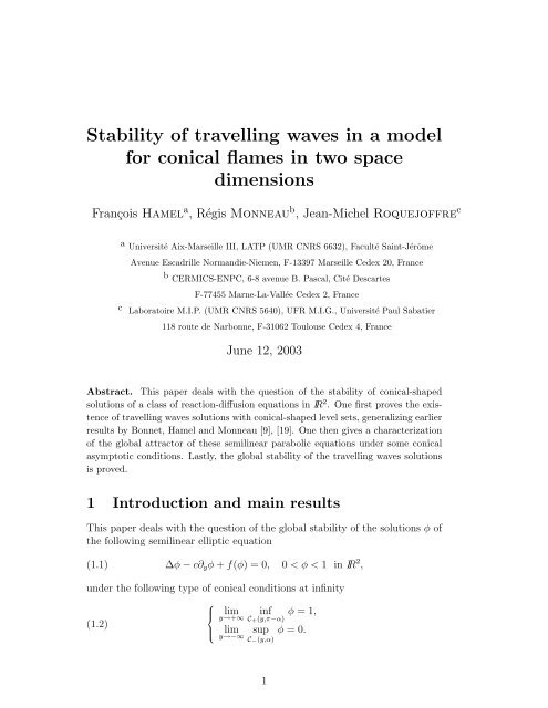
Figure 1: Upper and lower cones<br />
Throughout the paper, the notation ∂ y φ (as well as φ y ) means the partial<br />
<strong>de</strong>rivative of the function φ with respect to the variable y. For any y 0 ∈ IR<br />
and any 0 ≤ β ≤ π, the lower and upper cones C ± (y 0 , β) are <strong>de</strong>fined by<br />
C ± (y 0 , β) = {(x, y) = (0, y 0 ) + ρ(cos ϕ, sin ϕ), ρ ≥ 0, |ϕ ∓ π/2| ≤ β}.<br />
We also use the following notation : for a function v of the 2D real variable<br />
(x, y), and for (a, b) ∈ IR 2 , we <strong>de</strong>note by τ a,b v the function<br />
τ a,b v : (x, y) ↦→ v(x + a, y + b).<br />
Another way of formulating the question of the stability of the solutions φ<br />
of (1.1-1.2) is to ask the question of the convergence to the travelling fronts<br />
φ(x, y + ct), or to some translates of them, for the solutions u(t, x, y) of the<br />
Cauchy problem<br />
{<br />
ut = ∆u + f(u), t > 0, (x, y) ∈ IR 2 ,<br />
(1.3)<br />
u(0, x, y) = u 0 (x, y) given, 0 ≤ u 0 ≤ 1<br />
where u 0 is close, in some sense to be <strong>de</strong>fined later, to a translate τ a,b φ of a<br />
solution φ of (1.1-1.2).<br />
The function f is assumed to be of class C 1,δ in [0, 1] (for some δ > 0) and<br />
to have the following profile :<br />
(1.4)<br />
∃ θ ∈ (0, 1), f = 0 on [0, θ] ∪ {1}, f > 0 on (θ, 1) and f ′ (1 − ) < 0.<br />
For mathematical convenience, we extend f by 0 outsi<strong>de</strong> [0, 1]. Notice that,<br />
from standard elliptic estimates, any classical solution φ of (1.1) is actually of<br />
class C 2,µ (IR 2 ) for any µ ∈ [0, 1).<br />
Equation (1.1) arises in mo<strong>de</strong>ls of equidiffusional premixed Bunsen flames.<br />
The function u is a normalized temperature and its level sets represent the<br />
profile of a conical-shaped Bunsen flame coming out of a thin elongated Bunsen<br />
burner (see Buckmaster and Ludford [12], Joulin [24], Sivashinsky [38],<br />
Williams [40]). The temperature of the unburnt gases is close to 0 and that<br />
of the burnt gases is close to 1, the hot zone being above the fresh zone. The<br />
real θ is called an ignition temperature, below which no reaction happens. The<br />
real c is the speed of the gases at the exit of the burner. Since the shape of the<br />
Bunsen flames is invariant with respect to the size of the Bunsen burner, one<br />
way of mo<strong>de</strong>lling these conical flames consists in setting equation (1.1) in the<br />
whole plane IR 2 together with asymptotic conical conditions of the type (1.2).<br />
The angle 2α then stands for the aperture of the tip of the flame.<br />
In the onedimensional case, equation (1.1) and conditions at infinity (1.2)<br />
reduce to the ordinary differential equation<br />
{<br />
φ<br />
′′<br />
0 − c 0 φ ′ 0 + f(φ 0 ) = 0<br />
(1.5)<br />
φ 0 (−∞) = 0, φ 0 (+∞) = 1.<br />
2
It is well known (Aronson, Weinberger [2], Berestycki, Nicolaenko, Scheurer<br />
[6], Kanel’ [25]) that there exists a unique solution (c 0 , φ 0 ) of (1.5) such that<br />
φ 0 (0) = θ (the solutions of (1.5) are actually unique up to translation). Besi<strong>de</strong>s,<br />
the speed c 0 is positive and the function φ 0 is increasing. The function φ 0 (y) is<br />
also a solution of the two-dimensional problem (1.1-1.2) in the particular case<br />
α = π/2.<br />
In the two-dimensional case with α ≠ π/2, the existence of solutions φ of<br />
(1.1-1.2) was proved by Hamel and Monneau [19] for some angles α ∈ (0, π/2)<br />
and some functions f satisfying (1.4) un<strong>de</strong>r some additional assumptions (see<br />
Theorem 1.8 in [19]). Existence of solutions of (1.1) un<strong>de</strong>r some conical conditions<br />
weaker than (1.2) was also proved by Bonnet and Hamel (see Theorem<br />
1.1 in [9]).<br />
The first result of this paper is to establish the existence of solutions of<br />
(1.1-1.2) for any angle α ∈ (0, π/2] and for any function f satisfying (1.4) :<br />
Theorem 1.1 (Existence) For every angle α ∈ (0, π/2] and for every function<br />
f satisfying (1.4), there exists a solution φ to (1.1-1.2), with c = c 0 / sin α.<br />
Furthermore, it follows from Theorem 1.7 in [19] that the solutions (c, φ)<br />
of (1.1-1.2) are unique, in the sense that c is unique, and φ up to a translation<br />
in (x, y). The speed c is necessarily equal to c = c 0 / sin α. Besi<strong>de</strong>s, any<br />
solution φ satisfies the following properties : 1) there exists a real x 0 such<br />
that φ is symmetric with respect to the vertical line {x = x 0 }, 2) for any<br />
λ ∈ (0, 1), the level set {φ(x, y) = λ} has two asymptots parallel to the halflines<br />
{y = − cot α|x|, x ≥ 0} and {y = − cot α|x|, x ≤ 0}, 3) there exist<br />
two reals t ± such that for any sequence x n → ±∞, the functions φ n (x, y) =<br />
φ(x + x n , y − |x n | cot α) go to the planar fronts φ 0 (±x cos α + y sin α + t ± )<br />
as x n → ±∞ in C 2 loc(IR 2 ). The last two properties mean that any solution<br />
φ is asymptotically conical-shaped far away from the origin : namely, φ is<br />
asymptotically planar and asymptotically equal to two translates of the planar<br />
front φ 0 in the two directions of angle α with respect to the vector −e 2 =<br />
(0, −1).<br />
The formula c = c 0 / sin α, which actually follows from earlier results of<br />
Bonnet and Hamel [9], and had already been used in several papers (see e.g.<br />
Lewis, Von Elbe [28], Sivashinsky [38], Williams [40]), is very natural. In<strong>de</strong>ed,<br />
any solution φ of (1.1-1.2) gives rise to a solution u(t, x, y) = φ(x, y +ct) of the<br />
evolution problem (1.3) with u 0 = φ. The planar speed c 0 is now nothing else<br />
than the projection on the directions (± cos α, − sin α) of the vertical speed c<br />
of the curved front φ(x, y + ct) moving downwards. The speed c 0 is the speed<br />
of two planar waves moving in the directions (± cos α, − sin α) perpendicular<br />
to the half-lines making an angle α with the vertical axis.<br />
Remark 1.2 1. The dimension 2 is quite different from other dimensions<br />
since, as soon as N ≥ 3, there is no solution of problem (1.1) in IR N , with<br />
α < π/2 and conical conditions of the type (1.2) (see [19]). But the possible<br />
3
existence of solutions of (1.1) in IR N un<strong>de</strong>r some weaker conical conditions is<br />
still open in dimensions N ≥ 3.<br />
2. It was also proved in [19] that no solution of (1.1-1.2) exists whenever<br />
α ∈ (π/2, π), in dimensions 2 and higher.<br />
Whereas there are many papers <strong>de</strong>aling with the stability of the travelling<br />
fronts for one-dimensional equations of the type (1.5) with various types of<br />
nonlinearities f (see e.g. [2], [10], [17], [25], [36], [37]), or for wrinkled travelling<br />
fronts of multidimensional equations in infinite cylin<strong>de</strong>rs (see [4] and [8] for the<br />
existence and uniqueness results, and[5], [29], [33], [34], [35] for the stability<br />
results), or lastly for planar fronts in the whole space (see [27], [41]), nothing<br />
seems to be known about the stability of the solutions of two-dimensional<br />
problem (1.1) un<strong>de</strong>r conical conditions of the type (1.2), for α < π/2. As<br />
already emphasized, the travelling fronts φ(x, y + ct) are special time-global<br />
solutions of (1.3) satisfying, at each time, the conical conditions (1.2) in the<br />
frame moving downwards with speed c = c 0 / sin α. Therefore, the question of<br />
the global stability of these travelling waves and the question of the asymptotic<br />
behaviour for large time of the solutions of the Cauchy problem (1.3) starts<br />
from the study of the global attractor of equation (1.3) un<strong>de</strong>r conical conditions<br />
of the type (1.2) in a frame moving downwards with speed c.<br />
The next theorem states that the travelling waves are the only time-global<br />
solutions of (1.3) satisfying such conical conditions.<br />
Theorem 1.3 (Liouville type result) Let α ∈ (0, π/2] and 0 ≤ u(t, x, y) ≤ 1<br />
solve the equation<br />
(1.6)<br />
u t = ∆u + f(u), (x, y) ∈ IR 2<br />
with t ∈ (−∞, +∞) and f satisfying (1.4), and assume that<br />
(1.7)<br />
⎧<br />
⎪⎨<br />
⎪⎩<br />
lim<br />
y 0 →−∞<br />
lim<br />
y 0 →+∞<br />
sup u(t, x, y − ct) = 0<br />
t∈IR, y≤y 0 −|x| cot α<br />
u(t, x, y − ct) = 1.<br />
inf<br />
t∈IR, y≥y 0 −|x| cot α<br />
Then there exists a couple (h, k) ∈ IR 2 such that u(t, x, y) = τ h,k φ(x, y + ct)<br />
for all (t, x, y) ∈ IR × IR 2 , where φ is given by Theorem 1.1.<br />
Since φ(x, y) → 0 (resp. → 1) uniformly as y + |x| cot α → −∞ (resp.<br />
y + |x| cot α → +∞), the following corollary holds :<br />
Corollary 1.4 Let 0 ≤ u(t, x, y) ≤ 1 be a solution of (1.6); assume the existence<br />
of two couples (a 1 , b 1 ) and (a 2 , b 2 ) ∈ IR 2 for which τ a1 ,b 1<br />
φ(x, y + ct) ≤<br />
u(t, x, y) ≤ τ a2 ,b 2<br />
φ(x, y + ct) for all (t, x, y) ∈ IR 3 . Then the conclusion of<br />
Theorem 1.3 holds.<br />
The i<strong>de</strong>a for proving Theorem 1.3 is based on a sliding method (see [7])<br />
in the variable t and some versions of the maximum principle for parabolic<br />
4
equations in unboun<strong>de</strong>d domains. Similar methods were used in [35] and [3]<br />
to get some monotonicity results for the solutions of some semilinear parabolic<br />
equations in various domains.<br />
Theorem 1.3 especially implies the following<br />
Theorem 1.5 (Convergence of a subsequence to a travelling wave) Let φ be a<br />
solution of (1.1-1.2) for α ∈ (0, π/2] with assumptions (1.4) on f. Let u(t, x, y)<br />
be a solution of the Cauchy problem (1.3) such that<br />
⎧<br />
⎨ u 0 ≤ φ in IR 2<br />
(1.8)<br />
⎩ lim inf u<br />
y 0<br />
0(x, y) > θ.<br />
→+∞ y≥y 0 −|x| cot α<br />
Then, for every sequence t n → +∞, there exist a subsequence t n ′<br />
(a, b) ∈ IR 2 such that<br />
→ +∞ and<br />
u(t n ′ + t, x, y − ct n ′ − ct) → φ(x + a, y + b) as n ′ → +∞<br />
locally uniformly in (t, x, y) ∈ IR 3 .<br />
A consequence of this result is that, if u 0 satisfies (1.8) and if ω(u 0 ) is the<br />
ω-limit set of u 0 for the semi-group S(t) given by (1.3), then ω(u 0 ) is ma<strong>de</strong> up<br />
of travelling waves. Condition (1.8) is especially satisfied when u 0 lies between<br />
two translates of a solution φ of (1.1-1.2). But, even un<strong>de</strong>r condition (1.8), the<br />
ω-limit set ω(u 0 ) of u 0 may well be a continuum, and one may ask for sufficient<br />
conditions for ω(u 0 ) to be a singleton. This is the goal of Theorem 1.6 below.<br />
Before stating this result, let us first introduce some notations. Denote by<br />
UC(IR 2 ) the space of all boun<strong>de</strong>d uniformly continuous functions from IR 2 to<br />
IR. We fix a C ∞ function g : IR → IR such that g(x) = |x| for |x| large enough.<br />
For ρ > 0, we set<br />
−ρ(g(x) sin α−y cos α)<br />
(1.9)<br />
q(x, y) = e<br />
and<br />
G ρ = {w ∈ UC(IR 2 ),<br />
The space G ρ is a Banach space with the norm<br />
lim sup |w(x, y)| = 0, w/q ∈ L ∞ (IR 2 )}.<br />
|(x,y)|→+∞<br />
‖w‖ Gρ = ‖w‖ L ∞ (IR 2 ) + ‖w/q‖ L ∞ (IR 2 ).<br />
Theorem 1.6 (Stability result) Choose α ∈ (0, π/2) and let f satisfy (1.4).<br />
Let u(t, x, y) be a solution of the Cauchy problem (1.3) with initial datum<br />
u 0 ∈ UC(IR 2 ) such that 0 ≤ u 0 ≤ 1. Assume the existence of ρ 0 ,<br />
√<br />
C 0 > 0 and of<br />
a solution φ of (1.1-1.2) such that |u 0 (x, y) − φ(x, y)| ≤ C 0 e −ρ 0 x 2 +y 2 in IR 2 .<br />
Also assume that there exists (a, b) ∈ IR 2 such that u 0 ≤ τ a,b φ in IR 2 .<br />
Then there are four constants T ≥ 0, K ≥ 0, ω > 0 and ρ > 0, such that<br />
∀t ≥ T, ‖u(t, x, y − ct) − φ(x, y)‖ Gρ ≤ Ke −ωt .<br />
5
Un<strong>de</strong>r the above assumptions, it especially follows that u(t, ·, · − ct) converges<br />
to φ uniformly √ in IR 2 , and exponentially in time. Notice also that if<br />
|u 0 − φ| ≤ C 0 e −ρ 0 x 2 +y 2<br />
in IR 2 for some solution φ of (1.1-1.2), then u 0 and φ<br />
have the same limits along the lines y = −|x| cot α as x → ±∞, whence such<br />
a φ, if any, is unique.<br />
Notice that Theorem 1.6 holds especially if u 0 ∈ UC(IR 2 ) is such that, say,<br />
0 ≤ u 0 < 1 and if there exists a solution φ of (1.1-1.2) such that u 0 − φ has<br />
compact support.<br />
Lastly, the following theorem holds :<br />
Theorem 1.7 Let α ∈ (0, π/2), and f satisfy (1.4). Let 0 ≤ u(t, x, y) ≤ 1<br />
be a solution of the Cauchy problem (1.3) with u 0 boun<strong>de</strong>d in C 1 (IR 2 ) and<br />
0 ≤ u 0 ≤ 1. Assume that lim y→+∞ inf C+ (y,π−α) u 0 > θ and that there exists a<br />
solution φ of (1.1-1.2) such that u 0 ≤ φ in IR 2 . Also assume that for some<br />
ρ 0 > 0<br />
|∂ eα u 0 (x, y)| ≤ Ce ρ 0(y sin α−x cos α) , |∂ e ′ α<br />
u 0 (x, y)| ≤ Ce ρ 0(y sin α+x cos α)<br />
for all (x, y) ∈ IR 2 , where<br />
(1.10)<br />
e α = (sin α, − cos α) and e ′ α = (− sin α, − cos α).<br />
Then the function u(t, ·, · − ct) converges uniformly in IR 2 , as t → +∞, to<br />
a solution φ ′ of (1.1-1.2).<br />
Remark 1.8 The convergence phenomenon is really governed by the behaviour<br />
of the initial datum when the space variable becomes infinite along the directions<br />
e α and e ′ α. In that sense, the situation is similar to the KPP situation ; see<br />
[29]. It may well happen that, if the initial datum u 0 has no limit in the e α<br />
and e ′ α directions, its ω-limit is ma<strong>de</strong> up of a continuum of waves (see [15]).<br />
Let us mention here similar stability results were obtained by Ninomiya<br />
and Taniguchi [32] for curved fronts in singular limits for Allen-Cahn bistable<br />
equations. Existence of smooth solutions of problem (1.1-1.2) with bistable<br />
nonlinearity f was obtained by Fife [16] for angles α < π/2 close to π/2.<br />
Conical-shaped and more general curved fronts also exist for the Fisher-KPP<br />
equation, with concave nonlinearity f (see [11], [21]). Other stability results<br />
were also obtained by Michelson [31] for Bunsen fronts solving the Kuramoto-<br />
Sivashinsky equation, in some asymptotic regimes. Formal stability results in<br />
the nearly equidiffusional case were also given in [30].<br />
The plan of the paper is the following. Section 2 is <strong>de</strong>voted to the proof<br />
of the existence of travelling waves with the conical conditions at infinity. In<br />
Section 3, we prove that global solutions - i.e. <strong>de</strong>fined for all t ∈ IR - are<br />
travelling wave solutions. In or<strong>de</strong>r to prove Theorem 1.6, we present a local<br />
stability result in Section 4 ; combined to Section 3, this implies the global<br />
stability : this last item will be treated in Section 5.<br />
6
2 Existence of travelling waves solutions<br />
2.1 Proof of Theorem 1.1<br />
Let α ∈ (0, π/2] be given. We are looking for a solution φ of (1.1), i.e.<br />
∆φ − c∂ y φ + f(φ) = 0, 0 < φ < 1 in IR 2<br />
with c = c 0 / sin α, satisfying the conditions (1.2) at infinity, i.e.<br />
⎧<br />
⎪⎨<br />
⎪⎩<br />
lim<br />
y 0 →+∞<br />
lim<br />
y 0 →−∞<br />
inf<br />
y≥y 0 −|x| cot α<br />
sup<br />
y≤y 0 −|x| cot α<br />
φ(x, y) = 1<br />
φ(x, y) = 0<br />
The strategy to prove Theorem 1.1 is to build a solution φ between a sub- and<br />
a supersolution in the whole plane IR 2 .<br />
We perform the proof in three steps.<br />
Step 1 : Construction of a subsolution. A natural candidate for a subsolution<br />
is the following function :<br />
where<br />
φ(x, y) = φ 0 ((y − γ 0 (x)) sin α),<br />
γ 0 (x) = − 1<br />
c 0 sin α ln(cosh(x c 0 cos α)),<br />
and φ 0 is the solution of the one-dimensional problem (1.5) satisfying φ 0 (0) = θ.<br />
It can easily be checked (see also [19] where such subsolutions were used) that<br />
φ is a classical subsolution of<br />
∆φ − c∂ y φ + f(φ) =<br />
cos 2 α<br />
cosh 2 (x c 0 cos α) f(φ 0((y − γ 0 (x)) sin α)) ≥ 0 in IR 2 .<br />
Furthermore, φ is a solution of ∆φ − c∂ y φ = 0 in {y ≤ γ 0 (x)}. Notice that<br />
since φ is of class C 2 , it is also a subsolution of ∆φ − c∂ y φ + f(φ) ≥ 0 in the<br />
viscosity sense.<br />
Moreover, the function γ 0 satisfies sup x∈IR |γ 0 (x) + |x| cot α| < +∞. This<br />
implies in particular<br />
(2.1)<br />
lim<br />
sup<br />
y 0 →−∞<br />
{y≤y 0 −|x| cot α}<br />
φ(x, y) = 0<br />
and<br />
(2.2)<br />
lim<br />
inf<br />
y 0 →+∞ {y≥y 0 −|x| cot α}<br />
φ(x, y) = 1.<br />
Step 2 : Construction of a supersolution. On the contrary, the construction of<br />
a supersolution which is above the subsolution is a nontrivial fact, and requires<br />
the use of the solution ψ to an associated free boundary problem.<br />
7
We <strong>de</strong>fine the candidate for the supersolution as :<br />
{<br />
θ ψ(x, y) in Ω := {ψ < 1}<br />
φ(x, y) =<br />
φ 0 (dist((x, y), Ω)) in IR 2 \Ω<br />
where dist <strong>de</strong>notes the eucli<strong>de</strong>an distance function and ψ is the unique (up to<br />
shift) solution to the following free boundary problem (see [20]) :<br />
Theorem 2.1 (A free boundary problem, 1 [20]) For α ∈ (0, π 2 ], c 0 > 0 and<br />
c = c 0 / sin α, there exists a function ψ satisfying<br />
(2.3)<br />
⎧<br />
⎪⎨<br />
⎪⎩<br />
∆ψ − c∂ y ψ = 0 in Ω := {ψ < 1},<br />
0 < ψ ≤ 1 in IR 2 ,<br />
∂ψ<br />
∂n = c 0 on Γ := ∂Ω,<br />
lim sup ψ = 0,<br />
y→−∞<br />
C − (y,α)<br />
ψ = 1 in C + (y 0 , π − α) for some y 0 ∈ IR,<br />
where ∂ψ stands for the normal <strong>de</strong>rivative on Γ of the restriction of ψ to<br />
∂n<br />
Ω. Furthermore, ψ is continuous in IR 2 , the set Γ = ∂Ω is a C ∞ graph<br />
Γ = {y = ϕ(x), x ∈ IR} such that<br />
sup |ϕ(x) + |x| cot α| < +∞,<br />
x∈IR<br />
Ω is the subgraph Ω = {y < ϕ(x)}, the restriction of ψ is C ∞ in Ω, and<br />
|ϕ ′ (x)| ≤ cot α in IR. Lastly, ψ is non<strong>de</strong>creasing in y, even in x and satisfies<br />
∂ x ψ(x, y) ≥ 0 for x ≥ 0, y < ϕ(x).<br />
From Theorem 2.1 and from the <strong>de</strong>finition of γ 0 , it is easy to see that there<br />
exist two positive constants r 0 and C such that<br />
∀r ≥ r 0 ,<br />
φ r (x, y) := φ(x, y − r) ≤ θ in Ω<br />
and<br />
dist((x, y), Ω)) ≥ −C + (y − γ 0 (x)) sin α in IR 2 \Ω = {ψ = 1}.<br />
Because of (2.1), and from the comparison principles proved in [19], it follows<br />
that φ r ≤ φ in Ω for all r ≥ r 0 and then, by construction of φ, we get that<br />
φ r ≤ φ in IR 2<br />
1 This problem arises in mo<strong>de</strong>ls of equidiffusional premixed Bunsen flames in the limit<br />
of high activation energy. The existence of a solution ψ of problem (2.3) can be obtained<br />
by regularizing approximations, starting from solutions of problems of the type (1.1) with<br />
nonlinearities f ε approximating a Dirac mass at 1.<br />
8
as soon as r ≥ max(r 0 , C/ sin α).<br />
Moreover, notice that the construction of φ implies that<br />
(2.4)<br />
lim<br />
sup<br />
y 0 →−∞<br />
{y≤y 0 −|x| cot α}<br />
φ(x, y) = 0.<br />
We shall prove in Section 2.2 the following result<br />
Proposition 2.2 The function φ is a supersolution of (1.1) in the vicosity<br />
sense.<br />
Step 3 : Existence of a solution. Choose a real number r such that r ≥<br />
max(r 0 , C/ sin α). By using the Perron method for viscosity solutions (see [14]<br />
and H. Ishii [23], Theorem 7.2 page 41), we get the existence of a vicosity<br />
solution φ of ∆φ − c∂ y φ + f(φ) = 0, which satisfies :<br />
0 ≤ φ r ≤ φ ≤ φ ≤ 1 in IR 2 .<br />
Now by the regularity theory for viscosity solutions (see [13]), it follows that<br />
φ is C 2+β (with β > 0), and then φ is a classical solution of (1.1). Finally<br />
φ satisfies the conditions at infinity (1.2) because of (2.2) and (2.4). This<br />
completes the proof of Theorem 1.1.<br />
2.2 Proof of Proposition 2.2<br />
The proof of Proposition 2.2 is based on the following result :<br />
Lemma 2.3 Let ξ be the function <strong>de</strong>fined by<br />
ξ(x, y) = φ −1<br />
0 (θ ψ(x, y)) in Ω = {y ≤ ϕ(x)},<br />
where ψ is the solution to the free boundary problem given by Theorem 2.1.<br />
Then<br />
|∇ξ| ≤ 1 in Ω.<br />
Proof. We have<br />
⎧ (<br />
⎪⎨ ∆ξ + c 0 |∇ξ| 2 − ∂ )<br />
yξ<br />
= 0 in Ω = {ξ < 0},<br />
sin α<br />
⎪⎩ ξ = 0 and ∂ξ = 1 on Γ = ∂{ξ < 0}<br />
∂n<br />
since φ 0 (s) = θe c 0s for all s ≤ 0. A straightforward computation gives, for<br />
v = |∇ξ| 2 :<br />
∆v + b · ∇v = 2|D 2 ξ| 2 ,<br />
where b = 2c 0 ∇ξ − c 0 / sin α e y and e y = (0, 1).<br />
9
We want to prove that v ≤ 1. But v = 1 on Γ and v → 0 uniformly as<br />
d((x, y), Γ) → +∞. From the maximum principle we conclu<strong>de</strong> that<br />
which proves the lemma.<br />
v ≤ sup v = 1,<br />
Γ<br />
Let us now turn to the<br />
Proof of Proposition 2.2. Let us <strong>de</strong>fine<br />
I[u] := ∆u − c∂ y u + f(u).<br />
By construction φ is a classical solution of I[φ] = 0 in the open set Ω = {φ < θ}.<br />
Moreover the gradient of φ is continuous across Γ = ∂{φ < θ}, which is smooth.<br />
Let us now consi<strong>de</strong>r the function ξ(x, y) = φ −1<br />
0 (φ(x, y)), now <strong>de</strong>fined in the<br />
whole plane IR 2 . We have<br />
J[ξ] := I[φ]<br />
(<br />
φ ′ 0(ξ) = ∆ξ + c 0 |∇ξ| 2 − ∂ )<br />
yξ<br />
(2.5)<br />
+ G(ξ) ( 1 − |∇ξ| 2)<br />
sin α<br />
in the viscosity sense in IR 2 , where G(ξ) = f(φ 0 (ξ))/φ ′ 0(ξ) ≥ 0. Because<br />
ξ(x, y) = d((x, y), Γ) in IR 2 \Ω = {ξ ≥ 0}, the following inequality holds in the<br />
viscosity sense :<br />
J[ξ] ≤ H[ξ] := −<br />
K (<br />
1 − Kξ + c 0 1 − n · e )<br />
y<br />
(2.6)<br />
in {y > ϕ(x)},<br />
sin α<br />
and equality holds where ξ is smooth (see Gilbarg, Trudinger [18]). Here<br />
K = K(Y ) and n = n(Y ) are respectively the curvature 2 and the exterior<br />
normal to the set Ω at a point Y = Y (x, y) ∈ Γ where the ball B ξ(x,y) ((x, y))<br />
is tangent to Γ.<br />
On the other hand, on the level set Γ we have |∇ξ| = 1 and because of<br />
Lemma 2.3 we get Dnnξ 2 ≥ 0. Therefore, since I[φ] = 0 in Ω, we <strong>de</strong>duce from<br />
(2.5) that<br />
(<br />
−K(Y ) + c 0 1 − n(Y ) · e )<br />
y<br />
≤ 0 for all Y ∈ Γ.<br />
sin α<br />
Furthermore, observe that the inequality<br />
−K(Y )<br />
1 − K(Y )ξ(x, y) ≤ −K(Y )<br />
holds for all (x, y) ∈ IR 2 \Ω = {ξ ≥ 0}, whatever the sign of K is, un<strong>de</strong>r the<br />
same notations as above for Y .<br />
Therefore, H[ξ] ≤ 0 in IR 2 \Ω and finally J[ξ] ≤ 0 in {y > ϕ(x)} = {ξ > 0}<br />
in the viscosity sense. Hence, I[φ] ≤ 0 in IR 2 in the viscosity sense, which ends<br />
the proof of Proposition 2.2.<br />
2 un<strong>de</strong>r the convention that the curvature of a disk is negative<br />
10
3 Global solutions are travelling waves<br />
This section is <strong>de</strong>voted to the proof of Theorems 1.3 and Theorem 1.5 below,<br />
the latter being a consequence of the former.<br />
One of the main tools in the proof of Theorem 1.3 is the following comparison<br />
principle :<br />
Proposition 3.1 (Comparison principle) Let δ ∈ IR and g : IR → IR be<br />
a Lipschitz-continuous function which is nonincreasing in (−∞, δ]. Let ψ :<br />
IR → IR be a Lipschitz-continuous function. Let v : (t, x, y) ↦→ v(t, x, y) and<br />
v : (t, x, y) ↦→ v(t, x, y) be two boun<strong>de</strong>d and Lipschitz-continuous functions<br />
<strong>de</strong>fined on IR × Ω, where Ω = {y < ψ(x)}. Let κ ∈ IR. Assume that<br />
{<br />
vt ≤ ∆v + κ∂ y v + g(v) in D ′ (IR × Ω)<br />
v t ≥ ∆v + κ∂ y v + g(v) in D ′ (IR × Ω),<br />
v ≤ δ in IR × Ω, v(t, x, ψ(x)) ≤ v(t, x, ψ(x)) for all (t, x) ∈ IR 2 , and<br />
lim<br />
y 0 →−∞<br />
sup (v(t, x, y) − v(t, x, y)) ≤ 0.<br />
t∈IR, y 0 large enough. Let us now <strong>de</strong>fine<br />
ε ∗ = inf {ε > 0, v − ε ′ ≤ v in IR × Ω for all ε ′ ≥ ε}.<br />
By continuity, one can immediately say that v − ε ∗ ≤ v in IR × Ω.<br />
Let us now assume that ε ∗ > 0. There exists then a sequence ε n < →ε ∗ and<br />
a sequence of points (t n , x n , y n ) in IR × Ω such that<br />
v(t n , x n , y n ) − ε n > v(t n , x n , y n ).<br />
Since ε n ≥ ε ∗ /2 > 0 for n large enough, it follows from the assumptions of<br />
Proposition 3.1 that there exist two real numbers 0 < A ≤ B such that<br />
(3.1)<br />
ψ(x n ) − B ≤ y n ≤ ψ(x n ) − A<br />
for n large enough.<br />
Call ψ n (x) = ψ(x + x n ) − y n and let v n and v n the functions <strong>de</strong>fined in<br />
IR × {y ≤ ψ n (x)} by<br />
v n (t, x, y) = v(t + t n , x + x n , y + y n ) and v n (t, x, y) = v(t + t n , x + x n , y + y n ).<br />
Since the functions ψ n are uniformly Lipschitz-continuous, they locally converge,<br />
up to extraction of some subsequence, to a globally Lipschitz-continuous<br />
function ψ ∞ . Similarly, up to extraction of another subsequence, the functions<br />
11
v n and v n converge locally uniformly in IR × {y < ψ ∞ (x)} to two globally<br />
Lipschitz-continuous functions v ∞ and v ∞ , which can be exten<strong>de</strong>d by continuity<br />
on IR × {y = ψ ∞ (x)}. Call<br />
Ω ∞ = {(x, y) ∈ IR 2 , y < ψ ∞ (x)}.<br />
Since v(t, x, ψ(x)) ≤ v(t, x, ψ(x)) for all (t, x) ∈ IR 2 and since v and v are<br />
globally Lipschitz-continuous in IR × Ω, it follows that<br />
v ∞ (t, x, ψ ∞ (x)) ≤ v ∞ (t, x, ψ ∞ (x))<br />
for all (t, x) ∈ IR 2 .<br />
By passage to the limit, the functions v ∞ and v ∞ satisfy<br />
{<br />
(v∞ ) t ≤ ∆v ∞ + κ∂ y v ∞ + g(v ∞ ) in D ′ (IR × Ω ∞ )<br />
(v ∞ ) t ≥ ∆v ∞ + κ∂ y v ∞ + g(v ∞ ) in D ′ (IR × Ω ∞ )<br />
and v ∞ − ε ∗ ≤ v ∞ in IR × Ω ∞ . On the other hand, ψ ∞ (0) ≥ A > 0 from (3.1),<br />
and v ∞ (0, 0, 0)−ε ∗ = v ∞ (0, 0, 0). Lastly, v ∞ −ε ∗ ≤ v ∞ ≤ δ in IR×Ω ∞ and the<br />
function g was assumed to be nonincreasing in (−∞, δ]. Hence, g(v ∞ − ε ∗ ) ≥<br />
g(v ∞ ) in IR × Ω ∞ .<br />
Therefore, the function w := v ∞ −ε ∗ −v ∞ is a boun<strong>de</strong>d, globally Lipschitzcontinuous<br />
and nonpositive function in IR×Ω ∞ , vanishing at the point (0, 0, 0)<br />
and satisfying<br />
w t ≤ ∆w + κ∂ y w + γ(t, x, y)w in D ′ (IR × Ω ∞ ),<br />
where γ is globally boun<strong>de</strong>d function (here we use the fact that g is globally<br />
Lipschitz-continuous). The strong parabolic maximum principle then implies<br />
that w(t, x, y) = 0, i.e. v ∞ (t, x, y) − ε ∗ = v ∞ (t, x, y), for all t ≤ 0 and (x, y) ∈<br />
Ω ∞ . But the positivity of ε ∗ contradicts the fact that v ∞ ≤ v ∞ on IR × ∂Ω ∞ .<br />
As a conclusion, ε ∗ = 0 and v ≤ v in IR × Ω.<br />
Remark 3.2 The above comparison principle is a version of a parabolic maximum<br />
principle for time-global solutions in an unboun<strong>de</strong>d space-domain. This<br />
comparison principle actually holds the same way in any space-dimension for<br />
more general second-or<strong>de</strong>r parabolic operators with smooth coefficients <strong>de</strong>pending<br />
on time and space and a non-linearity g(t, x 1 , · · · , x N , u) satisfying the same<br />
monotonicity assumption with respect to u as in Proposition 3.1.<br />
Let us now turn to the<br />
Proof of Theorem 1.3. Un<strong>de</strong>r the assumptions of Theorem 1.3, the function<br />
v <strong>de</strong>fined in IR 3 by v(t, x, y) := u(t, x, y − ct) is such that 0 ≤ v ≤ 1 and it<br />
solves<br />
(3.2)<br />
v t = ∆v − c∂ y v + f(v).<br />
12
From standard parabolic estimates, the function v is globally Lipschitz-continuous<br />
with respect to all variables (t, x, y). Furthermore, v satisfies<br />
(3.3)<br />
⎧<br />
⎪⎨<br />
⎪⎩<br />
lim<br />
y 0 →−∞<br />
lim<br />
y 0 →+∞<br />
sup v(t, x, y) = 0<br />
t∈IR, y≤y 0 −|x| cot α<br />
v(t, x, y) = 1.<br />
inf<br />
t∈IR, y≥y 0 −|x| cot α<br />
We shall now prove that v is actually in<strong>de</strong>pen<strong>de</strong>nt of t. That will imply<br />
that v = v(x, y) is a solution of (1.1-1.2) (notice that from the strong maximum<br />
principle, one then has 0 < v < 1). From Theorem 1.1 and from the uniqueness<br />
results in [19], it will follow that v = τ a,b φ in IR 2 , for some pair (a, b) ∈ IR 2 .<br />
Fix now any real number t 0 . For s ∈ IR, call w s the function <strong>de</strong>fined in IR 3<br />
by<br />
w s (t, x, y) = v(t + t 0 , x, y + s).<br />
The function w s is a solution of (3.2) as well.<br />
From the assumptions on f, there exists ρ > 0 such that θ ≤ 1 − ρ and f is<br />
nonincreasing on the interval [1 − ρ, +∞). Remember also that f is i<strong>de</strong>ntically<br />
equal to 0 on (−∞, θ]. From (3.3), there exists A > 0 such that<br />
{<br />
v(t, x, y) ≥ 1 − ρ for all t ∈ IR, y ≥ A − |x| cot α<br />
v(t, x, y) ≤ θ for all t ∈ IR, y ≤ −A − |x| cot α.<br />
Choose any s ≥ 2A and observe that<br />
w s (t, x, −A − |x| cot α) = v(t + t 0 , x, s − A − |x| cot α)<br />
≥ 1 − ρ ≥ θ ≥ v(t, x, −A − |x| cot α)<br />
for all (t, x) ∈ IR 2 . It is then immediate to check that all the assumptions of<br />
Proposition 3.1 are satisfied with g = f, δ = θ, ψ(x) = −A − |x| cot α, κ = −c,<br />
v = v, v = w s . Therefore,<br />
w s (t, x, y) ≥ v(t, x, y) for all t ∈ IR and y ≤ −A − |x| cot α.<br />
Similarly, the assumptions of Proposition 3.1 are also satisfied with the choices<br />
g(τ) = −f(1−τ), δ = ρ, ψ(x) = A+|x| cot α, κ = c, v(t, x, y) = 1−w s (t, x, −y)<br />
and v(t, x, y) = 1 − v(t, x, −y). Therefore, v(t, x, y) ≤ v(t, x, y) for all t ∈ IR<br />
and y ≤ A + |x| cot α, which means that<br />
v(t, x, y) ≤ w s (t, x, y) for all t ∈ IR and y ≥ −A − |x| cot α.<br />
As a consequence, one has v ≤ w s in IR 3 for all s ≥ 2A. Let us now <strong>de</strong>fine<br />
s ∗ = inf {s > 0, v ≤ w τ in IR 3 for all τ ≥ s}.<br />
By continuity, one has v ≤ w s∗ . Let us assume by contradiction that s ∗ > 0.<br />
One shall consi<strong>de</strong>r two cases, namely whether the infimum of w s∗ −v is positive<br />
or zero on the strip<br />
S = {(t, x, y) ∈ IR 3 , |y + |x| cot α| ≤ A}.<br />
13
Case 1 : inf S (w s∗ − v) > 0. Since the function v, as well as w s∗ , is globally<br />
Lipschitz-continuous, there exists η 0 ∈ (0, s ∗ ) such that w s∗ −η ≥ v in S for all<br />
η ∈ [0, η 0 ]. Choose any η ∈ [0, η 0 ]. Since s ∗ − η ≥ 0, one has w s∗ −η (t, x, y) ≥<br />
1 − ρ for all t ∈ IR and y ≥ A − |x| cot α. It also follows from the choice of η<br />
that<br />
w s∗ −η (t, x, A − |x| cot α) ≥ v(t, x, A − |x| cot α)<br />
for all (t, x) ∈ IR 2 (since (t, x, A − |x| cot α) ∈ ∂S for all (t, x) ∈ IR 2 ). As<br />
above, it is straightforward to check that Proposition 3.1 implies that<br />
w s∗ −η (t, x, y) ≥ v(t, x, y) for all t ∈ IR and y ≥ A − |x| cot α.<br />
Similarly, it can also be <strong>de</strong>duced that<br />
w s∗ −η (t, x, y) ≥ v(t, x, y) for all t ∈ IR and y ≤ −A − |x| cot α.<br />
Putting all the preceeding facts together, one conclu<strong>de</strong>s that w s∗ −η ≥ v in<br />
IR 3 for all η ∈ [0, η 0 ]. This is contradiction with the minimality of s ∗ , since<br />
η 0 > 0. Therefore, case 1 is ruled out.<br />
Case 2 : inf S (w s∗ − v) = 0. There exists then a sequence (t n , x n , y n ) such<br />
that t n ∈ IR, −A − |x n | cot α ≤ y n ≤ A − |x n | cot α and<br />
w s∗ (t n , x n , y n ) − v(t n , x n , y n ) → 0 as n → +∞.<br />
Call v n (t, x, y) = v(t + t n , x + x n , y + y n ). Each function v n is a solution of<br />
(3.2) and ranges in [0, 1]. From standard parabolic estimates, the functions<br />
v n converge locally uniformly, up to extraction of some subsequence, to a<br />
global solution v ∞ of (3.2) such that 0 ≤ v ∞ ≤ 1. Furthermore, v ∞ (t 0 , 0, s ∗ ) =<br />
v ∞ (0, 0, 0). Therefore, the function z(t, x, y) := v ∞ (t+t 0 , x, y+s ∗ )−v ∞ (t, x, y),<br />
which is nonnegative since v ≤ w s∗ , vanishes at (0, 0, 0) and is a global boun<strong>de</strong>d<br />
solution of<br />
z t = ∆z − c∂ y z + γ(t, x, y)z<br />
for some boun<strong>de</strong>d function γ (here we use the fact that f is globally Lipschitzcontinuous).<br />
The strong maximum principle for t ≤ 0 and the uniqueness of<br />
the Cauchy problem for the above equation then imply that z(t, x, y) = 0 for<br />
all (t, x, y) ∈ IR 3 . As a consequence,<br />
(3.4)<br />
v ∞ (t + nt 0 , x, y + ns ∗ ) = v ∞ (t, x, y)<br />
for all (t, x, y) ∈ IR 3 and n ∈ Z.<br />
Furthermore, from the <strong>de</strong>finitions of (t n , x n , y n ), one of the following three<br />
cases occur up to extraction of some subsequence : (i) the sequence (x n , y n ) is<br />
boun<strong>de</strong>d, (ii) x n → −∞, or (iii) x n → +∞.<br />
If case (i) occurs, then (3.3) holds for v ∞ .<br />
function v ∞ satisfies<br />
⎧<br />
⎪⎨<br />
⎪⎩<br />
lim<br />
y 0 →−∞<br />
lim<br />
y 0 →+∞<br />
sup v ∞ (t, x, y) = 0<br />
t∈IR, y≤y 0 +x cot α<br />
inf v ∞(t, x, y) = 1.<br />
t∈IR, y≥y 0 +x cot α<br />
14<br />
If case (ii) occurs, then the
Lastly, if case (iii) occurs, then v ∞ satisfies<br />
⎧<br />
⎪⎨<br />
⎪⎩<br />
lim<br />
y 0 →−∞<br />
lim<br />
y 0 →+∞<br />
sup v ∞ (t, x, y) = 0<br />
t∈IR, y≤y 0 −x cot α<br />
inf v ∞(t, x, y) = 1.<br />
t∈IR, y≥y 0 −x cot α<br />
In each of the three cases (i), (ii) or (iii), one gets a contradiction with property<br />
(3.4). Therefore case 2 is ruled out too.<br />
As a conclusion, the assumption s ∗ > 0 is impossible, whence<br />
v(t, x, y) ≤ w 0 (t, x, y) = v(t + t 0 , x, y)<br />
for all (t, x, y) ∈ IR 3 . Since t 0 is arbitrary in IR, one conclu<strong>de</strong>s that v does not<br />
<strong>de</strong>pend on the variable t. As already emphasized, that completes the proof of<br />
Theorem 1.3.<br />
Let us now turn to the<br />
Proof of Theorem 1.5. The functions v n (t, x, y) = u(t n + t, x, y − ct n − ct)<br />
solve<br />
(3.5)<br />
∂ t v n = ∆v n − c∂ y v n + f(v n )<br />
for t > −t n . Furthermore, since φ is a solution of (1.1), the maximum principle<br />
implies that<br />
v n (t, x, y) ≤ φ(x, y)<br />
for all (x, y) ∈ IR 2 and for all t ≥ −t n . On the other hand, because of the<br />
second inequality in (1.8) and because u 0 is nonnegative, there exist η ∈ (θ, 1]<br />
and s 0 ∈ IR such that<br />
∀(x, y) ∈ IR 2 , u 0 (x, y) ≥ max(H(±x cos α + y sin α + s 0 )),<br />
where H(s) = 0 if s < 0 and H(s) = η if s ≥ 0. Therefore,<br />
∀t ≥ −t n , ∀(x, y) ∈ IR 2 ,<br />
v n (t, x, y) ≥ max(v + (t n + t, x, y), v − (t n + t, x, y)),<br />
where the functions v ± solve equation (3.5) with initial conditions v ± (0, x, y) =<br />
H(±x cos α + y sin α + s 0 ). Consi<strong>de</strong>r the function v + . Since equation (3.5) is<br />
invariant up to translation and since v + (0, ·, ·) only <strong>de</strong>pends on the variable<br />
s = x cos α + y sin α, so does v + (t, ·, ·) at any time t ≥ 0. Therefore, v + (t, x, y)<br />
can be written as v + (t, x, y) = V + (t, s) where V + solves<br />
{<br />
∂ t V + = ∂sV 2 + − c 0 ∂ s V + + f(V + )<br />
V + (0, s) = H(s + s 0 ).<br />
A result of Kanel’ [25], [26] (see also Roquejoffre [35]) yields the convergence<br />
of V + (t, s) to φ 0 (s + s 1 ) uniformly in s ∈ IR as t → +∞, for some s 1 ∈ IR,<br />
where φ 0 is the solution of (1.5) such that, say, φ 0 (0) = θ. By symmetry in the<br />
15
x-variable, it follows that v − (t, x, y) → φ 0 (s ′ + s 1 ) uniformly in (x, y) ∈ IR 2 as<br />
t → +∞, where s ′ = −x cos α + y sin α. Consequently,<br />
∀(t, x, y) ∈ IR 3 ,<br />
lim inf v n(t, x, y) ≥ max(φ 0 (±x cos α + y sin α + s 1 )).<br />
n→+∞<br />
Eventually, from standard parabolic estimates, there exists a subsequence<br />
n ′ → +∞ such that the functions v n ′ converge locally uniformly in IR × IR 2 to<br />
a classical solution v(t, x, y) of v t = ∆v − cv y + f(v) such that<br />
max(φ 0 (±x cos α + y sin α + s 1 )) ≤ v(t, x, y) ≤ φ(x, y)<br />
for all (t, x, y) ∈ IR 3 .<br />
The function u(t, x, y) = v(t, x, y + ct) then satisfies (1.6) and (1.7). Theorem<br />
1.3 yields that u(t, x, y) = φ(x + a, y + b + ct) for some (a, b) ∈ IR 2 and for<br />
all (t, x, y) ∈ IR × IR 2 . Therefore, v(t, x, y) = φ(x + a, y + b) and the conclusion<br />
of Theorem 1.5 follows.<br />
4 Local stability<br />
The goal of this section is to prove the following stability result :<br />
Theorem 4.1 (Local Stability) Let α ∈ (0, π/2) and f satisfy (1.4). Let<br />
u(t, x, y) be a solution of the Cauchy problem (1.3). There exists ρ > 0 (one<br />
may choose ρ = c 0 cot α) such that the following holds : for any ρ ∈ (0, ρ),<br />
there is ε > 0 such that if 0 ≤ u 0 ≤ 1, u 0 ∈ UC(IR 2 ), and ‖u 0 − φ‖ Gρ ≤ ε for<br />
some solution φ of (1.1-1.2), then there are two constants K ≥ 0 and ω > 0<br />
such that<br />
∀t ≥ 0, ‖u(t, ·, · − ct) − φ(·, ·)‖ Gρ ≤ Ke −ωt .<br />
The object to study is the linearized operator around a wave solution φ :<br />
Lv = −∆v + c∂ y v − f ′ (φ)v.<br />
In the whole section, we choose the (unique) wave φ solving (1.1-1.2) such<br />
that :<br />
φ(x, y) = φ(−x, y), φ(0, 0) = θ.<br />
Proposition 4.2 (No eigenvalue with negative real part) Let ρ > 0 and u ∈<br />
C(IR 2 , C) be a classical solution of Lu = λu such that Re(u), Im(u) ∈ G ρ .<br />
• If Re(λ) < 0, then u = 0.<br />
• If Re(λ) = 0, then there is C > 0 such that<br />
|u| ≤ Cφ y in IR 2 .<br />
16
Proof. We wish to follow the i<strong>de</strong>a in [5]. The result is obtained by proving<br />
first that u <strong>de</strong>cays faster than any <strong>de</strong>rivative of the wave, then to conclu<strong>de</strong><br />
with the aid of the parabolic equation<br />
(4.1)<br />
U t + LU = 0,<br />
U(0) = Re(u).<br />
This first part of the programme does not seem to be done as easily as in<br />
[5], due to the lack of precise boundaries where to apply an exact boundary<br />
condition - hence an evolution equation approach -.<br />
In or<strong>de</strong>r to circumvent the difficulty we directly use equation (4.1) and<br />
construct a Fife-McLeod type super-solution (see [17]) : set<br />
w 0 (x, y) = min(e˜ρ(y sin α−x cos α) , e˜ρ(y sin α+x cos α) ),<br />
where ˜ρ ∈ (0, c 0 ) shall be chosen later. We also set<br />
Ū(t, x, y) = a 0 (t)φ y (x, y) + a 1 (t)γ 1 (x, y) + a 2 (t)w 0 (x, y)γ 2 (x, y).<br />
Define y 1 > 0 and k > 0 such that<br />
(4.2)<br />
∀(x, y) ∈ C + (y 1 , π − α),<br />
f ′ (φ(x, y)) ≤ −k<br />
and choose y 2 < 0 such that<br />
(4.3)<br />
∀(x, y) ∈ C − (y 2 , α), f ′ (φ(x, y)) = 0.<br />
Actually, any negative y 2 works since φ(0, 0) = θ and it is known ([9], [19]) that<br />
φ is nonincreasing in any direction τ = (cos β, sin β) such that −π/2 − α ≤<br />
β ≤ −π/2 + α. The functions γ 1 and γ 2 are required to be in C 2 (IR 2 ) and to<br />
satisfy<br />
• 0 ≤ γ 1 , γ 2 ≤ 1 in IR 2 ;<br />
• γ 1 ≡ 1 in C + (2y 1 , π − α) and γ 1 ≡ 0 in C − (y 1 , α);<br />
• γ 2 ≡ 1 in C − (2y 2 , α) and γ 2 ≡ 0 in C + (y 2 , π − α);<br />
• ∂ x γ 1 (0, y) = ∂ x γ 2 (0, y) ≡ 0.<br />
Then set<br />
LŪ = Ūt + LŪ;<br />
as is now classical we anticipate that ȧ 0 (t) will be nonnegative, and break the<br />
evaluation of LŪ in three parts.<br />
1. (x, y) ∈ C − (2y 2 , α). Then we have, because of (4.3) and because φ y ≥ 0 :<br />
LŪ ≥<br />
(<br />
ȧ 2 (t) + (c˜ρ sin α − ˜ρ 2 )a 2 (t) ) w 0 ,<br />
17
provi<strong>de</strong>d that a 2 (t) is nonnegative. Remember that c sin α = c 0 and set<br />
a 2 (t) = α 2 e −t˜ρ(c 0−˜ρ)<br />
with α 2 > 0 to be chosen later. Observe here that ˜ρ(c 0 − ˜ρ) > 0 since ˜ρ is in<br />
(0, c 0 ).<br />
2. (x, y) ∈ C + (2y 1 , π − α). Then we have, because of (4.2) and provi<strong>de</strong>d that<br />
a 1 (t) is nonnegative :<br />
LŪ ≥ ȧ 1(t) + ka 1 (t),<br />
and we <strong>de</strong>fine<br />
a 1 (t) = α 1 e −kt<br />
with α 1 > 0 to be chosen later.<br />
3. (x, y) ∈ C − (2y 1 , α) ∩ C + (2y 2 , π − α). There is a large constant C 1 > 0 and<br />
a small positive constant ω such that<br />
LŪ ≥ ȧ 0(t)φ y (x, y) − C 1 e −ωt .<br />
Then, because φ y is positive and boun<strong>de</strong>d away from 0 in the region un<strong>de</strong>r<br />
consi<strong>de</strong>ration, there is a large constant C 2 such that we may take<br />
and<br />
a 0 (t) = α 0 − C 2 e −ωt , α 0 > 0,<br />
LŪ ≥ 0 in C −(2y 1 , α) ∩ C + (2y 2 , π − α).<br />
Combining the above steps, and since Re(u) ∈ G ρ , one can choose α 0 , α 1 ,<br />
α 2 large enough and ˜ρ > 0 small enough so that Ū satisfies LŪ ≥ 0 in IR +×IR 2<br />
and Re(u) ≤ Ū(0, .). Then we have :<br />
Re(e −λt u)(t, x, y) ≤ Ū(t, x, y).<br />
We may repeat the argument with −Re(u) so as to obtain a similar lower<br />
bound for Re(e −λt u).<br />
We can now conclu<strong>de</strong> :<br />
• If Re(λ) < 0, assuming u ≠ 0 contradicts the unboun<strong>de</strong>dness of Re(e −λt u).<br />
• If Re(λ) = 0, then we argue similarly with Im(u) and Im(e −λt u) and<br />
we get an upper bound of the type |Im(e −λt u)| ≤ ¯V (t, x, y), where ¯V is<br />
of the same type as Ū. We then only have to let t → +∞ to get that<br />
|u| ≤ Cφ y in IR 2 .<br />
This ends the proof of Proposition 4.2.<br />
The next step is to show that 0 is NOT an eigenvalue of L when L is<br />
restricted to G ρ . We first observe that<br />
L(φ x ) = L(φ y ) = 0,<br />
18
ut neither φ x nor φ y belongs to G ρ since lim inf |x|→+∞ φ x (x, −|x| cot α) and<br />
lim inf |x|→+∞ φ y (x, −|x| cot α) are positive (in<strong>de</strong>ed, φ(x + ξ, y − |ξ| cot α) →<br />
φ 0 (±x cos α + y sin α + t ± ) as ξ → ±∞ in C 2 loc(IR 2 ), for some t ± ∈ IR). 3<br />
Then remark that a function u(x, y) may be <strong>de</strong>composed in an even and<br />
odd part (with respect to x) : u = u 1 + u 2 with<br />
u 1 (x, y) =<br />
u(x, y) + u(−x, y)<br />
, u 2 (x, y) =<br />
2<br />
u(x, y) − u(−x, y)<br />
.<br />
2<br />
Notice also that ∂ x u 1 (0, y) = 0 - provi<strong>de</strong>d u 1 is smooth enough - and that<br />
u 2 (0, y) = 0. This trivial remark implies in fact boundary conditions for u 1<br />
and u 2 on the y-axis if u 1 and u 2 are consi<strong>de</strong>red as functions from the right<br />
half-space that we <strong>de</strong>note IR 2 + = {x > 0}. Notice finally that φ x is odd and φ y<br />
is even (with respect to the x-variable).<br />
On the other hand, the operator L commutes with the reflections with<br />
respect to the y axis. Hence, if a function u in G ρ solves Lu = 0, then both<br />
functions u 1 and u 2 are in G ρ and solve Lu = 0. On the basis of all the above<br />
remarks we have the<br />
Proposition 4.3 (No eigenfunctions in the null space of L) (i). Let ρ > 0<br />
and u ∈ C 2 (IR 2 +) ∩ G ρ solve<br />
(4.4)<br />
Lu = 0 in IR 2 +, u(0, y) = 0.<br />
Then u = 0.<br />
(ii). Let ρ > 0 and u ∈ C 2 (IR 2 +) ∩ G ρ solve<br />
Then u = 0.<br />
Lu = 0 in IR 2 +, u x (0, y) = 0.<br />
We will only prove part (i) of Proposition 4.3, part (ii) being completely<br />
similar and being actually inclu<strong>de</strong>d in the proof of Proposition 4.5 below. The<br />
proof of part (i) will be based on the following<br />
Lemma 4.4 Let ρ > 0 and u ∈ C 2 (IR 2 +) ∩ G ρ satisfy (4.4). Then there is a<br />
constant C > 0 such that<br />
|u| ≤ Cφ x in IR 2 +.<br />
Proof. Argue as in Proposition 4.2, but this time u vanishes at the boundary<br />
{x = 0}, as well as φ x . To circumvent this we <strong>de</strong>fine the supersolution Ū as<br />
Ū(t, x, y) = a 0 (t)φ x (x, y) +<br />
(<br />
)<br />
a 1 (t)γ 1 (x, y) + a 2 (t)w 0 (x, y)γ 2 (x, y) w 1 (x),<br />
3 We have of course t − = t + as soon as φ is symmetric with respect to the x-variable.<br />
19
where w 1 is boun<strong>de</strong>d, increasing and concave, and satisfies moreover w 1 (0) =<br />
w 1(0) ′′ = 0 and w 1 (+∞) = 1. With similar choices for the functions a 0 , a 1 ,<br />
a 2 , w 0 as in Proposition 4.2, one has LŪ ≥ 0 for all t ≥ 0 and (x, y) ∈ IR2 +.<br />
Furthermore, since Lφ x = 0, φ x > 0 in IR + 2 and φ x = 0 on {x = 0}, it<br />
follows from Hopf lemma that φ xx (0, y) > 0 for all y ∈ IR. On the other<br />
hand, the standard elliptic estimates up to the boundary imply that, say,<br />
‖∇u‖ L ∞ ({0≤x≤1, y 0 ≤y≤y 0 +1}) ≤ C 0 ‖u‖ L ∞ ({0≤x≤2, y 0 −1≤y≤y 0 +2}) for some constant<br />
C 0 in<strong>de</strong>pendant of y 0 ∈ IR. Therefore, suitable choices of a 0 , a 1 , a 2 and ˜ρ<br />
guarantee that u(x, y) ≤ Ū(0, x, y) in IR2 +. Hence, u(x, y) ≤ Ū(t, x, y) for all<br />
t ≥ 0 and (x, y) ∈ IR +. 2 Passing to the limit t → +∞ as in Proposition 4.2<br />
leads to u ≤ Cφ x in IR +.<br />
2<br />
The same reasoning with −u completes the proof of Lemma 4.4.<br />
Proof of Proposition 4.3. As already emphasized, we will only prove part<br />
(i). Un<strong>de</strong>r the assumptions of part (i), and from Lemma 4.4, let us <strong>de</strong>note by<br />
C 0 the biggest (maybe negative) constant C such that u ≥ Cφ x in IR +. 2 We<br />
would like to prove that C 0 ≥ 0. To see this, we assume the contrary and try<br />
to prove that u ≥ (C 0 + δ)φ x , for all δ in a small range.<br />
First of all, since u ∈ G ρ , φ x ∉ G ρ and C 0 ≠ 0, one gets that u ≢ C 0 φ x .<br />
Therefore, u > C 0 φ x in IR + 2 and u x (0, y) > C 0 φ xx (0, y) for all y ∈ IR, due to<br />
the strong maximum principle and the Hopf Lemma. Consequently, for all<br />
subdomain Ω of IR + 2 such that IR +\Ω 2 is boun<strong>de</strong>d, there exists δ 0 (Ω) > 0 such<br />
that<br />
(4.5)<br />
∀δ ∈ [0, δ 0 (Ω)], ∀(x, y) ∈ IR 2 +\Ω,<br />
u(x, y) ≥ (C 0 + δ)φ x (x, y).<br />
Rotate the coordinates (x, y) so as to bring the vector (1, 0) to the vector<br />
e α <strong>de</strong>fined by (1.10); let<br />
be the new coordinates.<br />
(X, Y ) = (x sin α − y cos α, x cos α + y sin α)<br />
Figure 2: Rotated axes<br />
In this new system the operator L reads<br />
L = −∆ − c cos α ∂<br />
∂X + c ∂<br />
0<br />
∂Y − f ′ (φ).<br />
To <strong>de</strong>scribe some portions of the plane, we will indifferently use the (x, y) or<br />
(X, Y ) coordinate system, and we make a slight abuse of notations i<strong>de</strong>ntifying<br />
a point in Ω with its coordinates in the rotated frame.<br />
20
Since f ′ (1 − ) < 0 and φ → 1 − uniformly in C + (y, π − α) as y → +∞, one<br />
can then choose Y 1 > 0 such that :<br />
∃k > 0, ∀Y ≥ Y 1 ,<br />
Let Ω and S be the subsets of IR 2 + <strong>de</strong>fined by<br />
(4.6)<br />
(4.7)<br />
f ′ (φ(X, Y )) ≤ −k.<br />
Ω = {x > 0 and (Y > Y 1 or X > 1)},<br />
S = {X 1 ≥ 1, 0 ≤ Y ≤ Y 1 },<br />
and let δ 0 (Ω) > 0 satisfy (4.5).<br />
Since u ≥ C 0 φ x in IR 2 +, two cases may occur :<br />
case 1 : inf S (u − C 0 φ x ) = 0. In that case, there exists a sequence (X n , Y n )<br />
(in the (X, Y )-frame) such that u(X n , Y n ) − C 0 φ x (X n , Y n ) → 0 as n → +∞.<br />
Since the distance between S and ∂IR 2 + = {x = 0} is positive and u > C 0 φ x<br />
in IR 2 +, one conclu<strong>de</strong>s that X n → +∞. Furthermore, since the sequence (Y n )<br />
ranges in [0, Y 1 ], one can assume, up to extraction of some subsequence, that<br />
Y n → Y ∞ as n → +∞.<br />
On the one hand, one has already mentionned the existence of t + ∈ IR such<br />
that φ(x + ξ, y − |ξ| cot α) → φ 0 (x cos α + y sin α + t + ) as ξ → +∞ in C 2 loc(IR 2 ).<br />
Therefore, the functions (X, Y ) ↦→ φ x (X + X n , Y + Y n ) locally converge to the<br />
function cos α φ ′ 0(Y + Y ∞ + t + ) as n → +∞.<br />
On the other hand, from standard elliptic estimates, the functions (X, Y ) ↦→<br />
u n (X + X n , Y + Y n ) locally converge, up to extraction of some subsequence,<br />
to a solution u ∞ (X, Y ) of<br />
−∆u ∞ − c cos α∂ X u ∞ + c 0 ∂ Y u ∞ − f ′ (φ 0 (Y + Y ∞ + t + ))u ∞ = 0 in IR 2 .<br />
Both functions u ∞ and C 0 cos α φ ′ 0(Y + Y ∞ + t + ) satisfy the above equation,<br />
and<br />
u ∞ (X, Y ) ≥ C 0 cos α φ ′ 0(Y + Y ∞ + t + ) in IR 2<br />
with equality at (0, 0). The strong maximum principle implies that u ∞ (X, Y ) ≡<br />
C 0 cos α φ ′ 0(Y + Y ∞ + t + ) in IR 2 .<br />
But, since u ∈ G ρ , one has, say, u(X, 0) → 0 as X → +∞. Hence,<br />
u ∞ (0, −Y ∞ ) = 0, and φ ′ 0(t + ) = 0 since C 0 cos α ≠ 0. But φ ′ 0 > 0 in IR.<br />
Therefore, case 1 is ruled out.<br />
case 2 : inf S (u − C 0 φ x ) > 0. In that case, since φ x is globally boun<strong>de</strong>d,<br />
there exists η 0 > 0 such that u ≥ (C 0 + η)φ x in S for all η ∈ [0, η 0 ].<br />
Choose now any δ such that 0 < δ ≤ min(δ 0 (Ω), η 0 ). One then has u ≥<br />
(C 0 + δ)φ x in S ∪ (IR +\Ω). 2 Let us now prove that the latter also holds in<br />
the two other parts of IR +, 2 namely in Ω 1 = {x > 0, Y < 0, X > 1} and<br />
Ω 2 = {x > 0, Y > Y 1 }.<br />
Let us first <strong>de</strong>al with Ω 1 . Notice that f(φ) = f ′ (φ) = 0 in C − (0, α) since<br />
φ(0, 0) = θ and φ is nonincreasing in any direction of this cone C − (0, α). Hence,<br />
f ′ (φ(X, Y )) = 0 in Ω 1 and both u and (C 0 + δ)φ x satisfy<br />
−∆v − c cos αv X + c 0 v Y = 0 in Ω 1 .<br />
21
Furthermore, u ≥ (C 0 + δ)φ x on ∂Ω 1 . Lastly, remember that |u| ≤ Cφ x in<br />
IR 2 from Lemma 4.4. Because of (1.2) and standard elliptic estimates, one<br />
can say that lim y→−∞ sup C− (y,α) |φ x | = 0. Hence, as φ x does, u(X, Y ) → 0<br />
uniformly as Y → −∞ with (X, Y ) ∈ Ω 1 . Therefore, with a method similar to<br />
the proof of Proposition 3.1 (see also Lemma 5.1 in [19]), one can prove that<br />
u ≥ (C 0 + δ)φ x − ε in Ω 1 for all ε > 0, whence u ≥ (C 0 + δ)φ x in Ω 1 .<br />
Similarly, both u and (C 0 + δ)φ x satisfy<br />
(4.8)<br />
−∆v − c cos αv X + c 0 v Y − f ′ (φ)v = 0 in Ω 2 ,<br />
with f ′ (φ(X, Y )) ≤ 0 in Ω 2 . Furthermore, u ≥ (C 0 + δ)φ x on ∂Ω 2 . Lastly,<br />
lim y→+∞ sup C+ (y,π−α) |φ x | = 0, whence u(X, Y ) and φ x (X, Y ) → 0 uniformly<br />
as Y → +∞ with (X, Y ) ∈ Ω 2 . Since (C 0 + δ)φ x − ε is a subsolution of (4.8)<br />
for all ε > 0, it then follows similarly that u ≥ (C 0 + δ)φ x − ε in Ω 2 for all<br />
ε > 0, whence u ≥ (C 0 + δ)φ x in Ω 2 .<br />
As a conclusion, u ≥ (C 0 + δ)φ x in IR 2 + for all δ ∈ [0, min(δ 0 (Ω), η 0 )]. This<br />
contradicts the <strong>de</strong>finition of C 0 .<br />
Therefore, C 0 ≥ 0 and u ≥ 0 in IR 2 +. However we would prove in the same<br />
way that u ≤ 0 in IR 2 +. This proves u = 0 in IR 2 +.<br />
Proposition 4.5 (No eigenfunctions with pure imaginary eigenvalue) Let ρ ><br />
0 and u ∈ C 2 (IR 2 , C) such that Re(u), Im(u) ∈ G ρ . Assume that Lu = λu<br />
with Re(λ) = 0 and Im(λ) ≠ 0. Then u = 0.<br />
Proof. The proof is a generalisation of the above proposition, combined with<br />
the parabolic maximum principle. Once again, we may assume that u is either<br />
odd or even; suppose it is even. If u is as <strong>de</strong>scribed above, Proposition 4.2<br />
applies, and we may <strong>de</strong>fine the infimum (maybe nonpositive) of all C such that<br />
Re(u) ≤ Cφ y in IR 2 + (or equivalently in IR 2 by evenness). Denote it by C 0 .<br />
We wish to prove that C 0 ≤ 0, as is now usual. Assume by contradiction<br />
that C 0 > 0.<br />
Set λ = iω, with ω ≠ 0. The function<br />
U(t) = Re(e −λt u) = Re(u) cos ωt + Im(u) sin ωt<br />
solves (4.1) in IR 2 + together with Neumann boundary conditions on ∂IR 2 + for<br />
all t ∈ IR, as does φ y . Therefore, U(t)(x, y) ≤ C 0 φ y (x, y) for all (x, y) ∈ IR 2 +<br />
and for all t ≥ 0, whence for all t ∈ IR since U(t) is 2π/ω-periodic in t.<br />
If there exists (x 0 , y 0 ) ∈ IR 2 + such that Re(u)(x 0 , y 0 ) = C 0 φ y (x 0 , y 0 ), then<br />
U(t)−C 0 φ y has an interior minimum at t = 0 and (x 0 , y 0 ). Hence, U(t) ≡ C 0 φ y<br />
in IR 2 + for all t ≤ 0, and thus Re(u) ≡ C 0 φ y . The latter is impossible since<br />
Re(u) ∈ G ρ and φ y ∉ G ρ . Therefore, Re(u) < C 0 φ y in IR 2 +. Similarly, the<br />
parabolic Hopf lemma then implies that Re(u) < C 0 φ y in ∂IR 2 +.<br />
Un<strong>de</strong>r the notations in the proof of Proposition 4.3, let S ′ be the strip<br />
S ′ = {x ≥ 0, 0 ≤ Y ≤ Y 1 }.<br />
22
Since Re(u) ≤ C 0 φ y (in IR 2 ), two cases may occur :<br />
case 1 : sup S ′(Re(u) − C 0 φ y ) = 0. Since Re(u) < C 0 φ y in IR 2 +, there exists<br />
then a sequence of points (X n , Y n ) ∈ S ′ such that X n → +∞, Y n → Y ∞ ∈ IR<br />
and Re(u)(X n , Y n ) − C 0 φ y (X n , Y n ) → 0 as n → +∞. From standard elliptic<br />
estimates, the functions (X, Y ) ↦→ Re(u)(X + X n , Y + Y n ) and (X, Y ) ↦→<br />
Im(u)(X +X n , Y +Y n ) converge, up to extraction of some subsequence, to two<br />
real-valued boun<strong>de</strong>d functions v ∞ (X, Y ) and w ∞ (X, Y ) solving<br />
L ∞ v ∞ = −ωw ∞ and L ∞ w ∞ = ωv ∞ in IR 2 ,<br />
where L ∞ = −∆ − c cos α∂ X + c 0 ∂ Y − f ′ (φ 0 (Y + Y ∞ + t + )). Therefore, the<br />
function u ∞ = v ∞ + iw ∞ solves L ∞ u ∞ = λu ∞ .<br />
On the other hand, one recalls that the functions (X, Y ) ↦→ φ y (X +X n , Y +<br />
Y n ) locally converge to the function sin α φ ′ 0(Y + Y ∞ + t + ) as n → +∞.<br />
Furthermore, Re(u ∞ ) = v ∞ ≤ C 0 sin α φ ′ 0(Y +Y ∞ +t + ) in IR 2 with equality<br />
at (0, 0), and both functions Re(e −λt u ∞ ) and C 0 sin α φ ′ 0(Y + Y ∞ + t + ) solve<br />
(4.1) with the operator L ∞ instead of L. As done several lines above, one then<br />
conclu<strong>de</strong>s that v ∞ = Re(u ∞ ) ≡ C 0 sin α φ ′ 0(Y + Y ∞ + t + ). But Re(u) ∈ G ρ ,<br />
whence, say, Re(u)(X, 0) → 0 as X → +∞ and v ∞ (0, −Y ∞ ) = 0. Thus<br />
φ ′ 0(t + ) = 0 since C 0 sin α ≠ 0. One gets a contradition and case 1 is ruled out.<br />
case 2 : sup S ′(Re(u)−C 0 φ y ) < 0. In that case, there exists η 0 > 0 such that<br />
Re(u) ≤ (C 0 − δ)φ y in S ′ for all δ ∈ [0, η 0 ]. Choose any δ such that 0 ≤ δ ≤ η 0 .<br />
Let Ω ′ 1 = {x ≥ 0, Y ≤ 0} and Ω ′ 2 = {x ≥ 0, Y ≥ Y 1 }, and let us prove that<br />
Re(u) ≤ (C 0 − δ)φ y in Ω ′ 1 ∪ Ω ′ 2, which would yield that Re(u) ≤ (C 0 − δ)φ y in<br />
IR + 2 and would contradict the minimality of C 0 .<br />
Let us first <strong>de</strong>al with Ω ′ 1. Since f ′ (φ) = 0 in C − (0, α), both even (in x)<br />
functions U(t)(x, y) and (C 0 − δ)φ y (x, y) satisfy<br />
v t − ∆v + c∂ y v = 0 for all (t, x, y) ∈ IR × C − (0, α),<br />
and Re(u) ≤ (C 0 − δ)φ y on ∂C − (0, α). Let ε ∗ be the smallest nonnegative ε<br />
such that Re(u) ≤ (C 0 −δ)φ y +ε in C − (0, α). Assume ε ∗ > 0. Since |u| ≤ Cφ y ,<br />
one knows that lim y→−∞ sup C− (y,α) |Re(u) − (C 0 − δ)φ y | = 0. Therefore, we<br />
may assume the existence of some sequence ε n → ε ∗ and (X n , Y n ) ∈ C − (0, α)<br />
such that X n → +∞ and Y n → Y ∞ < 0 such that<br />
Re(u)(X n , Y n ) − (C 0 − δ)φ y (X n , Y n ) − ε n → 0 as n → +∞.<br />
Arguing as in case 1 above and in the proof of Proposition 3.1, one then gets<br />
a contradiction with the positivity of ε ∗ .<br />
Therefore, ε ∗ = 0 and Re(u) ≤ (C 0 − δ)φ y in C − (0, α).<br />
Similarly, using the fact that f ′ (φ) ≤ 0 in {(x, y), (x, y) ∈ Ω ′ 2 or (−x, y) ∈<br />
Ω ′ 2} = C + (Y 1 / sin α, π − α), one can prove that<br />
Re(u) ≤ (C 0 − δ)φ y<br />
in C + (Y 1 / sin α, π − α).<br />
23
Eventually, Re(u) ≤ (C 0 − δ)φ y in IR 2 for all δ > 0 small enough. This<br />
contradicts the <strong>de</strong>finition of C 0 .<br />
Therefore, C 0 ≤ 0 and Re(u) ≤ 0. We may prove that Re(u) ≥ 0 in the<br />
same fashion, which implies Re(u) = 0, and then u = 0 since Lu = iωu.<br />
Proof of Theorem 4.1 It remains to prove that L is a Fredholm operator;<br />
namely<br />
L = T + K,<br />
Re(σ(T )) ≥ β for some β > 0, KT −1 compact.<br />
To do so, we wish to find a weight function p(x, y) such that the operator M,<br />
<strong>de</strong>fined by<br />
L = pM(pI)<br />
is a second or<strong>de</strong>r elliptic operator whose zero-or<strong>de</strong>r coefficient is positive and<br />
boun<strong>de</strong>d away from 0 outsi<strong>de</strong> a compact subset. A natural choice would be -<br />
at least in the right half-space -<br />
p(x, y) = e −ρX φ ′ 0(Y )<br />
where ρ > 0 is small and X, Y are the rotated coordinates. Such a choice<br />
would almost work, up to the fact that we are here asking too much <strong>de</strong>cay<br />
at infinity. Therefore the weight will have to be slightly modified, in or<strong>de</strong>r to<br />
keep only the <strong>de</strong>cay that is asked to functions belonging to G ρ .<br />
In the sequel of the proof of Theorem 4.1, we fix ρ ∈ (0, c 0 cot α), and call<br />
λ = ρ(c 0 cot α − ρ)<br />
4<br />
> 0.<br />
Step 1 (an auxiliary function). Let φ 0 be the 1D wave, and let the real<br />
number t + be chosen so that φ(x+x n , y −|x n | cot α) → φ 0 (±x cos α +y sin α +<br />
t + ) as x n → ±∞ (we recall that φ is assumed to be even in the variable x).<br />
Set<br />
L 0 = −∂ 2 Y + c 0 ∂ Y − f ′ (φ 0 (. + t + )).<br />
It is known that φ ′ 0 > 0 in IR, φ ′′<br />
0(s)/φ ′ 0(s) → c 0 (resp. → −µ) as s → −∞<br />
(resp. as s → +∞), and φ ′′′<br />
0 (s)/φ<br />
√<br />
′ 0(s) → c 2 0 (resp. → µ 2 ) as s → −∞ (resp. as<br />
s → +∞), where µ = (c 0 + c 2 0 − 4f ′ (1 − ))/2.<br />
Lastly, one has that f ′ (φ 0 (s)) = 0 for −s large enough, and f ′ (φ 0 (s)) →<br />
f ′ (1 − ) as s → +∞. Therefore, there exist A > 0 and a function ψ of class C 2<br />
such that<br />
⎧<br />
∀|Y | ≤ A, ψ(Y ) = φ ′ 0(Y + t + ),<br />
∀|Y | ≥ 2A, ψ ′ (Y ) = 0,<br />
⎪⎨<br />
∀ − 2A ≤ Y ≤ −A, − ψ′′ (Y )<br />
ψ(Y ) + c ψ ′ (Y )<br />
0<br />
ψ(Y ) − f ′ (φ 0 (Y + t + )) ≥ −λ,<br />
∀A ≤ Y ≤ 2A, − ψ′′ (Y )<br />
ψ(Y ) + c ψ ′ (Y )<br />
0<br />
ψ(Y ) − f ′ (φ 0 (Y + t + )) ≥ −λ,<br />
⎪⎩<br />
min IR ψ > 0.<br />
24
The existence of such a function ψ can be obtained through a slight perturbation<br />
of the exponential tails of φ ′ 0. We call C 0 a positive constant such<br />
that<br />
‖ ψ′<br />
ψ ‖ L ∞ (IR) + ‖ ψ′′<br />
ψ ‖ L ∞ (IR) ≤ C 0 .<br />
We also choose two C ∞ functions k 1 and k 2 : IR → IR such that 0 ≤ k 1 , k 2 ≤ 1,<br />
k 1 = k 2 = 1 on [−A, A] and k 1 = k 2 = 0 outsi<strong>de</strong> [−2A, 2A].<br />
Step 2 (construction of T ). We next choose a C ∞ convex function h : IR →<br />
IR such that h(x) = |x| for |x| large enough, and<br />
(4.9)<br />
0 ≤ h ′′ ≤ λ/(C 0 cos α),<br />
where C 0 is as above. Notice that the above properties especially imply that<br />
|h ′ | ≤ 1.<br />
We set, only in this particular step 2:<br />
X = h(x) sin α − y cos α<br />
Y = h(x) cos α + y sin α.<br />
Since f ′ (φ 0 (Y + t + )) − f ′ (φ(x, y)) → 0 uniformly as |(x, y)| → +∞, and<br />
lim<br />
sup<br />
y 0 →+∞<br />
y≥y 0 −|x| cot α<br />
|f ′ (φ(x, y)) − f ′ (1 − )| = lim<br />
sup<br />
y 0 →−∞<br />
y≤y 0 −|x| cot α<br />
one may, without loss of generality, choose A large enough so that<br />
|f ′ (φ(x, y))| = 0,<br />
(4.10)<br />
[f ′ (φ 0 (Y + t + ))(1 − k 1 (x)) − f ′ (φ(x, y))](1 − k 1 (x)k 2 (Y )) ≥ −λ<br />
for all (x, y) ∈ IR 2 .<br />
We finally set<br />
where<br />
Let us write, for every C 2 function u:<br />
The operator M has the form<br />
u(x, y) = p(x, y)v(x, y),<br />
p(x, y) = e −ρX ψ(Y ).<br />
Lu(x, y) = p(x, y)Mv(x, y).<br />
M = −∆ + B(x, y).∇ + Lp<br />
p ,<br />
where B = −2∇p/p + (0, c) is a C 1 boun<strong>de</strong>d vector-valued function.<br />
Let us now evaluate Lp. Using (1.5) and the fact that c = c 0 / sin α, a<br />
straigthforward calculation gives :<br />
Lp<br />
p<br />
= a(x, y) + b(x, y),<br />
25
where<br />
⎧<br />
a(x, y) = c 0 ρ[<br />
cot α − ρ 2 sin 2 α h ′2 (x)<br />
+ − ψ′′ (Y )<br />
ψ(Y ) + c ψ ′′ ]<br />
(Y )<br />
0<br />
ψ(Y ) − f ′ (φ 0 (Y + t + )) (1 − k 1 (x))<br />
+[f (<br />
′ (φ 0 (Y + t + ))(1 − k 1 )(x)) − f ′ (φ(x, y))](1 − k 1 (x)k 2 (Y ))<br />
⎪⎨<br />
+ ρ sin α − cos α ψ′ (Y )<br />
h ′′ (x),<br />
[<br />
ψ(Y )<br />
b(x, y) = − ψ′′ (Y )<br />
ψ(Y ) + c ψ ′′ ]<br />
(Y )<br />
0 k 1 (x)<br />
[ ψ(Y )<br />
]<br />
+ cos α cos α ψ′′ (Y )<br />
ψ(Y ) − 2ρ sin (Y )<br />
αψ′ (1 − h ′2 (x))<br />
ψ(Y )<br />
⎪⎩<br />
+[f ′ (φ 0 (Y + t + ))(1 − k 1 (x)) − f ′ (φ(x, y))]k 1 (x)k 2 (Y ).<br />
The function a is clearly continuous and boun<strong>de</strong>d in IR 2 . Let us now<br />
estimate it from below. Assume that A > 0 is large enough so that<br />
f ′ (φ(s+t + )) = 0 for s ≤ −2A, −f ′ (φ(s+t + )) ≥ −f ′ (1 − )/2 ≥ 0 for s ≥ 2A.<br />
It follows then from the choice of ψ that<br />
[<br />
− ψ′′ (Y )<br />
ψ(Y ) + c ψ ′′ ]<br />
(Y )<br />
0<br />
ψ(Y ) − f ′ (φ 0 (Y + t + )) (1 − k 1 (x)) ≥ −λ(1 − k 1 (x)) ≥ −λ<br />
for all (x, y) ∈ IR 2 . Putting the above estimate together with (4.10), (4.9) and<br />
the fact that |h ′ | ≤ 1, it follows that<br />
∀(x, y) ∈ IR 2 , a(x, y) ≥ ρ(c 0 cot α − ρ) − 3λ = λ > 0.<br />
On the other hand, it follows from the choices of h, k 1 and k 2 that the<br />
function b is continuous with compact support in IR 2 .<br />
Set<br />
˜M = −∆ + B(x, y).∇ + a(x, y)<br />
and<br />
T u = p ˜M( u p );<br />
Ku = Lu − T u = b(x, y)u.<br />
Step 3. Let us prove the existence of β > 0 such that Re(σ(T )) ≥ β. For<br />
this we estimate ‖e −tT ‖ L(Gρ). Let u 0 ∈ G ρ . We have<br />
and the maximum principle yields<br />
e −tT u 0 = pe −t ˜M( u 0<br />
p )<br />
(4.11)<br />
‖p −1 e −tT u 0 ‖ ∞ ≤ e −λt ‖p −1 u 0 ‖ ∞ ≤ Ce −λt ‖q −1 u 0 ‖ ∞ ,<br />
where q was <strong>de</strong>fined in (1.9) and C is a constant which does not <strong>de</strong>pend on u 0 .<br />
We here use the <strong>de</strong>finition of G ρ , and the fact that the function ψ is boun<strong>de</strong>d<br />
26
from below by a positive constant.<br />
above, one infers that<br />
Furthermore, since ψ is boun<strong>de</strong>d from<br />
for some constant C ′ > 0. Hence,<br />
‖q −1 e −tT u 0 ‖ ∞ ≤ C ′ ‖p −1 e −tT u 0 ‖ ∞<br />
‖q −1 e −tT u 0 ‖ ∞ ≤ CC ′ e −λt ‖q −1 u 0 ‖ ∞ .<br />
On the other hand, let us choose B > 0 large enough so that b = 0 and<br />
f ′ (φ) ≤ f ′ (1 − )/2 < 0 in C + (B, π − α). Observe now that the function q is<br />
boun<strong>de</strong>d in C − (B, α). Therefore, there exists a constant C ′′ (in<strong>de</strong>pen<strong>de</strong>nt of<br />
u 0 ) such that<br />
‖e −tT u 0 ‖ L ∞ (C − (B,α)) ≤ C ′′ ‖q −1 e −tT u 0 ‖ L ∞ (C − (B,α)) ≤ CC ′ C ′′ e −λt ‖q −1 u 0 ‖ ∞ .<br />
Lastly, the function u(t) := e −tT u 0 satisfies<br />
{<br />
ut − ∆u + cu y − f ′ (φ)u = 0 in C + (B, π − α)<br />
|u(t, x, y)| ≤ CC ′ C ′′ e −λt ‖q −1 u 0 ‖ ∞ on ∂C + (B, π − α).<br />
Hence we have<br />
‖e −tT u 0 ‖ L ∞ (C + (B,π−α)) ≤ (1 + CC ′ C ′′ )e −βt (‖u 0 ‖ L ∞ (C + (B,π−α)) + ‖q −1 u 0 ‖ ∞ ),<br />
where β = min(λ, −f ′ (1 − )/2) > 0.<br />
Summing up, one gets that<br />
‖e −tT u 0 ‖ Gρ ≤ ˜Ce −βt ‖u 0 ‖ Gρ<br />
for some constant ˜C. Therefore - by a standard Laplace transform argument<br />
- the spectrum of L satisfies Re(σ(T )) ≥ β.<br />
Step 4 (conclusion). For every λ such that Re(λ) ∈ (−∞, β), the operator<br />
T −λI is an isomorphism of a <strong>de</strong>nse subspace of G ρ onto G ρ , and K(T −λI) −1<br />
is compact. Moreover, L is sectorial in G ρ (Stewart [39]).<br />
Combining these consi<strong>de</strong>rations with Propositions 4.2-4.5, we obtain the<br />
existence of a cone with aperture less than π/2 and positive vertex containing<br />
the spectrum of L - see [29] for more <strong>de</strong>tails. Classical stability results [22]<br />
apply subsequently.<br />
5 Convergence to a single wave<br />
The aim of this section is to prove Theorem 1.6 and 1.7. In this section<br />
we keep the notations of the preceding section. In particular, we use the<br />
rotated coordinate system (X, Y ). We will have to investigate the behaviour<br />
of different functions as the space variable becomes infinite along the directions<br />
e α = (sin α, − cos α) and e ′ α = (− sin α, − cos α). Only the direction e α will be<br />
investigated, the case of e ′ α being similar.<br />
The first result that we need is another Liouville type property.<br />
27
Proposition 5.1 Let v(t, X, Y ) ranging in [0, 1] be a classical solution of<br />
(5.1)<br />
v t − ∆v − c 0 cot α v X + c 0 v Y = f(v), (t, X, Y ) ∈ IR 3<br />
lim sup v(t, X, Y ) = 0<br />
Y →−∞, (t,X)∈IR 2<br />
lim inf v(t, X, Y ) > θ.<br />
Y →+∞, (t,X)∈IR 2<br />
Then there exists Y 0 ∈ IR such that v(t, X, Y ) = φ 0 (Y +Y 0 ) for all (t, X, Y ) ∈<br />
IR 3 .<br />
Proof. The first part of the proof consists in observing that there exists<br />
Y 1 ∈ IR and η ∈ (θ, 1] such that v(t, X, Y ) ≥ H(Y + Y 1 ) for all (t, X, Y ) ∈ IR 3 ,<br />
where H(s) = 0 if s < 0 and H(s) = η if s ≥ 0. Therefore, arguing as<br />
in the proof of Theorem 1.5, one gets the existence of Y 2 ∈ IR such that<br />
v(t, X, Y ) ≥ φ 0 (Y + Y 2 ) for all (t, X, Y ) ∈ IR 3 .<br />
The second part of the proof is i<strong>de</strong>ntical to the proof of Theorem 1.3.<br />
Let u 0 and φ satisfy the assumptions of Theorem 1.6, and let u(t, x, y) be<br />
the solution of (1.3). Up to a same shift of both u 0 and φ, we may assume<br />
without loss of generality that φ(0, 0) = θ and φ is even in x. A standard<br />
argument from local existence theory for nonlinear parabolic equations - see<br />
[22], Chapter 3, and [1] - would yield the exponential spatial convergence of<br />
the solution u un<strong>de</strong>r investigation to a 1D wave in the X direction, locally in<br />
Y . Notice especially that, for the function φ, there exists t + ∈ IR such that,<br />
for all K > 0, there are C K > 0 and λ K > 0 such that<br />
(5.2)<br />
∀X ≥ 0, ∀|Y | ≤ K, |φ(X, Y ) − φ 0 (Y + t + )| ≤ C K e −λ KX .<br />
The same type of property holds in the left plane {x < 0}.<br />
As far as the function u(t, x, y) is concerned, such an exponential <strong>de</strong>cay is<br />
a priori not uniform in time, and our point is that this convergence is in<strong>de</strong>ed<br />
uniform in time. This is the goal of the next proposition.<br />
Proposition 5.2 Un<strong>de</strong>r the assumptions of Theorem 1.6, there are constants<br />
C > 0, t 0 > 0 and ρ 1 > 0, such that<br />
|∂ eα u(t, x, y − ct)| ≤ Ce −ρ 1X+c 0 Y/2 , |∂ eα u(t, −x, y − ct)| ≤ Ce −ρ 1X+c 0 Y/2<br />
for all t ≥ t 0 and (x, y) ∈ IR 2 +, where X = x sin α − y cos α, Y = x cos α +<br />
y sin α.<br />
Proof. It is divi<strong>de</strong>d into several steps.<br />
Step 1 (estimates for u). Set u(t, x, y) = u(t, x, y − ct). The function u<br />
satisfies u t = ∆u − cu y + f(u) and 0 ≤ u(t, x, y) ≤ τ a,b φ(x, y) for all t ≥ 0 and<br />
(x, y) ∈ IR 2 . Since both functions φ and<br />
w(x, y) = e c 0(x cos α+y sin α) + e c 0(−x cos α+y sin α)<br />
28
satisfy ∆v − cv y = 0 in C − (0, α), together with lim y→−∞ sup C− (y,α) φ (resp. w)<br />
= 0 and φ ≤ θ ≤ w on ∂C − (0, α), it follows from Lemma 5.1 in [19] that<br />
φ ≤ w in C − (0, α).<br />
On the other hand, ∇ x,y u, as well as ∂ t ∇ x,y u and the spatial <strong>de</strong>rivatives of ∇ x,y u<br />
up to the second or<strong>de</strong>r, are globally boun<strong>de</strong>d for all t ≥ 1 and (x, y) ∈ IR 2 .<br />
Furthermore, the function w is boun<strong>de</strong>d from below by a positive constant<br />
in any strip of the type C + (B, π − α)\C − (A, α) for each A < B. Standard<br />
parabolic estimates then imply that there exist some constants C 1 and C ′ 1(y 0 )<br />
such that<br />
(5.3)<br />
|∇ x,y u(t, x, y)| + |∂ t ∇ x,y u(t, x, y)| + |D 2 u(t, x, y)| + |D 3 u(t, x, y)|<br />
{<br />
C<br />
′<br />
1 (y 0 ) ( e c 0(x cos α+y sin α) + e ) c 0(−x cos α+y sin α)<br />
in C − (y 0 , α)<br />
≤<br />
C 1 in IR 2<br />
and for all t ≥ 1, where |D 2 u| and |D 3 u| respectively mean the maximum of<br />
the absolute values of the second or<strong>de</strong>r (resp. third or<strong>de</strong>r) spatial <strong>de</strong>rivatives<br />
of u.<br />
Step 2 (estimates for φ X ). First of all, it follows from (5.2) and standard<br />
elliptic estimates that<br />
|φ X | ≤ C 2 e −λX on {y = −x cot α, x ≥ 0} = {X ≥ 0, Y = 0}<br />
for some λ > 0. Similar estimates as (5.3) obviously hold for the <strong>de</strong>rivatives of<br />
φ in C − (0, α). Therefore, even if it means increasing C 2 > 0, <strong>de</strong>creasing λ > 0,<br />
one can assume that<br />
|φ X | ≤ C 2 e −λX+ 3c 0<br />
4 (x cos α+y sin α) =: v(x, y) on ∂ ( C − (0, α) ∩ IR 2 +)<br />
.<br />
A direct calculation shows that v satisfies ∆v−cv y ≤ 0 in C − (0, α)∩IR 2 +, as soon<br />
as λ 2 − c 0 λ cot α ≤ 3c 2 0/16, which can always be assumed even if it means <strong>de</strong>creasing<br />
λ. Since lim sup dist((x,y),∂(C− (0,α)∩IR 2 + ))→+∞, (x,y)∈C −(0,α)∩IR 2 + |φ X(x, y)| =<br />
0 and v ≥ 0, it follows therefore from the proof of Lemma 5.1 in [19] 4 that<br />
|φ X | ≤ v in C − (0, α) ∩ IR 2 +. In other words,<br />
(5.4)<br />
|φ X (x, y)| ≤ C 2 e −λX+ 3c 0<br />
4 Y<br />
in C − (0, α) ∩ IR 2 +.<br />
On the other hand, because of (1.2) and since f ′ (1 − ) < 0, there exists y 1<br />
such that f ′ (φ) ≤ f ′ (1 − )/2 < 0 in C + (y 1 , π − α). Even if it means <strong>de</strong>creasing<br />
λ > 0, the function ζ := e −λX+λY satisfies<br />
∆ζ − c∂ y ζ + f ′ (φ)ζ ≤ 0 in C + (y 1 , π − α),<br />
4 The proof can easily be adapted to our situation, the boundary of C − (0, α) ∩ IR 2 + being<br />
a Lipschitz graph in a rotated frame.<br />
29
while |φ X | ≤ C 3 ζ on ∂(C + (y 1 , π − α) ∩ IR +) 2 for some constant C 3 . Since<br />
lim y→+∞ sup C+ (y,π−α) |φ X | = 0, it follows from the proof of Lemma 5.1 in [19]<br />
that<br />
(5.5) |φ X | ≤ C 3 ζ = C 3 e −λX+λY in C + (y 1 , π − α) ∩ IR +.<br />
2<br />
Step 3 (estimates for u X −φ X ). The function z(t, x, y) := u(t, x, y)−φ(x, y)<br />
satisfies an equation of the type<br />
∂ t z − ∆z + c∂ y z + γ(t, x, y)z = 0,<br />
where γ is boun<strong>de</strong>d and ‖γ‖ L ∞ ((0,+∞)×IR 2 ) ≤ ‖f‖ Lip (‖f‖ Lip <strong>de</strong>notes the Lipschitz<br />
norm of f). Choose now any direction ν of IR 2 such that |ν| = 1. It<br />
follows from the assumptions of Theorem 1.6 that |z(0, x, y)| ≤ C 0 e −ρ 0ν·(x,y)<br />
in IR 2 . Let ω 0 = ρ 2 0 + cρ 0 + ‖f‖ Lip . It is easy to check that the function<br />
κ(t, x, y) := C 0 e ω 0t−ρ 0 ν·(x,y) satisfies<br />
∂ t κ − ∆κ + c∂ y κ − ‖f‖ Lip κ ≥ 0,<br />
together with κ(0, x, y) ≥ |z(0, x, y)| in IR 2 .<br />
yields that |z(t, x, y)| ≤ κ(t, x, y), whence<br />
The maximum principle then<br />
|u(t, x, y) − φ(x, y)| ≤ C 0 e ω 0t−ρ 0 ν·(x,y)<br />
for all t ≥ 0 and (x, y) ∈ IR 2 . Since the above estimate holds for all ν ∈ IR 2<br />
with |ν| = 1, one conclu<strong>de</strong>s that<br />
√<br />
|u(t, x, y) − φ(x, y)| ≤ C 0 e ω 0t−ρ 0 x 2 +y<br />
(5.6)<br />
2<br />
for all t ≥ 0 and (x, y) ∈ IR 2 .<br />
Standard parabolic estimates then imply that<br />
(5.7)<br />
|u X (t, x, y) − φ X (x, y)| ≤ C 4 e ω 0t−ρ 0<br />
√<br />
x 2 +y 2<br />
for all t ≥ 1 and (x, y) ∈ IR 2 , for some constant C 4 .<br />
Furthermore, estimates of the type (5.3) also hold by replacing u with φ<br />
(take u 0 = φ as the initial condition). Therefore,<br />
(5.8)<br />
|u X (t, x, y) − φ X (x, y)| ≤ C ′ 4(e c 0(x cos α+y sin α) + e c 0(−x cos α+y sin α) )<br />
in C − (0, α), for all t ≥ 1, and for some constant C ′ 4.<br />
Step 4 (auxiliary functions and <strong>de</strong>finition of a set Ω ′ ). Choose now some<br />
positive coefficients ρ 1 , ρ 2 and c 1 such that 0 < ρ 2 < ρ 1 , 0 < c 1 < c 0 and<br />
2(ρ 1 + ρ 2 ) < (c 0 − c 1 ) tan α. Consi<strong>de</strong>r the function<br />
v 1 (t, x, y) = e ρ 1X−c 0 Y/2 u X (t, x, y)<br />
<strong>de</strong>fined for all t > 0 and (x, y) ∈ IR 2 , and let Ω ′ be the set <strong>de</strong>fined by<br />
Ω ′ = {(x, y) ∈ IR 2 , x > −1 and (X > X 1 or Y > Y 1 )},<br />
30
where X 1 > 0 and Y 1 > 0 shall be chosen below.<br />
From the above upper bounds for |∇ x,y u| given in Step 1, it is straightforward<br />
to check that there is a constant C 5 = C 5 (X 1 , Y 1 ) > 0 such that<br />
(5.9)<br />
|v 1 (t, x, y)| + |∂ t v 1 (t, x, y)| + |∇ x,y v 1 (t, x, y)|<br />
+|D 2 v 1 (t, x, y)| ≤ C 5 e −ρ 2|X|−c 1 |Y |/2<br />
for all t ≥ 1 and (x, y) ∈ ∂Ω ′ (remember that the quantity x is boun<strong>de</strong>d on<br />
∂Ω ′ ). Note that (5.9) is not optimal when Y (or y) becomes positive and large;<br />
all we need, however, is an integrability condition for v 1 .<br />
Set ψ(t, x, y) = v 1 (t, x, y) for all t ≥ 1 and (x, y) ∈ ∂Ω ′ and extend ψ<br />
in [1, +∞) × Ω ′ by a C 2 function, still <strong>de</strong>noted by ψ, such that ψ, as well<br />
as ψ t and the space <strong>de</strong>rivatives of ψ up to the second or<strong>de</strong>r, are boun<strong>de</strong>d by<br />
C 6 e −ρ 2|X|−c 1 |Y |/2 in [1, +∞)×Ω ′ for some constant C 6 . Finally set, for all t ≥ 1<br />
and (x, y) ∈ Ω ′ ,<br />
v(t, x, y) = v 1 (t, x, y) − ψ(t, x, y).<br />
Step 5 (v(t, ·, ·) ∈ L 2 (Ω ′ ) for each t ≥ 1). First, the function ψ(t, ·, ·) is in<br />
L 2 (Ω ′ ) by construction. Write now<br />
v 1 (t, x, y) = v 2 (x, y) + v 3 (t, x, y),<br />
where v 2 (x, y) = e ρ 1X−c 0 Y/2 φ X (x, y) and v 3 (t, x, y) = e ρ 1X−c 0 Y/2 (u X (t, x, y) −<br />
φ X (x, y)).<br />
The function v 2 is in L 2 (Ω ′ ∩ C − (0, α)) because of (5.4), even if it means<br />
<strong>de</strong>creasing ρ 1 so that<br />
(5.10)<br />
0 < ρ 1 < λ.<br />
One has v 2 ∈ L 2 (Ω ′ ∩ {0 ≤ Y ≤ y 1 / sin α}) because of (5.2) and (5.10). On<br />
the other hand, v 2 ∈ L 2 (Ω ′ ∩ {Y ≥ y 1 / sin α, X ≥ 0}) because of (5.5),<br />
(5.10), and even if it means <strong>de</strong>creasing λ so that 0 < λ < c 0 /2. Lastly,<br />
v 2 ∈ L 2 (Ω ′ ∩{X ≤ 0}) because φ X is globally boun<strong>de</strong>d. Therefore, v 2 ∈ L 2 (Ω ′ ).<br />
Fix now a real number β > 0 such that ρ 0 > c 0 β/2 and β < tan α. Let<br />
t ≥ 1. The function v 3 (t, ·, ·) is in L 2 (Ω ′ ∩ {Y ≤ −βX}) because of (5.8), even<br />
if it means <strong>de</strong>creasing ρ 1 so that 0 < ρ 1 < c 0 β/2. The function v 3 (t, ·, ·) is in<br />
L 2 (Ω ′ ∩ {|Y | ≤ βX}) because of (5.7), even if it means <strong>de</strong>creasing ρ 1 so that<br />
0 < ρ 1 < ρ 0 − c 0 β/2. On the other hand, v 3 (t, ·, ·) ∈ L 2 (Ω ′ ∩ {Y ≥ βX, X ≥<br />
0}) because u X − φ X is globally boun<strong>de</strong>d in L ∞ ([1, +∞) × IR 2 ) and because<br />
0 < ρ 1 < c 0 β/2. Lastly, v 3 (t, ·, ·) ∈ L 2 (Ω ′ ∩ {X ≤ 0}) because u X − φ X is<br />
globally boun<strong>de</strong>d in L ∞ ([1, +∞) × IR 2 ). Therefore, v 3 (t, ·, ·) ∈ L 2 (Ω ′ ) for each<br />
t ≥ 1.<br />
One conclu<strong>de</strong>s that v(t, ·, ·) ∈ L 2 (Ω ′ ) for each t ≥ 1.<br />
Step 6 (integration by parts over Ω ′ ). Multiply the equation for v by v;<br />
31
integrate by parts over Ω ′ . We get<br />
∫<br />
)<br />
1 d<br />
v 2 = −<br />
(v<br />
2 dt Ω<br />
∫Ω 2 ′ ′ X + (c 0 cot α ρ 1 − ρ 2 1)v 2<br />
} {{ }<br />
∫<br />
I<br />
− (P ψ)v<br />
Ω<br />
} ′ {{ }<br />
III<br />
(<br />
)<br />
− v<br />
∫Ω 2 ′ Y − (f ′ (u) + c2 0<br />
4 )v2 } {{ }<br />
II<br />
where P is a parabolic operator with boun<strong>de</strong>d coefficients. Let us analyse<br />
these three terms.<br />
The term I is the one that will control the estimate of v. We may obviously<br />
estimate it by<br />
(5.11)<br />
I ≤ −(c 0 cot α ρ 1 − ρ 2 1)<br />
∫<br />
v 2 ,<br />
Ω ′<br />
and, even if it means <strong>de</strong>creasing both ρ 1 and ρ 2 , we may assume that<br />
0 < ρ 1 < c 0 cot α.<br />
√<br />
By assumption, |u 0 (x, y) − φ(x, y)| = O(e −ρ 0 x 2 +y 2 ) as x 2 + y 2 → +∞,<br />
whence lim y→+∞ inf C− (y,π−α) u 0 = 1 > θ. From the proof of Theorem 1.5, there<br />
exist two functions V ± (t, s) such that<br />
u(t, x, y) ≥ max(V ± (t, ±x cos α + y sin α))<br />
for all t ≥ 0 and (x, y) ∈ IR 2 , where V ± (t, s) − φ 0 (s + s 1 ) → 0 uniformly in<br />
s ∈ IR as t → +∞. In particular, it also follows that, for any ε > 0, one has<br />
u(t, x, y) ≥ 1−ε as soon as Y and t are large enough, uniformly in X ∈ IR. On<br />
the other hand, u 0 ≤ τ a,b φ implies that u(t, x, y) ≤ τ a,b φ(x, y) for all t ≥ 0 and<br />
(x, y) ∈ IR 2 . From Proposition 5.1, there is then a boun<strong>de</strong>d function t ↦→ Y t ,<br />
<strong>de</strong>fined for t large enough, such that<br />
lim<br />
X→+∞<br />
lim |u(t, X, Y ) − φ 0(Y + Y t )| = 0<br />
t→+∞<br />
uniformly in Y ∈ IR (un<strong>de</strong>r the restriction that x > −1) - argue by contradiction.<br />
As a consequence, there exist X 1 > 0 and Y 1 > 0 in the <strong>de</strong>finition of Ω ′ so<br />
that<br />
|f ′ (u(t, x, y)) − f ′ (φ 0 (Y + Y t ))| ≤ 1 3 (c 0 cot α ρ 1 − ρ 2 1) in Ω ′<br />
for t large enough (remember that 0 < ρ 1 < c 0 cot α).<br />
On the other hand we have, for all a ∈ IR, for all V ∈ H 1 0(a, +∞), and as<br />
long as Y t is <strong>de</strong>fined :<br />
∫ +∞<br />
a<br />
(V 2<br />
Y − (f ′ (φ 0 (Y + Y t )) + c2 0<br />
4 )V 2 ) dY ≥ 0.<br />
This is due to the linear stability of the 1D wave φ 0 .<br />
32
Hence, integral II can be estimated by<br />
II ≤ 1 ∫<br />
(5.12)<br />
3 (c 0 cot α ρ 1 − ρ 2 1)<br />
Ω ′ v 2<br />
for t is large enough.<br />
Because of the choice of ψ, the spatial L 2 (Ω ′ ) norm of ψ t , as well as that<br />
of the spatial <strong>de</strong>rivatives of ψ up to second or<strong>de</strong>r, is uniformly boun<strong>de</strong>d in t.<br />
Hence we may, as is classical, estimate III by<br />
III ≤ 1 ∫<br />
(5.13)<br />
3 (c 0 cot α ρ 1 − ρ 2 1) v 2 + C 7<br />
Ω ′<br />
for some constant C 7 in<strong>de</strong>pen<strong>de</strong>nt of t ≥ 1.<br />
Summing up (5.11), (5.12) and (5.13), we obtain a uniform control of the<br />
L 2 -norm ‖v(t, ., .)‖ L 2 (Ω ′ ), and thus a uniform control of ‖v 1 (t, ., .)‖ L 2 (Ω ′ ), for t<br />
large enough. Therefore, standard parabolic estimates imply that the function<br />
e ρ 1X−c 0 Y/2 ∂ eα u = e ρ 1X−c 0 Y/2 u X is boun<strong>de</strong>d in L ∞ ((t 0 , +∞) × ˜Ω ′ ) for some t 0 ><br />
0, where, say, ˜Ω ′ = {(x, y) ∈ IR 2 , (x − 1, y) ∈ Ω ′ }. Eventually, since |∇ x,y u| is<br />
globally boun<strong>de</strong>d in (x, y) ∈ IR 2 in<strong>de</strong>pen<strong>de</strong>ntly of t ≥ t 0 , one conclu<strong>de</strong>s that<br />
e ρ 1X−c 0 Y/2 u X is boun<strong>de</strong>d in L ∞ ((t 0 , +∞) × IR 2 +).<br />
Similar estimates can be proven for ∂ eα u(t, −x, y − ct). That completes the<br />
proof of Proposition 5.2.<br />
Proof of Theorem 1.6. Step 1. Even if it means shifting both u 0 and φ,<br />
with the same shift, one can assume without loss of generality that φ is even<br />
in x and that<br />
(5.14)<br />
φ(x + x n , y − |x n | cot α) → φ 0 (±x cos α + y sin α)<br />
locally in (x, y) for any sequence x n → ±∞. It then follows from (5.6) that<br />
{<br />
u(t, x + r sin α, y − r cos α − ct) → φ0 (x cos α + y sin α)<br />
as r → +∞,<br />
u(t, x − r sin α, y − r cos α − ct) → φ 0 (−x cos α + y sin α)<br />
for all (x, y) ∈ IR 2 and t ≥ 0 (and also for t = 0 by assumption on u 0 ).<br />
Therefore, integrating in e α the bounds given in Proposition 5.2 yields the<br />
existence of C > 0, t 0 > 0 such that<br />
(5.15)<br />
|u(t, x, y − ct) − φ 0 (x cos α + y sin α)| ≤ Ce −ρ 1X+c 0 Y/2<br />
|u(t, −x, y − ct) − φ 0 (−x cos α + y sin α)| ≤ Ce −ρ 1X+c 0 Y/2<br />
for all t ≥ t 0 and (x, y) ∈ IR 2 +.<br />
Since the initial datum u 0 := φ obviously falls within the assumptions of<br />
Theorem 1.6, and since φ(x, y+ct) is the solution of (1.3) with initial condition<br />
φ, one conclu<strong>de</strong>s that similar estimates as (5.15) also hold with u(t, ±x, y − ct)<br />
replaced with φ(x, y). Summing (5.15) with these estimates for φ implies that<br />
(5.16)<br />
|u(t, x, y − ct) − φ(x, y)| ≤ C ′ e −ρ′ 1 X+c 0Y/2<br />
|u(t, −x, y − ct) − φ(−x, y)| ≤ C ′ e −ρ′ 1 X+c 0Y/2<br />
33
for all t ≥ t 1 and (x, y) ∈ IR 2 +, where C ′ , t 1 and ρ ′ 1 are positive constants.<br />
Therefore, there exists ρ > 0 (<strong>de</strong>pending only on ρ ′ 1, c 0 and α), which we<br />
may choose less than ρ as in Theorem 4.1, such that : for all ε > 0 and y 1 ∈ IR,<br />
there is r ≥ 0 such that<br />
(5.17)<br />
‖u(t, ·, · − ct) − φ‖ L ∞ (C − (y 1 ,α)\B r)<br />
+‖q −1 (u(t, ·, · − ct) − φ)‖ L ∞ (C − (y 1 ,α)\B r) ≤ ε/2<br />
for all t ≥ t 1 , where q has been <strong>de</strong>fined in (1.9) and B r <strong>de</strong>notes the eucli<strong>de</strong>an<br />
open ball of center 0 and radius r.<br />
Step 2. Let us now prove that u(t, x, y − ct) → φ(x, y) as t → +∞ locally<br />
uniformly in (x, y) ∈ IR 2 . If not, there exists a sequence (x n , y n ) → (x ∞ , y ∞ ) ∈<br />
IR 2 such that<br />
lim inf<br />
n→+∞ |u(t n, x n , y n − ct n ) − φ(x n , y n )| > 0.<br />
From Theorem 1.5, the functions u(t n + t, x, y − ct n − ct) converge, up to extraction<br />
of some subsequence, locally uniformly in (t, x, y) ∈ IR 3 to a translate<br />
τ h,k φ as n → +∞. Owing to the <strong>de</strong>finition of (x n , y n ), one has<br />
(5.18)<br />
|τ h,k φ(x ∞ , y ∞ ) − φ(x ∞ , y ∞ )| > 0.<br />
On the other hand, the inequalities (5.16) imply, after passage to the limit<br />
t n → +∞, that<br />
|τ h,k φ(x, y) − φ(x, y)| ≤ C ′ e −ρ′ 1 X+c 0Y/2<br />
and<br />
|τ h,k φ(−x, y) − φ(−x, y)| ≤ C ′ e −ρ′ 1 X+c 0Y/2<br />
for all (x, y) ∈ IR 2 +. It especially follows that τ h,k φ and φ have the same limits<br />
along the direction e α and e ′ α. Hence τ h,k φ = φ, which contradicts (5.18).<br />
Therefore,<br />
u(t, x, y − ct) → φ(x, y) as t → +∞<br />
locally uniformly in (x, y) ∈ IR 2 .<br />
Let now ρ ∈ (0, ρ) be as in Step 1 above. Let ε > 0 be any positive number.<br />
As already un<strong>de</strong>rlined in the proofs of Proposition 5.2 and Theorem 1.5, there<br />
exist y 2 ≥ 0 and t 2 > 0 such that<br />
(5.19) ∀t ≥ t 2 , ∀(x, y) ∈ C + (y 2 , π − α),<br />
Therefore, for all t ≥ t 2 ,<br />
{<br />
φ(x, y) ≥ 1 − ε/8<br />
u(t, x, y − ct) ≥ 1 − ε/8.<br />
‖u(t, ·, · − ct) − φ‖ L ∞ (C + (y 2 ,π−α)) ≤ ε/4.<br />
The function z(t, x, y) = u(t, x, y − ct) − φ(x, y) satisfies the equation<br />
∂ t z − ∆z + c∂ y z + γ(t, x, y)z = 0<br />
34
for some globally boun<strong>de</strong>d function γ. Without loss of generality, one may<br />
also assume that y 2 and t 2 are such that<br />
∀t ≥ t 2 , ∀(x, y) ∈ C + (y 2 , π − α), γ(t, x, y) ≥ − f ′ (1 − )<br />
2<br />
> 0.<br />
The inequalities (5.17) applied to, say, ε/8 and y 2 , yield the existence of<br />
r > 0 such that<br />
∀(x, y) ∈ ∂C + (y 2 , π − α)\B r ,<br />
|z(t, x, y)| ≤ εq(x, y)/8<br />
for all t ≥ t ′ 2 large enough (we may choose t ′ 2 ≥ t 2 ). Furthermore, one has<br />
proved that z converges to 0 locally uniformly as t → +∞. Since q is boun<strong>de</strong>d<br />
from below in B r , one may then assume that |z(t, x, y)| ≤ εq(x, y)/8 for all<br />
t ≥ t ′ 2 large enough and for all (x, y) ∈ B r . Therefore,<br />
∀t ≥ t ′ 2, ∀(x, y) ∈ ∂C + (y 2 , π − α),<br />
|z(t, x, y)| ≤ εq(x, y)/8.<br />
On the other hand, because of (5.6), even if it means <strong>de</strong>creasing ρ (<strong>de</strong>pending<br />
only on ρ 0 , ρ ′ 1 and α), there is a constant C > 0 such that<br />
∀(x, y) ∈ C + (y 2 , π − α),<br />
|z(t ′ 2, x, y)| = |u(t ′ 2, x, y − ct ′ 2) − φ(x, y)| ≤ Cq(x, y).<br />
Next, the function h(t, x, y) = εq(x, y)/8 + Ce −δ(t−t′ 2 ) q(x, y) is such that<br />
∂ t h − ∆h + c∂ y h − f ′ (1 − )<br />
h ≥ 0<br />
2<br />
for δ > 0 and ρ > 0 small enough (ρ <strong>de</strong>pending only on c, f ′ (1 − ), α, ‖g ′ ‖ ∞<br />
and ‖g ′′ ‖ ∞ ). Furthermore, |z(t ′ 2, x, y)| ≤ h(t ′ 2, x, y) in C + (y 2 , π − α), and<br />
|z(t, x, y)| ≤ h(t, x, y) on ∂C + (y 2 , π − α) for all t ≥ t ′ 2. The maximum principle<br />
yields<br />
∀t ≥ t ′ 2, ∀(x, y) ∈ C + (y 2 , π − α), |z(t, x, y)| ≤ h(t, x, y).<br />
As a consequence,<br />
‖q −1 (u(t, ·, · − ct) − φ)‖ L ∞ (C + (y 2 ,π−α)) ≤ ε/4<br />
for all t ≥ t ′′<br />
2 ≥ t ′ 2 large enough.<br />
As a conclusion of this step 2, one has<br />
(5.20)<br />
‖u(t, ·, · − ct) − φ‖ L ∞ (C + (y 2 ,π−α))<br />
+‖q −1 (u(t, ·, · − ct) − φ)‖ L ∞ (C + (y 2 ,π−α)) ≤ ε/2<br />
for all t ≥ t ′′<br />
2.<br />
Step 3 (conclusion). Once ρ > 0 has been <strong>de</strong>fined in Steps 1 and 2, let now<br />
ε > 0 be as in Theorem 4.1. Let y 2 be as in Step 2, let y 1 = y 2 and let r > 0<br />
be such that (5.17) holds for t large enough. Remember that (5.20) holds for<br />
35
t large enough. Lastly, u(t, x, y − ct) → φ(x, y) locally in (x, y) as t → +∞.<br />
Since q is boun<strong>de</strong>d from below in B r , one gets<br />
‖u(t, ·, · − ct) − φ‖ L ∞ (B r) + ‖q −1 (u(t, ·, · − ct) − φ)‖ L ∞ (B r) ≤ ε/2<br />
for t large enough.<br />
Eventually, there exists t 3 ≥ 0 such that the function ũ 0 (x, y) := u(t 3 , x, y−<br />
ct 3 ) satisfies : ũ 0 − φ ∈ G ρ and<br />
From Theorem 4.1, one conclu<strong>de</strong>s that<br />
‖ũ 0 − φ‖ Gρ ≤ ε.<br />
∀t ≥ 0,<br />
‖u(t + t 3 , ·, · − ct − ct 3 ) − φ‖ Gρ ≤ K ′ e −ωt<br />
for some constants K ′ ≥ 0 and ω > 0. The conclusion of Theorem 1.6 follows.<br />
Proof of Theorem 1.7. In IR 2 + <strong>de</strong>note, as above, the rotated coordinates by<br />
(X, Y ). According to the assumptions of the theorem we may <strong>de</strong>fine<br />
(5.21)<br />
u 0,+∞ (Y ) =<br />
lim u 0(X, Y ).<br />
X→+∞<br />
The function u 0,+∞ is such that lim inf Y →+∞ u 0,+∞ (Y ) ∈ (θ, 1], and u 0,+∞ (·) ≤<br />
φ 0 (· + Y 0 ) for some Y 0 ∈ IR, because of the assumptions on u 0 . The solution<br />
u +∞ (t, Y ) of the Cauchy problem<br />
u t − u Y Y + c 0 u Y = f(u) (t > 0, Y ∈ IR)<br />
u(0, Y ) = u 0,+∞ (Y )<br />
converges exponentially in time and uniformly in Y ∈ IR to a steady 1D<br />
solution of the above problem (see [26], [34]), which is a 1D wave that we<br />
<strong>de</strong>note by φ 0 (Y + Y +∞ ), where Y +∞ ∈ IR.<br />
Fix any sequence x n → +∞. The functions<br />
u n (t, x, y) = u(t, x + x n , y − |x n | cot α − ct)<br />
are boun<strong>de</strong>d in C 1,δ<br />
t ((0, +∞)×IR 2 ) and C 2,δ<br />
(x,y) ((0, +∞)×IR2 ) locally in (t, x, y) ∈<br />
(0, +∞) × IR 2 , for some δ > 0. Up to extraction of some subsequence, these<br />
functions u n converge locally uniformly in (0, +∞) × IR 2 to a solution u ∞ of<br />
∂ t u ∞ = ∆u ∞ − c∂ y u ∞ + f(u ∞ ) in (0, +∞) × IR 2 .<br />
Fix now any ε > 0. Let v 0 be a function boun<strong>de</strong>d in C 3 (IR 2 ) such that<br />
u 0 − ε ≤ v 0 ≤ u 0 + ε in IR 2 (remember that u 0 ∈ UC(IR 2 )), and let v(t, x, y)<br />
be the solution of (1.3) with initial condition v 0 . It follows that ‖u(t, ·, ·) −<br />
v(t, ·, ·)‖ L ∞ (IR 2 ) ≤ εe ‖f‖ Lipt for all t ≥ 0. The functions<br />
v n (t, x, y) = v(t, x + x n , y − |x n | cot α − ct)<br />
36
converge locally uniformly in [0, +∞) × IR 2 to a solution v ∞ of the same equation<br />
as u ∞ , and such that ‖u ∞ (t, ·, ·)−v ∞ (t, ·, ·)‖ L ∞ (IR 2 ) ≤ εe ‖f‖ Lipt for all t > 0.<br />
Furthermore, one can say from (5.21) that<br />
u 0,+∞ (x cos α + y sin α) − ε ≤ v ∞ (0, x, y) ≤ u 0,+∞ (x cos α + y sin α) + ε<br />
for all (x, y) ∈ IR 2 . Since the function u +∞ (t, x cos α + y sin α) is a solution<br />
of the equation satisfied by v ∞ , one then has |v ∞ (t, x, y) − u +∞ (t, x cos α +<br />
y sin α)| ≤ εe ‖f‖ Lipt for all t ≥ 0 and (x, y) ∈ IR 2 . It follows that |u ∞ (t, x, y) −<br />
u +∞ (t, x cos α + y sin α)| ≤ 2εe ‖f‖ Lipt for all t > 0 and (x, y) ∈ IR 2 . Since ε > 0<br />
was arbitrary, one then has that u ∞ (t, x, y) ≡ u +∞ (t, x cos α + y sin α). By<br />
uniqueness of the limit, one conclu<strong>de</strong>s that<br />
(5.22)<br />
u(t, x + r sin α, y − r cos α) → u +∞ (t, Y ) as r → +∞<br />
for all t ≥ 0 and (x, y) ∈ IR 2 .<br />
In a similar fashion, we may <strong>de</strong>fine u −∞ (t, Y ′ ) and φ 0 (Y ′ + Y −∞ ) for the<br />
left si<strong>de</strong>, so that u −∞ (t, Y ′ ) → φ 0 (Y ′ + Y −∞ ) uniformly in Y ′ ∈ IR as t → +∞,<br />
and u(t, x − r sin α, y − r cos α) → u −∞ (t, Y ′ ) as r → +∞ for all t ≥ 0 and<br />
(x, y) ∈ IR 2 , where Y ′ = −x cos α + y sin α.<br />
Un<strong>de</strong>r the notations of the proof of Proposition 5.2, the function u X satisfies<br />
a parabolic linear equation with boun<strong>de</strong>d coefficients. Because of the<br />
assumptions on u 0 , it then easily follows that there exists ω 0 ∈ IR such that<br />
(5.23)<br />
|u X (t, x, y)| ≤ Ce ρ 0(y sin α−x cos α) e ω 0t<br />
for all t ≥ 0 and (x, y) ∈ IR 2 . Furthermore, Step 1 of Proposition 5.2 can<br />
be reproduced word by word and it gives some estimates of u X in lower cones<br />
C − (y 0 , α) for t ≥ 1. Therefore, there exists ρ 1 > 0 small enough such that (5.9)<br />
holds and the function<br />
v 1 (t, x, y) = e ρ 1X−c 0 Y/2 u X (t, x, y)<br />
is in L 2 (Ω ′ ) for each t ≥ 1. To see it, divi<strong>de</strong> Ω ′ into the following four regions :<br />
Ω ′ ∩ {X ≤ 0} (use here the fact that u X is globally boun<strong>de</strong>d for t ≥ 1),<br />
Ω ′ ∩ {X ≥ 0, Y ≥ βX} (use the fact that u X is globally boun<strong>de</strong>d in this<br />
region for t ≥ 1, and choose 0 < ρ 1 < c 0 β/2), Ω ′ ∩ {X ≥ 0, |Y | ≤ βX}<br />
(use (5.23) and choose β(c 0 /2 + ρ 0 | sin 2 α − cos 2 α|) + ρ 1 < 2ρ 0 sin α cos α), and<br />
Ω ′ ∩ {X ≥ 0, Y ≤ −βX} (use the estimates in Step 1 of Proposition 5.2 and<br />
choose again 0 < ρ 1 < c 0 β/2). Step 6 of Proposition 5.2 can be reproduced<br />
and the conclusion of Proposition 5.2 still holds.<br />
Let now (x ∞ , y ∞ ) be the unique couple of real numbers such that τ x∞,y∞ φ<br />
converges to φ 0 (Y + Y +∞ ) (resp. φ 0 (Y + Y −∞ )) along the direction e α (resp.<br />
e ′ α).<br />
Let us fix any ε > 0 and let us prove that<br />
‖u(t, ·, · − ct) − τ x∞,y ∞<br />
φ‖ L ∞ (IR 2 ) ≤ ε<br />
37
for t large enough.<br />
First of all, as already emphasized, there exists A ∈ IR such that 1 − ε/2 ≤<br />
u(t, x, y −ct) ≤ 1 in C + (A, π −α) for t large enough, and 1−ε/2 ≤ τ x∞,y ∞<br />
φ ≤ 1<br />
in C + (A, π − α), whence<br />
‖u(t, ·, · − ct) − τ x∞,y ∞<br />
φ‖ L ∞ (C + (A,π−α)) ≤ ε<br />
for t large enough. Similarly, since 0 ≤ u(t, x, y − ct) ≤ φ(x, y) (because<br />
0 ≤ u 0 ≤ φ), there exists B ≤ A such that<br />
‖u(t, ·, · − ct) − τ x∞,y ∞<br />
φ‖ L ∞ (C − (B,α)) ≤ ε,<br />
for all t ≥ 0.<br />
Let S = C + (A, π − α)\C − (B, α). Because of the estimates for u X as in the<br />
conclusion of Proposition 5.2, and because of (5.22), there exists t + ≥ 0 and<br />
x + ≥ 0 such that<br />
|u(t, x, y − ct) − u +∞ (t, Y )| ≤ ε/3<br />
for all t ≥ t + and for all (x, y) ∈ S ∩ {x ≥ x + }. On the other hand,<br />
‖u +∞ (t, ·) − φ 0 (· + Y +∞ )‖ L ∞ (B/ sin α,A/ sin α) ≤ ε/3<br />
for t large enough. Lastly, even if it means increasing x + , one can assume that<br />
|τ x∞,y ∞<br />
φ(x, y) − φ 0 (Y + Y +∞ )| ≤ ε/3 for all (x, y) ∈ S ∩ {x ≥ x + }. Therefore,<br />
‖u(t, ·, · − ct) − τ x∞,y ∞<br />
φ‖ L ∞ (S∩{x≥x + }) ≤ ε<br />
for t large enough.<br />
Similarly, there exists x − ≤ 0 such that<br />
‖u(t, ·, · − ct) − τ x∞,y ∞<br />
φ‖ L ∞ (S∩{x≤x − }) ≤ ε<br />
for t large enough.<br />
Lastly, from Theorem 1.5, there exists a sequence t n → +∞ and (h, k) ∈<br />
IR 2 such that<br />
u(t n , x, y − ct n ) → τ h,k φ(x, y)<br />
locally uniformly in (x, y) ∈ IR 2 as n → +∞. The arguments above prove that<br />
for each ε ′ > 0, there exists R = R ε ′ ≥ 0 such that ‖τ h,k φ−τ x∞,y ∞<br />
φ‖ L ∞ (IR 2 \B R ) ≤<br />
ε ′ . As a consequence, τ h,k φ and τ x∞,y ∞<br />
φ have the same limits along the directions<br />
e α and e ′ α, whence τ h,k φ = τ x∞,y ∞<br />
φ. Hence, by uniqueness of the limit, one<br />
can say that the whole family u(t, x, y − ct) converges to τ x∞,y ∞<br />
φ as t → +∞,<br />
locally uniformly in (x, y) ∈ IR 2 .<br />
Eventually, one conclu<strong>de</strong>s that<br />
for t large enough.<br />
‖u(t, ·, · − ct) − τ x∞,y ∞<br />
φ‖ L ∞ (S∩{x − ≤x≤x + }) ≤ ε<br />
38
As a conclusion,<br />
‖u(t, ·, · − ct) − τ x∞,y ∞<br />
φ‖ L ∞ (IR 2 ) ≤ ε<br />
for t large enough. That completes the proof of Theorem 1.7.<br />
Acknowledgments. The authors are grateful to H. Berestycki, A. Bonnet,<br />
L.A. Caffarelli, for helpful comments and discussions during the preparation<br />
of this paper. Part of this work was done by the second author at the Massachusetts<br />
<strong>Institut</strong>e of Technology with the support of a NATO grant; this<br />
author is in<strong>de</strong>bted to these two institutions. The third author was partially<br />
supported by the CNRS Young Researcher Grant ’Combustion diphasique’.<br />
References<br />
[1] S. Agmon, L. Nirenberg, Properties of solutions of ordinary differential<br />
equations in Banach space, Comm. Pure Appl. Math. 16 (1963), pp 121-239.<br />
[2] D.G. Aronson, H.F. Weinberger, Nonlinear diffusion in population genetics,<br />
combustion and nerve propagation, Part. Diff. Eq. and related topics, Lectures<br />
Notes in Math., Vol. 446, pp 5-49, Springer, New York, 1975.<br />
[3] H. Berestycki, F. Hamel, Front propagation in periodic excitable media,<br />
Comm. Pure Appl. Math. 55 (2002), pp 949-1032.<br />
[4] H. Berestycki, B. Larrouturou, P.-L. Lions, Multidimensional<br />
travelling-wave solutions of a flame propagation mo<strong>de</strong>l, Arch. Rat. Mech. Anal.<br />
111 (1990), pp 33-49.<br />
[5] H. Berestycki, B. Larrouturou, J.-M. Roquejoffre, Stability of travelling<br />
fronts in a curved flame mo<strong>de</strong>l, Part I, Linear analysis, Arch. Rat. Mech.<br />
Anal. 117 (1992), pp 97-117.<br />
[6] H. Berestycki, B. Nicolaenko, B. Scheurer, Traveling waves solutions<br />
to combustion mo<strong>de</strong>ls and their singular limits, SIAM J. Math. Anal. 16, 6<br />
(1985), pp 1207-1242.<br />
[7] H. Berestycki, L. Nirenberg, On the method of moving planes and the<br />
sliding method, Bol. Soc. Bras. Mat. 22 (1991), pp 1-37.<br />
[8] H. Berestycki, L. Nirenberg, Travelling fronts in cylin<strong>de</strong>rs, Ann. Inst. H.<br />
Poincaré, Anal. Non Lin. 9 (1992), pp 497-572.<br />
[9] A. Bonnet, F. Hamel, Existence of non-planar solutions of a simple mo<strong>de</strong>l<br />
of premixed Bunsen flames, SIAM J. Math. Anal. 31 (1999), pp 80-118.<br />
[10] M. Bramson, Convergence of solutions of the Kolmogorov equation to travelling<br />
waves, Memoirs Amer. Math. Soc. 44, 1983.<br />
39
[11] P.K. Brazhnik, J.J. Tyson, On traveling wave solutions of Fisher’s equation<br />
in two spatial dimensions, SIAM J. Appl. Math. 60 (2000), pp 371-391.<br />
[12] J.D. Buckmaster, G.S.S. Ludford, Lectures on Mathematical Combustion,<br />
In : CBMS-NSF Conf. Series in Applied Math. 43, SIAM, 1983.<br />
[13] L.A. Caffarelli, X. Cabré, Fully Nonlinear Elliptic Equations, Colloquium<br />
Publications, Amer. Math. Soc. 43, 1995.<br />
[14] M.G. Crandall, H. Ishii, P.-L. Lions, User’s gui<strong>de</strong> to viscosity solutions<br />
of second or<strong>de</strong>r partial differential equations, Bull. Amer. Math. Soc. (N.S.) 27<br />
(1992), pp 1-67.<br />
[15] P. Collet, J.-P. Eckmann, Space-time behaviour in problems of hydrodynamic<br />
type: a case study, Nonlinearity 5 (6) (1992), pp 1265-1302.<br />
[16] P.C. Fife, Dynamics of internal layers and diffusive interfaces, Cbms-Nsf<br />
Regional Conference, Series in Applied Mathematics 53, 1988.<br />
[17] P.C. Fife, J.B. McLeod, The approach of solutions of non-linear diffusion<br />
equations to travelling front solutions, Arch. Rat. Mech. Anal. 65 (1977), pp<br />
335-361.<br />
[18] D. Gilbarg, N.S. Trudinger, Elliptic partial differential equations of second<br />
or<strong>de</strong>r, Springer Verlag, 1997.<br />
[19] F. Hamel, R. Monneau, Solutions of semilinear elliptic equations in IR N<br />
with conical-shaped level sets, Comm. Part. Diff. Eq. 25 (2000), pp 769-819.<br />
[20] F. Hamel, R. Monneau, Existence and uniqueness for a free boundary problem<br />
arising in combustion theory, Interfaces Free Boundaries 4 (2002), pp 167-<br />
210.<br />
[21] F. Hamel, N. Nadirashvili, Travelling waves and entire solutions of the<br />
Fisher-KPP equation in IR N , Arch. Ration. Mech. Anal. 157 (2001), pp 91-<br />
163.<br />
[22] D. Henry, Geometric theory of semilinear parabolic equations, Lectures Notes<br />
in Math., Springer Verlag, New York, 1981.<br />
[23] H. Ishii, On uniqueness and existence of viscosity solutions of Fully nonlinear<br />
second-or<strong>de</strong>r elliptic PDE’s, Comm. Pure Appl. Math. 42 (1989), pp 15-45.<br />
[24] G. Joulin, Dynamique <strong>de</strong>s fronts <strong>de</strong> flammes, In : Modélisation <strong>de</strong> la combustion,<br />
Images <strong>de</strong>s <strong>Mathématiques</strong>, CNRS, 1996.<br />
[25] Ya.I. Kanel’, Certain problems of burning-theory equations, Sov. Math. Dokl.<br />
2 (1961), pp 48-51.<br />
[26] Ya.I. Kanel’, Stabilization of solution of the Cauchy problem for equations<br />
encountred in combustion theory, Mat. Sbornik 59 (1962), pp. 245-288.<br />
40
[27] C.D. Levermore, J.X. Xin, Multidimensional stability of travelling waves in<br />
a bistable reaction-diffusion equation, II, Comm. Part. Diff. Eq. 17 (1992), pp<br />
1901-1924.<br />
[28] B. Lewis, G. Von Elbe, Combustion, flames and explosions of gases, Aca<strong>de</strong>mic<br />
Press, New York, London, 1961.<br />
[29] J.-F. Mallordy, J.-M. Roquejoffre, A parabolic equation of the KPP type<br />
in higher dimensions, SIAM J. Math. Anal. 26 (1995), pp 1-20.<br />
[30] B.J. Matkowsky, D.O. Olagunju, Pulsations in a burner-stabilized premixed<br />
plane flame, SIAM J. Appl. Math. 40 (1981), pp 551-562.<br />
[31] D. Michelson, Stability of the Bunsen flame profiles in the Kuramoto-<br />
Sivashinsky equation, SIAM J. Math. Anal. 27 (1996), pp 765-781.<br />
[32] H. Ninomiya, M. Taniguchi, Stability of traveling curved fronts in a curvature<br />
flow with driving force, Meth. Appl. Analysis, to appear.<br />
[33] J.-M. Roquejoffre, Stability of travelling fronts in a curved flame mo<strong>de</strong>l,<br />
Part II : Non-linear orbital stability, Arch. Rat. Mech. Anal. 117 (1992), pp.<br />
119-153.<br />
[34] J.-M. Roquejoffre, Convergence to travelling waves for solutions of a class<br />
of semilinear parabolic equation, J. Diff. Eq. 108 (1994), pp 262-295.<br />
[35] J.-M. Roquejoffre, Eventual monotonicity and convergence to travelling<br />
fronts for the solutions of parabolic equations in cylin<strong>de</strong>rs, Ann. Inst. H.<br />
Poincaré, Anal. Non Lin. 14 (1997), pp 499-552.<br />
[36] D.H. Sattinger, Stability of waves of nonlinear parabolic systems, Adv. Math.<br />
22 (1976), pp 312-355.<br />
[37] D.H. Sattinger, Weighted norms for the stability of travelling waves, J. Diff.<br />
Eq. 25 (1977), pp 130-144.<br />
[38] G.I. Sivashinsky, The structure of Bunsen flames, J. Chem. Phys. 62 (1975),<br />
pp 638-643.<br />
[39] H.B. Stewart, Generation of analytic semigroups by strongly elliptic operators<br />
un<strong>de</strong>r general boundary conditions, Trans. Am. Math. Soc. 259 (1980),<br />
299-310.<br />
[40] F. Williams, Combustion Theory, Addison-Wesley, Reading, MA, 1983.<br />
[41] J.X. Xin, Muldimensional stability of travelling waves in a bistable reactiondiffusion<br />
equation, I, Comm. Part. Diff. Eq. 17 (1992), pp 1889-1899.<br />
41


