ABAQUS/CAE Tutorial: Analysis of an Aluminum Bracket
ABAQUS/CAE Tutorial: Analysis of an Aluminum Bracket
ABAQUS/CAE Tutorial: Analysis of an Aluminum Bracket

Create successful ePaper yourself
Turn your PDF publications into a flip-book with our unique Google optimized e-Paper software.
H. Kim – FEA <strong>Tutorial</strong> 1<br />
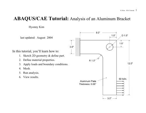
<strong>ABAQUS</strong>/<strong>CAE</strong> <strong>Tutorial</strong>: <strong>Analysis</strong> <strong>of</strong> <strong>an</strong> <strong>Aluminum</strong> <strong>Bracket</strong><br />
Hyonny Kim<br />
last updated: August 2004<br />
In this tutorial, you’ll learn how to:<br />
1. Sketch 2D geometry & define part.<br />
2. Define material properties.<br />
3. Apply loads <strong>an</strong>d boundary conditions.<br />
4. Mesh.<br />
5. Run <strong>an</strong>alysis.<br />
6. View results.
H. Kim – FEA <strong>Tutorial</strong> 2<br />
Helpful Tips Before Getting Started<br />
Use Exceed 9.0 or equivalent PC terminal s<strong>of</strong>tware.<br />
HELP<br />
Online help m<strong>an</strong>uals: abaqus_aae doc & - there is a “book” for <strong>CAE</strong>: “<strong>ABAQUS</strong>/<strong>CAE</strong> User's M<strong>an</strong>ual”. Context<br />
sensitive help is also available within <strong>CAE</strong>.<br />
<strong>CAE</strong> creates the .inp file which you c<strong>an</strong> edit <strong>an</strong>d run by the comm<strong>an</strong>d line, or you c<strong>an</strong> submit jobs from within <strong>CAE</strong>.<br />
Other files are .cae (<strong>CAE</strong> model file), .odb, .dat, .log, .msg, <strong>an</strong>d .sta. The .dat is the text output file that will<br />
contain results. The .odb file is the binary output file that will be read during post-processing to view graphical<br />
results. The .log file keeps a text record <strong>of</strong> all processes <strong>an</strong>d is useful for checking the status <strong>of</strong> the <strong>an</strong>alysis. The<br />
.msg lists the progress <strong>of</strong> the <strong>an</strong>alysis, as well as provides some messages about why <strong>an</strong> <strong>an</strong>alysis might have<br />
crashed (this information is <strong>of</strong>ten within the .dat file as well). The .sta file is a summary <strong>of</strong> the information<br />
contained in the .msg file, <strong>an</strong>d is useful for monitoring the status <strong>of</strong> long-running jobs during their computation.<br />
MOUSE<br />
Use <strong>of</strong> the Mouse:<br />
– button 1 (left) is select, button 2 (right) gives menu, button 3 (middle, if available is “enter” or “done”)<br />
– multiple items c<strong>an</strong> be selected by: “dragging” a window or holding the SHIFT key while picking<br />
– items c<strong>an</strong> be de-selected by holding the CTRL key.
H. Kim – FEA <strong>Tutorial</strong> 3<br />
<strong>ABAQUS</strong>/<strong>CAE</strong>: Getting Started, Create Part<br />
• To run <strong>ABAQUS</strong>/<strong>CAE</strong>, first go<br />
to the directory you wish your<br />
files to be located, then type:<br />
abaqus_aae cae<br />
or<br />
/usr/site/aae/bin/abaqus_aae cae<br />
• click Create Model Database<br />
• In the Module dropdown box,<br />
select Part (this takes about 30<br />
seconds for the program to<br />
initialize)<br />
• Note the locations <strong>of</strong>: Tool Bar,<br />
Menu Bar, Toolbox Area,<br />
Prompt Area. These will be<br />
referred to repeatedly in the<br />
future.<br />
• In the Toolbox Area, click<br />
Create Part button. The Create<br />
Part window will pop up.<br />
• Enter in name, e.g., bracket<br />
• Under Modeling Space, choose<br />
2D Pl<strong>an</strong>ar<br />
• Base Feature, Shell<br />
• Approximate size: 20<br />
• click Continue…
H. Kim – FEA <strong>Tutorial</strong> 4<br />
Sketch Part<br />
• The window will ch<strong>an</strong>ge to that shown at right.<br />
Note the buttons pointed out.<br />
– Buttons with a dark tri<strong>an</strong>gle will provide more<br />
button choices when clicked <strong>an</strong>d held. Try it.<br />
– Float your mouse pointer over buttons, it will<br />
give a pop-up description.<br />
– Context-Sensitive Help is available. Click the<br />
help button, then the item you w<strong>an</strong>t more info on.<br />
1. Click Create Lines button. Note it is<br />
highlighted when active. In prompt area, enter<br />
in the coordinates:<br />
1. 0, 0 <br />
2. 8, 0 (it is ok if point is be out <strong>of</strong> view)<br />
3. 8, -12 <br />
4. 5, -12 <br />
5. 5, -3 <br />
6. 0, -3 <br />
7. click on point 1 (box will appear on it). Finished<br />
product will be yellow outline <strong>of</strong> the bracket.<br />
Click Auto-Fit View button to re-scale image. The<br />
other buttons adjacent to this one will adjust<br />
p<strong>an</strong>ning, rotation, <strong>an</strong>d zoom. Try them out.<br />
Dynamic viewing with mouse buttons by holding<br />
CTRL + ALT on right side <strong>of</strong> keyboard. Try it.<br />
2. Click Create Circle button. Enter 6.5, -1.5 for<br />
center, <strong>an</strong>d 7.25, -1.5 for perimeter point.<br />
3. Click Create Fillet button… (go to next page)
H. Kim – FEA <strong>Tutorial</strong> 5<br />
Sketch Part – contd.<br />
3. cont’d… enter 1.0 for fillet radius in the Prompt Area, hit enter, then Mouse click on inner two lines when prompted.<br />
• The Create Fillet button should still be highlighted. Click this again to get the screen shown below left.<br />
• Click the Done button in the Prompt Area at the bottom <strong>of</strong> the screen.<br />
• You now are returned to the Part Module screen. This should look like the screen below right. Note different tool<br />
buttons shown in the Toolbox Area.
H. Kim – FEA <strong>Tutorial</strong> 6<br />
Partition Edge<br />
• Click the “Partition Edge:<br />
Enter Parameter” button. In<br />
order to get this button, you<br />
need to click <strong>an</strong>d hold over the<br />
line partitioning tools button –<br />
note the small dark tri<strong>an</strong>gle in<br />
the lower right corner<br />
indicates that this is <strong>an</strong><br />
exp<strong>an</strong>ding button.<br />
• You will be prompted to select<br />
<strong>an</strong> edge, select the far righth<strong>an</strong>d<br />
edge <strong>of</strong> the bracket.<br />
• Click Done.<br />
• In the Prompt Area, enter in<br />
value <strong>of</strong> 0.25 for the<br />
Normalized edge parameter.<br />
• Click the Create Partition<br />
button to finish.<br />
• You will see a large dot onefourth<br />
<strong>of</strong> the way up the edge<br />
<strong>of</strong> the bracket. This<br />
partitioned edge will be used<br />
later for applying a uniform<br />
load.
H. Kim – FEA <strong>Tutorial</strong> 7<br />
Saving <strong>an</strong>d Defining Material Properties<br />
• Save your work: in the Menu<br />
Bar, click File, Save As.<br />
– Under Selection, enter a<br />
name at the end <strong>of</strong> the path,<br />
e.g. bracket. Click OK. From<br />
now on, you c<strong>an</strong> just click<br />
the blue floppy disk icon in<br />
the Tool Bar. Save <strong>of</strong>ten!!!<br />
• Ch<strong>an</strong>ge Modules. In the<br />
Module drop-down box<br />
beneath the Tool Bar, select<br />
Property.<br />
1. Click Create Material Button<br />
– enter a name, e.g. <strong>Aluminum</strong>,<br />
select Mech<strong>an</strong>ical --><br />
Elasticity --> Elastic<br />
– enter 10e6 for Young’s<br />
Modulus, 0.3 for Poisson’s<br />
Ratio.<br />
– click OK<br />
If you w<strong>an</strong>t to modify the material,<br />
click the Material M<strong>an</strong>ager button<br />
to the right <strong>of</strong> Create Material,<br />
select the material by name <strong>an</strong>d<br />
click Edit, or click Dismiss to leave<br />
without making <strong>an</strong>y ch<strong>an</strong>ges.
H. Kim – FEA <strong>Tutorial</strong> 8<br />
Assign Properties to Regions <strong>of</strong> Model<br />
2. Click Create Section Button<br />
– enter a name, e.g., plate<br />
– choose Solid <strong>an</strong>d<br />
Homogeneous<br />
– click Continue<br />
– select the material <strong>Aluminum</strong><br />
(or what ever you named it,<br />
there should be only one to<br />
choose from) in the drop down<br />
box<br />
– enter Pl<strong>an</strong>e stress/strain<br />
thickness: 0.05. Click OK.<br />
3. Click Assign Section Button<br />
– you will be prompted to select a<br />
region. Click on the part.<br />
– Click the Done button in the<br />
Prompt Area at the bottom <strong>of</strong><br />
the screen.<br />
– The Assign Section window<br />
will pop up. Select the Section<br />
Name you wish to assign to this<br />
region (there should be only<br />
one which you’ve previously<br />
named, e.g., plate)<br />
– click OK.
H. Kim – FEA <strong>Tutorial</strong> 9<br />
Inst<strong>an</strong>ce Part<br />
• Ch<strong>an</strong>ge Modules. In the<br />
Module drop-down box<br />
beneath the Tool Bar,<br />
select the Assembly.<br />
– note, the C<strong>an</strong>vas<br />
(main working<br />
graphical window)<br />
will be bl<strong>an</strong>k.<br />
• Click the Inst<strong>an</strong>ce Part<br />
button. The Create<br />
Inst<strong>an</strong>ce window will<br />
pop up.<br />
• Select the part you wish<br />
to inst<strong>an</strong>ce, e.g., the part<br />
we named bracket<br />
previously. A red<br />
outline <strong>of</strong> the bracket<br />
will show.<br />
• Click OK.
H. Kim – FEA <strong>Tutorial</strong> 10<br />
Step<br />
• Ch<strong>an</strong>ge Modules. Select the<br />
Step module.<br />
• Click the Create Step button.<br />
– Create Step window pops up<br />
– enter a name – use the<br />
default name Step-1.<br />
– be sure Procedure type is set<br />
to General, <strong>an</strong>d Static,<br />
General is highlighted in the<br />
list. Click Continue.<br />
• Edit Step window pops up,<br />
with the Basic tab active.<br />
– enter in a Description, e.g.,<br />
apply loading<br />
• Click the Incrementation tab.<br />
– under Increment Size, enter<br />
value <strong>of</strong> 0.1 for Initial. Leave<br />
the rest the same. Full load<br />
corresponds to <strong>an</strong> Increment<br />
value <strong>of</strong> 1 (when Time<br />
Period is set to 1 under the<br />
Basic tab). Setting Initial to<br />
0.1 forces <strong>ABAQUS</strong> to start<br />
the <strong>an</strong>alysis by applying 1/10<br />
<strong>of</strong> the full load. This c<strong>an</strong> also<br />
be left to default 1 value <strong>an</strong>d<br />
the s<strong>of</strong>tware will auto-select.<br />
– click OK.
H. Kim – FEA <strong>Tutorial</strong> 11<br />
Load<br />
• Ch<strong>an</strong>ge Modules. Select the Load module.<br />
• Click the Create Load button.<br />
– the Create Load window pops up.<br />
– enter a Name, e.g., Load-1 is the default<br />
name<br />
– be sure Step-1 (or what name you have<br />
given it) is selected in the Step drop down<br />
box.<br />
– be sure Mech<strong>an</strong>ical is selected in Category<br />
– under Type for selected step, choose<br />
Pressure<br />
– click Continue<br />
– Upon prompting to Select surfaces, mousepointer<br />
click on the lower portion <strong>of</strong> the<br />
right edge <strong>of</strong> the bracket, the region we<br />
partitioned previously. It will highlight red.<br />
– click Done.<br />
– in the Edit Load window that pops up, be<br />
sure to have Distribution set to Uniform,<br />
enter value <strong>of</strong> –1000 in Magnitude, <strong>an</strong>d be<br />
sure that (Ramp) is selected under<br />
Amplitude. This is a 1000 psi traction.<br />
– click OK.<br />
– You should get the image shown to the<br />
right. If your arrows are in the wrong<br />
direction, you need to go back <strong>an</strong>d be sure<br />
to specify a negative pressure.
H. Kim – FEA <strong>Tutorial</strong> 12<br />
Boundary Conditions<br />
• Click the Create Boundary Condition<br />
button.<br />
– the Create Boundary Condition<br />
window pops up.<br />
– enter a name, e.g., fixed edge<br />
– under Category, be sure that<br />
Mech<strong>an</strong>ical is selected.<br />
– under Type for selected step, choose<br />
Displacement/Rotation<br />
– click Continue.<br />
– upon prompt to select regions, mousepointer<br />
click on the upper left vertical<br />
edge <strong>of</strong> the bracket. It will highlight<br />
red.<br />
– click Done.<br />
– Edit Boundary Condition window pops<br />
up.<br />
– be sure Uniform is selected in<br />
Distribution.<br />
– check-mark (click) boxes for u1 <strong>an</strong>d<br />
u2, <strong>an</strong>d leave the default values <strong>of</strong> 0.<br />
– click OK.<br />
– You should get the image shown to the<br />
right
H. Kim – FEA <strong>Tutorial</strong> 13<br />
Seed Mesh<br />
• Ch<strong>an</strong>ge Modules. Select the Mesh<br />
module.<br />
• Click the Seed Part Inst<strong>an</strong>ce button.<br />
This is <strong>an</strong> exp<strong>an</strong>dable button. There<br />
are m<strong>an</strong>y other functions within this<br />
button that are useful for controlling<br />
mesh size.<br />
– In the Prompt Area, enter a Global<br />
element size value <strong>of</strong> 0.5.<br />
– Hit enter <strong>an</strong>d you will see circular<br />
symbols indicating nodal locations<br />
along the part edges.<br />
• Click the Assign Element Type<br />
button.<br />
– the Element Type window pops up.<br />
– choose St<strong>an</strong>dard in Element Library<br />
– Pl<strong>an</strong>e Stress in Family<br />
– Linear in Geometric Order<br />
– within the Quad tab, choose Reduced<br />
Integration in Element Controls.<br />
Leave everything else at default values.<br />
– the text in the lower box should<br />
indicate a CPS4R element<br />
identification. This is a 4-node reduced<br />
integration quadrilateral element.<br />
– click OK.
H. Kim – FEA <strong>Tutorial</strong> 14<br />
Mesh<br />
• Click Mesh Part<br />
Inst<strong>an</strong>ce button.<br />
Note this button has<br />
m<strong>an</strong>y other functions<br />
within it (click-hold<br />
mouse button down<br />
on this button) such<br />
as deleting mesh <strong>an</strong>d<br />
meshing regions <strong>of</strong> a<br />
part.<br />
• Click Yes in the<br />
Prompt Area.<br />
• Your mesh should<br />
look like the image<br />
shown to the right.
H. Kim – FEA <strong>Tutorial</strong> 15<br />
Create Job<br />
SAVE YOUR WORK!!!<br />
• Ch<strong>an</strong>ge Modules. Select the Job<br />
module.<br />
• Click Create Job button.<br />
• Enter a name, e.g., bracket<br />
• Click Continue.<br />
• In the Edit Job window that pops<br />
up, enter a Description, e.g.,<br />
bracket <strong>an</strong>alysis<br />
• Check that Full <strong>an</strong>alysis,<br />
Background, <strong>an</strong>d Immediately<br />
are selected.<br />
• Click OK.
H. Kim – FEA <strong>Tutorial</strong> 16<br />
Submit Job<br />
• Click Job M<strong>an</strong>ager button.<br />
• In Job M<strong>an</strong>ger window pops up,<br />
check that your job is selected, then<br />
click Submit.<br />
• To run your model in Unix Server,<br />
click Write Input. It takes few<br />
seconds to write “job name.inp”.<br />
• Then:<br />
1. Save you job<br />
2. Close <strong>ABAQUS</strong>/<strong>CAE</strong><br />
3. Type “abaqus job = job name”<br />
4. Enter↵<br />
5. Then, go to slide 18-Result (b) for<br />
visualizing results<br />
• Under Status, it will read:<br />
1. Sumbitted<br />
2. Running<br />
3. Completed<br />
• Click Results.<br />
• The Visualization module will run<br />
<strong>an</strong>d the part in outline will be<br />
shown. It should look like the<br />
image to the right.<br />
Write<br />
Input
H. Kim – FEA <strong>Tutorial</strong> 17<br />
Results (a) - Visualization<br />
• Click the Plot<br />
Contours<br />
button.<br />
• A colorful plot <strong>of</strong><br />
Von Mises<br />
stresses appears.<br />
• Color control c<strong>an</strong><br />
be adjusted by<br />
clicking the<br />
Contour<br />
Options button<br />
<strong>an</strong>d adjusting<br />
parameters.<br />
• To select the<br />
scalar field<br />
qu<strong>an</strong>tity plotted,<br />
in the Menu Bar,<br />
select Result,<br />
Field Output,<br />
then choose the<br />
stress component<br />
you wish to plot,<br />
e.g., S11, or U1.<br />
• Click OK.<br />
• Strains, Spatial<br />
Displacements,<br />
etc., c<strong>an</strong> be<br />
selected through<br />
Field Output.
H. Kim – FEA <strong>Tutorial</strong> 18<br />
Results (b) - After Run Model on Unix Server<br />
• Run <strong>ABAQUS</strong>/<strong>CAE</strong> or<br />
<strong>ABAQUS</strong>/VIEWER.<br />
• Open “job name.odb”.<br />
• Click the Plot Contours<br />
button.<br />
• A colorful plot <strong>of</strong> Von<br />
Mises stresses appears.<br />
• Color control c<strong>an</strong> be<br />
adjusted by clicking the<br />
Contour Options button<br />
<strong>an</strong>d adjusting parameters.<br />
• To select the scalar field<br />
qu<strong>an</strong>tity plotted, in the<br />
Menu Bar, select Result,<br />
Field Output, then choose<br />
the stress component you<br />
wish to plot, e.g., S11, or<br />
U1.<br />
• Click OK.<br />
• Strains, Spatial<br />
Displacements, etc., c<strong>an</strong> be<br />
selected through Field<br />
Output.