optical
optical optical
Blackbody Radiation An illustration of the setup for the blackbody experiment is shown in Fig. 4, and a photograph is provided in Fig. 5. Fig. 4. Schematic of the blackbody radiation setup Fig. 5. A photograph of the blackbody radiation setup 8
In Fig. 5, the tungsten lamp is inside the enclosure to the left. An adjustable iris just outside the enclosure is used to vary the amount of light falling on the fiber connected to the HR2000+ spectrometer. For estimating the surface area of the filament A, use the photographs of the filament shown in Fig. 6. The dimensions of the filament coil region are 4.06×2.22×1.00 mm, and the filament wire diameter is 0.229 mm. The leads below the coil are 8.0 mm long. Fig. 6. Pictures of the tungsten 12 V, 100 W lamp filament. On the left is the front view and on the right is the side view. 1. Set up the experiment according to the schematic in Fig. 4 and align the optics. 2. Set the tungsten filament at a certain power (make sure the input power and voltage are smaller than 100 W and 12 V), and collect the blackbody spectrum with HR2000+ spectrometer. You may find that the intensity of the light radiated by the filament is so high that the spectrum always saturates even for the minimum integration time. If this happens, change the iris size and/or change the integration time of the spectrometer. Take a background spectrum for subtraction when you analyze the data. 3. Change the input power for the filament and repeat step 2 to get several spectra at different input powers. 4. Using Eq. 1 to fit your spectra, you should be able to determine the temperature of the filament at a certain input power. You will need to account for the absorptivity as a function of both wavelength and temperature (provided in Fig. 3). You will want to fit the data in Fig. 3 in order to come up with an analytical absorptivity function as an approximation. 5. Once you determine the temperature for each power, you can plot the power supplied to the lamp I dc V dc versus T 4 . Using Eq. 2, determine a value for the Stefan-Boltzmann constant. Optical Absorbance by Light Sensitive Molecules and Beer’s Law An illustration of the setup for the absorbance experiment is shown in Fig. 7, and a photo- 9
- Page 1 and 2: OPTICS INTRODUCTION The optics lab
- Page 3 and 4: explanation of the photoelectric ef
- Page 5 and 6: Fig. 3. Absorptivity for tungsten a
- Page 7: Photoluminescence Photoluminescence
- Page 11 and 12: silica for a wavelength range of 20
- Page 13: 1. Set up the experiment according
In Fig. 5, the tungsten lamp is inside the enclosure to the left. An adjustable iris just<br />
outside the enclosure is used to vary the amount of light falling on the fiber connected to<br />
the HR2000+ spectrometer.<br />
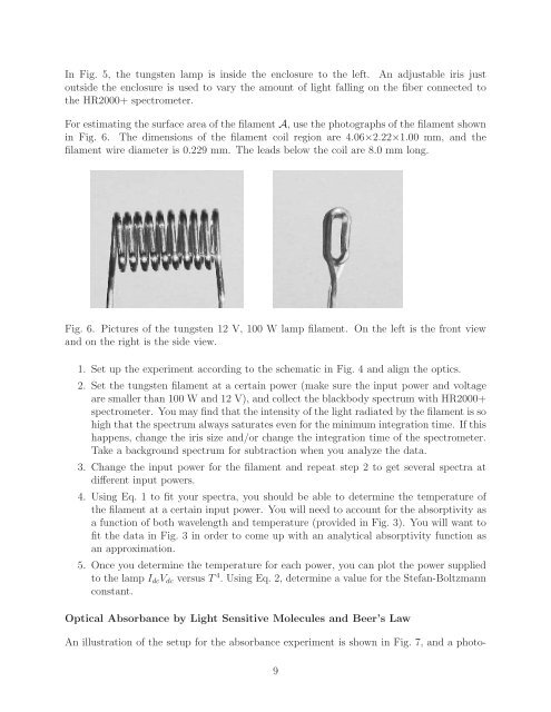
For estimating the surface area of the filament A, use the photographs of the filament shown<br />
in Fig. 6. The dimensions of the filament coil region are 4.06×2.22×1.00 mm, and the<br />
filament wire diameter is 0.229 mm. The leads below the coil are 8.0 mm long.<br />
Fig. 6. Pictures of the tungsten 12 V, 100 W lamp filament. On the left is the front view<br />
and on the right is the side view.<br />
1. Set up the experiment according to the schematic in Fig. 4 and align the optics.<br />
2. Set the tungsten filament at a certain power (make sure the input power and voltage<br />
are smaller than 100 W and 12 V), and collect the blackbody spectrum with HR2000+<br />
spectrometer. You may find that the intensity of the light radiated by the filament is so<br />
high that the spectrum always saturates even for the minimum integration time. If this<br />
happens, change the iris size and/or change the integration time of the spectrometer.<br />
Take a background spectrum for subtraction when you analyze the data.<br />
3. Change the input power for the filament and repeat step 2 to get several spectra at<br />
different input powers.<br />
4. Using Eq. 1 to fit your spectra, you should be able to determine the temperature of<br />
the filament at a certain input power. You will need to account for the absorptivity as<br />
a function of both wavelength and temperature (provided in Fig. 3). You will want to<br />
fit the data in Fig. 3 in order to come up with an analytical absorptivity function as<br />
an approximation.<br />
5. Once you determine the temperature for each power, you can plot the power supplied<br />
to the lamp I dc V dc versus T 4 . Using Eq. 2, determine a value for the Stefan-Boltzmann<br />
constant.<br />
Optical Absorbance by Light Sensitive Molecules and Beer’s Law<br />
An illustration of the setup for the absorbance experiment is shown in Fig. 7, and a photo-<br />
9


