optical
optical
optical

You also want an ePaper? Increase the reach of your titles
YUMPU automatically turns print PDFs into web optimized ePapers that Google loves.
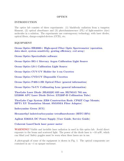
OPTICS<br />
INTRODUCTION<br />
The optics lab consists of three experiments: (1) blackbody radiation from a tungsten<br />
filament, (2) <strong>optical</strong> absorbance and (3) photoluminescence (PL) of light-sensitive (dye)<br />
molecules in a solution. The experiments use contemporary technology, with laser diodes,<br />
<strong>optical</strong> fibers, charge-coupled-devices (CCD), etc.<br />
EQUIPMENT<br />
Ocean Optics HR2000+ High-speed Fiber Optic Spectrometer (operation,<br />
data sheet, system sensitivity, grating efficiency, ccd array)<br />
Ocean Optics SpectraSuite software<br />
Ocean Optics HG-1 Mercury Argon Calibration Light Source<br />
Ocean Optics LS-1 Calibration Light Source<br />
Ocean Optics CUV-UV Holder for 1-cm Cuvettes<br />
Ocean Optics CVD-UV Disposable Cuvettes<br />
Ocean Optics P400-1-SR Optical Fiber (general information)<br />
Ocean Optics 74-UV Collimating Lens (general information)<br />
ThorLabs Laser Diode (HL6322G 635 nm, HL7851G 785 nm,<br />
LD2000 APC Laser Diode Driver, LT220P-B Collimation Tube)<br />
ThorLabs Cage System (ER8 Construction Rods, CP02T Cage Mounts,<br />
HPT1 XY Translation Mount, SM1SMA Fiber Adapter)<br />
Indocyanine Green (ICG)<br />
Hexamethyl indotricarbocyanine tetrafluoroborate (HITC-BF4)<br />
Agilent E3633A DC Power Supply (User Guide, Service Guide)<br />
Coherent LaserCheck laser power meter<br />
WARNING! Visible and invisible laser radiation in used in this optics lab. Avoid direct<br />
exposure to the beam and scattered light. The power of the diode laser is ∼10 mW, which<br />
can blind you! Safety goggles must be worn when these lasers are in use.<br />
A photograph of some of the equipment is shown in Fig. 1. The <strong>optical</strong> components are<br />
contained in an ∼1 m opaque enclosure.<br />
1
Fig. 1. Photograph of some of the equipment used in the optics experiments.<br />
INSTRUMENT CALIBRATION<br />
The Ocean Optics HR2000+ Fiber Optic Spectrometer measures a light intensity distribution<br />
density (light intensity per unit band of wavelength, with units microwatts per square<br />
centimeter per nanometer, µW/cm 2 -nm) as a function of wavelength. Both the wavelength<br />
axis and the light intensity distribution density axis must be calibrated. An Ocean Optics<br />
HG-1 Mercury Argon Calibration Light Source is used for for calibrating the wavelength,<br />
and an Ocean Optics LS-1 Calibration Light Source is used for calibrating the light intensity<br />
distribution density. After using these calibration sources, be sure to turn them off, because<br />
the bulbs have a finite lifetime.<br />
THEORY<br />
The Photon<br />
The photon is the most abused concept in all of science. The truth of the matter may be<br />
seen in a quote from Albert Einstein:<br />
“All these fifty years of conscious brooding have brought me no nearer to the answer to the<br />
question, ‘What are light quanta?’ Nowadays every Tom, Dick and Harry thinks he knows<br />
it, but he is mistaken.” (1954)<br />
Virtually all “modern physics” textbooks and “photon” web sites claim that Einstein and the<br />
photoelectric effect (and other experiments) showed the particle nature of light. However,<br />
the “particle nature of light” and the “photon” were thought up by others after Einstein’s<br />
2
explanation of the photoelectric effect, and Einstein did not care for these concepts. The<br />
truth is that there is absolutely no experiment which requires that light behave like a particle;<br />
it is completely sufficient that charges (including those in “detectors”) behave according to<br />
quantum mechanics. There is the greatly reduced concept that a photon is related to the<br />
quantization of the electromagnetic field. It is a greatly reduced concept because in all<br />
of physics there are only a few phenomena which actually require the quantization of the<br />
electromagnetic field (which remains absolutely not particle-like): 1) spontaneous emission<br />
from atoms, 2) the Lamb shift, 3) the anomolous magnetic moment of the electron, and a few<br />
other more obscure effects. Virtually all experiments in optics can be explained completely<br />
with classical electromagnetic fields, and there is no need for a “photon”. The photon can<br />
be a useful concept in perturbation approximations (as in Feynman diagrams), but Nature<br />
does not have any need for perturbation approximations. If you want to be a practitioner<br />
of rigorous physics, don’t be like Tom, Dick and Harry; if you simply stop using the term<br />
photon, or in very rare cases refer to “the quantized electromagnetic field”, you will be right<br />
every time. [?]<br />
Blackbody Radiation<br />
Blackbody radiation [?,?] is electromagnetic radiation from a particular type of source. In<br />
the laboratory, blackbody radiation is approximated by the radiation from a small hole<br />
entrance to a large cavity. Any radiation entering the hole would reflect off the walls of the<br />
cavity multiple times and would be unlikely to again find the entrance hole and escape; such a<br />
perfect absorbance of light would make the cavity and hole appear to be “black”. Arguments<br />
invoking thermal equilibrium show that the ideal absorbance is independent of wavelength<br />
and shape of the cavity and depends only on the temperature of the cavity walls, and also<br />
shows that the blackbody will emit the same amount of radiation as it absorbs. The escaping<br />
radiation is characterized by an intensity distribution density as a function of wavelength λ<br />
(and parameterized by the temperature T): ε e (λ; T). Because this quantity is a function of<br />
wavelength, it is often referred to as a “spectral” density, or sometimes simply “spectrum”.<br />
Its units are intensity per band of wavelength, conveniently expressed as microwatts per<br />
square centimeter per nanometer, or µW/cm 2 -nm. It is a “density” in that it must be<br />
multiplied by a wavelength bandwidth in order to obtain an actual radiation intensity (in<br />
µW/cm 2 ); thus ε e (λ; T)dλ gives the intensity of the radiation having wavelengths between<br />
λ and λ + dλ. In 1901 Max Planck showed that for an ideal blackbody<br />
ε e (λ; T) = 2πhc2<br />
λ 5 1<br />
e hc/λk BT<br />
− 1<br />
(1)<br />
where h = 6.626×10 −34 J-s is Plank’s constant, c = 3.00×10 8 m/s is the speed of light, and<br />
k B = 1.38×10 −23 J/K is Boltzmann’s constant. Plots of ε e (λ; T) versus λ for several values<br />
of T are shown in Fig. 2.<br />
3
Fig. 2. Blackbody spectral density versus wavelength for several temperatures.<br />
By integrating the spectral density (Eq. 1) over all wavelengths, one obtains the total radiated<br />
intensity (power per unit area) S e (T) at the temperature T :<br />
S e (T) = 2π5 k 4 B<br />
15c 2 h 3T4 = σ B T 4 (2)<br />
where σ B = 2π 5 k 4 B /15c2 h 3 = 5.67×10 −8 W/m 2 -K 4 is the Stefan-Boltzmann constant.<br />
From the plots in Fig. 2, it can be seen that ε e (λ; T) has a maximum at some λ = λ max for<br />
each T. Taking the derivative of Eq. 1 with to respect to λ and setting it equal to zero gives<br />
an equation which can be solved for λ max as a function of T :<br />
This is known as the Wien displacement law.<br />
λ max = ( 2.90 × 10 −3 m-K ) T −1 (3)<br />
Actual thermal radiation devices are not quite ideal, theoretical blackbodies. Real devices do<br />
not have perfect absorbance but reflect some fraction of any incident radiation. The deviation<br />
from perfect absorbance by a particular material is given by a function a e (λ; T) < 1; because<br />
of the balance between absorption and emission of radiation, this quantity is referred to as<br />
either absorptivity or emissivity. For real devices approximating a blackbody, the formulas<br />
for ε e (λ; T) and S e (T) must be multiplied by the absorptivity a e (λ; T) characterizing the<br />
device. In the optics lab experiment on blackbody radiation, the radiator involves a tungsten<br />
filament; the absorptivity function for tungsten is shown in Fig. 3.<br />
4
Fig. 3. Absorptivity for tungsten as a function of wavelength and temperature.<br />
In the derivation of the blackbody formulas, it is assumed that the blackbody is in equilibrium<br />
with (and hence at the same temperature as) its environment. However, in the optics<br />
lab blackbody experiment, the device approximating the blackbody is heated to a temperature<br />
T significantly above its environment, which is at room temperature T 0 ≃ 300 K; thus<br />
the formula for blackbody power radiation must be modified, as will be shown below. Furthermore,<br />
the experimental blackbody will also lose energy due to heat being removed by<br />
convection in the surrounding air; this power loss is linearly proportional to the difference<br />
in the device temperature T and the environment temperature T 0 . The total power lost by<br />
the blackbody device due to being out of thermal equilibrium with its environment must be<br />
supplied by an external source; in the case of the optics lab blackbody device, this is the<br />
electrical power delivered to the tungsten filament. By conservation of energy we have<br />
I dc V dc = κ (T − T 0 ) + 〈a e 〉 (T)σ B A ( )<br />
T 4 − T0<br />
4 (4)<br />
where I dc is the DC current passing through the tungsten filament, V dc is the voltage drop<br />
across the filament, κ is the effective thermal conductivity due to convection in the air,<br />
〈a e 〉 (T) is an average of a e (λ; T) over wavelengths for which data are taken, and A is an<br />
estimate of the area of the tungsten filament.<br />
With the above formulas, the goals of the optics lab blackbody experiment may be outlined<br />
as follows:<br />
(a) By measuring the spectral density of the radiation from the tungsten filament and com-<br />
5
paring with the appropriate formula, the temperature T of the filament may be determined.<br />
By adjusting the electrical power delivered to the filament, different temperatures may be<br />
measured.<br />
(b) Using several values of T, the electrical power I dc V dc may be plotted versus T 4 , and the<br />
slope of a fitted line may be used to determine a value for σ B .<br />
Optical Absorbance by Light Sensitive Molecules and Beer’s Law<br />
The Beer-Lambert Law [?], more commonly known as Beer’s law, states that the <strong>optical</strong><br />
absorbance by a light-sensitive molecule (e.g., a dye molecule) in a transparent solvent varies<br />
linearly with both the sample cell path length and the concentration of the molecules in the<br />
solvent. In practice, Beer’s law is accurate enough for a range of light-sensitive molecules,<br />
solvents and concentrations, and is a widely used relationship in quantitative spectroscopy.<br />
Absorbance is measured in a spectrophotometer by passing a collimated beam of light at<br />
wavelength λ through a plane parallel slab of material that is normal to the beam. For<br />
liquids, the sample is held in a an <strong>optical</strong>ly flat, transparent container called a cuvette.<br />
Optical absorbance OA is calculated from the ratio of the spectral density transmitted<br />
through the sample ε ′ e (λ) to the spectral density that is incident on the sample ε e (λ) (with<br />
T = room temperature).<br />
ε ′ e (λ)<br />
OA = − log 10 (5)<br />
ε e (λ)<br />
For a sample with an <strong>optical</strong> pathlength l and a molar concentration C m [with units of<br />
molarity (M), defined as a mole per liter (mol/L)], Beer’s law can be stated as<br />
OA = α m (λ)lC m (6)<br />
where α m (λ) is the coefficient of molar absorptivity (also known as the extinction coefficient)<br />
of the molecule at wavelength λ. α m (λ) has units M −1 m −1 , and is a property of the material<br />
and the solvent.<br />
In an absorbance experiment, light is attenuated not only by the light-sensitive molecule<br />
but also by reflections from the interface between air and the cuvette, the cuvette and the<br />
sample, and absorbance by the solvent. These factors can be quantified separately, but<br />
are often removed by defining ε e (λ) as the light intensity passing through a sample blank<br />
or reference sample (e.g., a cuvette filled with solvent but with zero concentration of the<br />
light-absorbing molecule).<br />
In the optics lab, the transmitted spectral density ε e ′ (λ) of various samples with different<br />
concentration and the sample blank spectral density ε e (λ) are measured so as to determine<br />
the absorbance OA. By fitting the absorbance OA versus the concentration C m , which should<br />
have linear relation, Beer’s law may be verified. The measurements will be performed on<br />
solutions of two different dye molecules, indocyanine green (ICG) [?] and hexamethylindotricarbocyanine<br />
tetrafluoroborate (HITC-BF4) [?] solutions.<br />
6
Photoluminescence<br />
Photoluminescence (PL) [?] is a process in which a chemical compound absorbs electromagnetic<br />
radiation, makes a transition to a higher electronic energy state, and then re-emits<br />
electromagnetic radiation upon returning to a lower energy state. In stricter terms it is “luminescence<br />
arising from photoexcitation”. The time delay between absorption and emission<br />
is typically extremely short, on the order of 10 nanoseconds. Under special circumstances,<br />
however, this period can be extended into minutes or hours.<br />
In this experiment, the concentration dependence of photoluminescence will be measured for<br />
indocyanine green (ICG) and hexamethylindotricarbocyanine tetrafluoroborate (HITC-BF4)<br />
solutions.<br />
PROCEDURE<br />
Calibration<br />
The HG-1 Mercury Argon Calibration Light Source is used to calibrate the x-axis (wavelength<br />
axis) of the HR2000+ spectrometer. Connect the HG-1 to the HR2000+ with a<br />
fiber optic cable, and take a spectrum with the SpectraSuite software. Fit each peak in the<br />
spectrum with an appropriate function (Gaussian, Lorentzian, or other?) to determine the<br />
wavelength at the peak, λ fit . Make a plot of (λ − λ fit ) versus λ, where the values of λ are<br />
the accepted values of the spectral lines for the HG-1. What is the mean apparent error for<br />
the range of 200 to 1000 nm?<br />
The LS-1 Calibration Light Source is used to calibrate the y-axis (spectral density axis) of<br />
the HR2000+ spectrometer. Make a measurement as with the HG-1, but also make a measurement<br />
with the LS-1 off to obtain a background spectrum; in the data analysis, subtract<br />
the background from the measured LS-1 spectrum. Determine the HR2000+ calibration<br />
curve by comparing the measured LS-1 spectrum with the actual LS-1 spectrum which is<br />
given by a blackbody spectrum at 2000 K, multiplied by an absorptivity curve given by:<br />
where the coefficients are given by<br />
a e (λ) = C 0 + C 1 λ + C 2 λ 2 + C 3 λ 3 + C 4 λ 4 + C 5 λ 5 + C 6 λ 6 (7)<br />
C 0 -1.07983×10 0<br />
C 1 1.58273×10 −2<br />
C 2 -6.41915×10 −5<br />
C 3 1.33611×10 −7<br />
C 4 -1.51662×10 −10<br />
C 5 8.90834×10 −14<br />
-2.12064×10 −17<br />
C 6<br />
The calibration can be used from 400 nm to 900 nm. Check to see if your calculated<br />
calibration is in reasonable agreement with a value predicted using the available <strong>optical</strong> fiber<br />
properties, the HC1 grating efficiency curve, and the properties of the charge-coupled-device<br />
(CCD) used in the HR2000+, which together contribute to an “instrument function”.<br />
7
Blackbody Radiation<br />
An illustration of the setup for the blackbody experiment is shown in Fig. 4, and a photograph<br />
is provided in Fig. 5.<br />
Fig. 4. Schematic of the blackbody radiation setup<br />
Fig. 5. A photograph of the blackbody radiation setup<br />
8
In Fig. 5, the tungsten lamp is inside the enclosure to the left. An adjustable iris just<br />
outside the enclosure is used to vary the amount of light falling on the fiber connected to<br />
the HR2000+ spectrometer.<br />
For estimating the surface area of the filament A, use the photographs of the filament shown<br />
in Fig. 6. The dimensions of the filament coil region are 4.06×2.22×1.00 mm, and the<br />
filament wire diameter is 0.229 mm. The leads below the coil are 8.0 mm long.<br />
Fig. 6. Pictures of the tungsten 12 V, 100 W lamp filament. On the left is the front view<br />
and on the right is the side view.<br />
1. Set up the experiment according to the schematic in Fig. 4 and align the optics.<br />
2. Set the tungsten filament at a certain power (make sure the input power and voltage<br />
are smaller than 100 W and 12 V), and collect the blackbody spectrum with HR2000+<br />
spectrometer. You may find that the intensity of the light radiated by the filament is so<br />
high that the spectrum always saturates even for the minimum integration time. If this<br />
happens, change the iris size and/or change the integration time of the spectrometer.<br />
Take a background spectrum for subtraction when you analyze the data.<br />
3. Change the input power for the filament and repeat step 2 to get several spectra at<br />
different input powers.<br />
4. Using Eq. 1 to fit your spectra, you should be able to determine the temperature of<br />
the filament at a certain input power. You will need to account for the absorptivity as<br />
a function of both wavelength and temperature (provided in Fig. 3). You will want to<br />
fit the data in Fig. 3 in order to come up with an analytical absorptivity function as<br />
an approximation.<br />
5. Once you determine the temperature for each power, you can plot the power supplied<br />
to the lamp I dc V dc versus T 4 . Using Eq. 2, determine a value for the Stefan-Boltzmann<br />
constant.<br />
Optical Absorbance by Light Sensitive Molecules and Beer’s Law<br />
An illustration of the setup for the absorbance experiment is shown in Fig. 7, and a photo-<br />
9
graph is provided in Fig. 8.<br />
Fig. 7. Schematic of the absorbance setup<br />
Fig. 8. A photograph of the absorbance setup<br />
The CUV-UV Holder for 1-cm Cuvettes couples to lamps and spectrometers to create an<br />
absorbance or transmission measurement system. Two 74-UV lenses are mounted across the<br />
cell holder for square 1-cm cuvettes. The base includes channels for connection to a water<br />
bath for temperature regulation, and the unit also accepts filters. The 74-UV lens uses fused<br />
10
silica for a wavelength range of 200 to 2000 nm. When focused for collimation, the beam<br />
divergence is 2 degrees or less, depending on the <strong>optical</strong> fiber diameter.<br />
1. Set up the experiment according to the schematic in Fig. 7. The light source here is<br />
the same tungsten filament used for the blackbody radiation experiment.<br />
2. Align the optics so that sufficient light goes into the fiber.<br />
3. Prepare ICG and HITC-BF4 solutions with various concentrations. You may find that<br />
low concentrations (less than 10 −3 M) are preferable for this experiment. A CVD-UV<br />
Disposable Cuvette should be filled with a sample.<br />
4. Put the cuvette with a solution in the CUV-UV Holder and collect the spectra for both<br />
sample spectral density ε e ′ (λ) (with the solution that you want to measure) and blank<br />
spectral density ε e (λ) (with only solvent as a reference).<br />
5. Determine the <strong>optical</strong> absorbance OA by Eq. 5.<br />
6. Repeat steps 4 and 5 for each of the various concentrations.<br />
7. Using Eq. 6, determine the molar absorptivity of your sample.<br />
In your lab report, you should comment on the <strong>optical</strong> properties of the various components<br />
(the cuvette, the cuvette holder and its lenses, etc.) used in the measurement, and how they<br />
might affect the performance of the apparatus.<br />
Photoluminescence<br />
An illustration of the setup for the photoluminescence (PL) experiment is shown in Fig. 9,<br />
and a photograph is provided in Fig. 10.<br />
Fig. 9. Schematic of the photoluminescence setup<br />
11
Fig. 10. A photograph of the photoluminescence setup<br />
In the photoluminescence experiment,<br />
diode lasers at wavelengths of 635 nm and<br />
785 nm are used. You must follow the<br />
safety procedures for using lasers. The<br />
diode lasers are held in a LT220P-B Collimator<br />
Tube and operated with a LD2000<br />
APC Laser Diode Driver. The driver is<br />
contained in a unit made by the Physics<br />
Department Electronics Shop; a photograph<br />
of a laser diode with collimator,<br />
holder and driver is shown in Fig. 11.<br />
Fig. 11. Photograph of a laser diode with collimator,<br />
holder and locally fabricated driver<br />
unit.<br />
12
1. Set up the experiment according to the schematic in Fig. 9.<br />
2. Put on safety goggles and align the optics carefully. The PL intensity from the solution<br />
can be very weak depending on the quality of your alignment and the concentration<br />
of your solution. Use the special spanner wrench to adjust the lens in the front of the<br />
collimation tube. A cage system is used to align the lenses for collecting the light for<br />
the PL spectra. The <strong>optical</strong> axis of the cage should be perpendicular to the direction<br />
of the incident laser. For this geometry, use the cuvette holder that is designed for a<br />
PL experiment. For 785 nm infrared (IR, which is almost invisible) laser, use the IR<br />
sensitive card to check the laser spot and align the optics. (Note: as a safety measure,<br />
the laser will not be lasing if the laser head is not mounted on the laser holder.)<br />
3. Using appropriate excitation (635 nm and/or 785 nm), record the PL spectra of both<br />
ICG and HITC-BF4 solutions with different concentrations.<br />
Acknowledgement: The original experiment design, lab guide, diagrams and photographs<br />
were prepared by Duming Zhang (c. 2005).<br />
References<br />
[1] M. O. Scully and M. Sargent, Physics Today, March 1972, p 38-47, “The concept of the<br />
photon”<br />
[2] F. Reif, Fundamentals of Statistical and Thermal Physics (McGraw-Hill, New York,<br />
1965), pp. 373-388.<br />
[3] Daryl W. Preston, Eric R. Dietz, The Art of Experimental Physics (John Wiley & Sons,<br />
New York, 1991).<br />
[4] J. D. J. Ingle and S. R. Crouch, Spectrochemical Analysis (Prentice Hall, New Jersey,<br />
1988)<br />
[5] M. L. J. Landsman, G. Kwant, G. A. Mook and W. G. Zijlstra, J. Appl. Physiol.,<br />
40, 575-583 (1976). “Light absorbing properties, stability, and spectral stabilization of<br />
indocyanine green”.<br />
[6] Marvin J. Weber, Handbook of Lasers (CRC Press, Boca Raton, FL, 2001).<br />
[7] Donald A. McQuarrie and John D. Simon, Physical Chemistry, a Molecular Approach<br />
(University Science Books, Sausalito, CA, 1997).<br />
13