Static Electricity (Lab 01)

Goals:
Static Electricity
(Two Studies of Electrostatics)
To become familiar with basic electrostatic phenomena
To learn the charge model and learn to apply it to conductors and insulators
To understand polarization and the attraction between neutral and charged objects
To explore quantitatively how the electric force depends upon the distance between
charged bodies.
Equipment:
Sticky tape (e.g. Scotch brand)
PVC pipe
Glass rod
Wool cloth
Rabbit fur
Coulomb’s Law Apparatus
Software: Microsoft Excel
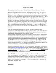
Introduction:
Various civilizations have recorded observations of what we would typically call “static
electricity” for thousands of years, dating back to the ancient Greeks and possibly even earlier.
They noticed that when pieces of amber were rubbed or polished with animal fur, the amber
could attract small bits of straw, even causing them to fly through the air to reach the amber. In
the Elizabethan era, the English physician William Gilbert (1544–1603) first referred to this
attraction as the “electric” attraction, deriving from the Greek word for amber, elektron. From
these early beginnings, we have the modern words of electric, electricity, electrical, and so on.
Gilbert was able to determine two “kinds” of electricity. In his terminology, amber, when rubbed
with fur, acquires “resinous electricity” and when rubbed with silk, acquires “vitreous
electricity.” He noted that pieces of amber with the same kind of electricity repelled each other
and pieces with the opposite kind attracted each other.
Years later, the American printer, author, philosopher, diplomat, inventor and scientist Benjamin
Franklin (1706–1790) proposed that these two “kinds” of electric charge be named positive and
negative, symbolized by (+) and (−), respectively. Franklin claimed that all materials possess a
single kind of electrical “fluid” and that the action of rubbing one material against another did
not create an electrical charge, but merely transferred some of this “fluid” from one body to the
other. He presumed that neutral bodies consisted of equal numbers of positive and negative
charges, and that rubbing transferred some positive charges from one body to another, leaving
the first body with a net negative charged and the other with a net positive charge. He again
confirmed that the same type of charges were found to repel each other while opposite charges
were found to attract each other.

Through a very careful set of experiments involving a torsion balance and equally charged pith
balls, the French engineer Charles Coulomb (1736–1806) was able to quantify the electric
attraction and repulsion in the form we now call “Coulomb’s Law”. Coulomb’s law describes the
force between two charged particles, labeled 1 and 2, and can be stated:
1. If two point particles, having charges q 1 and q 2 respectively, are a distance r apart, the
charges exert forces on each other with a magnitude of:
q1
q2
F
F
k
(Eq. 1)
1on 2
2 on 1
2
r
These forces are equal in magnitude, but opposite in direction
2. The forces are directed along the straight line drawn between the two charges. The forces
are mutually attractive if the charges are opposite, and mutually repulsive for like
charges.
We will not repeat Coulomb’s experiment exactly, but we can make some qualitative
observations using everyday items such as sticky tape, plastic pens, and metal keys, as well as
some quantitative measurements with pith balls. With equipment as simple as this, we can repeat
the same types of experiments that natural philosophers, inventors, and scientists have been
performing for over 2400 years.
Today, the process of rubbing two materials together to transfer some amount of electric charge
is known as tribolectric charging. Table 1 below indicates the relative ability of a material to
gain or lose charges due to rubbing. More plusses (+) next to a material in the chart indicates a
greater ability to obtain a net positive charge. More minuses (−) next to a material in the chart
indicates a greater ability to obtain a net negative charge.
In general when two objects listed in the chart are rubbed together, the material listed higher in
the chart becomes positively charged and the material listed lower in the chart becomes
negatively charged (e.g., when rabbit fur is rubbed on glass, the fur will be positively charged,
the glass negatively). The greater the separation of the materials in the chart, the greater the
magnitude of the charge transferred.
Material Relative charging with rubbing
rabbit fur + + + + + +
glass + + + + +
human hair + + + +
nylon/wool + + +
silk + +
paper +
cotton
−
wood
− −
amber
− − −
rubber
− − − −
PVC
− − − − −
Teflon
− − − − − −
Table 1 Tribolectric charging

We can also characterize how easily charge can flow along or through a material. Materials that
easily allow charge to flow through them are known as conductors. Materials through which
charge cannot easily flow are known as insulators. We understand this distinction today in terms
of the mobility of charge carriers within the material. For instance, in most metals (which are
often good conductors), valence electrons are free to move anywhere throughout the metal, and
thus can easily transfer charge from one location to another within the metal. In insulating
materials, on the other hand, there are relatively few free charge carriers, and so excess charge
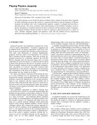
tends to stay where it’s put on the surface of an insulator. At an atomic level, though, we can still
envision a process by which the electrons orbiting their nuclei in an insulator can shift somewhat
to the side due to external influences, a process known as polarization, and depicted in Figure 1.
In the first portion of today’s experiment, you will explore the qualitative aspects of the
electrostatic interaction between insulators, conductors, and differently charged objects.
(a)
(b)
Figure 1 Depiction of polarization of an atom. In (a), a neutral atom is shown with dense, positively charged
nucleus and a negatively charged electron “cloud” (depicted by the shading). In (b), when other charges are nearby,
the electron cloud distorts due to electrostatic forces, and we say that the atom has become polarized (or
equivalently, we say that a dipole moment has been induced). The distortion is greatly exaggerated here.
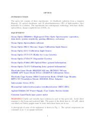
In the second portion of today’s experiment, we will use the apparatus provided to verify
quantitatively the inverse-square law dependence of Coulomb’s Law (Eq. 1). The general setup
of this apparatus is depicted in Figure 2 below. A pith ball with a conductive coating is suspended
by very light strings inside an enclosure which helps to limit the effects of stray air currents. In
this portion of the experiment, you will charge both pith balls with the same type of charge, and
hence they should repel each other. When both balls are at rest, we know that the system is in
equilibrium, and so we can apply our knowledge of Newton’s 1 st Law and the geometry of the
situation to help us relate the positions of the balls and the forces between them.
Based on the free-body diagram presented for you in Figure 2, we can determine the net force in
the x- and y-directions. When the system is in equilibrium, the net force in any direction should
be zero. So, we can write:
F 0 F T sin
Rearranging this, we find:
F
x net
y net
e
0 T cos mg
T sin
mg T cos
If we divide the upper equation by the lower, we find:
F e
F e
tan
mg

T cos θ
T
T sin θ
θ
θ
L
F e
x 1
r
x 2
mg
Figure 2 Schematic of Coulomb’s Law apparatus and associated free-body diagram for hanging mass.
Finally, for the small angles which we will be dealing with in this experiment, we can use the
small-angle approximation tan θ ≈ sin θ. From Figure 2, we can see that sin x
2
/ L . Thus,
solving for the electric force F e , we find
mg
F e
x 2
. (Eq. 2)
L
If we could accurately measure the mass of the suspended ball, and the length of the string
supporting it (and knowing the acceleration due to gravity at the surface of the earth, g), we
could determine the electrostatic force F e by measuring the horizontal displacement of the
suspended ball, x 2 . For our purposes, it will be sufficient to simply note that the electrostatic
force is directly proportional to this horizontal displacement. According to Coulomb’s Law
(Eq. 1) and the relationship we derived in Eq. 2, we can see:
1
F e
or
2
r
. (Eq. 3)
1
x2
2
( x2
x1
)
The verification of this relationship will be our goal in Activity 2 of this lab.

Name: _Solutions___________________
Name: ____________________________
Name: ____________________________
Date: ______________
Lab Sect.: __________
Lab Instructor: ______________________
Directions:
Note: If you are not careful while handling the materials in the activity, you may obtain
inconsistent results. Please follow the directions as faithfully as possible! Also, do not throw out
empty tape dispensers; we can refill them so other students can use them.
Activity 1: Exploring static electricity qualitatively with sticky tape
The following experiments will need you to use strips of tape that are about 20 cm long. Each
time you are asked to use a strip of tape, fold over one end to form a non-sticky handle for easy
handling, as in Figure 3.
Figure 3 Preparing a strip of tape by making a non-stick handle
Stick a 20-cm strip of tape on the lab table, sticky side down. This tape forms a standard base or
“B-strip.” Stick another strip of tape on top of this one, smoothing it down well with your thumb
and fingers. Using a pen or marker, label the handle of this strip with a “T” (for “Top” – this strip
is referred to as a T-strip for the remainder of the lab). With a quick motion, peel off the T-strip
from the base strip. Test whether this T-strip is attracted to your finger – if it is not, remake the
tape. Once you know how to make a T-strip, prepare two such strips.
Holding each one by the handle, bring the slick (non-sticky) sides of the two strips toward each
other. Observe what happens, noting how the behavior changes with the distance between the
strips.
Q1. Describe and explain what happens as the two T-strips are brought closer together.
The T-strips repel as they are brought close together
Q2. What qualitative conclusions can you draw about the relationship between electric force
and the distance between charges? How do your observations relate to Coulomb’s Law?
The closer they are brought together the more strongly they repel. This makes sense since C’s
Law says the force they feel should go like 1/r 2

Q3. Can you tell from your experiment so far whether the T-strips carry a positive charge or a
negative charge? Briefly explain your answer.
We can’t tell whether they are positive or negative from this experiment, merely that they have
the same sign of charge.
Q4. Using the additional equipment that has been supplied to you (the PVC pipe, glass rod, wool
cloth, and rabbit fur) and the information in Table 1, design and carry out an experiment that
allows you to determine the sign of the charge on the T-strips. Describe your experiment and its
results.
If we rub PVC with rabbit fur then the PVC will become negatively charged. We can then test
to see if the T-strips are attracted or repelled by the PVC. If they are attracted then they are
positively charged; if repelled they are negative.
Conclusion: T-tape is attracted to the PVC so positive
Examining a “B” strip
Place another base strip on the lab table as before. This time, use a marker or pen to label the
handle “B” (for "Bottom"). Press another strip of tape on top of the B-strip, sticky side down;
label the handle “T”. Make sure the two strips have stuck to each other smoothly. Now, remove
the pair of strips from the table. Check whether the pair of strips is attracted to your finger – if
you do see an attraction, have one of your teammates rub the slick side of the tape with their
fingers or thumb. This is important: by rubbing your finger along the pair, you discharge the
pair, ensuring that the pair of tape strips is neutral.
Once you have made certain the pair of strips is neutral, peel the pair apart to get a separate T-
strip and B-strip. Let someone else in your team make another pair of B and T strips in the same
manner. As before, your aim is to study the interaction between these different strips by bringing
the slick sides towards each other.

Q5. Summarize the interactions between two T-strips, between two B-strips and between a T-
strip and a B-strip.
T-T interaction: (a) no interaction (b) they attract (c) they repel
B-B interaction: (a) no interaction (b) they attract (c) they repel
T-B interaction: (a) no interaction (b) they attract (c) they repel
Q6. In Q4, you determined the sign of charge on the T-strip. Based on that sign, and the
interactions above, what is the sign of the B-strip? Describe how you could use the same method
you described in Q4 to verify the sign of the B-strip, and do so.
It seems likely that B is negatively charged (opposite sign of T). It isn’t neutral because it repels
the other B.
We can try to confirm by seeing if it is repelled by the negatively charged PVC
Q7. Given that you made certain that the pair of tape strips was neutral before separating the
strips, is it possible to create a T-strip and B-strip that repel each other? Explain why or why not.
No. To repel they must have the same sign of charge, which would require a net charge.

Testing charged strips with conductors and insulators
Make another pair of T and B strips. Suspend them from the edge of the table as shown in Figure
4 below.
T
B
Figure 4 Hanging T-strip and B-strip from edge of table
Hold a conductor (e.g. a metallic object such as a key) near each tape and observe what happens.
(Make sure that you do not allow the conductor to touch the tape.)
Q8. Describe the interaction between the conductor and each strip.
Conductor/T-strip interaction: (a) no interaction (b) they attract (c) they repel
Conductor/B-strip interaction: (a) no interaction (b) they attract (c) they repel
Q9. Using a few sentences and a clear sketch, explain these observations. Your sketch should
show how the different charges in the conductor (i.e., electrons & protons) are distributed when
the conductor is far away from a charged tape strip and when it is close to a charged tape strip.
The charges in the conductor are free to redistribute. When the positively charged T-strip
is brought near the neutral conductor, the conductor polarizes and then attracts the T-strip.
Sketch:

Now, hold an insulator (e.g. the end of a plastic pen or the glass rod, provided that it has been
discharged) near each tape and observe what happens. (Make sure that you do not allow the
insulator to touch the tape.)
Q10. Describe the interaction between the insulator and each strip.
Insulator/T-strip interaction: (a) no interaction (b) they attract (c) they repel
Insulator/B-strip interaction: (a) no interaction (b) they attract (c) they repel
Q11. Using a few sentences and a clear sketch, explain these observations. Your sketch should
show how the different charges in the insulator (i.e., electrons & protons) are distributed when
the insulator is far away from a charged tape strip and when it is close to a charged tape strip.
Though the electrons aren’t free to move in the insulator they are still free to shift, enabling a
weak (compared to the conductor) polarization in the insulator
Sketch:
Q12. Based on your observations, which was stronger: the interaction between the conductor and
the tape strips or the interaction between the insulator and the tape strips? Explain this
observation.
It was hard to see, but the conductor should more strongly attract the tape than the insulator

Activity 2: A quantitative study of Coulomb’s Law
Now, we will set aside the sticky tape and turn our attention to the
Coulomb’s Law apparatus. Our goal with this device is again to
confirm that the electrostatic force between two charged bodies is
inversely proportional to the square of the distance between them.
For ease of calculation, we will adopt a horizontal coordinate
system in which the original, undisturbed equilibrium position of the
hanging ball is used as our origin. (See Figure 2 again for the
geometry involved and Figure 5 for a depiction of our x-coordinate
system.) Again, we will label the horizontal position of the blockmounted
ball with respect to this origin as x 1 , and the horizontal
position of the suspended ball as x 2 . It will not be easy to measure
either x 1 or x 2 directly, but we can relate easy-to-make
measurements to the ones we want.
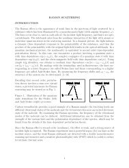
To begin, we will measure the position of the block-mounted ball by measuring the position of
one end of the block itself. (Note: in the explanation which follows, it is assumed that you will be
moving the block on the left-hand side of the apparatus.)
d
block
X
−x
0
+x
block
X 0
Figure 5 Finding the block’s position when the block-mounted ball is just touching the suspended ball.
1. Measure the diameter d of the block-mounted pith ball and record it below:
Diameter of pith balls (d): _1.25 cm________________
2. Touch both pith balls (the block-mounted ball and the suspended one) with your finger to
ensure that both are neutral.
3. Slide the block in its groove into the apparatus, so that the block-mounted ball just barely
comes into contact with the suspended ball without displacing it (see Figure 5).

lock
When the block is at this position (which we will call X
0
), we know that the block-mounted
ball will be at position x 1 = −d (i.e., its center of mass will be one ball-diameter away from the
center of mass of the suspended ball).
4. With the block-mounted ball just barely touching the suspended ball, record the position of
the block:
“Zero” position of the block (
block
X
0
): ___________________________
If we move the block farther to the left, the block-mounted ball’s position with respect to our
origin will become more negative. If we move the block farther to the right, the ball’s position
will become more positive. Using these notions, we can write down an expression for the blockmounted
ball’s center-of-mass position (x 1 ) as a function of the block’s position measured via the
block
measuring tape ( X ) as
block block
x (
X X ) . (Eq. 4)
1 0
d
You should verify for yourself that this expression satisfies the conditions we just described. To
summarize: we will record the block-mounted ball’s position by measuring the position of the
block itself via the measuring tape provided on the outside of the apparatus.
How do we determine the suspended ball’s position? At the back of the Coulomb’s law
apparatus, a separate ruler is mounted below a mirror. If you try to line up the ball with the ruler
at the back of the apparatus, you’ll notice that you can get drastically different position readings
if you move your head left or right. This phenomenon is called parallax, and occurs anytime you
try to compare the transverse positions of objects located different distances away from you. To
help minimize the effect of the parallax, we can try to line up the edge of the ball directly with its
reflection in the mirror. When we do this, we’re looking dead-on at the edge of the ball, and can
trust our reading from the ruler at the back of the apparatus.
So, to find the position of the suspended ball at any point in time, we just line up the edge of the
ball with its reflection in the mirror, and look to see where this lines up with the ruler. This
mirror
position we can call X . When the ball is hanging straight down, we’ll say that its edge is at
mirror
position X
0
(which corresponds to the center of mass being at a position of x 2 = 0). From
these considerations then, we find that the suspended sphere’s center-of-mass position (x 2 ) can be
determined from the measurement with respect to the ruler at the back of the apparatus by
mirror mirror
x X . (Eq. 5)
2
X
0
5. Record the “zero” position of the edge of the suspended ball when it hangs vertically
downward, as measured with the no-parallax method described above with respect to the
ruler in the back of the apparatus.
“Zero” position of edge of the suspended ball (
mirror
X
0
): ___________________________

To facilitate the analysis of the data, and to acclimatize you to using common software tools for
this task, we have provided a spreadsheet with the necessary calculations (e.g. Eqs. 4 and 5)
already provided. Take this opportunity to open the “Static_Electricity.xls” spreadsheet and enter
block
mirror
your measurements for d, X
0
, and X
0
in the spaces provided. Thoroughly read the
directions below on how to perform the experiment (Steps 6 through 11), and then collect your
data in the Excel spreadsheet.
6. Rub your PVC pipe vigorously with the rabbit fur provided to charge the pipe.
7. Charge the block-mounted ball by induction. To do so, first move the block and ball away
from the Coulomb’s Law apparatus. Bring the charged PVC pipe near, but not touching the
block-mounted ball, to within a few centimeters distance. Touch the block-mounted ball with
your finger. Remove your finger from the ball and then remove the PVC pipe from the
vicinity of the ball. The block-mounted ball has now been charged by induction.
8. Slide the block and ball back into the groove in the Coulomb’s Law apparatus (being careful
to not let the ball come into contact with any surface.)
9. Slowly move the block-mounted ball into the apparatus until you see the suspended ball
swing toward it, touch it, and then rapidly swing away. At this point, both the block-mounted
ball and the suspended ball are charged. Move the block-mounted ball 0.5 cm back away
from this position.
10. Slide the block farther into the apparatus as far as you can (but not so far as to push the
block-mounted ball into the suspended ball again; they should still be separated by some
distance.)
11. Humidity in the air and stray air currents will gradually discharge your spheres, so it best to
work quickly. Using the Excel spreadsheet provided, record the positions of the block and the
suspended ball as you slide the block in 2- or 3-mm increments back out of the apparatus.
Take at least 10 or so readings.
Once you have collected your data, proceed with the analysis by answering the following
questions and providing graphs of your data where requested.

Q13. In step 7 of the procedure, you charged the block-mounted ball by induction. Sketch the
distribution of charges (i.e. protons and electrons) on the pith ball, your finger, and the PVC pipe
when (a) you’ve just brought the PVC pipe near the ball, (b), you’ve just touched your finger to
the ball, (c) you remove your finger, and (d) when you move the PVC pipe away from the ball.
(a) PVC brought near to ball
(b) Finger touches ball
(c) Finger moves away from ball
(b) PVC moved away from ball
Q14. In step 9 of the procedure, you charged the suspended ball by conduction. Sketch the net
distribution of charges (i.e. protons and electrons) on both balls, shortly before they touch, at the
moment they touch, and after the suspended ball has swung away.
(a) Block-mounted ball attracts suspended ball
(b) Both balls touch
(c) Suspended ball has swung away

12. You should now attempt to verify (Eq. 3) (the statement that the electrostatic force between
two charged point particles is inversely proportional to the square of the distance between the
charges). To do so, create a plot of the force versus distance (F e vs. r). Include a copy of this
plot in your lab report.
Q15. Does your plot of force versus distance support the statement that the electrostatic force is
inversely proportional to the square of the distance between the charges? Can you quantify to
what extent the data fits or fails to fit this model?
13. We now wish to “linearize” our data by plotting the force versus the inverse of the distance
squared (F e vs. 1/r 2 ). In your Excel file, create a new column of 1/r 2 . Create a plot of force
versus the inverse of the distance squared, and add a linear trendline in order to quantify the
extent to which your data fits the prescribed model (Eq. 3). Include a copy of this plot in your
lab report.
Q16. Is it easier to confirm or deny the relationship described in Eq. 3 via this plot than it was
with the plot of F e vs. r? Why?