L'anguille européenne, indicateurs d'abondance et de ... - ifremer
L'anguille européenne, indicateurs d'abondance et de ... - ifremer
L'anguille européenne, indicateurs d'abondance et de ... - ifremer

Create successful ePaper yourself
Turn your PDF publications into a flip-book with our unique Google optimized e-Paper software.
L’anguille européenne (Anguilla anguilla) est une espèce menacée.<br />
Pendant trois ans, les principaux acteurs concernés par c<strong>et</strong>te situation<br />
– pêcheurs, chercheurs, institutionnels <strong>et</strong> financiers – ont mis en commun<br />
leurs expériences, leurs savoirs institutionnels <strong>et</strong> vernaculaires <strong>et</strong> les ont<br />
adaptés au contexte du réseau <strong>de</strong> bassins versants. C<strong>et</strong> ouvrage fait<br />
la synthèse du proj<strong>et</strong> lancé par l’Ifremer <strong>et</strong> intitulé « InterregIII Espace<br />
Atlantique Indicang » .<br />
Ce gui<strong>de</strong> méthodologique précise la biologie générale <strong>de</strong> l’espèce <strong>et</strong> m<strong>et</strong><br />
en lumière <strong>de</strong>s caractéristiques physiologiques, comportementales,<br />
populationnelles <strong>et</strong> écologiques qui ai<strong>de</strong>ront les gestionnaires à mieux<br />
évaluer son abondance, la nature <strong>de</strong>s modifications que son<br />
environnement naturel a subi ces <strong>de</strong>rnières décennies <strong>et</strong> les pressions<br />
exercées par l’homme sur un bassin versant déterminé. Il définit<br />
<strong>de</strong>s <strong>de</strong>scripteurs, puis <strong>de</strong>s <strong>indicateurs</strong> pour chaque sta<strong>de</strong> du cycle<br />
biologique : civelle, anguille jaune <strong>et</strong> argentée. La partie concernant<br />
l’environnement est fortement développée compte-tenu <strong>de</strong> l’importance<br />
<strong>de</strong> la qualité <strong>de</strong>s milieux dans la reconstitution <strong>de</strong>s stocks d’anguille.<br />
Dès 2009, la réglementation européenne sur l’anguille prévoit <strong>de</strong> m<strong>et</strong>tre<br />
en œuvre <strong>de</strong>s plans <strong>de</strong> gestion <strong>et</strong> <strong>de</strong> restauration <strong>de</strong> c<strong>et</strong>te espèce.<br />
Ce gui<strong>de</strong> perm<strong>et</strong>tra <strong>de</strong> disposer d’une base pratique <strong>et</strong> théorique pour<br />
installer <strong>et</strong>, au besoin, faire évoluer les <strong>indicateurs</strong> nécessaires à l’évaluation<br />
<strong>de</strong> l’efficacité <strong>de</strong> ces plans.<br />
Il intéressera un public averti, les naturalistes <strong>et</strong> les gestionnaires soucieux<br />
<strong>de</strong> la préservation <strong>de</strong> c<strong>et</strong>te espèce. En rappelant les principales notions<br />
sur la dynamique <strong>de</strong>s populations, il sera également un support didactique<br />
pour l’enseignement universitaire.<br />
Les coordinateurs sont <strong>de</strong>s spécialistes reconnus <strong>de</strong> l’anguille européenne.<br />
Patrick Prouz<strong>et</strong>, coordinateur du proj<strong>et</strong> Indicang est directeur <strong>de</strong> programme<br />
à l’Ifremer. Gilles Adam, animateur du comité <strong>de</strong> communication du proj<strong>et</strong>,<br />
est hydrobiologiste <strong>et</strong> chargé <strong>de</strong> mission à la direction régionale <strong>de</strong> l’environnement<br />
Aquitaine. Éric Feunteun, responsable du comité scientifique <strong>et</strong> technique du proj<strong>et</strong>,<br />
est professeur d’ichtyologie <strong>et</strong> d’écologie marine au Muséum national d’histoire<br />
naturelle. Christian Rigaud, co-animateur <strong>de</strong> la thématique « anguille jaune » du proj<strong>et</strong><br />
est ingénieur <strong>de</strong> recherche au Cemagref <strong>et</strong> animateur du groupement d’intérêt<br />
scientifique sur les espèces amphihalines (Grisam).<br />
faire<br />
Savoir<br />
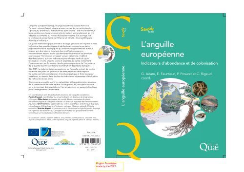
<strong>L'anguille</strong> européenne<br />
Savoir<br />
faire<br />
L’anguille<br />
européenne<br />
Indicateurs d’abondance <strong>et</strong> <strong>de</strong> colonisation<br />
G. Adam, É. Feunteun, P. Prouz<strong>et</strong> <strong>et</strong> C. Rigaud,<br />
coord.<br />
En couverture : L’arbre à anguilles (<strong>de</strong>ssin S. Gros, Ifremer) ; civelle (photo G. Choubert, Inra) ;<br />
anguille jaune (photo G. Adam, Diren Aquitaine) ; anguille argentée (photo H. Farrugio, Ifremer).<br />
Prix : 55 €<br />
Éditions Cemagref, Cirad, Ifremer, Inra<br />
www.quae.com<br />
ISBN 978-2-7592-0085-6<br />
-:HSMHPJ=WUU]Z[:<br />
ISSN : 1952-1251<br />
Réf. : 02091
General introduction<br />
1
Background to the general objectives of the InterregIIIB “Atlantic area”<br />
INDICANG project<br />
Initiated within the framework of the INTERREGIIIB - Atlantic area programme, the INDICANG<br />
project fe<strong>de</strong>rated 40 partners from 4 Atlantic Arc countries 1 . The objective of the project was to<br />
<strong>de</strong>velop and disseminate knowledge concerning the exploitation, habitat and evolution of the<br />
European eel in or<strong>de</strong>r to restore eel stocks which are currently at risk.<br />
The river basin is the relevant scale for the management of the European eel. This scale allows<br />
eel production to be optimized by limiting the constraints related to various anthropogenic factors (one<br />
of which is fishing). Furthermore, it allows commercial fishermen to be fully involved in the project: by<br />
integrating their observations (the commercial fishermen is, in this context, a practitioner who also<br />
un<strong>de</strong>rtakes environmental monitoring) and by involving them in the comparison of the results obtained<br />
from scientific and technical monitoring with those from the monitoring of exploitation indicators (total<br />
catches, fishing effort, catch per unit of effort, climatic variability….). The scale of the river basin also<br />
makes it possible to un<strong>de</strong>rtake a systemic type of analysis.<br />
Eel population abundance and habitat quality were therefore assessed in 13 river basins (figure<br />
1). The principal disturbance factors were i<strong>de</strong>ntified.<br />
From these observations and their comparison, the project partners have <strong>de</strong>fined relevant and<br />
inexpensive indicators relating to the quality of the environment, the abundance of elvers migrating up<br />
the estuaries, the intensity of upstream colonisation by young eels and the abundance of silver eels<br />
migrating towards the Sargasso sea.<br />
The project does not fulfil explicitly the request from the European Union concerning the state of<br />
the population and the level of escapement in relation to the <strong>de</strong>fined reference targ<strong>et</strong> i.e. “40% of<br />
silver eel biomass produced in a pristine environment” because those involved in the project do not<br />
currently have the elements to provi<strong>de</strong> an accurate answer.<br />
The project partners emphasised the need to implement tools and m<strong>et</strong>hodologies that would<br />
enable managers to assess and compare the efficacy of species restoration plans which have to be<br />
<strong>de</strong>fined and implemented from the 1st of January 2009 2 .<br />
1<br />
EU Community Programme > 2000 – 2006, annex 1 of the Indicang Report,<br />
http://www.<strong>ifremer</strong>.fr/indicang.<br />
2<br />
Article (CE) No 1100/2007 of the Council of 18 September 2007, Official Journal of the European Union, annex 2 of the<br />
Indicang report, http://<strong>ifremer</strong>.fr/indicang<br />
2
Tamar, Camel<br />
and Slapton Ley<br />
La Vilaine<br />
La Loire <strong>et</strong> la<br />
Sèvre Niortaise<br />
Minho<br />
L’Adour<br />
La Giron<strong>de</strong>, Garonne<br />
Dordogne<br />
Nalon<br />
Esva<br />
L’Oria<br />
Figure 1 -<br />
Geographical location of river basins covered by the INDICANG project.<br />
Some preliminary <strong>de</strong>finitions to clarify the objectives of the handbook<br />
The notions of <strong>de</strong>scriptor and indicator are <strong>de</strong>fined in the newsl<strong>et</strong>ter number 2 of the<br />
INDICANG project 3 . Once an object is <strong>de</strong>scribed according to various criteria, its state can then be<br />
assessed using these two elements in comparison with various reference frameworks.<br />
• Indicator: Analytical information summarizing the state of a system or its evolution in relation to<br />
specific objectives. This second aspect is most notably used in ISO standard 8042.<br />
• Descriptor: Qualitative or quantitative element, observed, measured or calculated, used to<br />
<strong>de</strong>scribe an object, an individual or a system. For example, the taxonomy of the eel entity uses the<br />
following <strong>de</strong>scriptors: the class (Osteichthyes); the or<strong>de</strong>r (Anguilliforms); the family (Anguillidae);<br />
the genus (Anguilla); the species (anguilla) and a vernacular name (European eel).<br />
• Criteria: Element or information allowing a judgment or a choice to be ma<strong>de</strong> concerning an<br />
object, an individual or a system. It implies the existence of a norm against which to evaluate and<br />
judge.<br />
3<br />
Indicang newsl<strong>et</strong>ter, 2/2006, 3, annex 3 of the Indicang report, http://www.<strong>ifremer</strong>.fr/indicang.<br />
3
A good indicator must:<br />
be relevant and reliable<br />
be sensitive<br />
be synoptic<br />
be shared and interpr<strong>et</strong>able<br />
be available over a significant period<br />
of time<br />
validated scientifically and statistically<br />
reveals the evolution being monitored<br />
summarises complex phenomena, it generally<br />
results from the combination of several<br />
<strong>de</strong>scriptors.<br />
including by non-specialists where it aids<br />
management<br />
takes into account the notion of technical and<br />
economic feasibility<br />
It is useful to collate these different indicators and their associated reference frameworks into<br />
tools, usually called “Management charts”, which offer a synoptic view of the system un<strong>de</strong>r study as a<br />
function of a certain number of evaluation criteria 4 .<br />
The project partners consi<strong>de</strong>red that there was a minimal management chart as opposed to<br />
an optimal management chart.<br />
At a workshop held in Porto in 2006, it was agreed that a minimal management chart must<br />
inclu<strong>de</strong> indicators concerning the importance of available production areas taking into account the<br />
difficulty of access to yellow and silver eel production sites and indicators of 2 types of anthropogenic<br />
mortality: fishing and hydroelectric production. Anything less than this means that the eel production<br />
capacity of the hydrographic system cannot be evaluated.<br />
The optimal management chart is <strong>de</strong>fined by the inclusion of all the indicators <strong>de</strong>scribed in this<br />
handbook. However, an improved management chart can be established by adding to the minimal<br />
management chart some <strong>de</strong>scriptors concerning the chemical quality of the aquatic environment and<br />
the health status of the individuals observed or caught 5 .<br />
Finally, the main technical terms used in this handbook and more broadly within the INDICANG<br />
project framework are <strong>de</strong>fined in the project glossary 6 .<br />
4<br />
For an illustration, please refer to the web site of the > http://www.anguille-loire.com.<br />
5 Girard P., Elie P., 2007. Manuel d’i<strong>de</strong>ntification <strong>de</strong>s principales lésions anatomo-morphologiques <strong>et</strong> <strong>de</strong>s principaux parasites<br />
externes <strong>de</strong>s anguilles, Cemagref, report 110, annex 4 of the Indicang report, http://www.<strong>ifremer</strong>.fr/indicang.<br />
6<br />
Collective, 2007. Glossaire Indicang – Langue francaise, annex 5 of the Indicang report, http://www.<strong>ifremer</strong>.fr/indicang.<br />
4
Handbook contents and instructions<br />
The biological objective of the European regulation relating to eel management 7 is to improve<br />
very significantly the global flux of potential spawners leaving their growth area to r<strong>et</strong>urn to their<br />
reproductive area. This global flux inclu<strong>de</strong>s the production from all river basins and coastal zones<br />
colonised by the species. First it must be noted that the Indicang programme only took into account<br />
inland areas (from the salt-water estuary to the upper reaches of rivers) and consequently so does this<br />
handbook. This increased flux, which will inevitably be progressive, requires in particular a marked<br />
increase in the survival rate from the glass eel stage, in all lower reaches of river basins, to the silver<br />
eel stage over the compl<strong>et</strong>e distribution area of the species.<br />
Starting from a very poor situation, monitoring via relative indices could show abundance<br />
r<strong>et</strong>urning to 1970s-1980s levels, at least in a first intermediate phase. These types of monitoring could<br />
also concern anthropogenic pressures exerted more or less directly on the species. Quantified<br />
objectives of flux, stock and/or survival are also proposed based on the correlation b<strong>et</strong>ween the<br />
<strong>de</strong>gree of colonisation at the entrance to a river basin (and more particularly to the estuary) and the<br />
minimal resulting yield of spawners a few years later. Of course, these two complementary<br />
approaches correspond to different estimation m<strong>et</strong>hods including in terms of cost and time. Within this<br />
handbook, the review of currently available m<strong>et</strong>hodologies specifies the type of approach relating to<br />
different m<strong>et</strong>hods.<br />
Within a river basin, total spawner production inclu<strong>de</strong>s that of tidal compartments (accessible<br />
without having to pass any barriers and without having to swim against the current) and that of<br />
upstream non-tidal compartments. Here also, the m<strong>et</strong>hodological review takes into account the<br />
existence of these compartments and the impact of their characteristics on the monitoring procedures<br />
that have to be implemented.<br />
Finally, within the framework of a local eel management plan at the scale of the river basin,<br />
two supplementary analyses are fully justified in these compartments:<br />
• I<strong>de</strong>ntify the species local characteristics - mainly the distribution and the abundance levels by<br />
sex, age or size class; but also the health condition and the reproductive quality of produced<br />
spawners;<br />
• I<strong>de</strong>ntify human pressures, their localisation, their intensity and the magnitu<strong>de</strong> of their impact on<br />
global survival b<strong>et</strong>ween glass eels entering the system and silver eels r<strong>et</strong>urning to the sea and on<br />
the quality of individuals which are to migrate to the Sargasso sea;<br />
For each of these approaches, the actions un<strong>de</strong>rtaken aim to collect the elements required to:<br />
• assess the initial local situation, in the form of indices or absolute quantification;<br />
7 Article (CE) No 1100/2007 of the Council of 18 September 2007, Official Journal of the European Union, annex 2 of the<br />
Indicang report, http://<strong>ifremer</strong>.fr/indicang<br />
5
• judge the state of the species and/or its habitat by comparing findings with a reference situation;<br />
• s<strong>et</strong> an objective to be m<strong>et</strong>: a biological objective concerning the <strong>de</strong>nsity of the species or a<br />
management objective concerned with controlling anthropogenic mortalities.<br />
• monitor on a regular basis the impact of the implemented management measures, taking into<br />
account that, due to eel dynamics, several <strong>de</strong>ca<strong>de</strong>s will be required for significant recovery.<br />
This general background having been s<strong>et</strong> out, what of the handbook’s contents and<br />
instructions?<br />
First, in Part I 8 >, the rea<strong>de</strong>r will find a synopsis of the<br />
knowledge concerning eel biology and the course of its inland growth phase tog<strong>et</strong>her with a<br />
refresher on sampling basics, an essential part of data collection in any kind of monitoring.<br />
The rea<strong>de</strong>r will then find in Parts II 9 > and III 10 >, a review of existing m<strong>et</strong>hods for each of the<br />
analyses mentioned above. This review was un<strong>de</strong>rtaken using available publications, reports or<br />
notes. In some cases, the lack of reliable m<strong>et</strong>hods had to be acknowledged.<br />
Tables 1 and 2 give the rea<strong>de</strong>r an overview of possible approaches and the m<strong>et</strong>hods currently<br />
available to i<strong>de</strong>ntify and then monitor:<br />
• quantitative and qualitative eel characteristics in the river basin by broad type of compartment;<br />
• the nature and/or impact of human pressures observed in the basin.<br />
Each m<strong>et</strong>hod i<strong>de</strong>ntified is linked to a chapter reference in the handbook, where the rea<strong>de</strong>r can<br />
find d<strong>et</strong>ailed information about it or the i<strong>de</strong>ntity of the teams currently <strong>de</strong>signing or finalizing it.<br />
So far as possible, each m<strong>et</strong>hod must address the following questions:<br />
• What are the objectives? Quantify, estimate the pressures exerted on the species, highlight<br />
evolution trends, <strong>et</strong>c.;<br />
• What are the indicators required to address these questions?<br />
• What are the <strong>de</strong>scriptors required to build these indicators? What are the data required for these<br />
<strong>de</strong>scriptors?<br />
• What are the m<strong>et</strong>hods used to calculate these <strong>de</strong>scriptors and the protocols to collect these data?<br />
What problems may be m<strong>et</strong> in the implementation of these m<strong>et</strong>hods and these protocols?<br />
• Once the indicators have been built, how to interpr<strong>et</strong> them?<br />
Finally, almost all of the m<strong>et</strong>hods mentioned and their implementation are illustrated with<br />
examples taken from the work carried out in the river basins involved in the Indicang programme.<br />
The currently limited nature of acquired knowledge and validated m<strong>et</strong>hods will become clearly<br />
apparent when reading tables 1 and 2 and this handbook. This is hardly surprising given the extremely<br />
8<br />
See Chapters 1, 2 and 3.<br />
9<br />
See Chapters 4,5 and 6.<br />
10<br />
See Chapters 7,8 and 9.<br />
6
apid <strong>de</strong>velopment in the status of this species. Hence, in France, for example, the status of eels<br />
evolved, over a 20-year period, from that of a pest species in salmonid rivers to that of a species that<br />
should be un<strong>de</strong>r controlled management (1984 French law on fishing). For the moment, this<br />
<strong>de</strong>velopment has not been followed by a substantial effort to establish m<strong>et</strong>hodologies and acquire<br />
knowledge comparable to that observed for salmonids although over the past 5 years, there has been<br />
some progress in France and in other European countries. The review and the comparison of<br />
m<strong>et</strong>hods un<strong>de</strong>rtaken within the Indicang framework have highlighted this situation and the effort<br />
required if the quantified objectives established by the European regulation are to be achieved.<br />
However, this work does mean that henceforth it is possible to harmonize <strong>de</strong>scriptive<br />
procedures of the state of the species and the pressures to which it is subjected in the basins. This is<br />
a vital stage in sharing the diagnosis b<strong>et</strong>ween all relevant stakehol<strong>de</strong>rs and implementing diversified<br />
and coordinated management measures, which are well un<strong>de</strong>rstood by all stakehol<strong>de</strong>rs.<br />
Diagnosis and monitoring of the local characteristics of the species<br />
Monitoring species abundance<br />
The analysis of table 1 shows that when monitoring the species’ abundance, the great<br />
difficulty resi<strong>de</strong>s in quantifying the phenomena at the scale of the river basin (total glass or silver eel<br />
flux, existing stock).<br />
As regards the existing stock, it should be noted that no <strong>de</strong>ep environment (estuary or river)<br />
has y<strong>et</strong> been estimated in any way. In shallow environments, electrofishing estimates are of course<br />
possible, but the variability of the collected data in relation to the prospected habitat makes any<br />
extrapolation to the whole hydrographic n<strong>et</strong>work extremely risky.<br />
As regards the fluxes of glass eels and silver eels observed respectively at the entry and exit<br />
of an axis or a basin, some m<strong>et</strong>hods do exist, mostly associated with a particular context (the<br />
existence of a fishery, a trap, <strong>et</strong>c.). Although relatively <strong>de</strong>manding in terms of monitoring time and<br />
specific equipment, they provi<strong>de</strong> interesting signals at exploited sites. But these are mostly located<br />
upstream of the estuarine zone, and even in the fluvial zone. Currently, the fluxes of glass and silver<br />
eels have not been quantified at an estuary mouth, which means that no interpr<strong>et</strong>ation is possible at<br />
the scale of the whole basin. It seems that the limiting factors relate to the significant, even colossal,<br />
resources required rather than to m<strong>et</strong>hodological issues.<br />
However, in the great majority of cases, it is possible to monitor the relative evolution of the<br />
species status through abundance indices linked to fisheries monitoring, passability <strong>de</strong>vice<br />
monitoring or permanent electrofishing n<strong>et</strong>works. More information can be drawn from the analysis of<br />
these data if the interpr<strong>et</strong>ation is in terms of size class and if the environmental context of the<br />
sampling sites is a<strong>de</strong>quately analysed. By comparing current indices to historical data, the extent of<br />
the restoration required can be measured.<br />
7
Table 1 -<br />
Synopsis of the m<strong>et</strong>hods presented in the m<strong>et</strong>hodological handbook concerning the observation of eel life stages by river basin<br />
compartments<br />
Tidal<br />
compartments<br />
Upstream non-tidal<br />
compartments<br />
Individuals un<strong>de</strong>r observation<br />
and processes being analysed<br />
Type of<br />
approach<br />
M<strong>et</strong>hods<br />
Handbook chapter<br />
and any Obs.<br />
M<strong>et</strong>hods<br />
Handbook chapter<br />
and any Obs.<br />
GLASS EELS<br />
Abundance<br />
indices<br />
CPUE of different fisheries (push<br />
n<strong>et</strong>, “pibalour” type push-n<strong>et</strong>, <strong>et</strong>c.)<br />
Chapter 6<br />
Historical references<br />
and<br />
total basin recruitment observed in<br />
the estuary<br />
Absolute<br />
quantification<br />
Flux quantification in the estuary<br />
Mark-recapture<br />
Chapter 7<br />
Difficult on very large<br />
and stratified estuaries<br />
YELLOW EELS<br />
30 cm long<br />
and<br />
migratory potential<br />
Abundance<br />
indices<br />
Absolute<br />
quantification<br />
CPUE passive fishing gears Chapter 6<br />
No m<strong>et</strong>hod available and/or<br />
significant tools to be <strong>de</strong>veloped<br />
Deep environments<br />
(> 1,50 m)<br />
Shallow environments<br />
Deep environments<br />
(> 1,50 m)<br />
Shallow environments<br />
CPUE passive fishing<br />
gears<br />
Analysis on the<br />
permanent<br />
hydrobiological and<br />
piscicultural n<strong>et</strong>work<br />
(RHP: réseau<br />
hydrobiologique and<br />
piscicole)<br />
No m<strong>et</strong>hod available<br />
and/or significant tools<br />
to be <strong>de</strong>veloped<br />
Electrofishing but great<br />
variability according to<br />
the prospected habitat<br />
Chapter 6 and 8<br />
Chapter 8<br />
Chapter 8 and 9<br />
DOWNSTREAM MIGRATORY SILVER EELS<br />
and<br />
effective escapement<br />
Abundance<br />
indices<br />
Absolute<br />
quantification<br />
CPUE but no specific fisheries in<br />
tidal zones<br />
No m<strong>et</strong>hod available and/or<br />
significant tools to be <strong>de</strong>veloped<br />
Chapter 6<br />
CPUE of silver eel fisheries (Historical<br />
References)<br />
Mark-recapture along the downstream migration<br />
axis<br />
Trapping on constructions at the exit of the axis or<br />
the river basin<br />
Chapter9<br />
Raised water level<br />
phases and<br />
temporal variability<br />
difficult to integrate
Monitoring the quality of produced spawners<br />
As regards monitoring the quality of spawners produced by the basin compartments, two<br />
monitoring angles are recommen<strong>de</strong>d:<br />
• Sex ratio evaluation 11 (analysis by size class, sexing during sacrifices for contamination<br />
analyses);<br />
• Health condition 12 from external observation of pathological signs (recognition handbook and<br />
data entry she<strong>et</strong>) during field monitoring (trap, fisheries, specific monitoring) and internal analysis<br />
(pathologies, level of chemical contamination); optimizing the sacrifice of individuals to collect<br />
further information (sex, age, …).<br />
Characterising human pressures and evaluating the magnitu<strong>de</strong> of their impact<br />
In a given compartment, eels are subjected to a range of more or less significant human<br />
pressures, which affect their survival and/or quality.<br />
In this approach, the following must be distinguished:<br />
• Characterizing these pressures by compartment within a river basin. The initial observations<br />
can be repeated at intervals in or<strong>de</strong>r to monitor the evolution of the context in which the eels<br />
<strong>de</strong>velop, particularly after management <strong>de</strong>cisions;<br />
• Evaluating the impact of these pressures in terms of species survival or distribution. This<br />
evaluation, carried out on one axis, one compartment or even one site should ultimately of course<br />
be consi<strong>de</strong>red in terms of the whole river basin.<br />
The great majority of the m<strong>et</strong>hods currently available make it possible to standardize the<br />
characterisation of human pressures in a river basin or in one of its compartments and to produce an<br />
initial ranking. This stage is important as it allows basin zones to be characterized according to the<br />
major pressures to which they are subjected. This analysis can contribute significantly to the choice of<br />
priority actions in each of these zones.<br />
On the other hand, evaluating the real impact of each pressure at the appropriate scale<br />
(construction, compartment or axis) is rarely well-mastered compromising accurate evaluation at the<br />
river basin level.<br />
Some m<strong>et</strong>hods are being <strong>de</strong>veloped and would benefit from the creation of referentials<br />
combining the context (environment + pressures) with the observation of the state of the species<br />
(abundance in<strong>de</strong>x, size structure, <strong>et</strong>c.). These referentials would enable the relationships b<strong>et</strong>ween<br />
local context and local state of the population to be <strong>de</strong>fined and could thereby lead to impact<br />
estimations based solely on a <strong>de</strong>scription of the magnitu<strong>de</strong> of the pressure observed (table 2).<br />
11 See Chapter 9.<br />
12<br />
See Chapter 5.<br />
9
Table 2 –<br />
Synopsis of the m<strong>et</strong>hods presented in the m<strong>et</strong>hodological handbook concerning the inventory, the characterization and the<br />
evaluation of pressures and their impacts on eels according to river basin compartments<br />
Types of pressure Type of approach M<strong>et</strong>hods<br />
Tidal<br />
compartments<br />
Handbook chapter<br />
and any Obs.<br />
M<strong>et</strong>hods<br />
Upstream non-tidal<br />
compartments<br />
Handbook chapter<br />
and any Obs.<br />
Barriers to river<br />
basin colonisation<br />
Inventory and<br />
characterization<br />
Impact evaluation<br />
Not applicable<br />
Not applicable<br />
I<strong>de</strong>ntification, <strong>de</strong>scription and<br />
evaluation of barrier passability<br />
Impact on distribution at axis level<br />
Chapter 4 Evaluation by axis within the basin in<br />
or<strong>de</strong>r to d<strong>et</strong>ermine intervention priorities<br />
English m<strong>et</strong>hod being <strong>de</strong>veloped (Reference<br />
Condition Mo<strong>de</strong>l).<br />
Impact on survival at axis level<br />
Calculation in % SPR - being <strong>de</strong>signed (Grisam)<br />
Fisheries<br />
Water abstraction<br />
Inventory and<br />
characterization<br />
Impact evaluation<br />
Inventory and<br />
characterization<br />
Impact evaluation<br />
Inventory of different fisheries Chapter 6 Inventory of different fisheries Chapter 6<br />
Glass eel survival<br />
Yellow eel survival<br />
I<strong>de</strong>ntification and<br />
characterization of water<br />
abstraction<br />
Impact on glass eel survival Chapter 4<br />
Impact on yellow eels<br />
No data<br />
Impact on silver eels<br />
No data<br />
Chapter 7<br />
Fisheries monitoring and flux<br />
quantification<br />
Evaluation by filtered volume/total<br />
volume (Glass Eel Mo<strong>de</strong>l to Assess<br />
Compliance – being <strong>de</strong>signed –<br />
Grisam)<br />
Evaluation by size structure analysis<br />
(Eel Length Structure Analysis - being<br />
<strong>de</strong>signed - Grisam)<br />
Chapter 4<br />
Yellow eel survival<br />
Evaluation by size structure analysis (Eel Length<br />
Structure Analysis - being <strong>de</strong>signed - Grisam)<br />
Silver eel survival Chapter 9<br />
Fisheries monitoring and flux quantification<br />
I<strong>de</strong>ntification and characterization<br />
of water abstraction<br />
Chapter 4<br />
No estimation carried out currently<br />
Turbines on<br />
downstream<br />
migration axes<br />
Inventory and<br />
characterization<br />
I<strong>de</strong>ntification and characterization<br />
of turbines<br />
Impact evaluation Impact on downstream migratory<br />
silver eel survival<br />
Chapter 4 Evaluation by axis within the basin<br />
Chapter 4 Analysis by construction<br />
10
Scale of the study: the river basin<br />
The entry of young individuals into a river basin and their “restitution” a few years later as<br />
potential spawners, leads to a conception of the hydrosystem as a unit producing a fraction of the adult<br />
stock r<strong>et</strong>urning to the Sargasso sea in or<strong>de</strong>r to ensure the long term survival of the species (Dekker,<br />
2000). This global approach by river basin is a relatively new conceptualisation. It was totally absent<br />
from the two synopses of Deel<strong>de</strong>r (1970) and Tesch (1977). More recently, biological and fisheries data<br />
have been progressively collected and analysed at this scale of observation (Elie and Rigaud, 1984;<br />
Moriarty, 1987; Legault, 1987; Vollestad and Jonsson, 1988; Barak and Masson, 1992; Naismith and<br />
Knights,1993; Smogor <strong>et</strong> al., 1995; Castelnaud, 2000; Feunteun <strong>et</strong> al., 2000; <strong>et</strong>c.).<br />
Each basin presents a diversity of aquatic compartments, each with a functionality and a<br />
particular influence on the species’ dynamics, resulting from both its particular local characteristics (or<br />
habitat quality: shelter <strong>de</strong>nsity, trophic level, <strong>et</strong>c.) and its position within the system (or habitat<br />
accessibility: distance from the tidal limit, slope, <strong>de</strong>gree of colonization, <strong>et</strong>c.). Within all these habitats,<br />
the species’ distribution seems to <strong>de</strong>pend on a large number of nested factors (Laffaille <strong>et</strong> al., 2004).<br />
Only the inland area is consi<strong>de</strong>red here although the coastal maritime zone should be integrated<br />
where management is concerned.<br />
Having said this, for practical reasons, a structured division into compartments and/or<br />
biological stages is often unavoidable, particularly in large hydrosystems. For example, the estuarine<br />
section (affected by the dynamic ti<strong>de</strong>) and the fluvial section (upstream of the dynamic ti<strong>de</strong> limit) are<br />
generally <strong>de</strong>fined by environmental characteristics and administrative contexts (fishing or navigation<br />
regulations) that can differ.<br />
Figure 2 summarises the division of a French basin and specifies the main biogeographical,<br />
hydrodynamic, administrative and regulatory limits of the fluvio-estuarine system.<br />
11
Limite<br />
(transversale)<br />
Limite <strong>de</strong><br />
Dynamic Limite (<strong>de</strong> (ascending) remont ée ti<strong>de</strong> ) limit =<br />
(Transversal) limit<br />
<strong>de</strong>r<br />
la mer =<br />
salure Sea water <strong>de</strong>s eaux limit<br />
= LSE (old) <strong>de</strong> mar boundary é e dynamique b<strong>et</strong>ween = maritime<br />
of the sea<br />
LMD<br />
& fluvial navigation<br />
=(ancienne) limite<br />
Mar Ti<strong>de</strong> é only<br />
<strong>de</strong> l ’ inscription maritime<br />
Mar Dynamic é e dynamique ti<strong>de</strong> and (<strong>de</strong>scending) <strong>et</strong> courant (<strong>de</strong>scendant) river current<br />
fluvial<br />
(<strong>de</strong>scending)<br />
courant (<strong>de</strong>scendant)<br />
river fluvial current seulement only<br />
Salt l Eau water<br />
sal é e Brackish m Eau water<br />
âe Fresh Eau douce water<br />
Public Domaine maritime<br />
public<br />
maritime domain<br />
Domaine Private and public public fluvial fluvial <strong>et</strong> domaine priv é fluvial<br />
Sea Mer including<br />
dont<br />
Eaux Inland int waters<br />
érieures (fleuves (rivers avec with avec estuaire an d estuary <strong>et</strong> affluents, <strong>et</strong> and tributaries, plans plans d water d bodies, ’ eau, nes) ’ eau, lagunes) lagoons<br />
river embouchure mouth and<br />
<strong>et</strong> c ô coast<br />
te<br />
P ê che Fishing (sous un<strong>de</strong>r r é glementation) maritime regulation<br />
maritime<br />
P êche Fishing (sous un<strong>de</strong>r r églementation) fluvial regulation<br />
fluviale<br />
Sea (salt Mer water).<br />
Tidal. (eau) Maritime<br />
sal é e<br />
regulation<br />
Mar é e<br />
r é glementation<br />
maritime<br />
Brackish Partie du water fleuvepart of<br />
(eau) the saum river<br />
âtre<br />
à mar ée<br />
r é glementation<br />
maritime<br />
Fresh Partie water du fleuve part of<br />
the (eau) river. douce Tidal.<br />
Fluvial regulation<br />
à mar ée<br />
réglementation<br />
rétation<br />
fluviale<br />
Fresh Partie water du fleuve part of<br />
(eau) the douce river.<br />
sans<br />
Non-tidal.<br />
mar ée<br />
Fluvial regulation<br />
r é glementation<br />
fluviale<br />
Sea<br />
mer<br />
Estuary<br />
Estuaire (salt water)<br />
(Estuaire sal é)<br />
zone<br />
Mixed mixte<br />
fluvial fluviale<br />
zone<br />
(fresh water)<br />
(Estuaire doux)<br />
e<br />
Strictly fluvial zone<br />
Tidal Zone area à à mar r = Fluvio-estuarine é é e e= = Syst ème system fluvio = -estuarien Lower reach = Partie partie of river<br />
basse du fleuve<br />
Figure 2 -<br />
Fishing-related administrative and regulatory divisions on a French fluvio-estuarine<br />
system (modified by Castelnaud <strong>et</strong> al., 2006).<br />
Figure 3 shows two maps, which allow a sufficiently accurate <strong>de</strong>scription of the geographical and<br />
administrative framework of a French estuary (example of the Adour estuary).<br />
12
The Adour catchment<br />
Location of the catchment<br />
‘Commune’ boundary‘<br />
‘Cantons‘<br />
‘Cantons‘<br />
Adour catchment<br />
‘Commune’ boundary<br />
‘Canton’ boundary<br />
‘Department’ boundary<br />
Adour catchment<br />
‘Commune’ boundary<br />
‘Canton’ boundary<br />
‘Department’ boundary<br />
3a. General characterisation of the Adour catchment and estuary: a) geographic and hydrographic<br />
context of the Adour catchment; b) administrative and hydrographic context of the Adour<br />
13
Atlantic Ocean<br />
Transversal<br />
limit of the<br />
sea<br />
kilom<strong>et</strong>ers<br />
Administrative division of the estuary<br />
Maritime zone (22km) un<strong>de</strong>r the<br />
control of Maritime Affairs<br />
Mixed zone (21.9km) un<strong>de</strong>r the<br />
Agriculture and Forestry Department<br />
Directorate (DDAF)<br />
Fluvial zone, un<strong>de</strong>r DDAF control<br />
Boundary b<strong>et</strong>ween each zone<br />
Adour catchment<br />
Mean high water mark<br />
Hydrology<br />
‘Communes’ of the Pyrenees<br />
Atlantiques<br />
‘Communes’ of the Lan<strong>de</strong>s<br />
3b. Administrative and hydrodynamic context of the Adour estuary<br />
Figure 3 -<br />
General features of the Adour basin and its estuary.<br />
14
Having established this general context, the different environmental param<strong>et</strong>ers affecting the<br />
various life stages of the eel must be i<strong>de</strong>ntified and characterised 13 . The river basin characteristics<br />
(upstream of the estuary) where eels grow from their estuarine recruitment until their silver<br />
m<strong>et</strong>amorphosis constitute the basin context. The d<strong>et</strong>erminant influence of the environment on many<br />
population characteristics, for example the sex-ratio 14 means that it is of course the <strong>de</strong>cisive factor<br />
d<strong>et</strong>ermining the population structure of glass, yellow, and silver eels produced in the basin and hence<br />
the reproductive potential of the basin.<br />
In this book, we have chosen a division by biological and ecological stage (estuarine<br />
recruitment, fluvial recruitment, se<strong>de</strong>ntary phase and downstream migrations) and by environmental<br />
compartment of the basin (habitat quality and quantity, fisheries monitoring). But these two divisions are<br />
often linked.<br />
Intermediate indicators are therefore useful to help un<strong>de</strong>rstand the consequences of the actions<br />
taken with respect to each theme and basin compartment and to gui<strong>de</strong> future efforts. These<br />
intermediate elements must contribute to assessing the operational quality of the river basin as a silver<br />
eel production line. Their comparative analysis is always required. For example, finding an<br />
increasingly abundant stock in a basin with 5 to 10% of yellow eels silvering each year is of little interest<br />
if they are going to be affected by significant mortality as they r<strong>et</strong>urn to the sea.<br />
For practical reasons, measures must be tailored and implemented for each large river basin or<br />
each homogeneous group of small river basins, because these constitute coherent operational units for<br />
the population fractions they recruit as well as representing a relevant scale for actions by managers in<br />
charge of these aquatic territories (Feunteun, 2002; Baisez and Laffaille, 2005).<br />
The fact that every local action must be integrated into the larger European framework must not<br />
be overlooked. The Indicang n<strong>et</strong>work chose the “Atlantic Arc” as the first Ievel.<br />
The way in which an eel population functions may be compared to a tree. This “eel tree” (figure 4)<br />
can only work if its roots, anchored in the Sargasso sea, are rich in spawners, i.e. silver eels. It can only<br />
flourish if sap rises or falls along its trunk, this represents the oceanic circulation. This circulation cannot<br />
stop or even slow down, otherwise the “leptocephali” larvae (ascending sap) will not be carried<br />
eastwards at least with the same celerity, and nor will the silver eels (<strong>de</strong>scending sap) be carried back<br />
to their spawning grounds. Hence the unanswered question: what will be the effect of climate change on<br />
oceanic circulation and hence on the functioning of this population?<br />
13 See Chapters 2, 7 and 9.<br />
14<br />
See Chapter 2.<br />
15
Finally, the tree can only prosper if glass eels, originating from larvae, colonise the different parts<br />
of its foliage (representing the river basins) and of course, if continuously thinned, the tree will eventually<br />
die.<br />
This arborescent structure s<strong>et</strong> the context for the Indicang project, which took it into account by<br />
recommending local action to take care of the leaf (action at the level of the hydrographic unit) tog<strong>et</strong>her<br />
with coordinated actions un<strong>de</strong>rtaken on a significant number of leaves (Atlantic Arc) so that foliage<br />
restoration would be sufficient to have a significant impact on the future of the “eel tree”.<br />
Figure 4 -<br />
The eel tree (from : S.Gros, Ifremer, Indicang Project).<br />
16
Part I<br />
Biological and m<strong>et</strong>hodological bases<br />
17
Chapter 1<br />
The life of the eel<br />
Gilles Adam, Gérard Castelnaud, François-Xavier Cuen<strong>de</strong>,<br />
Estibaliz Diaz, Eric Feunteun, Patrick Girard,<br />
Pascal Laffaille, Vanessa Lauronce, Stéphanie Muchiut,<br />
Iñaki Oroz-Urrizalki, Patrick Prouz<strong>et</strong>, Christian Rigaud,<br />
Laurent Soulier, Nicolas Susperregui<br />
18
The life cycle of the eel, an amphihalin Silver catadromous eel species, is complex and, unlike that of the<br />
Atlantic salmon, remains shrou<strong>de</strong>d in obscurity, especially in the marine environment. For example,<br />
reproduction has never been observed in the natural environment and no egg or adult has ever been<br />
harvested in the presumed spawning ground (Nilo and Fortin, 2001). The species’ taxonomic status<br />
remains very imprecise and hybridations b<strong>et</strong>ween the European eel (Anguilla anguilla) and the<br />
American eel (Anguilla rostrata) are commonly observed (Boëtius, 1980, Avise <strong>et</strong> al., 1986 and 1990;<br />
Okamura <strong>et</strong> al., 2004). However, recent work concerning the gen<strong>et</strong>ic diversity of European and<br />
American eels (Wirth and Bernatchez, 2001, 2003) has shown a well established segregation b<strong>et</strong>ween<br />
the two Atlantic species.<br />
Figure 1.1. Diagram of the European eel biological cycle (adapted from Schmidt 1922, Klechner<br />
and Mac Cleave, 1985).<br />
1.1. Reproduction<br />
Among the 19 species and sub-species of Anguilla i<strong>de</strong>ntified globally, two species, Anguilla<br />
anguilla and Anguilla rostrata, inhabit the Atlantic ocean (Tesch, 1977). These two species’ reproduction<br />
grounds most probably overlap in the Sargasso Sea. The location of spawning grounds seems to be<br />
19
influenced by the subtropical convergence ((Kleckner <strong>et</strong> al., 1983), along a <strong>de</strong>nsity front (MacCleave,<br />
1993). Schmidt in 1925 (in Nilo and Fortin, 2001) observed, for Anguilla anguilla, a spawner peak in<br />
March, a result which was confirmed in 1979 (Tesch and Wegner, 1990). More recent results suggest<br />
that spawning occurs from January to July and that hybridation exists b<strong>et</strong>ween the two species,<br />
although Anguilla anguilla and Anguilla rostrata spawning grounds seem to be separated, which<br />
constitutes a reproductive isolation mechanism (MacCleave <strong>et</strong> al., 1987; Albert <strong>et</strong> al., 2006).<br />
Schmidt (1925) conclu<strong>de</strong>d that reproduction occurred at <strong>de</strong>pths from 400 to 700 m<strong>et</strong>res.<br />
However; Robins <strong>et</strong> al. (1979) observed an eel at a <strong>de</strong>pth of 2,000 m<strong>et</strong>res, off the coast of the<br />
Bahamas.<br />
Given the morphology of spawners (thick skin, dilated pupils, r<strong>et</strong>inal transformation, marked<br />
lateral line) and the need for high pressure on their flanks in or<strong>de</strong>r to initiate the production of gam<strong>et</strong>es<br />
experimentally, it is in<strong>de</strong>ed plausible that reproduction could occur at several hundred m<strong>et</strong>res in the<br />
epipelagic zone (Kleckner <strong>et</strong> al., 1983). The smallest larvae are caught at <strong>de</strong>pths of 200-300 m<strong>et</strong>res<br />
(Schoth and Tesch, 1982).<br />
Boëtius and Harding (1985) thought that Schmidt’s conclusion that this species does not<br />
reproduce in the Mediterranean was somewhat unfoun<strong>de</strong>d but, to date, no observation supports their<br />
statement.<br />
According to Boëtius and Boëtius (1980), the fecundity of European eels is b<strong>et</strong>ween 0.7 and 2.6<br />
million eggs for individuals b<strong>et</strong>ween 630 and 790 mm long; that is 1 million eggs per kg of female on<br />
average.<br />
1.2. Embryonic <strong>de</strong>velopment and larval phase.<br />
We only have limited information on the embryonic <strong>de</strong>velopment of eels. To date, no egg has<br />
been harvested in the natural environment. The most comprehensive observations available are those<br />
ma<strong>de</strong> in an artificial environment on Anguilla japonica (Yamamoto and Yamauchi, 1974).<br />
Figure 1.2. Photo of eel leptocephalus Anguilla anguilla (photo : Y. Desaunay, Ifremer).<br />
20
The larva, called leptocephalus, is b<strong>et</strong>ter known in the natural environment. The smallest ones,<br />
recovered on the presumed spawning ground, measure about 5 mm. These larvae, also known as<br />
“willow-leaf like” or <strong>et</strong>ymologically as “slen<strong>de</strong>r- or thin-hea<strong>de</strong>d” (figure 1.2) feed on plankton. They are<br />
toothed (with 3 to 20 te<strong>et</strong>h, <strong>de</strong>pending on their size) (Bertin, 1951). Carried passively by oceanic<br />
currents, they, non<strong>et</strong>heless, un<strong>de</strong>rtake vertical migrations of several hundred m<strong>et</strong>res, b<strong>et</strong>ween 35 and<br />
600 m <strong>de</strong>ep (Tesch, 1982). The nyctemeral rhythm markedly increases the catch at shallower <strong>de</strong>pth at<br />
night (Tesch, 1980; Kracht, 1982).<br />
As they reach the continental slope, aged about 1 year, the larvae m<strong>et</strong>amorphose into glass eels<br />
(Lecomte, 1991). At the time of this m<strong>et</strong>amorphosis, leptocephali are some 70 to 80 mm in length. The<br />
duration of this oceanic migration continues to be <strong>de</strong>bated because recently published physical mo<strong>de</strong>ls<br />
of larval transport indicate that inert particles take up to three years to be carried by the Gulf Stream<br />
b<strong>et</strong>ween the Sargasso Sea and the European coastlines (K<strong>et</strong>tle and Haines, 2006; Bonhommeau <strong>et</strong> al.<br />
in press).<br />
1.3. Phase of entry into inland water: the glass eel stage<br />
The French term “civelle” (including both glass eel and elver) covers the whole phase of<br />
m<strong>et</strong>amorphosis of the leptocephalus larva ending with compl<strong>et</strong>e pigmentation (when viscera are no<br />
longer visible and yellow pigmentation is beginning). This pigmentation process has been codified<br />
(Strubberg, 1913; Elie <strong>et</strong> al., 1982), its kin<strong>et</strong>ics <strong>de</strong>pending in particular on temperature and salinity<br />
(Briand <strong>et</strong> al., 2004).<br />
Figure 1.3. Estuary entry phase: glass eels (photo: G.Choubert, Inra).<br />
21
As it enters the estuary, the glass-eel is transparent, with little pigmentation and not feeding. It is<br />
said to be at the stage V A (Elie <strong>et</strong> al., 1982). Gradually, pigmentation <strong>de</strong>velops, and it reaches stage V B<br />
when rostral and caudal spots are clearly distinct. It is mainly at these stages that elvers are the most<br />
abundant in salt- and fresh-water estuaries (Lefebvre <strong>et</strong> al., 2003; Briand <strong>et</strong> al., 2005; Lafaille <strong>et</strong> al.,<br />
2007) and that they are fished, even in the lower reaches of rivers (Prouz<strong>et</strong> <strong>et</strong> al., 2002; De Casamajor<br />
<strong>et</strong> al., 2003). The pigmentation process continues and elvers become fully pigmented at the VI B stage.<br />
This marks the end of the elver stage. The following stage VII (yellow eel) is characterised by the<br />
appearance of yellow pigments and an increasingly benthic behaviour.<br />
Feeding begins again during the pigmentation stage, most frequently as soon as the VI A2 stage is<br />
reached. Very quickly afterwards, there is a cessation of the weight and size loss that characterises the<br />
first stages in all observation sites (Tesch, 1977; Charlon and Blanc, 1982; De Casamajor <strong>et</strong> al., 2000<br />
and 2001; Lafaille <strong>et</strong> al., 2007). Of course, as feeding starts again, individuals acquire new physical<br />
capacities. The following stages, particularly the VI A4 stage, can last several months until compl<strong>et</strong>e<br />
pigmentation (White and Knights, 1997).<br />
Elver migration has been studied in some d<strong>et</strong>ail on the Adour (Prouz<strong>et</strong> <strong>et</strong> al., 2003) where it was<br />
confirmed that the upstream migration of elvers is passive, following the tidal front, with their position in<br />
the water column <strong>de</strong>pendant on light intensity (De Casamajor <strong>et</strong> al., 1999). The entry of glass eels into<br />
the estuary is not a continuous process but occurs in “waves” (Rochard and Elie, 1994; De Casamajor<br />
<strong>et</strong> al., 2000). During the upstream migration season (generally from October to March on the Adour), a<br />
reduction in the size and weight of harvested elvers has been observed (De Casamajor <strong>et</strong> al., 2000 and<br />
2001 ; Charlon <strong>et</strong> Blanc, 1982). Glass eels generally average b<strong>et</strong>ween 68 and 76 mm in length (De<br />
Casamajor <strong>et</strong> al., 2003) close to the shores of the Bay of Biscay.<br />
1.4. The colonisation phase of estuarine and inland waters: yellow eels<br />
The end of passive migration is linked to changes in the behaviour of elvers, which from being<br />
passive and pelagic-like, become increasingly active and autonomous. Not all elvers migrate upstream;<br />
some remain in the lower reaches of rivers and esturaries, and even in the coastal transitional waters:<br />
lagoons, salt marshes (Daverat <strong>et</strong> al., 2005 and 2006). Some eels, having inhabited fresh water, will<br />
r<strong>et</strong>urn to brackish or salt waters a few months or years later. The dispersion of those that colonise areas<br />
upstream of the tidal limit is d<strong>et</strong>ermined by factors that remain poorly un<strong>de</strong>rstood. For this reason, it is<br />
difficult to establish a link b<strong>et</strong>ween estuarine recruitment, which <strong>de</strong>pends on the seasonal waves of<br />
glass eels in the estuary, and river recruitement that comprises the fraction that colonises, apparently<br />
progressively, the inland waters upstream of the tidal limit (chapter 8, yellow eel indicator). It appears<br />
that individuals who cross this limit have the highest condition (or weight) coefficients (E<strong>de</strong>line <strong>et</strong> al.,<br />
2006). Feunteun <strong>et</strong> al., (2003) proposed a four-category classification for migratory behaviour. The<br />
“foun<strong>de</strong>rs” who s<strong>et</strong>tle as soon as they find a favourable habitat; the “pioneers” who migrate to the<br />
22
highest reaches of the river; the resi<strong>de</strong>nts or "home range dwellers" who s<strong>et</strong>tle in a given area for<br />
several years and the “nomads” who move from one habitat to another in or<strong>de</strong>r to feed or to s<strong>et</strong>tle<br />
temporarily. Work un<strong>de</strong>rtaken on the Vilaine (Briand <strong>et</strong> al., 2000) shows that the catchment basin is<br />
colonised through migratory waves and suggests that <strong>de</strong>nsity-<strong>de</strong>pen<strong>de</strong>ncy mechanisms might exist. On<br />
the Severn, Ibbotson <strong>et</strong> al. (2002) suggest instead that the catchment basin is colonized by downstream<br />
to upstream dispersion. Recent work shows that, in fact, there is a synergy b<strong>et</strong>ween these two<br />
colonization strategies which are conditioned by environmental conditions (particularly the quality and<br />
accessibility of habitats), allowing eels to colonise all the available inland habitats, hence improving the<br />
reproductive success of the species (Lasne and Laffaille, 2008).<br />
Figure 1.4. Se<strong>de</strong>ntarisation phase: yellow eels (photo : G. Adam, Diren).<br />
Generally speaking, males predominate where <strong>de</strong>nsities are highest, usually the lower reaches of<br />
river basins, whilst the females, which are ol<strong>de</strong>r and fatter, predominate in sparsely populated areas,<br />
generally upstream of the river basins (Parsons <strong>et</strong> al., 1977; Aprahamian, 1988; Vollestad and Jonsson,<br />
1988; Acou <strong>et</strong> al., in press). However, this is not always the case, especially in smaller river basins<br />
(Laffaille <strong>et</strong> al., 2003). It is however important to note that this theor<strong>et</strong>ical spatial structuring does not<br />
d<strong>et</strong>ermine the relative contribution of each of the large compartments of a river basin to the production<br />
of females in that basin. In fact, females seem to be in a very small minority in heavily-populated<br />
downstream zones and to predominate in upstream zones but with very low <strong>de</strong>nsities, similar to<br />
downstream female <strong>de</strong>nsities.<br />
Ovogenesis and spermatogenesis occur at the same time in the gonad, the former starts at<br />
around 14 cm and the latter at around 18 cm. This hermaphroditic stage preceeds a permanent<br />
masculinisation or feminization phase (Bertin, 1951). The factors that influence sex d<strong>et</strong>ermination, after<br />
the so-called non-functional hermaphroditic phase, are essentially unknown (Tesch, 1977). Some<br />
23
Downstream migration occurs all year round but varies in intensity from summer to spring. The<br />
seasons during which migratory intensity peaks vary with latitu<strong>de</strong>s and the presence of barriers to<br />
downstream migration (Feunteun <strong>et</strong> al., 2000; Acou <strong>et</strong> al., in press). Generally, in the central distribution<br />
zone (Bay of Biscay), it occurs in the autumn (Langon and Dartiguelongue, 1997; Goss<strong>et</strong> <strong>et</strong> al., 2000).<br />
Variations in some environmental param<strong>et</strong>ers (temperature, flow, conductivity, atmospheric pressure,<br />
<strong>et</strong>c) and lunar cycles play an important role in triggering downstream migration (Smith and Saun<strong>de</strong>rs,<br />
1955; Winn <strong>et</strong> al., 1975; Goss<strong>et</strong> <strong>et</strong> al., 2000; Durif, 2003; Acou <strong>et</strong> al., in press). On average, the males<br />
migrate when smaller and younger than the females, whose size generally exceeds 40 cm (Acou <strong>et</strong> al.,<br />
2003).<br />
Other noticeable anatomical transformations observed in the eel inclu<strong>de</strong> modifications to the wall<br />
of the gas blad<strong>de</strong>r which allow the eel to reach <strong>de</strong>pths of at least 2,000 m<strong>et</strong>res (Robins <strong>et</strong> al., 2000) and<br />
changes in the r<strong>et</strong>inal cells which <strong>de</strong>velop characteristics similar to those of abyssal fish. Deep migration<br />
would enable eels to use the <strong>de</strong>ep Gulf Stream countercurrents in or<strong>de</strong>r to reach their spawning ground<br />
(Tucker, 1959). The direction in which the water is moving might be d<strong>et</strong>ermined with the help of induced<br />
electric fields (Rommel and Stasko, 1973; Rommel and Mac Cleave, 1973) which can be d<strong>et</strong>ected by<br />
eels. Other authors suggest that the magn<strong>et</strong>ite cells located in the jaws of silver eels may play a role in<br />
their orientation. Once at sea, it appears that silver eels travel in a generally westerly direction until<br />
reaching the Gulf Stream currents. Their chemical senses (importance of olfaction) and tactile senses<br />
(importance of the lateral line) would then enable them to find the spawing areas. In any event, the<br />
mechanisms guiding the r<strong>et</strong>urn to the Sagasso Sea <strong>de</strong>pend on complex physiological mechanisms<br />
which can only be fully functional in healthy individuals. The physiological functions used in guidance<br />
mechanisms may be impaired through contamination by m<strong>et</strong>als and some organic compounds and/or<br />
the poor health state caused by various pathogenic organisms.<br />
1.6. Mechanism for dispersion from the spawning area towards the<br />
productive inland zones<br />
The panmixia hypothesis means that European eels make up a single population mating at<br />
random in the Sargasso Sea. This implies that because of the random dispersion of larvae by oceanic<br />
currents, all the European eels scattered in the river basins of the colonization area, from Mauritania to<br />
the Arctic polar circle, belong to the same reproductive population. However, this generally-accepted<br />
hypothesis has been called into question by recent work on the gen<strong>et</strong>ic diversity of the population (Wirth<br />
and Bernatchez, 2001, 2003; Maes and Volckaert, 2002). From nuclear DNA analysis, these authors<br />
have established the following facts:<br />
• The gen<strong>et</strong>ic markers used show that Anguilla rostrata and Anguilla anguilla are two welldifferentiated<br />
species and the non-arborescent structure of Anguilla rostrata seems to indicate its<br />
panmictic nature.<br />
25
• On the other hand, the arborescent structure of Anguilla anguilla shows that several groups exist : a<br />
Mediterranean group, a North Sea group and an Atlantic group, leading to the hypothesis that the<br />
species is not panmictic;<br />
• The sample of Icelandic origin occupies an intermediate position and confirms work by Avise <strong>et</strong> al.<br />
(1990) which found a significant ratio of hybrids from the 2 species.<br />
According to these authors, the possible existence of several, gen<strong>et</strong>ically-distinct units may be<br />
related to the distance separating the river basins from the Sargasso Sea breeding grounds. However,<br />
the position of the Adour sample (Bay of Biscay coast) and the Minho sample (North of Portugal) whose<br />
arborescent structures are close to those of samples from the North Sea, show that the respective<br />
location of river basins in relation to the Sargasso Sea does not explain everything. The complexity of<br />
the oceanic circulation from the Sargasso Sea to the European coastlines may, through the respective<br />
durations of migrations, furnish supplementary factors explaining this gen<strong>et</strong>ic proximity, which is not<br />
explained by the geographical proximity of the stocks un<strong>de</strong>r consi<strong>de</strong>ration.<br />
However, more recent work from Dannewitz <strong>et</strong> al. (2005) has shown a strong temporal variability<br />
within the sample in excess of the variability related to the geographical origin. This strong gen<strong>et</strong>ic<br />
variability had been observed by Cagnon <strong>et</strong> al. (2004) on samples collected from the Adour, and<br />
originating from different migratory waves during a given migratory season. These latter results suggest<br />
that the panmixia hypothesis for European eels remains valid and emphasise the need to implement a<br />
more stratified sampling programme for this kind of study. This may also show wh<strong>et</strong>her the spatial<br />
structuring i<strong>de</strong>ntified by the work of Wirth and Bernatchez (2003) is an artefact of the temporal structure<br />
which characterizes m<strong>et</strong>apopulation dynamics (Albert <strong>et</strong> al., 2006 ; Maes <strong>et</strong> al., 2006 ; Pujolar <strong>et</strong> al.,<br />
2006).<br />
Even in the absence of gen<strong>et</strong>ic structuring, three distinct stocks or sub-populations, which<br />
produce silver eel populations with different characteristics, can be i<strong>de</strong>ntified through geographical,<br />
ecological, fisheries, and biological specificities (relating in particular to recruitment intensity and the<br />
diversity of oceanic migratory channels).<br />
The first group is in the “North of the European distribution zone” (North Sea, Baltic). Glass eel<br />
recruitment appears to be very limited, biological cycles are long and <strong>de</strong>nsities low, eel exploitation is<br />
essentially focused on the silver and yellow stages. This group mainly produces females.<br />
The second group is in the "Centre of the European distribution zone" (Atlantic, English Channel),<br />
a reference location for Indicang. The stock is characterised by higher glass eel recruitment as the river<br />
basins are almost compl<strong>et</strong>ely colonized, biological cycles last b<strong>et</strong>ween 5 and 15 years but are shorter<br />
than for group 1 and the sex ratio varies according to the sub-population param<strong>et</strong>ers and the physical<br />
and trophic characteristics of the habitats. Exploitation mainly concerns glass eels (in the South),<br />
although yellow and silver eel fisheries are well <strong>de</strong>veloped on some rivers (Somme, Loire, Giron<strong>de</strong>) and<br />
on the coastal marshes of the Atlantic coast.<br />
26
The third group, the "Mediterranean zone", is characterized by glass eel recruitments that are<br />
dispersed but more important than in the North of the colonisation zone. Biological cycles are often short<br />
and populations are mainly confined downstream in coastal lagoons, especially in North Africa.<br />
Exploitation focuses essentially on yellow and silver eels.<br />
Cold currents<br />
Warm currents<br />
Figure 1.6. Map of the Northern Atlantic Ocean outlining the oceanic circulation, a vector for<br />
leptocephali larvae.<br />
Given the weak swimming capacity of the larvae, it is thought that the main branch of the Gulf<br />
Stream, followed by the North Atlantic Drift, provi<strong>de</strong> the transport for the major part of their migration<br />
eastwards. The northern component of the Subtropical Convergence, the Azores current, carries the<br />
larvae towards the Mediterranean whilst the northern branch of the North Atlantic Drift transports them<br />
towards the northern part of the distribution area. The southern branch of the North Atlantic Drift, which<br />
is the most important, carries the larvae toward the central part of Europe. This dispersion phenomenon<br />
is very important as it explains why the main glass eel fisheries have <strong>de</strong>veloped in the central part (Bay<br />
of Biscay, south of the British Isles) which is the first to receive the highest concentrations of glass eels.<br />
Elvers migrating upstream in the rivers of the northern Iberian Peninsula, earlier than in the rivers in the<br />
north of the Bay, may be transported by the Azores current rather than the southern branch of the North<br />
Atlantic Drift.<br />
Colonization of the boundaries of the distribution area follows later, through the dispersal of<br />
individuals which have not been drawn into the inland waters of the central zone. Conversely, the<br />
recruitment into the Irish Sea or the south of the North Sea and also the northern branch of the North<br />
27
Atlantic current is naturally lower or low. This explains the low level of eel <strong>de</strong>nsities in Scandinavian<br />
regions, although these are compensated by a high proportion of females (Knight, 2001).<br />
1.7. Status of the species and assessment of the resource<br />
1.7.1. Status of the population and of its exploitation by fishing<br />
Studies compiled by the joint ICES/EIFAC working group (Anonymous, 2003; Dekker, 2003;<br />
Dekker <strong>et</strong> al., 2003) show that the number of individuals in the population of, and the catches from<br />
fisheries based on, the European eel (Anguilla anguilla) have <strong>de</strong>clined consi<strong>de</strong>rably in the great majority<br />
of river basins in the distribution area. Currently, the population is consi<strong>de</strong>red to be at risk, “outsi<strong>de</strong> safe<br />
biological limits”, and the fisheries cannot sustain their production level in most of the river basins in<br />
question.<br />
However, the French and Spanish glass eel fisheries continue to be of very great socio-economic<br />
importance for small-scale coastal fisheries (Leauté, coordinator 2002,; Prouz<strong>et</strong>, coordinator 2002) as,<br />
<strong>de</strong>spite falling catches, Asian <strong>de</strong>mand (China in particular) keeps the first-sale prices high, with such<br />
prices reaching 600 to 700 euros per kilogramme lan<strong>de</strong>d value for live glass eel.<br />
The situation is similar for the American eel (Anguilla rostrata) (Nilo and Fortin, 2001; Dekker <strong>et</strong><br />
al., 2003). There are few data on elver upstream migration as it is only monitored intermittently in the<br />
United States and in Canada but, on numerous American watercourses (Casselman <strong>et</strong> al., 1997;<br />
Chaput <strong>et</strong> al., 1997), a significant drop in the number of juvenile or yellow eels has been observed in<br />
migratory pass counts or in the <strong>de</strong>nsities on different rivers estimated by electrofishing. Both<br />
populations, European and American, showed a sizeable drop in abundance at least towards the end of<br />
the 1970s.<br />
However, it must be noted that situations differ markedly b<strong>et</strong>ween river basins and are often<br />
related to their location with respect to the main currents in the recruitment of this species. The situation<br />
seems to be more critical in the northern part of the distribution area than in the southern part and also<br />
in accordance with the <strong>de</strong>gree of anthropisation of the river basins in question, with a very significant<br />
drop in yellow eel <strong>de</strong>nsity in extensively-modified river basins (Lobon-Cervia <strong>et</strong> al., 1995). This negative<br />
trend is less noticeable river basins which are less anthropised, even those with significant fisheries (for<br />
example the Adour, Prouz<strong>et</strong> <strong>et</strong> al., 2002), or are more open to the entry of glass eels due to the absence<br />
of fishing even if there is a high level of <strong>de</strong>gradation of the river basin (for example the Frémur, Lafaille<br />
<strong>et</strong> al., 2005).<br />
Globally and as with many marine fish stocks, a diagnosis can in theory be established on the<br />
basis of state indicators for stocks and the pressure levels to which they are subjected in comparison to<br />
reference points. These indicators and reference points are often expressed in terms of biomass<br />
(generally spawning biomass) and mortality. In the case of marine stocks, fishing accounts for most of<br />
28
the mortality of human origin. In the case of eels, there are multiple causes of anthropogenic mortality<br />
and they are not due exclusively to fishing.<br />
Comparing the level of observed biomass and the corresponding mortality level of anthropogenic<br />
origin (figure 1.7) shows three possible stock states in relation to four reference points. Limit reference<br />
points (1 and 3) are the values beyond which there is a high risk of stock collapse (red area). The<br />
precautionary reference points (2 and 4) make it highly probable that reaching these limit reference<br />
points can be avoi<strong>de</strong>d. The more uncertain these limit values, the further the precautionary reference<br />
points are from them. The yellow area corresponds to this saf<strong>et</strong>y margin, the uncertain state of the stock<br />
then requiring close monitoring. Finally, the blue area corresponds to a stock consi<strong>de</strong>red to be<br />
sustainably exploited.<br />
In the case of eels, although the reference points are not clearly i<strong>de</strong>ntified, we are probably below<br />
the limit biomass as recruitment has <strong>de</strong>creased by a factor 10 to 15 over the last 25 to 30 years.<br />
According to the great majority of expert scientists, it is highly probable that we are above the limit value<br />
for mortality of human origin. Thus, the stock is most certainly today in the red zone implying a<br />
significant risk of collapse. Management measures must therefore aim to reduce mortality of<br />
anthropogenic origin rapidly, in or<strong>de</strong>r to restore the spawning biomass in the long run.<br />
Biomass Limit<br />
lim Biomass it (1(1)<br />
Biomasse<br />
Precautionary<br />
pBiomass écautio n(2)<br />
(2<br />
Leveveau<br />
Level of<br />
mortality Mortaliof<br />
é<br />
anthropogenic anthrLeveopiqu<br />
origin<br />
(pollution,<br />
(pollutions<br />
abstraction, pompages<br />
turbines, turbinages<br />
fisheries <strong>et</strong>c<br />
pêches <strong>et</strong> .<br />
Valeur Acceptable limite admissible value for mortaility <strong>de</strong> of é<br />
d’origine anthropogenic anthropique origin (3)<br />
Valeu Preca<br />
d<br />
p éc<br />
Precautionary value for mortality of<br />
anthropogenic <strong>de</strong><br />
é d’origine<br />
origin (4)<br />
-(4<br />
anthropique<br />
Biomass<br />
Figure 1.7. Diagram showing stock diagnosis as a function of mortality and biomass targ<strong>et</strong>s<br />
(source: Grisam, 2006).<br />
1.7.2. Millennial, centennial and current evolutions: climatic<br />
influence<br />
Work by Wirth and Bernatchez (2003) analysing the gen<strong>et</strong>ic diversity of eels from nuclear DNA,<br />
using the m<strong>et</strong>hod <strong>de</strong>veloped by Beaumont (1999), appears to show that the eel population has <strong>de</strong>clined<br />
29
over a period of time corresponding to some 766 to 5,132 generations. With female sexual maturity<br />
being reached b<strong>et</strong>ween 10 and 15 years, this would indicate that the period of <strong>de</strong>cline has lasted at<br />
least 8,000 years and at most 75,000 years. The average values chosen by these authors, 2,000<br />
generations and 10 years for the duration of a generation, date the origin of this <strong>de</strong>cline towards the end<br />
of the Wisconsin glaciation. These climate changes have certainly affected oceanic circulation<br />
(Duplessy, 1999) and larval transport by the Gulf Stream. The results of this work also showed that the<br />
<strong>de</strong>cline started earlier in North America than in Europe and that the rate of <strong>de</strong>cline has been more<br />
pronounced in European eels.<br />
The NAO (North Atlantic Oscillation) is a phenomenon of fluctuations in the pressure difference<br />
b<strong>et</strong>ween the Azores subtropical high and the Icelandic low. NAO variations have also been noted on a<br />
centennial scale. The strong influence of these atmospheric pressure variations on oceanic circulation is<br />
well established. They have beneficial effects on some amphihaline fish species such as salmonids<br />
(Beaugrand and Reid, 2003) as they increase the trophic chain productivity. However, by slowing down<br />
oceanic circulation, they may have a negative impact on species such as eels which, during their marine<br />
ecophases, feed very little (leptocephalus) or not at all (silver eel and glass eel) and which use the<br />
current as a means to migrate.<br />
1.7.3. Anthropogenic factors: recent evolution<br />
The analysis of the evolution of recruitment in the northern part of the distribution area,<br />
particularly in Swe<strong>de</strong>n and in the Baltic, shows that recruitment and escapement indicators began to fall<br />
well before the 1970s (Anonymous, 2002).<br />
Many anthropogenic factors act in synergy on the various river basins. The principal ones, not in<br />
or<strong>de</strong>r of importance, are discussed below. They vary b<strong>et</strong>ween river basins.<br />
1.7.3.1. Reduction in habitat accessibility<br />
Across the whole distribution area, one of the major causes of the <strong>de</strong>cline in the species is the<br />
fragmentation of river basins and the non-accessibility of many habitats due to the building of an<br />
increasing number of barriers to migration.<br />
During the 20th century, more than 25,000 large dams were built to me<strong>et</strong> multiple needs<br />
throughout the world (drinking water, irrigation, industry, electricity, <strong>et</strong>c.). European Union member<br />
states regulate 60 to 65% of their river flows and the building of large dams accelerated after the second<br />
World War (In Anonymous, 2003). These barriers have greatly restricted access to the habitats of the<br />
middle and upstream reaches, which are far less <strong>de</strong>gra<strong>de</strong>d than downstream ones. The immediate<br />
impact has been a reduction in the inland distribution area of the eel. This impact is certainly more<br />
noticeable in the peripheral zones of the colonization area, particularly in Scandinavian zones which are<br />
markedly less irrigated by glass eels than the central zone. Swe<strong>de</strong>n, for example, a pioneer in<br />
30
hydroelectric <strong>de</strong>velopment in Europe, began to <strong>de</strong>velop this energy source from the end of the 19th<br />
century. At the beginning of the 20th century, as energy transport techniques <strong>de</strong>veloped, it became<br />
possible to equip large basins. This enabled Swe<strong>de</strong>n, which has consi<strong>de</strong>rable water reserves (more<br />
than 100,000 lakes and 13 rivers with an average flow of 100 m 3 /s) to rely on hydroelectric energy to<br />
cover its total energy requirements until 1967. It is highly likely that the impact on silver eel production in<br />
this zone was very negative. From the end of the 1940s (although eel exploitation did not increase<br />
during the Second World War or immediately after), there was a very clear fall in glass eel catches in<br />
this region which was followed, ten years later, by a marked drop in eel catches in the Baltic.<br />
In France also, such fragmentation continued throughout the 20th century, although to a lesser<br />
<strong>de</strong>gree. Some dams, such as the Arzal on the Vilaine, and those built on many estuaries opening into<br />
dyked marshes (Couesnon, Sèvre Niortaise, Seudre, <strong>et</strong>c.), were built in the river mouth in or<strong>de</strong>r to<br />
prevent the tidal flow upstream. The effect of this was to block the influx of glass eels and to increase<br />
the impact of fishing downstream of these constructions (with exploitation rates over 90%, ICES -<br />
Working group on eels, 2002; Briand <strong>et</strong> al., 2003). Although important efforts have been aimed at<br />
facilitating the passage of migratory salmonids or alewives through these barriers as they migrate<br />
upstream, far fewer fish passes (Legault, 1988; Legault, 1992; Knights and White, 1998; Briand <strong>et</strong> al.,<br />
2005) or manoeuvres of the construction (Legault, 1990; Laffaille <strong>et</strong> al., 2007) have been <strong>de</strong>dicated<br />
specifically to eels. It is only recently that large dams have begun to be equipped. The Tuilières dam on<br />
the Dordogne is a perfect example (Teyssier <strong>et</strong> al., 2002). In 2002, a bristle pass was installed (this<br />
being a <strong>de</strong>vice adapted to the passage of juvenile and yellow eels). It allowed 28,329 individuals to pass<br />
over it, whereas the pool-type fish pass (<strong>de</strong>signed for migratory salmonids) had only l<strong>et</strong> 3,521 juvenile<br />
eels through (Lauronce and Garcia, 2007).<br />
The negative impact of these dams on the production of future spawners in a given river basin<br />
can be seen during the downstream migration (Behrmann-Go<strong>de</strong>l and Eckmann, 2003) when many eels<br />
die or are mutilated as they pass through hydroelectric turbines (Boubée <strong>et</strong> al., 2001; Watene and<br />
Boubée, 2005; Winter <strong>et</strong> al., 2006) or in reserved flow pipes (Legault <strong>et</strong> al., 2003). Numerous<br />
experiments have shown that the survival rate of silver eels after their passage through these turbines<br />
may be very low. The mortality generated <strong>de</strong>pends on the type and characteristics of the turbine that is<br />
used (figure 1.8), on the position of the water inl<strong>et</strong>s in relation to the river axis, on the presence or<br />
absence of protective grates and on the hydrostatic pressure created by the height gradient and the<br />
speed of the currents which can pin the eels to the grates. The problem becomes particularly acute<br />
when several hydroelectric dams are located along the same downstream migration axis. On the<br />
Meuse, Prignon <strong>et</strong> al. (1998) estimated the direct mortality to be b<strong>et</strong>ween 34 and 45% in the case of<br />
males and b<strong>et</strong>ween 40 and 63% in the case of the females, which are of larger size. On the Rhine,<br />
Dönni <strong>et</strong> al. (2001) showed that b<strong>et</strong>ween Schaffhouse and Bâle, the cumulative silver eel mortality after<br />
the passage through 13 hydroelectric power stations was some 92.7%, very close to the mortality rate<br />
estimated by Behrmann-Go<strong>de</strong>l and Eckmann (2003) after the passage through 14 successive<br />
31
constructions on the Moselle. On the Rhône, the eel mortality rate from Lyons to the sea is some 90%<br />
(Feunteun <strong>et</strong> al., (1999).<br />
Figure 1.8. Eel migrating downstream killed by the bla<strong>de</strong>s of a turbine (photo : Migado).<br />
Thus, the future of this species <strong>de</strong>pends on improving, as quickly as possible, the liberty to<br />
migrate both upstream (juvenile eels and yellow eels) and downstream. Otherwise, the reduction in<br />
silver eel production in the middle and upper reaches of the river basins will accelerate. In this respect,<br />
the ICES working group is greatly concerned about the possible negative impact on this species of the<br />
European gui<strong>de</strong>line (2001/77/CE) that seeks to increase “green” energy in member countries. This<br />
gui<strong>de</strong>line aims to increase the proportion of energy obtained from renewable resources from 13.9 to<br />
22%. It will result in a multiplication of hydroelectric dams on rivers.<br />
1.7.3.2. Degradation of habitat quality<br />
The <strong>de</strong>gradation of habitat quality (Laffaille <strong>et</strong> al., 2004) and in particular, the reduction in w<strong>et</strong>land<br />
surface area (Feunteun, 1994 ; Baisez, 2001) have also been i<strong>de</strong>ntified as having a particularly negative<br />
effect on the species. From the 1960s onwards, changes in farming practices in the central and<br />
southern part of the colonization zone led to more water being abstracted or diverted for irrigation<br />
purposes and many w<strong>et</strong>lands situated on lower basins have disappeared through reclamation or<br />
drainage. Of the 268 million hectares irrigated in the world, some 30 to 40% rely on water reservoirs.<br />
This causes increasingly lower watercourse levels and, as a result, a marked reduction in their<br />
piscicultural production. France, where agriculture represents a major activity, is obviously no exception<br />
32
to this rule. For example, in the Garonne-Charente-Dordogne river basin, the irrigated cereal area has<br />
increased five-fold: from 100,000 hectares in 1970 to 500,000 hectares in 2000 (Teyssier <strong>et</strong> al., 2002).<br />
In the Adour river basin, the situation is similar, with irrigated crops having increased four-fold (Prouz<strong>et</strong><br />
<strong>et</strong> al., 2002).<br />
The farming of these w<strong>et</strong>lands and the increase in this type of agricultural production also go<br />
hand-in-hand with the increasing use of pestici<strong>de</strong>s. At the same time, numerous industrial and urban<br />
poles have <strong>de</strong>veloped and resulted in PCBs and flame r<strong>et</strong>ardants being found in the aquatic<br />
environment. But these various types of pollutants (chlorobiphenyls, heavy m<strong>et</strong>als, organochlorinated<br />
pestici<strong>de</strong>s, <strong>et</strong>c.) quickly build-up in the adipose tissue of eels. A recent study of eel PCB contamination<br />
in Belgium (Goemans and Belpaire, 2002) showed that 80% of samples from 244 sites excee<strong>de</strong>d the 75<br />
µg/kg acceptable threshold. High concentrations have also been found in this species in the basins of<br />
the Adour (GIS-ECOBAG data) and of the Giron<strong>de</strong> (Tapie <strong>et</strong> al., 2006). The impact of this contamination<br />
on eel physiology and in particular on its reproduction remains to be d<strong>et</strong>ermined but it could trigger an<br />
early silvering process and an early downstream migration before the energ<strong>et</strong>ic resources required for<br />
the transoceanic migration for reproduction have been stored (Robin<strong>et</strong> and Feunteun, 2003; Thuillard <strong>et</strong><br />
al., (2005). Likewise, it would seem that this <strong>de</strong>gree of organic contamination reduces eel fertility, and<br />
may even cause sterility (Robin<strong>et</strong> and Feunteun, 2003).<br />
Figure 1.9. Water primrose treated with weed killer in a recalibrated canal in the Adour river<br />
basin. (photo : P. Prouz<strong>et</strong>, Ifremer).<br />
To these various anthropogenic factors and their probably sizeable negative impact on this<br />
population’s future must be ad<strong>de</strong>d the consequences of the introduction of exotic plant or animal<br />
species such as the Florida shrimp (Procambarus clarkii), extremely abundant in the lower parts of river<br />
33
asins, and plants bred for aquaria such as water primrose or parrot’s feather which inva<strong>de</strong> irrigation<br />
canals and can only be eradicated through the intensive use of weed killers (figure 1.9).<br />
1.7.3.3. Development of Anguillicola crassus<br />
Multiple pathogenic agents can interfere with the species dynamics (Bruslé , 1994; Vigier, 1990)<br />
and it seemed useful, within the Indicang programme framework, to increase the awareness of various<br />
partners to the collection of data related to the health status of individuals observed during monitoring<br />
operations (fisheries, passes, inventories) (Girard and Elie, 2007). Anguillicolosis has been one of the<br />
most problematic parasitoses over the past few years. At the beginning of the 1980s, an eel-specific<br />
parasite, Anguillicola crassus (figure 1.10), responsible for anguillicolosis, was introduced into our<br />
environment (table 1.1) following the importation of Japanese eels (Anguilla japonica) into the<br />
Mediterranean (P<strong>et</strong>ers and Hartmann, 1986).<br />
Figure 1.10. Abdominal cavity of an eel infested by the parasite Anguillicola crassus.<br />
This nemato<strong>de</strong> worm multiplies in the swim blad<strong>de</strong>r and induces lesions in its wall. The lesions<br />
are caused either by the haematophagous adults who feed on the blood of the capillaries irrigating the<br />
blad<strong>de</strong>r wall, or by the larvae L3 which cross the wall and, after ingestion by eels of intermediate<br />
infested hosts (zooplankton, small fishes) migrate towards the swim blad<strong>de</strong>r where they may <strong>de</strong>velop<br />
into a cyst before transforming into adults (Lefebvre <strong>et</strong> al., 2004). After several successive infestations,<br />
the swim blad<strong>de</strong>r wall progressively loses its elasticity and its suppleness. This probably reduces its<br />
ability to ensure the eel’s hydrostatic equilibrium during its marine migration towards the Sargasso Sea<br />
(Möller <strong>et</strong> al., 1991). Boury <strong>et</strong> al., (2005) estimated that 15 to 20% of silver eels leaving the Loire river<br />
basin have suffered alterations to their gas blad<strong>de</strong>r that will make their migration towards the Sargasso<br />
sea practically impossible.<br />
34
Diagnosing infestation is not always easy as the absence of adults or evolved larvae in the<br />
blad<strong>de</strong>r cavity does not necessarily mean that there are no young larvae within the blad<strong>de</strong>r wall.<br />
Moreover, the infestation can also be temporary. Thus, Lefèbvre <strong>et</strong> al. (2002) <strong>de</strong>veloped an observation<br />
m<strong>et</strong>hod and a blad<strong>de</strong>r d<strong>et</strong>erioration in<strong>de</strong>x in or<strong>de</strong>r to assess current and/or past intensity of the parasitic<br />
aggression.<br />
Table 1.1. Prevalence and intensity of the infestation by Anguillicola crassus for various subpopulations<br />
of the European eel in its distribution area.<br />
References Country River basin Year Prevalence (%)<br />
ICES-EIFAC, 2006 Italy Tiber 1996 66,3<br />
Infestation<br />
intensity (number<br />
of parasites/eel)<br />
ICES-EIFAC, 2006 Italy Comaccio 1997 11,9 -<br />
ICES-EIFAC, 2006 Italy Figheri 1997 9,1<br />
ICES-EIFAC, 2006 Italy Burano 1997 37,4<br />
Evans <strong>et</strong> al., 1999 Ireland Erne river 1998 3,2-22,2 2,3-5,6<br />
Gallastegui <strong>et</strong> al., 2002<br />
Basque<br />
Country<br />
Butrón 2000 6,7-8,9 8-10<br />
Aguilar <strong>et</strong> al., 2005 Spain Ulla 2000 0 0<br />
Aguilar <strong>et</strong> al., 2005 Spain Tea 2000 55,5 5,5 5,82<br />
Maíllo <strong>et</strong> al., 2005 Catalonia Coastal lagoons 21,3-30,8<br />
Au<strong>de</strong>naert <strong>et</strong> al., 2003 Belgium All the Flemish basins 2000 88,1 5,5<br />
Genc <strong>et</strong> al., 2005 Turkey Río Ceyhan 2002 72,41-82,86 3,20-3,31<br />
Adam, 1997<br />
Lauronce and Garcia,<br />
2007<br />
France<br />
Grand-Lieu lake<br />
(Loire basin)<br />
1991-1995 64-31,7<br />
France Garonne Dordogne 2002 45 2,02<br />
Marty, 2004 France Adour 2004 52,74 (0-100) 3,36 (0-23)<br />
ICES-EIFAC, 2006 Swe<strong>de</strong>n North of the Baltic Sea 2002-2005 62<br />
ICES-EIFAC, 2006<br />
Swe<strong>de</strong>n<br />
South of the Baltic<br />
Sea<br />
2002-2005 10<br />
ICES-EIFAC, 2006 Germany Rhine 2006 60<br />
ICES-EIFAC, 2006 Germany Dosel 2006 80<br />
ICES-EIFAC, 2006 Denmark Fresh water < 12ppm 2006 >50<br />
ICES-EIFAC, 2006<br />
Denmark<br />
Brackish water ><br />
12ppm<br />
2006
The introduction of this parasite into the United States appears to be more recent, with Fries <strong>et</strong> al.<br />
(1996) reporting its presence in a fish-farm in Texas. It then spread quickly as it was reported in the<br />
Hudson River (New York state) (Barse and Secor, 1999).<br />
The fact that this nemato<strong>de</strong> does not cause any specific pathological disor<strong>de</strong>r in Anguilla japonica<br />
(Ooi <strong>et</strong> al., 1996) should be noted.<br />
1.7.3.4. A fishery exploiting every biological stage<br />
Fishing can be ad<strong>de</strong>d to the multiple oceanic or inland factors mentioned previously. The<br />
historical analysis of the species’ abundance seems to show that this fishery, which has <strong>de</strong>veloped on<br />
all inland stages (Dekker, 2003) is not the factor triggering the drop in numbers (Prouz<strong>et</strong>, 2003), but it<br />
appears to be an aggravating factor as, in many cases, fishing pressure has not adapted to the changes<br />
in abundance. Having said this, its intensity varies greatly <strong>de</strong>pending on the river basins. Thus,<br />
exploitation rates on migratory eel glasses vary from 0% (in Northern Europe or in the Mediterranean<br />
where, in many countries, fishing this stage is prohibited) to more than 90% below estuarine dams<br />
which block all migration (Anonymous, 2002).<br />
In an open-type estuary such as the Adour, the Garonne or the Loire, estimations of glass eel<br />
abundance and exploitation rate showed that the latter varied b<strong>et</strong>ween 5 and 40% <strong>de</strong>pending on the<br />
year and the estuary (Bru <strong>et</strong> al., 2004; Bru <strong>et</strong> al., 2007).<br />
Figure 1.11. Fishing for elvers, using push n<strong>et</strong>s on the Isle, a tributary of the Dordogne (photo :<br />
Cemagref).<br />
36
As regards yellow eels, the datas<strong>et</strong> on exploited systems also shows the diversity of exploitation<br />
intensity. According to Dekker (2000), it was 85% for males and practically 100% for females in the<br />
Ijsselmeer lake in Holland for the 1989-1996 period. The exploitation rate is practically the same on the<br />
western coast of Swe<strong>de</strong>n resulting in a 15% escapement (Svedäng, 1999), and according to Adam<br />
(1997) it is about 45 and 50% in the Lac <strong>de</strong> Grand-Lieu in France.<br />
Yellow eel exploitation rates vary according to the fishing gear used and <strong>de</strong>pend on the size (and<br />
therefore on the age) of the eels that are targ<strong>et</strong>ed. Fisheries can overwhelmingly targ<strong>et</strong> small-size eels<br />
as in the Monaci lagoon in Italy (Ardizzone and Corsi, 1985) or focus on larger size silver eels as in the<br />
Porto Pino lagoon in Sardinia (Rossi and Cannas, 1984) or on the Lough Neagh in Northern Ireland<br />
(Allen <strong>et</strong> al. 2006) or even modulate their fishing effort on a wi<strong>de</strong>r range of sizes as is the case in the<br />
Lac <strong>de</strong> Grand-Lieu in France (Adam, 1997).<br />
Figure 1.12. Fishing for yellow eel with a fyke n<strong>et</strong> on the Lac <strong>de</strong> Grand-Lieu (photo : P.Prouz<strong>et</strong> P,<br />
Ifremer).<br />
As regards silver eels, their exploitation also varies greatly in intensity. Exploitation rates are low<br />
on the French Atlantic coast and many rivers such as the Adour or the estuarine-river system Giron<strong>de</strong>–<br />
Garonne–Dordogne do not have fisheries targ<strong>et</strong>ing this phase. This is not the case on the<br />
Mediterranean coast where this ecophase is targ<strong>et</strong>ed along with yellow eels. Through tag–recapture,<br />
Feunteun and Boisneau (anonymous, 2003) estimate that the escapement rate is at least 80% from the<br />
Loire “gui<strong>de</strong>au” fisheries (fishing traps equipped with lea<strong>de</strong>rs). It is lower in the Baltic where silver eel<br />
37
escapement is estimated at 60% (Moriarty, 1997). This is also the case on the Erne River (Matthews <strong>et</strong><br />
al., 2001) or on the river Shannon in Ireland (McCarthy and Cullen, 2000) where, on average,<br />
escapement exceeds 60%.<br />
Figure 1.13. Fishing silver eels with a “gui<strong>de</strong>au” on the Loire. (photo : Ph. Boisneau).<br />
In many French rivers, exploitation has ten<strong>de</strong>d to <strong>de</strong>crease markedly because of increasing<br />
resource scarcity, and also because this m<strong>et</strong>ier has become much less attractive to young professional<br />
fishers: this is the case, for instance, of the Adour (Lissardy <strong>et</strong> al., 2004) or of the Garonne and<br />
Dordogne (Girardin <strong>et</strong> al., 2006).<br />
However, both the global exploitation rate and fishing mortality remain unknown, whatever the<br />
ecophase. Available data only concern river basin stocks where professional fisheries are well<br />
established. Very little is known about sport and illegal fishing. The first estimates (Changeux, 2003;<br />
Baisez <strong>et</strong> al., 2006) show that their production is far from negligeable. But a comprehensive evaluation<br />
has y<strong>et</strong> to be un<strong>de</strong>rtaken on all the basins concerned with this activity.<br />
38
Chapter 2<br />
Further information on biology<br />
Christian Rigaud, Pascal Laffaille, Patrick Prouz<strong>et</strong>, Eric Feunteun,<br />
Estibaliz Diaz, Jaime Castellano<br />
39
2.1. Variability of estuarine recruitment characteristics<br />
2.1.1. Intra- and inter-seasonal variability<br />
Oceanic and climatic factors explain the monthly variations in the length and weight of glass eels<br />
arriving in the estuaries. Fluctuations in the strength of marine currents, temperature and food<br />
availability seem to be the most important param<strong>et</strong>ers. Oceanic conditions are more favourable for<br />
individuals migrating at the beginning of the season than at the end (Lecomte-Finiger, 1978). Thus, in<br />
many estuaries, the length and weight of European eel glass eels <strong>de</strong>crease during the year (Lecomte-<br />
Finiger, 1976; Bo<strong>et</strong>ius and Bo<strong>et</strong>ius, 1989; Desaunay and Guerault, 1997; De Casamajor <strong>et</strong> al., 2000 and<br />
2001; Lambert <strong>et</strong> al., 2003; Lefebvre <strong>et</strong> al., 2003; Laffaille <strong>et</strong> al., 2007). This trend during the recruitment<br />
period has also been observed in other eel species (Jellyman, 1977; Chisnall <strong>et</strong> al., 2002 for New<br />
Zealand eels; Jessop, 1998 for American eels).<br />
Some authors argue that the inter-annual variation in biom<strong>et</strong>ric characteristics may be related to<br />
estuarine recruitment fluctuations. Glass eels tend to be rather thin in years of poor recruitment (Haro<br />
and Krueger, 1988; Castonguay <strong>et</strong> al., 1994; Désaunay and Guérault, 1997).<br />
2.1.2. Geographical variability<br />
Morphom<strong>et</strong>ric variations for a given year and across the whole distribution area may also be<br />
explained by energ<strong>et</strong>ic losses during the continental shelf crossing when leptocephali m<strong>et</strong>amorphose<br />
into glass eels. Losses are more or less significant <strong>de</strong>pending on the shelf width (Haro and Krueger,<br />
1988). The most recent work un<strong>de</strong>rtaken on the Adour by Cagnon <strong>et</strong> al. (2004) also showed an interannual<br />
gen<strong>et</strong>ic variability in glass eel fluxes. This can complicate the studies on genotypic h<strong>et</strong>erogeneity<br />
of the European eel population carried out in recent years and which, for the time being, have neither<br />
rejected nor confirmed <strong>de</strong>finitely the panmixia hypothesis 1 .<br />
2.1.3. Evolution of the <strong>de</strong>gree of pigmentation during entry into the<br />
estuary and inland waters<br />
During anadromous migration, several stages can be i<strong>de</strong>ntified from the extent of tegument<br />
pigmentation 2 . These life stages correspond to progressive physiological and behavioural changes:<br />
functioning of the digestive tract, intensification of swimming activity, functioning of the gas blad<strong>de</strong>r,<br />
<strong>de</strong>velopment of te<strong>et</strong>h, <strong>et</strong>c. The pigmentation stage is generally d<strong>et</strong>ermined on the basis of the<br />
classification established by Elie <strong>et</strong> al. (1982). This standardised classification allows a comparison to<br />
be ma<strong>de</strong> of the various studies that have been un<strong>de</strong>rtaken. But a few experiments are also based on<br />
1 See Chapter 1.<br />
2 Id.<br />
40
the work of Boëtius and Boëtius (1989). A catalogue based on the classification of Elie <strong>et</strong> al. (1982) and<br />
<strong>de</strong>veloped by Grellier <strong>et</strong> al. (1991) can be found in annex 6 of the Indicang report 3 . The pigmentation<br />
stages are used to <strong>de</strong>fine glass eel <strong>de</strong>velopment stages because size and weight are not relevant and<br />
d<strong>et</strong>erminant variables (as already mentioned, both of the latter <strong>de</strong>crease during the season for a given<br />
pigmentation stage).<br />
The time taken for glass eels to become fully pigmented is observable, but the impact of<br />
environmental factors on this process makes it difficult to establish a linear relationship b<strong>et</strong>ween the<br />
time spent in the estuary or inland waters and the <strong>de</strong>gree of pigmentation (Gascuel, 1987; Ciccotti <strong>et</strong> al.,<br />
1995). Work by Briand <strong>et</strong> al. (2005a) allows predictions to be ma<strong>de</strong> concerning the effect of temperature<br />
and salinity on the pigmentation process and shows that, for a given increase in temperature, when<br />
salinity is high the process is much slower than in fresh water. This is the major environmental factor<br />
affecting the speed of the pigmentation process.<br />
The V B pigmentation stage predominates in estuaries (De Casamajor <strong>et</strong> al., 2003; Lefebvre <strong>et</strong> al.,<br />
2003; Briand <strong>et</strong> al., 2005a; Laffaille <strong>et</strong> al., 2007), but it is also frequently found in glass eels sampled at<br />
sea (De Casamajor <strong>et</strong> al., 2003). The same authors also show that this pigmentation stage comprises<br />
elvers with otolithom<strong>et</strong>ric structures belonging to the 3 types found in the classification of Lecomte-<br />
Finiger and Yahyaoui (1989). Type 1 has no estuary transition ring, type 2 has one on the edge of the<br />
otolith whilst type 3 shows growth beginning after this transition ring (De Casamajor <strong>et</strong> al., 2003).<br />
Antunes (1994) found that the otoliths of 40% of Minho glass eels had 1 or 2 rings.<br />
The pigmentation stage V B cannot therefore be used as an indicator of the time spent in the<br />
estuary. Furthermore, the V B pigmentation stage can be found up to the natural tidal limit (Lecomte-<br />
Finiger, 1978; Jorge <strong>et</strong> al., 1990; Desaunay <strong>et</strong> al., 1993; Prouz<strong>et</strong> <strong>et</strong> al., 2003) or the artificial one<br />
(Laffaille <strong>et</strong> al., 2007). On the other hand, the V A stage can be consi<strong>de</strong>red to characterise glass eels that<br />
have just entered estuarine waters and therefore to correspond to estuarine recruitment.<br />
Growth and feeding recommence around pigmentation stages VI A2 to VI A4 . Swimming then<br />
becomes active, with a ten<strong>de</strong>ncy to switch from a pelagic to a more benthic lifestyle (Sorensen and<br />
Bianchini, 1986; Belpaire <strong>et</strong> al., 1992). From stage VII, individuals are referred to as juvenile eels (Elie <strong>et</strong><br />
al., 1982).<br />
2.1.4. Behaviour and environmental factors during estuarine<br />
passage<br />
Glass eels arrive in the estuary all year round with an intensity that varies according to one or<br />
more normal distribution (Gauss) curves with migration peak(s) appearing earlier or later <strong>de</strong>pending on:<br />
3 Grellier P., Hu<strong>et</strong> J., Desaunay Y., 1991. Sta<strong>de</strong>s pigmentaires <strong>de</strong> la civelle Anguilla anguilla (L.) dans les estuaires <strong>de</strong> la Loire <strong>et</strong><br />
<strong>de</strong> la Vilaine, Ifremer, annex 6 of the Indicang report, http://www.<strong>ifremer</strong>.fr/indicang.<br />
41
• The latitu<strong>de</strong> of the estuary: main arrivals occur later in the north and south of the distribution area<br />
than in the centre.<br />
• The variability of oceanic factors that affect successive leptocephalus waves (Bo<strong>et</strong>ius and Bo<strong>et</strong>ius,<br />
1989) originating from a spawning period spread over several months, from January to July,<br />
according to the most recent observations (Albert <strong>et</strong> al., 2006). This generates different glass eel<br />
arrivals over the season wh<strong>et</strong>her on the Atlantic coast (Cantrelle, 1984; Guérault <strong>et</strong> al., 1992;<br />
Desaunay <strong>et</strong> al., 1993; De Casamajor <strong>et</strong> al., 2000), in the English Channel (Laffaille <strong>et</strong> al., 2007) or<br />
on the Mediterranean coast (Ciccotti <strong>et</strong> al., 1995; Lefebvre <strong>et</strong> al., 2003). This rhythm is further<br />
modulated in the estuary by the effect of various continental hydrodynamic factors 4 .<br />
Work un<strong>de</strong>rtaken on the Adour since 1995 (De Casamajor, 1998; Bru, 1998; Prouz<strong>et</strong> <strong>et</strong> al., 2002<br />
and 2003) and during the INDICANG project has shown the very strong influence of hydroclimatic<br />
variables, such as turbidity, flow or tidal current, on the vertical or horizontal migratory behaviour of<br />
glass eels in an open estuary (with no estuarine dam) and the resulting catch variation. Recent work<br />
un<strong>de</strong>rtaken on the Oria (Castellanos and Diaz, 2006) in the proximal zone of the estuary, where<br />
thermoclines and haloclines are still marked, showed that glass eels were entering mainly along the<br />
bottom of the salt water section until they became accustomed to <strong>de</strong>salinated waters. In a closed<br />
estuary (the Couesnon), Laffaille <strong>et</strong> al. (2007) have recently shown that water levels (linked to tidal<br />
amplitu<strong>de</strong>) and the estuarine water temperature are the main factors explaining temporal variations in<br />
glass eel colonisation dynamics.<br />
2.1.4.1. Hydrodynamism and lunar cycle<br />
Flows and ti<strong>de</strong><br />
It is often difficult to dissociate the impact of ti<strong>de</strong>s and flow which jointly affect the progression of<br />
the dynamic ti<strong>de</strong> insi<strong>de</strong> an open estuary. It has been shown, both experimentally (Barbin and Krueger,<br />
1994) and the real world (McCleave, 1980; Legault, 1987; Prouz<strong>et</strong> <strong>et</strong> al., 2003), that glass eels cannot<br />
battle for very long against oncoming currents faster than 0.3 m/s.<br />
Creutzberg (1961) showed in the laboratory that glass eels exhibit positive rheotaxis in currents of<br />
0.2 m/s. It is in fact at these speeds that glass eels can be first observed in the water column (figure<br />
2.1). When ebb ti<strong>de</strong> currents are faster than 0.36 m/s, they swim close to the bottom or else burrow. The<br />
former tends to occur when the bed is sandy whereas burrowing is preferred when the substrate<br />
consists of gravel.<br />
4 See § .<br />
42
Density <strong>de</strong>nsité g/100m³<br />
m3<br />
7,00<br />
6,00<br />
5,00<br />
4,00<br />
3,00<br />
2,00<br />
1,00<br />
0,00<br />
débi t : 440<br />
Flow<br />
coef f : 97<br />
Coeff<br />
BM : 21h18<br />
HT PM : 3h46<br />
LT<br />
1,20<br />
1,00<br />
0,80<br />
0,60<br />
0,40<br />
0,20<br />
0,00<br />
-0,20<br />
-0,40<br />
00:37:03<br />
00:59:55<br />
01:23:00<br />
01:47:15<br />
02:08:10<br />
02:27:45<br />
02:51:00<br />
Speed vitesse m/s m/s<br />
03:10:40<br />
03:32:50<br />
03:58:10<br />
04:19:00<br />
04:38:20<br />
<strong>de</strong>nsité fond<br />
Bottom <strong>de</strong>nsity<br />
vitesse courant<br />
Current speed<br />
Figure 2.1-<br />
Eel glass <strong>de</strong>nsities in the water column on the Adour during the rising ti<strong>de</strong> of<br />
22/12/1999. Speeds below zero indicate a downstream current (from Prouz<strong>et</strong> <strong>et</strong> al.,<br />
2003)<br />
When flow rates are high, it may happen that the ti<strong>de</strong> no longer spreads up the estuary. A<br />
hydrodynamic blockage is produced with the current in the estuary still flowing downstream, even during<br />
the incoming ti<strong>de</strong>. Un<strong>de</strong>r these conditions, large numbers of glass eels can be seen pressed to the<br />
banks of the lower part of the estuary, seeking calmer waters and this can lead to significant catches<br />
with a simple scoop n<strong>et</strong> during the flood. This phenomenon is very well known to fishers using this type<br />
of gear. Often following a flood period, daily catches increase as soon as the water level begins to fall<br />
(figure 2.2).<br />
CPUE (kg/fishing trip)<br />
Flow in m3.s¯¹<br />
CPUE Push-n<strong>et</strong>s ------- CPUE hand scoop-n<strong>et</strong>s<br />
Figure 2.2 -<br />
Catch trends, by trip, with push n<strong>et</strong>s and scoop n<strong>et</strong>s, on the Adour during the<br />
November 2001- March 2002 fishing period, from Prouz<strong>et</strong> <strong>et</strong> al. (2001).<br />
43
These conditions of hydrodynamic blockage often cause arriving glass eels to accumulate at the<br />
mouth of the estuary or at sea (Cantrelle, 1981; Elie and Rochard, 1994) a situation very similar to the<br />
blockage effect caused by physical barriers such as estuarine dams (Laffaille <strong>et</strong> al., 2007).<br />
The first glass eels can be observed at oncoming speeds of 0.2 m/s. A progressive increase in<br />
<strong>de</strong>nsity occurs with increasing speed, som<strong>et</strong>hing which was generally observed during Indicang<br />
fieldwork un<strong>de</strong>rtaken on the Adour, the Isle or the Loire.<br />
Finally, the increase in the river flow seems to generate a significant intrusion of fresh water into<br />
the marine environment which, in turn, seems to attract glass eels on the continental shelf to the estuary<br />
mouth (Lecomte-Finiger, 1978; Cantrelle, 1981).<br />
Tidal cycle and lunar cycle<br />
Very simplistically, tidal and lunar cycles are related through Newton’s law of “universal<br />
attraction”. According to Newton’s theory, the tidal cycle is explained by the gravitational pull of the<br />
moon and the difference in oceanic water attraction b<strong>et</strong>ween the visible and dark si<strong>de</strong>s of the Earth. The<br />
attraction force of the sun also plays a role, reinforcing or opposing the moon <strong>de</strong>pending on the position<br />
of the latter compared to the sun. When the two plan<strong>et</strong>ary bodies are in conjunction, i.e. during the new<br />
moon, or in opposition, i.e. during the full moon, the attraction forces are ad<strong>de</strong>d tog<strong>et</strong>her and the<br />
amplitu<strong>de</strong> of ti<strong>de</strong>s is significant. During the quadratures, i.e. the quarter moon phases, when the two<br />
plan<strong>et</strong>s are at right angles, the amplitu<strong>de</strong> of the ti<strong>de</strong>s is very low. It should be noted that high and low<br />
sea levels are out of phase from one day to the next by about 24 hours and 50 minutes and that the<br />
lunar cycle lasts 27.7 days.<br />
It is therefore difficult to dissociate these two cycles. Y<strong>et</strong>, their effects on glass eel catch<br />
variations appear to be different (figure 2.3). Average catch abundance indices recor<strong>de</strong>d on the Adour<br />
for the month of January over the 1985-1993 period (Prouz<strong>et</strong> <strong>et</strong> al., 2001) in relation to the different<br />
lunar phases show a very significant increase during the new moon but not during the full moon, <strong>de</strong>spite<br />
the fact that both phases have ti<strong>de</strong>s of very significant amplitu<strong>de</strong>. These observations confirm those of<br />
Fernan<strong>de</strong>z and Vazquez (1978), Tzeng (1985) and those ma<strong>de</strong> on the Isle during the Indicang<br />
programme 5 (Lauronce and Susperregui, 2006). Furthermore, cyclical rings on glass eel otoliths every 7<br />
and 14 days suggest that the lunar rhythm may affect the species’ m<strong>et</strong>abolism (Lee and Lee, 1989).<br />
As mentioned previously, the effect of the ti<strong>de</strong> is modulated by the intensity of the river flow. The<br />
propagation speed of the tidal movement and the <strong>de</strong>pth of its pen<strong>et</strong>ration into the estuary can only be<br />
related to the ti<strong>de</strong> coefficient at constant flow. It is not, therefore, a simple effect and it has to be<br />
consi<strong>de</strong>red in the context of hydrological events.<br />
5 Lauronce V., Susperregui N, 2006. Newsl<strong>et</strong>ter No2 – Bassin Giron<strong>de</strong> Garonne Dordogne, Migado/AADPPEDG, annex 7 of the<br />
Indicang report, http://www.<strong>ifremer</strong>.fr/indicang<br />
44
The lunar cycle has a compl<strong>et</strong>ely different impact related to moonlight intensity, which is itself<br />
modulated by cloud cover and by water turbidity (especially during the quadrature periods). These three<br />
factors play a dominant role in the quantity of light that pen<strong>et</strong>rates the water column and therefore on<br />
the vertical migratory behaviour of glass eels, as we will see below. But one of the consequences is that<br />
this lunar effect is not observed in highly turbid estuaries (Laffaille <strong>et</strong> al., 2007).<br />
Mean CPUE<br />
Lunar phase<br />
Figure 2.3 -<br />
Variation of an average in<strong>de</strong>x of catch abundance centred on average January<br />
catches each year b<strong>et</strong>ween 1985 and 1993 on the Adour as a function of the lunar<br />
phase. NL: new moon; PQ: first quarter; PL: full moon; DQ: last quarter.<br />
The simple effect of tidal movement at constant flow<br />
The many observations ma<strong>de</strong> on the Adour since 1995, and also on the Isle and the Loire (during<br />
work carried out in the Indicang project), show that glass eels migrating passively do not accumulate at,<br />
but slightly downstream from, the tidal front (which corresponds to a hydrological boundary separating<br />
upstream and downstream flows).<br />
In fact, during the incoming ti<strong>de</strong> when the tidal movement spreads, glass eels progressively<br />
migrate upstream just behind the tidal front, a finding that has been confirmed in other estuaries<br />
(Cantrelle, 1981; Sheldon and McCleave, 1985).<br />
Active movements along the longitudinal axis seem to be acquired progressively as pigmentation<br />
<strong>de</strong>velops (Gascuel, 1987). This author differentiates “carried” migration in the lower part of the estuary<br />
from “swam” migration in the upper part and in the river.<br />
Various works highlight the absence of glass eels in the water column during ebb ti<strong>de</strong>. They adopt<br />
a benthic or <strong>de</strong>mersal behaviour pattern and remain burrowed in the sediment or move up the estuary<br />
45
close to the bottom (Creutzberg, 1961; Gascuel, 1987), which prevents them from being pushed back<br />
downstream. They are then very difficult, if not impossible, to catch with fishing gear. Elie (1979) noted<br />
some glass eel concentrations close to the surface during the ebb ti<strong>de</strong> on the Loire and on the Vilaine.<br />
This was not observed on the Adour during fieldwork un<strong>de</strong>rtaken from 1995 to 2002 (Prouz<strong>et</strong> <strong>et</strong> al.,<br />
2003), nor in Sèvre Niortaise (Gascuel, 1985). For some authors (Gandolfi <strong>et</strong> al., 1984; Gascuel, 1987;<br />
Sheldon and McCleave, 1985), the low-water slack, the high-water slack and the flood-ebb turning ti<strong>de</strong><br />
are favourable periods for catches, particularly the high-water slack. However, the observations ma<strong>de</strong> in<br />
recent years on watercourses in the Indicang n<strong>et</strong>work have not confirmed these findings.<br />
Wind action<br />
The wind causes a circulation of superficial waters and influences water-mixing, particularly fresh<br />
and salt water. In the Mediterranean, when blowing onshore, the wind is the main contributor to the<br />
pen<strong>et</strong>ration of marine waters into the coastal lagoons or the estuaries. It influences the water<br />
temperature and thus can affect the behaviour of migratory individuals 6 .<br />
The wind speed must exceed 10 m/s in or<strong>de</strong>r to activate the mixing of fresh and marine waters<br />
(Lecomte-Finiger, 1978; Elie, 1979; Weber, 1986). Although professional fishers state that wind action<br />
affects the fishing outcome, they did not i<strong>de</strong>ntify it as a major factor in the Atlantic when asked about it<br />
(DeCasamajor, 1998).<br />
2.1.4.2. Estuary physico-chemistry<br />
The estuary morphology affects tidal spread upstream and the river flow. The way in which the<br />
two water masses mix is specific to each estuary and d<strong>et</strong>ermines the length of the zones where haline<br />
and thermal stratification of the waters occurs.<br />
Climatic conditions (rainfall, air temperature, wind, cloud cover, <strong>et</strong>c.) also modify the physicochemical<br />
characteristics of the waters. These fluctuations have a direct impact on glass eel migratory<br />
behaviour and in particular on their presence near the surface or in the water column. These factors are<br />
important as they can significantly affect sampling when the fishing gear used can only explore the<br />
superficial part of the water column.<br />
Influence of salinity variations<br />
Glass eels moving from sea water to fresh water present physiological adjustments at several<br />
levels: increase in tissue water content during migration (Charlon and Blanc, 1983); increase in<br />
dissolved oxygen consumption (Fontaine and Callamand, 1943); thyroid hyperactivity resulting in<br />
positive rheotropism, which varies according to the season (Fontaine, 1976); <strong>de</strong>velopment of the<br />
olfactory epithelium (Sorensen, 1984; Crnjar <strong>et</strong> al., 1992); modifications in the function and structure of<br />
6 See § .<br />
46
tissues involved in osmoregulatory mechanisms: branchiae and branchial epithelium, oesophageal and<br />
intestinal walls (Heinz and Hansen, 1979).<br />
Salinity is i<strong>de</strong>ntified as a factor affecting the speed of the pigmentation process of individuals<br />
(Briand <strong>et</strong> al., 2005a). In the laboratory, Crean <strong>et</strong> al. (2005) showed a clear change b<strong>et</strong>ween nonpigmented<br />
glass eels that prefer salt water and pigmented elvers that prefer fresh water. Despite their<br />
strong osmoregulatory ability tested in the laboratory (Tosi <strong>et</strong> al., 1988; Ciccotti <strong>et</strong> al., 1993), many<br />
authors have noted that individuals remain in the estuarine haline zone for a certain period of time,<br />
which may last for 3 or 4 days. According to McGovern and McCarthy (1992), this explains the<br />
discrepancy b<strong>et</strong>ween highest catches and highest ti<strong>de</strong> coefficients. The salinity front can constitute a<br />
barrier below which glass eels accumulate on arrival in the estuary (Ciccotti <strong>et</strong> al., 1995).<br />
Work un<strong>de</strong>rtaken by Castellanos and Diaz (2006) on the Oria within the Indicang project<br />
framework provi<strong>de</strong>d interesting observations on glass eel catches in the estuary below the salinity front<br />
(figure 2.4). They showed a significant increase in <strong>de</strong>nsity below the halocline (b<strong>et</strong>ween 3 and 5 m<strong>et</strong>res<br />
during the observation period) whilst above, in very <strong>de</strong>salinated water around 2 m<strong>et</strong>res <strong>de</strong>ep, <strong>de</strong>nsity<br />
was very low and even nil. It may also be noted that maximum glass eel <strong>de</strong>nsity occurs when salinity is<br />
at a maximum at <strong>de</strong>pth, and that the <strong>de</strong>nsity then <strong>de</strong>creases rapidly as soon as this maximum is<br />
reached, an indication that the group of glass eels is moving rapidly upstream of the observation station.<br />
Salinity in ppm<br />
35<br />
30<br />
5.00<br />
4.50<br />
4.00<br />
25<br />
3.50<br />
20<br />
3.00<br />
2.50<br />
15<br />
2.00<br />
10<br />
1.50<br />
1.00<br />
5<br />
0.50<br />
0<br />
0.00<br />
295 245 195 145 95<br />
45<br />
-5<br />
Time in minutes before high ti<strong>de</strong><br />
CPUE near the CPUE at <strong>de</strong>pth Salinity 2m Salinity 3m Salinity 5m<br />
g³/100m filtered<br />
Figure 2.4 -<br />
Relationship b<strong>et</strong>ween the variation in glass eel <strong>de</strong>nsity on the surface and at<br />
<strong>de</strong>pths of about 4 m<strong>et</strong>res and the <strong>de</strong>gree of salinity on the Oria. (modified<br />
according to Castellanos and Diaz, 2006).<br />
47
This illustrates the progressive adaptation of glass eels to fresh water and their attraction to this<br />
non-salinity (and not especially to preferred currents) because the analysis of surface and bottom<br />
currents shows that these both run upstream and are of similar force.<br />
Effect of water temperature<br />
Although it is recognised that temperature affects glass eel behaviour, the relationship remains<br />
poorly un<strong>de</strong>rstood. As for all poikilotherms, temperature significantly affects their m<strong>et</strong>abolism and<br />
therefore their energy expenditure. Its action <strong>de</strong>pends on the biological <strong>de</strong>velopment stage and on the<br />
impact of other environmental factors (Tongiorgi <strong>et</strong> al., 1986; Ciccotti <strong>et</strong> al., 1993).<br />
Observations ma<strong>de</strong> on the Adour during the 2001-2002 fishing season (Prouz<strong>et</strong> <strong>et</strong> al., 2003)<br />
(figure 2.5) showed that there were no catches in the estuary for the 15 days when water temperature<br />
fell below 6°C with a minimum of 2°C. The same result can be observed in other estuaries such as the<br />
Couesnon (Lafaille <strong>et</strong> al., 2007). It seems that glass eels become inactive below 4-6°C (Deel<strong>de</strong>r, 1958;<br />
Elie and Rochard, 1994). On the other hand, it appears that above 10 - 12°C, glass eels start to migrate<br />
actively upstream (Gascuel, 1986; White and Knights, 1997).<br />
CPUE (kg/fishing trip)<br />
CPUE push-n<strong>et</strong>s (2) CPUE hand scoop n<strong>et</strong> (1) T⁰ estuary (⁰C)<br />
Figure 2.5 - Evolution of daily catch (in kg per fishing trip) and of water temperature on the<br />
Adour during the 2001-2002 fishing season (from Prouz<strong>et</strong> <strong>et</strong> al., 2003).<br />
However, the absolute thermal threshold has to be consi<strong>de</strong>red relative to sea water temperature.<br />
It is more the thermal differential that matters (figure 2.6), because catches are ma<strong>de</strong> below 6°C in<br />
estuaries further north. Thermal differentials greater than 5°C seem to inhibit upstream migration as<br />
noted by McGovern and McCarthy (1992). But this inhibition seems to start at a difference of 3°C.<br />
48
Temperature (⁰C)<br />
Thermic differential (⁰C)<br />
Sea temp Estuarine temp Thermic differential<br />
Figure 2.6 - Evolution of the thermic differential b<strong>et</strong>ween fresh and sea water on the Adour<br />
during the 2001-2002 fishing season.<br />
The speed of upstream migration is a function of the temperature and the pigmentation stage<br />
(Ciccotti <strong>et</strong> al., 1993). For Lambert <strong>et</strong> al., (1995), glass eel se<strong>de</strong>ntarisation in estuaries occurs when<br />
temperatures are low, whilst upstream migration accelerates with high temperatures. Hence, estuarine<br />
acclimatisation time also <strong>de</strong>pends on temperature (Jellyman, 1979; Gascuel, 1985).<br />
Effects of turbidity and quantity of light in the water column.<br />
Due to the lucifugous behaviour of glass eels, the light intensity pen<strong>et</strong>rating the water column<br />
modifies the behaviour of individuals and hence their vulnerability to fishing gear and sampling. As<br />
Bardonn<strong>et</strong> <strong>et</strong> al. (2005a) showed, these young individuals are particularly sensitive to low light<br />
intensities. These authors also estimated that light avoidance thresholds are around 10 -11 W.cm -2 for<br />
non-pigmented glass eels (stage V B ) and around 10 -10 to 10 -8 W.cm -2 for later stages (VI A0 to VI A3 ). Thus,<br />
in the majority of estuaries, anadromous migration occurs at night and near the surface, although it can<br />
occur by day particularly in very turbid waters such as those of the Couesnon estuary (Laffaille <strong>et</strong> al.,<br />
2007).<br />
The impact of light intensity on the vertical migratory behaviour of glass eels has been studied<br />
un<strong>de</strong>r experimental conditions or in situ in the Adour and Nivelle catchments (De Casamajor <strong>et</strong> al.,<br />
1999; Prouz<strong>et</strong> <strong>et</strong> al,. 2003. Bardonn<strong>et</strong> <strong>et</strong> al., 2005a). In situ analysis of the glass eel <strong>de</strong>nsity distribution<br />
in the water column shows that during the period of the new moon (masked moon), glass eels are<br />
distributed throughout the water column and are to be found in the layer covered by the surface n<strong>et</strong><br />
around 1.5 m<strong>et</strong>re <strong>de</strong>ep, regardless of turbidity. When waters are clear (30 to 35 NTU) and in the new<br />
49
moon, this corresponds to a light intensity less than 10 -11 W.cm -2 . Graphs relating light intensity to <strong>de</strong>pth<br />
for various hydroclimatic conditions and lunar phases are supplied by Bardonn<strong>et</strong> <strong>et</strong> al., (2005a). During<br />
the quadratures (first and last moon quarters), turbidity and cloud cover are the major d<strong>et</strong>erminants of<br />
the presence of glass eels near the surface. When turbidity is high (over 100 NTU), glass eels are found<br />
throughout the water column regardless of the lunar phase, whilst when waters are clear, glass eels<br />
avoid waters b<strong>et</strong>ween 0 and 2 to 3 m<strong>et</strong>res <strong>de</strong>ep.<br />
Chemical action of flows<br />
The factor(s) attracting glass eels into the estuary continue(s) to be <strong>de</strong>bated: <strong>de</strong>creased salinity<br />
and temperature, presence of dissolved substances in the fresh water, combination of amino-acids<br />
originating from estuarine veg<strong>et</strong>al populations (Lecomte-Finiger, 1978; Cantrelle, 1981; Gascuel, 1987;<br />
Tosi and Sola, 1993).<br />
2.2. Fluvial recruitment and river catchment colonisation<br />
2.2.1. Characteristics of the yellow eel stage<br />
The term “Yellow eel” (table 2.1) <strong>de</strong>scribes the linking stage b<strong>et</strong>ween the two migratory marine<br />
stages i.e. glass eels and silver eels. However, wh<strong>et</strong>her in terms of morphological or behavioural<br />
characteristics, the limits b<strong>et</strong>ween these three stages are less clear cut than they appear initially.<br />
Table 2.1 -<br />
Synoptic limits of class sizes of yellow eels that can be sampled in inland waters.<br />
50-150 mm) Individuals in their first or second year of inland life.<br />
150-300 mm) Growing individuals (2 to 6 inland summers of growth <strong>de</strong>pending on sites and<br />
individuals).<br />
300-450 mm) Male individuals possibly silvering or female individuals in period of growth<br />
450-600 mm) Female individuals possibly silvering<br />
Small sizes (150 – 400 g) generally associated with shallow environments.<br />
600-750 mm) Female individuals possibly silvering<br />
Average sizes (400 - 800 g).<br />
Over 750 mm<br />
Female individuals possibly silvering<br />
Large sizes (more than 800 g) generally associated with <strong>de</strong>ep environments.<br />
Various observations confirm the diversity of yellow eel behaviour. Monitoring of pass <strong>de</strong>vices<br />
located in the downstream zone of river catchments records mainly yellow migrants smaller than 300<br />
mm (Opuszynski, 1965; Tesch, 1977; Naismith and Knights, 1988; Legault, 1994; White and Knights,<br />
1997b; Laffaille <strong>et</strong> al., 2000; Legault <strong>et</strong> al., 2004). Sizes up to 650 mm were recor<strong>de</strong>d on <strong>de</strong>vices located<br />
further upstream in the catchments (Legault and Feunteun, 1992; Baras <strong>et</strong> al., 1994; Baras <strong>et</strong> al., 1996;<br />
Logrami, pers. com.).<br />
50
Vollestad and Jonsson (1988) caught yellow eels behaving differently in that they were migrating<br />
down the river Imsa. Adam (1997) observed the same phenomenon at the exit of the lake of Grand-<br />
Lieu, as did Chadwick <strong>et</strong> al., (2007) on a small Scottish river. Knights <strong>et</strong> al. (1996) conclu<strong>de</strong>d, moreover,<br />
that yellow eels could cover significant distances and even change environment because they found<br />
that animals tagged in fresh water could be recaptured in the coastal zone, over 20 km away. Daverat<br />
and Tomas (2006) i<strong>de</strong>ntified this behaviour pattern from their observations on eel runs in the Giron<strong>de</strong><br />
based on the microchemical analysis of the otoliths.<br />
Finally, tag-monitoring shows the limited movement of some individuals over a period of several<br />
months (LaBar <strong>et</strong> al.,, 1983; LaBar <strong>et</strong> al., 1987; Dutil <strong>et</strong> al., 1988; Adam and Elie; 1994; Parker, 1995;<br />
Baras <strong>et</strong> al., 1998; Laffaille <strong>et</strong> al., 2005a) whilst, at the same time, the majority of individuals have<br />
disappeared from the initial observation site. Leaving asi<strong>de</strong> the implausible hypothesis that high<br />
mortality affected all of these monitoring efforts, it seems logical to think that these individuals changed<br />
their whereabouts within these habitats (Rodriguez, 2002), which, inci<strong>de</strong>ntally, could resemble renewed<br />
migration when these phenomena involve a significant number of fishes at the same time.<br />
According to some authors, these different but co-existing behavioural patterns could be linked to<br />
se<strong>de</strong>ntary and nomadic individuals (Feunteun <strong>et</strong> al.,2003). For others, these two patterns may exist and<br />
alternate in all individuals, expressing themselves in times of environmental crisis and/or in well <strong>de</strong>fined<br />
temporal slots. For example, Baisez (2001) in marshes and Ximenes (1986) in lagoons showed that an<br />
individual can, from time to time, change its activity zone un<strong>de</strong>r the influence of various factors such as<br />
the lack of food, aggression, water quality d<strong>et</strong>erioration, water movements, <strong>et</strong>c. This hypothesis is<br />
probably not specific to eels as in many animal species (Van Baalen and Hochberg, 2001), individual<br />
histories seem to result from a succession of key moments triggering rapid behavioural responses<br />
(usually “stay or leave”) related to the status of the individual at that precise moment (energ<strong>et</strong>ic state,<br />
physiological state, <strong>et</strong>c.).<br />
2.2.2. The various recruitment levels of a catchment<br />
Estuarine recruitment or total catchment recruitment consists of the glass eel influx into the<br />
estuarine zone. Such recruitment is highly <strong>de</strong>pen<strong>de</strong>nt on the general state of the European eel stock<br />
(Dekker, 2000) and/or on oceanic conditions for reproduction and larval migration (Knights, 2003). The<br />
geographical location of a river catchment in the inland distribution zone and its main characteristics<br />
(flow and water quality in particular) also have an important impact on the size of this estuarine<br />
recruitment 7 .<br />
Natural mortality, the se<strong>de</strong>ntarisation of some individuals in tidal zones and in coastal w<strong>et</strong>lands,<br />
fishing and other anthropogenic mortalities (Briand <strong>et</strong> al., 2003, 2005b and 2005c) then d<strong>et</strong>ermine the<br />
7<br />
See § , p.43<br />
51
fraction of this estuarine recruitment which leaves the zone un<strong>de</strong>r the influence of the dynamic ti<strong>de</strong> and<br />
comprises the fluvial recruitment.<br />
2.2.3. Passage into fresh water<br />
As mentioned previously, glass eel progression in the estuarine zone relies mainly on using the<br />
flood ti<strong>de</strong> currents (McCleave and Klechner, 1982; Gascuel, 1986; McCleave and Wippelhauser, 1987;<br />
Elie and Rochard, 1994; Beaulaton and Castelnaud, 2005). Ol<strong>de</strong>r <strong>de</strong>scriptions also attest to their<br />
capacity to progress in shoals or in huge columns against the current in the freshwater tidal zone during<br />
some or all of the ebb ti<strong>de</strong> (in Deel<strong>de</strong>r, 1970; in Tesch, 1977). Tidal transport ceases in the zones<br />
<strong>de</strong>marcating the limits of the dynamic ti<strong>de</strong>. Swimming against the current then becomes imperative in<br />
or<strong>de</strong>r to continue the progression upstream. Therefore, these particular zones are the site of<br />
behavioural changes, with most notably the <strong>de</strong>velopment of a more benthic behaviour and the<br />
appearance of <strong>de</strong>nsity-<strong>de</strong>pen<strong>de</strong>nt phenomena (Bardonn<strong>et</strong> <strong>et</strong> al., 2005a; Bardonn<strong>et</strong> <strong>et</strong> al., 2005b; Briand<br />
<strong>et</strong> al., 2005c; E<strong>de</strong>line, 2005).<br />
The triggering of migration beyond this limit seems to be significantly related to temperature, river<br />
flow (particularly attraction flow) and ti<strong>de</strong> coefficients (Jellyman and Ryan, 1983; Tongiorgi <strong>et</strong> al., 1986;<br />
White and Knights; 1997b). No significant migration occurs until the temperature reaches 6 to 9°C;<br />
estimates of this temperature threshold vary by site. White and Knights (1997b) highlight the major role<br />
played by significant temperature variations in triggering migration. Authors observing migration on<br />
dams equipped with bristle passes report higher triggering temperatures (b<strong>et</strong>ween 12 and 15°C). This<br />
discrepancy is most probably linked to the fact that the animal comes out of the water in or<strong>de</strong>r to<br />
progress. The difference b<strong>et</strong>ween water and air temperature must therefore also be taken into<br />
consi<strong>de</strong>ration.<br />
2.2.4. Upstream progression<br />
2.2.4.1. Main characteristics of the individuals concerned.<br />
Swimming against the current over long distances or climbing fish ramps mainly concerns<br />
individuals with significant thyroidal activity and high condition (or body condition) coefficients (E<strong>de</strong>line<br />
<strong>et</strong> al., 2006).<br />
Wh<strong>et</strong>her in the tidal zone or further upstream, their concentration along the banks or their<br />
formation into columns (Cairn, 1941 in Cantrelle, 1984) reflects the i<strong>de</strong>ntical response of individuals<br />
(glass eels/elvers or yellow eels of various sizes) to the same constraint. This shoaling behaviour allows<br />
progression whilst minimizing energy expenditure. The massive nature of these columns has<br />
disappeared with the heavy fall in recruitment, which must have some impact on the colonisation<br />
dynamics of river catchments.<br />
52
The size of individuals observed transiting through fish passes ranges from 80 to 650 mm. The<br />
absence of larger sizes may be related to their lower abundance but also to the selective character of<br />
some passes (Legault, 1992).<br />
Observations ma<strong>de</strong> on estuarine passes (Legault, 1994; Briand and Boussion, 1997; Anonymous,<br />
2003) or during estuarine dam operations (Laffaille <strong>et</strong> al., 2007) reveal the huge numerical dominance of<br />
elvers (95 to 98% of the total count).<br />
Practically all available results from monitoring over the past 20 years highlight the rapid<br />
disappearance of these elvers at a short distance upstream of the tidal limit (Moriarty, 1986a;<br />
Aprahamian, 1988; Naismith and Knights, 1993; Laffaille <strong>et</strong> al., 2000; Feunteun <strong>et</strong> al.,2003; Legault <strong>et</strong><br />
al., 2004; Briand <strong>et</strong> al., 2005b). However, in 1982, in the Vilaine river catchment, <strong>de</strong>spite the presence of<br />
the Arzal dam in the estuary, Elie and Rigaud (1984) i<strong>de</strong>ntified VI A4 stages in September-October<br />
immediately downstream from Rennes, 130 km from the estuary and upstream of 7 barriers. Their<br />
upstream limit had regularly progressed over the course of the summer. Some documents also attest to<br />
the past presence of small individuals (less than 150 mm) far upstream in the river catchments, for<br />
example at 240 km from the tidal limit on the Vienne (Legault, 1996). Oral accounts (Steinbach, pers.<br />
com.) even confirm the presence of a large quantity of these small individuals 25-30 years ago, around<br />
Orléans (about 300 km from the tidal limit of the Loire). And Feunteun <strong>et</strong> al. (2000a) note the anecdotal<br />
presence of small individuals over 80 km from the sea on the Rhône.<br />
The evolution of the average sizes currently observed on fish passes further and further away<br />
from the tidal limit confirms these findings. The average size is, for example, 130 mm on the Frémur, 6<br />
km away from the tidal limit (Laffaille <strong>et</strong> al., 2000), 220 to 270 mm on the Dordogne 70 km away<br />
(Legault, 1992; Pallo and Trava<strong>de</strong>, 2001), 280 mm on the Garonne 80 km away (Legault and Feunteun,<br />
1992) and 300 mm on the Meuse 250 km away (Baras <strong>et</strong> al., 1994).<br />
In conclusion, today the very great majority of small individuals quickly disappear upstream of the<br />
tidal limit, most probably due to the fall in fluvial recruitment.<br />
Migratory eel monitoring at a given site reveals that their average size usually <strong>de</strong>creases over the<br />
course of the season. This is probably related to the early passage of ol<strong>de</strong>r individuals waiting<br />
immediately downstream of the barrier, followed by that of eels coming from further downstream. This is<br />
the case for example for the smallest individuals on stations which are close to the sea (Moriarty, 1986b;<br />
Baras <strong>et</strong> al., 1994; Pallo and Trava<strong>de</strong>, 2001; White and Knights, 1997a).<br />
2.2.4.2. Progression kin<strong>et</strong>ics<br />
As with estuarine dams, (Laffaille <strong>et</strong> al., 2007), significant passages over barriers located further<br />
upstream may be observed over short periods of time, generally 3 to 6 weeks, especially concerning<br />
young individuals (Deel<strong>de</strong>r, 1958; Moriarty, 1986b; Legault and Feunteun, 1992; Baras <strong>et</strong> al., 1994;<br />
53
Carry and Delpeyroux, 2003). The passages of ol<strong>de</strong>r individuals, in much smaller numbers, are spread<br />
b<strong>et</strong>ween May and October (Moriarty, 1986b).<br />
On a daily scale, upstream progression is essentially nocturnal (Tesch, 1977; Baras <strong>et</strong> al., 1996)<br />
except, once again, for the youngest individuals (Baras <strong>et</strong> al., 1996) with less lucifugous behaviour<br />
(Sörensen, 1950 in Deel<strong>de</strong>r, 1984).<br />
In the majority of cases, estimates of active swimming progression speed vary b<strong>et</strong>ween 10 and<br />
45 km per year (Hussein, 1981; Moriarty, 1986b; Aprahamian, 1988; Mann and Blackburn, 1991; Baras<br />
<strong>et</strong> al., 1996). Briand <strong>et</strong> al. (2005b) observed a slightly higher annual progression (50 km) for migrants<br />
transiting through the Vilaine estuarine pass. For the youngest individuals, Baras <strong>et</strong> al. (1996)<br />
estimated that the migration speed could reach 75 km per year due to migration being both diurnal and<br />
nocturnal. However, these averages hi<strong>de</strong> strong inter-individual variability in progression speeds.<br />
Feunteun <strong>et</strong> al. (2003) noted the existence of very fast individuals that could travel up to 200 km per<br />
year whilst slower ones migrated at around 50 km per year, even with no major barrier to their migration.<br />
2.2.4.3. Impact of barriers on this progression<br />
All these estimates must be s<strong>et</strong> within their respective physical context taking into account in<br />
particular river slopes and barrier <strong>de</strong>nsity.<br />
Thus, on very steep rivers in the north of Spain (1.4% average slope), Lobon-Cervía <strong>et</strong> al. (1995)<br />
noted much lower propagation speeds than those stated previously. When comparing migration<br />
kin<strong>et</strong>ics on the Dee and the Severn, Aprahamian (1988) also mentions that this param<strong>et</strong>er may strongly<br />
contribute to the differences observed.<br />
When they exist, estuarine constructions are of course the primary elements disrupting<br />
colonisation as they create a physical barrier to the free upstream movement of individuals and modify<br />
interactions b<strong>et</strong>ween fresh and salt water masses (Gascuel, 1986; Laffaille <strong>et</strong> al.,2007). When rivers are<br />
at flood stage in particular, only the highest ti<strong>de</strong>s will allow individuals being carried by the flow to<br />
position themselves immediately downstream of these constructions. In the case of an estuarine barrier,<br />
inappropriate management (the total absence of downstream-upstream water passage) and/or illadapted<br />
equipment (no pass or no dam operations) create the conditions to block potential migrants,<br />
leading to significant mortality from predation (birds, carnivorous fishes) and the possible <strong>de</strong>velopment<br />
of very efficient fisheries downstream. For example, monitoring downstream of the Arzal dam in the<br />
Vilaine estuary (a 10,000 km² river catchment) showed that, during each night's fishing, the push-n<strong>et</strong>s in<br />
use could jointly filtrate the total fishing zone volume 5 to 7 times. These studies estimated the<br />
harvesting rate of the annual glass eel flux at 97% (Briand <strong>et</strong> al., 2003) in this type of <strong>de</strong>veloped<br />
estuarine context, notwithstanding the existence of an eel pass. In fact, this pass only becomes effective<br />
from April onwards (Briand <strong>et</strong> al., 2005c).<br />
54
Attempts to increase the permeability of these estuarine constructions have shown the<br />
complementarity over time of two strategies. The first strategy consists of opening the sluice gates for<br />
thirty minutes to an hour during the nocturnal slack water of spring ti<strong>de</strong>s (Legault, 1990) when tidal and<br />
river flow conditions mean that glass eels are present immediately beneath the dams. This strategy can<br />
be very effective for glass eels in the passive migratory phase (Laffaille <strong>et</strong> al., 2007). The second<br />
strategy consists of equipping the construction with an eel and glass eel pass (Legault, 1992). This type<br />
of <strong>de</strong>vice generally only becomes operational from April-May when water is released and when glass<br />
eels begin to swim actively (Briand <strong>et</strong> al., 2005c). This strategy must therefore replace the former during<br />
the spring and summer periods. Finally, when operating the dam is impossible during the winter and<br />
spring, it is also possible to plan fishing or trapping operations below the construction followed by<br />
releasing operations directly upstream of it (Rosell <strong>et</strong> al., 2005). This trap and transport procedure must<br />
of course use m<strong>et</strong>hods which guarantee maximum survival of individuals (fishing techniques, season,<br />
release conditions) and is only recommen<strong>de</strong>d as a last resort.<br />
Over the rest of the n<strong>et</strong>work, further upstream, barriers contribute to restricting the areas where<br />
eels can be found. White and Knights (1997a) noted the strong impact of successive barriers over a<br />
short distance along an axis. Briand <strong>et</strong> al. (2005b) also showed that eel <strong>de</strong>nsity in the Vilaine catchment<br />
was more closely correlated with the number of dams downstream than with the distance to the tidal<br />
limit. They lead to total blockages or successive <strong>de</strong>lays to upstream migration along an axis (Elie and<br />
Rigaud, 1984; Feunteun <strong>et</strong> al., 1998; Briand <strong>et</strong> al., 2005c) and ultimately to the <strong>de</strong>clining presence of the<br />
species in the upstream reaches. Furthermore, during this more or less lengthy blockage at the base of<br />
a barrier, natural and anthropogenic mortality increases (predation and/or fishing) particularly though the<br />
emergence of comp<strong>et</strong>itive and cannibalistic behaviours that are well documented in the context of high<br />
<strong>de</strong>nsity populations (Sinha and Jones, 1967; Knights, 1987; Lamothe <strong>et</strong> al., 2000).<br />
Using fish-pass traps s<strong>et</strong> up on the various barriers along an observation axis, White and Knights<br />
(1997a) conclu<strong>de</strong>d that migratory individuals, during the short favourable spring period when there is an<br />
attraction flow, pass though a variable number of dams <strong>de</strong>pending on their passability level then stop.<br />
They only recommence their progression the following year after a growth period. This upstream<br />
progression, spread over several years, naturally leads to an observed average age of the animals<br />
which increases with the distance to the tidal limit (Deel<strong>de</strong>r, 1984; Moriarty, 1986b; Aprahamian, 1988;<br />
Vollestad, 1988; Barak and Masson, 1992; Tzeng <strong>et</strong> al.,1995; Ibboston <strong>et</strong> al., 2002).<br />
Finally, it is often noted that, in the past, the presence of many non-equipped barriers along river<br />
corridors was not incompatible with the maintenance of a very large distribution area. Two points should<br />
be ma<strong>de</strong> about this observation:<br />
• First, although barriers of limited size have long existed in the catchment mean<strong>de</strong>rs, in the 1960s<br />
large barriers often appeared in downstream areas and on major axes with an impact that is easy to<br />
imagine, given their position and the absence of specific equipment or management.<br />
55
• Second, the characteristics of old dams and mills have <strong>de</strong>veloped significantly. Over at least the<br />
past 20-25 years, they have been mo<strong>de</strong>rnised (for example, waterproof m<strong>et</strong>allic doors have<br />
replaced woo<strong>de</strong>n sluice gates) and the management of river flows has changed greatly (little or no<br />
summer flows, massive and brutal winter releases).<br />
These changes have greatly affected the roughness of many river axes as regards colonisation<br />
migration by reducing favourable summer periods with attraction flows and by affecting the passability of<br />
barriers especially as recruitment and escapement levels in estuarine zones have <strong>de</strong>clined to low levels.<br />
2.2.4.4. Intensity of the phenomenon<br />
Recruitment indices can be obtained from fish-trap facilities located on barriers at different levels<br />
of the river catchment (Legault, 1994). While the fish passes located at the estuary exit can reveal all or<br />
part of the fluvial recruitment in the catchment (Briand <strong>et</strong> al., 2005c), those located along the axis show<br />
the evolution in migrant abundance with increasing distance from the tidal limit (White and Knights,<br />
1997a).<br />
On a fish pass very close to the Shannon estuary (Ireland), 11 to 35 individuals per km² of<br />
upstream catchment were recor<strong>de</strong>d b<strong>et</strong>ween 1973 and 1983 (Moriarty, 1986b). Around the same time, it<br />
varied b<strong>et</strong>ween 29 and 382 individuals per km² on the Imsa in Norway (Vollestad and Jonsson, 1988).<br />
More recently in 1992, on a small Br<strong>et</strong>on river (the Arguenon), Legault (1994) estimated the annual<br />
number of passages at 531 individuals per km² a few kilom<strong>et</strong>res away from the sea. On the Vilaine<br />
estuarine dam, Briand <strong>et</strong> al. (2005b) observed that, b<strong>et</strong>ween 1998 and 2003, the numbers of individuals<br />
passing through varied b<strong>et</strong>ween 20 and 240 individuals per km². Similarly, the range was b<strong>et</strong>ween 50<br />
and more than 500 individuals per km² on the Frémur b<strong>et</strong>ween 1997 and 2003 (Legault <strong>et</strong> al., 2004).<br />
The range is narrower on the Enfreneaux dam in the Sèvre Niortaise estuary where the number of<br />
passages recor<strong>de</strong>d b<strong>et</strong>ween 2000 and 2002 fluctuated from 60 to 120 individuals per km² (Anonymous,<br />
2003). These indices, calculated from fish-traps very close to the estuarine zone, give some i<strong>de</strong>a of the<br />
range of ratios that can be found in the most downstream reaches but also reveal a high inter-annual<br />
and inter-site variability.<br />
Further upstream, the ratios drop significantly. Hence, Pallo and Trava<strong>de</strong> (2001) on the Dordogne<br />
and Carry and Delpeyroux (2003) on the Garonne observed 1 to 3 individuals per km² of upstream<br />
catchment on the first barriers located about 250 km from the entry of the estuary and 80-90 km from<br />
the tidal limits of these two rivers. Several hypotheses have been put forward to explain this<br />
phenomenon. The first hypothesis concerns a progressive colonisation of the catchment as downstream<br />
sites become increasingly saturated. The speed of progression of yellow eels in the river catchment<br />
then <strong>de</strong>pends on the trophic and physical conditions encountered (Briand <strong>et</strong> al., 2005b). Hence, fluvial<br />
recruitment intensity may have a sizeable impact on migrant distribution within the river catchment<br />
through behavioural patterns adapted to the <strong>de</strong>nsity of individuals in situ (Ibboston <strong>et</strong> al., 2002; Lasne<br />
56
and Laffaille, 2008). The second hypothesis suggests a distribution of individuals according to their<br />
physiological profile and their physical capacities (Feunteun <strong>et</strong> al., 2003; E<strong>de</strong>line <strong>et</strong> al., 2004; E<strong>de</strong>line,<br />
2005). The final hypothesis proposes that the distribution of individuals in the different catchment<br />
compartments is quite homogeneous, and explains falling <strong>de</strong>nsity (number of individuals per m²) simply<br />
in terms of the “dilution” of the colonizing flux as the watercourse increases in importance once the<br />
upstream mean<strong>de</strong>rs are reached.<br />
2.3. Se<strong>de</strong>ntarisation phases of variable ons<strong>et</strong> and duration<br />
2.3.1. Coastal or estuarine se<strong>de</strong>ntarisation<br />
Extensive eel production from fish ditches (marshes or catchment) has often been <strong>de</strong>scribed<br />
(Labourg, 1976; Rossi and Colombo; 1979; Arias and Drake, 1985; Massé and Rigaud, 1998; Feunteun<br />
<strong>et</strong> al., 1999) but it was often interpr<strong>et</strong>ed to be the result of individuals being trapped. Y<strong>et</strong>, the highly<br />
significant presence of the species had also long been noted in open saline environments such as<br />
saline estuaries or lagoons (Deel<strong>de</strong>r, 1958) but here also, for a long time it was suggested that this<br />
concerned above all individuals in transit. It was only from observing the particular growth rhythms on<br />
otoliths (Mounaix and Fontenelle, 1994), and the unique microchemistry of their bony structures (Tzeng<br />
<strong>et</strong> al., 1997; Tsukamoto <strong>et</strong> al., 1998; Daverat <strong>et</strong> al., 2006) and through tag-based monitoring (Parker,<br />
1995; Morrison and Secor, 2004) that it was possible to clearly i<strong>de</strong>ntify individuals which grow in the<br />
estuary and even in saline zones.<br />
However, Daverat <strong>et</strong> al. (2006) showed that for Anguilla anguilla, as for A. japonica or A. rostrata,<br />
the compl<strong>et</strong>e absence of contact with fresh water only concerns a relatively small number of individuals.<br />
The large majority of eels observed in salt or brackish water are therefore probably individuals that have<br />
resi<strong>de</strong>d in fresh water for the first 3 to 5 years of their inland life or that periodically move b<strong>et</strong>ween<br />
environments of different salinities.<br />
2.3.2. Se<strong>de</strong>ntarisation and territory prospection<br />
Studies in <strong>de</strong>ep environments were un<strong>de</strong>rtaken on a limited number of individuals (LaBar and<br />
Facey, 1983; Bozeman <strong>et</strong> al., 1985; LaBar <strong>et</strong> al., 1987; Dutil <strong>et</strong> al., 1988; Parker, 1995, Baras <strong>et</strong> al.,<br />
1998). They showed a significant predilection for a certain type of context (salt, tidal fresh-water zone,<br />
<strong>et</strong>c.) even for a particular burrow. To the best of our knowledge, tag analysis and subsequent monitoring<br />
of a large number of individuals has never been un<strong>de</strong>rtaken in these <strong>de</strong>ep environments (estuaries or<br />
rivers), certainly because of the very high cost involved in operations of this type in such systems.<br />
This kind of monitoring in the canals of the Br<strong>et</strong>on marshes (Baisez, 2001) showed that the<br />
position of summer burrows <strong>de</strong>pen<strong>de</strong>d strongly on the size of individuals (very close relationship<br />
b<strong>et</strong>ween the water level in the summer burrow and the size of the animal). Similar results were found on<br />
57
a small watercourse in North Brittany where the 20% of animals that were recaptured at least once<br />
were, in 90% of cases, recaptured on the site of their initial tagging during the 8-year-monitoring period<br />
(Laffaille <strong>et</strong> al., 2005a). Such observations agree with the findings of Lobon-Cervía <strong>et</strong> al. (1990) in<br />
Spain concerning the very slow recolonisation process of stations that follows a period of withdrawal.<br />
Estimates of the extent of the “territory” explored around its burrow by a yellow eel that is<br />
consi<strong>de</strong>red to be se<strong>de</strong>ntarised vary significantly according to the environment. Mark-recapture<br />
experiments led Mann (1965) to estimate it to be around 40 km in rivers. Telem<strong>et</strong>ric monitoring over 20<br />
to 30 days gave much lower estimates in lakes or rivers. Hence, LaBar <strong>et</strong> al. (1987) assess it to be<br />
b<strong>et</strong>ween 1,300 and 2,700 m² in a small Spanish lake. Baras <strong>et</strong> al. (1998), in a small river, found the<br />
average explored territory to be from 100 to 150 m². Through PIT-tagging and monitoring over 2 years in<br />
small size canals, Baisez (2001) estimated the average territory of an individual to be 300m of river<br />
bank and around 1,000m² with the size of the area covered increasing with the size of the individuals.<br />
2.3.3. Activity rhythms<br />
Yellow eel activity follows essentially a seasonal cycle with a day-night rhythm (Neveu, 1981a;<br />
Jellyman and Sykes, 2003).<br />
The intensity of young yellow eel movement in the river is also strongly correlated with<br />
temperature and particularly with rising spring temperatures which act as a trigger (Moriarty, 1986a;<br />
Naismith and Knights, (1988). They are not very active when temperatures fall below 12-13°C or in high<br />
summer temperatures which are often associated with a nocturnal fall in oxygen concentration (Baras <strong>et</strong><br />
al., 1998; Baisez, 2001). During these slower or interrupted activity phases, eels shelter in hiding places<br />
or burrows. Winter hiding places are mostly located in <strong>de</strong>ep zones and in muddy areas. Activity peaks<br />
observed, in particular during passive gear monitoring, are practically synchronous with those recor<strong>de</strong>d<br />
during the monitoring of dam fish passes (Naismith and Knights, 1988) or by telem<strong>et</strong>ry (Baras <strong>et</strong><br />
al.,1998).<br />
Yellow eel activity is also very <strong>de</strong>pendant on the day-night cycle, with a predominantly nocturnal<br />
character. This finding is supported by the majority of studies, particularly those on feeding rhythms<br />
(Neveu, 1981a; De Nie, 1987; Belpaire <strong>et</strong> al., 1992; Baras <strong>et</strong> al., 1998; Baisez, 2001). However some<br />
minor variations do occur. Small yellow eels (less than 150 mm long), particularly in their active<br />
colonisation phase, may un<strong>de</strong>rtake very significant diurnal activity (Tesch, 1977). Baisez (2001) also<br />
noted that environmental conditions could induce a temporary modification in the nychthemeral rhythm<br />
of eels over 250mm long. She also noted that in marshes, during summer nocturnal phases when<br />
oxygen availability is problematical, dominant activity seems to shift to the day time and even to the<br />
middle of the afternoon. Finally, these bespoke monitoring programmes also showed the existence of<br />
individuals with strong diurnal behaviour although these were not in the majority over the whole year.<br />
58
Some authors also highlight the joint influence of the nychthemeral rhythm, the lunar cycle and<br />
water turbidity suggesting that yellow eels are especially sensitive to the amount of light they actually<br />
d<strong>et</strong>ect in the water mass (Adam and Elie, 1994; Baisez, 2001), as also seems to be the case for glass<br />
eels 8 (Bardonn<strong>et</strong> <strong>et</strong> al., 2005a; Laffaille <strong>et</strong> al., 2007).<br />
2.3.4. Feeding behaviour<br />
Eels are characterised by their great ability to adapt to the environmental trophic supply, with their<br />
di<strong>et</strong> spectrum evolving as they grow, from plankton to crustaceans and insects then to fish (Bergersen<br />
and Klem<strong>et</strong>sen, 1988; Costa <strong>et</strong> al., 1992; Michel and Oberdorff, 1995; Radke and Eckmann, 1996;<br />
Schulze <strong>et</strong> al., 2004). The size of their prey seems to <strong>de</strong>pend primarily on the size of their mouth<br />
opening (Lammens and Visser, 1989; Costa <strong>et</strong> al., 1992).<br />
This ability to profit from the various trophic levels of the environment explains why this fish,<br />
<strong>de</strong>spite its status of being both carnivorous and piscivorous, constituted, in years of high abundance,<br />
around 50% of the total biomass in sites close to the sea, wh<strong>et</strong>her in lentic waters (250 to 300 kg of<br />
eels/ha in brackish marshes according to Feunteun (1994)) or in flowing waters (around 110 kg/ha in<br />
the flowing waters of Basse Nivelle in the Pyrénées Atlantiques according to Neveu (1981b)). Fish begin<br />
to appear episodically as a prey when eels are b<strong>et</strong>ween 250 and 300 mm. Ichtyophagy generally<br />
becomes dominant in the inland environment b<strong>et</strong>ween 400 and 500 mm (Bergersen and Klem<strong>et</strong>sen,<br />
1988; Barak and Masson, 1992; <strong>de</strong> Nie, 1987; Schulze <strong>et</strong> al., 2004). In saline or brackish zones, the<br />
significant abundance of crustaceans minimises the importance of this ichtyophagy even in large<br />
individuals (Rigaud, unpublished data). It is important to differentiate this natural ichtyophagy which<br />
appears during the animal’s <strong>de</strong>velopment from the aggressive and cannibalistic behaviours often<br />
observed in high-<strong>de</strong>nsity conditions (Knights, 1987) or in environments which are poor in trophic<br />
resources (<strong>de</strong> Nie, 1987).<br />
2.3.5. Abundance levels<br />
2.3.5.1. Macro-distribution<br />
In addition to the monitoring of fish passes, electrofishing un<strong>de</strong>rtaken across the hydrographic<br />
n<strong>et</strong>work generates interesting information on the evolution of the species abundance along a<br />
watercourse.<br />
Thus, on a given axis, the probability of observing an eel on a station increases with the distance<br />
from the source. It is also influenced by the number and the passability of barriers downstream of the<br />
8 See § , p.43<br />
59
station (Feunteun <strong>et</strong> al., 1998), by its altitu<strong>de</strong> and by the surface area of the catchment upstream<br />
(Oberdorff <strong>et</strong> al., 2001).<br />
In France, various authors (Elie and Rigaud, 1984; Legault, 1987) have noted this <strong>de</strong>crease in<br />
abundance and the increase in average size when moving up floodplain river catchments (respectively<br />
the Vilaine and the Sèvre Niortaise). These observations were associated with a highly disrupted<br />
context, due in particular to estuarine hydraulic constructions. Lobon-Cervía <strong>et</strong> al. (1995) on a short (50<br />
to 60 km) and steep (1.4%) river in Galicia and Naismith and Knights (1993) on the Thames observed<br />
the same phenomenon.<br />
Smogor <strong>et</strong> al. (1995), comparing the migration of American eels to a dispersion phenomenon<br />
along catchment watercourses, suggested that abundance changed as a function of the distance to the<br />
tidal limit, following the <strong>de</strong>clining half of a normal distribution. They validated this hypothesis for<br />
individuals b<strong>et</strong>ween 61 and 374 mm long in four river catchments of Virginia (United States). Ibboston <strong>et</strong><br />
al. (2002) studying the European eel in 2 British river catchments reached similar conclusions, namely<br />
that abundance by age group <strong>de</strong>clined following a negative exponential. However, Laffaille <strong>et</strong> al. (2003)<br />
showed that this was not the case on small watercourses, particularly on the Frémur (North Brittany)<br />
which is 17 km long and highly populated with eels. On the other hand, they did confirm it along the<br />
barrier-free Loire, with a rapid <strong>de</strong>crease in abundance indices relating to individuals smaller than 300<br />
mm and a near total absence of these individuals 100 km from the tidal limit (Lasne and Laffaille, 2008).<br />
Overall, the great majority of “recent” data shows rapidly <strong>de</strong>creasing eel abundance beyond the<br />
first 80-100 kilom<strong>et</strong>res upstream of the tidal zone. However, it is important to note that all these studies<br />
were carried out after 1985, during a period when the collapse in recruitment had already been apparent<br />
for at least 5 years. Similar <strong>de</strong>scriptions of this phenomenon are not available from 50 years ago, at a<br />
time when the species’ abundance and recruitment levels were much higher.<br />
2.3.5.2. Impact of more local factors (meso- and microdistributions)<br />
It should first be noted that there is an almost compl<strong>et</strong>e absence of qualitative and quantitative<br />
data on population fractions in the main and <strong>de</strong>ep axes and in <strong>de</strong>ep unexploited waterbodies. This point<br />
was highlighted in France by the Eel Group as early as 1984. Y<strong>et</strong> these <strong>de</strong>ep zones seem to be<br />
interesting compartments likely to produce the large individuals observed during downstream migratory<br />
phases. At least, this is what is noted by Oliveira <strong>et</strong> al. (2001) as regards the American eel.<br />
In shallow mean<strong>de</strong>rs, monitored by electrofishing, the factors mentioned previously (distance to<br />
the tidal limit, altitu<strong>de</strong>, <strong>et</strong>c.) are unable to explain all the observations, especially downstream of the<br />
catchments. The effects of local factors such as the water level, the current intensity, the substrate<br />
granulom<strong>et</strong>ry, the type and <strong>de</strong>nsity of aquatic veg<strong>et</strong>ation on the station have therefore been tested. In<br />
the majority of cases, the results obtained in rivers are inconclusive (Smogor <strong>et</strong> al., 1995), doubtless<br />
60
ecause the approaches used do not take into account the nesting of the spatial structures mentioned<br />
previously, with abundance <strong>de</strong>pending on the distance to the tidal limit and the passability of barriers as<br />
well as, at a given location along the river, a h<strong>et</strong>erogeneous distribution of individuals within the various<br />
available habitats (Laffaille <strong>et</strong> al., 2003).<br />
Feunteun <strong>et</strong> al. (1998), examining the results obtained over short str<strong>et</strong>ches of the river, also noted<br />
this h<strong>et</strong>erogeneous eel distribution, even within each successive str<strong>et</strong>ch. This finding tends to confirm<br />
the impact of local factors and complicates of course the d<strong>et</strong>ermination of a <strong>de</strong>nsity or a biomass in a<br />
given str<strong>et</strong>ch of the river. It also shows the importance of station choice.<br />
Work un<strong>de</strong>rtaken on zones located relatively close to the sea also shows the significant influence<br />
of these local factors and the relationships b<strong>et</strong>ween the size of individuals and their preferred habitat<br />
(Baisez, 2001; Laffaille <strong>et</strong> al., 2003; Laffaille <strong>et</strong> al., 2004). Hence, the level of water or silt (in w<strong>et</strong>lands),<br />
veg<strong>et</strong>ation abundance and the number of shelters affect size distribution within the environment. Small<br />
individuals (less than 150 mm, or som<strong>et</strong>imes less than 300 mm) seek shallow zones (riffles, runs,<br />
banks, <strong>et</strong>c.) offering lots of shelter (stones, veg<strong>et</strong>ation, branches, <strong>et</strong>c.). Some authors have also noted<br />
the marked preference of large eels for <strong>de</strong>eper waters (Sloane, 1984; Aprahamian, 1988; Baisez; 2001;<br />
Laffaille <strong>et</strong> al., 2003; Laffaille <strong>et</strong> al., 2004). This change in preference seems to occur around 300-350<br />
mm.<br />
These observations suggest the need for a data analysis by size class taking into account the<br />
nature of the habitats concerned.<br />
Finally, it is important to remember that the population fraction observed in a given station is the<br />
result of several cumulative years of colonisation, each of which occurs in a particular context<br />
(recruitment level, river flow, opening of dams, fishing pressure, <strong>et</strong>c.). This temporal dimension must<br />
always be integrated into the data analysis, increasing its complexity (see for example Briand <strong>et</strong> al.,<br />
2005b).<br />
2.3.6. Quality of observed individuals<br />
In addition to abundance analyses, it is important to take into account the quality of individuals<br />
produced by each of the catchment compartments. Size structures, eel sizes, sex ratios, growth<br />
rhythms, and levels of parasitic or chemical contamination (heavy m<strong>et</strong>als, PCBs, pestici<strong>de</strong>s, brominated<br />
flame r<strong>et</strong>ardants, <strong>et</strong>c.) are all indicative of this quality in the various areas un<strong>de</strong>r observation.<br />
2.3.6.1. Size-weight relationship<br />
Analysis of the size-weight relationship was first <strong>de</strong>veloped mainly so that, after a calibration phase in a<br />
given area, systematic collection of weight data in the field could be avoi<strong>de</strong>d, size data being easier to<br />
61
collect 9 . Table 2.2 shows the variability of observations collected in various contexts in Europe, based<br />
on 13 references covering 17 sites (11 coastal and 6 fluvial).<br />
Authors Year Country Environment N r 2<br />
Table 2.2 - Size-weight relationship (weight = a x size b ) observed in various European sites.<br />
(cm) A b<br />
Size range<br />
Vollestad 1986 Norway Bay 274 0,98 30-80 0,50 10 -3 3,29<br />
Lee 1979 France Dyked salt 55 30-75 1,06 10 -3 3,14<br />
marshes<br />
Melia <strong>et</strong> al. 2006 France Lagoon 18293 0,98 6-78 0,24 10 -3 3,36<br />
Svedäng 1999 Swe<strong>de</strong>n Western coastline 1924 0,93 29-90 0,36 10 -3 3,21<br />
Mounaix 1992 France Vilaine - Atlantic 289 0,99 22-84 0,43 10 -3 3,22<br />
salt estuary<br />
Mounaix 1992 France Loire - Atlantic salt 91 0,98 21-72 0,16 10 -3 3,38<br />
estuary<br />
Rossi and Villani 1980 Italy Lesina Lagoon 444 7-65 0,71 10 -3 3,21<br />
Neveu 1981 France Basque river 35 0,96 6-70 2,00 10 -3 3,00<br />
Carss <strong>et</strong> al. 1999 Scotland River and lake 332 10-60 0,86 10 -3 3,18<br />
Mounaix 1992 France Vilaine rivers and 280 0,99 13-82 0,83 10 -3 3,21<br />
streams<br />
Mounaix 1992 France Loire river 130 0,98 17-84 0,23 10 -3 3,04<br />
Arias and Drake 1985 Spain Salt marshes 1489 15-100 1,45 10 -3 3,06<br />
Fernan<strong>de</strong>z- 1989 Spain Atlantic salt 51 0,98 24-70 1,23 10 -3 3,08<br />
Delgado <strong>et</strong> al.<br />
estuary<br />
Lobon-Cervía 1995 Spain Cantabrian river 435 0,97 24-40 0,54 10 -3 3,33<br />
<strong>et</strong> al.<br />
Rasmussen and 1979 Denmark River 358 7-60 1,59 10 -3 3,02<br />
Therkildsen<br />
Rossi and 1976 Italy Comacchio 680 0,99 35-70 0,60 10 -3 3,28<br />
Colombo<br />
lagoons<br />
Rossi and 1976 Italy Valle nuova 418 0,99 35-70 0,50 10 -3 3,32<br />
Colombo<br />
lagoons<br />
Vollestad and<br />
Jonsson<br />
1988 Norway River and lake 1283 0,95 7-90 1,07 10 -3 3,07<br />
In the great majority of cases the coefficient of d<strong>et</strong>ermination (r²) is reported and is always very<br />
high (> 0,93), indicating a strong relationship of type P= aL b b<strong>et</strong>ween weight and size in a given site.<br />
On the basis of these references, the average weight can be graphed against each length increment,<br />
tog<strong>et</strong>her with the corresponding standard <strong>de</strong>viations (figure 2.7). The two extreme relationships are also<br />
inclu<strong>de</strong>d, with the maximum relationship found in a Mediterranean lagoon and the minimum relationship<br />
in the western coastal area of Swe<strong>de</strong>n. The observed weight differences increase with size and<br />
become significant from 450-500 mm. However, the reproductive potential of females produced in these<br />
different contexts must be taken into consi<strong>de</strong>ration.<br />
9 See.Chapter 5.<br />
62
Maxi<br />
Weight (in g)<br />
Mean<br />
Length (in cm)<br />
Figure 2.7 - Relationships b<strong>et</strong>ween size (total length in cm) and weight (in g) observed in<br />
Europe in saline environments, rivers or streams (13 references, see table 2.2).<br />
Various authors (Ximenes, 1986; Lobon-Cervía <strong>et</strong> al., 1995) have also shown that there is a<br />
seasonal evolution in the weight-size relationship observed on their study sites. The body weight of<br />
individuals falls from October to April then increases before generally levelling off at the beginning of the<br />
summer.<br />
2.3.6.2. Condition factors<br />
A relative condition factor (Kr) can be calculated for each individual, or each group of individuals,<br />
un<strong>de</strong>r observation using the size-weight relationship observed in an area (distribution scale, river<br />
catchment, sub-catchment or compartment). This factor Kr is equal to 1 if the observation fits perfectly<br />
with the expected mean in the given area and is lower (or higher) than 1 if it is below (or above) this<br />
mean. Eels observed by Melia <strong>et</strong> al. (2006) in Mediterranean lagoons have a Kr around 1.30 compared<br />
with the mean performance observed across the 17 European sites (figure 2.7). Swedish eels observed<br />
by Svëdang (1999) have a Kr around 0.76.<br />
At another scale, in the Giron<strong>de</strong>-Garonne-Dordogne catchment (table 2.3), Lamaison (2005)<br />
found that the relative condition factor Kr varied significantly according to the compartment with the<br />
highest values in the salt estuaries.<br />
63
Table 2.3 -<br />
Relative condition factors observed in different contexts within the Giron<strong>de</strong>-<br />
Garonne-Dordogne catchments (Lamaison, 2005).<br />
Relevant compartment<br />
Number<br />
of<br />
individual<br />
s<br />
Mean Kr<br />
Standard<br />
<strong>de</strong>viation<br />
Salt estuary 313 1. 18 0.13<br />
Tidal fluvial zones<br />
Non-tidal fluvial zones<br />
Observations on the first fluvial passes<br />
Observations on the rivers<br />
Garonne 231 1. 14 0.13<br />
Dordogne 141 1. 12 0.13<br />
Garonne 117 1. 13 0.12<br />
Dordogne<br />
Garonne 4259 1. 01 0.29<br />
Dordogne 1009 0. 88 0.19<br />
Garonne<br />
tributaries<br />
Dordogne<br />
tributaries<br />
128 1. 09 0.20<br />
129 0. 95 0.23<br />
Fulton’s condition in<strong>de</strong>x (K= 10 3 x P (in g) / L 3 (in cm)) (Ricker, 1980) must also be mentioned. It is<br />
based on the hypothesis of a coefficient b equal to 3 in the size-weight relationship whilst the analysis of<br />
the 17 sites mentioned previously gave a mean b of 3.23. Fulton’s in<strong>de</strong>x is therefore of limited interest,<br />
this rough estimate giving significant differences with real life, especially for large sizes. However, it is<br />
possible to take another value of b equal to 3 in this relationship using the m<strong>et</strong>hod suggested by Bolger<br />
and Connoly (1989) where b represents the slope of the linear regression b<strong>et</strong>ween log weight and log<br />
length taking into account all individuals.<br />
2.3.6.3. Growth levels<br />
The source of the wi<strong>de</strong> diversity in eels’ growth performance is a complex and controversial topic.<br />
The diversity in colonised environments (differences in salinities, in annual temperature profiles, in<br />
environmental quality, <strong>et</strong>c.) and in individual growth potential are often highlighted. However, there are<br />
also m<strong>et</strong>hodological issues related to the preparation and reading of otoliths, bony structures insi<strong>de</strong> the<br />
inner ear, where winter interruptions must be i<strong>de</strong>ntified in or<strong>de</strong>r to estimate the age of individuals<br />
(Fontenelle, 1991; Panfili <strong>et</strong> al., 1994).<br />
General observations<br />
The inland growth phase of the European yellow eel lasts b<strong>et</strong>ween 3 and 15 years in the very<br />
large majority of European sites.<br />
64
There is usually a greater size gain in the first year of inland life than in the following ones.<br />
Hence, Panfili and Ximenes (1994), collating observations from 29 sites in Europe, noted an average<br />
increase of 9.4 cm (± 4.4 cm) during this first year. The results observed in purely extensive fattening of<br />
elvers in small waterbodies (Belpaire, 1987; Belpaire <strong>et</strong> al., 1992; Klein-Br<strong>et</strong>teler, 1992) confirm these<br />
figures, with a mean growth of 7-8 cm and maximum performance of 12-13 cm over a 6 month period<br />
(from March to October). Similar results were obtained by Meunier (1994) who, over a period of 68<br />
months, monitored glass eels marked by immersion then released into the Alsatian Rhine, and who<br />
observed a mean growth of 10 cm during the first year and 5.5 cm per annum over the first 5 years.<br />
Monitoring usually reveals, for a given site, practically linear mean growth at least over the first 6<br />
to 7 years of inland life (Panfili and Ximenes, 1994; Adam, 1997), with an overall mean of around 5 cm<br />
per annum. All these results are obtained either by comparing observed size with estimated age from<br />
otolith reading or by r<strong>et</strong>ro-calculation techniques. This r<strong>et</strong>ro-calculation is based on the observation of a<br />
linear relationship b<strong>et</strong>ween the size of an individual and the size of its otolith (Rossi and Vilani, 1980;<br />
Vollestad and Jonsson, 1988; Fernan<strong>de</strong>z-Delgado <strong>et</strong> al., 1989; Mounaix, 1992; Panfili, 1993). Once<br />
winter interruptions have been i<strong>de</strong>ntified, this gives an estimate of the size an individual must have been<br />
at each stage.<br />
PIT-tags (Passive Integrated Transpon<strong>de</strong>r tags) used on a substantial number of eels have<br />
furnished new information sources concerning individual growth in situ. Hence, in the Br<strong>et</strong>on marshes,<br />
consi<strong>de</strong>red to be fresh water, Baisez (2001) noted annual average size gains of 8cm (± 5cm) for 7<br />
months of effective growth in the year and for individuals b<strong>et</strong>ween 28 and 65cm (44cm on average).<br />
Impact of individual factors<br />
Regardless of the site studied, the growth pattern of eels placed or observed in the same living<br />
conditions is very h<strong>et</strong>erogeneous and this seems to be a characteristic of the species (Wickins, 1985;<br />
Berg, 1990; Vollestad, 1992; Panfili <strong>et</strong> al., 1994). Meunier (1994), when monitoring the fate of marked<br />
elvers released into the Rhine noted a size disparity b<strong>et</strong>ween individuals (or ΔMax-Min) which increased<br />
in a quasi-linear fashion with time (ΔMax-Min = 1.5 cm when released, ΔMax-Min = 10 cm after 20<br />
months, ΔMax-Min = 22 cm after 55 months).<br />
Sex is often put forward to explain in part this disparity in a given environment. Davey and<br />
Jellyman (2005) produced a very comprehensive synopsis of knowledge concerning this issue. It seems<br />
that in Anguilla anguilla, the initial growth rate is significantly related to the future sex of the individual<br />
(Kuhlmann, 1976; Holmgren and Mosegaard, 1996; Holmgren <strong>et</strong> al., 1997). Hence future males have a<br />
higher initial growth rate. But the situation quickly reverses itself with females then having a higher<br />
specific growth rate (ΔL/L) (Davey and Jellyman, 2005) and greater absolute growth (Vollestad and<br />
Jonsson, 1988). This may be linked to sexual differentiation which seems to appear quite early on<br />
65
<strong>et</strong>ween 15 and 30cm (Bienarz <strong>et</strong> al., 1981; Colombo <strong>et</strong> al., 1984; Colombo and Grandi, 1996; Melia <strong>et</strong><br />
al., 2006).<br />
Purely to establish or<strong>de</strong>rs of magnitu<strong>de</strong>, the data compiled by Adam (1997) in his synopsis of<br />
annual mean growth rates of the two sexes at 48 European sites (table 2.4) was used. For males, the<br />
mean growth rate recor<strong>de</strong>d across the sites ranged from 5.3 cm per annum during the first 3 years to<br />
1.7 cm per annum b<strong>et</strong>ween the 7th and 9th years. Over the same period and for the same intervals,<br />
female rates were higher (7.3 and 5.0 cm per annum respectively). This agrees with observations<br />
showing male silver eels of smaller size than their female counterparts at the same age (Sinha and<br />
Jones, 1967; Tesch, 1977; Vollestad and Jonsson, 1988; Fernan<strong>de</strong>z-Delgado <strong>et</strong> al., 1989; Parker,<br />
1992). This earlier and marked <strong>de</strong>crease in the male growth rate is probably linked to the <strong>de</strong>parture of<br />
fast-growing individuals which have become silver eels during the 3 to 9 summers spent in inland<br />
waters. Vollestad (1992), in his synopsis on the age and size of silver eels in Europe, gave a mean male<br />
age of 6 years (± 3 years) for 40.6cm (± 3.3cm) and a mean female age of nearly 9 years (± 4.5 years)<br />
for 62.3cm (± 10.6cm).<br />
Table 2.4 -<br />
Analysis of mean growth performance observed at 48 European sites (references<br />
from Adam (1997) with maximum, minimum and mean values from the sites after 3,<br />
6 and 9 years of inland growth.<br />
Yellow eels<br />
Males<br />
Mean size (MS)Mean growth (MG)<br />
Females<br />
Mean size (MS)Mean growth (MG)<br />
3 years<br />
inland<br />
MS = 22 cm<br />
MG = 5.3cm.year -1<br />
Max. MS = 35cmMax.<br />
MG = 9.3cm.year -1 MS = 28cm<br />
Min. MS = 10cmMin. MG<br />
MG = 7.3cm.year-1<br />
= 1.5cm.year -1<br />
Max. MS = 40cmMax MG<br />
= 11.0cm.year -1<br />
Min. MS = 14 cmMin. MG<br />
= 2.3 cm<br />
6 years<br />
inland<br />
MS = 34 cm<br />
MG = 4.0 cm.year-1<br />
Max. MS = 44 cmMax.<br />
MG = 3.0 cm.year -1 MS = 45 cm<br />
Min. MS = 20 cmMin. MG MG = 5.7 cm.year-1<br />
= 3.3 cm.year -1<br />
Max. MS = 60 cmMax.<br />
MG = 6.7 cm.year -1<br />
Min. MS = 30 cmMin. MG<br />
= 5.3 cm.year -1<br />
9 years<br />
inland<br />
MS = 39 cm<br />
MG = 1.7 cm.year-1<br />
Max. MS = 46 cmMax.<br />
MG = 0.7 cm.year -1 MS = 60 cm<br />
MG = 5.0 cm.year-1<br />
Min. MS = 26 cmMin. MG<br />
= 2.0 cm.year -1<br />
Max. MS = 80 cmMax.<br />
MG = 6.7 cm.year -1<br />
Min. MS = 45 cmMin. MG<br />
= 5.0 cm.year -1<br />
The eel therefore displays sexual dimorphism based on size. Currently, a silver female is always<br />
longer than 40 cm and any individual more than 45 cm is highly likely to be a female in practically all<br />
European sites. Smaller individuals are generally males whose size varies b<strong>et</strong>ween 25 and 45cm<br />
(Lobon-Cervia and Carrascal, 1992; Vollestad, 1992; Kushnirov and Degani, 1995; Poole and Reynolds,<br />
1996; Laffaille <strong>et</strong> al., 2006).<br />
66
Impact of environmental factors<br />
Growth performance also varies greatly with geographical sites (Sinha and Jones, 1975; Berg,<br />
1989; Fontenelle, 1991; Panfili and Ximenes, 1994; Meunier, 1994). The analysis of mean, minimum<br />
and maximum performance at European level (table 2.4) corroborates this. The annual temperature<br />
profile of the site, the trophic and chemical quality of the environment and fish abundance (eel<br />
abundance but also total multispecific abundance) are often among the factors cited (Fontenelle, 1991;<br />
Vollestad, 1992; Aprahamian, 2000).<br />
Within the same catchment, marked differences in growth performance are also observed<br />
b<strong>et</strong>ween the salt estuary, the fresh estuary, the river and the stream. Hence, Panfili and Ximenes (1994)<br />
noted a mean increase of 9.4cm (± 4.4cm) during the first year at 29 European sites, but with a distinct<br />
difference b<strong>et</strong>ween saltwater sites (10.9 ± 4.8cm) and freshwater sites (6.8 ± 1.6cm). Likewise, Mounaix<br />
(1992) d<strong>et</strong>ected noticeable ecotypes in the Vilaine (Brittany) from examining growth interruptions on<br />
otoliths. Panfili and Ximenes (1994) also noted this in Mediterranean environments. And Lamaison<br />
(2005) observed this growth h<strong>et</strong>erogeneity b<strong>et</strong>ween downstream compartments of the Giron<strong>de</strong><br />
catchment with mean growth rates of 5.0 to 6.8cm per annum in tidal zones and of 4.0 to 5.0cm per<br />
annum in the river and the fluvial zone.<br />
Finally, the temporal dimension of environmental factors must also be consi<strong>de</strong>red. The ecological<br />
factors (Fernan<strong>de</strong>z-Delgado <strong>et</strong> al., 1989; Panfili <strong>et</strong> al., 1994; Melia <strong>et</strong> al., 2006) and <strong>de</strong>mographic factors<br />
(Moriarty, 1973; Tesch, 1977; Parsons <strong>et</strong> al., 1977) mentioned previously can vary very significantly<br />
from one year to the next at a given site.<br />
Overall, this growth variability of multiple origin leads to significant overlaps in the size distribution<br />
of successive cohorts in a given catchment or site, which exclu<strong>de</strong>s a simple polymodal size distribution<br />
(Adam, 1997) beyond the first 15 to 20 centim<strong>et</strong>res.<br />
2.3.6.4. Size and/or weight structures<br />
Distribution variability and h<strong>et</strong>erogeneity within habitats.<br />
In shallow environments, numerous studies have i<strong>de</strong>ntified the high spatial variability of signals<br />
(abundance, size and weight structures) mostly collected by electrofishing:<br />
(1) B<strong>et</strong>ween the sub-catchments of the same river catchment (Aprahamian, 1988; Barak and<br />
Mason, 1992; Lambert and Rigaud, 1999; Lasne and Laffaille, 2008) with the characteristics of each<br />
sub-catchment being important (<strong>de</strong>nsity of constructions, slope, hydrology, water quality, exploitation<br />
context, <strong>et</strong>c.).<br />
(2) B<strong>et</strong>ween upstream and downstream reaches of the same corridor (Naismith and Knights,<br />
1990a; Lobon-Cervía <strong>et</strong> al., 1995), with the slope and construction <strong>de</strong>nsity impeding to a greater or<br />
67
lesser extent individuals’ upstream migration (reduced abundance, colonisation spread over several<br />
years). The migration itself <strong>de</strong>pends on the number of potential migrants observed downstream.<br />
(3) Within a river section at a given level of the corridor. Size classes are distributed differently in<br />
pools and riffles (Glova <strong>et</strong> al., 2001) and the structures observed by electrofishing vary greatly within the<br />
same reach b<strong>et</strong>ween 2 successive dams (Feunteun <strong>et</strong> al., 1998). I<strong>de</strong>ntical results were found on canal<br />
n<strong>et</strong>works (Baisez <strong>et</strong> al., 2000; Laffaille <strong>et</strong> al., 2004) with a significant structuring effect due to the water<br />
level.<br />
(4) Finally, at the scale of a fishing station, there is a preference for the banks (Broad <strong>et</strong> al., 2001)<br />
and a h<strong>et</strong>erogeneous class-size distribution (Glova, 2001; Glova, 2002) which <strong>de</strong>pends on the substrate<br />
and the <strong>de</strong>nsity of aquatic veg<strong>et</strong>ation (Laffaille <strong>et</strong> al., 2003; 2004).<br />
Moreover, in addition to the spatial variability at different scales, regular station visits during the<br />
year <strong>de</strong>monstrated the temporal variability of most of the characteristics collected (Larsen, 1972; Barak<br />
and Mason, 1992; Lobon-Cervia <strong>et</strong> al., 1995; Carss <strong>et</strong> al., 1999; Baisez <strong>et</strong> al., 2000) . This finding holds<br />
for all the sampling strategies typically used (electrofishing, pots, fyke-n<strong>et</strong>s, <strong>et</strong>c.).<br />
In <strong>de</strong>ep zones (estuaries and rivers), fewer studies have been un<strong>de</strong>rtaken, but the little<br />
information available (Peňáz and Tesch, 1970; Elie and Rigaud, 1984; Fontenelle <strong>et</strong> al., 1990; Naismith<br />
and Knights, 1990b) reveals the same type of variability, in particular sex ratio and <strong>de</strong>nsity differences<br />
b<strong>et</strong>ween the coastal zone, the estuary (external and internal) and the river. But no information is<br />
currently available on the <strong>de</strong>nsity levels in these environments nor on eel distribution within these <strong>de</strong>ep<br />
zones. The question is wh<strong>et</strong>her the distribution favours the riparian zone (in which case, the length of<br />
banks must be taken into account in <strong>de</strong>nsity extrapolation) or wh<strong>et</strong>her the distribution is more<br />
homogeneous (in which case, the total water surface area must be taken into account).<br />
This “<strong>de</strong>pth” effect is important when analyzing the results observed in the different parts of the<br />
river catchment. Very high water levels seem to be linked to the significant presence of large individuals<br />
(over 60cm long), which are rare in mean<strong>de</strong>rs and shallow environments. Hence, data collected by Lee<br />
(1979) and Baisez (2001) in the shallow environments of dyked coastal marshes (maximum <strong>de</strong>pth of<br />
2m) indicate the presence of sizes b<strong>et</strong>ween 6 and 60cm but very rarely that of larger individuals. And<br />
Oliveira <strong>et</strong> al (2001), observing American eels, noted that the production of large females was favoured<br />
by the large waterbodies and <strong>de</strong>ep lakes of river catchments.<br />
All other sizes have been observed in all environments, although small and young individuals<br />
gradually disappear during the upstream journey towards the catchment headwaters (Laffaille <strong>et</strong> al.,<br />
2003). This most probably relates to the growth and aging of migratory individuals. This phenomenon<br />
has always existed, even when the species was very abundant, and used to be expressed in terms of<br />
increasing average size of individuals with the distance to the tidal limit (Barak and Mason, 1992;<br />
68
Lobon-Cervia <strong>et</strong> al., 1995). The fall in fluvial recruitment during the last 25 years has, however, changed<br />
the nature and especially the intensity of these phenomena.<br />
Analysis of observed size structures<br />
In coastal zones, the size and weight structures of population fractions are influenced neither by<br />
the distance to the tidal limit nor by the presence of barriers, which are typically consi<strong>de</strong>red to be<br />
structuring factors for population fractions situated further upstream in the river catchment (see previous<br />
sections). The characteristics of population fractions observed in these downstream zones result<br />
essentially from anthropogenic (fishing, abstractions, <strong>et</strong>c.) and natural (se<strong>de</strong>ntarisation, migration,<br />
mortality, <strong>et</strong>c.) pressures exerted on the elver and yellow eel stages.<br />
In such zones, Svedäng (1999) compared size structures in neighbouring sectors which were<br />
comparable in terms of habitat quality, and where some sectors were exploited and others not. Size<br />
structures differ significantly in these two cases, with very few large individuals in the exploited sectors.<br />
In the case of Svedäng (1999), the total mortality of exploited sectors is 2 to 3 times higher than in nonexploited<br />
sectors, <strong>de</strong>spite an annual exploitation rate which at first sight seems low. This result<br />
highlights the significant impact of mo<strong>de</strong>rate but consistent exploitation over a period of some ten years<br />
on the same cohort, especially when the stock is in poor condition as is the case for the European eel.<br />
This conclusion supports that drawn from limit sizes estimated with a von Bertalanffy mo<strong>de</strong>l. These vary<br />
b<strong>et</strong>ween 42 and 70cm for males and b<strong>et</strong>ween 76 and 151cm for females for lightly-exploited population<br />
fractions at the yellow stage (Leo and Gatto, 1995; Poole and Reynolds, 1996) whilst these limit sizes<br />
drop, for example, to 39 and 58cm (respectively male and female) in the exploited population fraction in<br />
the Camargue (Melia <strong>et</strong> al., 2006).<br />
It is therefore potentially of interest to use this analysis of the size structure observed in a territory<br />
in or<strong>de</strong>r to <strong>de</strong>velop a rule for the total mortality level (natural, fishing and other mortalities) applicable to<br />
the existing population fraction. However, this requires a coherent and reliable size structure in a given<br />
territory and reference data (reference sites or periods). Scientific teams continue to work on its <strong>de</strong>sign<br />
and it must therefore be used with caution. It would be of interest to establish a data collection n<strong>et</strong>work<br />
covering the various contexts, which would help to calibrate and validate the approach (by associating<br />
“size structure / pressure level / mortality rate").<br />
2.3.6.5. Health condition and level of contamination by<br />
Anguillicola crassus<br />
Multiple pathogenic agents can affect the species dynamics (Bruslé, 1994; Vigier, 1990) and it<br />
seemed interesting, within the Indicang programme framework, to increase the awareness of the<br />
69
various partners to the collection of data relating to the health condition of individuals observed during<br />
monitoring operations 10 (fisheries, passes, inventories).<br />
Anguillicolosis is one of the most problematic recent parasitoses. The presence of Anguillicola<br />
crassus, a parasitic haematophagous nemato<strong>de</strong> that lives in the swimblad<strong>de</strong>rs of eels, first <strong>de</strong>scribed in<br />
France in 1984, has been d<strong>et</strong>ected in practically all environments (including brackish) and all regions<br />
(Blanc, 1989). The impacts of this contamination are multiple, although <strong>de</strong>bate continues as to their real<br />
influence on an individual’s resistance capacities during difficult episo<strong>de</strong>s (high temperatures, anoxic<br />
phases, <strong>et</strong>c.) as well as their ability to grow normally and/or to migrate at great <strong>de</strong>pths towards<br />
spawning grounds (Lefèbvre <strong>et</strong> al., 2004; Eel Rep, 2005). However, it should be noted that in France,<br />
this infestation occurred after the significant drop in glass eel arrivals (1980).<br />
Diagnosing infestation is not always easy as the absence of adults or evolved larvae in the<br />
blad<strong>de</strong>r cavity does not necessarily mean that there are no young larvae within the blad<strong>de</strong>r wall.<br />
Moreover, the infestation may be temporary. Lefèbvre <strong>et</strong> al. (2002) therefore <strong>de</strong>veloped an observation<br />
m<strong>et</strong>hod and a blad<strong>de</strong>r d<strong>et</strong>erioration in<strong>de</strong>x in or<strong>de</strong>r to assess current and/or past intensity of the parasitic<br />
aggression.<br />
2.3.6.6. Chemical contaminations<br />
An increasing number of studies focus on the presence and the impact of xenobiotics, molecules<br />
created by the chemical industry and other industrial activities (pestici<strong>de</strong>s, herbici<strong>de</strong>s, brominated flame<br />
r<strong>et</strong>ardants, PCBs, <strong>et</strong>c.) to which can be ad<strong>de</strong>d heavy m<strong>et</strong>als present at abnormally high concentrations<br />
in certain zones (for example: Moreau and Barbeau, 1982; <strong>de</strong> Boer and Hagel, 1994; <strong>de</strong> Boer <strong>et</strong> al.,<br />
1994; Knights, 1997; Robin<strong>et</strong> and Feunteun, 2002; Bordajandi <strong>et</strong> al., 2003; Branchi <strong>et</strong> al., 2003;<br />
Yamaguchi <strong>et</strong> al., 2003; Morris <strong>et</strong> al., 2004; Santillo <strong>et</strong> al 2006; Tapie <strong>et</strong> al., 2006). Unfortunately, eels<br />
are highly exposed to, and likely to heavily concentrate, these products because of the duration of their<br />
inland growth phase, their carnivorous status, their benthic behaviour and the fact that they build up<br />
significant amounts of fat before silvering (Robin<strong>et</strong> and Feunteun, 2002).<br />
It is strongly suspected that there is a reduction in reproduction and/or migration and/or resistance<br />
capacities due to the impact of these various pollutants, which are present in the majority of inland<br />
aquatic environments (Bruslé, 1994; Hodson <strong>et</strong> al., 1994; Couillard <strong>et</strong> al., 1997). The ‘Eel Rep’<br />
programme (2005) highlights the low probability of a contribution to the reproductive phase for a very<br />
significant proportion of silver eels from various European catchments and tested un<strong>de</strong>r experimental<br />
conditions (resistance over long distances, <strong>de</strong>ep diving, maturation, gam<strong>et</strong>e and larval quality). The<br />
harmful effect of PCBs is particularly highlighted.<br />
10 See Chapter 5.<br />
70
The presence of these molecules in the water is also frequently cited as a factor reducing the<br />
attractiveness of inland waters to juvenile eels (consequently reducing colonisation), but this aspect has<br />
y<strong>et</strong> to be clearly <strong>de</strong>monstrated.<br />
The levels of contamination by xenobiotics and heavy m<strong>et</strong>als which have started to be found are<br />
worrisome. It is important to un<strong>de</strong>rtake a contamination diagnosis on a large scale by standardising<br />
sampling and analysis m<strong>et</strong>hods (season, environment, sizes, <strong>et</strong>c.). Work un<strong>de</strong>rtaken on the Giron<strong>de</strong><br />
fluvio-estuarine system (Tapie <strong>et</strong> al., 2006) shows significant differences in the contamination levels<br />
b<strong>et</strong>ween the zones of a same catchment and b<strong>et</strong>ween size classes.<br />
2.4. M<strong>et</strong>amorphosis into silver eel and downstream migration<br />
2.4.1. M<strong>et</strong>amorphosis into silver eel<br />
After several years of growth, within or close to inland or insular waters, yellow eels, immature up<br />
to that stage, begin their second m<strong>et</strong>amorphosis to prepare for marine migration. This is called the<br />
“silvering m<strong>et</strong>amorphosis”. Yellow eels then turn into silver eels (Fontaine, 1975; Thompson and<br />
Sargent, 1978; Kleckner and Krueger, 1981; Pankhurst, 1982abc; Pankhurst and Lythgoe, 1982;<br />
Fontaine, 1989; Fontaine, 1994; Durif <strong>et</strong> al., 2000; 2005; Acou <strong>et</strong> al., 2005; Ginneken <strong>et</strong> al., 2007). They<br />
adapt in or<strong>de</strong>r to r<strong>et</strong>urn to the oceanic spawning grounds.<br />
Besi<strong>de</strong>s anatomical and physiological transformations at the time of silvering, eels begin a period<br />
of fasting which follows the accumulation of fat during their se<strong>de</strong>ntary life (Ancona, 1921; Fricke and<br />
Kaese, 1995). This fast, as <strong>de</strong>scribed by Fontaine and Olivereau (1962) “combines the catabolism and<br />
the use of certain substances not only to provi<strong>de</strong> energy but also to transfer, transform and re-use some<br />
m<strong>et</strong>abolites in other organs, especially the gonads". Boëtius and Boëtius (1980) analysed the<br />
distribution of energy <strong>de</strong>rived from using accumulated fat (table 2.5).<br />
Table 2.5 -<br />
Energy distribution of fat catabolism in silver eels (from Boëtius and Boëtius,<br />
1980).<br />
Energy attribution % attributed<br />
Development of gonads 18 %<br />
Routine m<strong>et</strong>abolism 27 % Reproduction (75%)<br />
Migration 30 %<br />
Post-reproduction activities 25 %<br />
The main energ<strong>et</strong>ic reserve of silver eels consists of stored lipids, mainly in the muscles as<br />
triglyceri<strong>de</strong>s (80% of total energ<strong>et</strong>ic reserve) (Boëtius and Boëtius, 1985). The liver, which also<br />
accumulates fat, is the second energ<strong>et</strong>ic reserve but only represents 1 to 2% of the total body weight<br />
71
(Dave <strong>et</strong> al., 1979). Lipid reserves play a major role in the migratory phase because, as already<br />
mentioned, eels stop feeding during silvering m<strong>et</strong>amorphosis and reproduction. The lipids available at<br />
the time of <strong>de</strong>parture for the Sargasso sea should a priori be sufficient for eels to cover 5,000 to 6,000<br />
km without having to feed (van Ginneken and van <strong>de</strong>n Thillart, 2000; van Ginneken <strong>et</strong> al., 2005a), even<br />
if a 6,000 km journey means that eels have to use up to 60% of their lipid reserves, <strong>de</strong>pending their<br />
starting point and the currents they follow (van <strong>de</strong>n Thillart <strong>et</strong> al., 2004).<br />
Silvering m<strong>et</strong>amorphosis gives rise to a change in the chlori<strong>de</strong> cells (Cl - /Na + /K + ) in the branchiae,<br />
comparable to the salmonid smoltification (but more flexible in time) and un<strong>de</strong>r the influence of cortisol<br />
(Epstein <strong>et</strong> al., 1971; Fontaine <strong>et</strong> al., 1995). Despite being an arch<strong>et</strong>ypal amphihaline species, eels<br />
seem to be able to maintain the same internal osmotic equilibrium wh<strong>et</strong>her they are in fresh or sea<br />
water.<br />
Despite all this knowledge, the most recent major study (EELREP, 2005) conclu<strong>de</strong>d that no<br />
internal or external factor has y<strong>et</strong> been clearly i<strong>de</strong>ntified as the trigger for silvering m<strong>et</strong>amorphosis.<br />
When studying geographical variations in the age and size at silvering of eels from numerous<br />
European and North African locations, Vøllestad (1992) noted a relationship b<strong>et</strong>ween the latitu<strong>de</strong> of the<br />
growth environment and the age at silvering. The latitu<strong>de</strong> of the growth zone, tog<strong>et</strong>her with the longitu<strong>de</strong><br />
of this zone within the watercourse (Krueger and Oliveira, 1997; 1999) are d<strong>et</strong>ermining factors for the<br />
time that eels remain in inland waters and therefore for the turnover of each population fraction. The<br />
un<strong>de</strong>rlying biological process probably combines the mortality rate in fresh water and the distance to the<br />
reproduction zone (within each river catchment and from these inland zones).<br />
For the same latitu<strong>de</strong>, recent studies show that the age at silvering <strong>de</strong>pends on the context of the<br />
river catchment since neighbouring and/or similar-sized watercourses can produce young and small<br />
silver eels in one river catchment and ol<strong>de</strong>r and larger ones in neighbouring catchments. For example,<br />
silver eels from the Loire catchment upstream of Ancenis (a river catchment of about 100,000 km²) are<br />
essentially females of 800 to 1,000g and 8 to 9 years old on average (Boury <strong>et</strong> al., unpublished data),<br />
whilst in the Frémur, a small catchment of 60 km², females are small (350 to 400g for 600mm on<br />
average) and young (4 to 6 years old) (Acou, 2006; Laffaille <strong>et</strong> al., 2006). In the Oir, a small river<br />
catchment very close to the Frémur but where there is far less human activity, silver females are of<br />
intermediate size (500 to 600g) and age (6 to 7 years old) (Acou <strong>et</strong> al., in press).<br />
These studies therefore indicate the river catchment as the study unit of choice. They also<br />
highlight the need to inclu<strong>de</strong> not only the diversity of the typology and the latitu<strong>de</strong> of watercourses but<br />
also the chosen survey m<strong>et</strong>hodology (on which part of the river catchment was sampling done, or<br />
should it have been done?) when extrapolating local information, particularly on yellow eels, to estimate<br />
the number of spawners at the regional scale.<br />
72
2.4.2. Unpredictability of the downstream migration pattern<br />
2.4.2.1. Factors involved<br />
In temperate regions, it is currently impossible to i<strong>de</strong>ntify precisely the factors triggering<br />
downstream migration in Anguilla species. However, it is generally agreed that a massive silver eel<br />
migration is usually closely related to hydrological factors which seem to act in synergy, such as flood<br />
flow, and water temperature (Vøllestad <strong>et</strong> al., 1994; EELREP, 2005; Acou <strong>et</strong> al., 2008). These latter are<br />
inevitably related to other param<strong>et</strong>ers such as changes in atmospheric pressure, rainfall and the lunar<br />
cycle (Tesch, 1977; Todd, 1981; Boubée <strong>et</strong> al., 2001; Acou <strong>et</strong> al., 2008) even though the role of this final<br />
factor is often questioned.<br />
Water temperature<br />
Significant relationships can be found b<strong>et</strong>ween water temperature and the number of migrants.<br />
Generally, silver eels from all continents migrate downstream when temperatures fall (Todd, 1981;<br />
Haraldstad <strong>et</strong> al., 1985; Hvidsten, 1985; Vøllestad <strong>et</strong> al., 1986; Haro, 1991; Boubée <strong>et</strong> al., 2001) even<br />
though the variance explained by this factor can be very low in catchments where barriers impe<strong>de</strong><br />
migration (Acou <strong>et</strong> al., 2008). However, silver eels tolerate a very broad range of water temperatures.<br />
For example, in Scandinavia, the minimum and maximum of this factor that can interrupt migration are<br />
respectively 4°C (Vøllestad <strong>et</strong> al., 1994) and 14°C (Hvidsten, 1985). In Spain, this interval varies<br />
b<strong>et</strong>ween 10 and 16°C (Lobon-Cervia and Carrascal, 1992). American eels also tolerate this kind of<br />
range, b<strong>et</strong>ween 9°C and 13°C (Euston <strong>et</strong> al., 1997). In New Zealand, the migration of A. australis and A.<br />
dieffenbacchi stops below 11°C (Boubée <strong>et</strong> al., 2001), whilst they seem to tolerate temperatures<br />
b<strong>et</strong>ween 7°C and 19°C according to Todd (1981). Other studies have shown 6°C to be the threshold<br />
above which eel activity increases and 10°C to be the threshold temperature triggering the migration of<br />
eels > 260 mm (Naismith and Knights, 1988; White and Knights, 1997; Chadwick <strong>et</strong> al., 2007). The<br />
behaviour of silver eels from the Frémur river catchment seems to be more flexible, as they can migrate<br />
downstream at temperatures ranging b<strong>et</strong>ween 4 and 23°C, although the majority migrate at<br />
temperatures ranging b<strong>et</strong>ween 6 and 10°C (Acou <strong>et</strong> al., 2008. These observations support the<br />
hypothesis that there is no threshold temperature as was previously suggested by Haraldstad <strong>et</strong> al<br />
(1985). However, as proposed by Vøllestad <strong>et</strong> al (1986), it is possible that water temperature is a long<br />
term factor involved more in the control of the physiological preparation phase prior to migration than in<br />
the actual <strong>de</strong>parture.<br />
Lunar cycle and luminosity<br />
Boëtius (1967) suggested the existence of an endogenous rhythm in silver eels linked to the lunar<br />
cycle. Numerous studies confirm that the migration activity of this ecophase is at its maximum b<strong>et</strong>ween<br />
the last quarter and the new moon, and at its minimum during the full moon (Frost, 1950; Lowe, 1952;<br />
73
Deel<strong>de</strong>r, 1984; Todd, 1981). However, other studies do not show a clear migration pattern linked to the<br />
lunar cycle (Acou <strong>et</strong> al., 2008). Furthermore, in a recent study carried out un<strong>de</strong>r experimental conditions,<br />
Durif (2003) conclu<strong>de</strong>d that the lunar cycle probably affected silver eel migration through luminosity<br />
rather than through an endogenous rhythm. It seems that silver eels are highly sensitive to the<br />
luminosity within the water column; this luminosity <strong>de</strong>pends on the lunar cycle but also on cloud cover<br />
and turbidity.<br />
The importance of luminosity for migration is also illustrated by the fact that silver eels are<br />
essentially active during the night (Deel<strong>de</strong>r, 1984; Haraldstad <strong>et</strong> al., 1985). Hence, strong luminosity<br />
(during the day or during full moon nights) clearly inhibits migration, whilst factors likely to <strong>de</strong>crease the<br />
luminosity (night, cloud cover, turbidity, new moon) facilitate migration (Durif, 2003).<br />
Rainfall and flow<br />
Rainfall and flow have a significant impact on eels’ downstream migration (Frost, 1950; Lowe,<br />
1952; Deel<strong>de</strong>r, 1984; Vøllestad <strong>et</strong> al., 1986; Jonsson, 1991; Chadwick <strong>et</strong> al., 2007; Acou <strong>et</strong> al., 2008). A<br />
significant increase in the flow in autumn triggers the start of silver eel migration (Vøllestad <strong>et</strong> al., 1986;<br />
1994; Behrmann-Go<strong>de</strong>ll and Eckmann, 2003) although Chadwick <strong>et</strong> al., (2007) have observed these<br />
autumn migratory peaks at low flows. But the flow factor itself seems to be strongly related to<br />
atmospheric pressure variations and in the end to significant rainfall (Acou <strong>et</strong> al., 2008). The significance<br />
of the flow seems to be confirmed by the fact that silver eels generally migrate actively in the reaches of<br />
rivers and streams where flows are highest (Jonsson, 1991; Tesch, 2003).<br />
2.4.2.2. Migration periods<br />
Peak migratory periods <strong>de</strong>pend on latitu<strong>de</strong>, with the migratory peak usually occurring when the<br />
temperature falls and the water level rises significantly (figure 2.8). At a latitu<strong>de</strong> of 45-50°N, this peak<br />
corresponds to the end of autumn or the beginning of winter (Deel<strong>de</strong>r, 1970; Durif, 2003). A significant<br />
rise in water temperature can stop the migratory process and even reverse it (EELREP, 2005).<br />
74
cpue<br />
flow (m3/s)<br />
CPUE (mean catch by fishery)<br />
1400<br />
1200<br />
1000<br />
800<br />
600<br />
400<br />
200<br />
0<br />
01/10/2001<br />
05/10/2001<br />
09/10/2001<br />
13/10/2001<br />
17/10/2001<br />
21/10/2001<br />
25/10/2001<br />
29/10/2001<br />
02/11/2001<br />
06/11/2001<br />
10/11/2001<br />
14/11/2001<br />
18/11/2001<br />
22/11/2001<br />
26/11/2001<br />
30/11/2001<br />
04/12/2001<br />
08/12/2001<br />
12/12/2001<br />
16/12/2001<br />
20/12/2001<br />
24/12/2001<br />
28/12/2001<br />
01/01/2002<br />
05/01/2002<br />
09/01/2002<br />
13/01/2002<br />
1400<br />
1200<br />
1000<br />
800<br />
600<br />
400<br />
200<br />
0<br />
Daily mean flow (m3/s)<br />
Catch date<br />
Figure 2.8 - Daily catches of silver eels from professional fisheries in the Loire (histogram) and<br />
river flows (dotted line) in 2001 (Boury and Feunteun, unpublished data).<br />
Downstream migratory peaks are often related to river floods.<br />
The main downstream migratory period for silver eels is usually b<strong>et</strong>ween August and December<br />
on the Atlantic coast (Tesch, 2003; Behrmann-Go<strong>de</strong>l and Eckmann, 2003; Chadwick <strong>et</strong> al., 2007).<br />
However, migratory peaks may appear from July until the spring, in particular when environmental<br />
conditions are unfavourable in the autumn, in river catchments such as the Frémur with significant<br />
barriers to migration (Acou <strong>et</strong> al., 2008), although the same may also be true in river catchments where<br />
migration is unhin<strong>de</strong>red by hydraulic constructions (Frost, 1950; Deel<strong>de</strong>r, 1984; Hvidsten, 1985; Lobon-<br />
Cervia and Carrascal, 1992; Wickström <strong>et</strong> al., 1996). In Swe<strong>de</strong>n, Holmgren <strong>et</strong> al (1997) noted that this<br />
migration can occur both in autumn and in spring in the Fardime träsk Lake. Similar results were<br />
obtained by Chadwick <strong>et</strong> al (2007) on a small Scottish river, although these authors indicated that the<br />
spring peak related mainly to sexually non-differentiated individuals.<br />
Silver males appear to migrate downstream earlier than their female counterparts (Acou, 2006).<br />
This is probably due to their geographical location, further downstream in river catchments, assuming<br />
that the beginning of downstream migration is synchronous for both sexes. Males are more abundant<br />
than females near the estuary and are caught first in downstream fisheries (Boury and Feunteun,<br />
unpublished data).<br />
Silver eel downstream migration seems to be related therefore to particular hydrological<br />
conditions (Tesch, 1977; Haro, 2003; Acou <strong>et</strong> al., 2008). On several occasions on the Loire, marked<br />
silver eels have been caught up to 60km downstream from the site where they were marked the<br />
previous day (Boury and Feunteun, unpublished data). Individual tracking experiments have shown that<br />
75
when, in large rivers, silver eels were unable to reach the sea in a single trip, they migrated downstream<br />
an average of 380km and could stop their migration for the year (EELREP, 2005). Hence, in very large<br />
catchments, silver eels that have lived far from the sea can take several years to compl<strong>et</strong>e their<br />
downstream journey towards the sea. Furthermore, if conditions are unfavourable for downstream<br />
migration during a whole winter, potential migrants are probably forced to stay in the catchment and wait<br />
until the following year for conditions to become favourable. Among them, a small proportion may even<br />
regress to the yellow stage (Feunteun <strong>et</strong> al., 2000b). When the autumn and/or winter is too dry, and<br />
conditions are therefore unfavourable for the migration process, a small downstream migration of silver<br />
eels does not necessarily equate to a low potential production of the catchment.<br />
2.4.3. Impact of the catchment context on the reproductive<br />
potential<br />
The eel is a fish with high phenotypic plasticity and this makes it particularly sensitive to its<br />
environment. One of the main factors of this high plasticity is sexual differentiation: in eels, it appears<br />
not to be inscribed in the chromosomes but d<strong>et</strong>ermined by environmental characteristics and the <strong>de</strong>nsity<br />
of the population fraction in situ. But this <strong>de</strong>nsity is often <strong>de</strong>eply modified by the physical context of the<br />
catchment (see previous sections on se<strong>de</strong>ntarisation). The catchment context therefore plays a role in<br />
controlling eel sexual differentiation and consequently in the reproductive potential of each river<br />
catchment.<br />
2.4.3.1. Implications of the environmental d<strong>et</strong>ermination<br />
of sex<br />
An excessive local <strong>de</strong>nsity of eels causes stress in young individuals. This stress results in a<br />
particularly long period of undifferentiated sex, leading systematically to undifferentiated gonads<br />
(ovotestis) <strong>de</strong>veloping into male gonads (testis). The consequence is the numerical dominance of males<br />
in high <strong>de</strong>nsity environments. Conversely, low population <strong>de</strong>nsity leads to female predominance. This<br />
phenomenon can be observed both in the natural environment (Parsons <strong>et</strong> al., 1977; Vollestad and<br />
Jonsson, 1988; Acou <strong>et</strong> al., in press) and in aquaculture (Egusa, 1979; Holmgren, 1996). Hence,<br />
typically, in estuaries, small coastal watercourses, coastal marshes and the downstream reaches of<br />
river catchments, the production of male spawners always greatly outnumbers females and can<br />
som<strong>et</strong>imes be exclusive. On the other hand, females greatly outnumber males in sparsely-populated<br />
zones further upstream in the larger inland hydrosystems. It is however important to note that this<br />
theor<strong>et</strong>ical spatial structuring does not d<strong>et</strong>ermine the relative contribution of each of the large<br />
compartments of a river catchment to the production of females in that catchment. Although females<br />
predominate in upstream zones, the <strong>de</strong>nsities are very low and are in fact similar to <strong>de</strong>nsities observed<br />
in heavily-populated downstream zones where females are in a very small minority.<br />
76
Currently, the <strong>de</strong>cline in total and fluvial recruitment, tog<strong>et</strong>her with the fall in <strong>de</strong>nsity or in<br />
abundance indices including in the zones that are close to the sea, has resulted in an increasingly<br />
significant number of females (Laffaille <strong>et</strong> al., 2006 ; Evans, unpublished data). If such findings were<br />
confirmed, they would strengthen the highly likely hypothesis of a relationship b<strong>et</strong>ween the predominant<br />
sex and the population <strong>de</strong>nsity.<br />
On both si<strong>de</strong>s of the Atlantic, large sex-ratio discrepancies from one catchment to the next have<br />
been observed for several years running (Krueger and Oliveira, 1999). In a global population where<br />
recruitment is panmictic (Avise <strong>et</strong> al., 1986), these observations suggest that sex is d<strong>et</strong>ermined by the<br />
environment (Krueger and Oliveira, 1999). Environmental sex d<strong>et</strong>ermination has been confirmed by a<br />
number of laboratory and field studies for the European and American species (Tesch, 1977; Wilberg,<br />
1983; Helfman <strong>et</strong> al., 1987; Holmgren, 1996; Holmgren and Mosegaard, 1996; Krueger and Oliveira,<br />
1997).<br />
Because of the strong sexual dimorphism and the significant difference in abundance,<br />
particularly along watercourses, this environmental sex d<strong>et</strong>ermination is crucial for the reproductive<br />
potential. In European eels, as in other eels from temperate regions, growth strategies are<br />
fundamentally different b<strong>et</strong>ween the sexes. The size (b<strong>et</strong>ween 25 and 45cm in our regions) of males<br />
migrating downstream and the duration of their maturation (2 to 6 years in an inland environment) are<br />
respectively smaller and shorter than those of their female counterparts (from 35 cm to 1 m and<br />
≥ 4 years) (Dekker <strong>et</strong> al., 1998; Vollestad, 1992; Laffaille <strong>et</strong> al., 2006). This is probably because the<br />
fertility of males does not <strong>de</strong>pend on their size and it is in their interest to migrate as soon as possible<br />
whereas the opposite is true for females (Colombo <strong>et</strong> al., 1984; Helfman <strong>et</strong> al., 1987; Barbin and<br />
McCleave, 1997; Oliveira 1999; Haro, 2003). Male and female size distributions commonly overlap in<br />
many hydrosystems (Haraldstad <strong>et</strong> al., 1985; Vollestad and Jonsson, 1988; Rosell <strong>et</strong> al., 2005; Laffaille<br />
<strong>et</strong> al., 2006) and in aquaculture (Holmgren, 1996) making it impossible to use size structures b<strong>et</strong>ween<br />
35 and 45cm to d<strong>et</strong>ermine the sex ratio. Sexual differentiation generally begins b<strong>et</strong>ween 150 and<br />
250mm, i.e. in juvenile eels over a year old which, at that age, are still in the downstream reaches of<br />
watercourses, although larger individuals (over 35cm) of undifferentiated sex can still be found (Bienarz<br />
<strong>et</strong> al., 1981; Colombo <strong>et</strong> al., 1984; Colombo and Grandi, 1996; Laffaille <strong>et</strong> al., 2006; Melia <strong>et</strong> al., 2006).<br />
Hence, the sex ratio of the silver eel fraction produced by the catchment may reflect the population<br />
structure from which it is <strong>de</strong>rived (Lobòn-Cervia <strong>et</strong> al., 1995; Feunteun <strong>et</strong> al., 2000b; Boury and<br />
Feunteun, unpublished data; figure 2.9) and consequently it may indicate a kind of “hosting potential”<br />
(Krueger and Oliveira, 1999; Lambert, 2005).<br />
77
Frequency<br />
Males<br />
Females<br />
Distance to the sea (km)<br />
Figure 2.9 - Sex ratio of silver eels caught with a large push-n<strong>et</strong> ("gui<strong>de</strong>au") in the Loire,<br />
b<strong>et</strong>ween 80 to 155km from the sea (Boury and Feunteun, unpublished data). The<br />
further from the sea, the higher becomes the proportion of female silver eels (up to<br />
100%) and the larger becomes the average size. And inversely, the closer to the<br />
sea, the higher is the proportion of males (up to 60% of the sex ratio) and the<br />
smaller is the average size.<br />
However, other studies, over longer periods of time, show that it is not possible to estimate<br />
accurately the sex ratio of eels migrating downstream from the stock in situ, particularly on the Frémur<br />
where the sex ratio of migrating eels has un<strong>de</strong>rgone significant modifications over recent years, going<br />
from a practically exclusive male predominance to a slight female predominance (Laffaille <strong>et</strong> al., 2006),<br />
notwithstanding the fact that the stock in situ has hardly varied (Laffaille <strong>et</strong> al., 2005b). Similar results<br />
were noted on Lough Neagh in Northern Ireland (Evans, unpublished data). Likewise, Krueger and<br />
Oliveira (1997; 1999) did not find the same sex ratio b<strong>et</strong>ween sexually-differentiated yellow eels (size<br />
> 30cm, = population insi<strong>de</strong> the river catchment) and silver eels in their downstream migration trap.<br />
They always un<strong>de</strong>restimated the percentage of migratory males.<br />
Of course, the sex ratio of silver eels is affected by available habitats in the growth zone with the<br />
presence of lakes or large ponds promoting female predominance in the downstream migratory fraction<br />
(Parsons <strong>et</strong> al., 1977; Oliveira <strong>et</strong> al., 2001). Hence, <strong>de</strong>nsity alone does not d<strong>et</strong>ermine the sex ratio;<br />
physical characteristics such as the presence of different types of habitat also play a role.<br />
The sex ratio of sexually-differentiated eels in the river catchment is not therefore the best<br />
estimator of the sex ratio of the fraction of silver eels actually migrating downstream. On the other hand,<br />
predictions as to wh<strong>et</strong>her the sex ratio of the migratory fraction will be biased towards male or female<br />
78
can be ma<strong>de</strong> on the basis of the size structure of the eel population in the river catchments. This<br />
information, even if is not precise, can be useful when judging the reproductive potential of the<br />
catchment.<br />
2.4.3.2. Density and sex ratio thresholds<br />
In rivers where eel biomass is around 100-150 kg/ha of water (Frémur : 110-170 kg/ha, Acou <strong>et</strong> al<br />
in press a; Esva: 90-159 kg/ha, Lobòn-Cervia <strong>et</strong> al., 1995), silver eel production is predominantly male<br />
(b<strong>et</strong>ween 40 and 90% <strong>de</strong>pending on the year on the Frémur, Laffaille <strong>et</strong> al., 2006; > 99 % for the Esva,<br />
Lobon-Cervia <strong>et</strong> al., 1995). On the other hand, when the biomass of the population fraction is low (3.5<br />
kg/ha on the river Imsa, Vøllestad and Jonsson, 1988; 35-45 kg/ha on the Oir, Acou <strong>et</strong> al., in press), eel<br />
production is predominantly female (> 90 % and ~ 80 % for the Imsa and the Oir respectively).<br />
2.4.4. Impact on the reproductive potential<br />
Given that (i) the “downstream” context of a river catchment seems to be responsible for the sex<br />
ratio bias towards males or females and that (ii) males are smaller than females at silvering, the<br />
"downstream" context of a catchment should be responsible for significant differences in the silver<br />
biomass produced.<br />
For this amphihaline species which starts catchment colonisation downstream, the “downstream”<br />
context (in terms of eel <strong>de</strong>nsity) comprises two factors 11 :<br />
• Fluvial recruitment;<br />
• Upstream zone accessibility.<br />
Barriers to upstream migration, especially when they are very difficult or impossible to pass,<br />
cause local accumulations of eels and, consequently, large disparities in population structures<br />
downstream and upstream of these constructions (Aprahamian, 1988; Lobòn-Cervia <strong>et</strong> al., 1995; White<br />
and Knights, 1997; Ibbotson <strong>et</strong> al., 2002; Domingos <strong>et</strong> al., 2006; Lasne and Laffaille, 2008). For this<br />
reason, these must affect the characteristics of the pre-migratory fraction of silver eels (= eels in the<br />
process of silvering and preparing to migrate).<br />
Consi<strong>de</strong>r the example of two coastal catchments of similar size and at the same latitu<strong>de</strong> but with<br />
very different situations concerning barriers to migration. One (the Frémur), obstructed by multiple<br />
barriers which are difficult to pass for juvenile eels, produces essentially males. The other (the Oir), in<br />
which upstream circulation is much less hin<strong>de</strong>red, produces essentially females (Acou <strong>et</strong> al., in press).<br />
However, whilst it takes 2 to 6 years to produce a male, it can take much longer to produce a female.<br />
The difference in maturation times required to produce each sex (= turnover in inland water), tog<strong>et</strong>her<br />
with the greater total natural mortality rate in long turnovers, leads to a difference in the biomass of<br />
11 See Chapter 8.<br />
79
spawners which is produced and in the sex ratio (Acou <strong>et</strong> al., 2008). This in<strong>de</strong>pen<strong>de</strong>nce of biomass and<br />
sex ratio means that when estimating the reproductive potential both the biomass of silver eels<br />
produced and their sex ratio must be taken into consi<strong>de</strong>ration. A male can of course fertilise several<br />
eggs; and group spawning behaviour has recently been <strong>de</strong>scribed in captivity (Dou, pers. comm. on A.<br />
japonica ; van Ginneken <strong>et</strong> al., 2005b on A. anguilla). Only the number of ovules laid by the females<br />
restricts the number of fertilised eggs and therefore the future number of larvae produced and finally, in<br />
part, the recruitment. Future recruitment seems to be limited far more by the number of female<br />
spawners than by the number of males even though the latter are indispensable for reproduction.<br />
Estimations of spawner biomass must therefore be given tog<strong>et</strong>her with silver eel sex ratio estimations as<br />
a female predominant sex ratio adds more value to the reproductive potential of the catchment than a<br />
male predominant sex ratio.<br />
Using a numerical simulation mo<strong>de</strong>l which calculates the number of females produced in the<br />
Maine river catchment in the United States of America (McCleave, 2001) and taking into account<br />
param<strong>et</strong>ers such as the location of barriers, their upstream passability or the mortality rate of silver eels<br />
passing downstream during their migration, it was found that in or<strong>de</strong>r to improve the reproductive<br />
potential of the river catchment, the first factor to take into consi<strong>de</strong>ration, other than fisheries, was the<br />
arrangement of barriers, i.e. the surface area of accessible habitats and the succession of high and low<br />
<strong>de</strong>nsities in the catchment. This latter param<strong>et</strong>er affects both the sex ratio, and therefore the number of<br />
silver females potentially produced, and the natural mortality rate. Taken tog<strong>et</strong>her, these observations<br />
imply that the eel <strong>de</strong>nsity profile along the catchment is the predominant factor characterising the<br />
reproductive potential of the catchment.<br />
80
Chapter 3<br />
The foundations of sampling<br />
Noëlle Bru and Simplice Dossou-Gb<strong>et</strong>e<br />
81
The objective of this part is not to reproduce basic textbooks on sampling but to draw the<br />
attention of rea<strong>de</strong>rs to, and remind them of, some of the concepts used to <strong>de</strong>fine the indicators<br />
<strong>de</strong>scribed previously and to interpr<strong>et</strong> their variations.<br />
Various books that are well known to biologists and ecologists can be consulted:<br />
- Sokal R.R., Rohlf F.J., 2001. Biom<strong>et</strong>ry, W.H.Freeman 3 rd edition.;<br />
- Scherrer B., 1984. Biostatistics (1984), edited by Gaëtan Morin;<br />
- Venables W., Ripley B.D., 2002. Mo<strong>de</strong>rn Applied Statistics with S, Springer Verlag, 4 th edition.<br />
We are interested in drawing inferences about the unknown characteristics of a population using<br />
a sample taken from it. We will present an overview of some of the fundamentals which make it possible<br />
to take a sample and to <strong>de</strong>duce from it, with a certain margin of error, the characteristics of the<br />
population being studied (abundance, size and weight structures, pigmentation characteristics…).<br />
3.1. Sampling in fisheries ecology: basic background<br />
3.1.1. Introduction<br />
This part outlines the main principles un<strong>de</strong>rlying sampling in fisheries ecology for the<br />
establishment of protocols (choice of sites, periods, duration and measurements) or for the analysis of<br />
statistical data (sampling error and sample collection).<br />
An essential characteristic of any living system is that it exists in space and in time. This important<br />
characteristic must be inclu<strong>de</strong>d in the sampling plans used in fisheries ecology. Therefore, the means to<br />
record the relevant <strong>de</strong>scriptors and the mathematical analytical m<strong>et</strong>hods specific to this type of<br />
information must be put into place. No data processing can ever provi<strong>de</strong> information a posteriori which<br />
has not been inclu<strong>de</strong>d in an appropriate sampling plan at the very start. S<strong>et</strong>ting up a “sound" data<br />
collection protocol is therefore essential and it must comply with certain rules.<br />
Stage 1: Define the specific issues related to the objectives of the study requiring data collection;<br />
sampling objectives can vary greatly. The following examples are illustrative:<br />
• Aid to <strong>de</strong>cision-making within the framework of natural resource management (fisheries in<br />
particular). For example, i<strong>de</strong>ntifying the abundance level of a resource at a given date before<br />
management measures concerning this resource are <strong>de</strong>fined and before the uses affecting its<br />
abundance are regulated;<br />
82
• Comparison of a population’s sub-groups with one another, using one or several characteristics<br />
of the elements that comprise them. These sub-groups may result from partitioning the<br />
individuals comprising the population using some discriminatory criterion (temporal, spatial,...)<br />
• Assessment of trends in some indicators (types of temporal or spatial variation);<br />
• Assessment of the distribution of a characteristic within the population;<br />
• Validation of a hypothesis about one or several characteristics of a population’s elements<br />
Stage 2: Establish the statistical analysis m<strong>et</strong>hods to be used in or<strong>de</strong>r to ensure that the data<br />
collected can be processed in an effective way and address the issues i<strong>de</strong>ntified in stage 1.<br />
3.1.2. Basic statistical concepts<br />
3.1.2.1. Population, statistical individual and sample<br />
Targ<strong>et</strong> population = exhaustive s<strong>et</strong> of elements to be studied and i<strong>de</strong>ntifiable without ambiguity.<br />
Two population types can be distinguished: first, finite or infinite discr<strong>et</strong>e populations (elements can be<br />
counted) and second, continuous populations (for example, a surface area or a well <strong>de</strong>fined volume).<br />
Sampled population = part of the targ<strong>et</strong> population which is i<strong>de</strong>ntifiable without ambiguity and<br />
whose elements are accessible for data collection.<br />
When the sampled population is distinct from the targ<strong>et</strong> population, it is important to verify that<br />
conclusions reached from data collected on the sampled population are valid for the whole targ<strong>et</strong><br />
population.<br />
Example: suppose the population is a population of eels, in a given zone, to be sampled with<br />
electrofishing. The sampled population might be the population of eels within zones that are accessible<br />
on foot.<br />
Statistical unit (or individual) = An element of the targ<strong>et</strong> population or of the sampled<br />
population that can be observed.<br />
Examples: Each fish in a specific population; a surface of specified size, shape and orientation whose<br />
localization is unambiguously <strong>de</strong>fined; ….<br />
Measurement support = When the constraints of an observation protocol require the processing<br />
of a portion of the statistical units, this portion is called the measurement support.<br />
Example: using 100 grammes of eel flesh to measure the concentration of a pollutant.<br />
Sample = a finite s<strong>et</strong> of statistical units of a population selected according to an appropriate and<br />
explicit m<strong>et</strong>hod. The size of the sample is the number of statistical units that comprise it.<br />
83
3.1.2.2. Observation scales<br />
The choice of sampling strategy <strong>de</strong>pends on the objective of the study (question/hypothesis)<br />
which is d<strong>et</strong>ermined according to temporal and spatial variations of the studied phenomenon. The<br />
objectives of a study can be of various kinds:<br />
• Describe a situation at a given time (issue fixed in time) and/or in a given place (issue fixed in<br />
space);<br />
• Clarify the trends (temporal and/or spatial variations);<br />
In or<strong>de</strong>r to <strong>de</strong>fine spatial observation scales, the following information must be collated when available:<br />
• The amplitu<strong>de</strong> (or size) of the area to be sampled; correlate this size with the feasibility of the<br />
sampling. There may be a vari<strong>et</strong>y of meaningful scales based on the practitioner’s knowledge<br />
and experience and on the working hypotheses;<br />
• Available information on the spatial distribution of the population in the spatial area selected for<br />
this study: zones of concentration or not (spatial h<strong>et</strong>erogeneity), spatial discontinuities in the<br />
distribution;<br />
• Scale <strong>de</strong>pen<strong>de</strong>ncy: going from local to global (river basin ...).<br />
In or<strong>de</strong>r to <strong>de</strong>fine temporal observation scales, the following must be i<strong>de</strong>ntified:<br />
• The possible existence of different functional scales;<br />
• Discontinuities within these scales.<br />
In this way, it may be possible to establish a measurement frequency and the regularity (or not) of<br />
sampling.<br />
• Temporal constraints: period, duration, frequency, synchronisation ….;<br />
Example: suppose the behaviour of a fish changes according to night or day and to rising or <strong>de</strong>scending<br />
ti<strong>de</strong>s. If this is the case, the observation scale might be fixed at night during a rising ti<strong>de</strong>.<br />
Example: biomass of glass eels entering the Adour estuary during a fishing season.<br />
• Targ<strong>et</strong> population = the water circulating through the estuary from the 1 st of November to the<br />
31 st of March from the mouth to a given zone;<br />
• Sampled population = the water circulating in the estuary during the nocturnal rising ti<strong>de</strong><br />
• Statistical unit = the volume of water filtered by scoop n<strong>et</strong>s (in m 3 ) in fixed locations in the water<br />
section. In this case, the sampling support is the volume filtered by the scoop n<strong>et</strong>.<br />
The choice of sampling strategy must take into account the nature of the objectives of the study<br />
and this requires a sound un<strong>de</strong>rstanding of the scales of temporal and spatial variation of the<br />
84
phenomenon being studied. The major difficulty is that, generally, the main significant phenomena occur<br />
simultaneously but at different temporal and spatial scales. And technical and financial constraints have<br />
also to be taken into account: available time, measurement feasibility ….<br />
3.1.2.3. Statistical attribute<br />
An attribute is a characteristic of the statistical individuals of a population capable of <strong>de</strong>scribing<br />
their variability (the differences b<strong>et</strong>ween them)<br />
When selecting attributes in the study of a population, the 2 issues below must be taken into<br />
account:<br />
• Relevance: they must have a logical link with the phenomenon;<br />
• Information loss: is it possible to have more information? If the answer is yes, variables should<br />
be hierarchised so as to clarify the information loss if only some of them are to be measured<br />
because of the “cost" involved ….<br />
3.1.2.4. Classification scale<br />
This is the s<strong>et</strong> of possible and discernible modalities of an attribute associated with the mo<strong>de</strong> of<br />
assessment of this attribute in the statistical units. The elements that make up a classification scale<br />
must be collectively exhaustive and mutually exclusive.<br />
It is also necessary to examine some of the notions relating to the classification scale:<br />
• Exhaustivity : all the possible values of an attribute that can be observed must be present;<br />
• Assessment m<strong>et</strong>hods of an attribute: physical measurement, counting or assessment of a<br />
modality or a state;<br />
• Measurement unit and nature of the measurement scale: quantitative information (usually<br />
requires powerful and expensive measuring equipment) or sufficient qualitative information.<br />
3.1.2.5. Definition of statistical variables or <strong>de</strong>scriptors<br />
When an attribute is associated with a classification scale, it is called a variable or a <strong>de</strong>scriptor.<br />
Four broad <strong>de</strong>scriptor types can be <strong>de</strong>fined: qualitative <strong>de</strong>scriptors; ordinal <strong>de</strong>scriptors; semiquantitative<br />
or discr<strong>et</strong>e <strong>de</strong>scriptors and quantitative <strong>de</strong>scriptors. A <strong>de</strong>scriptor can be obtained by the<br />
direct observation of an attribute or by combining other <strong>de</strong>scriptors, they are then called synoptic<br />
<strong>de</strong>scriptors.<br />
They are usually classified by 2 main themes: environmental <strong>de</strong>scriptors and population<br />
<strong>de</strong>scriptors (spatial occupation; biom<strong>et</strong>ric; <strong>de</strong>mographic; structural; ecotoxicology of individuals; …).<br />
85
Table 3.1. Examples of population <strong>de</strong>scriptors<br />
Population<br />
Spatial occupation <strong>de</strong>scriptors<br />
Statistical<br />
unit<br />
Attribute Scale Types<br />
Presence / absence<br />
qualitative<br />
Geographical space<br />
Spatial size unit<br />
Presence of a<br />
species<br />
Type of spatial<br />
occupation Low,<br />
average, high<br />
Number<br />
ordinal<br />
quantitative<br />
Types of habitat<br />
Brackish water, fresh<br />
water, salt water,<br />
field…<br />
qualitative<br />
Biom<strong>et</strong>ric <strong>de</strong>scriptors<br />
A species in a given<br />
geographical area<br />
An individual<br />
Age<br />
Alevin, juvenile, adult<br />
In years<br />
qualitative<br />
quantitative<br />
Pigmentation stage 5A qualitative<br />
Size In cm quantitative<br />
Condition in<strong>de</strong>x<br />
(ratio, size, weight)<br />
synoptic<br />
3.1.2.6. Definition of the “datum”<br />
A datum is a variable or several variables observed jointly on a statistical individual.<br />
3.1.3. Collection of information<br />
3.1.3.1. General background on the data recording<br />
mechanism<br />
The following assessments are important:<br />
• As regards qualitative <strong>de</strong>scriptors: assess discernible states and i<strong>de</strong>ntify selected states;<br />
• As regards quantitative <strong>de</strong>scriptors: assess measurement accuracy, which <strong>de</strong>pends on<br />
instrument characteristics;<br />
Example: turbidity measurement: an instrument must be chosen which is accurate for very low turbidity<br />
measurements as there is a threshold for glass eels. The same is true for the speed of filtration of a<br />
gear and of the current which must be measured accurately given their importance when calculating fish<br />
<strong>de</strong>nsities and estimating biomass for example.<br />
86
Measurement systems wh<strong>et</strong>her in terms of people or equipment must therefore be "faithful": in<br />
the case of replications or measurements repeated un<strong>de</strong>r similar conditions, the results provi<strong>de</strong>d must<br />
be i<strong>de</strong>ntical, allowing for the <strong>de</strong>gree of accuracy of the equipment.<br />
For all <strong>de</strong>scriptors, it is important to assess information variability wh<strong>et</strong>her this concerns the<br />
magnitu<strong>de</strong> of variability over a homogeneous temporal and spatial area or wh<strong>et</strong>her it relates to future<br />
data processing needs….<br />
Example: on the Adour, turbidity varies little during the rising ti<strong>de</strong>, therefore a single measurement is<br />
sufficient at the tidal scale. This is not the case on the Isle where turbidity peaks have been observed<br />
before and after high water during the rising ti<strong>de</strong>.<br />
3.1.3.2. Sampling protocols<br />
There are 2 main families of sampling protocol: probabilistic sampling and non-probabilistic<br />
sampling. Probabilistic protocols are based on the random selection of sample statistical units. Each<br />
statistical unit inclu<strong>de</strong>d in the sample is therefore selected with its own, known inclusion probability.<br />
Unlike probabilistic sampling, the selection of statistical units comprising the sample using a nonprobabilistic<br />
protocol is based on expert opinion.<br />
Table 3.2. Probabilistic protocols versus non-probabilistic protocols<br />
Advantages<br />
Probabilistic<br />
• Makes it possible to calculate the<br />
statistical precision of calculated<br />
indicators<br />
• Provi<strong>de</strong>s reproducible results give or<br />
take statistical uncertainties.<br />
• Makes statistical inference possible<br />
• Makes it possible to assess the<br />
probability of erroneous <strong>de</strong>cisions<br />
Drawbacks • Statistical units where spatial<br />
locations have been chosen by a<br />
probabilistic m<strong>et</strong>hod can be difficult<br />
to reach<br />
• The accuracy of uncertainty<br />
calculations <strong>de</strong>pends on the<br />
a<strong>de</strong>quacy of the probabilistic mo<strong>de</strong>l<br />
<strong>de</strong>scribing the population and<br />
sampling variability<br />
• Inexpensive<br />
Non-probabilistic<br />
• Easy to implement<br />
• Depends on the knowledge of the<br />
expert.<br />
• Does not make it possible to assess<br />
uncertainty on the basis of statistical<br />
indicators.<br />
• It is not possible to use statistical<br />
data processing to extend the<br />
conclusions to the whole targ<strong>et</strong><br />
population.<br />
• Expert appraisal plays a prominent<br />
part in the analysis of results<br />
concerning the study’s objectives.<br />
87
The cost of collecting sample data may make it difficult to implement sampling with the <strong>de</strong>sired<br />
<strong>de</strong>gree of accuracy. In fact, the choice of a plan is a compromise b<strong>et</strong>ween:<br />
• Parsimony (notion linked to cost constraints);<br />
• Sampling accuracy (notion linked to minimizing the sampling variance when estimating a<br />
relevant quantity, see below).<br />
The sampling plan must also be realistic. Information must be sought and collected according to a<br />
well <strong>de</strong>fined mechanism, which is called the sampling protocol.<br />
In or<strong>de</strong>r to be comprehensive, a sampling plan must also justify the sample size and establish<br />
criteria making it possible to localise observation units and perhaps also d<strong>et</strong>ermine the time at which<br />
information is to be collected. In ecology, these are <strong>de</strong>fined by geographical locations and/or collection<br />
dates.<br />
Examples:<br />
• In or<strong>de</strong>r to study the various types of habitat in a river basin, the statistical population is the<br />
surface area of the river basin and the observation units are surface units (generally called<br />
sampling stations) which must be <strong>de</strong>fined precisely by their location: longitu<strong>de</strong>, latitu<strong>de</strong>, <strong>de</strong>pth,<br />
altitu<strong>de</strong> ….;<br />
• In or<strong>de</strong>r to study salinity in an estuary, the statistical population is the estuary and the<br />
observation units are units of volume <strong>de</strong>fined by their localization, and by the date and duration<br />
of the observation (which might be, say, a period of 48 hours starting at 8.00 in the morning …).<br />
Classic probabilistic sampling plans are the following:<br />
Simple random sampling plan:<br />
The statistical units are selected randomly. For a given number of units, all possible choices have<br />
the same probability of being selected.<br />
Examples: In or<strong>de</strong>r to study the various types of habitat in a river basin, the statistical population is the<br />
surface area of the river basin and the observation units are surface units (generally called sampling<br />
stations) <strong>de</strong>fined as 10 m². If 30 are chosen, their geographical localization is selected randomly.<br />
Systematic sampling plan:<br />
Samples are chosen at regular “intervals” in space or time. The initial location or starting time is<br />
chosen randomly and thereafter other points are <strong>de</strong>fined at regular intervals over an area (grid) or in<br />
time (systematic). The latter is called a chronological series.<br />
88
Specific sampling plans are used to assess the size of an animal population (transects,<br />
quadrats..).<br />
The principle is to make observations along a series of lines or points in an exhaustive search for<br />
statistical units.<br />
Line sampling consists of counting the number of statistical units observed whilst following a line<br />
of pre-<strong>de</strong>fined length. The distance b<strong>et</strong>ween each statistical unit and the line must also be noted.<br />
Point sampling consists of selecting a number of well-i<strong>de</strong>ntified geographical points and counting<br />
the number of statistical units seen from these points. The distance b<strong>et</strong>ween each statistical unit and the<br />
observation point must also be noted.<br />
Stratified and proportional allocation sampling plans.<br />
In this case, the targ<strong>et</strong> population is divi<strong>de</strong>d into distinct strata or sub-populations <strong>de</strong>fined in such<br />
a way that there is less h<strong>et</strong>erogeneity b<strong>et</strong>ween statistical units belonging to the same stratum than<br />
b<strong>et</strong>ween statistical units belonging to different strata. Strata must be chosen as a function of the spatial<br />
and temporal proximity of the statistical units or on the basis of prior knowledge concerning the<br />
phenomenon.<br />
Adaptive and combined protocols can also be mentioned.<br />
These different sampling protocols are governed by implementation rules, which, if respected,<br />
lead to representative samples and unbiased results.<br />
It is always essential to verify that the sampling approach works well before full-scale<br />
implementation in or<strong>de</strong>r to check that the <strong>de</strong>sign me<strong>et</strong>s the objective sought.<br />
3.1.3.3. Choosing the sample size<br />
The choice of sample size is crucial in a probabilistic sampling framework as it has a large impact<br />
on the statistical accuracy of the calculated indicators. The chosen size generally <strong>de</strong>pends on the<br />
<strong>de</strong>sired level of accuracy and on the protocol selected.<br />
The survey rate and the sample size are therefore both linked to the variability of the<br />
phenomenon being studied.<br />
89
3.1.4. Statistical estimators and indicators<br />
The aim of most sample-based statistical techniques is to generalise the sample results in or<strong>de</strong>r<br />
to <strong>de</strong>scribe the population. Sampling aims to provi<strong>de</strong> sufficient information so that inference at the<br />
population level is possible. The choice b<strong>et</strong>ween different statistical techniques is related to:<br />
• The observation mo<strong>de</strong> of the information (measurement, counting, qualitative<br />
evaluation);<br />
• The types of <strong>de</strong>cision to be ma<strong>de</strong> (un<strong>de</strong>rstand, plan, classify ….);<br />
• The <strong>de</strong>sired <strong>de</strong>gree of generalization of the techniques and results: spatial or temporal<br />
extrapolation or interpolation, adaptability to other times and places...<br />
3.1.4.1. Definitions<br />
An “estimator” is a mathematical formula that combines data of varying complexity (linear or<br />
non-linear estimator), enabling the estimation of a population param<strong>et</strong>er from a sample. Because it is<br />
calculated on the basis of a sample taken from the population and because different samples give<br />
different values for the same estimator, the latter exhibits a variability that can be d<strong>et</strong>ermined using the<br />
laws of probability.<br />
The estimator is in fact a random variable which follows a probability distribution or statistical law<br />
characterised by statistical param<strong>et</strong>ers such as the mean or variance, used to assess its qualities: no<br />
bias, variance ….<br />
An estimate is a particular value calculated by applying the estimator formula to data from a<br />
given sample.<br />
As a general rule, each estimate is associated with a confi<strong>de</strong>nce interval (calculated from the<br />
standard error, i.e. the standard <strong>de</strong>viation of the estimator which varies with the sample size) for a given<br />
risk so as to take into account the fact that the estimate is only one possible vision of reality, as a<br />
consequence of the calculation process <strong>de</strong>scribed above. The confi<strong>de</strong>nce interval gives a measure of<br />
the estimation accuracy of an estimator <strong>de</strong>rived from sample data. In or<strong>de</strong>r to evaluate this accuracy, a<br />
sufficiently high probability level 1 − α is s<strong>et</strong> such that it can be consi<strong>de</strong>red certain that the difference<br />
b<strong>et</strong>ween the true unknown value of the relevant param<strong>et</strong>er and its estimation is below a certain<br />
threshold. If the variations in param<strong>et</strong>er estimates as a function of possible samples follow a normal<br />
distribution and if there is also no bias, then the confi<strong>de</strong>nce interval can be d<strong>et</strong>ermined solely from the<br />
mean squared error which in this case is equal to the variance of the estimator.<br />
An indicator is a param<strong>et</strong>er which <strong>de</strong>scribes a population and is related to a variable.<br />
Examples: the average size of eels, the proportion of population presenting a particular modality of an<br />
attribute, the occupation rate ….<br />
90
3.1.4.2. Bias and its sources<br />
In general, a bias is a systematic error in the results of a study. Nevertheless, it is important to<br />
differentiate b<strong>et</strong>ween various notions of bias in statistics. The different notions discussed here are:<br />
estimation bias (mentioned above), sampling bias and measurement biases. A sample is biased when it<br />
is not representative of the population from which it is drawn (selection bias):<br />
• Sampling bias: might be due to the selectivity of the fishing gear. It is often due to the fishing<br />
technique which is itself linked to fish behaviour leading to non-constant vulnerability. This<br />
poses a problem of missing or poor data;<br />
• Measurement bias: som<strong>et</strong>imes related to human factors, for example differences in efficacy, or<br />
to poor staff training. Attention must be paid therefore to data-entry and measurement errors,<br />
and ways must be found to control and correct them;<br />
• Estimation bias: systematic error introduced by the estimation m<strong>et</strong>hod selected to approximate<br />
the value of a <strong>de</strong>scriptive population param<strong>et</strong>er from the sample data.<br />
Example: This refers specifically to the following issues:<br />
• Staff training …;<br />
• Conservation of sample material ….;<br />
• Power of the fishing gear ….;<br />
• Verification of measurement instruments … .<br />
3.1.4.3. Quality of estimators<br />
The sampling error is the error ma<strong>de</strong> when estimating a relevant <strong>de</strong>scriptive population param<strong>et</strong>er<br />
using sample data. Of course, this error varies from one sample to the next (for a given protocol and a<br />
fixed sample size). Therefore, the objective is to control this sampling error.<br />
• An estimator is said to be unbiased when the mean of sampling errors calculated over the whole<br />
range of possible samples is equal to 0 (for a given protocol and a fixed size sample).<br />
Otherwise, this mean sampling error is called a bias.<br />
• The mean squared error is the mean of the squares of sampling errors, calculated over the<br />
whole range of possible samples (for a given protocol and a fixed size sample). This mean<br />
squared error <strong>de</strong>fines the efficiency of the estimator. Therefore, it must be as low as possible.<br />
• Finally, sampling error should <strong>de</strong>crease as the sample size increases. This requirement may be<br />
expressed as the fact that the probability of the sampling error exceeding a given threshold<br />
tends towards zero as the sample size increases. When this property is true, the estimator is<br />
said to be convergent.<br />
91
3.1.5. The special case of fisheries<br />
It is therefore recommen<strong>de</strong>d to choose several spatial and temporal scales. If this is not possible,<br />
the smallest scale should be used that will reveal the variability of a very small part of the global<br />
space/time sample. Mathematical techniques can then be used to aggregate information over larger<br />
scales.<br />
It is recommen<strong>de</strong>d to ensure that samples are comparable, which requires that:<br />
• They are collected either with the same gear or with different gears with i<strong>de</strong>ntical characteristics<br />
used in the same way;<br />
• They result from i<strong>de</strong>ntical fishing effort:<br />
• They are of sufficient size so that all the individuals present and catchable by the relevant gear<br />
can be harvested.<br />
92
Part II<br />
Evaluation of the main pressures<br />
93
Chapter 5<br />
Inland environmental indicators<br />
Stéphanie Muchiut, Nicolas Susperregui, Iñaki Oroz-Urrizalki<br />
94
This chapter covers all the <strong>de</strong>scriptors and indicators i<strong>de</strong>ntified in or<strong>de</strong>r to characterise the<br />
species’ environment and to monitor its condition a<strong>de</strong>quately.<br />
A collection and monitoring m<strong>et</strong>hod is suggested for each indicator, examples are <strong>de</strong>veloped and<br />
a table summarises the current state of knowledge in each river basin of the Indicang programme. Any<br />
information which is difficult or impossible to obtain may have been entered as non-existent by the basin<br />
coordinator in these summary tables. In fact, any information that could not be r<strong>et</strong>rieved easily by a<br />
manager was consi<strong>de</strong>red to be non-existent.<br />
This chapter does not <strong>de</strong>al with socio-economic factors even though they may have an impact on<br />
the evolution of some indicators. For example, the growing <strong>de</strong>mand for energy can affect the quantities<br />
of water abstracted and the quality of habitats.<br />
Appendix 8 contains the field she<strong>et</strong>s for every indicator tog<strong>et</strong>her with their compl<strong>et</strong>ion<br />
instructions 1 .<br />
4.1. Optimum and minimum frameworks<br />
This refers to the accuracy of the optimum and minimum management charts <strong>de</strong>scribed<br />
previously 2 .<br />
They consist of indicators which are easily available and give a general picture of the<br />
environmental evolution by <strong>de</strong>fining the minimum framework required to g<strong>et</strong> an i<strong>de</strong>a of the<br />
environmental condition and its evolution and the optimum framework required to assess the true<br />
productivity of the area that is actually or potentially colonised.<br />
The minimum framework covers the indicators required for an initial diagnosis of the<br />
environmental situation and of the potential disruptions likely to affect the healthy growth of eels.<br />
The optimum framework <strong>de</strong>fines a sound reference basis as regards eel production but does<br />
not represent the maximum possible. It comprises all the indicators covered in this chapter.<br />
1 Soulier L., Muchiot S., Susperregui N., Oroz-Urrizalki I., 2007. Gui<strong>de</strong> <strong>de</strong> remplissage <strong>de</strong>s fiches terrain,<br />
Ima/IKOLUR, http://www.<strong>ifremer</strong>.fr/indicang.<br />
2 See >.<br />
95
Table 4.1. Principal indicators <strong>de</strong>veloped in this chapter. Red arrows prece<strong>de</strong> indicators belonging to the minimum framework.<br />
Type of indicator Indicators Descriptors Required param<strong>et</strong>ers<br />
Barriers to anadromous migration<br />
Construction passability<br />
Production<br />
Habitat available<br />
Potential habitat surface area<br />
Water surface area of the 3 compartments:<br />
estuarine zone, fluvial zone and related<br />
zones (w<strong>et</strong>lands)<br />
potential of the<br />
environment<br />
Functionality and quality<br />
of habitats<br />
General habitat quality<br />
Water abstraction intensity<br />
Habitat quality, based on physical and<br />
ecological param<strong>et</strong>ers<br />
Inventory of water abstraction across the<br />
whole basin<br />
Fishing mortality<br />
Professional and amateur fishing<br />
Number of fishermen, type of gear,<br />
catch sites and weight<br />
Antropogenic<br />
mortality<br />
Downstream migration<br />
mortality<br />
Turbines and water abstraction<br />
Mortality characteristics according to the type<br />
of turbine<br />
Acci<strong>de</strong>ntal mortality<br />
Occasional mortality events<br />
Records of high mortalities and<br />
relevant causes<br />
Mortality from water<br />
abstraction<br />
(official) abstraction stations in the lower<br />
reaches of the axes<br />
Power stations, agricultural and industrial<br />
water abstraction<br />
Species<br />
Restocking or transfer of<br />
individuals<br />
Population enhancement<br />
Basin policies and transfer<br />
characterisitcs<br />
96
4.2. Indicators concerning the productive potential of the environment<br />
4.2.1. Habitat availability<br />
The North Atlantic, the Mediterranean Basin, and the (marine, coastal, and inland) growth zones<br />
situated b<strong>et</strong>ween Mauritania and the Arctic Polar Circle comprise the global habitat required for the<br />
European eel biological cycle (ontological niche). This ontological niche can be divi<strong>de</strong>d into larval and<br />
adult migratory areas (North Atlantic) and into growth areas (river basins, lagoons, marshes, <strong>et</strong>c.). Only<br />
so-called “inland” growth zones are <strong>de</strong>alt with here, i.e. the river basins, each of which theor<strong>et</strong>ically<br />
functions as an autonomous system, supplied with glass eels and, <strong>de</strong>pending on habitat quality and<br />
accessibility, producing the future spawners.<br />
A river basin, with its complex hydrological system (river, mean<strong>de</strong>rs, ponds, w<strong>et</strong>lands, <strong>et</strong>c.), is a<br />
consi<strong>de</strong>rable potential habitat for eels. However, as with all migratory fish, eels are confronted with<br />
numerous pressures which restrict or make their progression inland impossible. It is therefore<br />
imperative to know, in a basin, what area is really available for their growth and future <strong>de</strong>velopment.<br />
Two <strong>de</strong>scriptors are necessary to d<strong>et</strong>ermine this “habitat availability” indicator: passability of<br />
barriers to anadromous migration and potential habitat area.<br />
4.2.1.1. Barriers to anadromous migration<br />
Context and objective<br />
The quasi-totality of hydrographic n<strong>et</strong>works without barriers can be colonised from the estuaries<br />
to the heads of the basins if their natural slope is not excessive. However, the colonisation mechanisms<br />
of hydrosystems are poorly un<strong>de</strong>rstood and continue to be <strong>de</strong>bated 3 (Briand 2002; Ibbotson <strong>et</strong> al., 2002;<br />
Feunteun <strong>et</strong> al., 2003; Lambert 2005; Lasne and Laffaille, in press).<br />
Be that as it may, the natural distribution of eels can however be significantly hampered by the<br />
erection of barriers on migratory pathways.*<br />
During the 20th century, more than 25,000 large dams were constructed for multiple purposes<br />
throughout the world (Prouz<strong>et</strong>, 2003). In 1997, Moriarty and Dekker reported that European Member<br />
States were regulating 60 to 65% of their river flows. Similarly, 40% of freshwater habitats are<br />
inaccessible or inappropriate, partly due to natural constraints (high altitu<strong>de</strong>s) but largely due to<br />
anthropogenic factors, one of the most important being the physical obstruction of river basins.<br />
97
Barriers to free circulation are in fact one of the main factors restricting the inland distribution<br />
area. They block migration or <strong>de</strong>lay colonisation, hence <strong>de</strong>creasing <strong>de</strong>nsities in upper reaches 4 . The<br />
impact of a construction <strong>de</strong>pends on its physical characteristics but also on its hydraulic management<br />
and this is particularly true for barriers situated in the zone of the dynamic ti<strong>de</strong>.<br />
Currently, the European Union within the framework of its “eel regulations” requires Member<br />
States to take the necessary steps to avoid, to the greatest extent possible, hin<strong>de</strong>ring the natural<br />
migration of the species, as one of the measures likely to increase eel production significantly in many<br />
river basins.<br />
The objective of this <strong>de</strong>scriptor is to i<strong>de</strong>ntify, chart and characterise barrier passability to eels'<br />
anadromous migration in the river basins. The mapping of barriers, and the evaluation of their <strong>de</strong>nsity<br />
and passability on an axis are tools that provi<strong>de</strong> guidance to management and habitat restoration<br />
policies.<br />
Study scale of the <strong>de</strong>scriptor<br />
The scale covers the migratory axis and not just one barrier. The most important step is to select<br />
priority axes on the basis of the most coherent geographical and biological criteria possible.<br />
The hydrological basin is consi<strong>de</strong>red in terms of 3 large units:<br />
• Estuaries: transversal limit of the sea – dynamic ti<strong>de</strong> limit;<br />
• Rivers: dynamic ti<strong>de</strong> limit – first totally impassable barrier ;<br />
• W<strong>et</strong>lands: w<strong>et</strong>lands must be consi<strong>de</strong>red as a separate habitat. However, as these environments<br />
are complex, the m<strong>et</strong>hodologies suggested in this document have not been validated for w<strong>et</strong>lands<br />
and require further <strong>de</strong>velopment.<br />
Studies should start at the barrier which is located furthest downstream and then move upstream<br />
taking into account the following criteria: proximity of the estuarine zone; zones most likely to be subject<br />
to drought and the level of water quality.<br />
Priority sectors are those that host the different life stages of the eel (biological criteria) and are<br />
consistent with the geographical approach <strong>de</strong>scribed above.<br />
• Priority 1: active zone hosting individuals less than 30cm long which will renew the existing stock.<br />
The upstream limit of this zone reached by these young individuals is called the “colonisation<br />
front” 5 .<br />
• Priority 2: colonised zone with eel populations of various sizes and ages.<br />
• Priority 3: zone suitable for colonisation where eel presence has been reported.<br />
3 See chapter 2.<br />
4 See chapters 2 and 8.<br />
5 See chapter 8.<br />
98
The upstream limit of the zone un<strong>de</strong>r consi<strong>de</strong>ration is the first totally impassable barrier. A<br />
<strong>de</strong>finition of such a barrier is given in the passability grid for the <strong>de</strong>scriptor entitled "barrier to<br />
anadromous migration". No passability improvement is possible for this barrier (no eel pass) given the<br />
present state of technical knowledge. All territories located above such a construction are consi<strong>de</strong>red to<br />
be permanently lost for eels.<br />
A natural limit to colonisation is also s<strong>et</strong> by altitu<strong>de</strong> as eels have never significantly colonised<br />
territories above 1,000m.<br />
Once a study zone has been <strong>de</strong>fined, the relevant watercourses have to be selected. In or<strong>de</strong>r to<br />
limit the study size, only the following are inclu<strong>de</strong>d:<br />
• coastal watercourses with sources less than 100km from the coast;<br />
• watercourses ranking above 5 in the Strahler classification;<br />
• watercourses listed for eels un<strong>de</strong>r the regulation to ensure free circulation of fish (in the case of<br />
France);<br />
• lower reaches of watercourses where abundance is being assessed.<br />
99
Selection of important axes:<br />
Sélection <strong>de</strong>s axes importants :<br />
Strahler stream or<strong>de</strong>r > 5<br />
+ rank 4 at less than 100km from the dynamic ti<strong>de</strong><br />
or on the main axis<br />
+ rang 4 à moins <strong>de</strong> 100 km<br />
<strong>de</strong> la marée dynamique ou sur<br />
l’axe principal<br />
ME_20_06_05_csp par O_str<br />
4 (532)<br />
5 (137)<br />
6 (40)<br />
7 (15)<br />
8 (6)<br />
Figure 4.1. Example of watercourse classification in the Loire river basin (source : P.Steinbach).<br />
Precise accurate field measurement is not necessary for watercourse or<strong>de</strong>ring. The or<strong>de</strong>r can be<br />
calculated automatically using a GIS programme for the whole hydrographic n<strong>et</strong>work In France,<br />
“BDCarthage” is used for this kind of work.<br />
The Strahler system inclu<strong>de</strong>s the notion of hydrographic n<strong>et</strong>work segmentation. At its source the<br />
watercourse is ranked 1. When it merges with another watercourse, two possibilities arise: if the 2<br />
watercourses have different ranks, then the downstream watercourse is given the highest rank; if both<br />
watercourses have the same rank n, then the downstream watercourse is ranked n+1 (figure 4.2). Maps<br />
used for the Strahler classification must be 1:50,000.<br />
100
Figure 4.2. Principle un<strong>de</strong>rlying the Strahler stream or<strong>de</strong>r classification system.<br />
Data acquisition<br />
Field information must be collected if possible during peak migratory periods in average flow<br />
conditions i.e. outsi<strong>de</strong> floods and low water levels, usually b<strong>et</strong>ween the months of May and July. It must<br />
be as reliable as possible in or<strong>de</strong>r to achieve a coherent classification of barriers based on their<br />
passability.<br />
Mathematical mo<strong>de</strong>ls are being <strong>de</strong>veloped by French GRISAM scientists (a Scientific Interest<br />
Group for Amphihaline Migratory fish) in co-operation with INDICANG participants. Using information<br />
collected at each dam, their objective is to give a passability rating on a consistent basis across all<br />
basins, in<strong>de</strong>pen<strong>de</strong>ntly of the observer.<br />
One of the objectives of these mo<strong>de</strong>ls is to incorporate both the colonisation indicator, in terms of<br />
a construction <strong>de</strong>nsity percentage compared to a barrier-free reference situation, and the downstreammigration<br />
mortality indicator, expressed in terms of the proportion of spawners reaching the sea as silver<br />
eels compared to a situation with no mortality. However, an initial analysis of the impact of these<br />
constructions can be ma<strong>de</strong> at an intermediate stage.<br />
Whilst waiting for these mo<strong>de</strong>ls to be validated, the information required to ensure that they<br />
become operational can be collected, based on a m<strong>et</strong>hod <strong>de</strong>veloped by Steinbach (Onema, France) in<br />
the Loire river basin. The principle relies on collecting information for each dam (head-drop, slope,<br />
rugosity, <strong>et</strong>c.) and then giving it a passability rating. However, as the objective of the <strong>de</strong>scriptor is to be<br />
applicable to, and representative of, all river basins, this m<strong>et</strong>hod could not be used in its initial version.<br />
101
It is necessary, therefore, to construct an inventory of all dams and to collect certain information<br />
which is then recor<strong>de</strong>d on the appropriate field she<strong>et</strong> (figure 4.3). To help compl<strong>et</strong>e this she<strong>et</strong>,<br />
instructions can be found in appendix 8.1 6 at the following address: http://www.<strong>ifremer</strong>.fr/indicang.<br />
It is also imperative to take photos of constructions, of passes and of the upstream and<br />
downstream banks.<br />
Figure 4.3. Field she<strong>et</strong> for the > <strong>de</strong>scriptor.<br />
6 Muchiot S., Susperregui N., Oroz-Urrizalki I., 2007. Gui<strong>de</strong> <strong>de</strong> remplissage <strong>de</strong>s fiches terrain – Obstacles à la<br />
migration, Ima/IKOLUR, appendix 8.1 of the Indicang report, http://www.<strong>ifremer</strong>.fr/indicang.<br />
102
The information collected for each dam is entered into a local database. However, the fields and<br />
their format presented in table 4.2 must be scrupulously respected so that the work across the whole<br />
range of basins is coherent and information can be exchanged.<br />
Data exploitation<br />
Using this mathematical mo<strong>de</strong>l, a homogeneous passability rating can be given to all basins,<br />
in<strong>de</strong>pen<strong>de</strong>ntly of the observer. This rating is based in particular on the height of the construction and not<br />
the “height class” which would tend to minimise the impact of dams lower than 2 m<strong>et</strong>res.<br />
For the time being, some i<strong>de</strong>a of passability can be gauged from a construction ranking based on<br />
5 criteria: head-drop; dam profile; rugosity; edge effect and the diversity of passes.<br />
The head-drop gives a rating to the construction which is then weighted by other criteria. In the<br />
end, constructions can be divi<strong>de</strong>d into 6 classes: class 0 (unobtrusive and/or no barrier); class 1<br />
(passable without apparent difficulty); class 2 (passable with some risk of <strong>de</strong>lay); class 3 (difficult to<br />
pass); class 4 (very difficult to pass); class 5 (impassable). Further information on the criteria in figure<br />
4.4 can be found in appendix 8.1 7 in the Indicang report.<br />
7 Muchiot S., Susperregui N., Oroz-Urrizalki I., 2007. Gui<strong>de</strong> <strong>de</strong> remplissage <strong>de</strong>s fiches terrain – Obstacles à la<br />
migration, Ima/IKOLUR, appendix 8.1 of the Indicang report, http://www.<strong>ifremer</strong>.fr/indicang.<br />
103
Watercourse N° :<br />
Passability diagnosis (based on expert opinion)<br />
Date :<br />
Class :<br />
Observer:<br />
Criteria Contribution / impact reduction Rating<br />
≤ 0.5 m + 1<br />
Head-drop<br />
Profile<br />
≤ 1m + 2<br />
≤ 2m + 3<br />
> 2m + 4<br />
Vertical part ≥ 5H(rise)/1L(run) and/or very marked break in the<br />
slope<br />
Very steep part 5H/1L to 3H/2L and/or marked break in the slope + 0,5<br />
+ 1<br />
Slope of downstream si<strong>de</strong> 2H/3L to 1H/5L - 0,5<br />
Very mild slope of downstream si<strong>de</strong> ≤ 1H/5L - 1<br />
Waterproof and smooth materials + 1<br />
Rugosity<br />
Very rough downstream facing (rocks, veg<strong>et</strong>ation or mixed) - 1<br />
Rough downstream facing (irregularities, mosses) - 0,5<br />
Edge effect Favourable lateral dip - 0,5<br />
Diversity<br />
Observations :<br />
Existence of a far easier pathway - 1<br />
Existence of an easier pathway - 0,5<br />
TOTAL<br />
Figure 4.4. She<strong>et</strong> used to establish the passability diagnosis (according to Steinbach, Onema).<br />
104
Table 4.2. Definition of database fields and their characteristics.<br />
Name of the field Format / Type of data Expected response<br />
Expert organisation Text Ekolur, AZTI, MIGRADOUR, MOGADO, CIIMAR, WRT, LOGRAMI, …<br />
Name of the expert Text DIAS, DIAZ, MARTY, LAURONCE, BAISEZ, …<br />
Country Text Portugal, Spain, France, England<br />
River basin Text Specify the co<strong>de</strong> of the river basin<br />
Zoning Text Enter the l<strong>et</strong>ter corresponding to the typology<br />
Name of the zone Text Specify in full the name of the estuary, of the watercourse, …<br />
Date of the survey Date Format dd/mm/yyyy<br />
Longitu<strong>de</strong> X Numerical Decimal <strong>de</strong>gree<br />
Latitu<strong>de</strong> Y Numerical Decimal <strong>de</strong>gree<br />
Construction co<strong>de</strong> Text Allocate a construction co<strong>de</strong> = basin co<strong>de</strong> + primary key number<br />
Left bank ‘”Commune” Text Specify in full the name of the “commune” on the left bank<br />
Right bank “Commune” Text Specify in full the name of the “commune” on the right bank<br />
Department Text Specify in full the <strong>de</strong>partment or “province”<br />
Owner Text Specify in full the name of the owner<br />
Construction type Numerical Specify the construction type co<strong>de</strong> number<br />
Other construction type Text If the answer to the previous question is 11, specify the type in full<br />
Construction use Numerical Specify the use co<strong>de</strong> number<br />
Other type of use Text If the answer to the previous question is 11, specify the type in full<br />
Construction state Text Specify the construction state co<strong>de</strong> number<br />
Year mo<strong>de</strong>rnised Numerical Year its height was raised, turbines were changed, <strong>et</strong>c.<br />
Length of the dam Numerical Specify the length of the dam in m<strong>et</strong>res<br />
Width of the watercourse Numerical Specify the width of the watercourse in m<strong>et</strong>res<br />
Height gradient at low water level Numerical Specify the height gradient at low water level in m<strong>et</strong>res<br />
Threshold slope Numerical Specify the threshold slope in m<strong>et</strong>res<br />
Distance to the sea Numerical Specify the distance to the sea in kilom<strong>et</strong>res<br />
Distance to the dynamic ti<strong>de</strong> Numerical Specify the distance to the dynamic ti<strong>de</strong> in kilom<strong>et</strong>res. Give the relevant symbol<br />
Position of the main dam Numerical Specify the co<strong>de</strong> number<br />
If on a river loop, length of the by-passed river<br />
branch.<br />
Numerical<br />
Specify the length of the by-passed river branch in kilom<strong>et</strong>res<br />
105
Name of the field Format / Type of data Expected response<br />
If on a river loop, reserved flow in the by-passed<br />
river branch.<br />
Numerical<br />
Specify the flow in the by-passed branch in cubic m<strong>et</strong>res / second<br />
Number of passes Numerical Specify the number of existing passes on the dam, if no pass score 0 and move on to the height of the construction<br />
Type of pass 1 Text Enter the relevant l<strong>et</strong>ter: C/A/P/K/O<br />
Position of pass 1 Text Enter the relevant l<strong>et</strong>ter: M/D/G<br />
Presence of traps in pass 1 Yes/No Tick the box if answer is yes<br />
Is pass 1 working? Yes/No Tick the box if, according to you, eels can pass.<br />
Year when pass 1 became operational Numerical Format yyyy<br />
Type of pass 2 Text Enter the relevant l<strong>et</strong>ter: C/A/P/K/O<br />
Position of pass 2 Text Enter the relevant l<strong>et</strong>ter: M/D/G<br />
Presence of traps in pass 2 Yes/No Tick the box if answer is yes<br />
Is pass 2 working? Yes/No Tick the box if, according to you, eels can pass.<br />
Year when pass 2 became operational Numerical Format aaaa<br />
Type of pass 3 Text Enter the relevant l<strong>et</strong>ter: C/A/P/K/O<br />
Position of pass 3 Text Enter the relevant l<strong>et</strong>ter: M/D/G<br />
Presence of traps in pass 3 Yes/No Tick the box if answer is yes<br />
Is pass 3 working? Yes/No Tick the box if, according to you, eels can pass.<br />
Year when pass 3 became operational Numerical Format yyyy<br />
Construction height Numerical Specify the construction height in m<strong>et</strong>res<br />
Head-drop Numerical Specify the head-drop in m<strong>et</strong>res<br />
Profile (slope) Text Enter the relevant co<strong>de</strong>: P1/P2/P3/P4<br />
Rugosity Text Enter the relevant co<strong>de</strong>: R1/R2/R3<br />
Edge effect (favourable lateral dip) Yes/No Tick the box if answer is yes<br />
Diversity (presence of easier pathways) Text Enter the relevant co<strong>de</strong>: V0/V1/V2<br />
Median flow (May/July) Numerical Specify the median flow over the period May to July in cubic m<strong>et</strong>res / second<br />
Upstream migration observations Hypertext link If they are available, add the profile of daily flows over the period.<br />
Remarks about the pass Text If the pass is not working, specify why.<br />
106
Various representations are available to users and managers <strong>de</strong>pending on their requirements.<br />
However, in or<strong>de</strong>r to facilitate a rapid comparison b<strong>et</strong>ween river basins, information is presented in a<br />
summary table as shown below:<br />
Rating<br />
Number of<br />
Percentage compared to the<br />
Density compared to the total area<br />
constructions<br />
total number of dams<br />
of the river basin<br />
0 x XX % …<br />
1 Y YY % …<br />
Barrier mapping also gives an overview of the issue of “construction and upstream migration” for<br />
each river basin. It provi<strong>de</strong>s in particular the <strong>de</strong>nsity of barriers on each of the main axes and sub-river<br />
basins and their passability which then helps in the implementation of the management measures<br />
required to ensure free circulation.<br />
Finally, as soon as this level of exploitation is reached, the construction should be surveyed for<br />
upstream and downstream migrations. It is suggested, therefore, that the “barriers to anadromous<br />
migration" <strong>de</strong>scriptor be <strong>de</strong>alt with at the same time as the "barriers to catadromous migration" indicator<br />
because this also requires a field survey.<br />
As indicated previously, barrier and potential habitat area maps must be compared in or<strong>de</strong>r to<br />
d<strong>et</strong>ermine which areas can be accessed easily, with some difficulty or not at all by eels.<br />
The barrier map must also be compared to the map of the presence or absence of yellow eels<br />
and the limit of the colonisation front 8 .<br />
Applied example in the Loire river basin<br />
The Loire project operations cell of ONEMA (National Office for Water and the Aquatic<br />
Environment) has established a Geographic Information System and a database where more than 1,800<br />
constructions are recor<strong>de</strong>d. Barrier passability (figures 4.5 and 4.6) is analysed by experts, specifically<br />
for eels, using criteria such as the head-drop, the slope of the downstream facing, the lateral dip, the<br />
rugosity of materials and the diversity of passes. The diagnosis takes into account the impact of<br />
constructions on migrations that take place at the end of spring and during the summer, when flow<br />
regimes are low to mo<strong>de</strong>rate.<br />
8 These indicators are <strong>de</strong>fined in chapter 8.<br />
107
C4<br />
19%<br />
C5<br />
2%<br />
C0<br />
12%<br />
C1<br />
23%<br />
C3<br />
22%<br />
C2<br />
22%<br />
Barriers: Classement <strong>de</strong>s obstacles par niveau en fonction <strong>de</strong> leur<br />
franchissabilité<br />
Unobtrusive Class 0<br />
Passable Obstacles : without obvious difficulty<br />
Effacé Class 1<br />
classe 0<br />
Passable Franchissable with sans blockage difficulté or apparente seasonal <strong>de</strong>lay Class classe 2 1<br />
Passable Franchissable but avec difficult blocage ou r<strong>et</strong>ard saisonnier Class classe 3 2<br />
Passable Difficilement but franchissable very difficult Class classe 4 3<br />
Impassable Très difficilement franchissable Class classe 5 4<br />
Infranchissable classe 5<br />
Figure 4.5. Distribution of barrier passability in the Loire basin (Source: ONEMA).<br />
Unobtrusive<br />
Passable without obvious difficulty<br />
Passable with blockage or seasonal <strong>de</strong>lay<br />
Passable but difficult<br />
Passable but very difficult<br />
Impassable<br />
To be specified<br />
Figure 4.6. Distribution of barrier passability for anadromous migration in the Loire (Source:<br />
ONEMA).<br />
The barrier <strong>de</strong>nsity on the main axes (figure 4.7) can be established from the inventory of the<br />
main constructions and the analysis of their passability. This shows here the need to concentrate efforts<br />
on <strong>de</strong>veloping the Maine basin and the Sèvre Niortaise where an important number of constructions<br />
108
curb the colonisation of highly favourable areas for the species (estuary proximity and appropriate<br />
habitats).<br />
Legend<br />
Impassable barrier<br />
Significant barrier<br />
Nuclear power station<br />
Barrier <strong>de</strong>nsity<br />
No barriers<br />
< 5 barriers per 100km<br />
5 to 10 barriers / 100km<br />
10 to 25 barriers / 100km<br />
>25 barriers / 100km<br />
Figure 4.7. Map of obstacle <strong>de</strong>nsity on the Loire (Source: ONEMA).<br />
Applied example in the Garonne and Dordogne basin<br />
The survey of constructions on the Garonne and Dordogne tributaries tog<strong>et</strong>her with their<br />
passability characteristics, presented as a graph, shows the number of passable barriers and those<br />
which need to be equipped with passes on the different axes of the basin (figure 4.8).<br />
109
Length Linéaire of the watercourse d'eau (en (in km) km)<br />
45<br />
40<br />
35<br />
30<br />
25<br />
20<br />
15<br />
10<br />
5<br />
0<br />
Affl.1<br />
Affl.5<br />
Affl.2<br />
Affl.4<br />
Affl.3<br />
Passable Obstacle barrier franchissable<br />
Barrier Obstacle to be à équiper equipped<br />
1 2 3 4 5 6 7 8 9 10 11 12 13 14 15 16 17 18 19 20 21 22 23 24 25 26 27 28 29<br />
Barrier Numéro number <strong>de</strong> l'obstacle<br />
Figure 4.8. Relationship b<strong>et</strong>ween the number of barriers and the watercourse length on the<br />
Garonne and Dordogne tributaries (source: MIGADO).<br />
With this approach, it soon becomes clear to the manager that 4 obstacles have to be equipped<br />
on tributary n°1 in or<strong>de</strong>r to gain 40km of watercourse length whilst 20 would have to be equipped on<br />
tributary n°5 to achieve the same result (figure 4.9). Similarly, it becomes clear that, on tributary n°1, the<br />
equipment of the 4th obstacle alone gains 30km in length, provi<strong>de</strong>d that the 3 downstream barriers are<br />
equipped.<br />
Recovered Linéaire cours watercourse d'eau reconquis length (in (en km) km)<br />
45<br />
40<br />
35<br />
30<br />
25<br />
20<br />
15<br />
10<br />
5<br />
0<br />
Affl.1<br />
Affl.5<br />
Affl.2<br />
Affl.4<br />
Affl.3<br />
1 2 3 4 5 6 7 8 9 10 11 12 13 14 15 16 17 18 19 20<br />
Number Nombre of d'obstacles barriers to be à équiper equipped<br />
Figure 4.9. Relationship b<strong>et</strong>ween the number of barriers to be equipped and the potential length<br />
to be recovered on the Garonne and Dordogne tributaries (source: MIGADO).<br />
110
Example of work carried out in the Principality of Asturias (Spain)<br />
An inventory of barriers was established taking into account their passability for eels (figure 4.10),<br />
enabling the i<strong>de</strong>ntification of basin sections that could be colonised by eels and led to appropriate<br />
restoration measures, based on the approaches <strong>de</strong>veloped previously, being taken.<br />
Eel barriers<br />
Barrier passability<br />
Passable<br />
Passable but difficult<br />
Impassable<br />
No data<br />
Figure 4.10. Inventory of the barriers to eel migration in the Asturias river basins in 2006<br />
(Source: Government of the Principality of Asturias).<br />
Summary by river basin of information concerning this <strong>de</strong>scriptor<br />
It is noteworthy that, wherever this <strong>de</strong>scriptor is relevant, it has been recor<strong>de</strong>d, but it is not always<br />
listed exhaustively.<br />
111
Table 4.3. Information summary on barriers to upstream migration.<br />
112
4.2.1.2. Potential habitat areas<br />
Context and objective<br />
The ubiquitous eel colonises lagoons and salt marshes, brackish estuaries or watercourses,<br />
lakes, and freshwater ponds 9 . However, their accessibility is not guaranteed because of anthropogenic<br />
constraints (flow management, w<strong>et</strong>land drainage, abstractions …. ) and natural constraints (long term<br />
climate change or unexpected weather) which contribute to reducing these potential habitats.<br />
As early as 2001, the WGEEL (Working Group on Eel: a European working group of ICES -<br />
International Council for the Exploration of the Sea), responsible for assessing the state and the<br />
evolution of the European eel population, emphasised the worrying consequences of habitat loss<br />
and, in 2002, highlighted that half of the w<strong>et</strong>lands in Europe had disappeared or had been significantly<br />
damaged over the past 30 years. This conclusion was reiterated in the 2006 report which stated that eel<br />
stock restoration <strong>de</strong>pends in part on the restoration of currently inaccessible habitats.<br />
The objective of this <strong>de</strong>scriptor is to d<strong>et</strong>ermine the potential water surface areas available for eels<br />
whatever their life stage, without taking into account possible barriers to migration (<strong>de</strong>veloped in the<br />
previous part). This assessment is based on potential surface areas of rivers and also on flows, as<br />
water quantity is an interesting param<strong>et</strong>er in more ways than one: spring and summer river flows are a<br />
good indicator of the conditions in which the majority of basin colonisation occurs. In hydrosystems<br />
where this attraction flow practically disappears by the middle of June, the colonisation process can be<br />
significantly impaired. Moreover, summer flows and water levels also reflect the conditions in which the<br />
growth phase of the species occurs. Dried-up str<strong>et</strong>ches or zero flow generally lead to major<br />
d<strong>et</strong>eriorations in the quality of the species’ habitat.<br />
Knowledge of this <strong>de</strong>scriptor highlights the importance of zones that are susceptible to drought,<br />
which must be linked to the indicator concerning "mortality due to water abstraction".<br />
Study scale of the <strong>de</strong>scriptor<br />
The zoning is i<strong>de</strong>ntical to that <strong>de</strong>scribed for the “barriers to anadromous migration” indicator so<br />
please see above.<br />
However, in or<strong>de</strong>r to carry out a historical analysis of this <strong>de</strong>scriptor at altitu<strong>de</strong>s below 1,000m,<br />
surface areas situated above impassable dams are inclu<strong>de</strong>d.<br />
Five geographical entities can then be <strong>de</strong>fined:<br />
• Estuaries (E): from the transversal limit of the sea to the limit of the dynamic ti<strong>de</strong>;<br />
• Rivers (R): from the dynamic ti<strong>de</strong> limit to the first impassable barrier or else to an altitu<strong>de</strong> of 1,000m;<br />
• Connected lakes (L) (altitu<strong>de</strong> below 1,000m);<br />
9 See chapter 2.<br />
113
• Water impoundment upstream of an impassable barrier (LA) and up to an altitu<strong>de</strong> of 1,000m;<br />
• Rivers upstream of an impassable barrier (RA) and up to an altitu<strong>de</strong> of 1,000m.<br />
Data acquisition<br />
The following information is collected for each basin:<br />
• the length of each watercourse (km);<br />
• the estimated width (km);<br />
• the estimated area (km²);<br />
• the flow when the water level is low (m 3 /s) for France (the flow that ensures the normal coexistence<br />
of all uses and a sound aquatic environment);<br />
• the surface area which is frequently subject to drought (km²); in the case of French river basins, the<br />
“Assecs” (drought-sensitive river beds) Observation N<strong>et</strong>work (ROCA) of ONEMA can be consulted<br />
at the MISES (Inter-Departmental Water Body)<br />
• monthly flows (m 3 /s) to be compared in France with flows in times of crisis.<br />
The average width of watercourses can be extrapolated from the Strahler stream or<strong>de</strong>r (Souchon<br />
<strong>et</strong> al., 2000). In the Loire basin, for example, measurements from a sample of watercourses have shown<br />
that for watercourses ranking from 1 to 5, widths ranged from 1 to 20m.<br />
This relationship is useful to establish quickly the rough size of watercourses in a given area<br />
using a 1:50,000 map.<br />
The collected information is then entered according to the following fields and formats (table 4.4).<br />
114
Table 4.4. Name of data fields and formats concerning the “potential habitat area” <strong>de</strong>scriptor.<br />
Name of the field<br />
Format / Type of<br />
data<br />
Country Text Specify the name of the country<br />
Description<br />
River basin Text Specify the co<strong>de</strong> of the river basin<br />
Habitat typology<br />
Text<br />
Enter the l<strong>et</strong>ter relevant to the following typology: E = estuary; R =<br />
river, ZH = w<strong>et</strong>lands, LA = impoundment, RA = river upstream of<br />
the 1st impassable dam<br />
Name of the zone Text Specify the name of the estuary, the river, <strong>et</strong>c.<br />
Total length Numerical Specify the total length of the estuary or the river in km<br />
Width at the river mouth<br />
(estuary)<br />
Numerical For estuaries, specify the width at the river mouth in km<br />
Width at the dynamic<br />
ti<strong>de</strong> limit<br />
Numerical For estuaries, specify the width at the dynamic ti<strong>de</strong> limit in km<br />
Strahler stream or<strong>de</strong>r<br />
(river)<br />
Numerical For rivers, specify the Strahler stream or<strong>de</strong>r<br />
Average width (river)<br />
estimated according to<br />
the Strahler stream<br />
Numerical For rivers, specify the average estimated width in km<br />
or<strong>de</strong>r<br />
Total area<br />
Numerical<br />
Specify the total calculated or estimated area of the estuary, the<br />
river, the w<strong>et</strong>land <strong>et</strong>c. in km 2<br />
Low water level flow Yes/No For rivers, specify if low water level flows are known<br />
Monthly flows Yes/No For rivers, specify if monthly flows are known<br />
Flow in crisis situation<br />
(case of France)<br />
Yes/No For rivers, specify if flows in crisis situation are known<br />
Areas susceptible to<br />
drought<br />
Numerical<br />
For rivers and w<strong>et</strong>lands, specify, if possible, the drought-sensitive<br />
areas in km²<br />
Flood plain area Numerical For w<strong>et</strong>lands, specify, if possible, the flood plain area in km ²<br />
Data exploitation<br />
The collected information is presented according to habitat typology. Further information is<br />
provi<strong>de</strong>d on rivers, which are divi<strong>de</strong>d into groups according to the Strahler classification:<br />
Strahler<br />
stream<br />
or<strong>de</strong>r<br />
Length in km<br />
Width in km<br />
Area in km²<br />
Measured<br />
Estimated<br />
1<br />
2<br />
A map representation can be envisaged to provi<strong>de</strong> a quick and global summary of the situation in<br />
the relevant river basin.<br />
Comparing this <strong>de</strong>scriptor with the “barriers to anadromous migration” <strong>de</strong>scriptor makes<br />
it possible to infer, for example, the percentage of surface areas which are available, not easily<br />
available and unavailable and to <strong>de</strong>rive an indicator for eel habitat availability.<br />
115
Furthermore, the quantitative dimension of “habitat availability" correlated with elements of water<br />
quality and abstraction can be used to gui<strong>de</strong> management strategies.<br />
Summary by river basin of information concerning these <strong>de</strong>scriptors<br />
Table 4.5 highlights the lack of quantitative information concerning some areas: estuaries and<br />
w<strong>et</strong>lands. This failing should be partially resolved, particularly by increasing data-gathering efforts in<br />
these areas.<br />
116
Table 4.5. Information summary on potential habitat areas.<br />
117
4.2.2. Indicator of habitat functionality and quality<br />
4.2.2.1. Habitat quality<br />
Context and objective<br />
The important phenotypic and behavioural plasticity of eels means that they can occupy and use<br />
various types of aquatic habitat 10 . Their capacity to resist extreme environmental conditions also<br />
enables them to colonise d<strong>et</strong>eriorated environments. However, resisting and surviving extreme<br />
conditions does not mean that the animal is able to effect the whole of its biological cycle<br />
correctly and, in particular, its reproduction.<br />
For several years, the increase in agricultural production, for example, has led to an increase in<br />
the use of xenobiotics which build up very easily in the fat tissue of eels. During their life in fresh water,<br />
eels build up fat reserves which are indispensable for their transoceanic crossing towards the Sargasso<br />
Sea (fasting period) and for their reproduction. Unfortunately, most organic contaminants concentrate in<br />
this fat tissue which is then catabolised to produce the energy necessary for migration and reproduction<br />
(Robin<strong>et</strong> <strong>et</strong> al., 2002). As indicated by the WGEEL (2003), the increased use of pestici<strong>de</strong>s in agriculture<br />
must have an impact on eels although no data on these effects are available in the literature.<br />
Currently, some work is beginning to targ<strong>et</strong> the true impact of pollutants on eels. For example,<br />
Palstra <strong>et</strong> al. (2005) tested the impact of organic pollutants (of PCB type) on the survival and<br />
reproduction of adults (artificial stimulation of gonadal maturation and reproduction). They conclu<strong>de</strong>d<br />
that negative effects occurred at levels below those authorised for consumption. However, tests on<br />
dosage-related effects have y<strong>et</strong> to be carried out in or<strong>de</strong>r to establish reference levels.<br />
The EELREP programme (Thillart <strong>et</strong> al., 2005) also conclu<strong>de</strong>d that dioxin-type pollutants,<br />
including PCBs, caused some d<strong>et</strong>erioration in embryonic <strong>de</strong>velopment.<br />
Although work has been un<strong>de</strong>rtaken on the impact of some pollutants in the laboratory, only<br />
limited information is available about the impact of these pollutants in the natural environment,<br />
especially concerning the minimal concentrations that affect eels.<br />
Furthermore, the synergic effects of pollutants on the species are not y<strong>et</strong> well un<strong>de</strong>rstood (buildup<br />
of nutriments, heavy m<strong>et</strong>als, organochlori<strong>de</strong>s (PCBs), hydrocarbons, pestici<strong>de</strong>s, phytosanitary<br />
products …..). In fact, the general <strong>de</strong>gradation of water quality may have an impact on individuals.<br />
Bruslé (1990, 1994) showed the increased sensitivity of eels exposed to heavy m<strong>et</strong>als and to<br />
pathogenic organisms. Similarly, for Girard (1998), organic and mineral pollutions are often involved in<br />
the <strong>de</strong>velopment of pathological processes.<br />
10 See chapter 2.<br />
118
It is therefore essential to monitor habitat quality in river basins in or<strong>de</strong>r to improve our<br />
un<strong>de</strong>rstanding of individuals’ growth conditions and thereby assess the physiological state of future<br />
spawners.<br />
Hence, the objective is to monitor the general quality of the environment until such time as eel<br />
pollutants can be specifically targ<strong>et</strong>ed and their impact checked and quantified.<br />
Study scale of the <strong>de</strong>scriptor<br />
It covers the whole river basin and distinguishes the different phases of the biological cycle<br />
affected by the quality of the environment.<br />
Data acquisition<br />
Links were established with existing monitoring n<strong>et</strong>works (in France using data from the Water<br />
Agency in particular) s<strong>et</strong> up within the context of the E.U. Water Framework Directive (WFD).<br />
The general aim of the WFD is for all inland and coastal waters (watercourses, lakes, coastal<br />
waters, groundwater) to reach “good status” by 2015, and its specific objectives are:<br />
• to manage water resources sustainably;<br />
• to prevent any d<strong>et</strong>erioration of aquatic ecosystems;<br />
• to supply sufficient and good quality drinking water;<br />
• to reduce groundwater pollution and the discharge of hazardous substances;<br />
• to stop the discharge of priority hazardous substances.<br />
Member States had to s<strong>et</strong> up water status monitoring n<strong>et</strong>works by the end of 2006. Tog<strong>et</strong>her with<br />
a typology of surface waters and the calibration of water status evaluation m<strong>et</strong>hods, this system should<br />
make it possible to compare aquatic environment quality b<strong>et</strong>ween the management territories of<br />
Member States. A map of global water quality was therefore prepared in all the river basins and is the<br />
minimum requirement when assessing water quality in relation to eel requirements.<br />
This system of water status monitoring and evaluation is based on the concept of chemical and<br />
ecological status, drawing on all existing interactions b<strong>et</strong>ween the elements that comprise the<br />
ecosystem.<br />
By 2015 at the latest, all inland and coastal waters must have reached “good status”, <strong>de</strong>fined as<br />
the combination of a good ecological and chemical status.<br />
Good ecological status is <strong>de</strong>fined by:<br />
• its biological quality (phytoplankton, macrophytes and phytobentos, invertebrate benthic fauna,<br />
ichtyofauna, the composition, abundance and diversity of which must be compl<strong>et</strong>ely or nearly<br />
equivalent to the conditions found when there is no anthropogenic disruption),<br />
• its hydromorphological quality (hydrology, river continuity, morphological conditions) and its physicochemical<br />
quality, both of which must be compl<strong>et</strong>ely or nearly equivalent to disruption-free conditions.<br />
119
The chemical quality of water is composed of three components:<br />
• general param<strong>et</strong>ers that may be called macropollutants (organic matter, nutriments, <strong>et</strong>c…),<br />
• non-synth<strong>et</strong>ic micropollutants (essentially m<strong>et</strong>als),<br />
• synth<strong>et</strong>ic micropollutants (pestici<strong>de</strong>s, chlorinated solvents, aromatic hydrocarbons, <strong>et</strong>c.).<br />
As a complement it is recommen<strong>de</strong>d to take into account the results from countries or river basins<br />
where more d<strong>et</strong>ailed studies have been un<strong>de</strong>rtaken. This is particularly the case in France where a new<br />
Water Quality Evaluation System (SEQ-Eau) has been <strong>de</strong>veloped since 1999 (for further information on<br />
SEQ-Eau, please refer to publications from the Water Agencies or visit the site of the National<br />
Administration for Water Data and References (Sandre) at: http://sandre.eaufrance.fr). Water can be<br />
assessed by its physico-chemical quality, <strong>de</strong>pending on its various uses (drinking water, <strong>et</strong>c.) as well as<br />
by biology. Concentrations are measured and compared with class limits, in particular those established<br />
on the basis of World Health Organisation (WHO) recommendations, and then converted into quality<br />
indices. These indices make it possible to judge water quality on the basis of a param<strong>et</strong>er, a<br />
d<strong>et</strong>erioration (using the smallest in<strong>de</strong>x <strong>de</strong>rived from the s<strong>et</strong> of param<strong>et</strong>ers) or a s<strong>et</strong> of d<strong>et</strong>eriorations<br />
(using the smallest in<strong>de</strong>x from all relevant d<strong>et</strong>eriorations).<br />
Param<strong>et</strong>ers<br />
Paramètres<br />
D<strong>et</strong>erioration Altération<br />
Water quality classes<br />
and indices<br />
Classes <strong>et</strong> indices <strong>de</strong> qualité <strong>de</strong><br />
l’eau<br />
Classes d’aptitu<strong>de</strong> of water <strong>de</strong> suitability l’eau aux<br />
usages<br />
for uses<br />
ou<br />
or<br />
à la<br />
biology<br />
biologie<br />
Figure 4.11. Principle for the evaluation of water qaulity through “SEQ-eau”.<br />
Water quality is therefore <strong>de</strong>scribed on the basis of each d<strong>et</strong>erioration, with 5 quality classes<br />
going from blue for the best to red for the worst and with an in<strong>de</strong>x varying continuously from 0 (the<br />
worst) to 100 (the best) (table 4.6).<br />
120
Table 4.6. Indices and quality classes of “SEQ-eau”.<br />
Class Quality in<strong>de</strong>x Definition of the quality class<br />
Blue 80 to 100 Very good quality water<br />
Green 60 to 79 Good quality water<br />
Yellow 40 to 59 Average quality water<br />
Orange 20 to 39 Poor quality water<br />
Red 0 to 19 Very poor quality water<br />
Each level of water quality is d<strong>et</strong>ermined by the least favourable param<strong>et</strong>er, whatever the<br />
medium, i.e. the one which <strong>de</strong>fines the worst class and the lowest quality in<strong>de</strong>x. In or<strong>de</strong>r to assess<br />
annual or interannual surface water quality, a minimum number of samples and their optimal distribution<br />
throughout the year is nee<strong>de</strong>d to qualify each d<strong>et</strong>erioration. Annual quality is then d<strong>et</strong>ermined by the<br />
worst results, provi<strong>de</strong>d that they represent at least 10% of all the samples.<br />
With the help of “SEQ-Eau”, water quality in France could therefore be assessed on the basis of<br />
its ability to ensure biological equilibrium. A distinction may therefore be ma<strong>de</strong>, in the spirit of the Water<br />
Framework Directive, b<strong>et</strong>ween:<br />
• the physico-chemical quality of water, taking into account the 8 biologically-relevant macropollutant<br />
d<strong>et</strong>eriorations;<br />
• the water quality as regards all organic micropollutants, including the pestici<strong>de</strong>s;<br />
• the water quality as regards all mineral micropollutants (m<strong>et</strong>als).<br />
Data exploitation<br />
Information concerning the water quality of a basin is presented in the form of a map wh<strong>et</strong>her<br />
within the framework of the WFD or within the SEQ-Eau n<strong>et</strong>work. For each type of habitat (estuary,<br />
river, <strong>et</strong>c.), it is also of interest to specify the number of control sites as well as the percentage of these<br />
sites for each quality category (very good quality, good quality, <strong>et</strong>c.).<br />
By way of example, figures 4.12 and 4.13 present a series of cartographic data recor<strong>de</strong>d in<br />
French river basins.<br />
121
Very good quality (58)<br />
Good quality (646)<br />
Average quality (447)<br />
Poor quality (179)<br />
Very poor quality (174)<br />
Figure 4.12. Example of the mapping of organic and oxydable substances in French<br />
watercourses from 1997 to 1999 (Source: Water Agency/RNDE).<br />
122
Class of water<br />
suitability for biology<br />
Very good<br />
Good<br />
Average<br />
Mediocre<br />
Poor<br />
Figure 4.13. Map of surface water quality as regards organic and oxydable substances (source:<br />
Adour Garonne basin Committee).<br />
B<strong>et</strong>ween 1999 and 2001, measurements and analyses were carried out in 545 sites of the<br />
monitoring n<strong>et</strong>work in the Adour-Garonne hydrographic basin. The measurement n<strong>et</strong>work shows the<br />
global organic loading to be relatively mo<strong>de</strong>rate with some differences b<strong>et</strong>ween hydrographic subbasins.<br />
Globally, 50% of the monitored sites show water of good or very good quality. Nitrate<br />
concentrations remain particularly worrying in the highly cultivated areas indicated by the red circles in<br />
figure 4.14.<br />
123
Qualité moyenne<br />
Surface sur la pério<strong>de</strong> water 1999-2001 quality<br />
Very Très bonne good<br />
Good Bonne<br />
Average Moyenne<br />
Mediocre Médiocre<br />
Poor Mauvaise<br />
Figure 4.14. Map of surface water quality concerning nitrates in the Adour-Garonne basin from<br />
1999 to 2001 (source: Adour-Garonne basin Committee).<br />
Summary by river basin of information concerning these <strong>de</strong>scriptors<br />
Table 4.7 shows that a lot of information is missing and that some information could not be<br />
recor<strong>de</strong>d. A very significant effort is required to improve un<strong>de</strong>rstanding of the ecological quality of<br />
different eel habitats. This should be one of the priority research areas to be established in most river<br />
basins.<br />
124
Table 4.7. Information summary concerning habitat quality.<br />
125
4.2.2.2. Impact of water abstraction on water level<br />
Context and objective<br />
Since the 1950s, industrial and urban <strong>de</strong>velopment as well as the intensification of agricultural<br />
practices have increased water resource usage. Hence in Europe (Commission of the European<br />
Communities, 2000) the flow regimes of some watercourses have been significantly reduced, which has<br />
resulted in the <strong>de</strong>gradation of their ecological state.<br />
For example, in 2002, 33.1 billion m 3 of water were abstracted in M<strong>et</strong>ropolitan France, of which<br />
81% came from surface waters (rivers, canals, lakes, impoundments ….). Although this distribution<br />
varies with users and geographical sectors, according to the French Institute for the Environment<br />
(IFEN), 55% of the water abstracted is used to produce energy, 12% goes to industry, 14% to<br />
agriculture and 19% is used as drinking water.<br />
The aim of this indicator of water abstraction intensity is to assess, localise and quantify any<br />
water abstraction from the basin which causes indirect pressure on the various habitats of se<strong>de</strong>ntary<br />
eel populations Water abstraction can contribute to the reduction of habitat area [“assecs” (dried up<br />
riverbeds)] or to the d<strong>et</strong>erioration of environmental quality by un<strong>de</strong>rmining the self-cleaning ability of<br />
watercourses during periods of low water flow.<br />
Study scale<br />
The study covers the whole basin in or<strong>de</strong>r to un<strong>de</strong>rstand the water abstraction impact,<br />
differentiating b<strong>et</strong>ween abstractions from the active zone (individuals
In France, the Water Agencies usually hold this type of information, as is the case for the Adour<br />
Garonne Water Agency (figure 4.15).<br />
(A)<br />
Agriculture<br />
12%<br />
(B)<br />
Energie Energy<br />
12%<br />
Community<br />
Collectivité<br />
18%<br />
Industrie Industry<br />
14%<br />
Agriculture<br />
45%<br />
Energy Energie<br />
60%<br />
Industrie Industry<br />
10%<br />
Community Collectivité<br />
29%<br />
Figure 4.15. Example of water abstraction by activity in 2003: (A) in France (34 billion m³); (B) in<br />
the Adour-Garonne basin (2.7 billion m³) (source: The Adour Garonne Water<br />
Agency).<br />
Information obtained from the bibliography or from the field must be entered into a database with<br />
the following characteristics (table 4.8).<br />
Table 4.8. Field entry format for the “water abstraction intensity” indicator.<br />
Field Format Expected response<br />
Type of water abstraction Text Agriculture / Drinking water / Process / Energy<br />
Water abstraction longitu<strong>de</strong> Numerical Decimal <strong>de</strong>grees<br />
Water abstraction latitu<strong>de</strong> Numerical Decimal <strong>de</strong>grees<br />
Zoning Text Active zone / Colonised zone<br />
Habitat Text Estuary / River / W<strong>et</strong>land / Lake<br />
Annual water volume abstracted<br />
Numerical<br />
Specify in m 3 the total water volume abstracted<br />
over the year<br />
Month of maximum water abstraction<br />
Text<br />
Specify the month when water abstraction is<br />
maximum<br />
Beginning of the activity<br />
Text<br />
Specify the month when water abstraction<br />
begins<br />
End of the activity Text Specify the month when water abstraction ends<br />
Data exploitation<br />
Information is summarised in a geographic information system which indicates the annual<br />
volumes abstracted and the month when abstraction reaches a peak. It is important to take the<br />
127
volumes abstracted by season into account when comparing with other indicators (water quality,<br />
acci<strong>de</strong>ntal mortality, <strong>et</strong>c.).<br />
Zones that are sensitive to drought and zones that become sensitive when their water flow is<br />
reduced as they lose their self-cleaning capacity can be i<strong>de</strong>ntified by comparing natural river flows with<br />
water abstraction rates.<br />
Maps of water abstraction and acci<strong>de</strong>ntal mortality must be compared in or<strong>de</strong>r to evaluate the<br />
potential links b<strong>et</strong>ween drought-sensitive zones and the sensitivity of populations to unexpected<br />
environmental changes and to the <strong>de</strong>gradation of their health condition.<br />
This can improve the management of juvenile resources used in stock enhancement programmes<br />
where the sensitivity of these zones to drought has to be consi<strong>de</strong>red.<br />
Applied examples: Quantitative monitoring of water abstraction in the Adour Garonne<br />
hydrographic basin<br />
In France, the Water Agencies centralise the information concerning water abstraction in the river<br />
basins. This allows the production of annual reports on the trend in water abstraction (figure 4.16).<br />
Water Prélèvfements abstraction d'eau in en millions Millions of <strong>de</strong> m³ m 3<br />
1500<br />
1200<br />
900<br />
600<br />
300<br />
0<br />
Agriculture<br />
Communit Collectivité<br />
y<br />
Industrie<br />
Industry<br />
Energie<br />
1996 1997 1998 1999 2000 2001 2002 2003 2004<br />
Figure 4.16. Evolution of water abstraction in the Adour-Garonne basin (source: The Adour-<br />
Garonne Water Agency).<br />
A map of the volumes used during the month with the lowest water flow (figure 4.17) highlights<br />
watercourses which are the most sensitive to water abstraction during low water flow periods.<br />
128
Watercourses in <strong>de</strong>ficit according to<br />
the SDAGE<br />
Watercourses with water<br />
<strong>de</strong>ficit<br />
Watercourses with<br />
significant water <strong>de</strong>ficit<br />
Total volume used during the driest<br />
month (all uses inclu<strong>de</strong>d) compared<br />
to QMNA5 m³/m³ (the 5yr minimum<br />
monthly flow<br />
No abstraction or no<br />
data<br />
Figure 4.17. Map of water consumption during low water flows in the Adour-Garonne basin<br />
(source: Adour-Garonne Water Agency).<br />
These so-called sensitive zones should be exempt from stock enhancement and efforts on these<br />
axes should focus on monitoring the mortality and health condition of the population.<br />
Summary by river basin of information concerning these <strong>de</strong>scriptors<br />
Table 4.9 outlines the information collected on these <strong>de</strong>scriptors.<br />
It shows that, generally speaking, where water abstraction occurs, information is available which<br />
gives some i<strong>de</strong>a of the sensitivity of the productive area to such abstraction.<br />
129
Table 4.9. Information summary by river basin on water abstraction intensity and its impact.<br />
130
4.3. Indicators concerning the level of anthropogenic mortality<br />
They must be <strong>de</strong>fined for each biological stage: glass eel/elver, yellow eel and silver eel, and<br />
indicate the volume of eels extracted from the production system or lost through the <strong>de</strong>velopment of<br />
various human activities (hydroelectricity production, water abstraction, spreading of toxic products or<br />
fertilisers .... ).<br />
4.3.1. Fishing mortality<br />
4.3.1.1. Context and objective<br />
As specified in chapter 2, eels are exploited at every stage of their biological cycle in various<br />
environments and with various fishing gears and this varies in intensity <strong>de</strong>pending on the river basin,<br />
both in terms of biological stage and intensity. The exploitation rate can, in fact, vary from 0% where<br />
fishing is prohibited to more than 90% in glass eel fishing below estuarine dams which compl<strong>et</strong>ely block<br />
the migratory flux. Exploitation is som<strong>et</strong>imes affected by constraints imposed by uses other than fishing<br />
activity (poor water quality prohibiting harvesting and consumption, dams, <strong>et</strong>c.). Work un<strong>de</strong>rtaken within<br />
the framework of the Indicang project also showed that the glass eel exploitation rate <strong>de</strong>pen<strong>de</strong>d on<br />
hydroclimatic components which affected in particular their estuarine transit time and their <strong>de</strong>nsity in the<br />
water column 11 .<br />
Hence, it is natural that <strong>de</strong>scriptors related to exploitation characteristics (catch level, fishing<br />
effort, fishing gear characteristics) should be contributory elements in <strong>de</strong>fining fishing pressure and also<br />
in characterizing the environment within which eels <strong>de</strong>velop.<br />
For further d<strong>et</strong>ails on fishery <strong>de</strong>scriptors, see the m<strong>et</strong>hodological complements 12 and the work<br />
un<strong>de</strong>rtaken in particular on the evaluation of estuarine recruitment intensity 13 .<br />
4.3.1.2. Study scale for <strong>de</strong>scriptors<br />
The study must be carried out by river basin and take into account at least the spatial<br />
segmentations <strong>de</strong>fined by the WFD concerning surface waters: transitional waters, rivers and lakes, to<br />
which we add w<strong>et</strong>lands. A transitional water mass is a distinct and significant part of the surface waters<br />
located close to the mouthes of small or large rivers, which are partially saline due to their proximity to<br />
coastal waters but are strongly affected by freshwater currents.<br />
11<br />
See chapter 2.<br />
12<br />
See chapter 6.<br />
13<br />
See chapter 7.<br />
131
This is the minimal study scale. It can be further refined by including the biological stage and the<br />
categories of fishers (professional or amateur for example in the case of France) exploiting the species.<br />
4.3.1.3. Data acquisition<br />
In or<strong>de</strong>r to maximise knowledge of fishing pressure in the river basin, it is recommen<strong>de</strong>d to collate<br />
a certain amount of information by fishing season, concerning:<br />
• the number of fishers by category (professionals, non professionals) and by zone;<br />
• the number of fishers <strong>de</strong>claring their activity by type of fisher;<br />
• the type of fishing gear used;<br />
• the catch location according to the WFD segmentation <strong>de</strong>fined previously;<br />
• the weight caught by type of fisher and by biological stage;<br />
• the existence and type of <strong>de</strong>claration (voluntary or obligatory; exhaustive or by sampling).<br />
Two m<strong>et</strong>hods are currently used to obtain this type of information: an exhaustive m<strong>et</strong>hod which<br />
inclu<strong>de</strong>s all fishers and is based on their <strong>de</strong>claration of activity (compulsory (in the majority of cases) or<br />
voluntary); or a sampling m<strong>et</strong>hod based on a representative sample of all fishers in activity, who will<br />
provi<strong>de</strong> the cited information, once again through compulsory or voluntary <strong>de</strong>claration.<br />
In some countries, <strong>de</strong>claration systems record catches at national level. In this case, it is<br />
imperative to agree upon the formats and structures of these bases in or<strong>de</strong>r to avoid dispersing<br />
information in local bases which are unconnected with one another. This is particularly the case in<br />
France with databases of fisheries statistics that are either marine (the “Harmonie” database for<br />
example) or inland (the “SNPE” database for example). The information that is collected on a regular<br />
basis contains a number of fisheries <strong>de</strong>scriptors which go beyond the information required to<br />
characterise eel exploitation. It is therefore recommen<strong>de</strong>d to collect at least the elements <strong>de</strong>scribed in<br />
table 4.10.<br />
132
Table 4.10. Field entry format for the <strong>de</strong>scription of fishing mortality.<br />
Name of the field Format / Type of data Description<br />
Country Text Specify the name of the country<br />
River basin Text Specify the co<strong>de</strong> of the river basin<br />
Zoning<br />
Text<br />
Enter the l<strong>et</strong>ter corresponding to the following typology: E =<br />
transitional water; R = river, ZH = w<strong>et</strong>lands, L = lake<br />
Name of the zone Text Specify the name of the estuary, the river, <strong>et</strong>c.<br />
Name of the operator Text Specify the name of the person entering the data<br />
Category of fisher Text Enter the relevant l<strong>et</strong>ter: P = Professional, A = Amateur, I = Illegal<br />
Sub-category of fisher<br />
Text<br />
In the case of France only, specify M = Marine or F = River for<br />
professionals; and E = Fishing gear or L = Line for amateurs<br />
Official opening date Date Format dd/mm/yyyy<br />
Official closing date Date Format dd/mm/yyyy<br />
Type of data Text Enter the l<strong>et</strong>ter S = Statistical monitoring or E = Sampling<br />
Nature of the data Text Enter the l<strong>et</strong>ter O = Obligatory or V = Voluntary<br />
Total number of fishers<br />
Numerical<br />
Total number of fishers authorised to fish eels at the relevant life<br />
stage<br />
Number of fishers making<br />
a <strong>de</strong>claration<br />
Numerical Number of fishers having <strong>de</strong>clared at least one catch<br />
Fishing gear<br />
Text<br />
Enter the name of the fishing gear (cf. the international<br />
classification<br />
Targ<strong>et</strong>ed stage<br />
Text<br />
Enter the l<strong>et</strong>ter E = Glass eel / Elver; Y = Yellow eel; S = Silver<br />
eel<br />
Catches in kg Numerical Total weight of catch<br />
It should be noted that this summary information is insufficient for abundance assessments for a<br />
given biological stage (in particular the assessment of glass eel flux) 14 .<br />
4.3.1.4. Data exploitation<br />
All available information is summarised in a geographic information system giving global catch by<br />
type of fisher and by fishing zone, according to the targ<strong>et</strong>ed stage. The resulting trend-type indicator<br />
illustrates the evolution of catch by type of fisher and by zone over the years.<br />
14 For this topic, please refer in particular to the gui<strong>de</strong>lines in chapter 7 (estuarine recruitment evaluation) and to chapter 2 (further<br />
information).<br />
133
4.3.1.5. Summary example of fishery activity in the<br />
Giron<strong>de</strong>-Garonne-Dordogne river basin<br />
Since 1979, the “Cemagref” of Bor<strong>de</strong>aux has un<strong>de</strong>rtaken monitoring studies of the piscicultural<br />
fauna, of fishing and of the production of the principal exploited species. Some of this work consists in<br />
monitoring catches of glass eels / elvers and yellow eels by commercial fishers from a n<strong>et</strong>work of fishersamplers.<br />
Table 4.11 shows the information provi<strong>de</strong>d by this sampling work which is necessary to<br />
monitor this indicator.<br />
Table 4.11. Distribution of commercial fisheries in the Giron<strong>de</strong> Garonne Dordogne basin<br />
(source : CEMAGREF – G. Castelnaud, pers. comm.)<br />
Country<br />
River<br />
basin<br />
Year<br />
Zoning<br />
Name of<br />
the zone<br />
Fisher<br />
category<br />
Fisher<br />
subcategory<br />
Official<br />
opening<br />
date<br />
Official<br />
closing<br />
date<br />
Type of<br />
data<br />
Nature of<br />
data<br />
Total<br />
number<br />
of fishers<br />
F Garonne 2004 E estuary Giron<strong>de</strong> P M 15 Nov 31 Mar E V 67 10<br />
F Garonne 2004<br />
E tidal<br />
watercourse<br />
Giron<strong>de</strong> P R 15 Nov 15 Apr E V 33 5<br />
Number<br />
of fishers<br />
<strong>de</strong>claring<br />
catches<br />
Fishing<br />
gear<br />
Targ<strong>et</strong>ed<br />
life stage<br />
Catch in<br />
kg<br />
“pibalour<br />
” type<br />
push n<strong>et</strong> 5<br />
to 14 m 2 GE/E 13 300<br />
Hand<br />
scoop n<strong>et</strong><br />
GE/E 102<br />
F Garonne 2004<br />
E tidal<br />
watercourse<br />
Giron<strong>de</strong> P R 15 Nov 15 Apr E V 72 18<br />
2 push<br />
n<strong>et</strong>s<br />
GE/E 1 044<br />
F Garonne 2004<br />
E estuary +<br />
tidal<br />
watercourse<br />
Giron<strong>de</strong> P M+R 01 Jan 31 Dec E V 66 13<br />
Bask<strong>et</strong><br />
traps<br />
Y 14 400<br />
These tables can be established either from the simple summation of information collected from<br />
an “exhaustive” source or else from a sampling process which implies <strong>de</strong>fining a sample of<br />
fishers representing the diversity of m<strong>et</strong>hods and fishing time in a given zone 15 .<br />
4.3.1.6. Summary by river basin of information<br />
concerning these <strong>de</strong>scriptors<br />
Knowledge concerning fisheries <strong>de</strong>scriptors is highly h<strong>et</strong>erogeneous for both biological stages<br />
and river basins (table 4.12). Generally speaking, wherever a commercial fishery exists in the Indicang<br />
river basin n<strong>et</strong>work, it seems that professional fisheries <strong>de</strong>scriptors are monitored but amateur fisheries<br />
monitoring is far less frequent, an issue that requires substantial effort in many river basins.<br />
15 For further information, please refer to chapters 3 and 6 which cover sampling foundations and the collection and <strong>de</strong>finition of<br />
fisheries <strong>de</strong>scriptors.<br />
134
Table 4.12. Information summary on fisheries activity and its impact by river basin.<br />
135
4.3.2. Downstream migration mortality<br />
4.3.2.1. Context and objective<br />
In 2002, the ICES/EIFAC Working Group on Eel (WGEEL) (ICES, 2002) highlighted the<br />
importance of hydroelectric power station turbines as barriers to downstream migration. Individuals<br />
passing through these turbines are likely to suffer significant, possibly <strong>de</strong>adly, physical and physiological<br />
damage. The consequences are even more dramatic when there are several dams along the river<br />
basin. Hence, the WGEEL conclu<strong>de</strong>d in its 2006 report that the physical and physiological impact on<br />
eels passing through hydroelectric power stations can seriously compromise their ability to reach the<br />
spawning grounds 16 .<br />
The transit through a turbine means a significant increase in the flow regime, with an increase in<br />
pressure followed by a sud<strong>de</strong>n <strong>de</strong>compression on exit and also, for the migrant, a high risk of collision<br />
with a fixed or moving part of the turbine (vane or bla<strong>de</strong>). Given their size, eels are one of the<br />
downstream migrants most exposed to mechanical collision leading to cuts, fractures, perforations,<br />
lacerations and even severed individuals.<br />
The seriousness of the impact caused by the passage through a turbine <strong>de</strong>pends on the speed at<br />
collision. The mortality rate varies from b<strong>et</strong>ween 5 and 25% on large turbines (Had<strong>de</strong>ringh, 1982;<br />
Had<strong>de</strong>ringh <strong>et</strong> al., 1992) to 100% on small turbines (Monten, 1985). Therefore, the objective is to record<br />
all the barriers to downstream migration present in the basin, to collect the necessary information to<br />
assess the barrier-induced mortality rate on downstream migrants and to compl<strong>et</strong>e the information<br />
provi<strong>de</strong>d by fisheries <strong>de</strong>scriptors concerning silver eel harvesting intensity.<br />
4.3.2.2. Study scale<br />
The upper limit of the relevant zone is s<strong>et</strong> by the first totally impassable barrier (a barrier<br />
<strong>de</strong>scribed as totally impassable in the passability ranking grid <strong>de</strong>fined for the “barrier to anadromous<br />
migration” <strong>de</strong>scriptor and for which no improvement is conceivable). All areas situated above that<br />
construction are consi<strong>de</strong>red to be permanently lost for eels.<br />
The purpose of the global assessment of a construction is to ascertain its passability for the<br />
colonizing juvenile fraction of the population and to evaluate the mortality rate of spawners passing<br />
through the turbines on their downstream migration. These migratory periods are asynchronous as<br />
juveniles generally colonise the basin from May to July whereas future spawners typically migrate<br />
downstream from October to December.<br />
16 See chapter 2.<br />
136
In an i<strong>de</strong>al situation, the field survey would coinci<strong>de</strong> with downstream migration. However, for<br />
cost-efficiency reasons and to optimize field surveys, it is recommen<strong>de</strong>d to survey a dam once a year,<br />
during the colonisation period, i.e. from the 1st of May to 31st of July.<br />
But in or<strong>de</strong>r to assess downstream migration, flows and lengths of individuals should also be<br />
monitored over the October to December period.<br />
4.3.2.3. Data acquisition<br />
Experiments have been carried out in various countries (USA, Canada, Swe<strong>de</strong>n, Scotland,<br />
Germany, France), although mainly on salmonid juveniles and less frequently on eels, in or<strong>de</strong>r to<br />
ascertain the mortality resulting from their transit through several types of turbine. Various predictive<br />
mortality mo<strong>de</strong>ls have been proposed for Francis and Kaplan turbines. Pelton turbines, which result in a<br />
100% mortality rate, are restricted to very high drops and are not located on watercourses with<br />
migrants.<br />
Larinier <strong>et</strong> al (1989) <strong>de</strong>veloped equations to explain salmonid and eel juvenile mortality, taking<br />
into account the absolute and relative velocity at rotor entry, the rotor rotational speed, the length of the<br />
fish and the inter-vane space measured half-way up the vane. On average, because of their size,<br />
mortality is 3 to 5 times higher in eels than in juvenile salmonids migrating downstream.<br />
In 2006, the GHAAPPE (Group for hydraulics applied to aquaculture <strong>de</strong>velopment and<br />
environmental protection) worked on the cumulative impact of dams in several river basins (Larinier <strong>et</strong><br />
al., 2006). Potential mortality (expressed in %) during eel transit through each turbine was <strong>de</strong>fined in<br />
relation to several factors: the type of turbine, the nominal flow, the head-drop, the rotor diam<strong>et</strong>er, the<br />
number of bla<strong>de</strong>s or vanes and the rotational speed). The mortality percentage is given for the various<br />
eel sizes on the site, as damage increases with the size of the fish for a given turbine.<br />
In or<strong>de</strong>r to calculate the potential global mortality attributable to a power station, the effects of all<br />
the turbines are summed and weighted in relation to their turbined outflow. This potential mortality rate<br />
is equivalent to the maximum rate when the entire watercourse flow passes through the turbines.<br />
However, some individuals pass through spillways during water release periods and this must be<br />
inclu<strong>de</strong>d in the result. A simplifying hypothesis is to consi<strong>de</strong>r that the respective percentages of<br />
individuals passing through the turbines and the dam are close to those in the turbined water released<br />
during downstream migration.<br />
Given the work un<strong>de</strong>rtaken on eel mortality during downstream migration, and whilst awaiting<br />
more precise protocols, we suggest that information relating to the characteristics of the power station<br />
and the turbines be collected on a field she<strong>et</strong> presented in appendix 8.1 17 .<br />
Whatever the type of turbine, the following general information must be collected:<br />
137
• number of turbines;<br />
• type of turbine;<br />
• presence of a downstream migration facility (yes/no);<br />
• height of the drop of the downstream migration facility (m);<br />
• presence of a protective <strong>de</strong>vice (yes/no);<br />
• spacing b<strong>et</strong>ween the gaps of the protection <strong>de</strong>vice;<br />
• approach water velocity against the protective <strong>de</strong>vice (m/s);<br />
• eel length upstream (minimum, average, maximum) or 1st 3rd quartiles and median of the length;<br />
• nominal flow (m 3 /s) (<strong>de</strong>finition and clarification in the field she<strong>et</strong> compl<strong>et</strong>ion gui<strong>de</strong> - appendix 8.1) 18 ;<br />
• available head water in m 3 /s;<br />
• turbined outflow (m 3 /s)<br />
• maximum flow (October - December period);<br />
• the flow relating to quartile 3 of the October to December period (m 3 /s).<br />
Depending on the type of turbine (Kaplan or Francis) the following <strong>de</strong>scriptors are recor<strong>de</strong>d:<br />
• height of the drop (m);<br />
• nominal flow (m 3 /s);<br />
• rotor diam<strong>et</strong>er (m);<br />
• rotor rotational speed (at entry for Kaplan turbines);<br />
• number of bla<strong>de</strong>s (Kaplan turbine) or vanes (Francis turbine);<br />
• power (kW).<br />
Table 4.13 shows the field characteristics in the database of hydroelectric constructions<br />
potentially responsible for downstream migration mortality. These fields must be fully compl<strong>et</strong>ed in or<strong>de</strong>r<br />
to show the impact due to this activity. Compl<strong>et</strong>ion instructions can be found in appendix 8.1 at the<br />
following address http://www.<strong>ifremer</strong>.fr/indicang 19 .<br />
17<br />
See § Figure 4.3.<br />
18<br />
See § Figure 4.3.<br />
19<br />
Op.cit.<br />
138
Table 4.13. Field entry format for the “downstream migration mortality” indicator.<br />
Name of the field Format / Type of<br />
Description<br />
data<br />
Number of turbines Numerical Specify the number of turbines<br />
Type of turbines Text Specify the type of turbine (Francis, Kaplan, Pelton, Banki, ….<br />
Rotor diam<strong>et</strong>er Numerical Specify the rotor diam<strong>et</strong>er in m<strong>et</strong>res<br />
Number of bla<strong>de</strong>s or vanes Numerical Specify the number of bla<strong>de</strong>s or vanes<br />
Rotor rotational speed Numerical Specify the rotor rotational speed in revolutions / minute<br />
Head drop Numerical Specify the head drop in m<strong>et</strong>res<br />
Power Numerical Specify the power output in kilowatts<br />
Presence of a downstream<br />
migration facility<br />
If answer is yes, height of the<br />
drop<br />
Presence of a protective<br />
<strong>de</strong>vice<br />
If answer is yes, spacing<br />
b<strong>et</strong>ween the gaps<br />
If answer is yes, approach<br />
water velocity against the<br />
protective <strong>de</strong>vice<br />
Yes/No<br />
Numerical<br />
Yes/No<br />
Numerical<br />
Numerical<br />
Tick if the answer is yes<br />
If a downstream migration facility exists, specify its height in m<strong>et</strong>res<br />
Tick if the answer is yes<br />
If a protective <strong>de</strong>vice exists, specify the spacing b<strong>et</strong>ween the gaps in<br />
millim<strong>et</strong>res<br />
If a protective <strong>de</strong>vice exists, note the approach water velocity against it<br />
in m<strong>et</strong>res / seconds<br />
Nominal flow Numerical Specify the nominal flow in cubic m<strong>et</strong>res / second<br />
Available head water Numerical Specify the available head water in cubic m<strong>et</strong>res / second<br />
Turbined flow Numerical Specify the turbined flow in cubic m<strong>et</strong>res / second<br />
Maximum flow (October –<br />
December period);<br />
Quartile 3 flow (October –<br />
December period);<br />
Observations<br />
Size distribution of eel<br />
population<br />
Numerical<br />
Numerical<br />
Hypertext link<br />
Yes/No<br />
Specify the maximum flow over the October–December period in cubic<br />
m<strong>et</strong>res / second<br />
Specify the flow corresponding to quartile 3 of the October–December<br />
period in cubic m<strong>et</strong>res / second<br />
Note daily flow profiles over the October – December period when they<br />
are available.<br />
Specify if there are data on the size of eels likely to transit through the<br />
turbines<br />
4.3.2.4. Data exploitation<br />
The data can be presented in two ways. For a global overview of the basin, it is recommen<strong>de</strong>d to<br />
use a GIS to map all barriers to downstream migration by turbine type. As a complement, it is useful to<br />
produce graphs, including the “potential habitat surface area” indicator mentioned previously, in or<strong>de</strong>r to<br />
assess the joint effect of improving free circulation not only on new production areas but also for<br />
downstream migration without undue mortality. Management <strong>de</strong>cisions concerning a hydroelectric<br />
construction should only be contemplated if upstream and downstream migration are consi<strong>de</strong>red in<br />
parallel.<br />
Furthermore, in coordination with the “yellow eel” and “silver eel” thematic boxes, which provi<strong>de</strong><br />
an estimate of the abundance of these two stages, the results may be given as total mortality rate<br />
and/or mortality rate by dam as well as in number of individuals and/or in weight.<br />
139
4.3.2.5. Applied example<br />
Larinier <strong>et</strong> al. (2006) assessed migratory axes on the basis of surface areas actually accessible to<br />
eels, weighted by the downstream migration survival percentage. This m<strong>et</strong>hod quantifies the benefits<br />
from equipping the various stations for upstream migration whilst taking into account downstream<br />
migration. It also helps to <strong>de</strong>fine equipment priorities for downstream migration and to d<strong>et</strong>ermine the<br />
upper equipment limit for upstream migration.<br />
Figures 4.18 and 4.19 illustrate the approach using 2 curves: the upper curve (CBV) represents<br />
the maximum habitat surface area in the river basin around the power station, the lower curve (CBVr)<br />
represents the recoverable habitat surface area, weighted by downstream migration mortality (when<br />
power stations have no particular facilities for downstream migration).<br />
3000,00<br />
Watercourse<br />
2500,00<br />
Surface area of the river basin (km2)<br />
2000,00<br />
1500,00<br />
1000,00<br />
500,00<br />
0,00<br />
1 2 3 4 5 6 7<br />
Constructions<br />
CBV<br />
CBVr<br />
Figure 4.18. Maximum river basin surface area, weighted by downstream migration mortality on<br />
watercourse 1 (Larinier <strong>et</strong> al., 2006).<br />
On the first watercourse (figure 4.18), downstream migration mortality is mo<strong>de</strong>rate given the low<br />
level of equipment in the plants. It would seem, therefore, to be of interest to re-open the whole axis to<br />
upstream migration as far as the 5 th power station as the gain in habitat is significant at that level and<br />
downstream migration equipment is not a priority. For an optimal cost-recovery ratio, opening the first<br />
power station may be sufficient initially.<br />
140
800,00<br />
Watercourse<br />
700,00<br />
600,00<br />
Surface area of river basin (km2)<br />
500,00<br />
400,00<br />
300,00<br />
200,00<br />
100,00<br />
0,00<br />
1 2 3 4 5 6<br />
Constructions<br />
CBV<br />
CBVr<br />
Figure 4.19. Maximum river basin surface area, weighted by downstream migration mortality on<br />
watercourse 2 (Larinier <strong>et</strong> al., 2006).<br />
On the second watercourse (figure 4.19), opening the first two power stations to upstream<br />
migration would add little to the available habitat area. Downstream migration mortality in the remaining<br />
power stations is such that, <strong>de</strong>spite a significant potential gain in colonisable area, their equipment to<br />
facilitate upstream migration is only justified if they are simultaneously equipped to facilitate risk-free<br />
downstream migration.<br />
4.3.2.6. Summary by river basin of information<br />
concerning barriers to anadromous migration<br />
Table 4.14 shows that a quantitative effort is still required whilst the qualitative si<strong>de</strong> of these<br />
<strong>de</strong>scriptors has been addressed for the area covered by this study.<br />
141
Table 4.14. Information summary by river basin concerning “downstream migration mortality” <strong>de</strong>scriptors related to hydroelectric use.<br />
142
4.3.3. Acci<strong>de</strong>ntal mortality<br />
4.3.3.1. Context and objective<br />
Eels are sensitive to pollution because of their highly <strong>de</strong>veloped cutaneous respiratory capacity<br />
and their benthic behaviour. The Sandoz inci<strong>de</strong>nt raised awareness of eel vulnerability, when toxic<br />
waste dumped into the Rhine caused the <strong>de</strong>ath of 400 tonnes of eels (Claus and Meunier, 1998).<br />
During the 2003 heat wave in France, the “Conseil Supérieur <strong>de</strong> la Pêche” (Higher Fisheries<br />
Council) reported locally significant eel mortality as early as July. Some examples, amongst others,<br />
inclu<strong>de</strong> the cases of the Aveyron, the Rhine (several thousand individuals along its whole length) and<br />
some of its tributaries, the Oust (a thousand individuals), the Orne (several hundred), the Adour, the<br />
Gaves (in particular of Oloron with several thousand <strong>de</strong>ad individuals), the Nives, the Bidouze, the<br />
Charente and some of its tributaries, the Loir, the Loire around Decize and the Poitou marshes.<br />
This phenomenon was generally specific (only eels were affected) and continued over a long<br />
period of time (until the beginning of September in most cases). Rivers of very different sizes were<br />
affected across a large part of France. This mortality was due to several convergent factors such as<br />
parasitism, water and sediment pollution, high temperatures and the <strong>de</strong>velopment of bacteria (such as<br />
Aeromonas). Eels may have been affected by toxic elements discharged from the sediments as they do<br />
not readily flee and live in direct contact with the substrate. Some conditions, in particular high<br />
temperatures, can lead to anoxia within the sediment which is then likely to release adsorbed elements<br />
(some heavy m<strong>et</strong>als or organic xenobiotics) in a toxic and absorbable form.<br />
These exceptional or acci<strong>de</strong>ntal episo<strong>de</strong>s must therefore be taken into account as their local<br />
impact on eel populations and their survival is far from negligible.<br />
Mapping the frequency of these events with their causes and their consequences for eel<br />
populations allows highly sensitive zones and periods for eels to be targ<strong>et</strong>ed. This information can be<br />
ad<strong>de</strong>d to that available from maps of zones that are sensitive to water abstraction.<br />
4.3.3.2. Study scale<br />
The m<strong>et</strong>hod can be applied to all the territory currently colonised by eels. Previously-<strong>de</strong>scribed<br />
zoning must be respected: estuaries / watercourses / w<strong>et</strong>lands / lakes.<br />
This type of survey must be done routinely every time abnormal pollution or mortality is noted.<br />
However, vigilance must be increased when water flow is low and during heat waves, because low<br />
water flows reduce the self-cleaning capacity of watercourses and tog<strong>et</strong>her with high temperatures lead<br />
to highly critical hydrological and physico-chemical conditions for the survival of species including the<br />
eel.<br />
143
4.3.3.3. Data acquisition<br />
Zones of mortality, numbers of eels affected and mortality causes are recor<strong>de</strong>d on a field she<strong>et</strong> 20 .<br />
Compl<strong>et</strong>ion instructions for the field she<strong>et</strong>, which are also inclu<strong>de</strong>d in appendix 8.2, ensure the<br />
homogeneous recording of information in this type of she<strong>et</strong>. Furthermore, in or<strong>de</strong>r to optimize these<br />
surveys, the individuals collected should be sufficiently “fresh” 21 in or<strong>de</strong>r to be able to obtain biom<strong>et</strong>ric<br />
data, note external anomalies, measure the dose of contaminants and check for the presence of<br />
Anguillicola crassus. The INDICANG partners recommend that a water and sediment analysis be ad<strong>de</strong>d<br />
to the evaluation. The information collected is entered into a database, the characteristics of which are<br />
<strong>de</strong>scribed in table 4.15.<br />
Table 4.15. Field entry format for the “acci<strong>de</strong>ntal mortality” indicator.<br />
Name of the field Format / Type of data Description<br />
Country Text Specify the name of the country<br />
River basin Text Specify the co<strong>de</strong> of the river basin<br />
Organisation centralizing the<br />
data<br />
Text<br />
Specify the name of the organisation recording the information in the river<br />
basin<br />
Operating organisation Text Specify the name of the organisation in charge of field observations.<br />
Name of the enumerator Text Specify the name of the person who recor<strong>de</strong>d the information<br />
Zoning Text Specify the typology l<strong>et</strong>ter<br />
Name of the zone Text Specify the name of the relevant estuary, river, w<strong>et</strong>land or lake<br />
Event longitu<strong>de</strong><br />
Numerical<br />
Decimal <strong>de</strong>gree (cf. conversion formula and format in the compl<strong>et</strong>ion<br />
instructions appendix 8.2)<br />
Event latitu<strong>de</strong><br />
Numerical<br />
Decimal <strong>de</strong>gree (cf. conversion formula and format in the compl<strong>et</strong>ion<br />
instructions appendix 8.2)<br />
Date recor<strong>de</strong>d Date/Time Format dd/mm/yyyy<br />
Life stage of affected eels Text Enter the relevant typology l<strong>et</strong>ter<br />
Number of <strong>de</strong>ad individuals Numerical Specify the number of eels which died following the event<br />
Weight of <strong>de</strong>ad individuals Numerical Specify the weight of eels, in kilogrammes, which died following the event<br />
Affected watercourse length Numerical Specify the distance, in kilom<strong>et</strong>res, affected by the impact of the event<br />
Total surface area affected<br />
Numerical<br />
Specify the surface area in square kilom<strong>et</strong>res affected by the impact of the<br />
inci<strong>de</strong>nt<br />
Type of event Text Specify the type of event: pollution, dam failure, drought, eutrophication, <strong>et</strong>c.)<br />
Type of pollution Text If applicable, specify the type of pollution (organic, chemical, ...)<br />
Number of samples collected Numerical<br />
Specify the number of individuals collected and sent to the laboratory for<br />
further analyses.<br />
Requested analyses Text Specify requested tests (parasitology, heavy m<strong>et</strong>als, PCBs, viruses, <strong>et</strong>c.)<br />
Monitoring cost Mon<strong>et</strong>ary Specify the cost of post-event analyses in Euros<br />
4.3.3.4. Data exploitation<br />
As the data are presented in the form of a geographic information system, acci<strong>de</strong>ntal mortality<br />
observation sites, estimated numbers of affected eels, relevant dates and specific causes can all be<br />
20<br />
Soulier L., Muchiot S., Susperregui N., Oroz-Urrizalki I., 2007. Gui<strong>de</strong> <strong>de</strong> remplissage <strong>de</strong>s fiches terrain – Mortalité acci<strong>de</strong>ntelle,<br />
Ima/IKOLUR, appendix 8.2 of the Indicang report, http://<strong>ifremer</strong>.fr/indicang.<br />
21<br />
Girard P., Élie P., 2007. Manuel d’i<strong>de</strong>ntification <strong>de</strong>s principales lésions anatomo-morphologiques <strong>et</strong> <strong>de</strong>s principaux parasites<br />
externes <strong>de</strong>s anguilles, Cemagref report number 110, appendix 4 of the Indicang report, http://www.<strong>ifremer</strong>.fr/indicang.<br />
144
ecor<strong>de</strong>d. Multi-year monitoring will reveal mortality frequencies in sensitive locations, which may<br />
change perceptions of the “acci<strong>de</strong>ntal” character of recurring events.<br />
It is also interesting to compare the acci<strong>de</strong>ntal mortality rate to the total eel population by stage,<br />
with respect to the various <strong>de</strong>velopment stages of the species: “glass eel/elver” “yellow eel" and “silver<br />
eel”.<br />
This mapping of acci<strong>de</strong>ntal mortality must be compared with those of habitat quality/quantity,<br />
water abstraction and health condition of the population. This can highlight a possible relationship<br />
b<strong>et</strong>ween mortality due to drought and mortality due to water abstraction, and also weight the water<br />
quality in an acute situation context.<br />
4.3.3.5. Applied example in the Loire river basin<br />
In total, 55 cases of eel mortality were reported by ONEMA <strong>de</strong>partmental briga<strong>de</strong>s (figure 4.20)<br />
during the summer of 2003 drought period. All the losses occurred during the low water flow<br />
period, b<strong>et</strong>ween the end of April and the end of September, especially in August (70% of observations)<br />
when temperatures were very high. 9% of this mortality was caused by pollution sources, 20% was due<br />
to drought in the watercourses and 71% occurred in water environments with no clear cause.<br />
Occasional mortality<br />
(A few individuals)<br />
Significant mortality<br />
(Tens of individuals)<br />
Figure 4.20. Map of eel mortality in the Loire in 2003 (source: ONEMA).<br />
145
In this basin, records show that mortality was spread across most of the species’ distribution area,<br />
from the brackish environment of the Atlantic coastline to the small watercourses at the head of the<br />
basin. Observations concerned principally the downstream half of the basin and the large colonisation<br />
axes where eels were still present. More than 80% of the mortality was observed less than 400 km from<br />
the sea.<br />
In most cases, a few large individuals (60 cm and more), mainly females, were affected. Massive<br />
mortality, i.e. more than around one hundred individuals, occurred in only 8% of recor<strong>de</strong>d cases.<br />
Given eels’ acclimatisation potential to high temperatures and stagnant water, this mortality was<br />
most likely due to the combination of several factors that caused physiological weakness and aquatic<br />
environmental <strong>de</strong>gradation, rather than to the direct impact of temperature or water <strong>de</strong>ficit.<br />
It might also be noted that, in the central part of this basin, the Loir was one the watercourses the<br />
most affected by eel mortality. And y<strong>et</strong> it is the watercourse the least affected by water <strong>de</strong>ficit as it is<br />
supplied by the Beauce aquifer. Hence, it would seem that mortality was more likely to be related to<br />
water quality and toxic build-up in the sediments rather than to a strict water <strong>de</strong>ficit problem.<br />
4.3.3.6. Summary by river basin of information<br />
concerning acci<strong>de</strong>ntal mortality.<br />
Table 4.16 shows that a significant data collection effort is required concerning this type of<br />
mortality. Few basins in the Indicang n<strong>et</strong>work have easy access to this type of data.<br />
This type of information is useful to highlight the sensitivity of a zone and the communities that<br />
populate it, to the impact of other uses. This impact often becomes clear during periods of rainfall <strong>de</strong>ficit,<br />
associated with the intensive use of water resources.<br />
146
Table 4.16. Information summary by river basin concerning the “acci<strong>de</strong>ntal mortality intensity” <strong>de</strong>scriptors.<br />
147
4.3.4. Mortality due to water abstraction<br />
4.3.4.1. Context and objective<br />
Water abstraction in the lower reaches of the basin, especially in estuarine zones, can have a<br />
substantial impact on glass eels and elvers, and in particular on silver eels migrating downstream<br />
(ICES, 2002).<br />
The aim of this water abstraction intensity indicator is to evaluate eel removal in the active zone<br />
of the basin, where individuals smaller than 30cm can be found.<br />
4.3.4.2. Study scale<br />
The study covers the whole basin in or<strong>de</strong>r to address the impact of water abstraction,<br />
differentiating b<strong>et</strong>ween abstractions from the active zone (individuals
Table 4.17. Field entry format for the “water abstraction intensity” indicator.<br />
Field Format Expected response<br />
Type of water abstraction Text Agriculture / Drinking water / Process / Energy<br />
Water abstraction longitu<strong>de</strong> Numerical Decimal <strong>de</strong>grees<br />
Water abstraction latitu<strong>de</strong> Numerical Decimal <strong>de</strong>grees<br />
Zoning Text Active zone / Colonised zone<br />
Habitat Text Estuary / River / W<strong>et</strong>land / Lake<br />
Annual water volume abstracted<br />
Month of maximum water abstraction<br />
Beginning of the activity<br />
Numerical<br />
Text<br />
Text<br />
Specify in m 3 the total water volume abstracted<br />
over the year<br />
Specify the month when water abstraction is<br />
maximum<br />
Specify the month when water abstraction<br />
begins<br />
End of the activity Text Specify the month when water abstraction ends<br />
Presence of filtration structures<br />
Yes/No<br />
Openings of filtration structures Numerical Specify the opening size in mm<br />
Presence of a protective <strong>de</strong>vice<br />
Yes/No<br />
Protective <strong>de</strong>vice spacing Numerical Specify the spacing of gaps in mm<br />
Abstraction velocity Numerical Specify the abstracted flow in m 3<br />
Life stage of removed eels<br />
Text<br />
For abstraction in active zone glass eel/elver /<br />
juvenile eel<br />
Assessment of quantity removed Numerical Specify the weight in kg<br />
4.3.4.4. Data exploitation<br />
Information is collated in a geographic information system which gives the estimated volumes of<br />
individuals smaller than 30cm removed as a result of water abstraction in the active zone, the<br />
annual volume removed and the month when removals reach a peak. The seasonal aspect is<br />
important for potential comparison with other indicators (water quality, acci<strong>de</strong>ntal mortality, <strong>et</strong>c.).<br />
4.3.4.5. Applied examples<br />
Direct effect of water abstraction on eel populations: the case of the Blayais Station in the<br />
Giron<strong>de</strong> estuary<br />
The evaluation principle is shown in figure 4.21.<br />
149
Sample fishing trips<br />
with ESTURIAL<br />
Fisheries sampling<br />
Migratory mo<strong>de</strong>ls <strong>de</strong>rived<br />
from the team’s work<br />
CPUE <strong>de</strong>nsity<br />
Estimation of elver flux at water<br />
abstraction sites of the Blayais<br />
nuclear power station<br />
Volumes of water<br />
abstracted by the power<br />
station<br />
Evaluation of numbers likely to<br />
be <strong>de</strong>stroyed<br />
Figure 4.21. Diagram of the estimation principle for removals due to water abstraction in the<br />
Blayais nuclear station (source: CEMAGREF).<br />
The trend in elver <strong>de</strong>nsity during night fluxes was d<strong>et</strong>ermined from samples taken at the Blayais<br />
nuclear station abstracted water intakes.<br />
The analysis of commercial fishing data in the area gives the general trend of elver migration over<br />
the entire fishing season. Using the information obtained from commercial fishing and from the samples,<br />
a compl<strong>et</strong>e series of average daily <strong>de</strong>nsities can be estimated.<br />
Knowledge of the daily abstracted water volumes, which <strong>de</strong>pend on power station activity, is<br />
essential for the final estimation.<br />
Work un<strong>de</strong>rtaken by Cemagref in 1994–1995 (Debenay <strong>et</strong> al., 1995) showed that 5.2 tonnes<br />
gross weight of elvers per year were removed by the power station, i.e. around 30 kg of elvers a day<br />
over a 6-month migratory season.<br />
In 2000, the objective of a second study (Roqueplo <strong>et</strong> al,. 2000) was to estimate the mortality of<br />
elvers that were sucked in by the station and passed through the cooling system (figure 4.22). In or<strong>de</strong>r<br />
to achieve this, elvers were marked with various dyes selected in the laboratory (Rhodamin, Bismarck<br />
brown, Neutral red).<br />
150
BATIMENT<br />
REACTOR<br />
REACTEUR<br />
BUILDING<br />
vapeur steam d'eau<br />
turbine<br />
conventional auxiliaires<br />
conventionnels auxilaries<br />
1 Injection of <strong>de</strong>s dyed civelles elvers colorées<br />
2 Fishing Zone <strong>de</strong> zone pêche<br />
Cooling Eau <strong>de</strong> refroidissement water abstracted pompée from dans the l'estuaire estuary<br />
Discharged Eau rej<strong>et</strong>tée water<br />
refrigerant réfrigérant<br />
con<strong>de</strong>nser con<strong>de</strong>nseur<br />
circuit RIS circuit S.R.I.<br />
circuit RRI circuit R.R.I.<br />
nuclear auxiliaires unit<br />
auxilaries ilot<br />
nucléaire<br />
water eau<br />
Con<strong>de</strong>nser eau refroidissement cooling<br />
du con<strong>de</strong>nseur water<br />
PUMPING STATION DE STATION POMPAGE<br />
Filtering Tambour filtrant drum<br />
mesh maille 3 size mm3mm<br />
1<br />
9.64 380 mcm<br />
WATER PRISE D'EAU INTAKE<br />
refrigerant réfrigérant<br />
80m 3 /s<br />
Camoin Philippe<br />
SEC circuit circuit S.E.C.<br />
SEC pompe pump S.E.C.<br />
spillway<br />
déversoir<br />
WATER REJET DISCHARGE D'EAU<br />
2<br />
10.91 2500 cmm<br />
Figure 4.22. Diagram showing the principle un<strong>de</strong>rlying the estimation of mortality: a known<br />
quantity of dyed elvers are introduced into the Blayais nuclear power station<br />
cooling water (source: Cemagref).<br />
Following their transit through the power station cooling system, elver mortality rate was<br />
estimated at a maximum of 9%, 6 hours after being sucked in. This mortality increased 1 day later, then<br />
levelled off. Over a week, the cumulative mortality rate reached 15%.<br />
This m<strong>et</strong>hod, used in the Giron<strong>de</strong> estuary, can be repeated in other estuaries. Its cost was<br />
estimated to be 10 k€ for one tagging study.<br />
4.3.4.6. Summary by river basin of information<br />
concerning these <strong>de</strong>scriptors<br />
Table 4.9 outlines the information collected concerning these <strong>de</strong>scriptors.<br />
151
4.4. Stock enhancement and transfer of individuals<br />
4.4.1. Context and objective<br />
All available information shows that elver recruitment has been extremely low for 25 years and<br />
reached its lowest ever level in 2001 22 . Urgent action is essential to restore the species. Stock<br />
enhancement is one of the measures consi<strong>de</strong>red in the management plans.<br />
Many European Union Member States have already resorted to transfer and enhancement<br />
operations but mainly in or<strong>de</strong>r to support fisheries rather than to improve stock levels (Jacobsen <strong>et</strong> al.,<br />
2004; Allen <strong>et</strong> al., 2006; Shiao <strong>et</strong> al., 2006). Currently, the critical state of the species and the urgency of<br />
the situation dictate that such measures be taken with the sole aim of restoring the species and that<br />
they be combined with measures aiming to reduce all kinds of anthropogenic mortality.<br />
The eel’s biological cycle cannot be fully reproduced in a controlled environment, even though in<br />
the last few years some progress has been ma<strong>de</strong> in producing leptocephalus larvae of different eel<br />
species (Tanaka <strong>et</strong> al., 2003; Nomura <strong>et</strong> al 2004; Okamura <strong>et</strong> al., 2004). In this situation, stock<br />
enhancement can only be achieved by collecting some individuals from their natural environment and<br />
transferring them to restocking zones, som<strong>et</strong>imes with a pre-fattening phase in extensive or intensive<br />
aquaculture. To simplify, the term “enhancement” will refer to a situation with a pre-fattening phase in a<br />
fish-farm whilst the term “population transfer” will refer to the capture, transportation and release of<br />
individuals held temporarily.<br />
This is one component of the European regulation which establishes European eel stock<br />
restoration measures 23 . However, effective stock enhancement must be part of an eel management<br />
plan and the number of eels smaller than 20cm required to increase the escapement rate of silver eels<br />
(and not to support one or more fisheries) must be specified.<br />
There is no question of recommending enhancement operations in river basins, and still less the<br />
transfer of individuals b<strong>et</strong>ween river basins. The <strong>de</strong>cision to inclu<strong>de</strong> supporting measures into<br />
management plans belongs to river basin managers. However, as stock enhancement operations tend<br />
to be poorly managed and un<strong>de</strong>rstood, it seems necessary, from a scientific point of view, to specify the<br />
requirements of these operations, to quantify them, and to suggest a post-evaluation protocol in or<strong>de</strong>r to<br />
measure their effectiveness.<br />
22<br />
See chapters 1 and 2.<br />
23<br />
Regulation (CE) No 1100/2007 of the Council on 18 September 2007, Official Journal of the European Union, appendix 2 of the<br />
Indicang report, http://www.<strong>ifremer</strong>.fr/indicang.<br />
152
A precautionary approach is essential as regards the transfer of individuals. In<strong>de</strong>ed, great care<br />
must be taken in the transfer of individuals and the related risk of dissemination of pathogenic agents,<br />
which means that these operations must be closely supervised.<br />
These transfers must also be localised and quantified, as they may explain size-structure<br />
anomalies already observed in the eel population or the suspicious presence of eels in naturally<br />
inaccessible territories. This helps to distinguish b<strong>et</strong>ween natural and artificial colonisation.<br />
Furthermore, it is essential to ensure these actions do not stop or slow down <strong>de</strong>velopments aimed<br />
at ensuring free circulation in the river basin.<br />
4.4.2. Study scale<br />
The relevant scale inclu<strong>de</strong>s not only the river basin but also the transfer locations in or<strong>de</strong>r to<br />
ensure the traceability of transferred individuals.<br />
It is recommen<strong>de</strong>d to take eels from sites situated in the mesohaline part of the estuary (15 to 18<br />
‰), which is usually the area where 5A to 6A3 pigmentation stages are caught, stages <strong>de</strong>fined by the<br />
i<strong>de</strong>ntification m<strong>et</strong>hod established by Elie <strong>et</strong> al. (1983) which is d<strong>et</strong>asiled in appendix 6 24 of the Indicang<br />
report..<br />
Release sites must be carefully selected taking into account water quality, type of habitat,<br />
presence of barriers to migration and the existing natural population (cf. specifications appendix 8.3 25 ).<br />
As the objective is to increase the potential number of spawners produced by the hydrographic n<strong>et</strong>work,<br />
the focus is on freshwater and downstream migration survival and these measures must therefore targ<strong>et</strong><br />
sectors where anthropogenic pressures are limited.<br />
For a rapid transfer, glass eels/elvers are collected preferably from the estuarine zone, i<strong>de</strong>ally in<br />
the mesohaline part of the estuary (<strong>de</strong>gree of salinity b<strong>et</strong>ween 15 and 18 ‰). However, the risk of<br />
osmotic shock means that they must be released in an environment where the difference in salinity (D)<br />
with the initial environment does not exceed 10 ‰.<br />
Otherwise, a 48-hour preliminary acclimatisation period in a quarantine tank is essential. For<br />
example, if glass eels/elvers are collected in 15 ‰ water, salinity in the reception tank must be at least<br />
equal to 5 ‰.<br />
A storage time equal to or greater than 48 hours is quite possible if natural or artificial conditions<br />
(aeration, filtration) allow it.<br />
24<br />
Grellier P., Hu<strong>et</strong> J., Desaunay Y., 1991. Sta<strong>de</strong>s pigmentaires <strong>de</strong> la civelle Anguilla anguilla (L.) dans les estuaires <strong>de</strong> la Loire <strong>et</strong><br />
<strong>de</strong> la Villaine, Ifremer, appendix 6 of the Indicang report, http://<strong>ifremer</strong>.fr/indicang.<br />
25<br />
Soulier L., Muchiot S., Susperregui N., Urrizalki Oroz I., Girard P., 2007. Gui<strong>de</strong> <strong>de</strong> remplissage <strong>de</strong>s fiches terrain<br />
recommandations pour le >, Ima-EKOLUR, appendiox 8.3 of the Indicang report,<br />
http://www.<strong>ifremer</strong>.fr/indicang.<br />
153
4.4.3. Data acquisition<br />
A field-based protocol is used to acquire the <strong>de</strong>scriptors nee<strong>de</strong>d to establish the “restocking and<br />
enhancement” indicator.<br />
The field she<strong>et</strong> (figure 4.23 and appendix 8.3) on biological, geographical, and sanitary aspects of<br />
the transfer must be compl<strong>et</strong>ed for each alevin transfer operation. The coherence of this operation with<br />
the river basin management policy must be specified.<br />
FIELD SHEET -<br />
GENERAL DATA<br />
RIVER BASIN<br />
ORGANISATION CENTRALISING DATA:<br />
NAME OF THE OPERATOR :<br />
OPERATING ORGANISATION:<br />
DATE COLLECTED:<br />
DATE RELEASED:<br />
TRANSFER OPERATION<br />
Stage transferred<br />
Pigmentation stage of the glass eel / elver (if possible, otherwise<br />
specify if transparent or black)<br />
Health checks before release?<br />
If yes, which ones<br />
Young eel<br />
Quarantine period before release?<br />
If yes, for how long ?<br />
Weights transferred (Kg)<br />
Collection location<br />
Name of the river<br />
Coordinate<br />
Release location<br />
Name of the river<br />
Coordinate<br />
X<br />
Y<br />
X<br />
Y<br />
Treatment before release?<br />
If yes, which<br />
ones?<br />
Cost of the operation<br />
Reasons for eel transfer<br />
Explain the reasons behind eel transfer, justify the stages transferred, the collection and release<br />
What place does it occupy within the management policy of the river<br />
basin?<br />
POST EVALUATION<br />
Type of monitoring put in place<br />
Monitoring frequency<br />
Monitoring duration<br />
Monitoring cost<br />
Figure 4.23. Information she<strong>et</strong> concerning enhancement operations in the field.<br />
Figure 4.23 outlines the <strong>de</strong>scriptors and notes required. Information recor<strong>de</strong>d on the she<strong>et</strong>s must<br />
be entered into a database. Fields to be compl<strong>et</strong>ed and their format are <strong>de</strong>scribed in table 4.18.<br />
154
Table 4.18. Field entry format for the “restocking and enhancement” indicator<br />
Name of the field<br />
Format/Type of<br />
data<br />
Description<br />
Organisation centralising the<br />
Specify the name of the organisation recording the information about the<br />
Text<br />
data<br />
river basin<br />
Operational organisation Text Specify the name of the organisation in charge of the operation<br />
Name of the operator Text Specify the name of the person in charge of the operation<br />
Date collected Date/Time Format dd/mm/yyyy<br />
Date released Date/Time Format dd/mm/yyyy<br />
Country Text Specify the country where the operation is carried out<br />
River basin Text Specify the co<strong>de</strong> of the river basin<br />
Collection longitu<strong>de</strong> Numerical Decimal <strong>de</strong>grees<br />
Collection latitu<strong>de</strong> Numerical Decimal <strong>de</strong>grees<br />
River basin where released Text Specify the co<strong>de</strong> of the receiving river basin<br />
Release longitu<strong>de</strong> Numerical Decimal <strong>de</strong>grees<br />
Release latitu<strong>de</strong> Numerical Decimal <strong>de</strong>grees<br />
Life stage of transferred eels Text Enter the co<strong>de</strong> CT / CN / AN or the pigmentation stage<br />
Weight transferred Numerical Specify the weight transferred in kilogrammes<br />
Health check before release? Yes/No Tick if the answer is yes<br />
Type of health check Text Specify the health checks carried out<br />
Quarantine before release? Yes/No Tick if the answer is yes<br />
Quarantine duration Text Specify the quarantine duration<br />
Treatment prior to release Yes/No Tick if the answer is yes<br />
Type of treatment Text Specify the type of treatment<br />
Transfer operation cost Mon<strong>et</strong>ary Specify the total cost of the operation in Euros<br />
Reasons for alevin transfer<br />
Text<br />
Explain the reasons behind alevin transfer, justify the quantities and the<br />
stages being transferred, relate the operation to the basin policy<br />
Type of monitoring s<strong>et</strong> up<br />
Text<br />
Specify the type of monitoring s<strong>et</strong> up: biom<strong>et</strong>rics, parasitology, pollutant<br />
dosage, ….<br />
Monitoring frequency Numerical Specify the frequency of monitoring operations (in months)<br />
Monitoring cost Mon<strong>et</strong>ary Specify the cost of one monitoring operation in Euros<br />
Monitoring duration Numerical Specify monitoring duration in number of months<br />
Further information, in particular on conversion formulae, can be found in the compl<strong>et</strong>ion<br />
instructions for this she<strong>et</strong> in appendix 8.3.<br />
4.4.4. Data exploitation<br />
Information is held in a geographic information system which provi<strong>de</strong>s collection and release<br />
locations and dates, health treatment, the stage and weight of transferred eels and the types of<br />
monitoring put into place.<br />
As river basins are highly h<strong>et</strong>erogeneous, it is essential to specify quantities in relation to the total<br />
length and surface area of the river basin.<br />
Maps of “stock enhancement” operations must be compared with a map of the n<strong>et</strong>work of<br />
monitoring stations for the "presence/absence" of eels and with the diagrams of size distribution in or<strong>de</strong>r<br />
to explain anomalies found in this distribution and in the abundance distribution within a basin 26 .<br />
26<br />
See chapter 8.<br />
155
4.4.5. Summary by river basin of information concerning<br />
restocking and population enhancement<br />
Table 4.19 shows that, within the Indicang n<strong>et</strong>work, recor<strong>de</strong>d enhancement or transfer operations<br />
have been un<strong>de</strong>rtaken only in the French river basins.<br />
156
Table 4.19. Information summary by river basin concerning the “stock enhancement” <strong>de</strong>scriptors.<br />
157
158
Chapter 5<br />
Eel biological quality indicators<br />
Patrick Girard, Patrick Prouz<strong>et</strong>, Nicolas Susperregui, Tony Robin<strong>et</strong>,<br />
Éric Feunteun, Pascal Laffaille, Christian Rigaud.<br />
159
Information concerning sampling strategies can be found in the chapter on additional<br />
m<strong>et</strong>hodology 1 . It is of course important to note once again that sampling is a major operation which<br />
fundamentally d<strong>et</strong>ermines the observations available and the conclusions that can be drawn from them.<br />
The sample must be representative of a larger s<strong>et</strong> which is the population established in the sampled<br />
area at a given time. This sample is characterized by a s<strong>et</strong> of variables or <strong>de</strong>scriptors for a given<br />
quantitative characteristic (such as length, weight, or age, or a qualitative one, such as pigmentation<br />
stage, <strong>de</strong>gree of silvering, or health condition <strong>et</strong>c)<br />
These <strong>de</strong>scriptors can be combined into summary variables which are then used as indicators of<br />
the biological quality of the collected sample, for example: condition or similarity coefficients, population<br />
age structure or mean age, proportion of individuals below a threshold size, or the number of parasited<br />
individuals.<br />
5.1. Indicators concerning individuals’ biom<strong>et</strong>ric characteristics<br />
5.1.1. The elver biological stage<br />
5.1.1.1. Context and objective<br />
In a given river basin, migrating elvers can be characterized by biological <strong>de</strong>scriptors which take<br />
into account the factors affecting the variability of morphom<strong>et</strong>ric and pigmentary features, and even<br />
gen<strong>et</strong>ic variability (although this is not addressed here). Based on the various factors i<strong>de</strong>ntified in<br />
chapter 3, samples can be obtained which can be used, in particular, for inter-basin comparisons. This<br />
is because, for a given basin, intraseasonal variability in weights, lengths and in the proportion of<br />
pigmentation stages in the sampled scientific or commercial catches has already been recor<strong>de</strong>d.<br />
5.1.1.2. Study scale<br />
The sampling area is located in the estuary, but it is important to know where individuals are<br />
collected in or<strong>de</strong>r to compare the samples from one river basin to the next, as biological characteristics<br />
evolve with the time spent in the estuary and therefore with the distance b<strong>et</strong>ween the collection point<br />
and the river mouth. Thus, information on the origin of the elvers must be given in relation to four<br />
sectors where environmental param<strong>et</strong>ers differ and where elvers have their own characteristics: the<br />
river mouth, the saline and non-saline tidal zones, and the fluvial zone.<br />
1 See Chapter 3 for information on sampling strategies.<br />
160
The samples must be collected over a long period of time given intra- and inter-annual variability<br />
of the biological characteristics at a given site. Their geographical variability must also be specified.<br />
Hence the need for a trend analysis of the length, weight and pigmentation stage for a site, which is<br />
consi<strong>de</strong>red to be representative of the relevant geographical zone (southern or northern Bay of Biscay<br />
for example). Where many sites are concerned, it is recommen<strong>de</strong>d to collect samples over a long<br />
period of time using stations with equivalent hydrological characteristics (for example, the non-stratified<br />
propagation zone of the dynamic ti<strong>de</strong>) and during the main migratory period (for example, Dec-Jan in<br />
the south of the Bay and Feb-March in the north of the Bay), in or<strong>de</strong>r to be able to make pertinent intersite<br />
comparisons.<br />
5.1.1.3. Data acquisition<br />
The biom<strong>et</strong>ric characteristics are studied on live or very recently <strong>de</strong>ceased (less than 6 hours)<br />
individuals caught during commercial or experimental fishing trips ma<strong>de</strong> during the migratory season.<br />
Elvers are stored in the refrigerator, for a few hours only, to avoid fluctuations in the studied<br />
param<strong>et</strong>ers before their laboratory examination. Their size (in mm) and weight (to the nearest 0.01g) are<br />
recor<strong>de</strong>d.<br />
Sampling frequency must be specified. Glass eels migrate throughout the year with a main<br />
migratory period which <strong>de</strong>pends on the latitu<strong>de</strong> of the particular river basin: they arrive in Southern<br />
Europe much earlier than in Northern Europe. When there is a fishery in the river basin, this arrival<br />
usually coinci<strong>de</strong>s with the opening of the fishing season. It is important to specify how frequently<br />
individuals are sampled during the main migratory season or over the whole year: weekly, monthly or<br />
seasonal. Catch data show that lunar phases are synchronous with glass eel arrivals in the estuary. For<br />
river basins involved in sampling, it is important to know wh<strong>et</strong>her the collection of these samples<br />
coinci<strong>de</strong>s with the lunar phases and, if so, with which phase: new moon, full moon, first or last quarter.<br />
A minimum number of individuals must be sampled but no more than around a hundred. During<br />
sampling, for a given pigmentation stage, significant individual variability in terms of weight and length<br />
can be observed. A minimum of around fifty individuals should be collected for the sample to be<br />
sufficiently representative of the population diversity. In the case of very h<strong>et</strong>erogeneous individuals<br />
(advanced pigmentation stages and stage 5B not in the majority) sampling could be exten<strong>de</strong>d to 100<br />
individuals to take into account the high biological variability.<br />
5.1.1.4. Data exploitation<br />
During sampling, the factors to be taken into account concern both the individuals and the<br />
environmental characteristics at the time of collection. Therefore, the relevant <strong>de</strong>scriptors are presented<br />
according to these 2 main themes in table 5.1.<br />
161
Table 5.1. Descriptors of the biological characteristics and their environmental background.<br />
Themes Descriptors Objectives Gui<strong>de</strong>lines<br />
Characterisation of individuals<br />
Size<br />
Weight<br />
Pigmentation stage<br />
Condition or similarity<br />
coefficient<br />
Indicator of new glass eel flux<br />
arrival in the estuary<br />
Pigmentation speed<br />
In mm<br />
In mg<br />
According to the <strong>de</strong>finition in<br />
the reference document *<br />
Water temperature<br />
Daily measurements of water<br />
Environmental param<strong>et</strong>ers at<br />
Tidal coefficient<br />
temperature, flow and tidal<br />
the time of collection<br />
Migratory speed<br />
coefficient.<br />
Flow<br />
* Azpiroz I, Cuen<strong>de</strong> F.-X., Damasceno-Oliveira A., Diaz E., Lauronce V., Mendiola I., Urrizalqui Oroz I., 2007. Indicang Glossary –<br />
French language with transaltions of terms in English, Spanish and Portugese, annex 5 of the Indicang site,<br />
http://www.<strong>ifremer</strong>.fr/indicang.<br />
We will not elaborate on the classical statistical m<strong>et</strong>hods used to compare mean weights and<br />
lengths. They <strong>de</strong>rive from the classical mono- or multi-factorial analysis of variance (Sokal and Rohlf,<br />
2001) or <strong>de</strong>viance analysis when using the general linear mo<strong>de</strong>l (Venables and Ripley, 2002), as well<br />
as from classical covariance analysis when comparing allom<strong>et</strong>ric relationships b<strong>et</strong>ween length and<br />
weight (Mayrat, 1959; Draper and Smith, 1966; Cox and McCullagh, 1982). De Casamajor <strong>et</strong> al. 2000,<br />
provi<strong>de</strong> an illustration of the use of these m<strong>et</strong>hods to i<strong>de</strong>ntify glass eel or elver fluxes from these<br />
biom<strong>et</strong>ric characteristics.<br />
Condition coefficient<br />
This first in<strong>de</strong>x is the power in the allom<strong>et</strong>ric relationship b<strong>et</strong>ween the individuals’ weight Y(t) and<br />
length X(t), at a given stage and sampled at a given time (t), such that:<br />
Jolicoeur and Heusner, 1971).<br />
k<br />
Y = bX (Teyssier, 1960 ;<br />
The term “isom<strong>et</strong>ry”, i.e. proportionality in the relative growth of each part of an individual or<br />
invariant <strong>de</strong>nsity of an organism, is used when k is not significantly different from 3 (as is the case when<br />
the weight varies with the cube of the length). The terms negative and positive allom<strong>et</strong>ry are used<br />
respectively when k is below and above 3. The following approximation is often used to calculate this<br />
Y<br />
Y<br />
coefficient: K = cste ∗ or more generally K = cste ∗ .<br />
3<br />
b<br />
X<br />
In or<strong>de</strong>r to test the differences in the slope of allom<strong>et</strong>ric relationships, about a hundred pairs of<br />
values are used, as wi<strong>de</strong>ly dispersed as possible. In this case, significant variations of the allom<strong>et</strong>ric<br />
coefficient can be observed as noted by <strong>de</strong> Casamajor <strong>et</strong> al. (2000). This coefficient ranges from 2.4 to<br />
3.11 and for some groups in the sample at an early stage of pigmentation (VA or VB) is significantly<br />
different from 3. This coefficient serves to differentiate the various glass eel groups entering the estuary,<br />
which at that time are characterised by an isom<strong>et</strong>ric relationship b<strong>et</strong>ween weight and size, then by<br />
negative allom<strong>et</strong>ry indicating weight loss.<br />
a<br />
X<br />
162
Similarity coefficient<br />
Gould (1971) suggested a similarity in<strong>de</strong>x s<br />
significantly different for the various collected samples.<br />
⎡bt<br />
+ 1<br />
⎤<br />
s = ⎢ ⎥⎦<br />
⎣ bt<br />
1<br />
( 3−k<br />
)<br />
, it is used when the k slopes are not<br />
Gould (1966, 1971) refers to “static allom<strong>et</strong>ry” for a given life stage. This is why, if the positions of<br />
the b curves differ, it is of interest to compare the weights for a given length at instants t and (t+1). This<br />
is equivalent to comparing the positions of the centres of gravity in the scatters of points of the pairs<br />
[Y(t),X(t)] and [Y(t+1),X(t+1)] with a correction related to the difference in slope b<strong>et</strong>ween k (mean slope<br />
of all allom<strong>et</strong>ric relationships) and 3. If s increases b<strong>et</strong>ween (t) and (t+1), the relative weight of glass<br />
eels/elvers at exit point (t+1) is larger than that at exit point (t) and vice versa.<br />
Figure 5.1 illustrates the use of this in<strong>de</strong>x during the sampling programme carried out from<br />
November 1997 to March 1998. The arrival of 4 different groups of glass eels into the estuary during<br />
that period was d<strong>et</strong>ected through the very significant variations in the similarity in<strong>de</strong>x.<br />
Similarity in<strong>de</strong>x (s)<br />
Indice <strong>de</strong> similarité (s)<br />
3<br />
2,5 2.5<br />
2<br />
1,5 1.5<br />
1<br />
0,5 0.5<br />
0<br />
16-nov-97<br />
21-nov-97<br />
26-nov-97<br />
01-déc-97<br />
06-déc-97<br />
11-déc-97<br />
16-déc-97<br />
21-déc-97<br />
26-déc-97<br />
31-déc-97<br />
05-janv-98<br />
10-janv-98<br />
15-janv-98<br />
20-janv-98<br />
25-janv-98<br />
30-janv-98<br />
04-févr-98<br />
09-févr-98<br />
14-févr-98<br />
19-févr-98<br />
24-févr-98<br />
01-mars-98<br />
06-mars-98<br />
(?)<br />
Figure 5.1 Evolution in the similarity in<strong>de</strong>x during the 1997/1998 programme in the Adour<br />
estuary. Arrows show the arrival of a new glass eel group into the estuary - (?) indicates poorly<br />
i<strong>de</strong>ntified flux (from De Casamajor <strong>et</strong> al., 2000).<br />
163
5.1.2. Biological stages: the yellow and silver eel<br />
5.1.2.1. Indicators characterizing size and age structures<br />
Size and weight<br />
These param<strong>et</strong>ers are important for the success of various analyses:<br />
• size-group monitoring analysis (and in particular i<strong>de</strong>ntification of the active and colonisation zone<br />
within a river basin, location of female individuals, <strong>et</strong>c.);<br />
• analysis of the selectivity of the fishing gear used;<br />
• calculation of the condition coefficient (body-condition of individuals);<br />
• evaluation of the total mortality rate and of the anthropogenic mortality rate. In this context, it might<br />
be noted that the significant presence of large-size individuals (>70-75 cm) in all types of <strong>de</strong>ep<br />
environment, or close to <strong>de</strong>ep environments, should be taken to indicate that anthropogenic<br />
mortality is not excessive.<br />
In tidal areas or in rivers, the access to this information generally relies on the specific<br />
monitoring of fisheries using yellow eel fishing gear. Observations should be spread across various<br />
points of the relevant area, covering, when possible, several fishing days (as catches of large individuals<br />
are proportionally higher during the early harvests) and two different seasons (spring and end of<br />
summer/beginning of autumn), as autumn monitoring provi<strong>de</strong>s the silver in<strong>de</strong>x.<br />
For electrofishing monitoring, the very h<strong>et</strong>erogeneous distribution of various sizes in the<br />
different types of habitats must be kept in mind. Thus, although the exploration of shallow waters by day<br />
leads to efficient fishing, the likelihood of observing individuals larger than 30cm is very limited. This<br />
h<strong>et</strong>erogeneity, which also concerns observed abundance, makes it very difficult to assign a size<br />
structure, even to a section of the watercourse b<strong>et</strong>ween two constructions.<br />
As regards weight, once the relationship b<strong>et</strong>ween size and weight has been established for each<br />
large compartment of the river basin during the initial operations (200 individuals minimum), further<br />
interventions can be limited to collecting the size of individuals.<br />
Age<br />
It is, of course, of interest to know the relationship b<strong>et</strong>ween age and size within a river basin. The<br />
difference b<strong>et</strong>ween the saline estuarine zone, the tidal fluvial zone and the upstream zones must be<br />
kept in mind. Within the upstream zones, marked differences can also emerge b<strong>et</strong>ween sub-basins<br />
(water quality, productivity).<br />
This relationship can be d<strong>et</strong>ermined in two ways:<br />
164
• sacrifice of individuals followed by examination of their otoliths after extraction, mounting, sanding<br />
and colouring. This bony structure must be examined by three persons trained to read the age and<br />
working in<strong>de</strong>pen<strong>de</strong>ntly. In all, these operations take about ¾ of an hour to an hour per otolith. A<br />
minimum of 5 individuals by centim<strong>et</strong>re of linear size and by compartment must be examined. When<br />
no information on the local growth level is available for a basin, it is recommen<strong>de</strong>d to start with the<br />
tidal zone, using the samples collected for sex ratio observation.<br />
• individual PIT tagging and monitoring over an area. This approach is limited to small streams or<br />
canals which generally have significant recapture rates (5 to 10%) from one year to the next.<br />
5.1.2.2. Sex ratio<br />
The sex ratio of silver eels produced by a given zone more or less d<strong>et</strong>ermines the size structure<br />
observed in that zone. Males (size at silvering ranging from 27 to 45cm in our regions compared to<br />
40cm to more than 1m for females) are known to be present in heavily populated zones, therefore often<br />
close to the sea.<br />
Customarily, male spawner production occurred for the major part, and in some cases<br />
exclusively, in estuaries, small coastal watercourses, coastal dyked marshes and the downstream<br />
reaches of river basins. The fall in total and fluvial recruitment, in parallel with the fall in <strong>de</strong>nsity or in<br />
abundance indices, including in the zones that are close to the sea, has often resulted in an increasingly<br />
significant number of females. At present, it is important therefore to focus on tidal zones for periodic<br />
sex-ratio observations by a specialised laboratory. These observations focus on the 30-45cm size range<br />
and, within this group, on the proportion of males among the differentiated individuals. In the estuarine<br />
zone, a size structure practically truncated at 45cm with a low % of males (less than 1/3 of the<br />
differentiated individuals) is consi<strong>de</strong>red to be a clear signal of a dysfunctioning system (low recruitment<br />
and excessive anthropogenic mortality).<br />
In or<strong>de</strong>r to obtain this information, 75 to 100 individuals, 30 to 45cm long (5 to 6 individuals by cm<br />
of linear size) have to be collected every 3 years, particularly when monitoring fisheries using bask<strong>et</strong><br />
traps. In or<strong>de</strong>r to optimise sample use, an external and internal health examination, age d<strong>et</strong>ermination<br />
and the measurement of concentrations of various contaminants (PCB, heavy m<strong>et</strong>als, pestici<strong>de</strong>s)<br />
should be scheduled on these same individuals. The storage of gonads by freezing should be avoi<strong>de</strong>d.<br />
All, or a sample, of the gonad is extracted from a fresh individual in good condition and stored in Bouin<br />
solution (picric acid, formal<strong>de</strong>hy<strong>de</strong>) so that the cells, which will be examined at a later stage, are not<br />
damaged.<br />
165
5.2. Indicators concerning the pigmentation status or the silvering<br />
process.<br />
5.2.1. The elver biological stage<br />
5.2.1.1. Context and objective<br />
It is important to note that the relationship b<strong>et</strong>ween the pigmentation stage and the resi<strong>de</strong>nce time<br />
in the estuary can only be <strong>de</strong>monstrated if the temperature of the estuary is taken into account as it<br />
plays a role in the speed of pigmentation 2 . However, an early stage of pigmentation, such as in stage 5A<br />
or even 5B, can testify to the recent arrival of elvers in the river. The aim here is not to age elvers<br />
migrating upstream accurately but to <strong>de</strong>fine an indicator for the manager (% of stage 5A elvers for<br />
example) which indicates wh<strong>et</strong>her elver migratory speed has slowed down in the estuary because of a<br />
natural blockage (hydrological phenomenon) or a physical one (dam).<br />
5.2.1.2. Study scale<br />
This is both spatial and temporal and similar to that <strong>de</strong>fined for the analysis of the evolution of<br />
elver sizes and weights. The collection zone is situated in the parts of the estuaries affected by the<br />
propagation of the dynamic ti<strong>de</strong>. The main period of elver migration is selected as the sampling period,<br />
This spreads from November to April and from the South to the North of the central colonization zone<br />
which corresponds to the INDICANG river basin n<strong>et</strong>work.<br />
5.2.1.3. Data acquisition<br />
Once the biom<strong>et</strong>ric measurements have been ma<strong>de</strong>, the pigmentation stage is d<strong>et</strong>ermined<br />
according to the established criteria 3 . Individuals caught a few hours earlier and stored at low<br />
temperatures, in or<strong>de</strong>r to avoid the <strong>de</strong>velopment of pigmentation, are examined through a binocular<br />
magnifier. The stages i<strong>de</strong>ntified range from the totally transparent glass eel, 5A, with no melanisation<br />
whatsoever on the cephalic spot, to the most advanced stage, 6A4, when melanisation covers the whole<br />
tegument, which becomes opaque. The young eel stage is a transition towards a change in life style.<br />
This stage was not found in the samples taken from estuaries. The most frequent stage found in<br />
estuaries is the stage 5B in a proportion generally greater than 80%. However, this percentage<br />
fluctuates very rapidly <strong>de</strong>pending on harvesting and environmental param<strong>et</strong>ers hence the importance of<br />
standardised sampling.<br />
2 See Chapter 2, § .<br />
3 Grellier P., Hu<strong>et</strong> J., Desaunay Y., 1991. Pigmentation stages of glass eel Anguilla anguilla (L.) in the Loire and<br />
Villaine estuaries, Ifemer, Annex 6 of the Indicang report, http://www.<strong>ifremer</strong>/indicang.<br />
166
5.2.1.4. Data exploitation<br />
The aim is to obtain a sample of about thirty individuals (a sample size generally acceptable to<br />
biologists), which should, however, be increased if the variability of the criterion (here the pigmentation<br />
stage) increases, or if we are looking for a rare event. Simple synopses, such as the ones presented in<br />
table 5.2, then give an i<strong>de</strong>a of the variation in this proportion within several samples collected at the<br />
same place at different times or in different places at the same time. In particular, they show an increase<br />
in the more advanced pigmentation stages in the estuary at the beginning of the main upstream journey<br />
in this estuary, which takes place from February to April.<br />
Table 5.2 Evolution in the proportion of the different pigmentation stages in the Loire sampling<br />
station in 2005 (from Ifremer / A<strong>de</strong>ra, 2005).<br />
% 4 Jan 5 Jan 12 Jan 13 Jan 18 Jan 19 Jan 15 Feb 16 Feb<br />
5A 25,4 24 7 21 13 15 10 7,5<br />
5B 74,6 75 91 76 83 81 78,2 77,5<br />
6A0 1 2 3 3 4 6,4 7,5<br />
6A1 1 3,6 7,5<br />
6A2 1,8<br />
5.2.2. Silver eel biological stage<br />
5.2.2.1. Context and objective<br />
Silvering marks the end of the growth phase and energy, until then allocated to growth, is now rechanneled<br />
into reproduction (Fontaine, 1994). Silvering is also characterised by a spectacular increase<br />
in the weight of the ovaries in females, as shown by the increase in the gonadosomatic in<strong>de</strong>x (GSI) from<br />
0.3 to 1.5 (Dufour, 1985). The follicular volume is multiplied by 125, whilst the apparent number of<br />
follicles drops by up to 96% (follicular atresia). The consequence of this atresia, at the precise time of<br />
silvering, is to reduce the share of energy <strong>de</strong>dicated to gonad maturation and allocate it, almost entirely,<br />
to migration (Fontaine, 1994). However, eels are incapable of spawning while they are still inland<br />
because their production of gonadotropic hormone is blocked (Dufour, 1985; Kah <strong>et</strong> al., 1989).<br />
5.2.2.2. Study scale<br />
The scale of the study is the river basin. The characteristics of the river basin where eels grow<br />
from the time of their fluvial recruitment to their silver m<strong>et</strong>amorphosis comprise the River Basin<br />
167
Context. Given the key influence of the environment on the sex-ratio 4 , it is of course the <strong>de</strong>cisive factor<br />
affecting the population structure of silver eels produced by the basin and therefore it’s Reproductive<br />
Potential. The Basin Context also inclu<strong>de</strong>s the chemical effects (water and sediment pollution)<br />
potentially able to jeopardise successful future reproduction.<br />
5.2.2.3. Data acquisition<br />
Silvering (the name comes from a change in pigmentation to adjust to marine life) is characterised<br />
by 3 striking external signs (Durif <strong>et</strong> al., 2005 ; Acou <strong>et</strong> al., 2005 ; figure 5.2):<br />
Figure 5.2. The 3 external signs of silvering. (a) Middle portion of a silver eel (Anguilla anguilla)<br />
showing a lateral differentiated line stud<strong>de</strong>d with visible neuromasts and a very clear contrast<br />
b<strong>et</strong>ween the dark back and the silver white belly. (b) A silver eel’s head (A. anguilla) showing the<br />
typical ocular hypertrophy. A. horizontal ocular diam<strong>et</strong>er; B. vertical ocular diam<strong>et</strong>er; Bl.br.ba.,<br />
black-brown back; D.f. Dorsal fin; Nm. Neuromast; Si.wh.bel. Silver white belly; Un.cj.<br />
unpigmented conjunctiva (from Acou <strong>et</strong> al., 2005).<br />
• a full lateral line, stud<strong>de</strong>d with visible neuromasts (Acou <strong>et</strong> al., 2005);<br />
4 See Chapter 2.<br />
168
• ocular hypertrophy, raising the Pankhurst in<strong>de</strong>x (1982) above 8.0 (Ancona, 1927; Todd, 1981a;<br />
Pankhurst and Lythgoe, 1982);<br />
• a pigmentary contrast b<strong>et</strong>ween the back, generally black (increase in dorsal melanin) and the belly,<br />
generally silver white (increase in ventral purine).<br />
Furthermore, pectoral fins are generally over<strong>de</strong>veloped and a silvery gold colour.<br />
Thus, within a population of eels, those who are ready to migrate downstream can be i<strong>de</strong>ntified<br />
and thereby the proportion of eels who are potential spawners 5 .<br />
5.3. Indicators concerning the quality of the individuals: health condition<br />
and chemical contamination<br />
5.3.1. Health condition<br />
5.3.1.1. Context and objective<br />
The objective of this indicator is to assess, without sacrificing individuals, the health condition of<br />
the eel population in the various river basins. The diagnosis of the health condition of the local<br />
population is, of course, the preliminary stage of any rational management plan, for several reasons:<br />
• particularly when transferring elvers or young eels: transfer of healthy individuals into healthy<br />
ecological zones confirmed.<br />
• spawner quality d<strong>et</strong>ermines the probability that they will reproduce successfully, in the broad sense<br />
of the term (including sexual maturation, migration towards spawning areas, reproduction and<br />
survival of offspring). Their quality is reduced by anthropogenic effects, pollution sources or by the<br />
threat of new pathogenic agents. A qualitative diagnosis of silver eels escaping from a basin must<br />
be established in or<strong>de</strong>r to apply an Escapement Potential reduction coefficient, proportional to the<br />
likely <strong>de</strong>crease in the reproductive success of the eels that escape.<br />
• external anomalies are likely to result from the global quality of the environment colonised by the<br />
species. The INDICANG partners recommend, therefore, the continuation of research aiming to<br />
establish the relationships b<strong>et</strong>ween environmental quality and the health condition of the<br />
populations.<br />
This sub-chapter is not inten<strong>de</strong>d to replace the health manual 6 produced by the Indicang project<br />
(Girard and Elie, 2007), but it provi<strong>de</strong>s more precise guidance, in particular on the collection of<br />
5 For a discussion of these observations, see Chapter 9.<br />
6 Girard P., Elie P., 2007. Manuel d’i<strong>de</strong>ntification <strong>de</strong>s principales lesions anatomo-morphologiques <strong>et</strong> <strong>de</strong>s principaux<br />
parasites externes <strong>de</strong>s anguilles, Cemagref, report 110, annex 4 of the Indicang report,<br />
http://www.<strong>ifremer</strong>.fr/indicang.<br />
169
supplementary data to <strong>de</strong>fine the environmental context and standardise data input, with the aim of<br />
creating local databases, which are usable and comparable at larger scales.<br />
5.3.1.2. Study scale<br />
This m<strong>et</strong>hod can be applied to all of the area currently colonized by eels. However, a careful<br />
distinction must be ma<strong>de</strong> b<strong>et</strong>ween the different types of zone, i.e. estuary/watercourse, w<strong>et</strong>lands/lakes<br />
and their location in relation to the dynamic ti<strong>de</strong>. Water salinity is an important factor to record when<br />
<strong>de</strong>scribing the environment.<br />
This m<strong>et</strong>hod can be applied all year round but extra effort must be applied to the yellow and silver<br />
stages during the summer seasons, as low water levels, often associated with an increase in water<br />
temperature and a <strong>de</strong>crease in oxygen concentration, promote the <strong>de</strong>velopment of lesions and<br />
parasites.<br />
5.3.1.3. Data acquisition<br />
Given the critical status of the species, it is important to limit the sacrifice of individuals, and<br />
essential to obtain the maximum information when samples are taken (table 5.3).<br />
Table 5.3. I<strong>de</strong>ntification of <strong>de</strong>scriptors obtained with or without sacrifice (Grisam, 2006).<br />
Without animal sacrifice<br />
• Size and weight<br />
• Ocular diam<strong>et</strong>ers and length of pectoral fin <br />
silvering stages<br />
• Anguillicola crassus infestation rate by ultra-sound<br />
• External health condition<br />
With animal sacrifice<br />
• Contamination by xenobiotics<br />
• Internal health condition<br />
• Age (otoliths)<br />
• Sex (for individuals < 45 cm long)<br />
• Degree of gonadic maturation<br />
The sacrifice of individuals to monitor the sex-ratio can be used to check the internal health condition.<br />
The observation and rating protocol suggested by Lefebvre <strong>et</strong> al. (2002) is used to look for a present or<br />
past contamination by Anguillicola crassus.<br />
Spawners’ quality can be assessed through the establishment of a health status by management<br />
unit (hydrographic basin). The main components of this health status are as follows:<br />
• parasitic diseases, bacterioses and mycoses, which generally indicate a <strong>de</strong>cline in the eels’<br />
health condition while some parasites (Anguillicola crassus, Pseudodactylogyrus sp.) and<br />
viruses (EVEX, Herpes Virus) can potentially compromise the reproduction outcome directly;<br />
• characterisation of the individual physical state (various physiological/histological/cytological<br />
param<strong>et</strong>ers);<br />
170
Figure 5.3. Information on the environmental context of catches.<br />
172
Figure 5.4. Description of pathological lesions: individual data collection form (number of<br />
individuals
Information recor<strong>de</strong>d on the forms must be entered into a database. The fields to be compl<strong>et</strong>ed<br />
and their format, as shown in tables 5.4 and 5.5, are <strong>de</strong>scribed in the compl<strong>et</strong>ion instructions for the<br />
data collection forms > 7 .<br />
Figure 5.5. Description of pathological lesions: general data collection form (number of<br />
individuals >30).<br />
Information recor<strong>de</strong>d on the forms must be entered into a database. The fields to be compl<strong>et</strong>ed<br />
and their format, as shown in tables 5.4 and 5.5, are <strong>de</strong>scribed in the compl<strong>et</strong>ion instructions for the<br />
data collection forms > 8 .<br />
7 Soulier L., Muchiout S., Susperregui N., Urrizalki Oroz I., Girard P., 2007. Gui<strong>de</strong> <strong>de</strong> remplissage <strong>de</strong>s fiches terrain<br />
<strong>et</strong> recommendations pour le >, Ima-EKOLUR, annex 8.3 of the Indicang<br />
report, http://<strong>ifremer</strong>.fr/indicang.<br />
174
Table 5.4. Field entry format for "Health status" indicator: environment form<br />
Name of the field Format/Type of<br />
Description<br />
data<br />
Country Text Specify the name of the country<br />
River basin Text Specify the co<strong>de</strong> of the river basin<br />
Organization centralising<br />
the data<br />
Text Specify the name of the organisation recording the information<br />
about the river basin<br />
Operating organisation Text Specify the name of the organisation responsible for field<br />
observations.<br />
Name of the enumerator Text Specify the name of the person who recor<strong>de</strong>d the information<br />
Zoning Text Specify the typology l<strong>et</strong>ter<br />
Name of the zone Text Specify the name of the relevant estuary, river, w<strong>et</strong>land or lake<br />
Longitu<strong>de</strong> X Numerical Decimal <strong>de</strong>grees<br />
Latitu<strong>de</strong> Y Numerical Decimal <strong>de</strong>grees<br />
Date of the study Date/Time Format dd/mm/yyyy<br />
Mo<strong>de</strong> of harvesting Text In the case of sampling by fishing, specify the type of fishing gear<br />
used<br />
Targ<strong>et</strong>ed stage Text Enter the l<strong>et</strong>ter corresponding to the eel stage<br />
Numbers harvested Numerical Specify the number of yellow and silver eels and the weight of<br />
elvers caught<br />
Water temperature Numerical Specify the water temperature in <strong>de</strong>grees Celsius<br />
Dissolved oxygen Numerical Specify the concentration in dissolved oxygen in milligrammes / litre<br />
Oxygen saturation Numerical Specify the oxygen saturation ratio in %<br />
Conductivity Numerical Specify water conductivity in micro-Siemens/centim<strong>et</strong>re<br />
Salinity Numerical Specify salinity in grammes/litre<br />
pH Numerical Specify the pH value<br />
Flow Text Specify if the flow is fast/average/slow<br />
Colour Text Specify if the water is green/brown/other<br />
Turbidity Text Specify if turbidity is high/low/non-existent<br />
Algae Yes/No Tick the box if answer is yes<br />
Mosses Yes/No Tick the box if answer is yes<br />
Smell Yes/No Tick the box if answer is yes<br />
Pollution Yes/No Tick the box if answer is yes<br />
Presence of sick eels Yes/No Tick the box if answer is yes<br />
Stages of the sick eels Text Enter the l<strong>et</strong>ter corresponding to the eel stage<br />
Number of sick eels Numerical Specify the number of sick eels observed<br />
Presence of <strong>de</strong>ad eels Yes/No Tick the box if answer is yes<br />
Stages of the <strong>de</strong>ad eels Text Enter the l<strong>et</strong>ter corresponding to the eel stage<br />
Number of <strong>de</strong>ad eels Numerical Specify the number of <strong>de</strong>ad eels observed<br />
Known pathological<br />
antece<strong>de</strong>nts<br />
If answer is yes, dates and<br />
references<br />
Observation<br />
Yes/No<br />
Text<br />
Text<br />
Tick the box if answer is yes<br />
Specify the month and year and the reasons<br />
8 Soulier L., Muchiout S., Susperregui N., Urrizalki Oroz I., Girard P., 2007. Gui<strong>de</strong> <strong>de</strong> remplissage <strong>de</strong>s fiches terrain<br />
<strong>et</strong> recommendations pour le >, Ima-EKOLUR, annex 8.3 of the Indicang<br />
report, http://<strong>ifremer</strong>.fr/indicang.<br />
175
Table 5.5. Field entry format for the "Health status" indicator: pathology form<br />
Name of the field Format/Type of data Description<br />
Country Text Specify the name of the country<br />
River basin Text Specify the co<strong>de</strong> of the river basin<br />
Organisation centralising the<br />
Specify the name of the organisation recording the<br />
Text<br />
data<br />
information about the river basin<br />
Operating organisation<br />
Text<br />
Specify the name of the organisation responsible for field<br />
observations.<br />
Name of the enumerator<br />
Text<br />
Specify the name of the person who recor<strong>de</strong>d the<br />
information<br />
Zoning Text Specify the typology l<strong>et</strong>ter<br />
Name of the zone<br />
Text<br />
Specify the name of the relevant estuary, river, w<strong>et</strong>land or<br />
lake<br />
Longitu<strong>de</strong> X Numerical Decimal <strong>de</strong>grees<br />
Latitu<strong>de</strong> Y Numerical Decimal <strong>de</strong>grees<br />
Date of the measurement Date/Time Format dd/mm/yyyy<br />
Eel number Numerical Allocate a number to the eel<br />
Life stage of the eel<br />
Enter the l<strong>et</strong>ter corresponding to the eel stage<br />
Length Numerical Enter the size of the eel in millim<strong>et</strong>res<br />
Weight Numerical Enter the weight of the eel in grammes<br />
Sex Text Enter the l<strong>et</strong>ter corresponding to the sex of the eel<br />
Lesions Text Enter the 2 l<strong>et</strong>ters corresponding to the type of lesion<br />
Anatomical localisation of the<br />
Enter the l<strong>et</strong>ter corresponding to the anatomical<br />
Text<br />
lesions<br />
localisation of the lesion<br />
Co<strong>de</strong> for lesions / anatomical<br />
Enter the 3 l<strong>et</strong>ter co<strong>de</strong>: 2 l<strong>et</strong>ters for the type of lesion + 1<br />
Text<br />
localisation<br />
l<strong>et</strong>ter for the localisation<br />
Importance of the lesions<br />
Numerical<br />
Enter the class number corresponding to the importance of<br />
the lesion<br />
Parasitism Text Enter the 2 l<strong>et</strong>ters corresponding to the type of parasite<br />
Anatomical localisation of the<br />
Text<br />
Enter the l<strong>et</strong>ter corresponding to the anatomical<br />
parasites<br />
Co<strong>de</strong> for parasitism /<br />
anatomical localisation<br />
Parasite abundance<br />
Text<br />
Numerical<br />
localisation of the parasite<br />
Enter the 3 l<strong>et</strong>ter co<strong>de</strong>: 2 l<strong>et</strong>ters for the type of parasite + 1<br />
l<strong>et</strong>ter for the anatomical localisation<br />
Enter the class number corresponding to the abundance of<br />
the parasite<br />
Photo number Text Enter the photo co<strong>de</strong> = basin co<strong>de</strong> + eel n°<br />
5.3.1.4. Data exploitation<br />
In a global health approach, the prevalence of external alterations can be calculated from the<br />
analysis of collected data, which provi<strong>de</strong>s information on the global health condition of the population<br />
in different points of the basin.<br />
In a specific health approach, this m<strong>et</strong>hod can provi<strong>de</strong> the prevalence of a distinctive alteration<br />
(e.g. necroses). The emergence of certain lesions may indicate the presence of some un<strong>de</strong>sirable<br />
substances in the environment and help with their d<strong>et</strong>ection (table 5.6).<br />
176
Table 5.6. Main causes of anatomo-morphological alterations (chemical causes).<br />
Anatomo-morphological alterations<br />
Many pathological manifestations<br />
Thinness<br />
Tumours and other lumps<br />
Malformations, <strong>de</strong>formities<br />
Colour alteration<br />
Absence of organs<br />
Ocular lesions<br />
Haemorrhages<br />
Haemorrhagic ulcers<br />
Necroses<br />
Erosion<br />
Potential causes<br />
Acute bacterial or viral septicaemia<br />
Internal parasitism, micropollutants, chronic infections,<br />
nutritional <strong>de</strong>ficiency<br />
Parasites (myxobolus), chronic infections, viruses, pollution: oil,<br />
PAH, DDT, PCB, amines, As, X rays<br />
PAH, organochlori<strong>de</strong>s (pestici<strong>de</strong>s, herbici<strong>de</strong>s), heavy<br />
m<strong>et</strong>als (Pb, Cd), vitamin <strong>de</strong>ficiencies, gas oversaturation,<br />
parasitism, tumours<br />
Viral, bacterial or parasitic infection, stress, CO2 excess,<br />
hypoxic state, irritations<br />
Generalised bacteriosis, injuries, cannibalism, traumatism, gas<br />
oversaturation, parasite<br />
Generalised bacteriosis, virosis, parasitosis, gas oversaturation,<br />
m<strong>et</strong>abolic disor<strong>de</strong>r (nephrocalcinosis), traumatism,<br />
micropollutants (PAH)<br />
Infectious diseases (bacteriosis, virosis), parasitism, mycoses,<br />
irritations, injuries, vitamin A <strong>de</strong>ficiency<br />
Traumatism (predators), parasitism, infection, chemical<br />
pollutions, ammonia, hydrocarbons (flat fish)<br />
Cru<strong>de</strong> oil, Cd, Cr, Hg, paper pulp waste, bacteriosis, virosis,<br />
external parasite, burns (UV), traumatism, cannibalism,<br />
<strong>de</strong>ficiencies<br />
Bacteriosis, external parasite, nutrition or vitamin <strong>de</strong>ficiency,<br />
unfavourable environmental factors and chemical<br />
pollutions (cru<strong>de</strong> HAP, Cd), burns (sun UVs)<br />
With this specific approach, the issue of “contaminants” can be prioritised with respect to the eel<br />
in the different basins and the zones and molecules to monitor can be targ<strong>et</strong>ed. Furthermore, routine<br />
use of this m<strong>et</strong>hod highlights the frequency and the period of emergence of these pathological<br />
manifestations.<br />
All this information is summarised in a geographical information system, which makes it possible<br />
to targ<strong>et</strong> (i) the zones presenting a health risk where a special effort on environmental quality (water -<br />
sediment) is nee<strong>de</strong>d, and (ii) the virgin zones to protect and to recommend for transfer operations.<br />
This map of the populations' health status must be correlated with that of habitat quality in or<strong>de</strong>r<br />
to highlight the relationship b<strong>et</strong>ween the prevalence of anatomo-morphological alterations and the<br />
environmental quality.<br />
The medium-term objective is to construct a table similar to the one presented in table 5.7.<br />
177
Table 5.7. Example of quality table to be s<strong>et</strong> up (source: Girard, 1998).<br />
Classes Prevalence Water quality<br />
0 - 1 % NS Excellent<br />
1 - 5 % Low Good<br />
5 - 20 % Average Average<br />
20 - 35 % High Poor<br />
> 35 % Very high Very poor<br />
These health aspects must be taken into account in stock enhancement operations. A control<br />
sample of elvers must be examined before any transfer operation. If the prevalence of lesions exceeds<br />
5 %, the health risk is too high for the transfer to be un<strong>de</strong>rtaken.<br />
This prevalence chart can also help i<strong>de</strong>ntify virgin zones suitable to receive healthy elvers.<br />
Some diseases can be <strong>de</strong>adly (e.g. Aeromonas, Pseudomonas, Vibrio for example ). It is<br />
therefore necessary to correlate the prevalence chart of alterations due to potentially l<strong>et</strong>hal pathogenic<br />
agents with that of acci<strong>de</strong>ntal mortality.<br />
5.3.1.5. Applied example<br />
To date, there is no example available on the observation of external lesions as this approach is<br />
new. However, similar work was un<strong>de</strong>rtaken on the Anguillicola crassus parasite in the Adour in 1998.<br />
Maps (figures 5.6 and 5.7) of Anguillicola crassus infestation prevalence and intensity were produced,<br />
and these show the <strong>de</strong>gree of infestation in relation to the geographical location of the samples.<br />
178
Prevalence of<br />
Anguillicola crassus<br />
Prevalence of Anguillicola crassus infestation in<br />
harvested eels<br />
Figure 5.6. Map of Anguillicola crassus infestation prevalence (source : Bell<strong>et</strong> <strong>et</strong> al., 1998 -<br />
Migradour).<br />
179
Anguillicola crassus<br />
infestation intensity<br />
2 parasites per eel<br />
10 parasites per eel<br />
20 parasites per eel<br />
Anguillicola crassus infestation intensity in<br />
harvested eels<br />
Figure 5.7. Map of Anguillicola crassus infestation intensity (source : Bell<strong>et</strong> <strong>et</strong> al., 1998 -<br />
Migradour).<br />
180
5.3.2. A synopsis of the quality of individuals and current<br />
knowledge by basin<br />
Table 5.8 presents the observations that must be collected in or<strong>de</strong>r to have an i<strong>de</strong>a of the quality<br />
of spawners or, more generally, of the individuals produced in a given basin. Currently, analyses carried<br />
out on chemical contaminants can only reveal the quantities that have built up in the various tissues of<br />
the eel but do not really allow conclusions to be drawn about the consequences and effects of this toxic<br />
accumulation in contaminated animals. The present state of knowledge, in particular of the cellular and<br />
genotoxic effects of chemical substances, is not y<strong>et</strong> sufficient to establish the bases of future<br />
management plans of the species. At present, the eel is used as a kind of “ecosystemic probe”, which<br />
accumulates many chemical substances, in particular those that are liposoluble, in a given environment.<br />
Table 5.9 shows that much work remains to be done in or<strong>de</strong>r to improve our un<strong>de</strong>rstanding of<br />
individuals’ health condition and their aptitu<strong>de</strong> to produce quality spawners.<br />
However, it is important to acquire this knowledge so that population transfers, which could well<br />
intensify in future years, do not become the cause of parasite and disease dissemination. The<br />
knowledge is also nee<strong>de</strong>d so that spawner quality can be taken into account through the Escape<br />
Potential reduction coefficient 9 . The calibration of this coefficient requires a national health evaluation,<br />
as recommen<strong>de</strong>d by the GRISAM Eel group (Scientific Interest Group for Amphihaline Fish - France).<br />
9 See Chapter 9.<br />
181
Table 5.8. Information required to asess eel quality at various stages of its biological cycle.<br />
Post Analysis Relevant organ(s) M<strong>et</strong>hods Estimated cost per<br />
individual<br />
Search for parasites Anguillicola crassus prevalence Gas blad<strong>de</strong>r Opening and counting 38 €<br />
38 €<br />
Pseudodactylogyrus sp. prevalence Branchiae Dissection and counting<br />
Sampling constraints<br />
Fixation (alcohol)<br />
Search for viral and bacterial<br />
infections<br />
Physio-histocytological<br />
diagnoses<br />
Presence of viruses (EVEX,<br />
herpes virus…)<br />
Blood Serology seroneutralisation 15 € Specimen taken from fresh<br />
individuals<br />
Pathogenic bacteria<br />
Spleen, kidney, blood cells and any - In situ: diagnostic guidance (pathology co<strong>de</strong>s) Training of staff On fresh individuals<br />
organ or tissue presenting lesions - Laboratory :agar cultures<br />
collecting specimens<br />
Pathology co<strong>de</strong>s (indicative of the<br />
general health condition)<br />
Skin, fins, branchiae Ante-mortem diagnosis Training of staff<br />
collecting specimens<br />
On fresh individuals<br />
Condition coefficient Whole Individual Size and weight measurement On fresh individuals<br />
Intra muscular lipid concentration Muscles Tissue percolation with p<strong>et</strong>roleum-<strong>et</strong>her On fresh individuals<br />
Hepatic necroses Liver Microscopic analysis of a thin liver section On fresh individuals<br />
Gonado-somatic in<strong>de</strong>x Gonads Gonad weight / body weight On fresh individuals<br />
Growth rate Otolith Otolith annuli analysis 15 € No<br />
Nucleic acid content Blood Flow cytom<strong>et</strong>ry To be compl<strong>et</strong>ed Sample from fresh<br />
individuals<br />
Circulating vitellogenin Blood ELISA dosage Blood taken on fresh<br />
individuals<br />
Female fecundity Gonad Ovocytes – diam<strong>et</strong>er and number On fresh individuals<br />
Dosage of organic and<br />
m<strong>et</strong>allic pollutants<br />
Dosage of organic pestici<strong>de</strong>s Muscles Gas chromatography ~100€ Freezing<br />
TEQ dosage of dioxin-like<br />
Muscles ** (+ gonads for some) DR-CALUX® m<strong>et</strong>hod ~120 € Freezing<br />
compounds (PCBs, dioxins, furans).<br />
Dosage of PAHs Gall blad<strong>de</strong>r Gall-blad<strong>de</strong>r spectrofluorim<strong>et</strong>ry Low (less than 5€ On fresh individuals<br />
Dosage of m<strong>et</strong>als Liver and muscles Mass spectrom<strong>et</strong>ry on <strong>de</strong>lipidised tissues Low ~10€ On fresh individuals<br />
182
Table 5.9. Summary of knowledge on the health condition of eel populations by catchment.<br />
183
Chapter 6<br />
Fisheries abundance and pressure<br />
indicators<br />
Gérard Castelnaud, Laurent Beaulaton<br />
184
6.1. Presentation and m<strong>et</strong>hodological contents<br />
By its very nature, fisheries management science (Stephenson and Lane, 1995; Richards and<br />
Maguire, 1998) only applies to species exploited by fishing. The “fishery system” (i.e. a fishery in its<br />
ecological, economic and social environment) is studied because the question frequently arises<br />
concerning pressure on the resource and its capacity to renew itself. This question interacts with the<br />
sustainability issue of commercial or recreational fishing activity and its future in terms of users and<br />
employment, vessels, investments, mark<strong>et</strong>s and consumption. Fisheries management science must be<br />
based on the precautionary (Garcia, 1994; FAO, 1993,1996a, 1999; Br<strong>et</strong>hes, 1999) and the<br />
sustainability principles (Legay, 1993; Caddy and Griffith, 1995; FAO, 1996a) and lead to responsible<br />
fishing (Bourg, 1993; FAO, 1995, 1998).<br />
The eel (Anguilla anguilla) is a species that is heavily exploited at every stage of its biological<br />
cycle in its distribution area, by professional fishers, by amateurs with n<strong>et</strong>s, traps, and lines and by<br />
poachers. Within the framework of the Indicang project, it was recognised that this fishery (which exists<br />
on most of the selected river catchments) plays an essential social, economic and cultural role. However<br />
this m<strong>et</strong>hodological handbook focuses principally on the evaluation of fishing pressure on eel<br />
populations and on using fishing to monitor the relative abundance of the different eel ecophases.<br />
Hence, two groups of fisheries <strong>de</strong>scriptors and indicators relating to fisheries biology and<br />
fisheries socio-economics were selected, although the second group is only presented briefly. In fact,<br />
no fisheries sociologists or economists were involved in Indicang. Such experts are generally few in<br />
number in fisheries and quasi-non-existent in inland fisheries monitoring.<br />
Furthermore, it must be noted here that some of the fisheries biological <strong>de</strong>scriptors become<br />
(within the framework of inland fisheries) socio-economic <strong>de</strong>scriptors with a simple change in<br />
terminology: nominal effort is usually the number of fishers; the total catch of a species is its production;<br />
multiplying production by an average price gives the species’ value or turnover.<br />
Chapters 7, 8 and 9 on the various ecophases (recruitment, colonisation and se<strong>de</strong>ntarisation, and<br />
escapement) and chapter 4 on the environment cross-refer to this chapter (6) for the theor<strong>et</strong>ical<br />
<strong>de</strong>finitions and bases of population dynamics, for the collection and estimation m<strong>et</strong>hods, for the analysis<br />
and interpr<strong>et</strong>ation of relative abundance <strong>de</strong>scriptors and indicators, and for fishing mortality indicators<br />
(fishing pressure).<br />
We <strong>de</strong>al here with fisheries biological <strong>de</strong>scriptors and indicators, attempting to show their<br />
foundations and usefulness, to explain and clarify the concepts and their limits, and to introduce<br />
<strong>de</strong>finitions and their practical consequences, relying for this on the reference works on the theory of<br />
185
population dynamics (Beverton and Holt, 1957; Gulland, 1969; Ricker, 1980; Laurec and Le Guen,<br />
1981).<br />
M<strong>et</strong>hods to study the fishery system and to collect data, the conditions for successful outcomes,<br />
tog<strong>et</strong>her with data processing and <strong>de</strong>scriptor estimation m<strong>et</strong>hods are discussed below. The indicators<br />
which emerge from this discussion are given along with their use, analysis and interpr<strong>et</strong>ation. The<br />
evaluation of the trend in eel abundance by life stage is used to provi<strong>de</strong> concr<strong>et</strong>e examples of these<br />
m<strong>et</strong>hods.<br />
A general outline on statistical fisheries monitoring m<strong>et</strong>hods and on necessary data can be found<br />
in the FAO reference document (1999) on the fisheries data collection programme, which in part,<br />
provi<strong>de</strong>d the basis for chapter 5 of the Handbook of Fish Biology and Fisheries by Evans and Grainger<br />
(2002). The ol<strong>de</strong>r Caddy and Bazigos FAO handbook (1988) <strong>de</strong>velops sampling-based fisheries control<br />
and monitoring m<strong>et</strong>hods. The highly topical forthcoming thesis of Beaulaton (2007) discusses the<br />
application of these m<strong>et</strong>hods to inland waters, and presents complex data processing and analyses of<br />
fisheries <strong>de</strong>scriptors. Illustrations are mostly based on the middle reaches of the Loire for silver eel<br />
fishing and on the Giron<strong>de</strong> for the other two life stages. The “research” statistical monitoring system of<br />
catches in the Giron<strong>de</strong> and its results were reviewed using the more efficient mathematical tools from<br />
the publications of Castelnaud <strong>et</strong> al. (2001), Beaulaton and Castelnaud (2005), and Beaulaton <strong>et</strong> al<br />
(2006) and the thesis cited above.<br />
Please refer to Appendix 9 1 for a succinct presentation of some fisheries socio-economic<br />
<strong>de</strong>scriptors and indicators. These are particularly useful to managers when assessing the importance<br />
of eel fishing in relation to overall fishing activity in a catchment, using, for instance, fishers’ turnover<br />
figures. The main source is the recent work on coastal fisheries “PECOSUDE” (Léauté and Cail-Milly,<br />
2003), which concerned the Indicang area countries (except for the United Kingdom) and involved some<br />
of the French Indicang scientists in pilot catchments.<br />
6.2. Fisheries statistical monitoring<br />
According to FAO reference gui<strong>de</strong>lines (Hol<strong>de</strong>n and Rait, 1974; FAO, 1999), fisheries<br />
assessments should combine biological, economic, socio-cultural and compliance indicators to gui<strong>de</strong><br />
management <strong>de</strong>cisions. The production of indicators requires the collection of data from fisheries and<br />
their environment using appropriate m<strong>et</strong>hodologies. “Fisheries (or catch) statistics” encompass basic<br />
data on catch and fishing effort, tog<strong>et</strong>her with the <strong>de</strong>scriptors and indicators which <strong>de</strong>rive therefrom and<br />
their analysis in the context (and operation) of the fishery.<br />
They cannot be dissociated from fisheries (statistical) monitoring systems which <strong>de</strong>fine data<br />
collection. Unlike conventional statistics which focus on the activity, fisheries statistics, in addition to<br />
186
their socio-economic dimension, have a biological dimension that focuses on harvested species and it<br />
is this that makes them of interest to the fisheries biologist.<br />
Depending on data accuracy and reliability, fisheries statistics with a biological and socioeconomic<br />
focus should provi<strong>de</strong>:<br />
* the relative abundance level of species;<br />
* information on some of the biological processes;<br />
* an estimate of production - tonnage and value.<br />
These biological and socio-economic aspects are complementary and hierarchical because if<br />
basic catch and effort data are obtained of a quality sufficient for biological usage (which is at the métier<br />
level) then socio-economic indicators (which are best situated at the species level) can necessarily be<br />
calculated.<br />
Fisheries statistics<br />
Socio-economic<br />
objective<br />
X<br />
Biological<br />
objective<br />
Figure 6.1 -<br />
The objectives of fisheries statistics and their inter-relationship<br />
At the beginning of the 21 st century, it is no longer necessary to <strong>de</strong>monstrate the importance of<br />
fisheries statistical monitoring: it has long been emphasized by researchers and fisheries managers, by<br />
international organizations such as FAO and ICES and by national organizations such as the<br />
COGEPOMI in France. It is accepted by fishers and their representatives. Y<strong>et</strong> the lack of efficiency in<br />
data collection systems often seems to be at odds with the importance given to fisheries data for the<br />
management of stocks and of the fisheries themselves (FAO 2002). This is a particular problem in the<br />
case of inland fisheries (FAO 1996b; FAO 2003). In the case of eels in France, this became apparent as<br />
early as the beginning of the 1980s within the framework of the National Think Tank on Eels<br />
(Castelnaud and Gascuel 1984). Catch statistics <strong>de</strong>pend fundamentally on data quality, i.e. their<br />
accuracy and exhaustivity (FAO 1996b; FAO 2002). A critical analysis of available official data (Muchiut,<br />
2001; Castelnaud and Cauvin, 2002; Castelnaud <strong>et</strong> al, 2006) shows biases, omissions, and<br />
1 Castelnaud G., 2008. Les <strong>de</strong>scripteurs <strong>et</strong> <strong>indicateurs</strong> <strong>de</strong> socio-economie <strong>de</strong>s peches, Cemagref, annex 9 of the Indicang report,<br />
187
discrepancies which affect published results (when they are published) due to non-reporting (or flawed<br />
reporting), un<strong>de</strong>r-reporting, or fanciful reporting and <strong>de</strong>clarations.<br />
Fishing data belong to fishers who are central to the data collection process. The rather<br />
administrative conception of catch statistics, the available resources, the logistics and the few<br />
observable results are both confusing and dissuasive for fishers. “Catch statistics” are often perceived<br />
by fishers to be a constraint with no credible purpose and an indirect means of checking their turnover,<br />
leading to rejection or un<strong>de</strong>r-reporting. The trick is to obtain the trust and cooperation (FAO 1999) of<br />
fishers, with their particular sociological characteristics, in or<strong>de</strong>r to limit so far as possible the excuses<br />
to do nothing or do it badly, which they have found and continue to find within the statistical monitoring<br />
systems themselves.<br />
6.3. Fisheries biology theory<br />
The theory has <strong>de</strong>veloped from the general observation that the fishery could be consi<strong>de</strong>red as a<br />
measurement tool which intercepts, extracts (without restitution), a part of the flux, thereby giving a<br />
signal that provi<strong>de</strong>s an abundance in<strong>de</strong>x un<strong>de</strong>r some conditions as well as information on the species’<br />
relative abundance (as opposed to absolute abundance which quantifies the total flux). The validity<br />
conditions for this abundance in<strong>de</strong>x, the CPUE (catch-per-unit-effort), are discussed below. They apply<br />
to scientific survey fishing as well as to commercial and recreational fishing. In<strong>de</strong>ed, the latter two:<br />
• may generate significant catches of fish and crustaceans with efficient fishing techniques (often<br />
copied in scientific fishing) but they are limited to, and <strong>de</strong>fined, by targ<strong>et</strong> species and life stages, by<br />
“profitable” fishing periods and by restrictive regulations;<br />
• are generally sustained (commercial fishing) in space and time, but their coverage tends to be less<br />
than experimental fishing (periods), although som<strong>et</strong>imes more (space).<br />
6.3.1. Catch-per-unit-effort (CPUE), abundance and fishing mortality<br />
coefficient<br />
Consi<strong>de</strong>r a fishing zone A of uniform <strong>de</strong>nsity where all fish have the same vulnerability*; N is the<br />
abundance in the zone and N/A is the <strong>de</strong>nsity. Consi<strong>de</strong>r a fishing gear extracting a constant number N<br />
of animals; the catches ∆C, resulting from a s<strong>et</strong> of fishing activities during a very short time interval, are<br />
proportional to ∆f the fishing effort 2 and to fish <strong>de</strong>nsity. If q’ <strong>de</strong>notes the constant of proportionality, this<br />
N<br />
leads, following GULLAND (1969), to the basic equation: Δ C = q' Δf<br />
(1)<br />
A<br />
http://www.<strong>ifremer</strong>.fr/indicang<br />
2 See § ><br />
188
From this equation, it follows that the CPUE (catch per unit of (fishing) effort) is proportional to<br />
ΔC<br />
N<br />
<strong>de</strong>nsity and abundance: CPUE = = q' = qN with q=q’/A.<br />
Δf<br />
A<br />
The instantaneous fishing mortality coefficient F(t) is <strong>de</strong>fined by the relationship:<br />
F( t)<br />
=<br />
1 dC(<br />
t)<br />
N(<br />
t)<br />
dt<br />
That is, over the brief time interval ∆t :<br />
Δ C = FNΔt<br />
(2)<br />
From (1) and (2) we obtain:<br />
N<br />
Δ C = q' Δf<br />
= qΔfN<br />
= FNΔt<br />
hence qΔ f = FΔt<br />
(3)<br />
A<br />
During a time period t, (3) becomes:<br />
t<br />
∑<br />
0<br />
FΔt<br />
=<br />
t<br />
∑<br />
0<br />
qΔf<br />
that is<br />
Ft = qf , with f = ∑Δf<br />
t<br />
0<br />
, effort<br />
applied during the period t.<br />
F is the fishing mortality coefficient applied during a unit of time (Laurec and Le Guen 1981)<br />
which leads to: F=qf (4)<br />
Generalising, CPUE becomes: CPUE = C/f = qN and C = FN.<br />
6.3.2. Catchability and its components<br />
Catchability or q is the probability that a fish will be caught by a unit of fishing effort 3 . It is the<br />
result of several components (figure 6.2) that Laurec and Le Guen (1981) organise into two groups:<br />
availability and efficiency. Availability itself is subdivi<strong>de</strong>d into accessibility and vulnerability.<br />
Vulnerability can be separated into factors that <strong>de</strong>pend on the fish and factors that <strong>de</strong>pend on the<br />
interaction b<strong>et</strong>ween fishing gear and fish. Efficiency encompasses all factors that <strong>de</strong>pend on the fisher<br />
in the fishing action, rather than the fishing gear. The efficacy of the fishing gear itself is integrated into<br />
vulnerability.<br />
3 See § ><br />
189
Fisher<br />
Efficiency<br />
Capability<br />
Fishing gear<br />
(efficacy)<br />
Environment<br />
(influence)<br />
Availablility<br />
Fish<br />
(behaviour)<br />
Accessibility<br />
Figure 6.2 - Proposed diagram of the concept of catchability and its components (after Laurec<br />
and Le Guen, 1981).<br />
6.3.2.1. Availability<br />
For a fishing unit to catch a fish, it must be accessible and vulnerable.<br />
Accessibility means that the fish is physically present in the fishing zone and this can therefore<br />
vary with migratory patterns (spawning or trophic in particular).<br />
Vulnerability <strong>de</strong>pends on the behaviour of animals and on their interactions with the fishing gear<br />
but it is not related to fisher behaviour (see efficiency).<br />
Fish vulnerability <strong>de</strong>pends on various factors:<br />
• those linked to animal behaviour, life rhythms, sex (reproduction, adaptation to a new environment,<br />
searching for food) and those, such as bathym<strong>et</strong>ry or hydrodynamics, that have an impact on its<br />
behaviour. Various examples are given in previous chapters for glass eels / elvers or silver eels<br />
(impact of hydrodynamic conditions on migratory behaviour for instance);<br />
190
• those related to fishing gear characteristics and its capacity to explore the zones where fish is<br />
located, with the notions of avoidance, escapement and selectivity. The most characteristic example<br />
is the use of glass eel / elver scoop n<strong>et</strong>s fitted with long handles to allow fishing at greater <strong>de</strong>pths<br />
during clear water periods. Another example is the mesh size in a bask<strong>et</strong> trap or the hook size of<br />
paternosters which targ<strong>et</strong> a well-<strong>de</strong>fined size category 4 .<br />
6.3.2.2. Efficiency<br />
Efficiency covers anything that <strong>de</strong>pends on the fisher when using fishing equipment i.e. tactics,<br />
experience, skill, intuition. The overall performance of fishing gear is therefore a combination of this<br />
extrinsic efficiency and its intrinsic efficiency, which is related to vulnerability.<br />
6.3.3. Fishing effort and fishing power<br />
According to Laurec & Le Guen (1981), the fishing effort applied to a stock of aquatic animals is<br />
a measure of all fishing gear <strong>de</strong>ployed by fishers on this stock, during a given time interval. This<br />
<strong>de</strong>finition means that the number of fishing boats and their characteristics, the fishing gear, the level of<br />
activity and the human capacities, <strong>et</strong>c. must be taken into account. This is summed over a selected<br />
period of time. This primary measurement is the nominal fishing effort.<br />
Whilst effort is a cumulative measurement in space and time, fishing intensity is local and<br />
instantaneous; it is total if it concerns the whole fishing area. Beverton and Holt (1957), Ricker (1980)<br />
specify that fishing intensity is <strong>de</strong>fined by unit of surface area. The passage from local intensity to<br />
effort is obtained by integrating over space and time.<br />
6.3.3.1. Nominal effort and effective effort<br />
A fishing métier in its broad <strong>de</strong>finition is a fishing gear or a fishing practice (targ<strong>et</strong>ing one or<br />
several species). In its more precise usage, which suits fisheries for migratory species, it associates a<br />
fishing technique and a targ<strong>et</strong> species or ecophase. Examples: (species) allis shad (Alosa alosa) – n<strong>et</strong>;<br />
(ecophase) glass eel/elver – scoop n<strong>et</strong>.<br />
The most basic fishing effort (primary), usually called “nominal” in France, is the number of<br />
vessels or, in the case of inland fisheries for migratory species, the number of fishers (meaning the<br />
number of active fishers un<strong>de</strong>rtaking, wh<strong>et</strong>her by boat or on foot, a particular fishing métier during the<br />
authorized fishing season). The nominal effort unit is then: one fisher (commercial) who un<strong>de</strong>rtakes (in<br />
4 Some examples are given in the chapter on fishing gear selectivity for yellow eel fishing and particularly on their<br />
mesh size. The age or size at which the fish becomes vulnerable to the fishing gear is the age at first capture and of<br />
recruitment.<br />
191
a sustained manner) a fishing métier, by boat or on foot, using the standard gear, during the entire<br />
fishing season which is authorised for the given species or ecophase.<br />
Fishing effort is generally said to be effective when it is a more refined measurement<br />
(secondary) than the nominal effort and is closer to the fishing action, such as the number of fishing<br />
days (meaning the number of fishing days of active fishers, un<strong>de</strong>rtaking a particular fishing métier,<br />
fishing with a boat or on foot, during the authorized fishing season). The effective effort unit is then:<br />
one fishing day of a fisher who un<strong>de</strong>rtakes a fishing métier, by boat or on foot, using the standard gear,<br />
during the entire fishing season which is authorised for the given species or ecophase. Where possible,<br />
it is the effective effort that should be used to estimate CPUE.<br />
6.3.3.2. Relationships b<strong>et</strong>ween catchability and fishing<br />
effort<br />
Catchability is a global concept which makes it possible to link the notions of fishing effort and<br />
fishing mortality using equation (4): F = qf.<br />
The effective fishing effort is an intermediate concept b<strong>et</strong>ween nominal effort and the coefficient<br />
of fishing mortality, and should be as close as possible to the latter (Laurec and Le Guen 1981).<br />
If f is <strong>de</strong>fined in terms of nominal effort, in or<strong>de</strong>r to maintain equation (4), q must vary with time.<br />
Effective effort is used in the hope that catchability can be held constant so that CPUE can be<br />
consi<strong>de</strong>red to be proportional to abundance.<br />
When using nominal effort, any variation in efficiency generates a variation in catchability. Hence,<br />
Laurec and Le Guen (1981) write: F = q * f = q * T * f where fn is nominal effort, fe is effective<br />
effort and T is efficiency.<br />
n<br />
n<br />
Assuming that efficiency is “extracted” from qn and inclu<strong>de</strong>d in fe, then qe is the catchability and<br />
fe the effective effort, giving: F = q e<br />
* f<br />
e<br />
Hence, the effective effort fe makes it possible to remove the efficiency component from<br />
catchability as it is inclu<strong>de</strong>d in the effective effort (qn when efficiency is removed becomes qe,<br />
catchability limited solely to its availability component).<br />
e<br />
n<br />
6.3.3.3. Units of effort and study scale<br />
The nominal effort in number of vessels or fishers in activity during a season is of interest at an<br />
inter-seasonal scale (the scale of abundance monitoring using the fishery tool for comparisons). As<br />
soon as it becomes more precise, at the level of fishing m<strong>et</strong>hods and/or more commonly at the level of<br />
the reference period, it becomes effective effort, for example the number of fishing days using a scoop<br />
n<strong>et</strong> or a bask<strong>et</strong> trap by fishing month, <strong>et</strong>c.<br />
192
If a study is un<strong>de</strong>rtaken on an intra-seasonal scale, the primary level of fishing effort<br />
measurement cannot be the previous inter-seasonal nominal effort because this latter is, due to its<br />
reference period, beyond the temporal scale and inoperative. To be operational, its reference period<br />
must allow comparisons and calculations and therefore represent an appropriate subdivision of the<br />
season: generally a fishing day, but possibly a month, a fortnight, a week, the tidal fortnight, <strong>et</strong>c. If the<br />
month is selected for example, the nominal effort is then the number of fishers (commercial) who<br />
un<strong>de</strong>rtake (in a sustained way) a fishing métier, by boat or on foot, using the standard gear for one<br />
month. This effort can also be used inter-annually. As in the inter-seasonal case, the fishing day will be<br />
the effective effort unit.<br />
It should be noted that if total effective effort is available, then the less refined measurements that<br />
are usually necessary to calculate it must also be available (e.g. if it is possible to calculate the total<br />
number of fishing days, then the number of fishers must be known).<br />
6.3.3.4. Fishing power<br />
According to Beverton and Holt (1957), Ricker (1980) and Laurec and Le Guen (1981), fishing<br />
power p is the catching power of a vessel, measured per unit of fishing time compared to a standard<br />
vessel (taken as a reference) using standard fishing gear and fishing in the same area.<br />
For Laurec and Le Guen (1981), the power of a vessel is given by the ratio of its catch C to that of<br />
the standard vessel Co fishing in the same context; conventionally, the standard vessel has a fishing<br />
power (p) equal to 1. The notion of fishing power makes it possible to:<br />
weight, in a fle<strong>et</strong> and for a given fishing métier, and within a season, the effort of each fishing unit<br />
compared to the “standard” one.<br />
take into account, b<strong>et</strong>ween seasons, the global trend (usually the increase) in efficacy for a given<br />
métier in the whole fishing system (fle<strong>et</strong>) .<br />
Remark : fishing power (p) weights the effort (f) but not catchability (q) in the CPUE formula<br />
C = q * N<br />
f<br />
Example: In the Giron<strong>de</strong> estuary when the “pibalour” was first authorized b<strong>et</strong>ween 1975 and 1979,<br />
dories were fitted with 5 m 2 “pibalours” . Most fishers progressively increased their n<strong>et</strong> area and in the<br />
1980s there were three types of boats: those which had stayed at 5 m², those which had doubled to 8-<br />
10 m², and those which had increased to the maximum authorised area of 14 m². From the 1990s,<br />
virtually only the last two groups could be found. During the season, in the 1980s the catches of the<br />
three types of boats could have been compared using the 5 m 2 pibalour as the reference (standard<br />
boat). Hence, within and b<strong>et</strong>ween seasons, the fishing power differences could have been estimated<br />
and the total effort could have been expressed in standard units. This was not done at the time because<br />
193
this m<strong>et</strong>hodological approach had not been integrated due to scientists’ inexperience in fisheries biology<br />
and their focus on s<strong>et</strong>ting up and consolidating the Cemagref n<strong>et</strong>work for the collection of representative<br />
and reliable data, which was consi<strong>de</strong>red the main priority.<br />
According to Gulland (1969), the fishing power of a gear, i.e. its catch per unit of fishing time, is<br />
the proportion p of animals caught by the fishing gear over the swept area a. If A is the total fishing area<br />
and N the existing stock, catch is equal to: C p a a<br />
= *<br />
A<br />
* N , as C = F * N , the product p *<br />
A<br />
gives a<br />
direct measurement of the fishing mortality coefficient.<br />
Gascuel (1995) gives his own interpr<strong>et</strong>ation: fishing power is the ratio b<strong>et</strong>ween effective effort and<br />
nominal effort and catchability is the product of availability (d) (which <strong>de</strong>pends on fish) and fishing power<br />
(p) (which <strong>de</strong>pends on the fisher and the fishing technique):<br />
fe<br />
p =<br />
f<br />
and d p<br />
n<br />
q = * .<br />
In this case, the fishing power corresponds to the efficiency as presented by Laurec and Le Guen<br />
(1981). This subdivision by Gascuel (1995) is simpler than the previous authors’ but restrictive as it<br />
exclu<strong>de</strong>s the interaction of the fish with the fishing technique which is inclu<strong>de</strong>d in the vulnerability<br />
component of availability. It leads to a major difficulty, which is how to integrate an estimation of fishing<br />
power which is a catch rate (quantifying efficacy differences) into effective effort where effort units are<br />
standard by <strong>de</strong>finition.<br />
6.3.4. Practical use of the concepts for abundance monitoring with CPUE<br />
The use of CPUE (catch per unit of (fishing) effort) provi<strong>de</strong>d by the “fisheries” tool to monitor the<br />
abundance of an exploited species or ecophase of this species, is based on the proportional<br />
relationship b<strong>et</strong>ween catch and stock. This assumes that the relationship F= qf can be used, because<br />
either catchability is constant or its variability is a function of easily measurable external param<strong>et</strong>ers 5 .<br />
Most of the time, catchability is related to several factors, some of which are compl<strong>et</strong>ely<br />
uncontrollable. This is the case for accessibility (fish is present or absent from the fishing zone) but the<br />
fisher chooses his fishing zone according to the presence of fish and wh<strong>et</strong>her it is possible practically to<br />
catch it (with his fishing gear). It is also the case for fish behaviour which is related to its physiology and<br />
affected by bathym<strong>et</strong>ric and hydroclimatic conditions; and the performance of the fishing gear (efficacy)<br />
faced with these same conditions, which can vary during the season but are broadly similar b<strong>et</strong>ween<br />
seasons.<br />
These sources of unavoidable variations in catchability are a kind of constant in the fisheries<br />
system. On the other hand, other factors affecting fishing gear efficacy and efficiency are of human<br />
origin and can, in principle, be controlled or at least limited, and avoi<strong>de</strong>d or at least evaluated. This is<br />
attempted using fishing effort, which is related to catchability and onto which is transferred the element<br />
5 See Chapter 7.<br />
194
of variability due to fishing gear efficacy and efficiency. Nominal fishing effort is a kind of "black box"<br />
which has to be opened and examined in or<strong>de</strong>r to <strong>de</strong>fine the most precise and accurate effective<br />
effort possible, given the level of d<strong>et</strong>ail and precision of the available database.<br />
Inci<strong>de</strong>ntally, Laurec and Le Guen (1981) point out that effective fishing effort is often a rather<br />
abstract notion which requires refined data and that it is difficult to find a <strong>de</strong>finition of effective effort and<br />
a unit that resolve all problems. This is why in practice, attempts are ma<strong>de</strong> to “correct nominal effort”, to<br />
refine the effective effort unit and “to limit catchability variations as far as possible”.<br />
6.3.5. Summary<br />
At an inter-annual level, quite long series have to be collected, a minimum of 5 to 10 years,<br />
making sure that CPUE is evaluated consistently: reliability being more important than accuracy.<br />
* A certain number of simplifying hypotheses are used that are hopefully not too far from reality:<br />
the behaviour and accessibility of animals broadly the same from one year to the next; in<strong>de</strong>pen<strong>de</strong>nce of<br />
fishers’ catches in the same zone or from one zone to the next during the season; minor variations in<br />
the number of fishers per zone from one year to the next with no impact on individual catches.<br />
* Insofar as possible, catchability variations that condition the proportionality b<strong>et</strong>ween CPUE and<br />
absolute abundance are limited by using appropriate stratifications (differentiating fishing métiers, and<br />
dividing the sector un<strong>de</strong>r study into homogeneous fishing zones); by taking into account external factors<br />
affecting fish or fisher behaviour; by analyzing the structure of fishing effort and using the most refined<br />
effort units possible; by estimating CPUE using GLM-type mo<strong>de</strong>ling of impact 6 .<br />
* All changes are i<strong>de</strong>ntified in fishing power, in efficiency (fishing tactics), in fishers' strategies and<br />
techniques (often starting with the un<strong>de</strong>rlying causes: resource dispersion, sales price and mark<strong>et</strong> for<br />
example).<br />
* Abnormal hydroclimatic and other (economic, regulatory) events in a given season are i<strong>de</strong>ntified<br />
in or<strong>de</strong>r to improve the un<strong>de</strong>rstanding and interpr<strong>et</strong>ation of inter-annual variations in the CPUE curve;<br />
such events lead to errors in CPUE estimations but, in principle, they should not hi<strong>de</strong> the general trend<br />
of the curve over a relatively long period of time.<br />
* At any time, especially when the CPUE curve is stable and to the extent that collected data<br />
allow it (improvement in their precision), effort can be corrected by the fishing power if it has changed<br />
b<strong>et</strong>ween two periods or/and a second and more refined effective effort unit for future CPUE<br />
comparisons can be used. In this latter case, past years are re-calculated when possible or the CPUE<br />
continues to be calculated in parallel using the primary effort unit in or<strong>de</strong>r to maintain coherence and the<br />
possibility of diagnoses using the compl<strong>et</strong>e available series.<br />
6 See § ><br />
195
6.4. M<strong>et</strong>hod used to monitor fisheries and obtain basic data.<br />
6.4.1. Description of the approach<br />
The aim of, and the reasons behind, fisheries statistics and hence fisheries monitoring have been<br />
explained. The mathematical theory and the concepts of fisheries biology showed more particularly why<br />
CPUE was calculated from the fisheries tool, what was the point of the concepts and how they are used<br />
to un<strong>de</strong>rtake this calculation.<br />
Now, we will show how to obtain fisheries <strong>de</strong>scriptors (of fisheries biology), i.e. how to obtain<br />
catch statistics through fisheries monitoring.<br />
Remin<strong>de</strong>r: catch statistics, in a given fishing system, are established over time using people, m<strong>et</strong>hods<br />
and tools which tog<strong>et</strong>her comprise the (statistical) fisheries or catch monitoring system. The various<br />
stages of implementation and operation of this system are explained in d<strong>et</strong>ail below.<br />
The results of fisheries statistics, and in particular the reliability of fisheries <strong>de</strong>scriptors, <strong>de</strong>pend<br />
first and foremost on basic fisheries data collected from the fishers and on the knowledge of the<br />
fishery’s characteristics and functioning (Neis <strong>et</strong> al., 1999; Hilborn, 1985; Br<strong>et</strong>hes, 1990). It is therefore<br />
necessary to know what to collect (which data), from whom (which fishers), where (fisheries sector)<br />
and in what context (fishing system with its history). Once the data have been collected, they must be<br />
entered, stored, checked, corrected, compl<strong>et</strong>ed and validated before being sorted, extracted, combined<br />
and analysed with mathematical tools to give the <strong>de</strong>scriptors and then indicators that will be analysed<br />
and interpr<strong>et</strong>ed.<br />
6.4.2. Definition of the study project and preliminary analysis of the<br />
statistical fisheries monitoring context<br />
Generally speaking, the ultimate objective, i.e. statistical monitoring with a biological and/or socioeconomic<br />
focus, should be <strong>de</strong>fined a priori as it partly conditions the level of accuracy in the required<br />
data and therefore the m<strong>et</strong>hods and tools used, which can be simplified in the second case.<br />
Having said this, the priority objective of Indicang was to collect and analyse fisheries statistics for<br />
biological purposes, although it is important to bear in mind that a socio-economic statistical monitoring<br />
system is only a variation (or a continuation) of a biological statistical monitoring system.<br />
The theor<strong>et</strong>ical objectives and the feasibility of a project <strong>de</strong>pend on the initial situation, the type of<br />
fishery, and on existing statistical monitoring systems (or their absence).<br />
The scientific approach as regards biological and socio-economic fisheries statistics, i.e. the<br />
theor<strong>et</strong>ical bases and the m<strong>et</strong>hods of collection, processing and analysis of the fisheries <strong>de</strong>scriptors, is<br />
common to all species and concerns both mono- and multi-species fisheries. Depending on the<br />
196
species or the ecophases monitored, differences may be found in the units used (effort units), in the<br />
values of specific <strong>de</strong>scriptors and in the analyses and interpr<strong>et</strong>ations. In the case of multi-species<br />
fisheries, statistical monitoring usually inclu<strong>de</strong>s all exploited species or at least the principal ones, for<br />
obvious reasons relating to fisheries management, to logistics, to the efficiency of field surveys and<br />
hence to human and material costs. From the scientific and m<strong>et</strong>hodological viewpoints, it is helpful and<br />
necessary to be able to place the species or the ecophase into the context of fishing for the other<br />
species, to un<strong>de</strong>rstand the links in fishing practices (calendar, switching of fishing effort, <strong>et</strong>c.) in or<strong>de</strong>r to<br />
optimise the <strong>de</strong>scriptors and explain their values and their trends. All this must be taken into<br />
consi<strong>de</strong>ration when perfecting and implementing a (system of) statistical catch monitoring.<br />
Any legal (professional or amateur), or illegal fishery must be assessed a minima using basic<br />
fisheries <strong>de</strong>scriptors in or<strong>de</strong>r to establish the number of fishers (nominal fishing effort) and production<br />
(fishing mortality). On the other hand, when monitoring the relative abundance of a species, it is<br />
recommen<strong>de</strong>d to verify that the fishery is capable of providing the necessary information, in particular<br />
given the fishing technique used and the spatial (fishing zones) and temporal (fishing season) coverage,<br />
<strong>de</strong>pending on wh<strong>et</strong>her the stock is se<strong>de</strong>ntary or mobile. The further away one moves from the<br />
necessary conditions of representativeness and reliability, the more difficult and risky it becomes to trust<br />
the results and therefore the abundance in<strong>de</strong>x.<br />
However, unless particularly restricted by the hydrodynamic conditions of the fishery sector or by<br />
regulations (and this must be verified), a fisher will always be in the best place to catch the targ<strong>et</strong><br />
species, at the best time and using an appropriate fishing technique. Consequently, the structural<br />
conditions for the observed phenomenon to be representative are often fulfilled, especially if the fisher is<br />
assiduous (which is a quality of the professional).<br />
If there are several fisher categories, a choice can be ma<strong>de</strong> based on the apparent aptitu<strong>de</strong> of the<br />
different types of fishing that they un<strong>de</strong>rtake and on the restrictive and <strong>de</strong>cisive factor: fishers'<br />
cooperation. If there is only one category of fishers, there is no choice but to use it.<br />
Wh<strong>et</strong>her beginning from a “blank page” with no fisheries statistical monitoring, or from an existing<br />
system which appears to be insufficient or to offer room for improvement, we must establish a baseline<br />
for the fishery. When fisheries statistical monitoring exists, its functioning and results must be analysed<br />
to i<strong>de</strong>ntify weaknesses and gaps in or<strong>de</strong>r to consolidate and improve it.<br />
6.4.3. The characteristics and functioning of a fishery<br />
Often, knowledge of the baseline of the fishery, its structure and operation, are progressively<br />
<strong>de</strong>veloped from the results of the statistical monitoring system as well as from samples and surveys<br />
conducted either as part of the monitoring or in<strong>de</strong>pen<strong>de</strong>ntly.<br />
197
The more accurate the knowledge of the “fishing system”, the easier it is to make precise<br />
strategic choices (fisher categories, stratifications, fisheries statistical monitoring based on fisher<br />
populations or samples…) and to implement the monitoring logistics. This also simplifies the<br />
i<strong>de</strong>ntification and collation of peripheral administrative information, concerning fisher groups and other<br />
stakehol<strong>de</strong>rs (economic…). It also makes it possible and easier to un<strong>de</strong>rtake targ<strong>et</strong>ed surveys.<br />
Information from official bodies usually concerns:<br />
* the fishing zone and its administrative and regulatory limits;<br />
* the fishing regulations by category of fisher, by fishing zone, by species and ecophase, by<br />
fishing gear and by period (making it possible to establish a fishing calendar);<br />
* the numbers of fishers by category and by status;<br />
* the vessels and their characteristics (type, length, tonnage, engine power, <strong>et</strong>c.);<br />
* som<strong>et</strong>imes the catch volumes with variable reliability.<br />
This information is rarely comprehensive, precise and clear as the data-recording approach of<br />
these bodies is based on sectoral, statutory and regulatory requirements which do not cover the fishing<br />
activity as a whole. Consolidation of fishing zone information, especially in the lower reaches of rivers,<br />
by licence type, status and professional and amateur fisher categories has y<strong>et</strong> to be done.<br />
Field surveys, by direct contact, by post or by telephone are essential or at least very useful in<br />
many cases. They must be supported by a simple and concise structured questionnaire which clarifies<br />
the fishing activity of the fisher and the factors that affect it: status, licences, multi-activity, help with the<br />
work, fishing gear, fishing métier, period, fishing area and intensity, mark<strong>et</strong>ing m<strong>et</strong>hod.<br />
This information makes it possible to establish:<br />
* the different fishing métiers, fishing zones and seasons and thereby the fishing calendar(s)<br />
by zone and by fisher group;<br />
* the number of fishers by métier and by zone, and the related number of vessels;<br />
* possible stratifications by homogeneous fishing zone, and time period;<br />
* the extent of multiple activities as well as the selling strategies which d<strong>et</strong>ermine the effort<br />
used;<br />
* the existence of differences b<strong>et</strong>ween fishing effort and fishing power by métier within the<br />
season and b<strong>et</strong>ween seasons (if historical data are available).<br />
It must be noted that information on fishing practice will be available though the results from the<br />
statistical monitoring of catches only if the latter is exhaustive (and reliable). Often this information is<br />
198
lacking and must be obtained otherwise, as shown here, in or<strong>de</strong>r to correct compulsory <strong>de</strong>claration<br />
systems. In voluntary <strong>de</strong>claration systems, this operation is essential if extrapolations are to be ma<strong>de</strong>.<br />
6.5. Basic data, collection tools and m<strong>et</strong>hods<br />
As well as requests to official bodies and the general surveys mentioned in the previous<br />
paragraph, two other m<strong>et</strong>hods of collecting data on fishing practice are possible:<br />
* instantaneous data collection, often on an occasional basis (i) concerning fishing practice and<br />
fishing effort in the fishing zone, by visually counting the boats or by GPS beacons and (ii) concerning<br />
the vessel, by on-board recording of catch and fishing effort param<strong>et</strong>ers;<br />
* <strong>de</strong>ferred data collection on the fishing activity, catch and fishing effort param<strong>et</strong>ers, by <strong>de</strong>ferred<br />
contact with the fisher.<br />
The basic central datum of fisheries statistics is the catch or harvest, in weight or in numbers if<br />
the relevant species, or ecophase, makes it possible for individuals to be counted and if the fisher or the<br />
enumerator is required to do so. A catch <strong>de</strong>pends on a fishing action which is d<strong>et</strong>ermined by the fishing<br />
effort and involves:<br />
* a fisher on foot or a fisher or crew on a boat;<br />
* some fishing equipment, the characteristics of which can be specified (length, surface,<br />
number…);<br />
* the filtered volume and the swept area;<br />
* a fishing date for which fishing time may be available (trip, effective fishing time);<br />
* a site or fishing zone, recor<strong>de</strong>d and codified.<br />
These data must therefore be organized logically starting from the fisher or the boat and cover the<br />
whole fishing season of the relevant species or ecophase. This means that a recording system must be<br />
established. This refers to the <strong>de</strong>ferred data collection mo<strong>de</strong> which is the most frequently used to obtain<br />
data continuously over the fishing season, the instantaneous mo<strong>de</strong> being generally used (if at all) to<br />
complement or verify data collected in the former mo<strong>de</strong>. The fisher can be approached in two ways,<br />
which d<strong>et</strong>ermine two data collection options:<br />
* fishing logbook, given to the fisher, to be compl<strong>et</strong>ed and recovered periodically in various<br />
ways, such as by post or through collection points at fishers’ representatives, <strong>et</strong>c.;<br />
* occasional direct me<strong>et</strong>ings with fishers, on a voluntary basis, at home, in a café, on the dock,<br />
<strong>et</strong>c.<br />
This leads to two types of catch monitoring statistical systems:<br />
* a compulsory <strong>de</strong>claration system (usually administrative) using logbooks or r<strong>et</strong>urns which, in<br />
theory, concerns the entire population of fishers by category, in the fishing area;<br />
199
* a voluntary <strong>de</strong>claration system (usually scientific – in France, CEMAGREF for example) by<br />
direct and personalized recording of a sample of fishers who are prepared to co-operate. The system<br />
should be as representative as possible.<br />
The compulsory <strong>de</strong>claration system aims to be exhaustive, but this is rarely the case. The<br />
voluntary <strong>de</strong>claration system targ<strong>et</strong>s a sample comprised a priori of most of the fishers ready to<br />
cooperate (around 25 to 30% of the population for the Cemagref system in Giron<strong>de</strong>). It can be<br />
exhaustive when, in a fishing sector, the total population of fishers is low.<br />
These two types of monitoring system can be combined into a mixed system based on<br />
compulsory <strong>de</strong>clarations by the entire fisher population, which are validated by the voluntary<br />
<strong>de</strong>clarations from a sample of fishers.<br />
These fisheries statistical monitoring systems rely on:<br />
* raising awareness and gaining the trust of the fisher community, through information on s<strong>et</strong>ting<br />
up the statistical monitoring system, its objectives, the constraints and the advantages for fishers,<br />
officials and scientists.<br />
* a recording medium. The fishing catch r<strong>et</strong>urn she<strong>et</strong> must me<strong>et</strong> a certain number of standards<br />
and conditions to be operational. In or<strong>de</strong>r for the enumerator to compl<strong>et</strong>e the fishing r<strong>et</strong>urn, it must be<br />
<strong>de</strong>signed in such a way that data given orally by the fisher or read from any of his records can be noted<br />
in a practical and rational way with, for example, lines where days are pre-filled and columns with fishing<br />
métiers by month. Figure 6.4 gives an example of such a catch r<strong>et</strong>urn she<strong>et</strong>.<br />
200
Fisher XXXXXXXXXX Origin<br />
:<br />
Season 2004- Fishing<br />
Zones : Z2 (MAI) <strong>et</strong> Z3 (CIV,<br />
EPERS Quality : 1 Survey date<br />
.. / .. / 2005<br />
Fishing<br />
type:<br />
‘pibalour’, n<strong>et</strong><br />
DE JA FE MA APRI MA JUN AU SEP OCT<br />
CIVP (kg) CIV CIV CIV ALAF (nb) ALA ALA MAIF (kg) MAI MAI<br />
P<br />
1 0,35 2,18 0,5+0,3 1 10 15 0,9 1<br />
2 0,48 1,22+1,48 0,58 55 2 10 2<br />
3 0,42 0,4 0,3 3 7 17,2 3,2 3<br />
4 0,47 1,32 4 4 1,6 4<br />
5 0,5 1,26 0,38 4 5 0,4 5<br />
6 0,25+0,25 0,4 5 6 5,8 1,3 fin <strong>de</strong> saison 6<br />
7 0,32 1 7 3,5 3,6 7<br />
8 0,26 0,6 0,48 8 3 8<br />
9 0,25 0,97 0,25+0,23 8 9 8,2 9<br />
10 0,18 1+1,05 11 10 7 10<br />
11 0,87+0,64 0,44 6 11 10,3 11<br />
12 0,36 0,82 0,66 3 12 17,4 17,5 12<br />
13 0,12+0,20 0,74 3 13 2 3,6 13<br />
14 0,22+0,10 1,16 0,7 14 14<br />
15 0,3 1,06 0,32+0,6 15 15<br />
16 2,1 1,34 0,30+0,26 0,4+0,3 24 16 16<br />
17 1,18+0,3 0,18+0,2 0,2+0,4 20 17 17<br />
18 0,6 0,4 8 18 18<br />
19 1,48 11 19 19<br />
20 0,75 1,32 1,42 7 23 20 20<br />
21 2,0+0,72 0,64 0,44 14 10 21 1,3 21<br />
22 0,44 1,64 0,24+0,4 0,11+0,13 22 3,6 22<br />
23 0,58+0,7 2 0,6 0,23+0,27 1 23 3,5 23<br />
24 1,52 1,56 0,6 0,3 24 24<br />
25 1,3 0,86 0,4 0,44 25 1,8 25<br />
26 2+0,12 3 0 26 4,7 26<br />
27 1,02 FROID 3 27 12,3 27<br />
28 0,38 35 5 28 28<br />
29 0,92+1,34 29 5 29 19,6 29<br />
30 0,64+0,76 0,3+0,5 25 4 30 1,5 30<br />
31 2,24 0,96 0,92 3 31 31<br />
TOT 23,22 31,85 8,58 7,64 113 217 TOT 29 107,4 57,9 2,5 TOT<br />
Saisie<br />
.. / .. /<br />
Figure 6.3 - Multi-species record she<strong>et</strong> from the Cemagref statistical monitoring system in<br />
Giron<strong>de</strong> with a fictitious example of codified field data entry (Z= fishing zone; MAI=<br />
meager; CIPV = elver – “pibalour”; 0.25 + 0.25 = 0.25kg of elver 1st ti<strong>de</strong> + 0.25kg of<br />
elver 2nd ti<strong>de</strong>) (source : Cemagref).<br />
The fisher's r<strong>et</strong>urn she<strong>et</strong> must be simple, clear and precise. In or<strong>de</strong>r not to be discouraging, it<br />
should not ask for too many d<strong>et</strong>ails, unless the fisher, having been ma<strong>de</strong> aware of their<br />
importance, is prepared to provi<strong>de</strong> them. The fisher must un<strong>de</strong>rstand easily the nature of the<br />
requested data and find quickly where to record it on the she<strong>et</strong> with the minimum of writing and<br />
<strong>de</strong>liberation. The r<strong>et</strong>urn must relate to one day, a fortnight or a month and inclu<strong>de</strong>, if possible, the<br />
maximum fixed pre-filled information such as for example the days (1 to 31) in line with two trips a<br />
day (1, 2) in the case of a monthly r<strong>et</strong>urn and the fishing métiers which succeed one another<br />
during the year in the columns. The logbook can be mono or multi-species (this is often the case<br />
to optimise monitoring and the fisher’s collaboration) and in the latter case, it can focus on the<br />
main fishing métiers as it is impossible to have everything: there is always a tra<strong>de</strong>-off b<strong>et</strong>ween<br />
quantity and quality. Figure 6.4 gives an example of a page from a multi-species logbook.<br />
201
Fishing<br />
zone<br />
Elver<br />
scoop<br />
n<strong>et</strong><br />
Elver<br />
'drossgae<br />
' small<br />
push n<strong>et</strong><br />
Lamprey n<strong>et</strong><br />
Example<br />
Second period of the month of:..............March. ...................................Year:..............2008..................<br />
Ti<strong>de</strong><br />
Lamprey 'bourgnes'<br />
bask<strong>et</strong> traps<br />
Shad n<strong>et</strong><br />
Eel<br />
bask<strong>et</strong><br />
traps<br />
Prawn<br />
n<strong>et</strong><br />
Other<br />
(specify)<br />
Kg Kg Kg Kg Kg Kg Kg Kg Kg Kg Kg<br />
18<br />
19<br />
20<br />
21<br />
Ti<strong>de</strong> 1<br />
Ti<strong>de</strong> 2<br />
Ti<strong>de</strong> 1<br />
1D1 Ti<strong>de</strong> 2<br />
Ti<strong>de</strong> 1<br />
Ti<strong>de</strong> 1<br />
1D1 Ti<strong>de</strong> 2<br />
1<br />
2<br />
Ti<strong>de</strong> 2<br />
7<br />
0.5 0.5<br />
D1 Ti<strong>de</strong> 1 8<br />
22<br />
1 Ti<strong>de</strong> 2 0 0<br />
23<br />
24<br />
25<br />
26<br />
Ti<strong>de</strong> 1<br />
Ti<strong>de</strong> 2<br />
No fishing - river in spate<br />
Ti<strong>de</strong> 1<br />
Ti<strong>de</strong> 2<br />
Ti<strong>de</strong> 1<br />
Ti<strong>de</strong> 2<br />
Ti<strong>de</strong> 1<br />
Ti<strong>de</strong> 2<br />
1D1 Ti<strong>de</strong> 1 1.5 7<br />
27<br />
D1 Ti<strong>de</strong> 2 10<br />
D1 Ti<strong>de</strong> 1 5<br />
28<br />
Ti<strong>de</strong> 2<br />
29<br />
30<br />
31<br />
Ti<strong>de</strong> 1<br />
Ti<strong>de</strong> 2<br />
Ti<strong>de</strong> 1<br />
Ti<strong>de</strong> 2<br />
Ti<strong>de</strong> 1<br />
Ti<strong>de</strong> 2<br />
D<strong>et</strong>ails concerning the fishing gear used during the month:<br />
Lamprey 'bourgones'<br />
Eel bask<strong>et</strong> traps<br />
Prawn bask<strong>et</strong> traps<br />
Average number<br />
80<br />
Lamprey n<strong>et</strong><br />
Shad n<strong>et</strong>s<br />
Other n<strong>et</strong><br />
Mesh (in mm)<br />
36<br />
60<br />
Length (in mm)<br />
140<br />
150<br />
Various observations: (e.g. Spate, water release, pollution, temperature, mortaility and/or fish diseases):<br />
Flood for 2 days - bask<strong>et</strong> trap disease - sick shads - large <strong>de</strong>ad eels - catch of 2<br />
sturgeons - too much wind - too cold<br />
Figure 6.4 - Page from the multi-species logbook for Giron<strong>de</strong> commercial river fishers with a<br />
fictitious example of codified data entry by a fisher (I, D1= fishing zones) (source :<br />
Association agreee <strong>de</strong>partementale <strong>de</strong>s pecheurs professionnels en eau douce <strong>de</strong><br />
la Giron<strong>de</strong>).<br />
The expected result from compl<strong>et</strong>ion of this record card is to i<strong>de</strong>ntify the catch in numbers or in<br />
weight with the date of fishing (day or trip), the fishing zone, the fishing métier and the fishing<br />
gear characteristics, for example the number (bask<strong>et</strong> traps) or the dimension (n<strong>et</strong>).<br />
202
* Logistical support:<br />
Annual census of fishers with periodic updating of knowledge of the fishery, highlighting changes<br />
in fishing techniques (new métiers), fishing zones, nominal fishing effort (number of fishers),<br />
fishing power (length and area of n<strong>et</strong>s, new material, number of n<strong>et</strong>s and gears, type of vessel,<br />
engine power, <strong>et</strong>c.);<br />
Fishers are regularly given a logbook and periodically r<strong>et</strong>urn it or data are periodically recor<strong>de</strong>d<br />
there and then;<br />
In the case of a voluntary monitoring system, regular search for new cooperative fishers in or<strong>de</strong>r<br />
to improve the representativeness of the sample by fishing zone and to counteract interruptions<br />
due to r<strong>et</strong>irement or untimely refusal to cooperate further;<br />
Entry of collected data into a database, storage, checking with fishers in the case of anomalies<br />
(quite frequent; various omissions, erroneous weight or date or zone or fishing gear, <strong>et</strong>c.)<br />
crosschecking of data and information on the fishery in or<strong>de</strong>r to d<strong>et</strong>ect mistakes and false<br />
<strong>de</strong>clarations, corrections.<br />
* Data processing, sorting and stratification, estimation of <strong>de</strong>scriptors, checking of the results at<br />
each processing stage and rechecking already processed data for final validation.<br />
* Analysis of <strong>de</strong>scriptors and apparent trends, diagnosis.<br />
* Presentation of the results, as a file, report, dissemination of information to the public and<br />
back to the fishers, possible discussion of the results.<br />
* Human resources and skills as appropriate (i<strong>de</strong>ally a field enumerator and personalised<br />
contacts).<br />
These statistical monitoring systems, although different in their <strong>de</strong>sign and their results, are based<br />
on common m<strong>et</strong>hods and tools and have common strengths and weaknesses. It is hence necessary to:<br />
* find the total number of fishers by métier (and by category), to <strong>de</strong>fine standard nominal and<br />
effective effort units;<br />
* go into the field and collect basic data regularly and over a long period of time;<br />
* take into account fluctuations in the number of fishers b<strong>et</strong>ween seasons (this being a<br />
particular issue with the voluntary system);<br />
* take into account the un<strong>de</strong>r-sampling of the fishery (cooperative fishers in the voluntary<br />
system; r<strong>et</strong>urn rate
Depending on the context of the fishery and its objectives, the m<strong>et</strong>hods and tools can be<br />
adjusted and adapted from this presentation. In particular, <strong>de</strong>pending on wh<strong>et</strong>her the fishing métier<br />
concerns a se<strong>de</strong>ntary stock (ex: yellow eels) or a migratory stock (ex: migratory glass eel flux, silver<br />
eels migrating downstream), the fishery can be monitored using different approaches in the selection of<br />
fishers (category, population or more or less reduced sample size), the spatial scale (fishing zone of<br />
varying size, stratification), the temporal scale (one or several periods during the fishing season) and<br />
when taking into account the fishing gear and the way it is used (bask<strong>et</strong> traps, fyke-n<strong>et</strong>s, hand scoop<br />
n<strong>et</strong>s, push n<strong>et</strong>s, barrier-n<strong>et</strong>s, <strong>et</strong>c.)<br />
The fisher is at the centre of the system and the success and sustainability of the statistical<br />
catch monitoring system <strong>de</strong>pend on him. The relationship must be based on trust and data<br />
confi<strong>de</strong>ntiality must be preserved at all levels, otherwise turnover (income) could be indirectly revealed.<br />
For example, it is a mistake (difficult to correct) to allow an official from a fisher association to collect the<br />
logbooks as the latter will be consi<strong>de</strong>red by the fishers to be first and foremost another fisher and not<br />
someone to whom they wish to show their logbooks. No personal data must appear in the results.<br />
6.6. Entering, storing and validating basic data<br />
Once collected from the fishers, the data have to be entered, stored and organized into a<br />
database. The structure of, and the number of tables and fields in, this database <strong>de</strong>pends on the level of<br />
d<strong>et</strong>ail of the data and of the fishing trips, as well as the combinations and calculations that are planned<br />
in or<strong>de</strong>r to obtain the <strong>de</strong>scriptors.<br />
It is important first to stress the need for the data to be as centralised as possible so to ensure<br />
controlled data entry and secure storage. This is not always possible with local databases which often<br />
cannot be connected to one another as they are incompatible.<br />
As an example, consi<strong>de</strong>r the Cemagref database (called GIRPECH), which was <strong>de</strong>veloped un<strong>de</strong>r<br />
Access and comprises two groups of inter-connected tables (figure 6.5):one group of tables (fisher,<br />
resi<strong>de</strong>ntial history, administrative management, status, assiduity) where annual entries are ma<strong>de</strong> of the<br />
geographical (place of resi<strong>de</strong>nce and changes) and administrative (status, licence) situations and also<br />
of the activity of cooperative fishers (assiduity by season, species, métiers and fishing zones);<br />
* another group of tables (catch, species, métier) which stores all the basic catch and fishing<br />
effort data (from cooperative fishers) by species, fishing métier, level of data accuracy and quality.<br />
The “fisher” table plays a central role which shows in the input masks.<br />
The “pechm<strong>et</strong>” table serves as an intermediary b<strong>et</strong>ween the "fisher” (pêcheur) and “métier” tables<br />
and the "catch" and "assid" tables which use them and allows requests to be ma<strong>de</strong> including both<br />
“catch” and “assid” tables at the same time.<br />
204
Data can be entered into the base in three groups using input masks: a “geographic and<br />
administrative situation” group, a “fishing calendar and assiduity” group and a “catch and effort” group.<br />
Figure 6.5 -<br />
Relational diagram of the Girpech database.<br />
Basic data can be verified at several stages:<br />
* at the time of entry, the first potential anomalies (absence of data, unmeaningful or unreliable<br />
data, <strong>et</strong>c.) are i<strong>de</strong>ntified on the field she<strong>et</strong>s and in the various listings held by the administrative or<br />
associative bodies;<br />
* after entry, catch or individual effort totals and related information, fishing zones, dates and<br />
d<strong>et</strong>ails are obtained by specific requests so that basic data anomalies and entry errors can be i<strong>de</strong>ntified;<br />
* finally, initial processing and the calculations of mean catch, mean effort, total catch and total<br />
effort may reveal incoherent data relating to some fishers.<br />
Once i<strong>de</strong>ntified, an attempt is ma<strong>de</strong> to correct these errors. It is clear that basic data veracity<br />
can best be appreciated through voluntary <strong>de</strong>clarations at the time of collection from the fisher and that,<br />
in the case of compulsory <strong>de</strong>clarations, data can only be reviewed and corrected by r<strong>et</strong>urning to the<br />
fisher (which can, of course, also be done in the case of voluntary <strong>de</strong>clarations).<br />
Data validation is the end result of successive verifications and corrections tog<strong>et</strong>her with any<br />
complementary historical data that may have been recovered.<br />
205
6.7. Estimation of fisheries biological <strong>de</strong>scriptors<br />
6.7.1. Métiers and fishing effort units<br />
The basic data lead to <strong>de</strong>scriptors and require the <strong>de</strong>finition of effort units by fishing métier.<br />
The reference used here as an example is the statistical monitoring based on the Cemagref voluntary<br />
<strong>de</strong>clarations for eels on the Giron<strong>de</strong>.<br />
Remin<strong>de</strong>r: a fishing métier is the combination of a fishing technique and a targ<strong>et</strong> species or<br />
ecophase. Examples on the Giron<strong>de</strong>:<br />
* eel at glass-eel/elver stage - hand scoop n<strong>et</strong> = CIVT;<br />
* eel at glass-eel/elver stage – “drossage” (two circular push n<strong>et</strong>s) = CIVD;<br />
* eel at glass-eel/elver stage – “pibalour” (one or two pushed lea<strong>de</strong>r n<strong>et</strong>s, 5 to 14 m 2 area) =<br />
CIVP;<br />
* eel at sub-adult stage – bask<strong>et</strong> traps = ANGN.<br />
Remin<strong>de</strong>r: The nominal effort unit is a (commercial) fisher who un<strong>de</strong>rtakes (in a sustained<br />
manner) a fishing métier, by boat or on foot, using the standard gear, during (the entire) fishing season<br />
which is authorised for the given species or ecophase. Examples on the Giron<strong>de</strong>:<br />
* the nominal fishing effort unit for the glass-eel/elver – “pibalour” métier is an assiduous<br />
commercial fisher using his boat to push a “pibalour” of 5 to 14m 2 from the 15 th of November to the 31 st<br />
of March;<br />
* the nominal fishing effort unit for the eel-bask<strong>et</strong> trap métier is an assiduous commercial fisher<br />
using 60 to 150 bask<strong>et</strong> traps for at least 3 months b<strong>et</strong>ween the 1st of March and the 31st of October.<br />
Remin<strong>de</strong>r: The effective effort unit is one fishing day of a (commercial) fisher who un<strong>de</strong>rtakes<br />
(in a sustained manner) a fishing métier, by boat or on foot, using the standard gear, during (the entire)<br />
fishing season which is authorised for the given species or ecophase. When possible, CPUE are<br />
estimated using the effective effort. Examples on the Giron<strong>de</strong>:<br />
* the effective effort unit used to calculate CPUE is the “pibalour” fishing day (1 boat rigged with a<br />
“pibalour” for one fishing day). The mean effective effort of cooperative fishers is therefore expressed in<br />
terms of “pibalour” x fishing days (1 boat rigged with a pibalour x the number of fishing days);<br />
* the effective effort unit used to calculate CPUE is the bask<strong>et</strong> trap by fishing month (1 bask<strong>et</strong> trap<br />
used for 1 month). Hence, the mean effective effort of cooperative fishers is expressed in terms of<br />
bask<strong>et</strong> traps x month (mean number of bask<strong>et</strong> traps used by month x the average number of fishing<br />
months).<br />
206
6.7.2. Fisheries biological <strong>de</strong>scriptors<br />
The fisheries biological <strong>de</strong>scriptors required are:<br />
* total catch (C): total weight in kg for each life stage of the eel;<br />
* total fishing effort (f): season, number of fishers, number of fishing days or trips, number of<br />
fishing gears, total surface area exploited; total filtrated volume (units: 1 fisher-season, 1 fishing day or<br />
trip, 1 fishing gear or equipment, m 2 of push n<strong>et</strong> or “pibalour” surface area, m 3 of filtrated water);<br />
* catch-per-unit-effort (CPUE): weight or number / season (= total catch), weight or number /<br />
fisher group, weight or number / fisher, weight or number / fishing day or trip, weight or number / gear,<br />
weight or number / m 2 of push n<strong>et</strong> or “pibalour” surface area, weight or number / m 3 of filtrated water.<br />
6.7.3. Descriptor estimation m<strong>et</strong>hods<br />
In general, the level of d<strong>et</strong>ail in the collected and stored data d<strong>et</strong>ermines the possibilities for data<br />
stratification, aggregation, calculation and mo<strong>de</strong>lling. The optimal option is discussed below so as to<br />
provi<strong>de</strong> a reference point, which can be adapted if necessary.<br />
6.7.3.1. Compulsory <strong>de</strong>claration system<br />
If the <strong>de</strong>clarations of fishers in the monitored population can be consi<strong>de</strong>red to be exhaustive, total<br />
catch and total effort by fishing métier are obtained by simply adding the recor<strong>de</strong>d catch per fisher, in<br />
terms of the chosen and feasible stratifications / aggregations (by season, month or any other period of<br />
time, by fishing zone).<br />
If the <strong>de</strong>clarations are not exhaustive, some correction has to be attempted. This should be<br />
possible using the <strong>de</strong>claration r<strong>et</strong>urn rate (received logbooks / total number of fishers), which of course<br />
is related to the number of fishers who have not <strong>de</strong>clared their catch. Hence the interest in<br />
un<strong>de</strong>rstanding the fishery as mentioned above.<br />
The catch and effort of fishers who have not ma<strong>de</strong> a <strong>de</strong>claration can be estimated by multiplying<br />
respectively the mean catch and the mean effort of fishers who have done so by the number of fishers<br />
who have not. This calculation can be improved if there is stratification into homogeneous fishing zones.<br />
It is then possible to use, in each zone, the mean catch and mean effort of the fishers who <strong>de</strong>clare their<br />
catch and the number of fishers who do not.<br />
The CPUE for the fishing métier is calculated from the ratio of total catch to total effort also<br />
according to the chosen and feasible stratifications/aggregations (by season, month or any other period<br />
of time, by fishing zone). It is also possible to calculate the mean of the CPUEs per fisher but beware,<br />
the result is different. However, this approach allows the variability of mean CPUE estimations to be<br />
calculated and statistical comparisons b<strong>et</strong>ween fishing zones and b<strong>et</strong>ween time periods for example are<br />
then possible.<br />
207
6.7.3.2. Voluntary <strong>de</strong>claration system<br />
In or<strong>de</strong>r to estimate total catch and effort, we start from the mean catch and effort of the<br />
cooperative fisher sample, by fishing zone if this stratification exists, and we extrapolate to the whole<br />
population. In or<strong>de</strong>r to do this, nominal effort obtained from the total number of fishers by fishing métier<br />
and the nominal effort unit is used. The classic stratified sampling theory of Cochran (1977) can be used<br />
for these estimations.<br />
The CPUE by fishing métier can be calculated according to “classic” m<strong>et</strong>hods in several ways:<br />
* either from the estimated total catch and effort as in the compulsory <strong>de</strong>claration system;<br />
* or by the ratio of total catch to total effort for the sample;<br />
* or by calculating the mean of the CPUEs per cooperative fisher in the sample.<br />
The General Linear Mo<strong>de</strong>l can explain the observations through a certain number of effects and<br />
permits the processing of data from unbalanced sampling plans, as is often the case in voluntary<br />
<strong>de</strong>claration systems: it corrects inter-fisher variations.<br />
A few examples are given below. For further information on their use for the statistical monitoring<br />
of fisheries for migratory species, please refer to Castelnaud <strong>et</strong> al (2001), Beaulaton and Castelnaud<br />
(2005), and Beaulaton <strong>et</strong> al. (2006) where these examples can be found, as well as to Beaulaton<br />
(2007).<br />
* Case of the allis shad fished with a n<strong>et</strong> in the Giron<strong>de</strong>:<br />
10<br />
22<br />
7<br />
+<br />
0 ∑ 1z [ Zone=<br />
z]<br />
∑ 2a<br />
[ year=<br />
a]<br />
∑ 3q<br />
[ fortnight=<br />
q]<br />
+<br />
z=<br />
1<br />
a=<br />
1<br />
q=<br />
1<br />
ln( CPUE 1) = β + β I + β I + β I ε (1)<br />
⎧1<br />
if Y = y<br />
I[<br />
Y = y]<br />
= ⎨<br />
⎩0<br />
if Y ≠ y<br />
2<br />
ε iid ~ N(0,<br />
σ ) (iid = in<strong>de</strong>pen<strong>de</strong>nt and i<strong>de</strong>ntically distributed) (2)<br />
208
* Case of the elver fished with a scoop n<strong>et</strong> in the Giron<strong>de</strong>:<br />
Ln(CPUE+1)= season + fisher + month + ti<strong>de</strong> + season x month<br />
* Case of the sea lamprey fished with a n<strong>et</strong> in the Giron<strong>de</strong>:<br />
Ln(CPUE+1)= season + month + fisher + zone<br />
6.8. Fisheries biological indicators, analysis and interpr<strong>et</strong>ation<br />
The three <strong>de</strong>scriptors, C (total catch), f (fishing effort), CPUE (catch per unit of effort), can be<br />
used to <strong>de</strong>velop a fishing mortality indicator, and by extension a fishing pressure indicator, as well as an<br />
abundance trend indicator, for a fishing sector.<br />
The fishing mortality indicator is simply the total catch, which is the mortality due to fishing<br />
within the framework of anthropogenic impacts. It is frequently called “fishing mortality” (which can be<br />
confusing as the fishing mortality coefficient is also called fishing mortality to simplify). It is obtained from<br />
the <strong>de</strong>scriptor(s) - seasonal “total catch”:<br />
* it is equal to the value of the relevant <strong>de</strong>scriptor if only one stage for a fishing métier is<br />
concerned;<br />
* it is equal to the sum of the values of the <strong>de</strong>scriptors if several fishing métiers, several stages<br />
and therefore the species are concerned.<br />
The total catch is used to build and interpr<strong>et</strong> abundance indices, the CPUE. As “fishing mortality”<br />
it is indispensable for mo<strong>de</strong>ls of population dynamics. This fishing mortality is the result of fishing<br />
pressure on the stock.<br />
A fishing pressure indicator can be <strong>de</strong>fined, composed, on the one hand, of the “fishing effort”<br />
<strong>de</strong>scriptor which is indicative of pressure characteristics and measures the amount of pressure exerted<br />
on the stock and, on the other hand, of the “fishing mortality” <strong>de</strong>scriptor which measures the effect of<br />
pressure on the stock and the amount <strong>de</strong>stroyed.<br />
When the total biomass (absolute abundance) has been assessed, the exploitation rate and<br />
therefore the impact of the fishery on the stock can be calculated using the total catch or fishing<br />
mortality.<br />
The relative abundance trend indicator of a given stage for a given fishing métier <strong>de</strong>rives from<br />
the comparison of chronological series of the three <strong>de</strong>scriptors C, f, CPUE over at least 5 to 10 years.<br />
This is because, first, comparing the trend of the CPUE series with those of total catch and effort means<br />
209
that the coherence b<strong>et</strong>ween the three <strong>de</strong>scriptors, and the validity of the CPUEs, can be verified,<br />
particularly when these CPUEs originate from a sample of fishers. And, second, in some cases (the<br />
Vilaine estuary, Briand <strong>et</strong> al., 2003) when fishing effort and the resulting exploitation rate are very high,<br />
CPUE is no longer a good indicator of abundance and the total catch must be used (Gascuel <strong>et</strong> al.,<br />
1995).<br />
Often, the abundance trend is <strong>de</strong>rived solely from the CPUE series but if (as is often the case)<br />
the CPUE trend appears to be stable, there is a serious risk of being in error (Mullon <strong>et</strong> al., 2005). The<br />
CPUE alone cannot always be used as an abundance indicator because it only indicates “how” the<br />
trend seems to evolve (a stable CPUE trend may mask a <strong>de</strong>cline in abundance).<br />
If the trends in total catch and in fishing effort and its structure (fishing power, fishers' tactics) are<br />
known then the factors explaining these trends can be un<strong>de</strong>rstood, the risk of error can be assessed<br />
and limited, and the diagnosis can be improved (Gulland, 1969; Laurec and Le Guen, 1981; Chapman,<br />
1990; Kleiber and Perin, 1991; Myers <strong>et</strong> al., 1997; Neis <strong>et</strong> al., 1999).<br />
For example, if stable CPUE are the result of total catch and total effort <strong>de</strong>creasing<br />
proportionately, and if the true effort is poorly measured and represented by the effort unit used, there<br />
may be a failure to recognise that catch levels are being maintained by a change in individual effort. The<br />
stock may reduce in size but be organised differently (with movements of individuals) and the remaining<br />
fishers may be distributed differently over the fishing zone, moving more, and searching for fish more<br />
intensively and more judiciously with their fishing gear.<br />
The three <strong>de</strong>scriptors must be collated over several consecutive years (chronological series) if<br />
comparisons are to be ma<strong>de</strong> tog<strong>et</strong>her with the beginnings of an evaluation of abundance trends for one<br />
or more stages and for the species.<br />
The various possible combinations of trends in CPUE, total catch and total effort are shown in<br />
figure 6.6 (Girardin <strong>et</strong> al., 2006). This makes it clear that caution is essential in cases 6, 7, and 8.<br />
N° 1 2 3 4 5 6 7 8 9 10 11 12 13<br />
CPUE <br />
Total catch (C) <br />
Total effort (f) <br />
Figure 6.6: Possible combinations of catch per unit of effort<br />
Cases 1 to 5 represent situations where abundance is at least stable and almost certainly<br />
increasing. Cases 1 and 5 imply, for the CPUE trend to be correct, that total catch either increases more<br />
quickly or <strong>de</strong>creases more slowly than total effort.<br />
Cases 9 to 13 represent the opposite case and can only really indicate a <strong>de</strong>crease in abundance.<br />
In cases 9 and 13, total catch increases more slowly or <strong>de</strong>creases more quickly than total effort.<br />
210
In conclusion, it should be recalled that the entire process leading to fisheries biological<br />
<strong>de</strong>scriptors in the proposed m<strong>et</strong>hod is <strong>de</strong>signed so as to respect the fundamental postulates (Beverton<br />
and Holt 1957; Br<strong>et</strong>hes 1990; Kleiber and Perrin 1991), and to limit, so far as possible, the sources of<br />
absolute and systematic error (Caddy and Mahon 1996; Caddy 1998) and variations in catchability<br />
(Chapman 1990; Chadwick and O’Boyle 1990; Kleiber and Perin 1991; Gillis <strong>et</strong> al., 1993; Gillis and<br />
P<strong>et</strong>erman 1998; Harley <strong>et</strong> al., 2001) in an attempt to follow the principles and conditions established in<br />
previous chapters.<br />
6.9. Examples of indicators of the trend in relative abundance and of<br />
diagnoses.<br />
6.9.1. Indicators of relative abundance trends at the glass-eel/elver stage.<br />
This example concerns indicators of the trend in relative abundance of glass eels / elvers fished<br />
in the Giron<strong>de</strong> fishery sector over the 1978-2005 period, with a “pibalour” in the estuary and the hand<br />
scoop n<strong>et</strong> (T: “tamis à main”) and circular push n<strong>et</strong>s (D: “drossage”) upstream in the fluvial zone.<br />
Figures 59 and 60 show the three <strong>de</strong>scriptors C, f, CPUE for the glass eel/elver – hand scoop n<strong>et</strong>, and<br />
glass eel/elver – “drossage” (from 1996) on the one hand and glass eel/elver – “pibalour” on the other<br />
hand.<br />
180<br />
160<br />
140<br />
120<br />
100<br />
80<br />
60<br />
40<br />
20<br />
0<br />
(1) t<br />
(2) Day x 100 (3) kg / gear / day<br />
(1) Catch T<br />
(1) Catch D<br />
(2) Effective effort T<br />
(2) Effective effort D<br />
(3) CPUE<br />
(3) CPUE D<br />
1977-1978<br />
1978-1979<br />
1979-1980<br />
1980-1981<br />
1981-1982<br />
1982-1983<br />
1983-1984<br />
1984-1985<br />
1985-1986<br />
1986-1987<br />
1987-1988<br />
1988-1989<br />
1989-1990<br />
1990-1991<br />
1991-1992<br />
1992-1993<br />
1993-1994<br />
1994-1995<br />
1995-1996<br />
1996-1997<br />
1997-1998<br />
1998-1999<br />
1999-2000<br />
2000-2001<br />
2001-2002<br />
2002-2003<br />
2003-2004<br />
2004-2005<br />
30<br />
25<br />
20<br />
15<br />
10<br />
5<br />
0<br />
Figure 6.7 - Glass eel / elver – scoop n<strong>et</strong> and glass eel / elver – “drossage”: total catch, total<br />
effective effort and CPUE of commercial fishers b<strong>et</strong>ween 1978 and 2005 (source :<br />
Giradin <strong>et</strong> al., 2006).<br />
211
The break in CPUE for the “pibalour” métier b<strong>et</strong>ween 1981 and 1982 is not as clear as for the<br />
"scoop n<strong>et</strong>" métier but it shows a similar if more progressive downward trend.<br />
Whilst catches from the “scoop n<strong>et</strong>” métier also fell b<strong>et</strong>ween 1981 and 1982, the catches from the<br />
“pibalour” métier periodically reached i<strong>de</strong>ntical levels b<strong>et</strong>ween 1978 and 2002. But unlike the “scoop<br />
n<strong>et</strong>” métier where effort <strong>de</strong>creases imperceptibly, the effort used in the "pibalour" métier nearly doubled<br />
from 1989. This explains the <strong>de</strong>crease in the "pibalour" CPUE mentioned previously.<br />
The movements in CPUE and catches of the “drossage” métier do not change the results of the<br />
analysis based on the “scoop n<strong>et</strong>” métier.<br />
Over the past few years, the CPUE of the three métiers have remained low, as have catches,<br />
<strong>de</strong>spite a sustained effort with the “pibalour”.<br />
Globally, following a two-stage <strong>de</strong>cline in glass eel / elver abundance b<strong>et</strong>ween 1980 and 1985<br />
shown successively by both main métiers, the situation is currently stable but at a low level due to the<br />
results of the last five years.<br />
In this example, the series of <strong>de</strong>scriptors show that there is a marked drop in CPUE at the<br />
beginning of the monitoring period for the two ol<strong>de</strong>st métiers, a result which is not contradicted, and is<br />
even supported, by trends in the other two <strong>de</strong>scriptors C and f.<br />
There is a strong linear correlation b<strong>et</strong>ween “pibalour” and “scoop n<strong>et</strong>” CPUE tested by the<br />
classic m<strong>et</strong>hod (Beaulaton & Castelnaud, 2006) and confirmed by GLM which, inci<strong>de</strong>ntally, shows its<br />
advantages (Beaulaton & Castelnaud, 2006).<br />
212
6<br />
5<br />
4<br />
3<br />
2<br />
1<br />
0<br />
(1) t<br />
(3) kg / ‘pibalour’ / day (2) day x 1000<br />
7<br />
6<br />
5<br />
4<br />
3<br />
2<br />
1<br />
0<br />
1977-<br />
1978-<br />
1979-<br />
1980-<br />
1981-<br />
1982-<br />
1983-<br />
1984-<br />
1985-<br />
1986-<br />
1987-<br />
1988-<br />
1989-<br />
1990-<br />
1991-<br />
1992-<br />
1993-<br />
1994-<br />
1995-<br />
1996-<br />
1997-<br />
1998-<br />
1999-<br />
2000-<br />
2001-<br />
2002-<br />
2003-<br />
2004-<br />
(1) (2) Effective effort (3)<br />
Figure 6.8 -<br />
Glass eel / elver – “pibalour”: total catch, total effective effort and CPUE b<strong>et</strong>ween<br />
1978 and 2005 (source : Giradin <strong>et</strong> al., 2006).<br />
Remark: As explained previously, the obvious increase in fishing power for the “pibalour” métier in the<br />
1980s was not assessed but in this case, the increase in nominal and effective efforts b<strong>et</strong>ween the<br />
1980s and the 1990s is such that the trend in this <strong>de</strong>scriptor is clear and contributes to an un<strong>de</strong>niable<br />
interpr<strong>et</strong>ation of trend in abundance. In a different s<strong>et</strong>ting, with for example a stable nominal effort, this<br />
exercise in the evaluation of the change in fishing power would be very useful as in the case of the<br />
yellow eel, presented previously.<br />
Indicators of relative abundance trends at the yellow eel stage.<br />
This example concerns the indicator of the trend in relative abundance of yellow eels fished with<br />
bask<strong>et</strong> traps in the Giron<strong>de</strong> fishing sector over the 1978 - 2005 period. Figure 6.9 shows the three<br />
<strong>de</strong>scriptors C, f, CPUE for the yellow eel - bask<strong>et</strong> trap métier.<br />
213
400<br />
350<br />
300<br />
250<br />
200<br />
150<br />
100<br />
50<br />
(1) t<br />
(2) ANGN – eel bask<strong>et</strong> trap<br />
(3) kg / bask<strong>et</strong> trap / month<br />
2<br />
1,8<br />
1,6<br />
1,4<br />
1,2<br />
1<br />
0,8<br />
0,6<br />
0,4<br />
0,2<br />
0<br />
1978<br />
1979<br />
1980<br />
1981<br />
1982<br />
1983<br />
1984<br />
1985<br />
1986<br />
1987<br />
1988<br />
1989<br />
1990<br />
1991<br />
1992<br />
1993<br />
1994<br />
1995<br />
1996<br />
1997<br />
1998<br />
1999<br />
2000<br />
2001<br />
2002<br />
2003<br />
2004<br />
2005<br />
0<br />
(1) Catch (2) Nominal effort (3) CPUE<br />
Figure 6.9 - Eel–bask<strong>et</strong> traps: total catch, total nominal effort and CPUE of commercial fishers<br />
in the Catchment b<strong>et</strong>ween 1978 and 2005 (source : Giradin <strong>et</strong> al., 2006).<br />
Nominal effort, having fallen in two stages b<strong>et</strong>ween 1982 and 1983 and b<strong>et</strong>ween 1990 and 1991,<br />
has increased slightly and levelled off since 2001. Total catch, having dropped over the same periods,<br />
has <strong>de</strong>creased faster than effort since 2000. A slight increase in 2004 was followed by a further fall in<br />
2005, as was also the case with the CPUE.<br />
The fishers, in reduced numbers for the last ten years, benefit from eel movements from a more<br />
significant non-exploited surface area whilst covering more ground over the fishing territory as the<br />
resource has become more dispersed. There are justifiable fears that the current CPUE trend,<br />
calculated from sample data, may well not be representative of true abundance and may mask a further<br />
significant <strong>de</strong>cline in the eel resource, which is suggested by the trend in the other two indicators, even<br />
if the effort unit used (the bask<strong>et</strong> trap by fishing month) cannot inclu<strong>de</strong> some of the true effort<br />
characteristics indicated above.<br />
An interesting parallel can be drawn with the interpr<strong>et</strong>ation of the trend in the three yellow eel<br />
<strong>de</strong>scriptors C, f, CPUE on the Adour by Cuen<strong>de</strong> and Marty (2005) in the Indicang progress report. On<br />
the basis of the graph from Lissardy <strong>et</strong> al. (2005), the latter conclu<strong>de</strong>, for a similar period to that of the<br />
Giron<strong>de</strong> (1986-2003), that “production shows a downward trend, which can be explained by a fall in the<br />
number of fishers whilst fishing yield remains globally stable”.<br />
The yellow eel example in the Giron<strong>de</strong> is instructive in two ways. It shows even b<strong>et</strong>ter than the<br />
glass eel / elver example that had no data been available before the abundance in<strong>de</strong>x fell, i.e. 1989, it<br />
214
would have been possible to conclu<strong>de</strong> that there was a slightly upward trend in abundance in the<br />
following <strong>de</strong>ca<strong>de</strong>, followed by a stable trend more recently. A simple extrapolation could have led to the<br />
mistaken conclusion that this was merely a prolongation of the past, even if this were unknown. Hence<br />
the interest in having chronological series of <strong>de</strong>scriptors which are as long as possible (Pauly D.,1995).<br />
This also justifies the interest in a reconsi<strong>de</strong>ration of the effort units and measurements used as<br />
well as of course the changes in fishing power and tactics as explained in the previous chapters.<br />
6.9.2. Indicators of relative abundance trends at the silver eel stage.<br />
This example concerns the indicator of the trend in the relative abundance of silver eels migrating<br />
downstream and fished with a “gui<strong>de</strong>au” in the “middle reach of the Loire” sector over the 1987 - 2006<br />
period.<br />
The catch and fishing effort data used are those reported by Boisneau and Boisneau, in chapter<br />
10, which come from a sample of 4 commercial fishers from the 15 using the "gui<strong>de</strong>au" in the fishing<br />
sector. The CPUE is calculated here. The sample is consi<strong>de</strong>red to be representative of the total<br />
commercial fisher population using the “gui<strong>de</strong>au”.<br />
Figure 6.10 shows the three <strong>de</strong>scriptors C, f, CPUE for the silver eel-“gui<strong>de</strong>au” métier.<br />
50000<br />
45000<br />
40000<br />
35000<br />
30000<br />
25000<br />
20000<br />
15000<br />
10000<br />
5000<br />
0<br />
Production (individuals)<br />
Effort (fishing days)<br />
CPUE (individuals / fishing day)<br />
1987 1988 1989 1990 1991 1992 1993 1994 1995 1996 1997 1998 1999 2000 2001 2002 2003 2004 2005 2006<br />
475<br />
450<br />
425<br />
400<br />
375<br />
350<br />
325<br />
300<br />
275<br />
250<br />
225<br />
200<br />
175<br />
150<br />
125<br />
100<br />
75<br />
50<br />
25<br />
0<br />
Figure 6.10 - Silver eel - "gui<strong>de</strong>au": total catch, total effort and CPUE from the commercial fisher<br />
sample b<strong>et</strong>ween 1987 and 2006 (source : G.Castelnaud).<br />
215
B<strong>et</strong>ween the beginning and the end of the study period, effort <strong>de</strong>creased by half and catch by<br />
more than two-thirds. CPUE, which remained rather stable b<strong>et</strong>ween 1987 and 2003, has <strong>de</strong>creased by<br />
half since. Recently, catch has <strong>de</strong>creased faster than effort, leading to a <strong>de</strong>crease in CPUE and to a<br />
current, worrying diagnosis of a downward trend in silver eel abundance in this sector of the middle<br />
Loire.<br />
216
Part III<br />
Evaluation by inland life stage<br />
217
Chapter 7<br />
Estuarine recruitment indicators<br />
Patrick Prouz<strong>et</strong>, Jean-Charles Bouv<strong>et</strong>, Noëlle Bru, Elise Duquesne,<br />
José-Carlos Antunes, Alfredo Demasceno-Oliveira, Ahmed Boussouar,<br />
Marie-Noëlle De-Casamajor, Florence Sanchez, Murièle Lissardy<br />
218
7.1. Context and objective<br />
This chapter <strong>de</strong>als with a particular biological stage: the “civelle” (glass eel and elver), i.e. a<br />
migratory individual caught or observed on the coastline (surfcasting on the Lan<strong>de</strong>s coastline for<br />
example) or in the marine and fluvial parts of tidal rivers and streams.<br />
Individuals observed and counted at this life stage are usually caught by either professional or<br />
amateur fishermen using distinct gears as <strong>de</strong>fined by regulations in force, or else by scientists during<br />
monitoring programmes, the objective of which is to evaluate the characteristics and behaviour of<br />
individuals or to count them.<br />
This biological stage is exploited mainly by southern Atlantic Arc countries, particularly France<br />
and Spain. This exploitation generates significant socio-economic activity 1 . Glass eel abundance has<br />
fallen significantly since the beginning of the 1980s but exploitation remains wi<strong>de</strong>spread in many<br />
estuaries of the Atlantic zone due to high Asian <strong>de</strong>mand and very high mark<strong>et</strong> prices in recent years<br />
(Nielsen and Prouz<strong>et</strong>, 2007).<br />
Estuarine recruitment can be assessed by estimating the extent of glass eel arrival into estuaries<br />
affected by the dynamic ti<strong>de</strong>. Fluvial recruitment 2 is what is left of estuarine recruitment after fishing, the<br />
se<strong>de</strong>ntarisation of some glass eels in zones un<strong>de</strong>r marine influence and the reduction in numbers due<br />
to natural or (non-fishing) anthropogenic causes 3 .<br />
The objective of this chapter is to <strong>de</strong>fine indicators of estuarine recruitment concerning its level,<br />
its variability, the hydrodynamic factors affecting glass eels' entry into the estuary and their presence<br />
near the surface, their level of extraction by various uses (including fishing) as well as the intrinsic<br />
quality of migratory fish and the length of their stay in the estuary.<br />
Another part of this handbook 4 <strong>de</strong>als with catch recording and <strong>de</strong>scriptors required in fisheries<br />
statistics. Commercial or amateur fishing activities are a precious source of information (som<strong>et</strong>imes all<br />
that is available) but the information they provi<strong>de</strong> needs to be used in such a way that it is<br />
representative and inferences can be drawn concerning the entire glass eel population migrating into<br />
the estuary.<br />
Two different m<strong>et</strong>hods are suggested in or<strong>de</strong>r to <strong>de</strong>fine:<br />
1 Léauté J.-P., Coord., 2002. Contract DG/FISH PECOSUD, http://www.<strong>ifremer</strong>.fr/indicang/boite-bassins-versants/pdf/site-atelieradour-rapport-5-5.pdf<br />
2 See Chapter 8.<br />
3 See Chapter 4. § <br />
4 See Chapter 6.<br />
219
• a relative indicator showing trends through time (during the season) and in space (in several<br />
estuaries or at several points of an estuary for the same period). This indicator should represent the<br />
relative evolution of abundance in the targ<strong>et</strong> population at a given place and time. In or<strong>de</strong>r to<br />
achieve this, the (scientific or commercial) catch per unit effort is generally used, as theor<strong>et</strong>ically it is<br />
possible to eliminate effort variation by using an indicator which is a ratio of catch to effort i.e. Catch-<br />
Per-Unit-Effort: CPUE = qN according to this equation. This requires a sound analysis of what<br />
fishing effort really is, an analysis that is too often neglected in fisheries studies, wh<strong>et</strong>her comparing<br />
this in<strong>de</strong>x in a given estuary (evolution of fishing techniques) or comparing several estuaries<br />
(calibration of fishing effort). This is far from being trivial when fishing effort is simply <strong>de</strong>fined, using<br />
only the number of fishers. For example, the fall in the number of eel fishers on the Adour has not<br />
been uniform over the last ten years. Some fishers who specialised on this life stage have ceased<br />
their activity at the same time as other, less efficient, fishers, seeking a complementary activity,<br />
have begun. As long as this initial analysis has been carefully conducted, the variation in CPUE will<br />
be representative of the trend in abundance provi<strong>de</strong>d catchability q remains constant. Hence, the<br />
hypothesis that catchability remains constant must be verified 5 .<br />
• an absolute indicator <strong>de</strong>scribing a number or a mass of individuals present in a given place and at<br />
a given time. This can be assessed from the <strong>de</strong>nsities present in a given i<strong>de</strong>ntifiable place, or<br />
volume, from which the catch originates. This biomass of glass eels can be estimated from their<br />
<strong>de</strong>nsity during the incoming ti<strong>de</strong>, either through scientific research or by the d<strong>et</strong>ailed monitoring of<br />
commercial vessels' catch and effort (for a given sample), and extrapolated to the circulating<br />
volume 6 . This extrapolation may be achieved by using an equation relating the exploitation rate to a<br />
s<strong>et</strong> of variables so that variations in the catchability of glass eels on a given day and in relation to<br />
the gear used can be taken into account.<br />
7.2. Scale of the study<br />
7.2.1. General framework<br />
This covers the part of the estuary affected by the dynamic ti<strong>de</strong>, which is generally subject to a<br />
vari<strong>et</strong>y of administrative arrangements (fishing or navigation regulations) 7 .<br />
The study period is the glass eel migration period which <strong>de</strong>pends on the latitu<strong>de</strong>. In the central<br />
zone of the distribution area (centered on the Bay of Biscay), it generally occurs b<strong>et</strong>ween November and<br />
April and somewhat later further northwards.<br />
5 See Chapter 6.<br />
6 § ><br />
7 See Chapter 6.<br />
220
#<br />
#<br />
e<br />
7.2.2. Further d<strong>et</strong>ails on the administrative and environmental<br />
context<br />
7.2.2.1. Geographical and administrative framework<br />
The Adour and Gaves basins will be used as examples and their geographical location is shown<br />
in figure 7.1. This figure comprises two maps which provi<strong>de</strong> a sufficiently accurate overview of the<br />
information available on French estuaries.<br />
Once the general context is established, it is necessary to i<strong>de</strong>ntify and characterise the various<br />
environmental param<strong>et</strong>ers which affect migratory glass eel behaviour. Various <strong>de</strong>scriptors can be used<br />
to characterise the zone being studied and to follow the fluctuations in environmental records.<br />
Having selected the zone where observations are to be carried out, existing information and<br />
organisations holding data must first be i<strong>de</strong>ntified and the following must be checked: the accuracy,<br />
quality and frequency of measurements, the geographical location of the sample and its location within<br />
the water column, the unit of measurement, and the type of <strong>de</strong>vice and its accuracy.<br />
The Adour Catchment<br />
N<br />
Location<br />
‘Commune’ boundaries<br />
OCEAN<br />
ATLANTIQUE<br />
St Jean #<br />
<strong>de</strong> Marsacq<br />
Rivière saas<br />
<strong>et</strong> gourby<br />
#<br />
Saubusse<br />
#<br />
Josse #<br />
#<br />
#<br />
Pey<br />
Orist<br />
Luy<br />
Transversal Limite limit<br />
of transversale the sea<br />
<strong>de</strong> la mer<br />
#<br />
St Martin-<strong>de</strong><br />
Hinx<br />
Ste-Marie-<strong>de</strong>-Gosse<br />
#<br />
# St-Etienne<br />
d'Orthe<br />
#Port-<strong>de</strong>-<br />
Lanne<br />
Gaves ré u nis<br />
‘Cantons’<br />
#<br />
Angl<strong>et</strong><br />
Nive<br />
#<br />
Tarnos<br />
Boucau<br />
Bayonne<br />
#<br />
Adour<br />
Saint-martin<br />
-<strong>de</strong>-seignanx<br />
St-Barthélémy<br />
#<br />
Lahonce Urcuit<br />
# #<br />
#<br />
Urt<br />
#<br />
St-Laurent<br />
<strong>de</strong> Gosse<br />
Joyeu s<br />
Guiche #<br />
Bidouze<br />
#<br />
Sames<br />
Limite Public du maritime Domaine<br />
domain Public Maritime boundary<br />
Limite Salt <strong>de</strong> water salure limit <strong>de</strong>s eaux<br />
Adour basin<br />
‘Commune’ boundary<br />
‘Canton’ boundary<br />
‘Department’ boundary<br />
A<br />
10 0 10 20 Kilomètres<br />
Administrative Division administrative division <strong>de</strong> of l'estuaire the estuary<br />
Adour<br />
Bassin<br />
river<br />
versant<br />
basin<br />
<strong>de</strong> l'Adour<br />
Maritime Zone maritime zone (22km) Km) un<strong>de</strong>r sous the control of<br />
Maritime contrôle <strong>de</strong>s Affairs Affaires maritimes<br />
Mean Trait <strong>de</strong> high côtewater mark<br />
Zone mixte (21.9 Km)<br />
Mixed zone (21.9km) un<strong>de</strong>r DDAF control<br />
sous contrôle <strong>de</strong> la DDAF<br />
(Agriculture & Forest Dept)<br />
Fluvial Zone fluviale, zone, un<strong>de</strong>r sous DDAF control<br />
contrôle <strong>de</strong> la DDAF<br />
Boundary Limite entre b<strong>et</strong>ween chaque each zone zone<br />
B<br />
Hydrology Hydrologie<br />
‘Communes’ of the Pyrenees-<br />
Atlantiques Communes <strong>de</strong>s Pyrénées-Atlantiques<br />
‘Communes’<br />
Communes <strong>de</strong>s<br />
of the<br />
Lan<strong>de</strong>s<br />
Lan<strong>de</strong>s<br />
Figure 7.1. General features of the Adour basin and its estuary: A) geographic and hydrographic<br />
context; B) administrative and hydrodynamic context of the Adour estuary (source : Atlas of the Adour<br />
Watershed, Adour watershed observatory: IGN BD, 5/2002 map and S.Gharbi, 2002).<br />
221
7.2.2.2. Environmental context<br />
Environmental <strong>de</strong>scriptors are organised using four main criteria (table 7.1). It is important to note<br />
immediately that precision concerning the hydrodynamic context (flow, ti<strong>de</strong> coefficient, thermal and<br />
saline homogeneity of water) is particularly important as this context 8 plays a predominant role in glass<br />
eel behaviour and transit times, and hence on their vulnerability to fishing gear in the estuary. Examples<br />
simulating this migration within the part of the estuary affected by the dynamic ti<strong>de</strong> are given in the<br />
following paragraph.<br />
Table 7.1. List and nature of the estuary environmental <strong>de</strong>scriptors.<br />
Criteria Descriptors Objectives Gui<strong>de</strong>lines<br />
PHYSICAL STRUCTURE Bathym<strong>et</strong>ry (m<strong>et</strong>res) Calculation of the <strong>de</strong>pth and the w<strong>et</strong> cross-section<br />
at a given point of the estuary in or<strong>de</strong>r to estimate<br />
the circulating volume or to implement a<br />
hydrodynamic mo<strong>de</strong>l<br />
HYDRODYNAMISM<br />
PHYSICO-CHEMISTRY<br />
CLIMATE<br />
Granulom<strong>et</strong>ry<br />
(<strong>de</strong>scriptive)<br />
Flow velocity (in<br />
m/s)<br />
Flow (in m 3 /s)<br />
Ti<strong>de</strong> coefficient or<br />
water level (in cm)<br />
Estimate glass eels’ burrowing capacity and their<br />
aptitu<strong>de</strong> to move towards the banks at times of<br />
flood or during ebb ti<strong>de</strong>s.<br />
When coupled with the w<strong>et</strong> cross-section, the<br />
circulating water volume or the volume filtered by<br />
fishing gear can be calculated.<br />
Hydrodynamic features: <strong>de</strong>finition of the tidal limit<br />
or a hydrodynamic barrier<br />
Additional information on flow used in<br />
hydrodynamic mo<strong>de</strong>ls to estimate the tidal<br />
propagation speed and distance.<br />
Lunar cycle Characterise nocturnal luminosity and also<br />
favourable migration periods for glass eels.<br />
Water temperature Characterise the thermal barrier to glass eel<br />
(in °Celsius) migration or estimate the pigmentation speed.<br />
Turbidity (in NTU or<br />
mg/l)<br />
Salinity (in ppm or in<br />
g/l)<br />
Pluviom<strong>et</strong>ry (in mm<br />
per day)<br />
Air temperatures (in<br />
°Celsius)<br />
Cloud cover (in<br />
oktas)<br />
Characterise the suspen<strong>de</strong>d load which affects the<br />
amount of light within the water column for a given<br />
nocturnal or diurnal luminous intensity.<br />
Highlight potential haline stratification of the water<br />
column<br />
Gives some i<strong>de</strong>a of water clarity when turbidity<br />
measurements are not available or can be<br />
estimated using a mo<strong>de</strong>l<br />
When data on water temperature are lacking, can<br />
be used to estimate this temperature using a mo<strong>de</strong>l<br />
based on smoothed data with a time lag<br />
Characterise a reduction in external luminosity:<br />
<strong>de</strong>gree of cloud cover to be taken into account<br />
particularly during quadratures<br />
Mean widths and <strong>de</strong>pths every 10 m<strong>et</strong>res<br />
along a transect.<br />
Substrate <strong>de</strong>scription: friable (mud, sand,<br />
gravel) or hard (schist, blocks, …)<br />
Some i<strong>de</strong>a of the filtrating speed of a fishing<br />
gear can be obtained by using a flow m<strong>et</strong>er<br />
but a hydrodynamic mo<strong>de</strong>l can only be<br />
validated with a fixed measuring <strong>de</strong>vice<br />
(Doppler ros<strong>et</strong>te for example).<br />
Record daily information provi<strong>de</strong>d regularly on<br />
most watercourses or else use the specific<br />
module in l/s/km 2 and pluviom<strong>et</strong>ry<br />
Record information about daily events for<br />
each ti<strong>de</strong>. The water level is a reference point<br />
(level 0 of the maps) but can also be<br />
measured at a given point of the estuary<br />
compared to a terrestrial reference point.<br />
Qualitative <strong>de</strong>scriptor with 4 classes: full<br />
moon, new moon and the two quadratures.<br />
At a <strong>de</strong>pth of around 2 m<strong>et</strong>res by permanent<br />
sensor otherwise use an approximate<br />
estimate by air temperature and flow.<br />
Choose <strong>de</strong>pths b<strong>et</strong>ween 1 and 2 m<strong>et</strong>res<br />
(<strong>de</strong>pth layer that can be explored by surface<br />
scoop n<strong>et</strong>s)<br />
Occasional measurement to check that there<br />
is no <strong>de</strong>ep salt area (which could trap glass<br />
eels) within the surveyed zone.<br />
Generally provi<strong>de</strong>d regularly by<br />
m<strong>et</strong>eorological stations<br />
Generally provi<strong>de</strong>d regularly by<br />
m<strong>et</strong>eorological stations<br />
Generally provi<strong>de</strong>d regularly by<br />
m<strong>et</strong>eorological stations<br />
7.2.2.3. Analysis of the estuarine propagation speed of a<br />
glass eel flux<br />
In or<strong>de</strong>r to fully un<strong>de</strong>rstand this param<strong>et</strong>er, a behavioural mo<strong>de</strong>l <strong>de</strong>signed for the Adour<br />
(Boussouar <strong>et</strong> al, 2005) was adapted to the Isle (Duquesne, 2007) and to the Loire (Prouz<strong>et</strong> <strong>et</strong> al, 2008).<br />
222
The conceptual diagram shown in figure 7.2 summarises the observations collected. They are<br />
discussed here briefly.<br />
The longitudinal transit of a glass eel flux in the estuary <strong>de</strong>pends significantly on the<br />
hydrodynamic conditions and the propagation of the dynamic ti<strong>de</strong> into the estuary. This transit is passive<br />
in the part of the estuary affected by the tidal front. The actions of the ti<strong>de</strong> coefficient and the river flow<br />
on glass eel behaviour cannot be consi<strong>de</strong>red separately. Current speed is an important factor in glass<br />
eel migration, blocking it when maximum downstream speed is higher than 0.3 m/s.<br />
The vertical behaviour of glass eels may be studied from <strong>de</strong>nsities observed near the surface and<br />
at <strong>de</strong>pth. The ways in which the fluxes transit vary greatly according to environmental conditions and in<br />
particular to the light. The vertical position of glass eels is d<strong>et</strong>ermined by two main factors: turbidity and<br />
lunar phase. In murky water glass eels use all of the water column, regardless of the phase of the lunar<br />
cycle. In clear water, they transit at <strong>de</strong>pth, especially during the full moon and the first and last quarters.<br />
Cloud cover is a factor which modulates nocturnal luminosity. Vertical movements within the water<br />
column are quite active and are related to light avoidance.<br />
Figure 7.2. Conceptualisation of glass eel behaviour in the estuarine area in relation to<br />
external factorsin the Adour estuary (source ; Boussouar <strong>et</strong> al., 2005).<br />
8 See Chapter 2.<br />
223
This conceptual diagram of glass eel migration is only valid for the part of the estuary affected by<br />
the propagation of the dynamic ti<strong>de</strong> and not hydrologically stratified (no marked halocline and<br />
thermocline). The hydrology may vary greatly from one estuary to the next, <strong>de</strong>pending, in particular, on<br />
the river regime and the morphology of the downstream reaches. For example, the diagram may be<br />
simplified if the estuary is murky (more than 100 NTU). In this case, this factor, which is important for the<br />
glass eel vertical distribution in the Adour estuary, is not as relevant.<br />
A behavioural mo<strong>de</strong>l (Prouz<strong>et</strong> <strong>et</strong> al, 2003; Boussouar <strong>et</strong> al, 2005) was <strong>de</strong>veloped to mo<strong>de</strong>l the<br />
impact of hydroclimatic components on glass eel behaviour and their speed of transit in the estuary.<br />
Appendix 10 9 of the Indicang report gives the numerical version of the conceptual mo<strong>de</strong>l outlined in<br />
figure 7.2. It combines a 1D hydrodynamic mo<strong>de</strong>l, which must be adapted to the bathym<strong>et</strong>ry of the<br />
relevant estuary, to the records of relevant flows, and the calculated or observed water levels, with a<br />
mo<strong>de</strong>l of light in the water column which d<strong>et</strong>ermines the vertical distribution of the glass eel flux. A<br />
number of glass eels is then introduced at the mouth as either a <strong>de</strong>nse or a scattered volume, and as<br />
either a symm<strong>et</strong>rical or an asymm<strong>et</strong>rical distribution during each incoming ti<strong>de</strong>.<br />
This mo<strong>de</strong>l can be applied in many different ways and helps to test various behavioural scenarios<br />
and compare them with observations collected from either fisheries data or scientific work un<strong>de</strong>rtaken<br />
on the Adour, the Isle or the Loire; the 3 river basins in the Indicang project for which this behavioural<br />
mo<strong>de</strong>l was adapted (Boussouar and Prouz<strong>et</strong>, 2007).<br />
On the Adour, the question was the following: do glass eels migrate upstream during the day with<br />
the incoming ti<strong>de</strong>, given that sampling in open water did not produce any glass eels during the day?<br />
Logbook analysis showed the successive peaks in total daily landings in 2 distinct fisheries about<br />
15 km apart (figure 7.3). The first one is located in the estuarine area b<strong>et</strong>ween 10 and 20 km from the<br />
estuary. The boats use two push n<strong>et</strong>s (called “pibalour”) to catch the glass eels. The second one is<br />
located on the Adour river, upstream of the confluence with the Gaves Réunis, about 30 km from the<br />
mouth. This fishery mainly uses hand-held scoop n<strong>et</strong>s from anchored boats. Figure 7.3 gives a precise<br />
example of the distribution of peak landings in these 2 zones and the time interval b<strong>et</strong>ween these peaks.<br />
9 After Boussouar A., Arino O., Prouz<strong>et</strong> P., 2005. Formulation du mo<strong>de</strong>le comportemental elabore pour la civelle, Annex 10 of the<br />
Indicang report, http://www.<strong>ifremer</strong>.fr/indicang<br />
224
250<br />
200<br />
08-déc-99<br />
10-déc-99<br />
Pibalour<br />
Push n<strong>et</strong><br />
Tamis<br />
Scoop n<strong>et</strong><br />
12-nov-99<br />
28-déc-99<br />
Catches in Kg captures en kg<br />
150<br />
100<br />
50<br />
09-nov-99<br />
29-déc-99<br />
0<br />
01/11/1999<br />
05/11/1999<br />
09/11/1999<br />
13/11/1999<br />
17/11/1999<br />
21/11/1999<br />
25/11/1999<br />
29/11/1999<br />
03/12/1999<br />
07/12/1999<br />
11/12/1999<br />
15/12/1999<br />
19/12/1999<br />
23/12/1999<br />
27/12/1999<br />
31/12/1999<br />
04/01/2000<br />
08/01/2000<br />
12/01/2000<br />
16/01/2000<br />
20/01/2000<br />
24/01/2000<br />
28/01/2000<br />
01/02/2000<br />
05/02/2000<br />
09/02/2000<br />
13/02/2000<br />
17/02/2000<br />
21/02/2000<br />
25/02/2000<br />
29/02/2000<br />
04/03/2000<br />
08/03/2000<br />
Figure 7.3. Fluctuations in total daily catches using the “pibalour” (push n<strong>et</strong>) in the maritime<br />
zone and the “tamis à main” (hand scoop n<strong>et</strong>) in the mixed zone during the 1999-<br />
2000 fishing season (from Prouz<strong>et</strong> <strong>et</strong> al, 2003).<br />
This figure shows in particular a first landing peak on the 9 th of November in the maritime zone<br />
followed by a second on the 12 th of November in the mixed zone on the Adour just past the location<br />
called “Horgaves”. D<strong>et</strong>ailed data concerning the evolution of catches and hydroclimatic conditions are<br />
recor<strong>de</strong>d in table 7.2.<br />
Table 7.2. Evolution of glass eel catches using the “pibalour” (push n<strong>et</strong>) and the “tamis à main”<br />
(hand scoop n<strong>et</strong>) and relevant hydroclimatic characteristics during the period<br />
b<strong>et</strong>ween the 9th and the 12th of November 1999 on the Adour (after Prouz<strong>et</strong> <strong>et</strong> al.,<br />
2003).<br />
Date<br />
“pibalour” catches<br />
(kg)<br />
Scoop n<strong>et</strong> catches (kg) ratio Flow (m 3 .s -1 ) moon Water t° (°C)<br />
09/11/99 92.37 68.86 85 139.83 NM-FQ 11.62<br />
10/11/99 73.29 92.04 80 145.43 NM-FQ 11.28<br />
11/11/99 50.74 138.25 74 137.55 NM-FQ 10.92<br />
12/11/99 35.76 157.54 66 128.95 NM-FQ 10.62<br />
If it is assumed that the peak observed in the fluvial zone belongs to the same flux caught in the<br />
maritime zone for the dates mentioned in table 43 (b<strong>et</strong>ween 9/11 and 12/11), the glass eel journey to<br />
reach the fluvial zone (a distance of about 20 km) takes 2 to 3 days. It should be noted that this was a<br />
period when the moon was not very bright which assisted catches by the 2 gears used as glass eels<br />
were closer to the water surface.<br />
Given these conditions, we attempted to reproduce the observed propagation speed using the<br />
behavioural mo<strong>de</strong>l with 2 simulation hypotheses: daytime burrowing (figure 7.4) or migration at <strong>de</strong>pth<br />
during the day with the incoming ti<strong>de</strong> (figure 7.5).<br />
225
These simulations showed that the glass eel flux must migrate by day during the incoming ti<strong>de</strong> if<br />
the successive landing peaks in the two fisheries are to be explained. Various examples were taken and<br />
confirmed this simulation (Prouz<strong>et</strong> <strong>et</strong> al, 2003). Glass eels, given the luminosity, move on or near the<br />
bed and hence cannot be fished by push n<strong>et</strong>s operating at the surface.<br />
Simulation du déplacement d'un flux <strong>de</strong> civelles avec enfouissement <strong>de</strong>s civelles le jour<br />
(A)<br />
(B)<br />
(C)<br />
Arrivée du flux <strong>de</strong> civelle le 09/11/1999 à 5h00<br />
entre 8 <strong>et</strong> 13 km (zone maritime)<br />
(D)<br />
Présence du flux <strong>de</strong> civelle le 10/11/1999 à 3h00<br />
entre 10 <strong>et</strong> 15 km (zone maritime)<br />
Figure 7.4. Results from the behavioural simulation mo<strong>de</strong>l with glass eel diurnal burrowing: (A) Arrival of<br />
the glass eel flux on the 9/11/1999 at 5.00am b<strong>et</strong>ween 8 and 13km (marine zone); (B)<br />
Presence of the glass eel flux on the 10/11/1999 at 3.00am b<strong>et</strong>ween 10 and 15km (marine<br />
zone); (C) Position of the glass eel flux in the water column b<strong>et</strong>ween 17 and 22km (marine<br />
zone) on the 11/11/1999 at 4.00am; (D) Glass eel migration resumes during the incoming ti<strong>de</strong><br />
on the 13/11/1999 at 2.00am. The flux has not y<strong>et</strong> reached Horgaves 30km away (source :<br />
Prouz<strong>et</strong> <strong>et</strong> al, 2003).<br />
Simulation du déplacement d'un flux <strong>de</strong> civelles avec migration près du fond durant le jour<br />
(A)<br />
(B)<br />
(C)<br />
Arrivée du flux <strong>de</strong> civelle le 09/11/1999 à 5h00<br />
entre 13 <strong>et</strong> 20 km (zone maritime)<br />
(D)<br />
Déplacement du flux le 10/11/1999 :: localisation<br />
entre 20 <strong>et</strong> 25 km <strong>de</strong> la mer à 3h00.<br />
f 11/11/1999 00 L fl d i ll tt i t l fl i l l 12/11/1999<br />
Figure 7.5. Results from the behavioural simulation mo<strong>de</strong>l without glass eel diurnal burrowing: (A)<br />
Arrival of the glass eel flux on the 9/11/1999 at 5.00am b<strong>et</strong>ween 13 and 20km (marine zone); (B)<br />
Movement of the flux on the 10/11/1999: position b<strong>et</strong>ween 20 and 25km away from the sea at 3.00am;<br />
(C) Presence of the flux on the 11/11/1999 beyond Horgaves (30km away from the sea); (D) The glass<br />
eel flux reaches the fluvial zone on the 12/11/1999 (source : Prouz<strong>et</strong> <strong>et</strong> al, 2003).<br />
226
Another question asked by managers concerns the accumulation of glass eel groups carried by<br />
successive incoming ti<strong>de</strong>s in the propagation zone of the dynamic ti<strong>de</strong> as a result of the hydrodynamic<br />
processes (difference in the passive migratory speeds from one incoming ti<strong>de</strong> to the next or merely a<br />
reduction in such speeds as eels move upstream).<br />
Evolution <strong>de</strong>s cohortes <strong>de</strong> civelles sur l’Isle du 05/01/06 au 08/01/06<br />
01/06<br />
Coefficient<br />
: 74<br />
Flow<br />
Débit : 53 m 3 /s<br />
08/01/2006 2h<br />
6 5<br />
4<br />
1+2+3<br />
4<br />
18-21 Km<br />
18<br />
21 Km<br />
2<br />
12-16 16 Km<br />
4<br />
3<br />
2<br />
07/01/2006 0h<br />
1<br />
8-12 Km<br />
6-10 Km<br />
3<br />
0-2 2 Km<br />
2<br />
1<br />
06/01/2006 0h<br />
0-2 2 Km<br />
2<br />
Distance = 2-6 Km<br />
1<br />
05/01/2006 22h<br />
Profon<strong>de</strong>ur (m)<br />
1<br />
Figure 7.6. Simulation of the migration of 6 successive glass eel arrivals on the Isle with the<br />
hydrodynamic conditions observed b<strong>et</strong>ween the 5th and 8th of January 2006 (from Duquesne,<br />
2007).<br />
227
The behavioural mo<strong>de</strong>l can be used to address this question as shown by the example in figure<br />
7.6 concerning the migration of glass eels carried by successive incoming ti<strong>de</strong>s at the mouth of the Isle<br />
(Duquesne, 2007).<br />
Assuming that a group of glass eels arrives with each ti<strong>de</strong> and assuming average hydrodynamic<br />
conditions (close to the mean ti<strong>de</strong> coefficient and flow), the fusion b<strong>et</strong>ween the different groups starts to<br />
occur around 20km from the confluence with the Dordogne, i.e. around Saint-Denis <strong>de</strong> Pile, after 5<br />
successive incoming ti<strong>de</strong>s.<br />
It is also important to know the glass eel flux propagation speed if the aim is to allocate the daily<br />
catches of a fishery located on the axis of the estuary to a glass eel group, the biomass of which is<br />
estimated from a sampling station that is outsi<strong>de</strong> the exploited zone.<br />
Figure 7.7 illustrates this case for the Loire estuary. The sampling station, located near Le Pellerin<br />
for sampling protocol reasons and to respect the hypotheses un<strong>de</strong>rpinning the statistical mo<strong>de</strong>l used to<br />
estimate glass eel flux, is situated further upstream than the main fishing zone, which is found b<strong>et</strong>ween<br />
Paimboeuf and Cor<strong>de</strong>mais.<br />
Zone <strong>de</strong> pêche<br />
‘Reference’<br />
dite <strong>de</strong><br />
fishing zone:<br />
référence : lot<br />
lot LM<br />
LM<br />
Lot 5<br />
Zone<br />
d’échantillonnage<br />
used for sampling<br />
PK<br />
0<br />
• 15<br />
40<br />
Figure 7.7. Position of the fisheries on the lower reach of the Loire estuary and of the station<br />
sampling the flux of glass eels (from Prouz<strong>et</strong> <strong>et</strong> al, 2008).<br />
The analysis of catch series from the 2 consecutive fisheries (figure 7.7) located on the fishing<br />
zones LM and L5 (where the flux sampling station is located) shows staggered, and som<strong>et</strong>imes multiple,<br />
landing peaks, which makes it difficult to associate one landing peak in "LM" with another one in the<br />
fishing zone further upstream “L5” without knowing how this glass eel flux moves in the estuary.<br />
Hence the use of the behavioural mo<strong>de</strong>l to assess the lag in the hydrodynamic conditions<br />
observed b<strong>et</strong>ween catches ma<strong>de</strong> at “LM” (at kilom<strong>et</strong>re 20) and the sampling zone situated upstream (at<br />
kilom<strong>et</strong>re 35).<br />
228
Estimations show that the lag b<strong>et</strong>ween the flux passing through the fishery “LM” and the fishery<br />
"L5" is about one day un<strong>de</strong>r average conditions of ti<strong>de</strong> coefficient and flow as shown in figure 7.8.<br />
Using this simulation of the flux progression, “LM” landings on day (d-1) and “L5” landings on day<br />
d can be related to the estimated biomass on day d during the incoming ti<strong>de</strong>.<br />
A<br />
B<br />
C<br />
D<br />
Figure 7.8. Simulation of the migration of a glass eel flux in the Loire estuary on the 14 th of<br />
February 2006 (flow= 452m 3 /s and ti<strong>de</strong> coefficient = 83). (A) 3.00 am arrival at<br />
Cor<strong>de</strong>mais; (B) 6.00 am the centre Of the flux is at the 30 th km; (C) 14.00h<br />
burrowing starts at the turn of the ti<strong>de</strong> at the 35 th km; (D) 19.00h arrival of a new<br />
flux in Cor<strong>de</strong>mais and the first one passes through the reference station (from<br />
Prouz<strong>et</strong> <strong>et</strong> al., 2008).<br />
7.3. Data acquisition: <strong>de</strong>finition of <strong>de</strong>scriptors characterising the<br />
abundance of a glass eel flux<br />
7.3.1. Descriptors characterising the absolute abundance of a daily<br />
or seasonal glass eel flux<br />
The aim is to provi<strong>de</strong> a m<strong>et</strong>hodology to characterise the <strong>de</strong>scriptors used to estimate the absolute<br />
abundance of a glass eel flux (or group) in a given space and time interval. These can be obtained<br />
though scientific sampling in the estuary or by trapping and counting migrating individuals (for example,<br />
using counting structures located on estuarine dams, as at Arzal on the Vilaine). They can also be<br />
229
obtained using commercial fishing gear (subject to their instrumentation) when luminosity conditions are<br />
homogeneous in the water column.<br />
It will be recalled that a glass eel flux is a glass eel group migrating in an estuary during a given<br />
time interval: incoming ti<strong>de</strong>, a day or a season.<br />
The abundance of the flux can be <strong>de</strong>fined instantaneously as a <strong>de</strong>nsity (weight or number per unit<br />
volume), a biomass or as a number which integrates this <strong>de</strong>nsity over the whole circulating volume, or<br />
as a simple count in specially <strong>de</strong>signed structures located in the zone of tidal sway.<br />
7.3.1.1. Estimation of the abundance of a glass eel flux by<br />
the sampling of <strong>de</strong>nsities in the water column<br />
The selected study zone (also called sampling station) must be located in the estuary as close as<br />
possible to the mouth in or<strong>de</strong>r to provi<strong>de</strong> the fullest possible characterisation of an entering flux.<br />
Likewise, if the aim is to quantify glass eels migrating upstream on a particular watercourse, the study<br />
zone must be located as close as possible to the confluence of this river with the connected<br />
watercourse.<br />
For a successful quantitative evaluation of <strong>de</strong>nsities of glass eels entering a zone, it is<br />
recommen<strong>de</strong>d to sample this fixed zone over a period of time.<br />
The space (volume) in which glass eels are sampled at this station must also be clearly <strong>de</strong>fined.<br />
The <strong>de</strong>fault space corresponds to the watercourse w<strong>et</strong> cross-section of the sampling zone and hence to<br />
the volume of water transiting through this section during the relevant time interval. Spatial<br />
h<strong>et</strong>erogeneity related to physical or physico-chemical environmental factors can lead to glass eels<br />
concentrating in a particular zone of the water column. These variations must be i<strong>de</strong>ntified so that an<br />
effective sampling protocol can be <strong>de</strong>vised.<br />
Thus, as far as possible, the following recommendations should be followed. The sampling zone<br />
must:<br />
• be un<strong>de</strong>r the influence of the dynamic ti<strong>de</strong> to avoid the merging of the various glass eel groups<br />
entering the estuary with each incoming ti<strong>de</strong>;<br />
• be linear and, if possible, canalised so as to avoid flux aggregation behaviour related purely to<br />
transversal current h<strong>et</strong>erogeneity;<br />
• present neither haline nor thermal stratifications to avoid vertical trapping of glass eels below the<br />
shear zone, the volume of which cannot be mo<strong>de</strong>lled simply by a uni-dimensional hydrodynamic<br />
mo<strong>de</strong>l (horizontally and vertically homogenous average speed) or by sinusoidal approximation.<br />
Sampling protocol<br />
This protocol must, so as to allow effective sampling of the flux in the water column, produce<br />
information:<br />
230
• over the whole water column or, failing that, for two surface layers and the middle part of the water<br />
column 10 because, luminosity rapidly <strong>de</strong>creases beyond <strong>de</strong>pths of three m<strong>et</strong>res;<br />
• across the whole width of the river to test the potential transversal h<strong>et</strong>erogeneity of the flux (edge or<br />
channel effect). The number of lateral sampling points will vary according to the width of the<br />
watercourse. Three <strong>de</strong>fault sampling points are, non<strong>et</strong>heless, recommen<strong>de</strong>d (on the right bank, in<br />
the middle and on the left bank).<br />
The time scale chosen for sampling may vary (one hour, one ti<strong>de</strong>, one day).<br />
Once calibrated, the sampling protocol (sampling points, types of fishing gear used, equipment<br />
used) must be followed without changes.<br />
A <strong>de</strong>scriptor of abundance per unit of volume: <strong>de</strong>nsity<br />
This <strong>de</strong>scriptor concerns one of the components which, tog<strong>et</strong>her with fishing effort 11 , has a direct<br />
impact on catch abundance. In the case of glass eels, fishing effort is calculated from the volume filtered<br />
by fishing gear, which is the most accurate <strong>de</strong>finition of effective effort.<br />
Calculation of the volume filtered (m³) during a certain period of time.<br />
The aim is to quantify the volume of water entering the scoop n<strong>et</strong> during a given time interval.<br />
Volume filtré = vit _ filtration × aire _ filtrée × durée<br />
This is calculated as follows:<br />
3<br />
2<br />
m = m / s × m × s<br />
where<br />
vit _ filtration is the filtration speed, which may be equal simply to the speed of the<br />
current entering the zone or to the velocity of this current combined with the speed of the boat;<br />
aire _ filtrée is the filtration surface area, which may be equal to the area of the opening of the fishing<br />
gear; durée is the filtration time, which corresponds to the fishing period.<br />
Calculation of glass eel <strong>de</strong>nsity D (in g/100m 3 )<br />
Density (in g/100m 3 ) is calculated as follows:<br />
D<br />
Poids<br />
=<br />
Volume filtré<br />
=<br />
100 × P<br />
v × S × Δt<br />
where P is the weight of glass eels caught per scoop n<strong>et</strong> tow; v is the average filtration speed (in<br />
m/s) during the fishing time interval Δ t (in s) ; S is the area of the fishing gear (in m 2 ).<br />
10 See Chapter 2, § >.<br />
11 See Chapter 6.<br />
231
By monitoring the <strong>de</strong>nsity within the water column over a period of time at a specified sampling<br />
station (figure 7.9), the evolution of glass eel relative abundance over the duration of the rising ti<strong>de</strong> can<br />
be <strong>de</strong>scribed. The biomass that migrates during the incoming ti<strong>de</strong> can be estimated by combining<br />
recor<strong>de</strong>d <strong>de</strong>nsities at different times and the evolution of the volume which transits through the station.<br />
Figure 7.9. Depiction of the boat route at a sampling station located in the middle reach of the<br />
Adour estuary. The 3 transects are visible and coinci<strong>de</strong> with the repeated passage<br />
of the boat along the right and left banks and in the middle of the estuary (source :<br />
Prouz<strong>et</strong> <strong>et</strong> al., 2003).<br />
Elements required to calculate the circulating volume and its characteristics<br />
The circulating volume is <strong>de</strong>fined as the volume of water where glass eels may be found and are<br />
carried upstream in different layers of the water column during a given period of time. This volume is the<br />
variable A in the catchability (q) calculation.<br />
232
Table 7.3. List of elements to be collected in relation to the circulating volume.<br />
Calculation elements Objectives Gui<strong>de</strong>lines<br />
Study period: beginning, end,<br />
duration<br />
• Define the temporal scale of the study (one<br />
ti<strong>de</strong>, one day, one season)<br />
• In the case of one ti<strong>de</strong>, to be <strong>de</strong>fined<br />
precisely with respect to respective intensity<br />
of flow and ti<strong>de</strong> coefficient<br />
Section • Average profile of the water section in the<br />
catch zone<br />
• Characterise the potential glass eel<br />
dispersion area (w<strong>et</strong> cross-section )<br />
Water current velocity curve<br />
over the relevant period of time<br />
or mean water velocity during<br />
incoming ti<strong>de</strong><br />
Temperature<br />
Turbidity<br />
Calculate instantaneous velocity during sampling<br />
or an average velocity during the chosen time<br />
period (usually the duration of the incoming ti<strong>de</strong>)<br />
Obtain water temperature at the time of glass eel<br />
sampling or else <strong>de</strong>fine the water temperature<br />
affecting the pigmentation rate by more frequent<br />
measurements<br />
Turbidity at the time of sampling at 2 to 3 m<strong>et</strong>res<br />
from the surface<br />
Assess according to ti<strong>de</strong> calendars<br />
and hydrological records. Implement a<br />
1D hydrodynamic mo<strong>de</strong>l if possible<br />
Use bathym<strong>et</strong>ry and the average <strong>de</strong>pth<br />
at a fixed point<br />
To be collected with care at various<br />
moments during the incoming ti<strong>de</strong>.<br />
The calculation of the biomass<br />
<strong>de</strong>pends on its measurement and<br />
accuracy<br />
At least one average value to check if<br />
there is a thermal barrier to glass eel<br />
migration at the time of sampling<br />
At the scale of a single ti<strong>de</strong>, record an<br />
average value and, when turbidity<br />
varies during the ti<strong>de</strong>, record at the<br />
time of each sampling if possible<br />
The velocities measured directly affect the circulating volume and <strong>de</strong>nsity calculations. Great care<br />
has to be taken when collecting and calculating this variable, making as many accurate measurements<br />
as possible.<br />
Two examples of data acquisition<br />
The Adour estuary: a comprehensive protocol<br />
Figure 7.10 shows the selected study station in the Adour river basin. It is situated about fifteen<br />
kilom<strong>et</strong>res from the mouth, in a zone un<strong>de</strong>r maritime regulations with a commercial push n<strong>et</strong> fishery.<br />
The bathym<strong>et</strong>ry is regular and there is no haline stratification in the zone. The average width is 200m<br />
with an average <strong>de</strong>pth of 6.5m.<br />
233
Mouth<br />
Mixed zone<br />
Marina<br />
Motorway<br />
Bridge<br />
Chemical<br />
products<br />
Marine zone<br />
Station 4: downstream of the Ile <strong>de</strong> Berenx<br />
Figure 7.10. Map of the Adour estuary and i<strong>de</strong>ntification of the sampling zone (source : Prouz<strong>et</strong><br />
<strong>et</strong> al, 2003).<br />
Preliminary studies showed the h<strong>et</strong>erogeneous dispersion of glass eels in the entire water<br />
column. The objective was to collect information on glass eel <strong>de</strong>nsity in the whole circulating volume at<br />
a given moment at the study point.<br />
Two sections were <strong>de</strong>fined: a surface section and a <strong>de</strong>eper section and three horizontal transects<br />
(right bank, middle and left bank).<br />
In or<strong>de</strong>r to simultaneously sample the surface and the <strong>de</strong>eper section along a transect, a boat<br />
equipped with two 0.65m diam<strong>et</strong>er push n<strong>et</strong>s was used. The surface scoop n<strong>et</strong> was equipped with a<br />
flow m<strong>et</strong>er at the opening in or<strong>de</strong>r to measure filtration velocity and the <strong>de</strong>eper second one with a<br />
Temperature, Depth and Salinity probe (“TPS”) (figure 7.11).<br />
234
GPS<br />
Flow m<strong>et</strong>er<br />
‘TPS’ probe<br />
50Htz soun<strong>de</strong>r<br />
Figure 7.11. Diagram showing the position of the fishing gear on the boat during sampling<br />
(source : Prouz<strong>et</strong> <strong>et</strong> al., 2003) (‘TPS’ probe measures temp, <strong>de</strong>pth, salinity).<br />
Sampling occurs at night during the incoming ti<strong>de</strong> period i<strong>de</strong>ntified as the migration period of<br />
glass eels in open water. Five-minute trawls were un<strong>de</strong>rtaken alternately along the banks and in the<br />
middle of the watercourse as shown in figure 7.12. Each run of the boat with the push n<strong>et</strong>s was ma<strong>de</strong> in<br />
a downstream direction against the current. Some twenty tows can be ma<strong>de</strong> during a ti<strong>de</strong> which<br />
amounts to about 8 runs across the whole width of the river.<br />
Downstream<br />
Aval<br />
LB<br />
RG<br />
M<br />
RB<br />
RD<br />
Surface<br />
At <strong>de</strong>pth<br />
Fond<br />
S1 S2 S3<br />
S4 S5 S6<br />
Left Rive bank<br />
gauche Middle<br />
Milieu Right Rive droite bank<br />
Tidal Courant current<br />
(incoming <strong>de</strong> marée (flot) ti<strong>de</strong>)<br />
Transect<br />
Tamis poussés<br />
Push n<strong>et</strong>s<br />
(points d’échantillon-<br />
(sampling points)<br />
-nage)<br />
S1,.. Compartments<br />
Compartiments<br />
Figure 7.12. Diagram of the sampling protocol (adapted from <strong>de</strong> Bru and Lejeune, 2004).<br />
235
For each sampling run, the following param<strong>et</strong>ers were recor<strong>de</strong>d:<br />
• position in real time (geographical coordinates) supplied by the boat’s GPS by direct reading or via<br />
the use of a route tracker;<br />
• the weight of glass eels caught (in g) measured in the laboratory, using a precision scale after<br />
drying;<br />
• the filtration velocity calculated using a flow m<strong>et</strong>er placed at the surface n<strong>et</strong> aperture. The number of<br />
revolutions is calculated for each measurement and expressed in the chosen unit using the formula:<br />
flow _ fin − flow _ <strong>de</strong>but<br />
vit _ surf ( m / s)<br />
= (2.625*<br />
+ 4) /100<br />
durée _ flow<br />
where, ‘flow_beginning’ (‘flow_début’) and ‘flow_end’ (‘flow_fin’) are the number of revolutions<br />
ma<strong>de</strong> by the propeller of the flow m<strong>et</strong>er at the beginning and at the end respectively of each<br />
measurement; ‘duration_flow’ (‘durée_flow’) is the measurement period;<br />
• three velocity measurements are ma<strong>de</strong> during each run for a period of thirty seconds each;<br />
• the boat speed (in knots) called "speed over ground” is supplied by the boat’s GPS;<br />
• the speeds in m/s can be obtained using the following formula:<br />
vit _ fond(<br />
m / s)<br />
= vit _ fond(<br />
Nd) *0.5144 ; (vit_fond = speed over ground SoG)<br />
• this speed can be calculated using the data from the route tracker. Each transect is i<strong>de</strong>ntified by its<br />
duration and the distance covered using the geographical coordinates. It is given by:<br />
vit _ courant(<br />
m / s)<br />
= vit _ surf − vit _ fond (vit_courant= current velocity; vit_surf= surface<br />
velocity;vit_fond=velocity at <strong>de</strong>pth) .<br />
It corresponds to the velocity of the incoming ti<strong>de</strong> (positive velocities when the ti<strong>de</strong> is rising);<br />
• the <strong>de</strong>pth (in m) of the bed is collected in real time by the boat’s soun<strong>de</strong>r. The <strong>de</strong>pth at which the<br />
<strong>de</strong>eper push n<strong>et</strong> is operated is measured using the attached "TPS" (temperature-<strong>de</strong>pth-salinity)<br />
probe;<br />
• the water temperature (°C) is recor<strong>de</strong>d by the “TPS" (temperature –<strong>de</strong>pth-salinity) probe placed on<br />
the <strong>de</strong>ep push n<strong>et</strong> during sampling. The surface water temperature is recor<strong>de</strong>d by a permanent<br />
probe situated on the bank which stores time-referenced data;<br />
• Turbidity (NTU) is recor<strong>de</strong>d occasionally by a Doppler turbidim<strong>et</strong>er during incoming ti<strong>de</strong> sampling<br />
trips;<br />
• the flow (m 3 /s), the ti<strong>de</strong> coefficient, the lunar phase, other hydrological and climatic conditions are<br />
recovered according to the gui<strong>de</strong>lines <strong>de</strong>fined in table 7.1.<br />
236
(a)<br />
(b)<br />
(c)<br />
(d)<br />
(e)<br />
Figure 7.13. Equipment used for scientific sampling and physical data collection: (a) GPS, route<br />
tracker and soun<strong>de</strong>r used during sampling ; (b) fishing gear (push n<strong>et</strong>) used to<br />
catch glass eels (diam<strong>et</strong>er=60cm) ; (c) Doppler-effect turbidim<strong>et</strong>er (An<strong>de</strong>raa) ; (d)<br />
Mechanical (and electronic) flow m<strong>et</strong>er used to record instantaneous velocity; (e)<br />
“TPS” probe used to record water temperature and <strong>de</strong>pth (photos : Ifremer).<br />
237
Example of data and analysis following a sampling trip on the Adour:<br />
Table 7.4 gives the values of the param<strong>et</strong>ers collected during the trip un<strong>de</strong>rtaken in the Adour<br />
estuary on the 8/12/2004:<br />
Table 7.4. Environmental param<strong>et</strong>ers collected during the scientific sampling trip of the 8/12/2004<br />
(data From Ifremer).<br />
Day<br />
Ti<strong>de</strong><br />
coefficient<br />
River flow<br />
(m 3 /s)<br />
Lunar<br />
phase<br />
Mean<br />
turbidity<br />
Water<br />
temperature<br />
(°C)<br />
Cloud cover<br />
Hydrological<br />
conditions<br />
08/12/2004 58 104,5 NM 6 8 No barrier to<br />
migration<br />
Table 7.5. Data collected or estimated for the 15 runs (data from Ifremer).<br />
Date Run Position pos GPS<br />
time<br />
Speed<br />
over<br />
ground<br />
m/s<br />
Surface<br />
speed<br />
m/s<br />
Surface<br />
weight (g)<br />
Weight at<br />
<strong>de</strong>pth (g)<br />
Time (s)<br />
Surface<br />
area of the<br />
gear (m 2 )<br />
08/12/2004 1 M 1 22:40:05 1.13 1.298 1.31 1.12 300 0.33<br />
08/12/2004 2 RB 2 22:52:05 1.13 1.407 2.677 4.269 300 0.33<br />
08/12/2004 3 LB 3 23:02:35 1.03 1.411 0.965 1.818 300 0.33<br />
08/12/2004 4 M 1 23:11:50 1.03 1.496 0.679 5.586 300 0.33<br />
08/12/2004 5 RB 2 23:20:45 0.98 1.496 1.231 2.715 300 0.33<br />
08/12/2004 6 LB 3 23:29:55 0.98 1.583 1.141 1.431 300 0.33<br />
08/12/2004 7 M 1 23:38:40 0.98 1.632 2.046 3.8 300 0.33<br />
08/12/2004 8 RB 2 23:48:25 0.87 1.561 2.631 3.664 300 0.33<br />
08/12/2004 9 LB 3 23:57:50 0.87 1.435 0 1.509 300 0.33<br />
08/12/2004 10 M 1 00:07:25 0.93 1.695 2.899 11.54 300 0.33<br />
08/12/2004 11 RB 2 00:16:35 0.87 1.587 1.47 5.084 300 0.33<br />
08/12/2004 12 LB 3 00:27:10 0.98 1.544 1.529 3.25 300 0.33<br />
08/12/2004 13 M 1 00:36:55 0.93 1.609 1.157 11.967 300 0.33<br />
08/12/2004 14 RB 2 00:47:30 0.87 1.661 0.785 4.842 300 0.33<br />
08/12/2004 15 LB 3 01:00:00 0.93 1.418 0.558 3.316 300 0.33<br />
Calculations of filtered volume and glass eel <strong>de</strong>nsity for each tow (example of tow 1):<br />
Filtered volume=surf_sp*time*area_gear=1.298*300*0.33=128.5 m³<br />
Surf.<strong>de</strong>nsity=100*weight_surf/filtered volume=100*1.31/128.5=1.02 g/100m³<br />
Density at <strong>de</strong>pth=100*weight_<strong>de</strong>pth/filtered volume=100*1.12/128.5=0.87 g/100m³<br />
A simpler and more general acquisition protocol: the Minho estuary<br />
The study zone is situated around 7.5 km from the mouth in the part of the Minho that is common<br />
to both Spain and Portugal. Average width is 620m for an average <strong>de</strong>pth of 3.7m. When the ti<strong>de</strong> rises,<br />
the variation in the water level is 0.6 m.<br />
Three zones over the width of the river were selected (right bank, middle and left bank). On each<br />
of these, 3 boats equipped with the same type of fishing gear, the “tela”, simultaneously sampled the<br />
entire water column, covering a width of about 10m (figure 7.14).<br />
238
FLOW<br />
Figure 7.14. Photo and diagram showing the fishing gear used: the “tela” in the Minho estuary in<br />
Portugal (photo courtesy: Antunes J.-C./CIMAR).<br />
Samples were collected at night during the incoming ti<strong>de</strong>. The fishing gear was kept in the water<br />
column during the whole period of the incoming ti<strong>de</strong>. Glass eels were regularly collected from the finemeshed<br />
s<strong>et</strong> n<strong>et</strong> (1–2 mm), sorted on a mesh grid (4–5 mm) in or<strong>de</strong>r to discard by-catches, and then<br />
stored in viviers.<br />
Figure 7.15. Glass eel catch and by-catch insi<strong>de</strong> the ‘tela’ (photo courtesy: Antunes J.C./CIMAR).<br />
At the end of the study trip un<strong>de</strong>rtaken during the new moon, the following calculation elements<br />
(table 7.6) had been obtained.<br />
239
Table 7.6. Summary of calculation elements (data from CIMAR).<br />
Position Catch (g) Average <strong>de</strong>pth (m) Average speed (m/s) Duration (mn)<br />
Left bank 280 2.25 0.23 135<br />
Right bank 150 2.25 0.21 135<br />
Middle 220 4.75 0.2 135<br />
The graph of current during the rising ti<strong>de</strong> (figure 7.16) shows velocities to be relatively stable<br />
during the sampling period.<br />
Current vitesse velocity du courant (in m/s) (en m/s)<br />
0,3<br />
0,25<br />
0,2<br />
0,15<br />
0,1<br />
0,05<br />
0<br />
0,00 20,00 40,00 60,00 80,00 100,00 120,00<br />
Time temps (in min) (en mn) from par the rapport beginning au of début the rising <strong>de</strong> la ti<strong>de</strong> marée<br />
montante<br />
Figure 7.16. Graph of the evolution of the current during the incoming ti<strong>de</strong> in the Minho estuary<br />
(data from CIMAR).<br />
An average velocity was estimated in or<strong>de</strong>r to assess the volume of water filtered by each fishing<br />
gear during the ti<strong>de</strong> (table 7.7). Tog<strong>et</strong>her with the catch recor<strong>de</strong>d for each gear at the end of the ti<strong>de</strong>,<br />
this velocity enables <strong>de</strong>nsities to be calculated.<br />
Table 7.7. Estimation of <strong>de</strong>nsities of glass eels collected in the n<strong>et</strong><br />
Position<br />
Instantaneous volume filtered by the gear<br />
(m 3 /s)<br />
Filtered<br />
volume (m 3 )<br />
(m 3 )<br />
Density<br />
(g/100m 3 )<br />
Left bank 11.5 93,150 0.30<br />
Right bank 10.5 85,050 0.18<br />
Middle 10 81,000 0.27<br />
Instantaneous volume filtered by the gear (m 3 /s) = 50× average velocity<br />
Filtered volume (m 3 ) = instantaneous volume filtered by the gear x time x 60<br />
Density (g/100m 3 ) = catches / filtered volume x 100<br />
During the time the ti<strong>de</strong> rises (135 minutes), the volume circulating through the section is<br />
estimated at 17,010,000 m 3 .<br />
240
7.3.1.2. Estimation by trapping and counting of glass eel<br />
fluxes migrating in the estuary<br />
Beforehand, it is necessary to clarify wh<strong>et</strong>her the counting concerns some, or all, of the migratory<br />
flux, and what are the hydrological conditions affecting the proportion of the flux which is concerned by<br />
the trapping. If trapping is not exhaustive (which is often the case), this counting should be combined<br />
with mark-recapture and double-trapping techniques.<br />
If the aim is to measure estuarine recruitment rather than fluvial recruitment (i.e. individuals<br />
migrating beyond the limit of the dynamic ti<strong>de</strong>) individuals must be counted on barriers located very low<br />
down the migratory axis.<br />
The counting technique is simple, but if it is to provi<strong>de</strong> a representative indicator (absolute or<br />
relative) of estuarine recruitment (or of fluvial recruitment when used further upstream 12 ) it requires that<br />
certain basic hypotheses be fulfilled which is often far from the case.<br />
How to assess wh<strong>et</strong>her basic hypotheses are valid<br />
The first hypothesis is that all migrating individuals pass through the counting installation. If this is<br />
not the case, the proportion of migrants that may avoid this structure must be estimated.<br />
A first approach is to assess the <strong>de</strong>gree of passability of the barrier. If it is impassable (case of<br />
the Vilaine estuary dam, figure 7.17) regardless of the hydroclimatic conditions at least during the main<br />
period of upstream migration, counting will indicate the abundance of individuals passing through the<br />
barrier but not the abundance of glass eels arriving at the barrier especially if the second basic<br />
hypothesis does not hold.<br />
Downstream<br />
Figure 7.17. Photo of the the Arzal – Camoël dam and 3D representation of the pass (source :<br />
IAV, June 2006) 13<br />
12 See Chapter 8.<br />
Upstream<br />
241
This second hypothesis is that migrating individuals do not accumulate before the barrier. This<br />
raises the issue of how attractive and how effective the pass is. An initial assessment can be ma<strong>de</strong> by<br />
comparing the distribution of glass eel/elver pigmentation stages below the barrier and insi<strong>de</strong> the pass.<br />
These data can be complemented by analysing the arrival of glass eel fluxes into the open estuary<br />
either by monitoring catch per unit effort or by assessing daily fluxes.<br />
How to assess estimation biases<br />
The most commonly used solution is to mark a certain number of individuals and observe their<br />
dispersion into an unmarked population. Multiple mark-recaptures may be used to find out what<br />
happens to marked individuals which are sampled within the counting structure if the aim is to compare<br />
the numbers counted in the pass with the number of individuals which overcome the barrier. This<br />
m<strong>et</strong>hod may also be used to find out what happens to individuals sampled below the barrier if the aim is<br />
to assess the importance of accumulation in front of the barrier.<br />
The principle behind this m<strong>et</strong>hod is as follows:<br />
• a random sample of glass eels is drawn from the population caught in the pass or downstream of<br />
the barrier (if the numbers caught are too high to use the entire population);<br />
• the animals caught are marked (M) then released into the environment where the total population is<br />
to be assessed (either upstream or downstream);<br />
• a second sample (C) is then drawn from the release zone and the number of marked animals (R)<br />
and unmarked animals (C-R) are counted;<br />
M * C<br />
• the total population is estimated using a simple formula such as N =<br />
R<br />
, which with modification<br />
of the P<strong>et</strong>ersen equation becomes (Ricker, 1975)<br />
V<br />
*2<br />
* N<br />
( )<br />
( C − R)<br />
N =<br />
( C + 1)( R + 2)<br />
* ( M + 1)( C+<br />
1)<br />
N = ( R+<br />
1)<br />
, with variance<br />
There are more sophisticated techniques to assess biases linked to an open population. These<br />
are based on multiple mark-recaptures and on structuring the sampled population into size strata, if<br />
biological stages other than glass eels are being consi<strong>de</strong>red. They use the general linear mo<strong>de</strong>l applied<br />
to <strong>de</strong>mographic studies by evaluating the multiplication factor (Venables and Ripley, 2002).<br />
13 Collective, 2006. Suivi <strong>de</strong>s passes à poissons du barrage D’Arzal – Camoël (Vilaine, Morbihan) – Suivi <strong>de</strong> la passe à anguilles –<br />
Données <strong>de</strong> la migration 2005, Institution d’amenagement <strong>de</strong> la Viliane, June 2006 - http://www.<strong>ifremer</strong>.fr/indicang/boite-bassinsversants/pdf/suivi-passe-anguilles-arzal-2005.pdf).<br />
242
7.3.2. Descriptors relating to the relative abundance of a daily or<br />
seasonal glass eel flux<br />
These may be obtained from monitoring carried out during scientific or commercial fishing<br />
operations. They are usually obtained by assessing the number or weight of catches ma<strong>de</strong> during a<br />
given period of time using a <strong>de</strong>fined fishing effort 14 .<br />
This paragraph only covers the elements required to improve un<strong>de</strong>rstanding of the environmental<br />
and fisheries context which characterises the catch of individuals by a commercial fishing unit.<br />
The m<strong>et</strong>hodological elements discussed will be linked to those presented previously on the<br />
sampling of glass eel <strong>de</strong>nsities.<br />
Catch estimated through the analysis of fishing logbooks at a given site varies as a function of<br />
several variables, which are summarised in the following formula (following Laurec and Le Guen (1981)<br />
or Gulland (1969)) : Capture = f × q × N (equation 1)<br />
where f = fishing effort; q = catchability and N = population abundance.<br />
7.3.2.1. Notion of catchability: (q)<br />
Studies of glass eel behaviour 15 show the very significant effect of turbidity on their presence near<br />
the surface in a zone where they are vulnerable to hand scoop n<strong>et</strong>s or push n<strong>et</strong>s which usually only<br />
targ<strong>et</strong> the superficial layer of the water column.<br />
Hence, catchability (q) can be <strong>de</strong>fined as the product of 3 probabilities:<br />
a<br />
q = ac × × s<br />
A<br />
(equation 2)<br />
where:<br />
ac: is the accessibility i.e. the probability that individuals will be present on the fishing grounds<br />
(main period b<strong>et</strong>ween November and April in the central zone of the distribution area) or present<br />
near the surface;<br />
a : the probability that the area (or volume) where the fish can be found will be swept (or<br />
A<br />
filtered) by the fishing gear with a the area swept (or volume filtered) by a unit of effort and A the<br />
total area (or volume) of the zone explored by the fle<strong>et</strong> ;<br />
s : the vulnerability of the fish to the gear or the efficacy of the gear.<br />
14 For further information on <strong>de</strong>scriptors of this type, please refer to chapters 3 and 6.<br />
15 See Chapter 2.<br />
243
A fishing power can then be <strong>de</strong>fined for each gear used, which, following Gulland (1969), is the<br />
catch of the fishing gear per unit of fishing time for a given <strong>de</strong>nsity of aquatic animals.<br />
In the case of glass eel fisheries, this can be related to the gear’s filtration area, to the boat’s<br />
power which can increase the filtration speed and thereby the volume explored, or else to various<br />
equipment that allows the entire water column to be explored.<br />
7.3.2.2. Notions of fishing effort (f)<br />
According to Poinsard and Le Guen (1975) and the 1970 ICES Charlottenlund conference:<br />
“the fishing effort applied to a stock of aquatic animals is a measure of the compl<strong>et</strong>e s<strong>et</strong> of fishing<br />
m<strong>et</strong>hods used by fishers on this stock, during a given time interval”.<br />
It can be measured according to: the number of fishers, of fishing gears, of fishing hours during<br />
one trip or more generally during one fishing season.<br />
This is the case for nominal fishing effort, which is applied by fishers to one or more targ<strong>et</strong>ed<br />
fish populations.<br />
The nominal fishing effort, i.e. the various means used by the fisher to catch the fish, is different<br />
from the effective fishing effort, which is the effort actually applied to catching the fish (generally the<br />
fishing trip time is equal to the time taken to travel to the fishing ground plus the search time plus the<br />
fishing time).<br />
Finally, fishing intensity is used to reduce effort (a cumulative measurement across the zone<br />
occupied by the exploited stock and over a period of time) to an instantaneous and more local<br />
measurement. This can be exten<strong>de</strong>d, with or without weighting, to the whole fishing zone. It is then<br />
called global fishing intensity and by simple summation approaches the nominal fishing effort.<br />
It is therefore necessary, especially if the aim is to compare the abundance of several river<br />
basins, to <strong>de</strong>fine clearly the environmental context of the fishery and the characteristics of the fishing<br />
gear used. The same is true when studying the evolution of catch over time in a given river basin in<br />
or<strong>de</strong>r to ensure that the fishing gear used does not vary, and that the fisheries have exploited zones<br />
where elver behaviour has not varied with time (table 7.8).<br />
244
Table 7.8. Descriptors relating to fishing effort and individuals’ catchability.<br />
Criteria Descriptors Objectives Gui<strong>de</strong>lines<br />
Turbidity<br />
Measure the probability that the<br />
flux is close to the surface<br />
Characteristics of<br />
individuals’<br />
catchability<br />
Fishing effort<br />
characteristics<br />
Quality of collected<br />
information<br />
Water temperature<br />
Lunar cycle<br />
Obstacles to free circulation<br />
Hydrodynamism<br />
Size of the estuary<br />
Fishing gear characteristics<br />
(fishing gear – boat)<br />
Existence or absence of a<br />
<strong>de</strong>claration system or of a<br />
sample-based monitoring<br />
system<br />
I<strong>de</strong>ntify the periods with a<br />
barrier to migration<br />
I<strong>de</strong>ntify the periods of optimal<br />
catch<br />
Check that there is no obstacle<br />
to migratory individuals<br />
Analyse propagation speed of<br />
the dynamic ti<strong>de</strong><br />
Consi<strong>de</strong>r the size of the fishing<br />
gear used compared to the<br />
width of the exploited estuary<br />
• Measure of nominal effort:<br />
number of fishers per type<br />
of fishing gear<br />
• Measure of effective effort,<br />
including the notion of<br />
filtered volume relative to<br />
circulating volume<br />
Measure the reliability of the<br />
information and the ability to<br />
<strong>de</strong>rive reliable information on<br />
abundance evolution<br />
Compare water clarity to a threshold value<br />
of around 30 to 50 NTU. Below, consi<strong>de</strong>r<br />
that elvers may avoid the surface.<br />
Probable migratory barrier below 5°C<br />
Favourable period during the new moon<br />
provi<strong>de</strong>d there is no hydrodynamic barrier<br />
Presence of a dam impossible or difficult to<br />
pass or alternatively significant water<br />
diversion towards abstraction or storage<br />
facilities.<br />
Check wh<strong>et</strong>her the flux of glass eels has<br />
become concentrated because the<br />
propagation movement of the ti<strong>de</strong> has<br />
slowed.<br />
Estimate the transversal part of the estuary<br />
where there is no or little fishing activity.<br />
• Number of fishers and fishing gears<br />
• Characteristics of fishing gear used<br />
• Characteristics of the boats used and<br />
their pushing or trawling power<br />
Analyse accurately the fisheries data<br />
collection system, its biases and the<br />
accuracy of data that it provi<strong>de</strong>s (daily,<br />
monthly, yearly, i<strong>de</strong>ntification of effective<br />
fishing days ….)<br />
Relationship b<strong>et</strong>ween effective effort and fishing gear characteristics: application to the<br />
elver fishery<br />
Many fishing gears are used to catch elvers. Their size and complexity vary greatly. They can be<br />
operated by hand from the bank or from an anchored boat, or alternatively pushed by the boat or<br />
anchored onto the bed.<br />
Some are fitted with a handle, others are not. Those which are not can either be worked from the<br />
gunwale of the boat or pulled by cables at different <strong>de</strong>pths.<br />
Given the <strong>de</strong>scription of glass eel or elver behaviour and its analysis as a function of a number of<br />
hydroclimatic variables, the efficacy of a certain type of fishing gear will <strong>de</strong>pend on the water volume it<br />
can filter and its capacity to function at various <strong>de</strong>pths and hence to adapt to changes in glass eel or<br />
elver behaviour within the water column.<br />
245
Hand-operated scoop n<strong>et</strong>s<br />
These are generally used from the bank or alternatively from a stationary boat. In France, 2 sizes<br />
are authorised: 0.50m wi<strong>de</strong> for amateurs (filtration area 0.2m²) and 1.20m wi<strong>de</strong> for professionals<br />
(filtration area 2.26m²) with 2 to 3m-long handles. They are either circular or oval.<br />
In Spain, in the Basque Country or in the Asturias for example, these same practices are found<br />
with circular scoop n<strong>et</strong>s fitted with a handle and operated from the bank or from a boat, with diam<strong>et</strong>ers<br />
ranging from 0.6 to 1.4m.<br />
In Portugal, on the river Minho, this type of scoop n<strong>et</strong> is used tog<strong>et</strong>her with a fish aggregating<br />
<strong>de</strong>vice called a “Tela” 16 . This aggregates some of the fish migrating during the flood ti<strong>de</strong>, which are then<br />
removed from the n<strong>et</strong> using a scoop n<strong>et</strong> fitted with a handle several m<strong>et</strong>res long (figure 7.16).<br />
Apart from this latter case where the gear is coupled with a <strong>de</strong>vice that aggregates fish in one part<br />
of the water column, the filtrating capacity of this fishing gear is limited and it is only really effective in<br />
narrow watercourses or when the fish concentrate near the banks seeking calmer water during floods. It<br />
is still frequently used in fluvial parts of estuaries but has generally been replaced by push-n<strong>et</strong>s in the<br />
maritime areas given the increasing scarcity of glass eels in recent years.<br />
Pushed or towed n<strong>et</strong>s.<br />
These are of variable dimension. They use the boat’s power to be pushed if they are attached to<br />
the gunwale or towed if they are operated by cables. The fishing power of the fishing boat with the<br />
fishing gear will <strong>de</strong>pend on the size of the n<strong>et</strong> opening and the speed at which the gear is pushed or<br />
towed, which <strong>de</strong>pends on the boat’s power (restricted to 150 kW in estuaries). Given these two<br />
param<strong>et</strong>ers of area and push or tow speed, an estimate can be ma<strong>de</strong> of the filtrating capacity of the<br />
fishing gear per unit of time. The efficacy of the fishing gear may be further improved if the n<strong>et</strong> can be<br />
operated at different <strong>de</strong>pths. This is the case for n<strong>et</strong>s which are fitted with handles or towed by cables.<br />
They are generally circular with a regulated diam<strong>et</strong>er (1.20m) although some <strong>de</strong>rogations have been<br />
granted in some French estuaries to allow oblong shapes and greater filtration areas (b<strong>et</strong>ween 3.6 and<br />
14m² in total for one or two fishing gears used per boat).<br />
Examples of various kinds of fishing gear are shown in figure 7.18.<br />
16 Coimbra J., Antunes J.C., Damasceno-Oliviera A., Dias S., 2005. Indicang – Relatório <strong>de</strong> Etapa – Bacia Hidrográfica do Minho,<br />
CIIMAR, Porto, Portugal, http://www.<strong>ifremer</strong>.fr/indicang/boite-bassins-versants/pdf/rapport-<strong>et</strong>ape-bv-minho.pdf<br />
246
a<br />
b<br />
c<br />
d<br />
Figure 7.18. Photos of various kinds of fishing gear used in the river basins of the INDICANG<br />
n<strong>et</strong>work for elver fishing: (a) Adour push n<strong>et</strong>; (b) Loire push n<strong>et</strong>; (c) Oria push n<strong>et</strong><br />
(Gipuzkoa); (d) Oria hand n<strong>et</strong> (photos : a & b Ifremer ; c & d AZTI).<br />
7.4. Data acquisition: <strong>de</strong>finition of indicators.<br />
7.4.1. Trend indicator using CPUE<br />
These indicators are more fully discussed in chapter 6 which <strong>de</strong>als with fisheries <strong>de</strong>scriptors.<br />
A seasonal Catch Per Unit Effort series (ratio of total catch to number of trips) on the Adour from<br />
1928 to 2003 is used as an example (figure 7.19).<br />
247
30<br />
25<br />
CPUE (kg/fishing trip)<br />
CPUE (Kg/sortie)<br />
20<br />
15<br />
10<br />
Max CPUE<br />
Mean CPUE<br />
Min CPUE<br />
5<br />
0<br />
1927/1928<br />
1929/1930<br />
1966/1967<br />
1968/1969<br />
1970/1971<br />
1972/1973<br />
1974/1975<br />
1979/1980<br />
1984/1985<br />
1986/1987<br />
1988/1989<br />
1990/1991<br />
1992/1993<br />
1994/1995<br />
1996/1997<br />
1998/1999<br />
2000/2001<br />
2002/2003<br />
CPUE moyenne CPUE Mini CPUE Maxi<br />
Figure 7.19. Evolution of mean CPUE in kg/fishing trip on the Adour using a hand scoop n<strong>et</strong><br />
(IFREMER data).<br />
The trend is <strong>de</strong>fined from catch data using the same gear (the hand scoop n<strong>et</strong>). It exclu<strong>de</strong>s<br />
catches ma<strong>de</strong> with push n<strong>et</strong>s from 1995 because the available fisheries statistics distinguish catch<br />
ma<strong>de</strong> by different gears. The trend is clear and shows 2 broad periods: one before and one after 1980<br />
characterised by very different elver <strong>de</strong>nsities, which have been very much lower since the 1990s<br />
compared to what they were in the 1980s and before.<br />
7.4.2. Indicator of daily abundance using <strong>de</strong>nsity<br />
7.4.2.1. M<strong>et</strong>hod <strong>de</strong>veloped in the Adour estuary and<br />
adapted to the Loire, the Isle, the Oria and the Minho<br />
estuaries.<br />
Firstly, the water section must be divi<strong>de</strong>d (horizontally and vertically), based on the principle<br />
(which usually holds) that there is a h<strong>et</strong>erogeneous horizontal and vertical distribution of glass eels<br />
behind the tidal front.<br />
In or<strong>de</strong>r to calculate the circulating volume, the water section is divi<strong>de</strong>d as follows:<br />
248
Depth<br />
Watercourse width<br />
(m)<br />
0 50 100 150 200<br />
0<br />
-1<br />
-2<br />
1 2<br />
3<br />
-3<br />
-4 4 5<br />
6<br />
-5<br />
-6<br />
-7<br />
-8<br />
Figure 7.20. Diagram of the different divisions of the relevant water section at the sampling<br />
station on the Adour (after prouz<strong>et</strong> <strong>et</strong> al., 2003).<br />
Figure 7.20 shows that the m<strong>et</strong>hod introduces some <strong>de</strong>gree of uncertainty concerning the<br />
extrapolation coefficient b<strong>et</strong>ween the recor<strong>de</strong>d <strong>de</strong>nsity in the 6 compartments of the sampling station<br />
(figure 7.10) and the volume circulating within this compartment. Four horizontal and three vertical<br />
divisions are chosen. Twelve different divisions are therefore inclu<strong>de</strong>d in the calculation of elver<br />
abundance in each sector of the water column. The impact of this division on biomass estimation can be<br />
tested.<br />
Table 7.9 shows the calculated surface areas of the six sectors of the water column for these<br />
twelve divisions.<br />
Table 7.9. Calculated surface areas of the 6 sectors in the 12 divisions selected on the Adour<br />
(source : Prouz<strong>et</strong> <strong>et</strong> al., 2003).<br />
Sector<br />
Divisions<br />
1 2 3 4 5 6 7 8 9 10 11 12<br />
1 70 60 50 40 105 90 75 60 140 120 100 80<br />
2 70 90 110 130 105 135 165 195 140 180 220 260<br />
3 70 60 50 40 105 90 75 60 140 120 100 80<br />
4 420 360 300 240 350 300 250 200 280 240 200 160<br />
5 420 540 660 780 350 400 550 650 280 360 440 520<br />
6 420 360 300 240 350 300 250 200 280 240 200 160<br />
Two hypotheses are very important if the calculations are to be valid:<br />
• elver distribution is homogeneous within a sector;<br />
• instantaneous speed is the same anywhere within a sector.<br />
A sinusoidal mo<strong>de</strong>l is used to estimate the velocity of the current so as to obtain continuous<br />
values at each transect (figure 7.12) during the whole time the ti<strong>de</strong> is rising.<br />
249
π<br />
ν ( t ) = c sin( ( t − b))<br />
+ ε<br />
a<br />
ν ( vit _ courant ) : current velocity calculated for the transect i’ (i= ‘RD (right bank)’ , ‘M<br />
-<br />
i i i<br />
i<br />
i<br />
-<br />
i<br />
(middle)’ , ‘RG (left bank)’) (m/s)<br />
- a : duration of the incoming ti<strong>de</strong> (s)<br />
- c : maximum current velocity calculated over the period ‘a’ (m/s)<br />
- b : time at which the ti<strong>de</strong> begins<br />
-ε : error term<br />
• A first correction of <strong>de</strong>nsities can be ma<strong>de</strong> by mo<strong>de</strong>lling current velocities by transect and by<br />
<strong>de</strong>riving a corrected surface velocity (filtration speed of the gear).<br />
• The corrected <strong>de</strong>nsity is found by applying a correction factor given by the corrected surface<br />
velocity divi<strong>de</strong>d by the initial surface velocity. The following formula clarifies this calculation:<br />
D<br />
corrigée<br />
vit _ surf<br />
= D ×<br />
vit _ surf<br />
corrigée<br />
initiale<br />
vit _ fond + vit _ courant<br />
= D ×<br />
vit _ fond + vit _ courant<br />
corrigée<br />
initiale<br />
The <strong>de</strong>rivation of corrected current values leads therefore to an initial correction of observed<br />
<strong>de</strong>nsities. In or<strong>de</strong>r to optimise estimates of the evolution of glass eel <strong>de</strong>nsities in the various sectors of<br />
the water column during the ti<strong>de</strong>, a relationship is established b<strong>et</strong>ween current velocity and the <strong>de</strong>nsity<br />
of glass eels at a given moment. This relationship is <strong>de</strong>fined as follows:<br />
where:<br />
- d : <strong>de</strong>nsity (g/100 m³)<br />
- ν : velocity (m/s)<br />
-α and β : linear equation coefficients<br />
ln( d<br />
- i : in<strong>de</strong>x i<strong>de</strong>ntifying a transect (i=1=RD (right bank) ; i=2=M (middle) ; i=3=RG (left bank)<br />
- j : in<strong>de</strong>x of position insi<strong>de</strong> the water column (j=1=surface; j=2=at <strong>de</strong>pth)<br />
-ε : error related to the mo<strong>de</strong>l<br />
ij<br />
) = α ln( ν ) + β + ε<br />
By using this relationship, the velocity and the glass eel <strong>de</strong>nsity can be calculated at a given<br />
moment for each sector of the water column.<br />
The calculation of the daily biomass relies on the integration over time of <strong>de</strong>nsities and velocities<br />
for the various sectors of the water column. The following general formula can be used:<br />
1<br />
B ⎤ × S<br />
⎥⎦<br />
N 6<br />
flot _ fin<br />
⎡<br />
journ. = ∑∑ d<br />
s<br />
t<br />
s<br />
t<br />
N<br />
flot début<br />
S<br />
⎢⎣ ∫ ( ). ν ( )<br />
_<br />
1 = 1<br />
B<br />
A<br />
sn<br />
ij<br />
i<br />
ij<br />
ij<br />
250
where<br />
- B : daily biomass of the glass eel flux<br />
- d : <strong>de</strong>nsity (g/m³)<br />
- ν : velocity (m/s)<br />
- S : area of the relevant sector (m²)<br />
- s : in<strong>de</strong>x related to the sectors; s = [1:6]<br />
- n : division in<strong>de</strong>x ; n = [1 ;N]<br />
The duration of the incoming ti<strong>de</strong> is calculated using the velocity curve of the mo<strong>de</strong>lled current.<br />
Therefore, <strong>de</strong>nsities are calculated over this estimated period. For a given division, the daily biomass is<br />
equal to the sum of the biomasses calculated for the six sectors (A). A biomass for the average night<br />
ti<strong>de</strong> is then calculated including all the chosen divisions (B).<br />
These calculations use a mathematical programme “EstimJour” <strong>de</strong>veloped un<strong>de</strong>r the software<br />
©SPLUS 6.1 17 . This programme was <strong>de</strong>veloped by the Aquitaine Fisheries Resource laboratory of<br />
Ifremer in partnership with UPPA-Laboratory of Applied Mathematics and the UPMF-Labsad.<br />
Example of calculation of glass eel biomass migrating in the Loire estuary during the<br />
nocturnal incoming ti<strong>de</strong><br />
The daily estimation calculated here is based on scientific samples collected in the Loire estuary<br />
on the 28 th of March 2006. The samples were collected at night during the incoming ti<strong>de</strong> b<strong>et</strong>ween 1.40<br />
am and 5.00 am in the "commune" of Pellerin (Kilom<strong>et</strong>re Point=35 km) (figure 7.7). Twenty one fiveminute<br />
transects were ma<strong>de</strong> during this period according to the protocol <strong>de</strong>scribed above.<br />
Table 7.10. Hydrological and weather data for the 28 March in the Loire (Ifremer data).<br />
Day<br />
Ti<strong>de</strong><br />
coefficient<br />
River flow<br />
(m 3 /s)<br />
Lunar<br />
phase<br />
Mean<br />
turbidity<br />
Water<br />
temperature<br />
(°C)<br />
Cloud<br />
cover<br />
Hydrological<br />
conditions<br />
28/03/2006 96 1 850 NM 49 11.9 Low No barrier to<br />
migration<br />
The velocities and <strong>de</strong>nsities calculated for each transect are recor<strong>de</strong>d in table 7.11.<br />
17 Bru N., 2004. Programme <strong>de</strong> calculs <strong>de</strong>s estimations journalières <strong>de</strong> biomass <strong>de</strong> civelles à partir <strong>de</strong> campagnes scientifiques<br />
sur une saison <strong>de</strong> pêche, appendix 11 of the Indicang report, http://www.<strong>ifremer</strong>.fr/indicang.<br />
251
Table 7.11. Density and velocity data by transect for sampling un<strong>de</strong>rtaken on 28 March 2006<br />
(Ifremer data). (LB = left bank; M = middle; RB = right bank).<br />
Run<br />
number<br />
Transversal<br />
position<br />
Time<br />
(mn)<br />
Speed<br />
over<br />
ground<br />
(m/s)<br />
Surface<br />
speed (m/s)<br />
Density at<br />
<strong>de</strong>pth<br />
(g/100m³)<br />
Surf <strong>de</strong>nsity<br />
(g/100m³)<br />
1 RB 0 1.25 -0.29 0.5 1.2<br />
2 M 10 1.24 -0.12 0.1 1.5<br />
3 LB 19 1.32 0.11 1.0 4.1<br />
4 RB 29 1.30 0.07 0.8 4.9<br />
5 M 38 1.29 0.44 0.3 2.2<br />
6 LB 47 1.23 0.53 0.7 5.5<br />
7 RB 56 1.24 0.38 1.7 4.3<br />
8 M 66 1.23 0.68 0.8 3.7<br />
9 LB 75 1.25 0.59 2.4 5.9<br />
10 RB 85 1.33 0.45 0.7 3.2<br />
11 M 95 1.22 0.72 0.8 6.2<br />
12 LB 105 1.30 0.35 1.5 4.5<br />
13 RB 115 1.28 0.43 1.0 4.2<br />
14 M 124 1.22 0.59 0.8 3.1<br />
15 LB 135 1.29 0.27 1.2 3.0<br />
16 RB 145 1.30 0.40 0.8 3.4<br />
17 M 154 1.27 0.27 0.6 3.7<br />
18 LB 163 1.33 0.01 1.4 3.3<br />
19 RB 175 1.29 0.01 1.2 2.7<br />
20 M 184 1.32 0.11 0.3 1.4<br />
21 LB 192 1.30 -0.01 0.7 3.1<br />
Twelve different divisions were chosen to calculate the surface areas of the six sectors (table 7.12).<br />
Table 7.12. Surface areas (in m²) of the sectors for the selected divisions (Ifremer data).<br />
100 80 70 60 200 160 140 120 300 240 210 180<br />
100 140 160 180 200 280 320 360 300 420 480 540<br />
100 80 70 60 200 160 140 120 300 240 210 180<br />
800 640 560 480 700 560 490 420 600 480 420 360<br />
800 1120 1280 1440 700 980 1120 1260 600 840 960 1080<br />
800 640 560 480 700 560 490 420 600 480 420 360<br />
The compl<strong>et</strong>e data s<strong>et</strong> is then entered into the calculation programme 18 . The simplified output is<br />
<strong>de</strong>scribed below as an example (figures 7.21 and 7.22):<br />
18 Bru N., 2004. Programme <strong>de</strong> calculs <strong>de</strong>s estimations journalières <strong>de</strong> biomass <strong>de</strong> civelles à partir <strong>de</strong> campagnes scientifiques<br />
sur une saison <strong>de</strong> pêche, appendix 11 of the Indicang report, http://www.<strong>ifremer</strong>.fr/indicang.<br />
252
0.6<br />
0.6<br />
Velocity of the current measured in situ (in m/s)<br />
0.4<br />
0.2<br />
0.0<br />
Velocity of the current measured in situ (in m/s)<br />
0.4<br />
0.2<br />
0.0<br />
-0.2<br />
-0.2<br />
Right bank<br />
Middle<br />
Left bank<br />
0 50 100 150<br />
Time<br />
0 50 100 150<br />
Time<br />
Figure 7.21. Velocities measured (in m/s) against time (in min) across the watercourse (data from<br />
Ifremer).<br />
.<br />
o<br />
ox<br />
O<br />
X<br />
Measured velocities<br />
Estimated velocities<br />
0.6<br />
0.6<br />
x<br />
x<br />
o<br />
0.6<br />
o<br />
Velocity of the current: Right Bank (in m/s)<br />
0.4<br />
0.2<br />
0.0<br />
x<br />
o<br />
o<br />
x<br />
x<br />
o<br />
x<br />
o<br />
o<br />
x<br />
x<br />
o<br />
Velocity of the current: Middle (in m/s)<br />
0.4<br />
0.2<br />
0.0<br />
x<br />
o<br />
x<br />
x<br />
o<br />
o<br />
x<br />
Velocity of the current: Left Bank (in m/s)<br />
0.4<br />
0.2<br />
0.0<br />
o<br />
x<br />
o<br />
x<br />
x<br />
x<br />
o<br />
x<br />
o<br />
x<br />
o<br />
o<br />
x<br />
o<br />
x<br />
-0.2<br />
-0.2<br />
-0.2<br />
o<br />
0 50 100 150<br />
Time (in min)<br />
0 50 100 150<br />
Time (in min)<br />
0 50 100 150<br />
Time (in min)<br />
Figure 7.22. Velocities (in m/s), measured and mo<strong>de</strong>lled, against time (in min) across the<br />
watercourse (data from Ifremer).<br />
253
Having validated the velocity data obtained by mo<strong>de</strong>lling, biomasses are estimated near the<br />
surface and at <strong>de</strong>pth (figure 7.23).<br />
Total Biomasse Biomass totale (kg): :<br />
273<br />
38.26<br />
0.14<br />
Biomass at the<br />
Biomasse<br />
surface of<br />
en<br />
the<br />
surface<br />
water<br />
(kg)<br />
(kg):<br />
:<br />
150<br />
18.31<br />
0.12<br />
Biomasse au at <strong>de</strong>pth fond (kg):<br />
123<br />
28.13<br />
0.23<br />
Figure 7.23. Programme output screen showing estimates of the biomass migrating during the nocturnal<br />
incoming ti<strong>de</strong>, the standard error and the coefficient of variation for the ti<strong>de</strong> of 28 th March<br />
2006.<br />
The accuracy of the estimates is strongly related to the measurement of the velocities. Thus, it is<br />
important not to neglect observations of this variable ma<strong>de</strong> with the flow m<strong>et</strong>er or, in the case of<br />
important inaccuracies (twigs in the water hin<strong>de</strong>ring the propeller rotation for example), to use the<br />
velocity calculated by a 1D or 2D hydrodynamic mo<strong>de</strong>l.<br />
Figure 7.24 shows the correlation b<strong>et</strong>ween the observed data and data simulated by a curvilinear<br />
1D mo<strong>de</strong>l using precise bathym<strong>et</strong>ry which, however, does not take into account transverse<br />
bathym<strong>et</strong>rical h<strong>et</strong>erogeneity (2D transverse mo<strong>de</strong>l required).<br />
Vite Velocity s s e<br />
1<br />
0.75<br />
0.5<br />
0.25<br />
0<br />
-0.25<br />
M<br />
M continuation M<br />
RB Ms uite<br />
RB continuation RD<br />
LB RDsuite<br />
LB continuation RG<br />
Simulated RGsuite<br />
Velocity VitS im<br />
-0.5<br />
-0.75<br />
-1<br />
10 20 30 40<br />
Te mps Simulation <strong>de</strong> s imulation time (hr) (h)<br />
Velocity<br />
Vitesse<br />
0.75<br />
0.5<br />
0.25<br />
M<br />
Ms uite<br />
RD<br />
RDsuite<br />
RG<br />
RGsuite<br />
VitS im<br />
Vitesse Velocity<br />
0.75<br />
0.5<br />
0.25<br />
0<br />
M<br />
Ms uite<br />
RD<br />
RDsuite<br />
RG<br />
RGsuite<br />
VitS im<br />
0<br />
-0.25<br />
-0.5<br />
-0.25<br />
18 20 22 24<br />
TeSimulation mps <strong>de</strong> s imulation time (hr)(h)<br />
-0.75<br />
42 44 46 48 50<br />
TeSimulation mps <strong>de</strong> s imulation time (hr)(h)<br />
Figure 7.24. Comparing velocities observed in the transverse section with the velocity simulated by the<br />
unidimensional hydrodynamic mo<strong>de</strong>l : (M) middle; (RB) right bank; (LB) left bank. (from Boussouar and<br />
Prouz<strong>et</strong>, 2007).<br />
254
For this reason, it is recommen<strong>de</strong>d, if possible, to position the sampling station in a linear<br />
canalised section with regular bed morphology.<br />
M<strong>et</strong>hod applied on the Minho<br />
The mean estimate of the <strong>de</strong>nsity is 0.25g/100 m 3 (minimum: 0.18 g/100 m 3 and maximum:<br />
0.30 g/100 m 3 ). Extrapolating to the circulating volume (using the river section at the level of the<br />
sampling station) during a rising ti<strong>de</strong> gives an initial estimate of some 43 kg. This approximation may be<br />
greatly improved by b<strong>et</strong>ter <strong>de</strong>finition of the hydrodynamic process in the estuary and by more<br />
wi<strong>de</strong>spread sampling during the rising ti<strong>de</strong>.<br />
7.4.3. Indicator of seasonal abundance using <strong>de</strong>nsities and<br />
commercial catches: the Adour example<br />
The m<strong>et</strong>hod used to estimate the seasonal flux of glass eels entering the estuarine area,<br />
<strong>de</strong>veloped on the Adour by the Aquitaine Fisheries Resources Laboratory of Ifremer, in partnership with<br />
UPPA-LMA and the LabSad (Bru and Lejeune, 2004 ; Bru, Lejeune and Prouz<strong>et</strong>, 2004), was applied on<br />
the Adour to the series of catches and environmental variables collected since 1998.<br />
This quantification of the seasonal glass eel biomass is based on a generalised linear regression<br />
statistical mo<strong>de</strong>l. This mo<strong>de</strong>l takes into account on the one hand, the catches of commercial fishers and<br />
on the other hand, data concerning environmental variables shown by previous studies to have an<br />
impact on glass eel migratory behaviour (Prouz<strong>et</strong> <strong>et</strong> al., 2003) 19 .<br />
The biomass and its precision may be obtained in two ways: by using a m<strong>et</strong>hod based on the<br />
simulation of a s<strong>et</strong> of trajectories <strong>de</strong>rived from a bootstrap-type approach 20 and by using a purely<br />
analytical m<strong>et</strong>hod. It is the latter m<strong>et</strong>hod that is summarised below 21 .<br />
The first stage consists of a series of surveys to estimate the biomass of a flux migrating during<br />
a nocturnal incoming ti<strong>de</strong>. Then the catches taken from this migratory flux are i<strong>de</strong>ntified, either directly<br />
(catches ma<strong>de</strong> close to the sampled zone) or by using simulation tools to estimate the time taken by<br />
glass eels to migrate from the sampling zone to the fishing zone (or vice versa).<br />
Once the relationship b<strong>et</strong>ween catches and the targ<strong>et</strong> glass eel flux is established, it becomes<br />
possible to <strong>de</strong>fine a fishing exploitation rate, which is simply the volume of glass eels extracted from the<br />
19 Chapter 3 gives further information on the nature and the effects of these variables.<br />
20 Bouv<strong>et</strong> <strong>et</strong> al., 2006. Indicang – Quantitfication <strong>de</strong> la biomasse saisonnière <strong>de</strong> civelles (Anguilla anguilla) dans l’estuaire <strong>de</strong><br />
l’Adour <strong>et</strong> estimation du taux d’exploitation saisonniere <strong>de</strong> la pêche professionnelle au tamis poussé, Ifremer,<br />
http://www.<strong>ifremer</strong>.fr/indicang/sites-thematiques/pdf/flux-saison.pdf.<br />
21 A comprehensive explanation of the m<strong>et</strong>hod can be found in the following document: Bru <strong>et</strong> al., 2006. . Indicang –<br />
Quantitfication par une m<strong>et</strong>ho<strong>de</strong> analytique <strong>de</strong> la biomasse saisonnière <strong>de</strong> civelles (Anguilla anguilla) dans l’estuaire <strong>de</strong> l’Adour <strong>et</strong><br />
estimation du taux d’exploitation saisonniere <strong>de</strong> la pêche professionnelle <strong>de</strong> 1998 à 2005, Ifremer,<br />
http://www.<strong>ifremer</strong>.fr/indicang/sites-thematiques/pdf/estim-civelle-1998-2005.pdf<br />
255
flux by fishing, with the exploitation rate for a given day j being:<br />
taken from the flux on day j and<br />
ΔC<br />
ΔB<br />
j<br />
k<br />
with<br />
Δ Bk<br />
: biomass estimated on day k (where k=or ≠ j).<br />
Δ C<br />
j<br />
: volume of catches<br />
A database can thus be <strong>de</strong>veloped including the estimated biomass of the glass eel flux, which<br />
corresponds to the catches ma<strong>de</strong>, the exploitation rate and the environmental variables that affect glass<br />
eel behaviour and hence their catchability.<br />
These variables can be co<strong>de</strong>d or raw, som<strong>et</strong>hing which can only be <strong>de</strong>ci<strong>de</strong>d after an exploratory<br />
data analysis.<br />
A minimum of 30 scientific surveys is estimated to be necessary to build the prediction mo<strong>de</strong>l<br />
relating the level and the variation of the exploitation rate (prediction variables) to the commercial catch<br />
and to selected environmental variables (explanatory variables) (table 7.13). The compl<strong>et</strong>e validated<br />
database is given in appendix 12 of the Indicang report 22 .<br />
Table 7.13. Outline of the database necessary to build the prediction mo<strong>de</strong>l (Ifremer data).<br />
Season<br />
Date<br />
Daily<br />
biomass<br />
(kg)<br />
Exploitation<br />
rate (%)<br />
Comm.<br />
catch<br />
(kg)<br />
In<strong>de</strong>x<br />
(catchability)<br />
Ti<strong>de</strong><br />
coefficient Turbidity(NTU)<br />
Flow<br />
(m 3 /s)<br />
Moon<br />
Co<strong>de</strong>d<br />
Co<strong>de</strong>d<br />
ti<strong>de</strong><br />
turbidity<br />
coefficient<br />
Co<strong>de</strong>d<br />
flow<br />
S9899 12/01/99 138 4.35 6 1.79 40 32.2 403.5 NM 1 2 3<br />
S9899 14/01/99 412 1.99 8.2 2.10 57 12.7 377.8 NM 1 1 2<br />
S9899 22/01/99 157 7.13 11.2 2.42 81 19.1 270.4 FQ 2 2 2<br />
S9899 28/01/99 42 10.71 4.5 1.50 66 29.8 745.9 FM 2 2 3<br />
S9899 11/02/99 79 5.82 4.6 1.53 38 21.1 428.8 NM 1 2 3<br />
,,, ,,, ,,, ,,, ,,, ,,, ,,, ,,, ,,, ,,, ,,, ,,, ,,,<br />
S0405 14/12/04 198 8.89 17.6 2.87 93 9.0 94.55 NM 3 1 1<br />
Following the <strong>de</strong>scriptive analysis of the data in table 7.13 and a study of the various possible<br />
combinations of explanatory variables (table 7.14), the selected mo<strong>de</strong>l is characterised by the following<br />
variables and shows the significant impact of turbidity on the exploitation rate:<br />
texp ~ turbcod + capture 0.678 + mareecod + <strong>de</strong>bcod:lune + capture:lune (equation 3)<br />
where:<br />
« texp » : exploitation rate<br />
« capture » : commercial catch in kilos<br />
« mareecod » : co<strong>de</strong>d ti<strong>de</strong> coefficient<br />
« turbcod » : co<strong>de</strong>d water turbidity<br />
« capture :lune » : interaction param<strong>et</strong>er b<strong>et</strong>ween the ‘catch’ and the ‘moon’ variables<br />
« <strong>de</strong>bcod :lune » : interaction param<strong>et</strong>er b<strong>et</strong>ween the ‘co<strong>de</strong>d flow’ and the ‘moon’ variables<br />
22 Ifremer, 2005. Base <strong>de</strong> civelle Adour : tableau <strong>de</strong> données <strong>de</strong>s campagnes d’échantillonnages réalisées en zone maritime sur<br />
l’Adour au cours <strong>de</strong>s saisons <strong>de</strong> pêche comprise entre 1998 <strong>et</strong> 2005, avec estimation <strong>de</strong>s taux d’exploitation, annex 12 0of the<br />
Indicang report, http://ww.<strong>ifremer</strong>.fr/indicang.<br />
256
The “capture” exponent is calculated from the linear relationship b<strong>et</strong>ween the natural logarithms<br />
of the “texp” and “capture” variables.<br />
The selected coding is the following:<br />
- The ti<strong>de</strong> is co<strong>de</strong>d into three classes: 1 if x
Figure 7.25 shows the relationship b<strong>et</strong>ween observed and predicted exploitation rates and their<br />
dispersion around the 45° line, which is when there is a perfect correlation b<strong>et</strong>ween the two.<br />
The coefficient of d<strong>et</strong>ermination R 2 , which measures the proportion of explained variance, is high,<br />
R 2 =SSq(regression)/SSq(total) =0.90, meaning that 90% of the total variance is explained by this mo<strong>de</strong>l<br />
(r = 0.95). The size of the coefficient of d<strong>et</strong>ermination is not surprising as catch appears on both si<strong>de</strong>s of<br />
the equation. However, what is interesting is the significant proportion of the variance explained by the<br />
“turbidity” factor. This shows that, in a clear estuary (low average turbidity), the water column opacity<br />
has a significant influence on the presence of glass eels near the water surface and hence on their<br />
vulnerability to fishing gears that only explore <strong>de</strong>pths b<strong>et</strong>ween the surface and a <strong>de</strong>pth of 2 m<strong>et</strong>res.<br />
The second stage consists of using calculations based on daily information concerning catch<br />
and relevant environmental variables (table 7.15). The application of the mo<strong>de</strong>l then gives estimates of<br />
the daily exploitation rates of the glass eel fishery operating at night during incoming ti<strong>de</strong>s.<br />
Table 7.15. Database used to predict exploitation rates during a nocturnal ti<strong>de</strong> with the predictive<br />
mo<strong>de</strong>l (equation 3) (from Ifremer data).<br />
Date<br />
Catch<br />
Catchability<br />
in<strong>de</strong>x<br />
Coef Turbidity Flow Moon Co<strong>de</strong>d<br />
flow<br />
Co<strong>de</strong>d<br />
turbidity<br />
Co<strong>de</strong>d ti<strong>de</strong><br />
01/11/2004 0 64 6.7 158.48 FM 1 1 2<br />
02/11/2004 0.2 -1.6094 52 6.5 140.14 LQ: 1 1 1<br />
03/11/2004 0.2 -1.6094 41 6.4 128.128 LQ: 1 1 1<br />
04/11/2004 9.3 2.23 31 6.4 111.917 LQ: 1 1 1<br />
05/11/2004 0 28 6.5 105.206 LQ: 1 1 1<br />
06/11/2004 7.1 1.9601 29 6.6 100.193 LQ: 1 1 1<br />
,,, ,,, ,,, ,,, ,,, ,,, ,,, ,,, ,,, ,,,<br />
30/03/2005 0 77 9.3 245.822 LQ: 1 1 2<br />
31/03/2005 63 8.8 235.22 LQ: 1 1 2<br />
Given daily catches and the corresponding exploitation rates, it is possible to estimate the<br />
migrating biomass during a nocturnal ti<strong>de</strong> and its fluctuations. After smoothing and correction, a series<br />
of values may be <strong>de</strong>rived for the abundance of the nocturnally-migrating glass eel flux over the relevant<br />
fishing season (figure 7.26).<br />
The seasonal biomass can be estimated by summing daily biomasses estimated during nocturnal<br />
ti<strong>de</strong>s using either raw or smoothed data.<br />
258
Estimated smoothed biomass (kg)<br />
4 00<br />
3 00<br />
2 00<br />
1 00<br />
0<br />
No<br />
v<br />
De Ja Fe<br />
1999 - 2000<br />
Figure 7.26. Smoothed series of glass eel biomasses migrating during nocturnal ti<strong>de</strong>s during the<br />
1999-2000 fishing season on the Adour (source : Bru <strong>et</strong> al., 2004).<br />
7.4.3.1. Estimation based on the raw series of nocturnal<br />
biomasses<br />
This first m<strong>et</strong>hod consists of summing biomasses estimated exclusively on days when push n<strong>et</strong><br />
catches are recor<strong>de</strong>d.<br />
n<br />
∑<br />
B sais<br />
= Bˆ<br />
i<br />
ˆ<br />
i =1,…,n : days of commercial landings over the season<br />
i=<br />
1<br />
7.4.3.2. Estimation based on the smoothed series of<br />
nocturnal biomasses<br />
Here the estimation is based on the most extensive series of daily biomasses by summing the<br />
smoothed values of daily biomasses 23 . This gives the seasonal biomass estimated using all the days in<br />
the season (from the first to the last day of effective fishing):<br />
n<br />
∑<br />
B ˆ = Bˆ<br />
( lissée)<br />
(lissée=smoothed) n : number of days in the season<br />
sais<br />
i=<br />
1<br />
i<br />
23 Please refer to the Indicang report for further information on the smoothing m<strong>et</strong>hod and the size of the smoothing window used,<br />
which <strong>de</strong>pends on glass eel migration speed and the time they take to cross the fishing zone. Bru <strong>et</strong> al., 2006. . Indicang –<br />
Quantitfication par une m<strong>et</strong>ho<strong>de</strong> analytique <strong>de</strong> la biomasse saisonnière <strong>de</strong> civelles (Anguilla anguilla) dans l’estuaire <strong>de</strong> l’Adour <strong>et</strong><br />
estimation du taux d’exploitation saisonniere <strong>de</strong> la pêche professionnelle <strong>de</strong> 1998 à 2005, Ifremer,<br />
http://www.<strong>ifremer</strong>.fr/indicang/sites-thematiques/pdf/estim-civelle-1998-2005.pdf<br />
259
A 95% confi<strong>de</strong>nce interval may be calculated for both of the seasonal biomass estimation<br />
m<strong>et</strong>hods (Bru <strong>et</strong> al., 2004).<br />
The general equation is given by:<br />
V<br />
⎛ n ⎞ n<br />
( ) ∑ ( ) ∑ ⎜<br />
⎛<br />
) )<br />
⎟<br />
⎞<br />
n<br />
)<br />
Bˆ<br />
= V ⎜ ∑= Bˆ<br />
⎟ = V Bˆ<br />
+ 2 cov B , B = V ( Bˆ<br />
) + 2 × 0.18×<br />
V ( B) × ( n −1)<br />
= < ⎠<br />
sais<br />
⎝i<br />
1<br />
i<br />
⎠<br />
i<br />
1<br />
i<br />
i<br />
j<br />
⎝<br />
i<br />
j<br />
∑<br />
i = 1<br />
i<br />
where “n” is the number of days in the season when a daily biomass<br />
Hence the confi<strong>de</strong>nce interval is: IC ˆ (95%) = Bˆ<br />
− 2σ ( Bˆ ); Bˆ<br />
+ 2σ<br />
( Bˆ<br />
)<br />
B sais<br />
Bˆ i<br />
could be estimated.<br />
Figure 7.27 shows the series of calculations required to estimate the seasonal biomass using the<br />
statistical mo<strong>de</strong>l that has been <strong>de</strong>veloped, and its application to a database of daily catches which also<br />
inclu<strong>de</strong>s relevant environmental characteristics.<br />
260
Nocturnal Les captures professional professionnelles catch <strong>de</strong> in the nuit main<br />
sur la<br />
pêcherie fishery principale (LM) and (LM) its relevant <strong>et</strong> la biomasse nocturnal<br />
<strong>de</strong> nuit<br />
biomass qui lui correspond at the sampling à la station station d’échantillonnage<br />
which is<br />
based perm<strong>et</strong>tent the calculation <strong>de</strong> calculer of un the taux exploitation d’exploitation. rate.<br />
Celui The ci est latter mis is en related relation to avec catches les captures and<br />
<strong>et</strong><br />
environmental les variables environnementales variables which affect qui influent fishing<br />
sur<br />
l’intensité intensity<br />
du prélèvement<br />
Statistical<br />
modélisation<br />
statistique<br />
Mo<strong>de</strong>lling<br />
Définition Define an d’une equation équation linking liant the le<br />
taux exploitation d’exploitation rate with aux nocturnal captures<br />
catch<br />
<strong>de</strong><br />
and<br />
nuit<br />
hydraulic<br />
<strong>et</strong> aux conditions<br />
conditions (ti<strong>de</strong><br />
and flow)<br />
hydrauliques (marée <strong>et</strong> débit)<br />
3000<br />
100<br />
2000<br />
50<br />
1000<br />
0<br />
0 67.5<br />
0<br />
135<br />
débit Flow en in m3/s m³/s<br />
captures Daily catch journalières in kg<br />
en kg<br />
3000<br />
2000<br />
0.2<br />
1000<br />
0<br />
0 67.5<br />
0<br />
135<br />
Flow débit en in m3/s m³/s<br />
Mean exploitation rate in %<br />
Texpl moyen en %<br />
150<br />
100<br />
75<br />
50<br />
0<br />
0 67.5<br />
0<br />
135<br />
Ti<strong>de</strong> coefficient coefficient<br />
<strong>de</strong> marée<br />
Daily captures catch journalières in kg<br />
en kg<br />
150<br />
100<br />
0.2<br />
50<br />
0<br />
0 67.5<br />
0<br />
135<br />
Ti<strong>de</strong> coefficient coefficient<br />
<strong>de</strong> marée<br />
Mean Texpl moyen exploitation en % rate in %<br />
Base <strong>de</strong> données saisonnières<br />
Seasonal sur les captures database journalières concerning au the<br />
daily lot catch LM <strong>et</strong> at les LM conditions and hydraulic<br />
conditions<br />
hydrauliques<br />
extrapolation<br />
Estimation Estimation of nocturnal <strong>de</strong> la biomasse migratory<br />
migrant biomass saisonnièrement by adding up nocturnal <strong>de</strong> nuit<br />
par cumul <strong>de</strong><br />
biomasses<br />
biomasses <strong>de</strong> nuit<br />
Figure 7.27. Series of calculations and data necessary to estimate the nocturnal migratory biomass in an estuary (here the Loire) during<br />
the fishing season (after Prouz<strong>et</strong> <strong>et</strong> al., 2008).<br />
261
The seasonal biomass, which represents the lion’s share of the estuarine recruitment (the fishing<br />
season being synchronous with the main migratory period), is then estimated by doubling the quantity of<br />
glass eels estimated at night (based on the plausible hypothesis that the intensity of glass eel entry is<br />
the same during the day as during the night).<br />
7.4.3.3. Some estimation examples.<br />
Further information on the calculations can be found on the Indicang site 24 .<br />
A 5 kg catch threshold constraint was s<strong>et</strong> on the Adour and the Loire. Below this threshold, the<br />
nocturnal migratory biomass was consi<strong>de</strong>red to be equal to the catch which of course minimises the<br />
biomass estimated over a season and is equivalent to an exploitation rate equal to 1.<br />
Glass eel recruitment was then estimated to be twice the nocturnal biomass estimation and<br />
corrected, on days when algorithmic constraints applied (catch below the minimum 5 kg threshold or<br />
hydrodynamic conditions that were incompatible with the <strong>de</strong>fined behavioural mo<strong>de</strong>l 25 ), by applying an<br />
average or median exploitation rate estimated from unconstrained days.<br />
The Adour (from Bouv<strong>et</strong> <strong>et</strong> al, 2006).<br />
The m<strong>et</strong>hods to estimate the abundance of glass eels moving up an estuary on each ti<strong>de</strong> and<br />
during the fishing season were perfected on this estuary. The tools allow the volume of glass eels to be<br />
estimated taking into account a certain number of constraints, for example those related to the daily<br />
catch <strong>de</strong>clarations or to a high flow regime preventing or slowing tidal progression into the estuary.<br />
This work makes it possible to estimate a series of estuarine recruitments, which as already<br />
noted, are approximately double the glass eel biomass entering the estuary on each nocturnal ti<strong>de</strong>,<br />
mainly during the fishing season. The precision of these estimations will be greater, the greater is the<br />
number of days processed (in compliance with the algorithmic constraints <strong>de</strong>fined above) compared to<br />
the number of days taken into account. Two corrected estimations are provi<strong>de</strong>d: BIOCOR1 (using, for<br />
exclu<strong>de</strong>d days, the average exploitation rates estimated for processed days) and BIOCOR2 (using<br />
median exploitation rates).<br />
Table 7.16 shows that the nocturnal biomasses of glass eels migrating into the Adour estuary,<br />
after the confluence with the Nive, are from 3 tonnes (2002-2003 fishing season) to 66 tonnes (1999-<br />
2000 fishing season). The 3-tonne estimate is questionable as the number of days calculated using the<br />
seasonal estimation mo<strong>de</strong>l is low (8 processed days out of 131 possible days i.e. 6%). On the other<br />
hand, the 66-tonne estimate for the 1999-2000 fishing season is probably more robust given the<br />
24 http://www.<strong>ifremer</strong>.fr/indicang/.<br />
262
percentage of processed days (72.7%). The exploitation by marine fishers can be estimated therefore to<br />
be b<strong>et</strong>ween 2% and 6.6% for a recruitment ranging from 6.5 tonnes (2002-2003 season) to some 130<br />
tonnes (1999-2000 season). River catches must be ad<strong>de</strong>d and, in recent years, they have been slightly<br />
higher than marine catches in the Adour basin. During the 7 years when it was monitored, the<br />
commercial marine and river exploitation rate can be estimated to have ranged b<strong>et</strong>ween 5% and 15% of<br />
the migratory glass eel flux (except for 2004-2005 when the commercial river fishers' catch was much<br />
higher than their marine counterparts at around 4 tonnes 26 which means a 12% exploitation rate for this<br />
season, i.e. within the estimated 5% to 15% range).<br />
Table 7.16. Corrected estimates of estuarine recruitment and the global exploitation rate of<br />
marine fishers in the Adour basin for fishing seasons from 1998-1999 to 2004-2005<br />
(from Ifremer data).<br />
Fishing<br />
seasons<br />
Estimated<br />
estuarine<br />
recruitment<br />
(in tonnes)<br />
Allocated<br />
catches<br />
in kg<br />
BIOCOR1<br />
(in tonnes)<br />
BIOCOR2<br />
(in tonnes)<br />
Estimated<br />
exploitatio<br />
n rate<br />
Global<br />
exploitation<br />
rate<br />
BIOCOR1<br />
Global<br />
exploitation<br />
rate<br />
BIOCOR2<br />
1998 – 1999 40.0 1655 43.8 48.7 4.1% 3.8% 3.4%<br />
1999 – 2000 127.7 4579 129.5 133.7 3.6% 3.5% 3.4%<br />
2000 – 2001 29.8 1446 33.2 37.8 4.9% 4.3% 3.8%<br />
2001 - 2002 40.6 770 39.4 40.8 1.9% 1.9% 1.9%<br />
2002 – 2003 3.5 388 6.5 6.6 11.1% 6% 5.9%<br />
2003 – 2004 14.8 1093 16.5 18.9 7.4% 6.6% 5.8%<br />
2004 - 2005 43.1 1398 43.9 44.3 3.2% 3.2% 3.1%<br />
The Loire (from Prouz<strong>et</strong> <strong>et</strong> al., 2008).<br />
The m<strong>et</strong>hod perfected on the Adour was directly adapted to this estuary.<br />
The un<strong>de</strong>rlying hypotheses are as follows:<br />
• It is estimated that 2 fluxes a day arrive at the mouth and that the calculated nocturnal biomass only<br />
represents about half of the numbers entering the estuary. Catches from the downstream fishing<br />
zone 23E7LO are ad<strong>de</strong>d to those ma<strong>de</strong> in fishing zone 23E7LM in or<strong>de</strong>r to estimate the biomass. It<br />
is assumed that there is no mortality b<strong>et</strong>ween the 2 adjacent zones. Figure 7.28 shows the fishing<br />
zones. The reference station used to estimate the entering flux is situated upstream of the 23E7L5<br />
zone (figure 7.7).<br />
• A first observation may be ma<strong>de</strong>: the un<strong>de</strong>r-estimate of estuarine recruitment will worsen as the<br />
number of days processed by the calculation programme <strong>de</strong>clines (imposition of the algorithmic<br />
25 See Chapter 2.<br />
26 Collective, 2005. Caractérisation <strong>de</strong>s captures <strong>de</strong> la pêcherie aux engins sur le domaine fluvial <strong>de</strong> l’Adour <strong>et</strong> <strong>de</strong>s côtiers landais,<br />
Migradour, Pau, France, http://w3.<strong>ifremer</strong>.fr/indicang/boite-bassins-versants/pdf/bilan-relais-adour-snpe-2004.pdf.<br />
263
constraints relating to the daily minimum catch volume and the threshold flow allowing tidal<br />
progression).<br />
The global exploitation rate is <strong>de</strong>fined as the ratio of catches <strong>de</strong>clared in the estuary to the<br />
estuarine recruitment (or global flux over 2 ti<strong>de</strong>s). It was higher during the 2003-2004 season. This was<br />
due to the number of days processed during this fishing season, which was much lower than in other<br />
seasons (58% against 75% and 65% respectively during the 2004-2005 and 2005-2006 seasons – table<br />
7.17).<br />
Fishing saison <strong>de</strong> season pêche %LO %LM %L5 %L4 %L3 Catch captures allocated allouées<br />
2003 - 2004 40.2 45.4 6.9 3.6 3.9 14 515 kg<br />
2004 - 2005 17 52 6 6 13 7 146 kg<br />
2005 - 2006 29 50 8 6 7 9 512 kg<br />
Figure 7.28. Distribution of glass eel landings in the Loire estuary (source: Harmonie DPMA-<br />
IFREMER database) for 3 recent fishing seasons.<br />
264
Table 7.17. Estimation of biomasses and exploitation rates in the Loire for fishing seasons from<br />
2003 2004 to 2005-2006 (source : Prouz<strong>et</strong> <strong>et</strong> al., 2008).<br />
Zones<br />
Captures Allocated<br />
<strong>de</strong> nuit<br />
Biomasse Estimated<br />
Global Flux global flux<br />
Tau Mean<br />
nocturnal allouées catch<br />
Estimée nocturnal <strong>de</strong> biomass<br />
nuit (extrapolation to aux the<br />
2<br />
d’exploitation<br />
rate<br />
2 marées) ti<strong>de</strong>s)<br />
moyen<br />
Lot LM<br />
6,692 tonnes<br />
24,69 tonnes<br />
16,4%<br />
2003 - 2004<br />
[23,9 – 26,0]<br />
[14,2% <strong>et</strong> 18,4%]<br />
Lot LM<br />
2004 - 2005<br />
3,716 tonnes<br />
26,03 tonnes<br />
[25,6 – 27,0]<br />
12,5%<br />
[11,5% <strong>et</strong> 13,5%]<br />
Lot LM<br />
2005 -2006<br />
4,780 tonnes<br />
25,7 tonnes<br />
[24,7 – 26,9]<br />
14,9%<br />
[13,1% <strong>et</strong> 16,6%]<br />
Estuaire Estuary<br />
2003 - 2004<br />
14,515 tonnes<br />
= 2*24,69+5,834<br />
55,21 tonnes<br />
Global Texp<br />
exploitation<br />
global<br />
rate 26,3% 26.3%<br />
Estuaire Estuary<br />
2004 -2005<br />
7,146 tonnes<br />
=2*26,03+1,181<br />
53,24 tonnes<br />
Texp global<br />
Global exploitation<br />
13,4%<br />
rate 13.4%<br />
Estuaire Estuary<br />
2005 -2006<br />
9,512 tonnes<br />
=2*25,7+2,729<br />
54,12 tonnes<br />
Global Texpexploitation<br />
global<br />
rate 17.5%<br />
17,5%<br />
In or<strong>de</strong>r to rectify incompl<strong>et</strong>e recruitment estimations, the mean and median exploitation rates<br />
estimated for the 27E3LM fishery were used for the days when the algorithmic constraints were<br />
imposed. Hence, 2 corrected estimations are given in table 7.18: one called BIOCOR1 (which uses the<br />
mean exploitation rate) and the other one called BIOCOR2 (which uses the median exploitation rate).<br />
Table 7.18. Corrected estimates of the Loire estuarine recruitment and global exploitation rate<br />
for the 2003-2004, 2004-2005 and 2005-2006 fishing seasons.<br />
Fishing season<br />
Estimated<br />
estuarine<br />
recruitment (in<br />
tonnes)<br />
BIOCOR1<br />
BIOCOR1 (in<br />
tonnes)<br />
BIOCOR2<br />
BIOCOR2 (in<br />
tonnes)<br />
Estimated<br />
global<br />
exploitation<br />
rate<br />
Global<br />
exploitation<br />
rate<br />
BIOCOR1<br />
Global<br />
exploitation rate<br />
BIOCOR2<br />
2003-2004 55.2 76.6 103.6 26.3% 18.9% 14%<br />
2004-2005 53.2 52.6 52.9 13.4% 13.6% 13.5%<br />
2005-2006 54.1 61.1 67.9 17.5% 15.6% 14%<br />
Table 7.18 shows that estuarine recruitment was much higher during the 2003-2004 season than<br />
in the following two seasons after correction of the values. The exploitation rate appears to be b<strong>et</strong>ween<br />
around 14% to 19% for these 3 seasons if the corrected estimates calculated from mean or median<br />
exploitation rates are used, with estuarine recruitments during the fishing season b<strong>et</strong>ween some 53 and<br />
103 tonnes.<br />
265
The Isle (from Duquesne, 2007 and Susperregui <strong>et</strong> al., 2007).<br />
The fishing activity on this tributary of the Dordogne, the mouth of which is situated in the<br />
propagation zone of the dynamic ti<strong>de</strong>, is not continuous, requiring therefore an adaptation of the<br />
estimation m<strong>et</strong>hod. Information on fishing on the Dordogne was used to compl<strong>et</strong>e the otherwise<br />
fragmented series.<br />
Figure 7.29 outlines the series of calculations un<strong>de</strong>rtaken. The biomass, by nocturnal ti<strong>de</strong>, is<br />
estimated using the same general sampling protocol as perfected on the Adour and the Loire, but the<br />
way in which biomass, catches and hydrodynamic conditions are related differs. First, a statistical mo<strong>de</strong>l<br />
is established b<strong>et</strong>ween the CPUE observed on the Dordogne downstream of the confluence with the<br />
Isle (CPUE.D) and the nocturnal biomass (BNE) estimated during scientific surveys un<strong>de</strong>rtaken on the<br />
Isle on the same day, taking into account the flow (which affects glass eel entry into the tributary and<br />
fisher behaviour). This relationship is then used to estimate a series of nocturnal biomasses smoothed<br />
over a 3-day window (the time taken on average for glass eels to travel the distance b<strong>et</strong>ween the Isle<br />
and Dordogne confluence and the fishery further upstream). The diurnal biomass is then ad<strong>de</strong>d to the<br />
nocturnal biomass (the former being estimated as the mean of the previous and following days’<br />
nocturnal biomasses). Hence a series of diurnal biomasses is obtained, making it possible to d<strong>et</strong>ermine<br />
the seasonal biomass or the biomass over a <strong>de</strong>fined period of time (b<strong>et</strong>ween 2 floods for example). It is<br />
then simple to <strong>de</strong>rive the exploitation rate of the push-n<strong>et</strong> fishery on the Isle.<br />
266
‘CPUE Dordogne’<br />
signal<br />
Dordogne<br />
fishery<br />
Estimation of nocturnal<br />
biomass entering the Isle<br />
(ENB)<br />
ENB = f (CPUE.D, flow)<br />
Mo<strong>de</strong>lling + smoothing<br />
Contraints<br />
Days without CPUE.D and flows >120m³/s<br />
Saturdays & Sundays withdrawn<br />
Sampled<br />
Zone<br />
Mean of (d+1) and (d-1)<br />
D o r d o g n e<br />
Isle<br />
‘Isle catch’<br />
signal<br />
Biomass<br />
estimation<br />
Isle fishery<br />
Exploitation<br />
rate<br />
Figure 7.29. Diagram showing the principle un<strong>de</strong>rlying the calculation of the glass eel biomass<br />
entering the Isle during the fishing season (from Duquesne, 2007 and Susperregui<br />
<strong>et</strong> al, 2007).<br />
Table 7.19 shows that the Isle recruitment seems to fluctuate significantly and varies from 3.2<br />
tonnes during the 2000-2001 fishing season to 17.5 tonnes during that of 1996-1997. On this Dordogne<br />
tributary, fishing is frequent when the hydroclimatic conditions are favourable. This explains the<br />
significant variations in exploitation rates b<strong>et</strong>ween years ranging from 33.2% in 1998-1999 to less than<br />
1% in 2000-2001.<br />
267
Table 7.19. Summary of estimated seasonal biomasses of glass eels moving up the Isle and of<br />
the exploitation rates achieved.<br />
Season<br />
Number of days Global seasonal Estimated seasonal Corresponding<br />
inclu<strong>de</strong><br />
exploitation<br />
biomass<br />
Isle catch(kg)<br />
1996/199 10 26,5 17475,4 4646,6<br />
1997/199 5 7,0 6928,2 396,1<br />
Period 1 12,9 1049,1 136,0 5<br />
Period 7 4,5 843,4 038,7<br />
Period 8 9,9 443,8 44,2<br />
Period 1 3,4 1938,5 65,8<br />
Period 9 4,2 2653,3 114,4<br />
1998/199 7 33,2 9944,8 3215,7 0<br />
Period 3 43,4 4556,3 1977,4<br />
Period 3 22,9 5388,5 1238,2<br />
1999/200 10 19,5 9619,8 1647,7<br />
Period 2 23,2 1618,1 375,6<br />
Period 8 15,9 8001,7 1272,0 5<br />
2000/200 5 0,7 3173,5 34,3<br />
Period 4 1,2 2577,6 33,1<br />
Period 1 0,2 595,9 1,2<br />
2001/200 9 13,0 13745,5 2064,2 0<br />
Period 4 20,8 6887,9 1436,3<br />
Period 1 9,4 3000,6 283,2<br />
Period 2 8,9 3856,8 344,6 0<br />
2002/200 5 3,1 5411,7 171,4 6<br />
2003/200 11 6,5 8538,9 595,0 1<br />
Period 4 5,1 2963,9 153,31<br />
Period 7 7,9 5574,9 441,6 7<br />
2004/200 12 15,1 12369,8 1866,9 4<br />
Period 5 18,2 6035,8 1103,1<br />
Period 6 12,0 6334,4 763,7<br />
2005/200 6 5,9 4930,0 356,8 4<br />
Period 2 3,3 1207,4 939,9<br />
Period 4 8,5 3722,6 316,9<br />
2006/200 5 1,3 10318,9 166,2 7<br />
Period 4 1,6 9028,1 152,8 9<br />
Period 1 1,0 1290,7 513,4<br />
7.5. Synopsis of indicators measuring relative and absolute abundance<br />
and fishing intensity<br />
7.5.1. Relative or absolute abundance indicators<br />
The m<strong>et</strong>hods suggested and <strong>de</strong>scribed in this chapter are diverse and of varying complexity<br />
(table 7.20). Some, such as counting or catch per unit effort monitoring, are relatively simple to<br />
implement but <strong>de</strong>mand that certain hypotheses be fulfilled, which are som<strong>et</strong>imes very difficult to fulfil<br />
(constant catchability, constant attraction of counting structures, reliability of trapping installations …).<br />
268
Others are based on sampling a known water volume during the upstream journey of elvers. They are<br />
more <strong>de</strong>manding but give a b<strong>et</strong>ter <strong>de</strong>scription of the variability of individuals’ catchability and a b<strong>et</strong>ter<br />
calibration of fishing gear efficiency. Finally, it must be noted that extrapolating abundance to all of the<br />
main upstream migration season is only possible if trapping and fishing efforts are frequent. If there<br />
were no commercial fishery, it is clear that estimating such indicators of the absolute abundance of a<br />
seasonal flux of glass eels would be particularly costly.<br />
Table 7.20. Summary of abundance indicators and their interpr<strong>et</strong>ation.<br />
Criteria Indicators Descriptors nee<strong>de</strong>d for<br />
calculation<br />
Relative CPUE from • Total catches<br />
logbooks<br />
• Nominal or effective<br />
effort characteristics<br />
Absolute<br />
CPUE from<br />
scientific surveys<br />
Daily or seasonal<br />
abundance<br />
Total counting or<br />
counting by unit of<br />
volume<br />
• Scientific catches.<br />
• Characteristics of<br />
the filtered volume.<br />
• Density in the<br />
estuary<br />
• Circulating volume<br />
during incoming ti<strong>de</strong>.<br />
• Equation linking<br />
catchability to<br />
exploitation rate<br />
Number counted in a<br />
trapping or water<br />
abstraction installation<br />
and i<strong>de</strong>ntification of the<br />
passing or shunted<br />
volume<br />
Expression<br />
Catch/f = q.N<br />
Density of<br />
individuals<br />
Density x<br />
circulating volume<br />
or<br />
B= Catch/ ( E.<br />
Δ t)<br />
Number or <strong>de</strong>nsity<br />
extrapolated to the<br />
explored volume<br />
Interpr<strong>et</strong>ation<br />
Abundance trend indicator over one season, provi<strong>de</strong>d<br />
that catchability remains constant and the effort unit is<br />
comparable from one period to another.<br />
Indicator used to measure the importance of the flux<br />
by extrapolation to a circulating volume, provi<strong>de</strong>d that<br />
it is verified that the sampling takes into account the<br />
transverse and vertical h<strong>et</strong>erogeneous distribution of<br />
migratory glass eels<br />
• Daily abundance estimated by combining<br />
sampled <strong>de</strong>nsities and water volume passing<br />
through the sampling station during the incoming<br />
ti<strong>de</strong>.<br />
• Seasonal abundance can be obtained by linking<br />
daily exploitation rate ( E.<br />
Δt)<br />
modulated by<br />
environmental conditions which affect the<br />
catchability of the moving glass eel flux and<br />
consequently their catch or else by linking CPUE<br />
and the biomass of glass eels migrating during<br />
one chosen unit of time (for example the ti<strong>de</strong>).<br />
• Simple in principle as long as the installation is<br />
placed low enough on the watercourse and if the<br />
dam can only be passed through the fish pass,<br />
the efficacy of which has to be tested.<br />
• Delicate if the flux can take another pathway<br />
(water abstraction of an electrical power station<br />
on a by-pass branch for example) or if the dam<br />
can more or less be passed when the water<br />
reaches a certain level or when the edges are<br />
floo<strong>de</strong>d. In these conditions, double trapping with<br />
marking is essential but its interpr<strong>et</strong>ation is<br />
difficult<br />
7.5.2. Indicators measuring fishing intensity<br />
Table 7.21 summarises how to <strong>de</strong>fine indicators which measure the impact of extraction for a<br />
particular use on the migratory flux. This mainly concerns fishing but it could also relate to a pumping<br />
station for cooling electrical power plants for example. A rate of extraction, i.e. an instantaneous<br />
exploitation rate (E), is <strong>de</strong>fined over a given time interval ( Δ t)<br />
.<br />
269
Table 7.21. Synopsis of indicators measuring the extraction intensity due to an activity such as<br />
fishing or pumping.<br />
Indicator Descriptors nee<strong>de</strong>d for its calculation Interpr<strong>et</strong>ation<br />
Rate of extraction • Abundance of exploited stock and catch or other<br />
( E.<br />
Δ t)<br />
extraction from it must be known<br />
• For a given day d, the exploitation rate will<br />
• The natural mortality coefficient (M) is not used as the<br />
ΔC<br />
exploitation rate is assessed over a short period of<br />
j<br />
be approximated using: .<br />
time during which M is consi<strong>de</strong>red to be insignificant<br />
ΔB<br />
(case of one ti<strong>de</strong> for example)<br />
j<br />
• Global or partial extraction rate (daily or<br />
seasonal %)<br />
Instantaneous<br />
fishing mortality<br />
coefficient (F)<br />
or instantaneous<br />
exploitation rate (E)<br />
• This instantaneous value requires for a given period of<br />
time the volume of the catch and the abundance of the<br />
exploited population for the same period. It is<br />
combined with 2 other coefficients M: the natural<br />
mortality coefficient and Z: the total mortality coefficient<br />
such that Z=F+M<br />
Effective effort • Volume extracted by fishing or water abstraction /<br />
volume where the exploited population can be found<br />
• Effective effort can be estimated using<br />
A<br />
a<br />
or more<br />
roughly the total number of trips if their mean<br />
extraction capacity has been calibrated<br />
() t<br />
() t<br />
dC<br />
F () t = 1 × and E =<br />
N dt<br />
F<br />
Z<br />
Directly <strong>de</strong>rived from the catch equation (equation<br />
1) it compares the volume explored by a fishing<br />
gear (a) with the volume occupied by the<br />
population (A)<br />
Of interest when extrapolating the exploitation<br />
rate from one river to another<br />
This extraction rate can be measured directly or approximated by measuring the effective fishing<br />
effort calibrated according to the filtered volume or more generally according to the number of trips.<br />
Figure 7.30 gives, for the example of the Isle, the relationship b<strong>et</strong>ween the extraction rate (or<br />
exploitation rate over a <strong>de</strong>fined period) and the total number of fishing trips un<strong>de</strong>rtaken on this<br />
Dordogne tributary.<br />
The equation relating the seasonal exploitation rate to the number of fishing trips un<strong>de</strong>rtaken by<br />
the “elver fle<strong>et</strong>” operating on the Isle during a fishing season is given by:<br />
T exp l ≈ 0,0117( σ = 0,0016) Sorties − 4,961( σ = 2,704) which explains 85.13% of the variance.<br />
This enables the manager to <strong>de</strong>fine a maximum fishing effort in or<strong>de</strong>r not to exceed a chosen<br />
exploitation rate over the fishing season. For example, what is the maximum total effort in or<strong>de</strong>r not to<br />
exceed a 20% exploitation rate? Answer: 2,133 fishing trips over 81 fishing days on average, i.e. around<br />
26 fishers per ti<strong>de</strong> over an average season.<br />
270
Exploitation rate in %<br />
Fishing trips<br />
Figure 7.30. Relationship b<strong>et</strong>ween the global exploitation rate and the number of fishing trips<br />
un<strong>de</strong>rtaken during the fishing season on the Isle.<br />
271
Chapter 8<br />
Colonisation and se<strong>de</strong>ntarisation<br />
indicators<br />
Pascal Laffaille, Christian Rigaud<br />
272
8.1. Context and objective<br />
Wh<strong>et</strong>her in or<strong>de</strong>r to establish initial diagnoses or to assess the impacts of management<br />
measures, monitoring the yellow eel stage can provi<strong>de</strong> important information. In particular, such<br />
monitoring is likely to provi<strong>de</strong> information a posteriori on the colonisation phase process and to give<br />
indications a priori concerning the silvering and downstream migration phases 1 .<br />
The relative evolution of the species’ presence can also be monitored within the relevant<br />
system (at spatial and temporal scales) and this trend can be compared to those of other areas. The<br />
data collected can also contribute to i<strong>de</strong>ntifying major dysfunctions within each hydrographic unit,<br />
catchment or sub-catchment.<br />
The <strong>de</strong>sign of the monitoring arrangements and the analysis of the collected data must integrate<br />
three important factors:<br />
• the behavioural diversity of yellow eels;<br />
• the diversity of the colonised or colonisable aquatic compartments (estuaries, rivers, watercourses,<br />
waterbodies, w<strong>et</strong>lands, <strong>et</strong>c.), each having a particular impact on the local dynamics of the species<br />
and being more or less restrictive in terms of sampling and monitoring;<br />
• the knowledge of gear and of sampling strategies and of their respective limitations and<br />
advantages.<br />
The ultimate indicator within the framework of a management process aiming to restore the<br />
species insi<strong>de</strong> a river catchment must focus on the escapement of quality spawners. The goal must be<br />
to ensure that this escapement is positive and sustainable, which can only result from co-coordinated<br />
actions and efforts aimed at:<br />
• optimising the colonisation of the catchment, in relation to the number of glass eels entering that<br />
catchment;<br />
• improving habitat accessibility and quality;<br />
• increasing significantly the survival rate during the entire growth phase;<br />
• and controlling the level of impacts on the downstream migratory phase of produced spawners.<br />
Two distinct domains must be analysed and monitored in or<strong>de</strong>r to optimise the approach:<br />
• the state of the species or of a particular size group within the relevant catchment;<br />
1 See Chapter 2.<br />
273
• the level of impact of human activities on the species’ local dynamics 2 .<br />
In each of these two large domains, the actions un<strong>de</strong>rtaken, the observation m<strong>et</strong>hods used and<br />
the data collected in an area or in a river catchment must sit within the following approach:<br />
• begin with an initial diagnosis (observation and comparison with a reference situation);<br />
• contribute to the concerted choice of one (or several) objective(s) to be attained and of adaptive<br />
management actions;<br />
• and lastly, make it possible to observe the consequences of management <strong>de</strong>cisions concerning this<br />
(or these) objective(s), i.e. how the situation evolves.<br />
8.2. Estuarine and fluvial recruitments<br />
In or<strong>de</strong>r to separate the total recruitment (i.e. the estuarine recruitment 3 ) from the fluvial<br />
recruitment (which colonises the river catchment; and is <strong>de</strong>alt with in this chapter), the tidal zones must<br />
be i<strong>de</strong>ntified 4 .<br />
The glass eel flux entering the estuarine zone comprises the total recruitment of the catchment<br />
(figure 8.1). This recruitment is highly <strong>de</strong>pen<strong>de</strong>nt on the general state of the European eel stock and on<br />
the oceanic conditions for reproduction and larval migration. The geographical location of a river<br />
catchment in the inland distribution zone and its main characteristics (flow and water quality in<br />
particular) also have a significant impact on the or<strong>de</strong>r of magnitu<strong>de</strong> of this total recruitment 5 . Information<br />
on the evolution of this total recruitment and on the level of catches ma<strong>de</strong> from it can be obtained by<br />
monitoring glass eel/elver fisheries 6 .<br />
2<br />
See Chapter 6 which concerns the impact of local fisheries.<br />
3<br />
See Chapter 7.<br />
4<br />
See General Introduction, § >.<br />
5<br />
See Chapter 2.<br />
6<br />
See Chapters 6 and 7.<br />
274
Anthropogenic mortality<br />
(abstraction, fishing…)<br />
Natural<br />
mortality<br />
Se<strong>de</strong>ntarisation<br />
N total<br />
Tidal zones<br />
N fluvial<br />
A particular context (zone size, uses, water quality <strong>et</strong>c.).<br />
For example distance b<strong>et</strong>ween the tidal limit and the sea:<br />
• 7km for the Sévre niortaise and the Vilaine (dam)<br />
• 70km for the Loire (narrow estuary)<br />
• 140km for the Giron<strong>de</strong>-Garonne-Dordogne<br />
• European population and reproduction<br />
status<br />
• Geographical location of the RB<br />
• Size of the RB – Attraction flows<br />
• Water quality<br />
For each river catchment<br />
Figure 8.1. Total and fluvial recruitment downstream of a river catchment. Factors affecting<br />
these two values.<br />
Natural mortality, the se<strong>de</strong>ntarisation of some individuals in tidal zones and in coastal w<strong>et</strong>lands,<br />
fishing and other anthropogenic mortalities (abstractions, <strong>et</strong>c.) then d<strong>et</strong>ermine the fraction of this total<br />
recruitment which leaves the zone affected by the dynamic ti<strong>de</strong> and hence comprises the fluvial<br />
recruitment. This fluvial recruitment can be estimated, and/or its evolution assessed, in various ways<br />
(see following sections). In any case, the data on glass eel/elver fisheries never reflects the level of<br />
fluvial recruitment as se<strong>de</strong>ntarisation downstream of the fishery and natural mortality, at least, must be<br />
consi<strong>de</strong>red.<br />
The dynamic ti<strong>de</strong> limit can be natural or artificial (for example, the presence of a construction<br />
blocking the effect of the ti<strong>de</strong>). This remark applies both to the main axis of a river catchment and to the<br />
tributaries which merge with the main river insi<strong>de</strong> the tidal zone. Whatever the situation encountered,<br />
the zone affected by the dynamic ti<strong>de</strong> is populated by individuals that have not had to overcome a<br />
barrier. In this zone, therefore, the abundance and quality characteristics of individuals relate only to<br />
total recruitment and human pressures exerted on the estuarine stock.<br />
Further upstream, eel abundance along the axis and the dispersion of the stock of individuals<br />
entering this axis <strong>de</strong>pend on factors such as the distance to the dynamic ti<strong>de</strong>, the number and<br />
passability of barriers and the gradient of the watercourse. This initial stock, in turn, <strong>de</strong>pends on the<br />
position of the axis within the river catchment (distance to the tidal zone, altitu<strong>de</strong>, <strong>et</strong>c.) and on its <strong>de</strong>gree<br />
of attractiveness (water quality, flow, <strong>et</strong>c.).<br />
275
The very different context within which these two areas function (tidal and upstream zones) and<br />
their very different levels of h<strong>et</strong>erogeneity (water levels, distance to the sea, habitat type, <strong>et</strong>c.) mean that<br />
these two large compartments within a river catchment require very different approaches 7 . In the<br />
upstream zone, it is also useful to distinguish the axes and the <strong>de</strong>ep environments, where very few<br />
m<strong>et</strong>hods and data are currently available, from other environments which are much more accessible to<br />
eel sampling.<br />
8.3. Data acquisition<br />
8.3.1. The need to use size classes<br />
The term Yellow eel within a river catchment comprises individuals ranging from 6cm to more<br />
than 1 m<strong>et</strong>re long. The h<strong>et</strong>erogeneous distribution and behaviour of these differently sized individuals<br />
within habitats, the difference in selectivity of sampling and observation tools, the emergence of the<br />
silvering process (in preparation for reproductory migration) and the sexual dimorphism are all factors<br />
that militate in favour of analysing the data by size class.<br />
We suggest i<strong>de</strong>ntifying 6 groups of 15cm long whilst acknowledging the fact that, as in any<br />
segmentation, the limits are never perfect 8 . However, this prevents major errors in data analysis and<br />
interpr<strong>et</strong>ation by avoiding an irrelevant and unhelpful global analysis.<br />
Generally, we assume that individuals less than 30cm are yellow eels in their growth and/or<br />
colonisation phases. This size range is often observed in pass facilities downstream of river catchments.<br />
In the great majority of cases, eels less than 15cm long have been in the river catchment for one or two<br />
years. And in the great majority of cases, sexual differentiation occurs b<strong>et</strong>ween 15 and 30cm (fewer<br />
than 6 inland summers).<br />
Over 30cm, silvering individuals can be caught which means that some individuals from the<br />
populations observed may be leaving for the sea. The size range b<strong>et</strong>ween 30 and 45cm mainly<br />
concerns males likely to silver and migrate downstream. In or<strong>de</strong>r to i<strong>de</strong>ntify the sex of yellow eels of this<br />
size group, a macroscopic and microscopic examination of the gonads is necessary (see the Colombo<br />
and Grandi protocol, 1996) which requires the sacrifice of a representative sample. This sacrifice must<br />
be optimised in or<strong>de</strong>r to reduce its impact. This information on the quality of individuals may be<br />
important when analysing the data from a site 9 . Above 45cm, only females, in their growth or silvering<br />
phase, can be observed; their size seems to be strongly related to water levels in particular. However,<br />
some favourable habitat may be <strong>de</strong>void of large sizes if the mortality rate (natural or anthropogenic) is<br />
too high, preventing individuals from surviving to such sizes.<br />
7<br />
See General Introduction.<br />
8<br />
See Chapter 2.<br />
9<br />
See Chapter 9.<br />
276
8.3.2. Sampling tools<br />
Three broad categories of tools can be used to collect data and information on yellow eels during<br />
their colonisation or se<strong>de</strong>ntarisation phase:<br />
• passive gear (fisheries or specific approaches);<br />
• passes on dams;<br />
• electrofishing operations.<br />
Each tool has strengths but also significant weaknesses which have to be taken into account,<br />
particularly when interpr<strong>et</strong>ing the data.<br />
8.3.2.1. Passive gear<br />
Passive gear inclu<strong>de</strong>s bask<strong>et</strong> traps, <strong>de</strong>ep lines, fyke-n<strong>et</strong>s, “cap<strong>et</strong>cha<strong>de</strong>s” (fixed n<strong>et</strong>s which<br />
channel eels into bask<strong>et</strong> traps), <strong>et</strong>c. Within the regions and the very diverse environments colonised by<br />
the species, there is a great vari<strong>et</strong>y in the types and shapes of gear and in the materials used for their<br />
construction (Brandt, 1971; Luneau <strong>et</strong> al., 2003).<br />
Passive gear takes advantage of some of the features of yellow eel behaviour during its active<br />
period from Spring to Autumn. Hence, trapping is based on their search for shelter, contact or food.<br />
Their acute olfactive sensitivity can be utilised but can also hamper their catch, at least temporarily.<br />
Inci<strong>de</strong>ntally, the “acclimatisation” of new gear, or of gear coming from another zone, is often necessary<br />
and recommen<strong>de</strong>d in or<strong>de</strong>r to achieve a significant level of catch in a fishing zone (Mohr, 1971).<br />
These are often the only tools that can be used in <strong>de</strong>ep zones (major axes downstream of<br />
catchments, waterbodies, <strong>et</strong>c. – Adam, 1997), in zones that are difficult to access (in particular, dyked<br />
marshes – Baisez 2001) or in compartments where conductivity is high (salt marshes, <strong>et</strong>c. – Laffaille <strong>et</strong><br />
al., 2000a). The catch level observed for a given level of fishing effort should reflect the species'<br />
abundance in this zone, as should the qualitative characteristics of catches. However, this relationship<br />
b<strong>et</strong>ween abundance levels and catch quality is complicated by the individuals’ activity rhythms and<br />
behaviour patterns as well as by the gear characteristics because these factors introduce the notions of<br />
accessibility, vulnerability, selectivity and efficacy, which have been discussed elsewhere 10 (Baisez,<br />
2001).<br />
Impact of the characteristics of the gear used<br />
In all size structures observed by trapping (figure 8.2), Berg (1990) and Naismith and Knights<br />
(1990) highlight the existence around the dominant-size class (or mo<strong>de</strong>):<br />
• of a fraction which is totally <strong>de</strong>pen<strong>de</strong>nt on the selectivity of the gear used (i.e. the smaller sizes);<br />
10<br />
See Chapter 6.<br />
277
• and of a fraction whose characteristics are related to those of the existing stock (i.e. the larger<br />
sizes).<br />
Gear selectivity effect<br />
Fraction <strong>de</strong>pending on the structure of the existing stock<br />
% of catches<br />
Size<br />
Figure 8.2. Example of size structure observed by passive gear showing the selective effect of<br />
the gear (on the left) and the part which <strong>de</strong>pends on the existing stock (adapted<br />
from Berg, 1990).<br />
As regards the selective effect of the gear, the mesh used is the important element to take into<br />
consi<strong>de</strong>ration. For each mesh, the selectivity curve allows three characteristic values to be taken into<br />
account (figure 8.3):<br />
• L 0 , size below which all individuals can escape ;<br />
• L 50 , size corresponding to every second individual escaping from the trap;<br />
• L 100 , size above which no individual can escape from the trap.<br />
278
% r<strong>et</strong>ained<br />
Size<br />
Figure 8.3. Theor<strong>et</strong>ical graph showing passive gear selectivity with L 0 , L 50 and L 100 .<br />
These three characteristic values have a quasi-linear relationship with the mesh size, recognising<br />
the need to distinguish b<strong>et</strong>ween n<strong>et</strong> meshes and rigid meshes (plastic or m<strong>et</strong>al). In or<strong>de</strong>r to illustrate<br />
this, the data available on L 100 , obtained by controlling escapement during specific tests, were analysed<br />
(figure 8.4). The 60-70mm gap which appears b<strong>et</strong>ween the two curves relates to the fact that n<strong>et</strong><br />
meshes can change shape (to some extent), unlike m<strong>et</strong>al or plastic meshes.<br />
In the case of bask<strong>et</strong> traps, the mesh size does not vary; however, Ximenes (1986) highlights the<br />
fact that the large majority of n<strong>et</strong> gears have different mesh size from the “paradière” (guiding n<strong>et</strong>) to the<br />
bottom of the eel pot, with each section of the gear having a different selectivity.<br />
And she notes, particularly in some Mediterranean lagoons, the cumulative impact of this mesh<br />
size h<strong>et</strong>erogeneity on the size structures observed. In such a context, it would be a mistake to take into<br />
account only the smallest mesh size (beginning with the guiding n<strong>et</strong>, some individuals larger than the<br />
L 100 of the smallest mesh size of the gear may escape). Logically therefore, analyses should only focus<br />
on sizes larger than the L 100 of the largest mesh in the gear. When possible, it is therefore<br />
recommen<strong>de</strong>d to choose gear with a unique mesh size in or<strong>de</strong>r to make standardised<br />
observations.<br />
279
N<strong>et</strong> mesh<br />
Rigid mesh<br />
L 100 (in mm)<br />
Mesh size (in mm)<br />
Figure 8.4. Relationship b<strong>et</strong>ween the L 100 and the dimension of rigid meshes (Ximenes, 1986;<br />
Baisez, 2001) or n<strong>et</strong> meshes (Adam, 1997; Naismith and Knights, 1990).<br />
Another gear selectivity issue was highlighted by the monitoring work of Mohr (1971). He states<br />
that eel bask<strong>et</strong> traps must be as long as possible in or<strong>de</strong>r to increase the distance b<strong>et</strong>ween the<br />
successive funnels (“empêches”, “anchons”, <strong>et</strong>c.). This is because if the eel is still in contact with the<br />
first funnel when it reaches the second one, it has the ability to reverse and come out of the trap.<br />
Therefore, this author is not referring to selectivity on the left-hand si<strong>de</strong> of the size structures but on the<br />
right. Hence, any individual longer than the distance b<strong>et</strong>ween the first two funnels is able to escape the<br />
trap. Unfortunately, and unlike mesh selectivity, the impact of this gear param<strong>et</strong>er on the escapement<br />
level has never been specifically tested to our knowledge.<br />
Finally, Chisnall and West (1996) raise the problem of comparing CPUEs obtained with different<br />
gear. When comparing catches using bask<strong>et</strong> traps and fyke-n<strong>et</strong>s, they suggest weighting the CPUEs<br />
observed with fyke-n<strong>et</strong>s or “cap<strong>et</strong>cha<strong>de</strong>s” using the length of their guiding n<strong>et</strong> which, unlike bask<strong>et</strong><br />
traps, often intercept the eel at a significant distance from the trapping <strong>de</strong>vice. This m<strong>et</strong>hod of analysing<br />
and processing the results is, however, not very satisfactory. It should be recalled that only data<br />
originating from very similar gear should be compared; or alternatively the evolution over time of the<br />
characteristics of catches originating from each type of gear can be analysed without seeking to<br />
compare them.<br />
Impact of individuals' behaviour<br />
The significant temporal variability of passive gear catches has been mentioned on many<br />
occasions. Periods when there is little moonlight are known to be the most favourable for yellow eel<br />
activity outsi<strong>de</strong> of winter (Morh, 1971; Corsi and Ardizzone, 1985) at temperatures above 12-13°C<br />
(Baras <strong>et</strong> al., 1998).<br />
280
Data collected monthly for 2 years, in a closed zone, on a constant stock and in the same lunar<br />
conditions, showed clearly the very close relationship (figure 8.5) b<strong>et</strong>ween temperature variations and<br />
the level of bask<strong>et</strong> trap catch (Baisez, 2001). It seems that this relationship <strong>de</strong>pends on the level of<br />
activity and the magnitu<strong>de</strong> of the movements of individuals more than on their actual number. Clearly,<br />
the greater the intensity and magnitu<strong>de</strong> of movements, the higher the probability of an encounter with a<br />
fixed gear. Ximenes (1986) ma<strong>de</strong> the same observation in the case of lagoons.<br />
Number of catches per site<br />
Temperature ⁰C<br />
Month<br />
Figure 8.5. Bask<strong>et</strong> trap fishing. Evolution of mean catches () by site with associated standard<br />
<strong>de</strong>viations and of mean water temperature () during 18 surveys in 1998 and 1999 (adapted from<br />
Baisez, 2001).<br />
In both cases, with fixed fishing stations, catches dwindled after a few days except when an<br />
environmental event (water movement, storm, <strong>et</strong>c.) caused the redistribution of individuals within<br />
habitats.<br />
Baisez (2001) also highlights two other interesting points. First, it is possible to observe a fall in<br />
catch when temperature conditions are a priori optimal (the June 98 example in figure 8.5). In this case,<br />
other factors such as the very low concentration of dissolved oxygen in the environment during the<br />
summer were to blame. Second, comparing electrofishing and bask<strong>et</strong> trap data collected at the same<br />
time and on the same sites (figure 8.6) highlights a passive gear selectivity which is not related to the<br />
mesh size of the gear (the sizes shown in the figure exceed the L 100 of the gear). In all likelihood, this<br />
selectivity is related to the size of the areas covered by different-sized eels. Hence, small individuals<br />
with a small range of action appear to be un<strong>de</strong>r-represented in catches ma<strong>de</strong> during the first few days.<br />
A contrario, large individuals with a greater range of action, relative to the scale of the habitat, are much<br />
more likely to come into contact with the gear and are, therefore, over-represented in the initial landings.<br />
281
Bask<strong>et</strong> traps<br />
Electrofishing<br />
% of catches<br />
Total length class (in mm)<br />
Figure 8.6. Size structures observed on the same site and at the same periods when monitoring<br />
by bask<strong>et</strong> trap (5mm mesh, L 100 = 200mm) and by electrofishing (adapted from<br />
Baisez, 2001).<br />
In fact, Chisnall and West (1996) queried the low levels of small eel catches <strong>de</strong>spite small mesh<br />
sizes being used to trap them and had already raised the behavioural issue. Observation over a long<br />
period of time (a week or more) can som<strong>et</strong>imes lessen this problem. This size structure distortion<br />
related to individuals’ behaviour can be corrected with more certainty by using a mark-recapture<br />
procedure over several weeks. Knights <strong>et</strong> al (1996) report on this type of approach in small-sized<br />
environments with recapture rates ranging b<strong>et</strong>ween 5% and 18%. On the other hand, they record very<br />
low recapture rates (below 1%) in the estuarine and fluvial parts; and this rate cannot reliably be used to<br />
correct the signal obtained.<br />
Impact of the operator’s strategy and know-how<br />
Often overlooked, incorrectly, in the list of factors significantly affecting the quality of the results,<br />
operators contribute another level of variability when applying their strategy and know-how to the use of<br />
a given gear. Doesn’t everyone drive differently even though they all have the same driving licence?<br />
Hence, the positioning of the gear, the time elapsing b<strong>et</strong>ween two readings, the frequency of gear<br />
movements, the use or non-use of bait and the type of bait used are all factors that will affect the fishing<br />
yield and the size structure of the catch.<br />
Overview of passive gear<br />
In the end, if the impact due to the strategy of the fisher using the gear is ad<strong>de</strong>d to the distortion,<br />
caused by gear diversity, in the observed abundance of different-sized individuals compared to the<br />
existing stock, it becomes very difficult to compare signals collected with different gear in different<br />
areas. A trend, in terms of abundance in<strong>de</strong>x and of observed size structures, can only be established<br />
by observing the relative evolution of the signal collected in a given territory using a given gear and a<br />
282
given strategy. This is the case, in particular, in annual fisheries monitoring (analysis by m<strong>et</strong>ier or gear,<br />
and by compartment 11 ).<br />
8.3.2.2. Pass facilities<br />
Unlike Northern European countries (Rigaud <strong>et</strong> al., 1988), there has been very little <strong>de</strong>velopment<br />
in the installation of eel-specific fishpass facilities in France, Spain and Portugal.<br />
Selectivity of the pass facilities<br />
Even though eels can use standard fishpasses, particularly the Denil-type fishpass (baffle-type)<br />
with energy dissipation structures (Baras <strong>et</strong> al., 1994) or fishlifts (Legault, 1992), their poor ability to<br />
jump or swim against strong currents places them at a disadvantage when using these facilities,<br />
especially in the case of small size classes (figure 8.7).<br />
Brush-type passess (n=6,276)<br />
Lift (n=202)<br />
% of catches<br />
Total length class (in mm)<br />
Figure 8.7. Size classes of eels passing over a bristle ramp and in the fishlift on the site of<br />
Tuilières (Dordogne) over the same period of time (adapted from Legault, 1992).<br />
Specific passes remain few compared to the number of recor<strong>de</strong>d barriers but they can<br />
significantly help in overcoming many types of dam if they are properly maintained over time. The<br />
principle is to offer migrants w<strong>et</strong>ted ramps covered with a substrate which facilitates their climbing.<br />
Covering substrates vary greatly (Rigaud <strong>et</strong> al., 1988), they can be natural (straw or twigs twined into<br />
braids, bundles of wood, blocks, <strong>et</strong>c.) or artificial (brush mats, wire mesh, concr<strong>et</strong>e blocks, <strong>et</strong>c.).<br />
Legault (1992) initiated some work on the selectivity factors of these ramps which confirmed the<br />
impact of the nature of the substrate, previously highlighted by Moriarty (1986b), and of the slope of the<br />
ramp (15 to 30° are recommen<strong>de</strong>d). This type of analysis was taken further by diversifying the substrate<br />
11<br />
See Chapter 6.<br />
283
un<strong>de</strong>r study and the longitudinal as well as the lateral slopes of the ramp (Vo<strong>et</strong>gle and Larinier, 2000)<br />
and confirmed the major impact of these various factors on the selectivity of the facility. Migrant size<br />
structure, which varies significantly with the distance to the tidal limit, must also be taken into account<br />
when <strong>de</strong>fining an optimum facility at a given site (Legault <strong>et</strong> al., 2004). Ad<strong>de</strong>d factors are the location of<br />
the facility in relation to the barrier and the characteristics of the attraction flow which d<strong>et</strong>ermine the<br />
<strong>de</strong>gree of attractiveness of the pass to the flux of migrants.<br />
All these elements can affect the efficacy of the facility (numbers that have passed and waiting to<br />
do so) and its selectivity concerning the size of passing eels. This means that the data collected can<br />
only be consi<strong>de</strong>red as indices of the relative evolution of the migratory flux at a given site. On the<br />
other hand, the representativeness of these passes in relation to the total flux actually passing through<br />
the barrier (other pathways are possible) and to the potential migratory flux arriving at the foot of the<br />
dam can only be assessed case by case through procedures such as mark-recapture, downstream<br />
monitoring or using several successive trap-passes (Baras <strong>et</strong> al.,1994; Legault <strong>et</strong> al., 2004; Briand <strong>et</strong> al.,<br />
2005; Laffaille <strong>et</strong> al., 2007).<br />
Facility monitoring<br />
Monitoring can usefully be implemented on sites equipped with passes, wh<strong>et</strong>her these are<br />
specific or not. It is therefore important to standardise the protocols and m<strong>et</strong>hods used and integrate the<br />
highly transient nature (on an annual scale) of the most significant eel runs (these occur over a 2-month<br />
period, see Laffaille <strong>et</strong> al., 2000b for example). This monitoring must quantify the runs (minimum<br />
number of individuals colonising the headwater) and show their evolution over time (year, month, week),<br />
specify the most important factors affecting the intensity (temperature, attraction flow, <strong>et</strong>c.) and<br />
characterise migrants (size, weight, health condition, body condition, <strong>et</strong>c.).<br />
In the case of multi-specific passes, occasional operations can be organised to monitor and<br />
estimate transitory fluxes by trapping and mark-recapture (Baras <strong>et</strong> al., 1994). Vi<strong>de</strong>o recordings of runs<br />
are a very precious tool (Castignolles, 1995) although they have not y<strong>et</strong> been perfected especially for<br />
smaller individuals. Examples show that the distinctive behaviour of eels (progression along the edges<br />
and at <strong>de</strong>pth) can lead to difficulties in their d<strong>et</strong>ection by vi<strong>de</strong>o systems and these need therefore to be<br />
adapted accordingly (Carry and Delpeyroux, 2003).<br />
In the case of specific ramps, counting the runs can be done in different ways:<br />
• by using resistivity counters which are progressively perfected and operational on a few specific<br />
sites (Pallo and Trava<strong>de</strong>, 2001). Subject to a calibration phase, they can estimate run intensity<br />
with a level of reliability that has y<strong>et</strong> to be <strong>de</strong>fined.<br />
• by trapping and weighing (drained weight), total counting rarely being possible especially during<br />
very intensive migratory periods (Legault, 1994).<br />
284
In both cases, regular biological observation is essential in or<strong>de</strong>r to collect data on the size,<br />
weight and health condition of the migrants using the ramp. This must be done weekly a minima and<br />
adapted to the run intensity, migratory peaks should of course be monitored more frequently than<br />
periods of low migratory activity 12 .<br />
The m<strong>et</strong>hod used to collect the sample from the total catch over a given period of time is an<br />
important issue, especially in sites located in the downstream sections of the river catchment where<br />
small sizes are present 13 . Random sampling which often uses gear with ina<strong>de</strong>quate mesh size should<br />
be avoi<strong>de</strong>d. Instead, sorting on plastic grids, un<strong>de</strong>r running water, is to be preferred, allowing 2 or 3<br />
batches to be quickly separated. Hence, with respect to the relationship b<strong>et</strong>ween the L 100 of a rigid mesh<br />
and the dimension of this mesh, we note that:<br />
• a 5mm mesh will quite efficiently allow the selection of most individuals smaller than 20cm;<br />
• a 10mm mesh can separate individuals of 20 to 30cm in length and the larger ones.<br />
These successive sorting <strong>de</strong>vices can be ma<strong>de</strong> with PVC pipes which fit into one another. This<br />
preliminary sorting process means, in particular, that the small sizes are not un<strong>de</strong>restimated in the runs.<br />
Once sorted, the group of individuals is weighed (or counted) and at least 50 in each batch are<br />
examined individually (size, weight, health condition).<br />
These data, for a given site and <strong>de</strong>vice, and standardising the observation process, make it<br />
possible to monitor the inter-annual evolution of the characteristics of the run (number, size, health<br />
condition) which relate to the <strong>de</strong>velopment of the level of inland colonisation by the species in the<br />
relevant area (Legault <strong>et</strong> al., 2004). On the other hand, the comparison b<strong>et</strong>ween sites is much har<strong>de</strong>r<br />
due to previously mentioned selectivity and efficiency problems with the <strong>de</strong>vices. Bearing this in mind,<br />
comparisons are still possible but always by relating the size of the run observed to the surface area of<br />
the river catchment located upstream of the barrier, i.e. in number of individuals per km 2 of the drainage<br />
catchment.<br />
8.3.2.3. Electrofishing<br />
As with any observation technique, electrofishing has some advantages, in particular the speed<br />
with which information can be collected, but also some limitations (significant cost, selectivity,<br />
inaccuracy, risks for operators, <strong>et</strong>c.) that vary with the m<strong>et</strong>hods used and the environments explored.<br />
General principle and types of current used<br />
Catching fish with electricity is based on a certain number of reactions induced by polarised<br />
current, the most important of which is electrotaxis (Lamarque, 1976). When placed in a direct current<br />
12 Please refer to Chapter 2 for current knowledge on the factors which seem to cause a significant increase in run intensity. If the<br />
run size is too great, a sample can be examined.<br />
13 See Chapter 3.<br />
285
field, the fish points, and then swims, towards the ano<strong>de</strong> (immersed positive pole, which may be<br />
handled by an operator) when the potential gradient (V.cm -1 ) exceeds a certain value (the anodic taxis<br />
threshold). This phenomenon occurs at a certain distance from the electro<strong>de</strong> in a zone where the<br />
current <strong>de</strong>nsity is quite low. The closer to the ano<strong>de</strong>, the greater is the potential gradient and when it<br />
exceeds the narcosis or t<strong>et</strong>anus threshold, the fish stiffens and stops swimming. Therefore, an<br />
effective fishing m<strong>et</strong>hod uses the smallest possible zone of electrot<strong>et</strong>anus around the ano<strong>de</strong> so that the<br />
fish is forced to swim towards this electro<strong>de</strong> and can be d<strong>et</strong>ected and caught by the operator.<br />
Inci<strong>de</strong>ntally, Lamarque (1976) emphasises that this efficacy factor is very important for eels. In most<br />
other species, once stunned the individual usually comes closer to the ano<strong>de</strong> due to the momentum<br />
from its swimming in the electrotaxis zone, whereas, when stunned, the eel curls up and comes to a<br />
total standstill.<br />
There is no doubt that a constant direct current is the most effective with a very small zone of<br />
electrot<strong>et</strong>anus. On the other hand, alternative current creates stacked zones of electrot<strong>et</strong>anus and<br />
electrotaxis which lead to very low fishing efficacy if operators are not efficiently trained to d<strong>et</strong>ect and<br />
catch the eels that are immobilised. B<strong>et</strong>ween these two extremes, different types of current can be used<br />
such as, in <strong>de</strong>creasing or<strong>de</strong>r of efficiency, a three-phase full-wave rectified DC (waveform ripple ratio<br />
4%) or half-wave (17%), a 400 Hz rectangular (pulse) wave current and 10% ratio and lastly a 100 Hz<br />
rectangular (pulse) wave current and 10% ratio (Lamarque, 1976). The choice is often the result of a<br />
compromise b<strong>et</strong>ween the characteristics of the sampled environment (in particular water conductivity<br />
and accessibility of the catch zone) and the practicability of the <strong>de</strong>vice.<br />
Eel catchability with electrofishing<br />
Generally speaking, the level of catchability of fish with an electric current is a much <strong>de</strong>bated<br />
issue (see for example Zalewski and Cowx, 1990; Bohlin and Cowx, 1990).<br />
In or<strong>de</strong>r to be caught and counted, an individual must be:<br />
• accessible, i.e. present in the study area;<br />
• attracted and/or immobilised by the electric field (influence of the search strategy, the nature of<br />
the current used, water <strong>de</strong>pth, water conductivity, water temperature, the season, the size, the<br />
species, <strong>et</strong>c.);<br />
• d<strong>et</strong>ected by the operator (influence of turbidity, shelter and veg<strong>et</strong>ation <strong>de</strong>nsity, water <strong>de</strong>pth,<br />
current velocity, operator’s concentration, <strong>et</strong>c.);<br />
• caught in the hand n<strong>et</strong> and unable to escape subsequently (influence of the operator's<br />
experience, the shape of the hand n<strong>et</strong>, the mesh used, <strong>et</strong>c.).<br />
All these elements d<strong>et</strong>ermine the overall efficacy of the fishing operation, so it is clear that each<br />
fishing operation (station, fishing team, date, particular environmental conditions, <strong>et</strong>c.) is unique.<br />
286
In terms of eel accessibility, Lambert (1997) showed the seasonal variation in eel occurrence<br />
(percentage of stations where eels can be found) by analysing the general data from the Hydrobiological<br />
and Piscicultural N<strong>et</strong>work of the “Conseil Supérieur <strong>de</strong> la Pêche” (Higher Fisheries Council). This trend<br />
(figure 8.8), surprisingly for an active gear, strongly resembles that of passive gear which seemed<br />
closely related to the level of activity of the eel (influence of water temperature and oxygenation).<br />
Eel occurence (in %)<br />
Dec<br />
Jan Feb Mar Apr May June July Aug Sept Oct Nov<br />
Figure 8.8. Seasonal evolution of eel occurrence during operations un<strong>de</strong>rtaken within the<br />
framework of the Onema Hydrobiological and Piscicultural N<strong>et</strong>work (adapted from<br />
Lambert, 1997).<br />
The fishing team will also affect fishing efficacy due to its level of experience and/or cohesion,<br />
and also to its <strong>de</strong>gree of focus on finding eels (rather than other species such as salmonids). Eels do<br />
not react well to electric stimulation and are often burrowed (and hence <strong>de</strong>pend on substrate and<br />
shelters) during the day. Greater persistence is therefore necessary than for many other fish (salmonids<br />
for example) to entice them into the field of the electro<strong>de</strong>. The time taken to explore a station will<br />
therefore strongly affect the efficacy of the operation. A minimum fishing time of 30 seconds is required<br />
for each sampled micro-habitat if any eel present is to be attracted, immobilised or d<strong>et</strong>ected (Laffaille <strong>et</strong><br />
al., 2005b). Similarly, the exploration of shallow and/or veg<strong>et</strong>ation-<strong>de</strong>nse zones within the fishing station<br />
is essential to maximise efficacy, especially in the case of small individuals as these are their preferred<br />
micro-habitats (Laffaille <strong>et</strong> al., 2003).<br />
Moreover, for a given operation, all species and sizes within a species do not present the same<br />
electrofishing catchability characteristics. Several authors (Bohlin and Sundström, 1977; Philippart,<br />
1979; Mahon, 1980) recommen<strong>de</strong>d some time ago that the data be analysed by biological unit<br />
(species, sizes within a species). In the case of eels, although the results vary by author, it seems that<br />
catchability is lower for small sizes.<br />
287
Lambert <strong>et</strong> al (1994), in the Br<strong>et</strong>on marshes, observed that catch probabilities did not vary a great<br />
<strong>de</strong>al b<strong>et</strong>ween sizes but were generally lower for individuals less than 10cm (figure 8.9).<br />
Catch probability<br />
Mid-point of size class (mm)<br />
Figure 8.9. Eel catch probabilities from 28 surveys (3 runs) in the Br<strong>et</strong>on marshes (adapted from<br />
Lambert <strong>et</strong> al., 1994).<br />
During operations un<strong>de</strong>rtaken on Welsh and English rivers, Aprahamian (1986) observed a<br />
marked and significant increase in catch probability with eel age and hence size (table 8.1). Taking into<br />
account the mean growth observed by Aprahamian (2000) in these rivers (about 2cm a year), the<br />
significant increase in catch probability seems to occur here around 25-30cm. Naismith and Knights<br />
(1990) agree with this observation and conclu<strong>de</strong> that electrofishing is not really effective on individuals<br />
smaller than 30cm in operations which do not targ<strong>et</strong> and are not standardised for eels.<br />
Table 8.1. Electrofishing and eel catch probability by age (Aprahamian, 1986).<br />
Age group<br />
Catch probability<br />
0 to 4 years old 0.36 (±0.13)<br />
5 to 9 years old 0.39 (±0.10)<br />
10 to 14 years old 0.54 (±0.10)<br />
Over 14 years old 0.59 (±0.19)<br />
Furthermore, even when working by species or by size group, most studies show that catches<br />
<strong>de</strong>crease with successive runs, leading to an un<strong>de</strong>restimate of the stock by about 15 to 25% (Mahon,<br />
1980; Bohlin and Cowx, 1990). This fall is most probably due to the stress caused by successive electric<br />
shocks (Cross and Stott, 1975) and/or to a difference in sensitivity to electricity within the original<br />
population, in particular because the most sensitive and catchable individuals are collected during the<br />
first run (Bohlin and Cowx, 1990). As regards eels, Naismith and Knights (1990) showed that a<br />
significant number of operations resulted in higher catches on the second run than on the first one.<br />
However, this observation cannot be generalised because in the Br<strong>et</strong>on marshes, in shallow and silted<br />
up canals where veg<strong>et</strong>ation <strong>de</strong>nsity is high, Lambert <strong>et</strong> al (1994) observed that, on average, the first run<br />
288
accounted for 57 % (± 17) of the catches ma<strong>de</strong> over 3 runs, with the first two runs amounting to<br />
84.3 % (± 10.5) of this total. Similarly, Callaghan and McCarthy (1992) observing the same 3-run<br />
protocol on an Irish river found the first run to amount on average to 58% of total eel catches on each<br />
station (variation ranging b<strong>et</strong>ween 44 and 80% according to the station).<br />
This discussion confirms, therefore, what was mentioned earlier, namely the unique nature of<br />
each operation (environment, date, team, strategy) and the resulting varying efficacy of each fishing<br />
operation.<br />
Different m<strong>et</strong>hods for using the tool<br />
The term “electrofishing” encompasses a wi<strong>de</strong> diversity of uses. Steinm<strong>et</strong>z (1990) noted, from an<br />
FAO survey of 32 national representatives, that all countries use backpack electrofishing, ¾ of them<br />
also use it during vessel-based surveys whilst only 15% use electrified trawls for sampling. This latter<br />
m<strong>et</strong>hod will not be <strong>de</strong>alt with here. It is highly specialised and can only be used in <strong>de</strong>ep environments<br />
with flat and even beds (no branches, blocks, <strong>et</strong>c.).<br />
Wh<strong>et</strong>her from a boat or not, electrofishing can be implemented in different ways to survey<br />
different stations and this can have an impact on the nature of the signal collected and the way in which<br />
it is analysed. The following fishing strategies are often found:<br />
• successive runs and n<strong>et</strong>-based collection in an isolated station;<br />
• survey (1 run) by station or by representative river sector “ambiance”(aquatic plant habitat,<br />
riparian zone, <strong>et</strong>c.) or by habitat (rapids, shallow fast flowing waters, <strong>et</strong>c.);<br />
• strip-based fishing along the bank;<br />
• point-based fishing with a standardised effort.<br />
Naturally the mesh used in the equipment used to isolate stations (n<strong>et</strong>s) and to collect individuals<br />
(hand n<strong>et</strong>s) has a significant impact on the size structure observed. Please refer to the relationship<br />
b<strong>et</strong>ween mesh size and L 100 <strong>de</strong>scribed in the paragraph on passive gear for the limits of the gear used<br />
in each operation.<br />
8.3.2.4. Impact of the characteristics of sampling tools<br />
The stock insi<strong>de</strong> a river catchment cannot currently be estimated<br />
The summary of knowledge on the yellow stage of the eel 14 and of the characteristics of sampling<br />
tools highlights the wi<strong>de</strong> vari<strong>et</strong>y of inter-related factors that affect:<br />
• the characteristics (<strong>de</strong>nsity and size structure in particular) of the fraction of the eel population<br />
present in a given site or habitat (characteristics of the relevant axis, of the relevant section of<br />
that axis, of the sampled habitats within that section, <strong>et</strong>c.).<br />
14<br />
See Chapter 2<br />
289
• the characteristics of this population fraction observed via a sampling tool or strategy (notions of<br />
selectivity, efficacy, <strong>et</strong>c.) which gives a modified picture.<br />
These many sources of variability should not be seen as obstacles to monitoring or estimating<br />
the number of individuals present. They must simply be kept in mind and integrated into the <strong>de</strong>sign of<br />
monitoring arrangements or strategies and the analyses of the results concerning this stage in a river<br />
catchment.<br />
Hence, the fact that it is impossible, currently, to estimate the existing stock at the scale of<br />
a river catchment must be noted:<br />
• as there are almost no data on yellow eel abundance in <strong>de</strong>ep environments;<br />
• as it is very difficult to allocate a given signal (abundance, size structure, <strong>et</strong>c.) to a shallow<br />
compartment;<br />
• as the appropriate weighting factor to apply to the average signal collected in each shallow<br />
environment is uncertain (inclusion of respective lengths?, of respective areas?, <strong>et</strong>c.).<br />
The fact is that there are significant spatial and technical constraints in the comparison of<br />
observed abundances, which mean that it is very difficult to compare signals collected on yellow eels<br />
using different gear and from stations with different habitats. The analysis becomes more reliable when<br />
restricted to comparable habitat sampled in the same way (same tools, same use). This is of course the<br />
case in stations where the monitoring team r<strong>et</strong>urns regularly at the same period with the same protocol.<br />
This is also the case when i<strong>de</strong>ntical habitats are monitored using the same m<strong>et</strong>hods (shallow zones at<br />
the foot of the barrier, bank exploration, <strong>et</strong>c.).<br />
In addition to this m<strong>et</strong>hodological issue, the investment required, in terms of human and financial<br />
resources, to access this type of information in all the catchments of the distribution area cannot<br />
reasonably be maintained over a long period of time. But this is the time scale required to monitor the<br />
recovery of a species such as eels in a river catchment.<br />
Reasons to monitor the relative evolution of observed signals<br />
A trend, in terms of abundance in<strong>de</strong>x and/or observed size structures, can only be<br />
established by observing the relative evolution of the signal collected in a given territory with a<br />
given gear and strategy. This is the case in annual fisheries monitoring (analysis by m<strong>et</strong>ier or gear,<br />
and by compartment 15 ) and in permanent monitoring n<strong>et</strong>works involving electrofishing or fishpass<br />
facilities.<br />
The analysis station by station (or compartment by compartment) of the evolution of the<br />
signal collected over a given period using the same standardised protocol (date, tool, strategy) seems<br />
of interest to visualise the relative evolution of the species in a catchment, a sub-catchment or a given<br />
15<br />
See Chapter 6.<br />
290
compartment (see following sections). A second stage might consist of a spatial analysis of this<br />
approach (i<strong>de</strong>ntification of the zones in the catchment which evolve in the same way). In any case, this<br />
m<strong>et</strong>hod of analysis is not limited by the significant variability observed b<strong>et</strong>ween the stations and by the<br />
absence of abundance data in <strong>de</strong>ep axes.<br />
8.4. M<strong>et</strong>hods used to estimate the stock present in a sampling station<br />
These different sampling m<strong>et</strong>hods and their m<strong>et</strong>hodologies can be used either within the<br />
framework of short electrofishing operations (a few hours) or in monitoring operations using passive<br />
gear over much longer periods (several days and even several weeks) 16 .<br />
8.4.1. Mark-recapture procedures<br />
This evaluation technique was initiated by P<strong>et</strong>ersen (1896 in Kendall, 1999). It is based on<br />
catching and marking individuals and releasing them back into the environment b<strong>et</strong>ween operations.<br />
The proportion of marked individuals in the total number of individuals caught by fishing at a later date<br />
can be used to estimate the most likely number in the initial population.<br />
This technique is based on a certain number of assumptions, of which only the main ones<br />
concerning eels are mentioned here:<br />
• the stock remains constant over the observation period (no emigration, immigration, mortality or<br />
birth);<br />
• no marks are lost over the observation period and marks are clearly i<strong>de</strong>ntifiable;<br />
• no change occurs in the survival rate or in behaviour due to marking;<br />
• the distribution of marked and unmarked individuals is homogeneous within the population<br />
being estimated;<br />
• catchability is i<strong>de</strong>ntical for marked and unmarked individuals. The hypothesis that marked and<br />
unmarked individuals have an equal probability of being caught has never really been verified.<br />
Y<strong>et</strong>, it seems likely that this probability must be lower for individuals that have been caught,<br />
handled, marked and released into the environment especially because of the stress involved.<br />
Either electrofishing or fishing with passive gear in closed sectors can be used for these markrecapture<br />
operations. In the latter case, Moriarty (1986a) found that recapture rates varied b<strong>et</strong>ween 5.5<br />
and 18.5% when restricted and <strong>de</strong>nsely populated environments were monitored. This level of recapture<br />
rate allows a priori reliable estimations of the existing stock.<br />
16 Please refer to Chapter 6 which, from a different angle, also <strong>de</strong>als with capture-recapture mo<strong>de</strong>ls and, more<br />
generally, with the use of yellow eel data from fisheries. These data may be used to <strong>de</strong>rive <strong>de</strong>scriptors of absolute or<br />
relative abundance over time and space, or simple indications of the presence of the species in a given zone, at a<br />
given time.<br />
291
However, the territorial character of yellow eels must be taken into account (Laffaille <strong>et</strong> al., 2005a)<br />
as it can seriously compromise the hypothesis of the homogeneous distribution of marked individuals<br />
within the area, which is required for this m<strong>et</strong>hod to be used (Rigaud, unpublished data). Two cases are<br />
then possible:<br />
• either the operational range of each gear is known and releasing marked individuals on the<br />
harvest site is not a major issue. The estimated stock must then be related to the sum of all<br />
the areas corresponding to the various gear used;<br />
• or this information is not available and marked individuals must be released as randomly and<br />
wi<strong>de</strong>ly as possible in or<strong>de</strong>r to optimise their homogeneous distribution among their unmarked<br />
congeners. In this case the stock can be related to the whole area un<strong>de</strong>r study.<br />
Naismith and Knights (1990) also raise the issue of the very low recapture rates (0.1-0.2%)<br />
observed in wi<strong>de</strong> and open spaces (example of estuaries or fluvial zones) as these rates do not lead to<br />
reliable estimates.<br />
The m<strong>et</strong>hods used to calculate the most probable stock vary according to recapture techniques.<br />
8.4.1.1. Case of 2 runs<br />
In a population where N is the unknown number of individuals, M individuals are caught, marked<br />
and released into the environment. A second sampling survey leads to R individuals being caught of<br />
which m are marked.<br />
According to P<strong>et</strong>ersen (1896 in Kendall, 1999), the estimated number of individuals N is then<br />
N est = M x m / R<br />
The confi<strong>de</strong>nce interval equals: t x<br />
M ²( m + 1)( m − R)<br />
( R + 1)²( R + 2)<br />
with t =1.96 for α=0.05 and t =2.58 for α=0.01<br />
For values of m below or close to 10, Bailey (1951) recommends an adjustment using<br />
N est = M x (m+1) / (R+1) which reduces the estimation bias.<br />
8.4.1.2. Case of several runs or capture phases<br />
For each sample (or run) i, there is a potential marked stock M i (the stock initially marked minus<br />
recaptures of previous runs) and m i marked individuals are observed among R i catches.<br />
The different runs, once compl<strong>et</strong>ed, give the Schnabel estimator modified by Chapman (1952)<br />
that is: N est = Σ (M i x m i ) / Σ m i .<br />
For low values of Σ m i , the less-biased formula N est = Σ (M i x m i ) / ((Σ m i ) + 1) is preferred.<br />
292
This m<strong>et</strong>hod can be useful when recaptures are low; information from several periods or runs can<br />
be collated thereby reducing estimation biases.<br />
8.4.1.3. Other cases<br />
Other data processing m<strong>et</strong>hods, of increasing complexity, have been <strong>de</strong>veloped on the basis of<br />
this principle, in an attempt to adapt to various working contexts (long observation periods with nonconstant<br />
stock, integration of new marked individuals during the survey, <strong>et</strong>c.). Rochard’s review of these<br />
m<strong>et</strong>hods (1992) is of great interest.<br />
8.4.2. Stock <strong>de</strong>pl<strong>et</strong>ion<br />
The technique is used in a given isolated station, based on successive runs during each of which<br />
animals are caught but not released. This technique of progressive <strong>de</strong>pl<strong>et</strong>ion is the basis of many<br />
m<strong>et</strong>hods used to estimate the most likely size of the existing stock (Cowx, 1983; Ger<strong>de</strong>aux, 1987). Of<br />
course, this estimation is all the more robust if successive catches <strong>de</strong>crease regularly.<br />
The catch probability is an important element to take into account in this m<strong>et</strong>hod. It is equal to the<br />
ratio of the number of individuals caught over the number available in the relevant station (i.e. the<br />
unknown number being investigated). It can be calculated for each run or for the entire operation but<br />
only a posteriori.<br />
As with mark-recapture m<strong>et</strong>hods, a certain number of assumptions must hold to be able to carry<br />
out these estimations:<br />
• the stock to be estimated must remain constant over the study period (no entry into or exit from<br />
the system);<br />
• the catch probability must be the same for each fish;<br />
• this catch probability must be constant from one sampling to the next;<br />
• individual catch probabilities must be totally in<strong>de</strong>pen<strong>de</strong>nt.<br />
If the first assumption can be ma<strong>de</strong> to hold, in particular through the physical isolation of fishing<br />
stations, the others are much more problematical.<br />
Various m<strong>et</strong>hods of data analysis are available to estimate the most likely existing stock but often<br />
the assumptions hold partially if at all.<br />
8.4.2.1. Regression-based estimation m<strong>et</strong>hods (Leslie,<br />
1939 and De Lury, 1947 in Seber and Le Cren, 1967)<br />
This m<strong>et</strong>hod is based on the existence of a linear relationship b<strong>et</strong>ween the sum of the catches<br />
ma<strong>de</strong> before the i th run (x axis) and the catches of the i th run (Ci on the y axis). The intersection of this<br />
line with the x axis indicates the most likely stock present in the station. Laurent and Lamarque (1975 in<br />
293
Rochard, 1992) un<strong>de</strong>rtook a d<strong>et</strong>ailed analysis of the application of this m<strong>et</strong>hod to piscicultural<br />
populations. In the case of two successive harvests, of course only one line passes through the two<br />
points (0, C 1 ) and (C 1 +C 2 , C 2 ) (figure 8.10).<br />
However, two principles must hold in or<strong>de</strong>r to be able to carry out the estimation: C 1 >C 2 and<br />
C1<br />
²( C1<br />
− C2<br />
)²<br />
> 16. Otherwise, the only thing that can be said is that the stock in situ is higher (and<br />
C ²( C + C )<br />
2<br />
1<br />
2<br />
often very much higher) than the sum of the catches from the two runs.<br />
When the calculation is possible, we obtain N est = C 1 ² / (C 1 – C 2 ) and the confi<strong>de</strong>nce interval is<br />
then t ×<br />
C C<br />
1<br />
2<br />
( C − C )² 2<br />
1<br />
C<br />
1<br />
+ C<br />
2<br />
with t =1.96 for α=0.05 and t =2.58 for α=0.01<br />
If both conditions which make this calculation possible are not m<strong>et</strong> at the end of the two runs,<br />
supplementary runs must be ma<strong>de</strong> in or<strong>de</strong>r to obtain a reliable estimate.<br />
Catch per run<br />
N (estimated)<br />
Cumulative catch<br />
Figure 8.10. “Graphical” estimation of stock numbers based on cumulative catches (x axis) and<br />
the catches per run (y axis).<br />
In this case, the calculation phase is slightly more complicated as a simple linear regression is<br />
necessary to d<strong>et</strong>ermine the line which will give the most likely N. In or<strong>de</strong>r to obtain an estimation with a<br />
confi<strong>de</strong>nce interval of reasonable size, the regression must be robust with a minimum r 2 of 0.99 for 3<br />
harvests, 0.94 for 4 harvests, 0.77 for 5 harvests and 0.64 for 6 harvests. Given these very significant<br />
statistical constraints, Laurent and Lamarque (1978 in Rochard, 1992) conclu<strong>de</strong> that this m<strong>et</strong>hod is<br />
difficult to use for more than two runs and for second-sample catches which are not significantly lower<br />
than those in the first sample.<br />
294
8.4.2.2. Maximum likelihood estimation m<strong>et</strong>hod<br />
The general principle is based on the analysis of the event E which corresponds to the<br />
succession of catches observed over k runs at a station with E = { C 1 , C 2 , C 3 ,…. , C k } during an<br />
operation. The probability of observing this event p(E) is equal to the product of the probabilities of<br />
observing the C 1 , C 2 , C 3 ,….., C k which comprise it. These latter probabilities <strong>de</strong>pend on N (initial stock in<br />
place) and on p, the probability of catching the species, which is assumed to remain constant over the<br />
compl<strong>et</strong>e s<strong>et</strong> of runs. The event E observed during the operation is consi<strong>de</strong>red to be the event with the<br />
highest probability of occurring. The various calculations seek therefore to <strong>de</strong>fine the values of the<br />
param<strong>et</strong>ers (N and p) which correspond to the maximum value of p(E), hence the name given to these<br />
m<strong>et</strong>hods. Different calculation m<strong>et</strong>hods exist.<br />
The Moran-Zippin m<strong>et</strong>hod<br />
Zippin (1956; 1958) used Moran’s m<strong>et</strong>hod (1951) but suggested some changes in the calculation<br />
strategy used to estimate N and p. Assuming that the catch probability p remains constant over time, the<br />
m<strong>et</strong>hod <strong>de</strong>fines the probability of observing C i (the catch in number on the i th run) as being equal to<br />
drawing C i individuals with a catch probability p from (N-n i ) individuals (n i being the sum of catches<br />
before the i th run).<br />
This leads to P (Ci) = p Ci * (1-p) N-ni-Ci where p and N are unknown.<br />
Higgins (1985) wrote a programme in BASIC to calculate the (N, p) pairing maximising this<br />
probability and the associated standard error.<br />
Carle and Strub m<strong>et</strong>hod<br />
Carle and Strub (1978) r<strong>et</strong>ain the assumption of a constant catch probability but make it possible<br />
for users to gui<strong>de</strong> the search for p using prior knowledge on the level of catchability of a species, a size<br />
group, <strong>et</strong>c. Hence, these authors integrate a 2-param<strong>et</strong>er b<strong>et</strong>a function (α, β) into the Moran (1951) and<br />
Zippin (1956; 1958) equations, allocating a particular weight to each possible value of p. The wi<strong>de</strong> range<br />
of possible (α, β) pairs corresponds to a wi<strong>de</strong> vari<strong>et</strong>y of weights allocated to each value of p (uniform,<br />
normal distribution, range of preferred values compared to others, <strong>et</strong>c.) Starting from this general<br />
theor<strong>et</strong>ical <strong>de</strong>sign, they mainly <strong>de</strong>veloped the case where α=β=1, which corresponds to an i<strong>de</strong>ntical<br />
weight being allocated to all catchability levels. Ger<strong>de</strong>aux (1987) used this hypothesis when producing a<br />
computerised calculation programme.<br />
Compared to the Moran (1951) and Zippin (1956; 1958) m<strong>et</strong>hod, the Carle and Strub (1978)<br />
m<strong>et</strong>hod leads to lower biases and variances for catch probabilities >0.3. It can also provi<strong>de</strong> an estimate<br />
in the case of successive catches where other m<strong>et</strong>hods are ineffective (larger numbers in the second<br />
sample for instance). Even though it relies on the ever-fragile hypothesis of catch probability remaining<br />
295
constant, the Carle and Strub m<strong>et</strong>hod (1978) actually appears more robust than preceding ones. It can<br />
also be easily integrated as a macro-function into a spreadshe<strong>et</strong>.<br />
Schnute m<strong>et</strong>hod<br />
Currently, this m<strong>et</strong>hod is the only one which does not systematically make the assumption that<br />
catch probability remains constant over time. Schnute (1983) suggests testing and comparing three<br />
hypotheses and using the one which best fits the observed data so that an estimate can be ma<strong>de</strong> of the<br />
existing stock, including a confi<strong>de</strong>nce interval. The three main variants of this m<strong>et</strong>hod are:<br />
• the standard mo<strong>de</strong>l where the catch probability remains constant over the runs;<br />
• the mo<strong>de</strong>l where one probability is used for the first run and then a lower and constant one for<br />
other runs;<br />
• the mo<strong>de</strong>l where the catch probability <strong>de</strong>creases monotonically with each run.<br />
Lambert <strong>et</strong> al (1994) tested this m<strong>et</strong>hod on 29 trips of 3 runs each targ<strong>et</strong>ing eels. In this analysis,<br />
the authors created another variant with a constant probability over 2 runs, and a lower probability on<br />
the third one. Their analysis showed that:<br />
• nearly always, the monotonic <strong>de</strong>crease was rejected;<br />
• the constant probability held in 82% of cases;<br />
• the variant with a high probability on the first run held in 4 stations;<br />
• the one with a high and constant probability for the first two runs held in only one station.<br />
Despite its interest, dissemination of this type of tool for calculation and analysis has y<strong>et</strong> to occur.<br />
That kind of m<strong>et</strong>hod has been also used by Truong and Prouz<strong>et</strong> (2001) to estimate the upstream run of<br />
adult salmon in the Adour river from catches lan<strong>de</strong>d by the professional fisheries in the estuary.<br />
8.4.3. Single runs<br />
Single runs mainly concern point-based surveys and abundance indices. In many contexts, a<br />
successive run <strong>de</strong>pl<strong>et</strong>ion procedure cannot be implemented. This is particularly the case in <strong>de</strong>ep and/or<br />
large environments (estuaries, rivers, large waterbodies, connected waterbodies, <strong>et</strong>c.).<br />
One monitoring strategy option is to sample quickly many random points or sites, over a given<br />
period of time, rather than to collect more precise information on a limited number of stations. Blon<strong>de</strong>l <strong>et</strong><br />
al (1970) and Copp (1990) stress that this type of collection strategy is statistically more robust.<br />
These various survey m<strong>et</strong>hods correspond to a single run procedure on one site, one “ambiance”<br />
(representative river sector), one habitat or one point and are of two types:<br />
• exhaustive survey of the entire station or of the whole or part of the “ambiances” or habitat<br />
which constitute it (riparian zones, blocks, aquatic plant habitats, riffles, <strong>et</strong>c.);<br />
• point-based sampling, with a standardised fishing effort, especially in terms of time and surface<br />
area, applied to each point.<br />
296
8.4.3.1. Exhaustive and single run on one station or one<br />
“ambiance” (representative river sector)<br />
Even if in some monitoring cases, the average percentage collected on the first run, during<br />
multiple run procedures, appeared to be significant a posteriori (Callaghan and Mc Carthy, 1992 ;<br />
Lambert <strong>et</strong> al., 1994 ; Laffaille <strong>et</strong> al., 2005b), a non-negligible variability was also noted b<strong>et</strong>ween the<br />
sampled sites. Moreover, Naismith and Knights (1990) showed that a significant number of second runs<br />
resulted in higher catches than the first one in the area they studied. Therefore no general statement<br />
can be ma<strong>de</strong> on the efficacy of a single run; and in any event, this procedure cannot highlight a potential<br />
problem of efficacy related to a particular factor (current intensity, water temperature, fishing team, <strong>et</strong>c.).<br />
When an exhaustive survey of the station is the initial choice, the time gained using a single run<br />
compared to a two or multiple run strategy is not very significant, especially because of the large<br />
amount of time spent (which is not proportional to the number of runs) in s<strong>et</strong>ting up the initial fishing and<br />
gauging operation and in tidying at the end. A double run is therefore often justified when un<strong>de</strong>rtaking<br />
an exhaustive survey of a station. The issue of the representative river sectors (“ambiances”) that make<br />
up this station is more <strong>de</strong>licate because the first run invariably disturbs the fish and leads to their<br />
reorganisation within the habitats, so that the second run in a non-isolated “ambiance” no longer has a<br />
genuine meaning, making the results very difficult to interpr<strong>et</strong> particularly in terms of spatial or temporal<br />
comparisons.<br />
8.4.3.2. Point-based fishing<br />
These point-based fishing m<strong>et</strong>hods aim either to gain time in a station or to collect a large number<br />
of observations. In both cases, the fishing effort that is applied must be standardised as must be the<br />
surface area of the "point” (Laffaille <strong>et</strong> al., 2005b).<br />
Point-based surveying of a station<br />
The objective is to obtain an abundance in<strong>de</strong>x proportional to the true abundance in a station with<br />
a procedure which is synonymous with time saving. In shallow (less than 60cm) and relatively narrow<br />
(less than 7m) environments, Laffaille <strong>et</strong> al. (2005b) assessed the relevance of point-based surveying<br />
(1m² of surface sampled per point, with a minimum fishing time of 30 seconds, 1 point for about 5m² of<br />
river) in 35 stations. In the case of the eel, a very good relationship emerged b<strong>et</strong>ween the abundance<br />
in<strong>de</strong>x <strong>de</strong>rived from the sampled points and the <strong>de</strong>nsity estimated by two successive and exhaustive<br />
runs in these stations. Furthermore, the size structures observed by the two m<strong>et</strong>hods were not<br />
significantly different. Unfortunately, this type of <strong>de</strong>finitive calibration is unavailable in other types of<br />
environment but the team is currently working on this problem in association with local technical<br />
structures.<br />
297
Point-based abundance indices<br />
Point-based abundance indices aim to collect data at the scale of one point (or micro-habitat). In<br />
this case, the collected data must relate to catches ma<strong>de</strong> and to the <strong>de</strong>scription of the sampled point<br />
and of its more or less immediate surrounding environment (Brosse <strong>et</strong> al., 2001). This procedure is of<br />
great interest for the analysis of species/size/life-stage relationships in relation to the available habitats<br />
(Copp, 1990; Persat and Copp, 1990) in various environments. It is also the only truly efficient<br />
procedure that can be implemented to un<strong>de</strong>rtake intra- and inter-sites comparisons in certain large and<br />
<strong>de</strong>ep environments (Nelva <strong>et</strong> al., 1979).<br />
It does not however provi<strong>de</strong> any means to assess the efficacy and/or the selectivity of the fishing<br />
action at a given point. The characteristics of the electrofishing tools and the <strong>de</strong>gree of eel reaction as<br />
well as its benthic behaviour, mentioned in previous paragraphs, mean that for this species, points<br />
where water levels are above 1.50m are of little importance for its presence or the level of this presence.<br />
On the other hand, point-based surveying of riparian zones makes it possible to collect relevant signals<br />
or indices of the presence of eels, which can be monitored over time in a given zone or can be<br />
compared to indices collected in an i<strong>de</strong>ntical way on other banks. It seems, therefore, that this pointbased<br />
abundance in<strong>de</strong>x technique is not a strategy that will enable the estimation of the abundance of<br />
the species and the various size groups in the large watercourses or in the large and <strong>de</strong>ep<br />
environments of the river catchment. On the other hand, this procedure can be used in the riparian<br />
zones of these <strong>de</strong>ep environments to collect abundance indices for the different size classes, which are<br />
present and whose analysis is of interest (Feunteun <strong>et</strong> al., 2000).<br />
8.4.4. Overview of the stock assessment m<strong>et</strong>hods<br />
In summary, point-based fishing remains the most efficient m<strong>et</strong>hod for the rapid collection of<br />
information on an existing eel stock at a given station. As with any technique, there are limits to its<br />
efficacy and it is somewhat selective. These characteristics must be integrated into the analysis of the<br />
collected data and/or into the <strong>de</strong>sign of the monitoring n<strong>et</strong>work.<br />
Hence, in <strong>de</strong>ep environments (water level over 1.50m - 2m), it is clear that only point-based<br />
surveys in riparian zones can be un<strong>de</strong>rtaken and that no overall abundance can be estimated in this<br />
type of environment even by mark-recapture.<br />
In shallow environments, if certain procedures are respected, it is possible to estimate the most<br />
likely stocks in the stations surveyed by <strong>de</strong>pl<strong>et</strong>ion or mark-recapture and to obtain an element of<br />
comparison b<strong>et</strong>ween the various sites of a river catchment and of different systems (using the <strong>de</strong>nsity of<br />
individuals per surface unit).<br />
If, at a given station, the survey strategy (tool and m<strong>et</strong>hod) and season are standardised,<br />
monitoring the trend of observed or estimated abundance seems relevant and useful. But b<strong>et</strong>ween sites,<br />
298
it is only conceivable to compare stock estimation results from stations of the same type, using an<br />
i<strong>de</strong>ntical survey strategy during a similar period. Comparing quantitative inter-site information collected<br />
at different periods of time with different techniques and in very dissimilar environments seems very<br />
dubious. Only occurrence analysis of the species and of the various size groups seems to be relevant at<br />
this observation scale (Lasne and Laffaille, 2008).<br />
8.5. Analysis of results<br />
8.5.1. Approaches in terms of abundance or biomass<br />
8.5.1.1. With respect to a pristine targ<strong>et</strong><br />
The objective (Article 2 – Paragraph 4) of the European regulation establishing measures for the<br />
recovery of the stocks of European eel 17 is “to reduce anthropogenic mortality in or<strong>de</strong>r to permit with<br />
high probability the escapement to the sea of at least 40% of the biomass of adult eel relative to the best<br />
estimate of the potential escapement from the river catchment in the absence of human activities<br />
affecting the fishing area or the stock”. Annex 13 gives a worked and theor<strong>et</strong>ical example of this<br />
approach 18 . It is merely an illustration as this targ<strong>et</strong> - which refers to the pristine production of silver<br />
eels <strong>de</strong>rived from a strong glass eel total recruitment several years beforehand - has to be a long term<br />
objective which, to be more <strong>de</strong>finite, means r<strong>et</strong>urning to and maintaining the 1960s and 1970s<br />
recruitment levels (ICES, 2006).<br />
Although difficult to use in the short and medium terms, it is important to keep this objective in<br />
mind as a remin<strong>de</strong>r that <strong>de</strong>spite the strong recruitments and high biomass levels that existed in the<br />
1960s, the failure to allow a sufficient escapement of good quality silver eels relative to the recruitment<br />
levels at the time certainly contributed to the rapid <strong>de</strong>cline observed later on.<br />
If the recovery plan(s) is (are) to be successful with a r<strong>et</strong>urn to these recruitment levels in several<br />
<strong>de</strong>ca<strong>de</strong>s time, the inland anthropogenic impact must be controlled to comply with the rule that an<br />
a<strong>de</strong>quate escapement of high quality spawners is essential to sustain the dynamics of the species.<br />
8.5.1.2. With respect to historical data<br />
In or<strong>de</strong>r to s<strong>et</strong> a targ<strong>et</strong>, a second option is possible and consists of referring to historical<br />
observations concerning in particular the yellow stage. Given that current abundance is low and that it<br />
is difficult to d<strong>et</strong>ermine the pristine production of a catchment and to use it as a reference point, the<br />
objective could be, at least in the early years, a progressive r<strong>et</strong>urn to the yellow eel biomass and<br />
17 Article (CE) No 1100/2007 of the Council of 18 September 2007, Official Journal of European Union, annex 2 of the Indicang<br />
report, http://<strong>ifremer</strong>.fr/indicang<br />
18<br />
Rigaud C., Laffaille P. Cible par rapport a un stock pristine, annex 13 of the Indicang Report, http://www.<strong>ifremer</strong>.fr/indicang.<br />
299
abundance levels observed during the 1960-1970 period or at least 1970-1985. Current management<br />
plans are supposed to inclu<strong>de</strong> these historical reference levels. These historical data might involve<br />
observed abundance levels or indicators of the species occurrence within the river catchment, or even<br />
indicators of their quality, in particular in terms of sex ratio which is strongly related to the <strong>de</strong>nsity of<br />
individuals. When there is absolutely no information concerning a catchment, it is possible to extrapolate<br />
from data <strong>de</strong>rived from a nearby and relatively comparable catchment.<br />
It must be noted that this historical situation must of course be clearly distinguished from the<br />
pristine situation mentioned above, as these historical references <strong>de</strong>rive from contexts where<br />
anthropogenic pressures may som<strong>et</strong>imes be significant. Having said this, and at least to begin with,<br />
these historical references can be used to s<strong>et</strong> meaningful objectives for stakehol<strong>de</strong>rs (with respect to<br />
the situations that some stakehol<strong>de</strong>rs have experienced). Given the current state of the species, a<br />
r<strong>et</strong>urn to these more recent abundance or biomass levels associated with an optimal downstream<br />
migration context (where mortality is controlled during the r<strong>et</strong>urn run to the sea) would surely lead to a<br />
very significant improvement in terms of spawner escapement.<br />
Along the same lines in the case of yellow eels, we must emphasise the interest in, and the<br />
importance of :<br />
• data obtained from electrofishing or counting at barriers implemented during this period;<br />
• long fisheries series which, although not providing abundance, give reference CPUE levels that<br />
can be used to evaluate the trend in the corresponding abundance levels. For further<br />
information on fisheries monitoring data, please refer to the specific report on fisheries<br />
<strong>de</strong>scriptors 19 .<br />
In the case of yellow eels, the way to find historical references in a river catchment differs<br />
according to the compartment un<strong>de</strong>r consi<strong>de</strong>ration.<br />
In tidal zones that are accessible without having to overcome any barrier, the abundance level is<br />
closely correlated to the total glass eel recruitment at the entry of the estuary and to the anthropogenic<br />
pressures exerted on this fraction of the river catchment stock. In exploited tidal zones, the 1960-70s<br />
CPUEs associated with a type of gear and use may furnish the best historical local targ<strong>et</strong> to inclu<strong>de</strong><br />
within the framework of the recovery plan.<br />
In the Atlantic coast tidal zones, including these different elements should, in the great<br />
majority of cases, achieve a targ<strong>et</strong> of increasing CPUE ten-fold compared to current levels,<br />
whilst, at the same time, leading to the observation of a significant presence of males in these<br />
downstream zones (a minimum sex ratio of 1:1, i.e. around 1/3 of males among the differentiated<br />
individuals of the 30-45cm class).<br />
19<br />
Please see Chapter 6 for further information concerning fisheries indicators.<br />
300
In the rest of the river catchment, we saw that the distribution of individuals <strong>de</strong>pends on many<br />
factors (distance to the tidal limit, attractiveness of each axis, number and passability of barriers,<br />
gradient, fluvial recruitment at the entry of the axis, <strong>et</strong>c.). In this context, it seems very difficult to i<strong>de</strong>ntify<br />
a historical reference point of general validity. If there are data over the 1970-1985 period for some<br />
stations, they can be used to s<strong>et</strong> the <strong>de</strong>sired targ<strong>et</strong> on these same sites using the same observation<br />
strategy and during the same season. But the number of stations is unlikely to be very significant.<br />
So the primary objective for the next 15 to 20 years must be a continuous and significant<br />
improvement in the occurrence levels of individuals less than 30cm in the river catchment - a size which<br />
reveals the colonisation intensity of a river catchment 20 . The historical upstream limits of the<br />
presence of these young individuals can be established from oral history or written accounts. Finding<br />
the position of old fisheries, usually through administrative records, can also help. For a large-sized<br />
catchment such as the Loire, currently-available accounts place the historical upstream limit of<br />
individuals less than 30cm at about 500 to 600km from the limit of the dynamic ti<strong>de</strong>.<br />
In stations where this size range is already present, and in keeping with the proposition for the<br />
tidal zone, a ten-fold improvement in current <strong>de</strong>nsities would be a coherent initial targ<strong>et</strong>, keeping, of<br />
course, to the same observation protocols.<br />
These objectives can only be achieved after several <strong>de</strong>ca<strong>de</strong>s of structured and co-coordinated<br />
actions, aiming first to profit to the greatest extent possible from current low recruitments and then<br />
gradually to build on the increasingly important recruitments that may emerge.<br />
Specific pass facilities could also provi<strong>de</strong> interesting historical data related to migratory<br />
intensity, but generally they have only very recently been installed in Atlantic catchments (ten years<br />
maximum). As for the implementation of standardised and reliable eel monitoring on these specific<br />
facilities or on multi-specific passes, it is even more recent and insufficiently <strong>de</strong>veloped.<br />
Data obtained from passes can never, therefore, be used to provi<strong>de</strong> historical reference points<br />
but instead should be interpr<strong>et</strong>ed as indicators of the early signals observed at the very beginning of the<br />
implementation of the local management plan, and it is of even greater interest to observe and analyse<br />
their relative <strong>de</strong>velopment over the coming years and <strong>de</strong>ca<strong>de</strong>s.<br />
In the end, these historical elements concerning the upstream limit of the species’ presence and<br />
abundance levels make it possible to s<strong>et</strong> a primary targ<strong>et</strong> level starting from a situation which is known<br />
to be very poor. Their use can concr<strong>et</strong>ely raise awareness and provi<strong>de</strong> meaningful objectives to local<br />
stakehol<strong>de</strong>rs concerning the efforts required to restore the situation. Realistically it will require several<br />
<strong>de</strong>ca<strong>de</strong>s to achieve them, which leaves time to specify optimum targ<strong>et</strong>s with respect to the pristine<br />
situation and to improve evaluation techniques.<br />
20<br />
See Chapter 2.<br />
301
8.5.1.3. With respect to the relative evolution of observed<br />
abundance levels<br />
The knowledge acquired on size distribution within habitats and on fishing efficiency concerning<br />
different size ranges and observation contexts (water levels in particular) shows that it is impossible to<br />
compare the collected signals (catch levels, size ranges) in very different stations, using very<br />
h<strong>et</strong>erogeneous sampling strategies. On the other hand, the analysis station by station (or group of<br />
stations by group of stations across homogeneous areas) of the trend in an abundance signal<br />
collected over a given period of time with an unchanged procedure (date, tool, strategy) is of interest<br />
for the visualisation of the relative evolution of the species' status.<br />
This analysis of the compl<strong>et</strong>e s<strong>et</strong> of size classes or by size group using the same observation<br />
strategies can be adapted to the high variability of fishing efficiency according to the m<strong>et</strong>hods and the<br />
contexts highlighted in the previous report. Only stations where fishing or observation m<strong>et</strong>hods have not<br />
varied from one period to the next can be used for such an analysis. The Loire catchment analysis can<br />
be cited as an example. This analysis consi<strong>de</strong>red the evolution, by station or by group of stations, of the<br />
signals from each 15cm size group 21 . The maximum catch over a series of monitoring periods was<br />
given a value of 100 and catches from other years were related to this reference point (% compared to<br />
the Maximum Observed or %MO).<br />
If each new year of monitoring gives a new maximum score for a given size group, the trend is<br />
obviously increasing for this group in this station. This can be seen in the example of the Brière marshes<br />
(north of the Loire estuary). This type of analysis also shows that the situation improved significantly<br />
after a pass facility was installed on the downstream construction (figure 8.11). However, the<br />
environment is not y<strong>et</strong> saturated.<br />
% in relation to the maximum observed<br />
Figure 8.11. Overall trend in relative abundance indices in the Brière sub-catchment b<strong>et</strong>ween 1995 and<br />
2003 following the installation of a specific pass on the downstream construction [RHP (hydrobiological<br />
and piscicultural n<strong>et</strong>work) Onema data; Laffaille and Lasne analysis, Rennes 1 University; source:<br />
Laffaille, Lasne, Steinbach, Vigneron, 2004, Cogepomi Loire].<br />
21 See § >.<br />
Years<br />
302
On the other hand, if the maximum reference corresponds to the first year or the early years of<br />
monitoring, then a <strong>de</strong>clining trend becomes obvious. For example, in the Maine sub-catchment (Loir-<br />
Sarthe-Mayenne), the general trend is <strong>de</strong>creasing and currently the level is 30% of the maximum<br />
<strong>de</strong>nsities observed since 1995 (figure 8.12) and things were already at a very low ebb in Europe in<br />
1995!<br />
% in relation to the maximum observed<br />
Years<br />
Figure 8.12. Overall trend in relative abundance indices b<strong>et</strong>ween 1995 and 2003 in the Maine sub<br />
catchment (Loir-Sarthe-Mayenne) [RHP (hydrobiological and piscicultural n<strong>et</strong>work) Onema data;<br />
Laffaille and Lasne analysis, Rennes 1 University; source: Laffaille, Lasne,<br />
Steinbach, Vigneron, 2004, Cogepomi Loire].<br />
Stable situations can also be i<strong>de</strong>ntified with some fluctuation in catch levels at a station taking into<br />
account inter-annual variations. This is the case for example in the middle reach of the Loire (figure<br />
8.13) where the abundance in<strong>de</strong>x levels off at about 50% of the maximum values observed during the<br />
1995-2003 period.<br />
303
% in relation to the maximum observed<br />
Years<br />
Figure 8.13. Overall trend in relative abundance indices b<strong>et</strong>ween 1995 and 2003 in the middle<br />
reach of the Loire sub-catchment [RHP (hydrobiological and piscicultural n<strong>et</strong>work)<br />
Onema data; Laffaille and Lasne analysis, Rennes 1 University; source: Laffaille,<br />
Lasne, Steinbach, Vigneron, 2004, Cogepomi Loire].<br />
In a second phase, the analysis can focus on the spatial distribution of the trends observed at<br />
station level, by i<strong>de</strong>ntifying compartments or sub-catchments where the situation is stable, improving or<br />
d<strong>et</strong>eriorating (figure 8.14).<br />
Trends 1995 – 2003 :<br />
no, or erroneous, data (40%)<br />
<strong>de</strong>creasing (28%)<br />
stable (17%)<br />
increasing (15%)<br />
Figure 8.14. Distribution of trends (all size classes) in the Loire river catchment b<strong>et</strong>ween 1995<br />
and 2003 [RHP (hydrobiological and piscicultural n<strong>et</strong>work) Onema data; Laffaille<br />
and Lasne analysis, Rennes 1 University; source: Laffaille, Lasne, Steinbach,<br />
Vigneron, 2004, Cogepomi Loire].<br />
304
In the case of the Loire catchment, only 30% of the stations monitored b<strong>et</strong>ween 1995 and 2003<br />
show <strong>de</strong>nsities increasing or levelling off. These are situated mainly in Ven<strong>de</strong>an coastal rivers, Sèvre<br />
Niortaise, Sèvre Nantaise, and the downstream and middle reaches of the Loire. Only the downstream<br />
reach of the Loire sub-catchment shows a general increase in <strong>de</strong>nsities. All the other sectors indicate<br />
that <strong>de</strong>nsities have <strong>de</strong>creased (30% of stations) or that eels have practically disappeared (40% of<br />
stations): Maine (Loir, Sarthe and Mayenne), Vienne, Creuse, Cher, Indre, upstream reach of the Loire<br />
and Allier.<br />
When there is no electrofishing n<strong>et</strong>work, an eel-specific electrofishing n<strong>et</strong>work could be s<strong>et</strong> up<br />
in or<strong>de</strong>r to monitor the trend in relative abundance of the various size groups.<br />
Except where very small river catchments are concerned, the objective cannot be to g<strong>et</strong> a<br />
representative signal of the situation concerning the entire stock in a river catchment, but rather to adopt<br />
simple basic rules such as:<br />
• distribute stations in the various sub-catchments or zones of the area concerned with the<br />
presence of the different classes of distance to the dynamic ti<strong>de</strong> limit;<br />
• select stations whose characteristics optimise fishing efficiency (maximum width 6 to 7m,<br />
maximum <strong>de</strong>pth 1m but preferably < 60cm) avoiding areas at the base of barriers (potential<br />
accumulation phenomena);<br />
• use a standardised m<strong>et</strong>hod which is then reproduced on every annual visit to the stations, and<br />
is sustainable in each station, but without solely seeking to obtain <strong>de</strong>nsities; abundance<br />
indices such as those <strong>de</strong>scribed in this chapter 22 , being sufficient (Laffaille <strong>et</strong> al., 2005a);<br />
• work, if possible, in September, before the fall in temperature and the first heavy rains, in or<strong>de</strong>r<br />
to collect information on future silver eels and work with acceptable levels of efficiency 23 .<br />
However, it is not always possible to choose this period. Hence, in dyked coastal marshes, the<br />
summer concentration of the system (increase in water conductivity, covering of lenses, <strong>et</strong>c.)<br />
makes any intervention problematical beyond the end of June.<br />
A 2-3 yearly review seems sufficient to evaluate the trend which in any case only becomes<br />
apparent over a long period of time. This frequency also makes it possible to establish three groups of<br />
stations over an area, each worked every third year, thereby increasing the number of observation sites<br />
for the same annual monitoring effort.<br />
Data can then be analysed in the same way as previously discussed and the results of<br />
abundance indices can be compared b<strong>et</strong>ween stations which, this time, will have comparable profiles in<br />
terms of habitat and work protocols.<br />
22 See § ><br />
23 See Chapter 2.<br />
305
A monitoring n<strong>et</strong>work by passive gear can also be envisaged, in particular in <strong>de</strong>ep<br />
environments. However, the following must be taken into account 24 (Baisez, 2001):<br />
• gear selectivity related partly to the physical characteristics of the gear, i.e. the mesh size which<br />
s<strong>et</strong>s the minimum catch size (L 100 is around 270mm for a 10cm mesh) and the spacing<br />
b<strong>et</strong>ween the different funnels which s<strong>et</strong> the maximum catch size, and partly to the behaviour of<br />
the various sizes (greater mobility of large individuals leading to greater catchability);<br />
• the very marked time trend in catch levels (lunar cycle, water movements, storms, temperature<br />
trends, <strong>et</strong>c.) meaning that the sampling periods used must always be the same;<br />
• the strongly h<strong>et</strong>erogeneous distribution of individuals and the noticeable influence of gear<br />
positioning strategy.<br />
In or<strong>de</strong>r to obtain comparable abundance indices from one site to another and from one year to<br />
the next, it is therefore very difficult to use short catch periods (1 to 2 weeks) and a limited number of<br />
sites. By monitoring the results over a season of a fishery operating in one compartment of the<br />
catchment, and taking care to collect size structure data periodically to complement the data on catch<br />
levels, a reliable size in<strong>de</strong>x and structure can be obtained for a given compartment of a catchment.<br />
8.5.1.4. Overview of abundance or biomass targ<strong>et</strong>s<br />
In all cases, efforts must be pursued over time scales of the or<strong>de</strong>r of several <strong>de</strong>ca<strong>de</strong>s if these<br />
targ<strong>et</strong>s are to be achieved and this dimension must be integrated into the thinking, the strategies and<br />
the action plans to be implemented.<br />
The reference to the pristine situation (years when elvers are abundant and anthropogenic<br />
mortality absent) is quite complex in its application. Research, by compartment and by life stage, on<br />
abundance levels in the 1960-70s, or at least 1970-1985, seems more pragmatic and is sufficient<br />
to s<strong>et</strong> wi<strong>de</strong>ly-disseminated objectives in a participatory way. Of course care must be taken only to<br />
use reference values <strong>de</strong>rived from observations ma<strong>de</strong> in an environment free of sizeable barriers and<br />
not equipped with efficient pass facilities. These physical factors would significantly affect the signals<br />
observed further upstream.<br />
This initial phase of targ<strong>et</strong> <strong>de</strong>finition is important but quite often requires special procedures which<br />
can be lengthy. This phase must not hin<strong>de</strong>r the rapid <strong>de</strong>finition of actions aimed at recovering the<br />
species. Simple m<strong>et</strong>hods can be used to show the evolution of abundance signals over time and<br />
consi<strong>de</strong>ring the very low current abundances, the first targ<strong>et</strong> to be s<strong>et</strong> could be a significant, positive<br />
and constant evolution of these signals over at least the next ten years. Research on historical<br />
levels by compartment can be carried out in parallel and contribute to the <strong>de</strong>finition of relevant final<br />
targ<strong>et</strong>s.<br />
24 See § >.<br />
306
Finally, it must be noted that the use of abundance and biomass data can also help in formulating<br />
diagnoses in particular of barrier passability levels along an axis. Observing the trend in abundance<br />
indicators of particular size classes collected un<strong>de</strong>r standardised conditions along an axis can, in this<br />
case, be very useful. It is not so much the reference to a targ<strong>et</strong> value but more the spatial and<br />
temporal evolution of the signal which is used for the diagnosis, in this case.<br />
8.5.2. Observation of the occurrence of the species or of size<br />
groups<br />
Targ<strong>et</strong>s expressed in terms of abundance or biomass, such as mentioned above, are in<br />
accordance with the spirit of the draft European Regulation aiming to i<strong>de</strong>ntify quantified and precise<br />
objectives to be achieved.<br />
These quantified targ<strong>et</strong>s require, however, the calibration of a certain number of m<strong>et</strong>hods and<br />
indicators as well as the collection of a significant quantity of data at the scale of each catchment, within<br />
a short period of time in or<strong>de</strong>r to quickly adopt management plans. But, in all cases, the current lack of<br />
knowledge on the distribution of numbers within a catchment's compartments, particularly in <strong>de</strong>ep<br />
areas, significantly compromises any calculation at the scale of the whole inland growth phase and<br />
consequently at the scale of the river catchment.<br />
Therefore, it is highly likely that, in the short term and in or<strong>de</strong>r to be efficient and ready to<br />
intervene quickly, managers will have to draw up action plans combining:<br />
• the acquisition of the data necessary to <strong>de</strong>scribe the state of the resource and the pressures,<br />
using m<strong>et</strong>hods which can i<strong>de</strong>ntify the largest local black spots to be treated as a priority;<br />
• the implementation of a certain number of actions taking into account in a balanced way, the<br />
various uses which cause direct mortality of the species or which affect, to varying <strong>de</strong>grees,<br />
water and habitat quality.<br />
Starting from the initial diagnosis of the state of the resource and/or the pressures exerted on it,<br />
monitoring the relative evolution of the situation can be useful to i<strong>de</strong>ntify the level of effort required to<br />
improve the local status of the species and/or the initial impacts of this approach. Hence, observing the<br />
occurrence of the species or of some size groups can be useful at least in a first stage to visualise the<br />
current state of the resource and the way in which the situation is tending to evolve.<br />
The absence of the species from zones that used to be colonised or the absence very close to<br />
the estuary, of small individuals which are very heavily involved in the colonisation of the river<br />
catchment, are early, sufficiently explicit and unequivocal indicators meaning that quantifying<br />
abundance and biomass might not be necessary, at least to begin with. Seeing the species reappear,<br />
preferably through natural migration, in the upstream zones of a river catchment from where it had<br />
disappeared, or seeing the active colonisation zone, characterised by the presence of individuals<br />
307
smaller than 15cm and b<strong>et</strong>ween 15 and 30cm, spreading upstream again are the signs that<br />
management is going in the right direction.<br />
This type of simple observation can be very useful at least in the early years. However, it must<br />
also be associated with a <strong>de</strong>fined targ<strong>et</strong>, which is s<strong>et</strong> at the beginning of the process and wi<strong>de</strong>ly<br />
disseminated.<br />
8.5.2.1. Principle<br />
Various studies highlight the fact that the trend in the abundance of juveniles, starting from the<br />
dynamic ti<strong>de</strong> limit, is for the most part related to fluvial recruitment intensity (Smogor <strong>et</strong> al., 1995;<br />
Ibbotson <strong>et</strong> al., 2002). The greater is the fluvial recruitment, the further upstream of the zone affected by<br />
the ti<strong>de</strong> before juvenile abundance <strong>de</strong>clines significantly. Locating the zone where these juveniles have<br />
significantly <strong>de</strong>creased in numbers, or even disappeared, may be an indirect way to measure the trend<br />
in the level of colonisation of the catchment. Furthermore, colonisation also seems to be <strong>de</strong>nsity<strong>de</strong>pen<strong>de</strong>nt,<br />
i.e. young eels, recently arrived in the catchment, colonise upstream zones when<br />
downstream zones are already occupied (Feunteun <strong>et</strong> al., 2003). Therefore, by combining the existing<br />
stock in downstream zones and the fluvial recruitment, the upstream distribution limit of these small<br />
individuals can be used as an indicator of space occupation (figure 8.15).<br />
High<br />
Fluvial recruitment<br />
+<br />
existing stock<br />
Average<br />
Low<br />
Estuary Downstream Upstream<br />
Inland<br />
Figure 8.15. Theor<strong>et</strong>ical distribution of small eels (
Hence, the limits of the species’ presence within a river catchment result largely from colonisation<br />
phenomena, which may be more or less recent <strong>de</strong>pending on the age of the individuals. The very likely<br />
hypothesis of a robust relationship, at least in young individuals, b<strong>et</strong>ween the spatial dimension of the<br />
colonisation, the fluvial recruitment intensity and the existing stock makes it possible to relate the limits<br />
of this presence to past and present colonisation levels.<br />
Smogor <strong>et</strong> al (1995) concerning the American eel and Ibbotson <strong>et</strong> al (2002) concerning the<br />
European eel suggest that inland habitat colonisation follows a simple dispersion mo<strong>de</strong>l. These authors<br />
show that eel abundance <strong>de</strong>creases along the longitudinal gradient according to a negative exponential<br />
mo<strong>de</strong>l. However, given the difficulty of obtaining standardised, accurate and precise eel data for the<br />
whole river catchment, these m<strong>et</strong>hods cannot really be used in the conservation context, in particular for<br />
eel populations in lentic environments or in large systems (Naismith and Knights, 1990; Jellyman and<br />
Graynoth, 2005). Recent work in conservation biology suggests that data on the species’ presence or<br />
absence (Vojta, 2005; Lasne <strong>et</strong> al., 2007), associated with logistic mo<strong>de</strong>ls (Oberdorff <strong>et</strong> al., 2001; Pont<br />
<strong>et</strong> al., 2005) are appropriate for analysing the trends in the species’ distribution and for intra- and intercatchment<br />
comparisons. This approach was used successfully for migratory species by Eikaas and<br />
MacIntosh (2006) but it has rarely been applied to eels (Broad <strong>et</strong> al., 2001; Lasne and Laffaille, in<br />
press). Reasoning in terms of occurrence is a way to use results obtained with a broad diversity of<br />
observation m<strong>et</strong>hods and in a wi<strong>de</strong> vari<strong>et</strong>y of habitats. It does not require accurate abundance estimates<br />
and can rely on operations which are much less <strong>de</strong>manding in terms of equipment, sector isolation and<br />
multiple runs. However, a minimum standardisation is <strong>de</strong>sirable.<br />
But although the observation of the species or of a size group at a given site can surely testify to<br />
its presence, the reverse is not true, if it is not observed during a survey, its absence from the site<br />
cannot be guaranteed; it may be more difficult to catch because of its scarcity for example. This type of<br />
analysis therefore should be based on a large number of observations, which is statistically more robust<br />
in any case (Laffaille <strong>et</strong> al., 2005a). Any hypotheses and conclusions reached will be supported more<br />
firmly by the repeated non-d<strong>et</strong>ection of the species or of a size group in a catchment zone.<br />
This analysis, based on the species’ presence or absence, is particularly relevant upstream of the<br />
limit(s) of the dynamic ti<strong>de</strong> (LDT) in a river catchment. The distance to this (or these) limit(s) is a simple<br />
way to examine the distribution trend along an axis or in a catchment. Within the framework of this<br />
approach, it is important to i<strong>de</strong>ntify clearly, on each axis of the catchment, the natural or artificial<br />
(barrier) limit to the influence of the dynamic ti<strong>de</strong>. This limit is important as it makes it possible, first, to<br />
i<strong>de</strong>ntify the tidal zone within the catchment and, second, to establish reference points from which the<br />
species' presence level may change un<strong>de</strong>r the influence of several factors (distance, gradient,<br />
constructions, <strong>et</strong>c.) as we move upstream. Whatever the object being consi<strong>de</strong>red, each sampled point is<br />
i<strong>de</strong>ntified by its distance to the limit of the dynamic ti<strong>de</strong> and by the presence (value 1) or absence (value<br />
0) of the species or of a given size group of individuals. A logistic analysis is then un<strong>de</strong>rtaken using an<br />
309
appropriate computational environment (Excelstat, Statlab, R, <strong>et</strong>c.). The logistic curve which best fits the<br />
data s<strong>et</strong> can be i<strong>de</strong>ntified as well as a noteworthy theor<strong>et</strong>ical point corresponding to a probability of 0.5.<br />
The distance to the limit of the dynamic ti<strong>de</strong> at which this probability occurs is compared with either an<br />
absolute reference value or with a historical one (figure 8.16). Multi-year monitoring makes it possible to<br />
evaluate the trend of this colonisation front and to estimate wh<strong>et</strong>her the fluvial recruitment associated<br />
with the existing stock is increasing or <strong>de</strong>creasing. Inter-catchment comparisons can then be used to<br />
estimate the trends in each of the European river catchments.<br />
% Loss % Gain<br />
Occurence probability<br />
Distance to the tidal limit (km)<br />
Figure 8.16. Principle un<strong>de</strong>rlying occurrence analysis based on a logistic mo<strong>de</strong>l (adapted from<br />
Lasne and Laffaille, 2008).<br />
8.5.2.2. Analysis of existing data within a catchment<br />
of:<br />
The presence of yellow eels upstream of the dynamic ti<strong>de</strong> limit in a catchment is mainly the result<br />
• the current and past (20 years or more) intensity of the fluvial recruitment;<br />
• the <strong>de</strong>gree of migratory passability of axes.<br />
Definition of large zones within catchments and areas<br />
An important initial diagnosis must be un<strong>de</strong>rtaken using all “recent” (last <strong>de</strong>ca<strong>de</strong>) available data<br />
from a catchment or an area (a group of small catchments or sub-catchments) and by including all<br />
sizes. Hence, all the results from electrofishing, regardless of its original objective (multi-specific<br />
n<strong>et</strong>work, WFD n<strong>et</strong>work, eel fishing, <strong>et</strong>c.), from pass monitoring, from commercial or recreational<br />
fisheries’ data, <strong>et</strong>c. may be used.<br />
The collection of historical data on the species’ presence must also contribute to i<strong>de</strong>ntifying<br />
concr<strong>et</strong>e objectives in terms of the species r<strong>et</strong>urning to zones from which it had disappeared.<br />
310
Four main zones can then be i<strong>de</strong>ntified in the current eel situation (figures 8.14, 8.15 and 8.17):<br />
the active zone with the established presence of eels less than 300mm.<br />
the colonised zone with the established presence of eels of all sizes.<br />
the potentially recolonisable zone where eels are currently absent but with a significant hosting<br />
capacity and where it is possible to restore free circulation at reasonable cost given the expected<br />
<strong>de</strong>nsity of individuals.<br />
the zone classed as non colonisable (or inaccessible) situated upstream of pragmatically s<strong>et</strong><br />
upstream limits (altitu<strong>de</strong> greater than 1,000m, constructions or successive constructions which cannot<br />
be equipped for upstream or downstream migration at reasonable cost given the expected <strong>de</strong>nsity of<br />
individuals, <strong>et</strong>c.).<br />
Active zone (10,000 km²)<br />
Colonisable zone (96,000km²)<br />
Inaccessible zone (19,000km²)<br />
Figure 8.17. Active, colonisable and inaccessible zones in the Loire catchment.<br />
Provi<strong>de</strong>d the number of observation points is significant relative to the size of the river catchment<br />
(a minimum ratio of one station per 500km 2 of river catchment might be adopted), this spatial analysis<br />
should also make it possible to i<strong>de</strong>ntify significant differences b<strong>et</strong>ween the sub-catchments of the<br />
same hydrosystem which may be related in particular to accessibility issues. For example, on the Loire,<br />
the negative impact of a high concentration of barriers to upstream migration in the Maine subcatchment<br />
compared to the rest of the river catchment can be observed very easily (figure 8.18). Low<br />
recruitment can be explained by a very high <strong>de</strong>nsity of barriers (Lasne and Laffaille, 2008).<br />
311
Occurrence probability :<br />
Size classes:<br />
Figure 8.18. Analysis of mean occurrences b<strong>et</strong>ween 1995 and 2003 (RHP Onema data) of the<br />
different size groups in the Loire catchment (Lasne and Laffaille, Rennes 1<br />
University, 2006).<br />
Analysis by size class<br />
Following this general analysis, covering all sizes, it seems relevant and useful to use the same<br />
approach by size group. Given the biological knowledge of the species 25 , the presence of individuals<br />
less than 30cm must be examined with particular care. This size range corresponds to individuals<br />
having quite recently entered the catchment (less than 5-6 summers in the inland zone) with a<br />
significant proportion of colonisation behaviour and practically no silvering or downstream migration<br />
behaviour.<br />
The zone where this size class can be found in a river catchment is called the active zone. It is<br />
the part of the hydrosystem where fractions of the existing population continue to be renewed by the<br />
natural arrival of young individuals and where, therefore, a migrant potential exists (figures 8.15, 8.17<br />
and 8.18). This active zone can be limited upstream by major barriers or by a natural limit where the<br />
abundance of migrants is insufficient to induce a journey further upstream. As an example, we can<br />
illustrate the upstream movement of the active zone that could occur in the case of a progressive<br />
improvement in fluvial recruitment intensity (figure 8.15).<br />
Using the previous example, this time illustrated by presence probabilities according to a logistic<br />
mo<strong>de</strong>l, the negative impact of a high concentration of barriers to upstream migration in the Maine sub-<br />
25<br />
See Chapter 2.<br />
312
catchment compared to the rest of the river catchment can be seen clearly for eels less than 300mm<br />
(figure 8.19) but <strong>de</strong>creases when the size of eels increases (Lasne and Laffaille, 2008).<br />
Distance to the tidal limit (km)<br />
Figure 8.19. Presence probabilities of eels smaller than 300mm in the Loire Allier and Maine sub<br />
catchments estimated from RHP (hydrobiological and piscicultural n<strong>et</strong>work) Onema data<br />
(adapted from Lasne and Lafaille, 2008).<br />
The output of such an approach can take the form of either a distribution map of the different<br />
zones or of a logistic curve covering all the size groups or individuals less than 30cm. When using a<br />
logistic curve for individuals less than 30cm, the active zone then represents the colonisation front.<br />
Importance of temporal trend observation<br />
Temporal trend analysis is also an important element to take into account. Individuals less than<br />
30cm in the Giron<strong>de</strong> river catchment can be used as an illustration over the 1990-1996 and 1997-2003<br />
periods (figure 8.20).<br />
Presence probability<br />
Presence probability<br />
Occurence probability<br />
Distance to the limit of the<br />
dynamic ti<strong>de</strong> (km)<br />
Distance to the limit of the<br />
dynamic ti<strong>de</strong> (km)<br />
Figure 8.20. Presence probability of eels smaller than 30cm in the Garonne and Dordogne sub<br />
catchments estimated from RHP (hydrobiological and piscicultural n<strong>et</strong>work) Onema data<br />
(Cemagref and Onema, 2006).<br />
313
B<strong>et</strong>ween the two periods, a change in the signal recor<strong>de</strong>d on the Garonne axis can be seen, most<br />
probably due to the installation of a specific pass system at Golfech in 2002. It must also be noted that<br />
the distance to the limit of the dynamic ti<strong>de</strong> corresponding to a probability of 0.5 (D 0.5 ) varies, according<br />
to the periods and the axes, b<strong>et</strong>ween 110 and 150km which seems low given historical observations on<br />
these sizes.<br />
When monitoring the <strong>de</strong>sired recovery of the species in this catchment, the focus must be on<br />
monitoring the movement upstream of the D 0.5 of individuals less than 30cm, which represent the<br />
colonisation front. The ongoing analysis of historical data should make it possible to s<strong>et</strong> a targ<strong>et</strong> but a<br />
minimum gain of 100km can probably be <strong>de</strong>fined already.<br />
Importance of inter-catchment comparisons<br />
By comparing the colonisation front, inter-catchment comparisons can easily be ma<strong>de</strong> and biases<br />
reduced so far as possible. For example, on the Loire, specific sampling evenly spaced b<strong>et</strong>ween 0 and<br />
130km from the zone of the dynamic ti<strong>de</strong> shows that eels < 300mm have a presence probability of 0.5<br />
(D 0.5 ) at 90km from the limit of the dynamic ti<strong>de</strong>. This monitoring leads to the conclusion that currently<br />
there a 50% chance of observing individuals less than 30cm at 90km from the tidal zone limit on the<br />
Loire axis. On the Aulne (West Brittany), the probability of observing these young colonising individuals<br />
drops from the 40 th kilom<strong>et</strong>re. This difference shows the negative impact on upstream eel migration of<br />
the many dams along the Aulne, unlike the Loire which is free of them for over half of its length from the<br />
sea. Similarly, the probability of young eel occurrence is equal to 1 in the Loire downstream sectors<br />
whilst it is lower on the Aulne meaning that the downstream part of this river catchment is un<strong>de</strong>rsaturated<br />
and the fluvial recruitment is low (figure 8.21).<br />
It must also be noted that, on the Loire, which is free of barriers to migration, the fact that<br />
individuals less than 30cm have practically disappeared around 120-130km from the limit of the dynamic<br />
ti<strong>de</strong> is totally abnormal. As previously shown in the knowledge summary 26 , high concentrations of<br />
individuals less than 10-20cm were still observed on this axis in Orléans some 300km from the limit of<br />
the dynamic ti<strong>de</strong> only 25-30 years ago. This means that the fluvial recruitment is compl<strong>et</strong>ely ina<strong>de</strong>quate<br />
leading to low upstream migration of young individuals in the river catchment.<br />
26<br />
See Chapter 2.<br />
314
Presence probability<br />
Distance to the tidal limit (km)<br />
Distance to the tidal limit (km)<br />
Figure 8.21. Probability of occurrence for eels less than 300mm on the Loire and the Aulne<br />
(Laffaille and Lasne, Rennes 1 University, unpublished data).<br />
8.5.2.3. Outlook in terms of management<br />
When analysing the colonisation front, two essential param<strong>et</strong>ers must be measured, representing<br />
the two following targ<strong>et</strong>s:<br />
• D 0.5 which corresponds to the distance from the tidal limit where the probability of observing eels<br />
less than 30cm is equal to 0.5. It is a colonisation and accessibility in<strong>de</strong>x;<br />
• the probability of downstream occurrence (the value of the ordinate at the origin of the<br />
abscissa), which measures the “saturation” in the downstream zone and is an in<strong>de</strong>x of the<br />
fluvial recruitment and of the existing downstream stock.<br />
Monitoring the colonisation front and the two associated param<strong>et</strong>ers, approximately every third<br />
year, is a simple way to evaluate the impact of management in terms of fluvial recruitment and existing<br />
stock intensity. The <strong>de</strong>sired targ<strong>et</strong>s remain to be <strong>de</strong>fined in each catchment.<br />
Given the historical data currently available and the initial results of a predictive mo<strong>de</strong>l<br />
evaluating the colonisation front in the Loire in the absence of barriers (Laffaille and Lasne,<br />
unpublished data), it seems that:<br />
• a D 0.5 at 150km from the limit of the dynamic ti<strong>de</strong> for eels less than 15cm and at 300km for eels<br />
less than 30cm;<br />
• and a probability of occurrence downstream equal to 1;<br />
could become the targ<strong>et</strong>s. Attaining them will require significant efforts in the<br />
management of the colonising flux and of the barriers to migration.<br />
All this information about an axis must be consi<strong>de</strong>red both as diagnostic elements (abnormal<br />
situation when D 0.5 is too close to the limit of the dynamic ti<strong>de</strong> and a downstream D ≠ 1, given the<br />
historical data on the presence of this size group) and as initial reference points for the evaluation of the<br />
impact of management measures in the years and <strong>de</strong>ca<strong>de</strong>s to come.<br />
315
8.6. Interest of, and need for, specific approaches for small sizes<br />
In certain zones of a river catchment, and even in the whole river catchment, there can be a total<br />
absence of standard and non-specific electrofishing data. This is often the case on the large river axes<br />
which are difficult to access or along small tributaries which are part of an overall management area<br />
such as Brittany. In such a context, it is essential and important to initiate a monitoring n<strong>et</strong>work,<br />
particularly of small sizes for all the reasons mentioned above.<br />
Moreover, the selective nature of the information available particularly on individuals smaller than<br />
30cm and even more on those smaller than 15cm (on average less than 2 inland summers) must be<br />
noted; y<strong>et</strong> these groups are likely to provi<strong>de</strong> a rapid indication of the impact that <strong>de</strong>cision-making has<br />
had on the colonisation phase in the downstream part of the catchment.<br />
Hence, in the Giron<strong>de</strong>-Garonne-Dordogne river catchment, the analysis of the 1,403 non-specific<br />
electrofishing operations [RHP (hydrobiological and piscicultural n<strong>et</strong>work) and others] carried out over<br />
26 years in the river catchment (1977-2003) by Onema shows a significant selectivity of individuals<br />
smaller than 15cm (figure 8.22) <strong>de</strong>spite the fact that over half of the operations were carried out in the<br />
downstream reach of the catchment.<br />
Percentage of catches (%)<br />
Size classes (mm)<br />
Figure 8.22. Size structure of all eel catches of the CSP (Fisheries Higher Council) in the Giron<strong>de</strong><br />
Garonne-Dordogne catchment from 1977 to 2003.<br />
As indicated earlier in this chapter 27 , this observation, <strong>de</strong>rived from non-specific fishing in various<br />
contexts, particularly different water levels, may arise from several factors:<br />
• reduced sensitivity of these small sizes to electric current;<br />
• greater difficulty in d<strong>et</strong>ection;<br />
• poorly-adapted equipment (mesh size of hand n<strong>et</strong>s and n<strong>et</strong>s);<br />
• non-systematic exploration of all habitats including the more shallow ones;<br />
• too fast an exploration;<br />
316
• <strong>et</strong>c.<br />
Whatever their objective, specific operations must be carried out based on the principle of<br />
working in shallow environments (less than 60cm <strong>de</strong>ep). This is because, if eels less than 30cm are<br />
present in a sector, they are present in these shallow environments which are sought-after habitats for<br />
this particular size group (Laffaille <strong>et</strong> al., 2003), especially in riparian zones and in zones affected by the<br />
current and offering some shelter (figure 8.23).<br />
Deep pool<br />
Percentage<br />
Pool – riparian<br />
zones<br />
Run-Riffle<br />
Size classes (mm)<br />
Figure 8.23. Prevalence of individuals based on size and on the habitats explored (Cemagref,<br />
2006).<br />
Moreover, these shallow zones allow efficient fishing. This was found to be the case on<br />
successive runs over such habitat at the base of constructions (figure 8.24).<br />
Percentage<br />
Size classes (mm)<br />
Figure 8.24. Mean and quartile of fishing efficiency observed by size class in 2006 during<br />
specific operations in shallow environments at the foot of dams (Cemagref, 2006).<br />
Given the particular distribution of the smallest eels within habitats, the need to work with smallmeshed<br />
hand n<strong>et</strong>s (1-2mm), and the importance of the exploration strategy (slow progression on all<br />
shallow habitat), we have seen that practically all standard electrofishing operations provi<strong>de</strong> significantly<br />
27 See § >.<br />
317
iased information on the presence level of small eel size classes. The same is true in Atlantic<br />
catchments where the mesh size of the passive gear used cannot d<strong>et</strong>ect them. Only specific pass<br />
<strong>de</strong>vices would be likely to provi<strong>de</strong> information but they are still scarce within catchments and in any case<br />
can rarely be found on successive constructions along the same axis.<br />
Furthermore, there are many sampling m<strong>et</strong>hods (see for example Brosse <strong>et</strong> al., 2001); the most<br />
common one is electrofishing (Lambert <strong>et</strong> al.,1994; Feunteun <strong>et</strong> al., 1998), associated with stock<br />
estimation measurements by successive runs without release (Cowx, 1983). However, these are<br />
biased, inaccurate (Zalewski, 1985; Cowx, 1983), labour-intensive and time-consuming (Lobon-Cervia<br />
and Utrilla 1993; Prévost and Baglinière, 1995). Various specific monitoring strategies for these young<br />
individuals (less than 30cm) can be envisaged over an area or along an axis.<br />
For example, a specific m<strong>et</strong>hodology was <strong>de</strong>veloped for salmonid zones (Laffaille <strong>et</strong> al., 2005b)<br />
which provi<strong>de</strong>s standardised data with a high probability of catching the smaller stages whilst reducing<br />
cost and effort. The abundance point sampling technique was modified (EPA - Nelva <strong>et</strong> al., 1979) and<br />
adapted to catch eels in small, shallow rivers. In addition to the fact that it can be carried out quickly and<br />
at low cost, this sampling m<strong>et</strong>hodology seems to be more efficient because the multiplication of<br />
numerous small samples (such as point samples) provi<strong>de</strong>s a much more precise and robust stock<br />
estimate than a small number of large samples (Blon<strong>de</strong>l <strong>et</strong> al., 1970; Copp, 1990). This sampling<br />
technique was validated by comparison with a standard m<strong>et</strong>hodology using the Carle and Strub<br />
estimator (1978). It proved to be highly predictive for <strong>de</strong>nsities < 150 individuals/100m -2 , regardless of<br />
the river catchment consi<strong>de</strong>red, for habitats such as riffles, runs and pools (figure 8.25).<br />
Predicted <strong>de</strong>nsities<br />
Observed <strong>de</strong>nsities<br />
Figure 8.25. Eel <strong>de</strong>nsities (in number per 100m 2 ) in the Fremur river catchment predicted using<br />
the linear mo<strong>de</strong>l <strong>de</strong>veloped in the Vilaine river catchment compared to <strong>de</strong>nsities<br />
estimated by the Carle and Strub m<strong>et</strong>hod (1998) (Laffaille <strong>et</strong> al., unpublished data).<br />
Moreover, this m<strong>et</strong>hodology was adapted to different environments. Hence, on the Loire,<br />
abundance point sampling (EPA) has been carried out by University of Rennes 1 in the shallow riparian<br />
318
zones of 50 cut-off mean<strong>de</strong>rs regularly distributed b<strong>et</strong>ween 0 and 130km from the limit of the dynamic<br />
ti<strong>de</strong> (figures 8.21 and 8.26).<br />
Eel relative <strong>de</strong>nsities<br />
Size classes<br />
Distance to the tidal limit (kms)<br />
Figure 8.26. Relative <strong>de</strong>nsities of different-sized eels in relation to the distance from the limit of<br />
the dynamic ti<strong>de</strong> in the Loire catchment (Lasne and Laffaille, Rennes 1 University).<br />
Similar m<strong>et</strong>hods were <strong>de</strong>veloped along the barrier-free Garonne and Dordogne axes on the first<br />
100km from the limits of the dynamic ti<strong>de</strong>. An observation n<strong>et</strong>work (Migado, Cemagref, CSP) was s<strong>et</strong> up<br />
at the foot of the first constructions (zone where smaller eels concentrate) along around 30 small<br />
tributaries which merge with the two major axes concerned over a distance spreading from the limit of<br />
the dynamic ti<strong>de</strong> to 100km upstream. The size group targ<strong>et</strong>ed comprised individuals less than 15cm<br />
that, as mentioned previously, are poorly d<strong>et</strong>ected by the standard observation n<strong>et</strong>work. Double-run<br />
surveys were un<strong>de</strong>rtaken using the “Martin-pêcheur” (the “Kingfisher”: a portable electrofishing unit) in<br />
shallow environments located within a 50m radius downstream of each construction. Each site<br />
represented 2 hours work for 4 people and the total amount of fishing correspon<strong>de</strong>d to some 30 persondays,<br />
an amount that must be doubled if time for exploration, administration and analysis is inclu<strong>de</strong>d.<br />
The signals collected in June and in September-October at the same stations are not significantly<br />
different, giving some freedom as to the season in which to intervene. Similar results were obtained on<br />
the Loire. Maximum <strong>de</strong>nsities were observed in tidal stations with 4 individuals/m². The levels observed<br />
then <strong>de</strong>creased rapidly at the entry of the various sampled tributaries the greater the distance from the<br />
limit of the dynamic ti<strong>de</strong> and became practically nil at 30-40km from this limit (figure 8.27) which again<br />
means a totally insignificant current fluvial recruitment.<br />
319
Presence probability<br />
Distance to the limit of the dynamic ti<strong>de</strong> (km)<br />
Figure 8.27. Evolution of the probability of presence of eels less than 15cm in relation to the<br />
distance to the limits of the dynamic ti<strong>de</strong> on the Garonne and Dordogne axes<br />
(Cemagref, 2004-2005).<br />
In any event, it is clear that it is possible and of interest to s<strong>et</strong> up a specific n<strong>et</strong>work for small sizes<br />
in zones where data are insufficient or in or<strong>de</strong>r to refine the information available on individuals less<br />
than 30cm and especially less than 15cm, a size which is difficult to d<strong>et</strong>ect by standard electrofishing.<br />
Currently, this specific approach, centered on a size group which is difficult to d<strong>et</strong>ect with<br />
standard observation strategies, has:<br />
• <strong>de</strong>monstrated the efficiency of fishing procedures and substantiated the choice of the habitat<br />
explored (shallow), of the tools used and of the type of survey carried out.<br />
• i<strong>de</strong>ntified optimal intervention periods. There seems to be a close relationship b<strong>et</strong>ween<br />
migratory intensity and the existence of attraction flows in the river. As soon as this attraction<br />
flow <strong>de</strong>creases (June in the Giron<strong>de</strong> in 2005-2006), presence boundaries change very little<br />
and autumn observations do not differ from those ma<strong>de</strong> in June.<br />
• highlighted the very small difference that existed b<strong>et</strong>ween seasons even though these showed<br />
slightly different glass eel CPUE in the estuaries. This outcome confirms, if needs be, the<br />
weak relationship b<strong>et</strong>ween these glass eel CPUE and the level of fluvial recruitment in the<br />
catchment, but also probably the very low saturation of the tidal zone.<br />
• collected what can be consi<strong>de</strong>red to be initial reference levels against which the impact of<br />
management measures in terms of fluvial recruitment can be assessed.<br />
R<strong>et</strong>urning every second or even third year in each selected station is in fact sufficient to assess<br />
the impact of management in terms of the relative trend of observed <strong>de</strong>nsities. This type of information<br />
in the downstream zone must, of course, be related to the monitoring of these young individuals’<br />
upstream progression.<br />
320
8.7. Synopsis and links with other indicators<br />
The synopsis of available yellow eel information 28 highlights the complexity of this long growth<br />
phase which occurs within very diverse compartments and habitats insi<strong>de</strong> a river catchment, and<br />
encompasses a significant vari<strong>et</strong>y of behaviours.<br />
It has also emphasised the fact that both the quantitative characteristics of the existing<br />
population fractions in an area and their qualitative characteristics (sex ratio, size and age structures,<br />
growth stage, size-weight relationship, contamination levels, <strong>et</strong>c.) must be taken into account.<br />
It is easy to see how these different factors, which must also inclu<strong>de</strong> the temporal dimension of<br />
the observation, will affect the yellow eel data collected at a given site (figure 8.28). As regards the<br />
relationship b<strong>et</strong>ween the sampling tool and the species (accessibility, vulnerability, efficiency), please<br />
refer to the summary of fisheries <strong>de</strong>scriptors 29 .<br />
These many sources of variability in the signal observed should certainly not be consi<strong>de</strong>red<br />
to be a barrier to all kinds of stock monitoring or estimation. They must simply be kept in mind and<br />
integrated into the <strong>de</strong>sign of monitoring arrangements or strategies of this life stage in a river catchment.<br />
This aspect is <strong>de</strong>veloped in this chapter. Hence, the fact that it is currently impossible to estimate<br />
the existing stock in a river catchment must be noted; it is due on the one hand to the quasi-total<br />
absence of abundance data from <strong>de</strong>ep environments and on the other hand to the uncertainty of the<br />
relevant weighting factor for the average signal collected in each compartment (taking into account<br />
respective watercourse lengths, respective areas, <strong>et</strong>c.).<br />
However, the analysis, station by station or compartment by compartment, of the evolution of the<br />
signal collected over a given period using the same standardised procedure (date, tool, strategy) is of<br />
great interest to visualise the relative evolution of the species in a catchment, a sub-catchment or a<br />
given compartment. This approach could then be followed by a spatial analysis (i<strong>de</strong>ntification of<br />
catchment zones which evolve in a similar way). Whatever the approach adopted, it is important to<br />
have access to a synoptic and reliable <strong>de</strong>scription of the environment where the species can be<br />
found in a catchment, particularly in terms of colonisation, growth and downstream migration contexts.<br />
To conclu<strong>de</strong>, monitoring the yellow stage in a river catchment must allow:<br />
• on the one hand, an initial diagnosis in terms of the status of the species in its growth<br />
phase in the various catchment compartments and of the anthropogenic pressures exerted in<br />
some of these compartments.<br />
28<br />
See Chapter 2.<br />
29<br />
See Chapter 6.<br />
321
• on the other hand, the monitoring of how the situation is <strong>de</strong>veloping towards the chosen<br />
targ<strong>et</strong> or objective. The pristine targ<strong>et</strong> appears to be the most relevant in terms of biology but<br />
it is currently difficult to estimate in river catchments and management zones (unknown<br />
pristine recruitment, natural mortality poorly known) and to use in the short term.<br />
It seems therefore logical to aim at an intermediate targ<strong>et</strong>, which goes some way towards this<br />
pristine objective. Local historical reference points (abundance levels, range of the species and of<br />
young individuals) may contribute to the i<strong>de</strong>ntification of this intermediate targ<strong>et</strong>. In the case of<br />
abundance indices based on CPUE, the significant evolution of the context (type of gear used, number<br />
of fishers, zone exploited by each fisher, <strong>et</strong>c.) must be kept in mind as it makes any comparison<br />
b<strong>et</strong>ween 30-year-old data and current data quite difficult. In the absence of abundance reference points,<br />
a pertinent intermediate targ<strong>et</strong> may be a 10-fold improvement in all the compartments which are still<br />
currently populated. This non-optimal intermediate targ<strong>et</strong> would take four or five <strong>de</strong>ca<strong>de</strong>s to achieve<br />
according to the most optimistic estimates. In any case, me<strong>et</strong>ing this intermediate objective would<br />
indicate a radical change in the species’ management and a reversal of the trend observed for at least<br />
25 years as well as the first tangible signs of stock recovery.<br />
Knowledge of how the yellow stage of eel works (river catchment colonisation and<br />
se<strong>de</strong>ntarisation) leads to four key conclusions:<br />
• it is currently impossible to estimate reliably the existing yellow stock in a river catchment,<br />
particularly in the <strong>de</strong>ep zones.<br />
• no recovery is possible in the river catchment without improvement in the downstream zones,<br />
particularly those affected by the ti<strong>de</strong>. These downstream zones must be monitored<br />
particularly closely;<br />
• starting from the particularly poor current situation, catchment recovery upstream of the limits of<br />
the dynamic ti<strong>de</strong> will begin with the recovery of fluvial recruitment. This phenomenon will have<br />
to be monitored closely with appropriate m<strong>et</strong>hods;<br />
• finally, as well as restoring significant presence and abundance levels insi<strong>de</strong> the river<br />
catchment, urgent attention must be paid to the individuals that are ready to migrate<br />
downstream in the coming years by offering them a downstream migration context which is as<br />
favourable as possible.<br />
Table 8.2 summarises the different actions presented in this document with their area of<br />
application, their objective, their major constraints and an estimate of their cost. They are then prioritised<br />
in or<strong>de</strong>r to i<strong>de</strong>ntify the minimal s<strong>et</strong> of actions to implement within a river catchment and the optimal s<strong>et</strong>.<br />
322
Observation site<br />
(habitats diversity, position within river<br />
catchment or along an axis <strong>et</strong>c)<br />
Gear used<br />
(intrinsic selectivity and efficacy)<br />
Level of presence of the species on a site or along an axis in a<br />
nested relationship with:<br />
• the abundance at the entry of the axis<br />
• the location of the axis within the catchment (distance to the tidal<br />
limit, number of barriers, <strong>et</strong>c.)<br />
• the site the site characteristics (distance from the site to the entry<br />
of the axis, number and passability of barriers, gradients, <strong>et</strong>c.)<br />
• the quality of available habitats within (habitats, <strong>et</strong>c.).<br />
Observed signal<br />
(abundance, size, sex-ratio <strong>et</strong>c)<br />
Yellow eel<br />
(each size with its own features in terms of<br />
activity rhythm, of behaviour, of distribution<br />
t t )<br />
Operator<br />
(gear use strategy)<br />
Season/Date<br />
(temperature, trophic resource, flow <strong>et</strong>c)<br />
Figure 8.28. Factors affecting the “yellow eel” signal observed at a given site and on a given<br />
date.<br />
323
Table 8.2. Diagnoses and potential indicators concerning the yellow eel stage<br />
Relevant<br />
zone<br />
Theme Possible actions Constraints Frequency<br />
Cost<br />
elements<br />
Priority level<br />
Historical<br />
references<br />
Historical CPUE<br />
Data on size structures<br />
and sex-ratio<br />
-Years preceding 1985 - Description<br />
of the period’s context (number of<br />
fishers, type of gear, fishing strategy,<br />
<strong>et</strong>c.)<br />
Initial diagnosis<br />
Mainly d<strong>et</strong>ection of sizes >75 cm Initial diagnosis<br />
Optional as the most<br />
relevant intermediate<br />
targ<strong>et</strong> = current CPUE<br />
x 10<br />
Optional but of<br />
interest<br />
Abundance indices/CPUE<br />
monitoring<br />
By zone and by type of gear and<br />
m<strong>et</strong>ier<br />
Yearly<br />
monitoring<br />
3 days a year<br />
per monitored<br />
fisher<br />
Compulsory if fishery<br />
See fisheries<br />
<strong>de</strong>scriptors<br />
Tidal<br />
zones<br />
Current state and<br />
trend monitoring<br />
Objective:<br />
- 10-fold increase in<br />
CPUE compared to<br />
current levels<br />
– Re-emergence of<br />
large sizes<br />
- Minimum 1/3 males<br />
in 30-45cm<br />
differentiated<br />
individuals<br />
- Size and weight structure<br />
- External health condition<br />
- Silvering indices<br />
- Sex-ratio<br />
- Age<br />
- Internal health condition<br />
- Chemical contamination<br />
- Grafted onto CPUE monitoring<br />
with, if possible, 2 runs (springbeginning<br />
of summer/September-<br />
October). Silvering indices in<br />
Autumn. 300 individuals minimum by<br />
compartment (salt, fluvial tidal)<br />
- 75 to 100 eels of 30-45cm (5 to 6<br />
per cm)<br />
- No freezing of gonads<br />
Every third year<br />
by a specialised<br />
laboratory<br />
15 person-days<br />
every 2 years by<br />
compartment<br />
3/4 hour per<br />
individual<br />
3/4 hour per<br />
individual<br />
1/2 hour per<br />
individual<br />
Compulsory<br />
Compulsory<br />
Compulsory<br />
Optional<br />
See box on<br />
environment<br />
Evaluation of<br />
anthropogenic<br />
pressures<br />
Analysis of the size<br />
structure<br />
Use of size structure and sex-ratio<br />
data<br />
Every second<br />
year by a<br />
specialised team<br />
Contribution to the<br />
calibration n<strong>et</strong>work<br />
for the analytical<br />
m<strong>et</strong>hod (size / %<br />
SPR)<br />
Zones<br />
upstream<br />
of the<br />
d i<br />
Historical<br />
references<br />
Historical abundances<br />
- I<strong>de</strong>ntification of data from stations<br />
pre-1985 with reference to the<br />
estimation m<strong>et</strong>hod (passive gear in<br />
<strong>de</strong>ep zones, electrofishing) and to<br />
the season of observation<br />
Initial diagnosis<br />
2 months /<br />
10,000 km²<br />
Compulsory<br />
324
dynamic<br />
ti<strong>de</strong> limit<br />
Historical occurrence<br />
- I<strong>de</strong>ntification of the upstream limits<br />
reached by the species on the one<br />
hand and by individuals less than<br />
30cm on the other hand<br />
- Work on oral history or written<br />
accounts as well as on fisheries<br />
administration archives<br />
Initial diagnosis<br />
2 months /<br />
10,000 km²<br />
Compulsory<br />
- In <strong>de</strong>ep zones, CPUE monitoring, if<br />
existing fishery the same procedure<br />
is applied as in the tidal zone<br />
Yearly CPUE<br />
monitoring, twoyearly<br />
for sizeweight<br />
and<br />
silvering indices<br />
Tidal zone<br />
Compulsory if fishery<br />
State of the<br />
existing stock and<br />
monitoring<br />
Evolution of abundance<br />
indices (intermediate<br />
targ<strong>et</strong> = current<br />
abundance of different<br />
size groups x 10 in<br />
stations where they are<br />
currently present)<br />
- On stations where historical data<br />
available, monitoring using the same<br />
m<strong>et</strong>hod<br />
On existing multi-specific n<strong>et</strong>work<br />
(minimum of 1 station per 500 km²),<br />
analysis of the relative evolution of<br />
observed abundance with<br />
unchanged strategy (date,<br />
technique). Spatial analysis of<br />
observed trends<br />
2-3 yearly<br />
monitoring<br />
According to<br />
frequency of<br />
n<strong>et</strong>work (2-3<br />
yearly<br />
recommen<strong>de</strong>d)<br />
3 person-days<br />
per site<br />
% of cost of<br />
existing n<strong>et</strong>work,<br />
to be estimated<br />
Compulsory if<br />
historical stations exist<br />
Compulsory analysis<br />
if existing n<strong>et</strong>work<br />
- If there is no n<strong>et</strong>work, one site per<br />
500km² is s<strong>et</strong> up including stations<br />
where efficient electrofishing is<br />
possible and that are evenly<br />
distributed b<strong>et</strong>ween the various subcatchments<br />
and b<strong>et</strong>ween the various<br />
classes of distances from the<br />
dynamic ti<strong>de</strong>.<br />
2-3 yearly<br />
monitoring<br />
2 person-days<br />
per site per year<br />
Compulsory if there is<br />
no existing n<strong>et</strong>work<br />
State of fluvial<br />
recruitment and<br />
monitoring<br />
Monitoring of passes<br />
close to the limits of the<br />
dynamic ti<strong>de</strong><br />
- Daily monitoring from April to July-<br />
Size structure once a week (100<br />
individuals minimum)- Monitoring<br />
the number of passes expressed in<br />
km² upstream of the site and the<br />
type of passes<br />
Yearly<br />
monitoring<br />
40 person-days<br />
per site per year<br />
Compulsory<br />
325
Specific fishing : < 15 <strong>et</strong><br />
15-30 cm<br />
Objective:<br />
Upstream progression of<br />
the 0.5 probability to observe<br />
the size group<br />
and<br />
Occurrence probability<br />
equal to 1 downstream<br />
and<br />
Significant increase (10 fold<br />
minimum) in abundance<br />
indices in the more<br />
downstream sites (related to<br />
fluvial recruitment) and of<br />
abundances along the<br />
observed axis (good<br />
passability for migrants)<br />
- Equipment ad hoc (mesh 1.5-2mm)<br />
- Observations from mid-June<br />
- 15 sites minimum by axis<br />
- Monitoring of shallow zones (less<br />
than 60cm of water) at intervals from<br />
the limit of the dynamic ti<strong>de</strong> to<br />
150km upstream (banks of cut-off<br />
mean<strong>de</strong>rs, foot of first barriers, small<br />
tributaries)<br />
- Work based either on<br />
representative river sector sampling<br />
or on stock estimation<br />
- Maintenance of the same strategy<br />
when r<strong>et</strong>urning<br />
- Analysis of abundance indices<br />
obtained and/or of the trend of the<br />
presence probability of the size<br />
group<br />
- Separate analysis of
Chapter 9<br />
Indicators of potential spawner<br />
escapement<br />
Eric Feunteun, Tony Robin<strong>et</strong>, Javier Lobon-Cervia, Pauline Boury,<br />
Philippe Boisneau, Anthony Acou<br />
327
9.1. Introduction<br />
9.1.1. The silver eel issue<br />
“ Review of the available information on the status of the stock and fisheries of the European eel<br />
supports the view that the population as a whole has <strong>de</strong>clined in most of the distribution area, that the<br />
stock is outsi<strong>de</strong> safe biological limits and that current fisheries are not sustainable. Recruitment is at a<br />
historical minimum and most recent observations do not indicate recovery. The level observed since<br />
1990 is below 20% of the level observed not more than three generations ago” (ICES 2006).<br />
In line with the proposal of the GRISAM eel group (2004, 2006), which reiterated some of the<br />
points – expressed in terms of the precautionary approach (precautionary targ<strong>et</strong> and biological limit)–<br />
put forward by the WGEEL (ICES, 2005, 2006) of the ICES/EIFAC working group (Garcia and De<br />
Leiva Moreno 2005), this document presents the initial stage of the work of the INDICANG European<br />
programme on the silver eel thematic box. This work seeks to construct the indicators required for the<br />
<strong>de</strong>finition of the management targ<strong>et</strong>s concerning the seawards escapement of the silver European eel<br />
Anguilla anguilla and for their subsequent evaluation.<br />
It does not seem possible that, in the foreseeable future, the number of spawners per recruit<br />
can be assessed in the absence of any anthropogenic disruption. However, it is possible to<br />
concentrate efforts on estimating the levels of spawner production at the scale of the river catchment,<br />
given the various anthropogenic impacts affecting the catchment, and to i<strong>de</strong>ntify the anthropogenic<br />
mortality factors that affect this life stage.<br />
The m<strong>et</strong>hod currently used in the INDICANG programme in or<strong>de</strong>r to un<strong>de</strong>rstand the impact of<br />
anthropogenic activities on the spawner escapement rate is to compare this rate in a sufficiently large<br />
number of catchments characterised by a vari<strong>et</strong>y of anthropogenic disruptions. These catchments are<br />
reference catchments where estimates of targ<strong>et</strong> objectives may be standardised and then applied to<br />
other catchments.<br />
As silver eel production is the primary management targ<strong>et</strong> (ICES, 2005), it is essential to be<br />
able to estimate quickly the proportion of individuals that escape from a river catchment by comparing<br />
it to the theor<strong>et</strong>ical spawner potential of the same catchment. The objective of the "silver eel" group is<br />
therefore to establish indicators of the silver eel reproductive potential and escapement by reference<br />
catchment, integrating the geophysical context (size and nature of the river catchment), the scientific<br />
context (ongoing studies) and the administrative context (political and financial support).<br />
It is agreed that, in river catchments where the available information does not allow for the<br />
production of quantitative indicators (e.g. biomass production levels), the objective is simply to suggest<br />
a temporal monitoring m<strong>et</strong>hodology for the relative variation in production levels and/or escapement,<br />
from one year to the next for example, without referring quantitatively to biomass. Within the<br />
328
framework of the INDICANG programme, the targ<strong>et</strong>s for these indicators will be adapted to the<br />
available information.<br />
The first stage 1 outlined the existing information and available m<strong>et</strong>hodologies enabling both<br />
quantitative and qualitative monitoring of these estimates (Figure 9.1) and the combination of these<br />
monitoring systems with the analysis of direct mortality due to the sum of human activities, according<br />
to the specific context of each catchment.<br />
WHAT LEVEL OF<br />
REPRODUCTIVE<br />
POTENTIAL?<br />
3 estimation m<strong>et</strong>hods:<br />
• Monitoring through<br />
fishing and trapping<br />
• Direct estimation (markrecapture)<br />
• Indirect estimation (local<br />
population structure)<br />
WHAT SPAWNER<br />
QUALITY?<br />
1<br />
WHAT DIRECT MORTALITY<br />
OF HUMAN ORIGIN?<br />
• Sex ratio, age at maturity<br />
• Female fecundity<br />
• Energy reserves (condition<br />
in<strong>de</strong>x)<br />
• Contamination rate<br />
(pollutants, parasites)<br />
2<br />
SILVER EEL<br />
ESCAPEMENT<br />
FROM THE<br />
RIVER CATCHMENT<br />
3<br />
• Hydroelectric turbines<br />
• Fishing (all life stages)<br />
• Reduced access to and<br />
<strong>de</strong>struction of habitats<br />
• Acute pollution and<br />
problems related to<br />
water quality<br />
What is the true extent of<br />
escapement compared to<br />
the production level of the<br />
river catchment?<br />
(anthropogenic mortality<br />
at this stage)<br />
Figure 9.1 - In an i<strong>de</strong>al situation, silver eel escapement from a river catchment is correlated<br />
with its potential spawner production (1) and their quality (2) but also with direct<br />
anthropogenic mortality which reduces this escapement (3).<br />
1<br />
See Chapter 2<br />
329
9.1.2. Indicators to indicate what?<br />
In catchments where this is possible, three types of indicator are targ<strong>et</strong>ed:<br />
“Reproductive potential” indicator. The m<strong>et</strong>hods used to assess the reproductive potential of a<br />
river catchment, i.e. its silver eel productive capacity, must be adapted to the possibilities offered<br />
by each river catchment (monitoring and/or fisheries or the geophysical context alone).<br />
<br />
<br />
“Quality” indicator. The quality of silver eels d<strong>et</strong>ermines their ability to reproduce.<br />
They need the necessary energ<strong>et</strong>ic resources to migrate b<strong>et</strong>ween Europe and their<br />
spawning grounds and low contamination levels to produce viable gam<strong>et</strong>es and larvae.<br />
“Mortality of human origin” indicator concerning the silver stage. Estimate silver<br />
eel mortality which is directly induced by the sum of human activities (hydro-electrical<br />
turbines, fishing, acute pollution, even loss of habitat, barriers to migration…).<br />
The construction of these indicators encompasses the particular characteristics of the<br />
monitoring m<strong>et</strong>hods adopted in each reference catchment as well as the impact of local hydroclimatic<br />
variations (temperature, water levels, atmospheric pressure, <strong>et</strong>c.) which play a prepon<strong>de</strong>rant role in<br />
the annual escapement rate. It is currently difficult to un<strong>de</strong>rstand the impact of such variations as there<br />
is no standardised m<strong>et</strong>hod to assess these indicators at the regional scale covered by the INDICANG<br />
project, l<strong>et</strong> alone at the scale of the European population. It remains, therefore, to <strong>de</strong>fine which<br />
relevant <strong>de</strong>scriptors are available in reference catchments, and then to implement regional synoptic<br />
indicators integrating the <strong>de</strong>scriptors <strong>de</strong>rived from the different types of monitoring and information<br />
levels.<br />
9.2. Study scale: the river catchment<br />
The characteristics of the river catchment where eels grow from the time of their fluvial<br />
recruitment until their silver m<strong>et</strong>amorphosis comprise the Catchment Context. Given the d<strong>et</strong>erminant<br />
influence of the environment on the sex-ratio 2 , it is of course the <strong>de</strong>cisive factor affecting the<br />
population structure of silver eels produced by the catchment and therefore its reproductive potential.<br />
The Catchment Context also inclu<strong>de</strong>s the chemical effects (water and sediment pollution) that may<br />
potentially jeopardise successful reproduction in the future.<br />
The first stage of our approach is to <strong>de</strong>scribe simply and accurately the “Catchment Context”<br />
and to un<strong>de</strong>rstand the extent to which it affects the reproductive potential, calculated from the existing<br />
eel population structure. This relationship should make it possible to i<strong>de</strong>ntify, as clearly as possible,<br />
the catchment factors that are responsible for a reduction in the (quantitative) Reproductive<br />
Potential, as well as in the (quantitative) Escapement and the quality of the future spawners. The<br />
approach establishes targ<strong>et</strong>s which aim to improve the quantity and the quality of silver eel<br />
escapement (Feunteun, 2002; GRISAM, 2004 and 2006).<br />
2<br />
See Chapter 2.<br />
330
Furthermore, the approach may be reversed if there are no catchment data on the migratory or<br />
existing population structure. It is then simply the catchment context that gives some indication of<br />
spawner reproductive and escapement potentials and their quality.<br />
9.3. Building the indicators<br />
The panel of indicators must provi<strong>de</strong> a common m<strong>et</strong>hodology to estimate the Reproductive and<br />
Escapement potentials and the Quality of silver eels in coastal and inland hydrosystems.<br />
This m<strong>et</strong>hodology must be:<br />
sensitive to changes in silver eel production levels and to the impact of management measures;<br />
adaptable to each river catchment;<br />
transposable to different scales, from local catchments and sub-catchments to regions (e.g. the<br />
Bay of Biscay region) by providing a typology of the relationships b<strong>et</strong>ween the catchment and the<br />
silver eel indicators;<br />
economically sustainable.<br />
Furthermore, the indicators must provi<strong>de</strong> information on the reproductive potential and the<br />
effective reproductive biomass:<br />
from living individuals:<br />
relative and/or absolute spawner abundance;<br />
maturity in<strong>de</strong>x (Pankhurst);<br />
sex-ratio (based on the size of silver eels);<br />
condition coefficient (based on individual size/weight).<br />
from sacrificed individuals:<br />
parasite load;<br />
contaminant load;<br />
age at migration.<br />
9.3.1. Reproductive potential<br />
9.3.1.1. Context and objective<br />
A biologist seeking to predict the annual volume of silver eels migrating downstream in a<br />
catchment is faced with the unavoidable climate stochasticity making any accurate forecast impossible<br />
for a given year (Lambert, 2005). For this reason, it is preferable to base a river catchment production<br />
level on the catchment Reproductive Potential instead of trying to estimate the true volume migrating<br />
downstream (escapement) each year.<br />
The reproductive potential reflects the growth conditions for yellow eels which <strong>de</strong>pend on the<br />
catchment context. The latter can be estimated from the data concerning the existing eel population.<br />
This reproductive potential represents the number of silver eels migrating downstream from the<br />
331
catchment that would be observed each year if downstream migration did not <strong>de</strong>pend on<br />
unpredictable climatic factors and if there were no anthropogenic mortality.<br />
9.3.1.2. Data acquisition<br />
To begin with, an inventory of abundance evaluation m<strong>et</strong>hods was <strong>de</strong>veloped within the<br />
INDICANG n<strong>et</strong>work of reference catchments (and also outsi<strong>de</strong> of this n<strong>et</strong>work). A rapid overview<br />
i<strong>de</strong>ntified 2 categories of indicators which correspond to the level of information available on the silver<br />
stage (poor or significant):<br />
category 1. monitoring downstream migration (3 m<strong>et</strong>hods, significant level of information).<br />
These m<strong>et</strong>hods are based on the more or less compl<strong>et</strong>e characterisation of the number of<br />
individuals migrating downstream in a given location of the catchment and at a given time;<br />
category 2. monitoring the existing stock (2 m<strong>et</strong>hods, little information).<br />
When monitoring of the silver eel downstream migratory phase is not possible, information can be<br />
<strong>de</strong>rived from monitoring the existing stock.<br />
9.3.1.3. Data exploitation<br />
Category 1: monitoring downstream migration<br />
Exhaustive monitoring<br />
Monitoring downstream migration using traps or other <strong>de</strong>vices placed on dams, barriers or weirs<br />
or simply on rivers (watermill grates for example) enables practically all downstream migratory eels to<br />
be intercepted, according to examples given in the literature (e.g. Vøllestad and Jonsson, 1988;<br />
Feunteun and al., 2000). Experimental fisheries can be established to catch migratory silver eels at a<br />
time and a place in the catchment. Such monitoring makes it possible to quantify the total silver eel<br />
production of the river catchment located above a particular trap, during its operational period. If the<br />
trap is located downstream in the river catchment and is not very size-selective, the estimated yield is<br />
then relatively close to that of the whole river catchment. In some cases, it can be helpful to use<br />
complementary m<strong>et</strong>hods to estimate escapement from the reproductive potential.<br />
This is the case for a fish trap located on the Frémur (North Brittany, France) where annual<br />
monitoring provi<strong>de</strong>s the structure (age, size and sex ratio) of the silver eel population leaving the<br />
catchment and its abundance (number and biomass). The study began on 1st January 1997 and<br />
continues thanks to a monitoring protocol s<strong>et</strong> up by the Fish Pass company which is managed by local<br />
authorities or by the Ile and Vilaine fishing fe<strong>de</strong>ration, <strong>de</strong>pending on the year.<br />
At the beginning of their reproductive migration, silver eels pass through the downstream<br />
migration trap located at the Pont es Omnès dam, about 6 km from the estuary. This trap was<br />
<strong>de</strong>signed in September 1996 by the Fish Pass company and became operational in 1997.<br />
Downstream migratory eels longer than 200 mm can be caught (which is significantly smaller than the<br />
smallest silver eels). The downstream migration trap consists of a grid (inter-space = 8 mm) which<br />
traps eels migrating upstream and makes it possible to catch eels passing the cofferdams. The eels<br />
332
are then directed along a channel taking them to a catch box (figure 9.2), which is fixed to a post and<br />
can be winched up. Water falls into the trap by gravity from a water inl<strong>et</strong> in the spillway and the trap<br />
operates non-stop.<br />
Figure 9.2 - The "Pont es Omnes” dam (4m high) equipped with an upstream fish pass/trap<br />
(on the left bank) and a downstream trap (on the right bank) (photo : E. Feunteun).<br />
B<strong>et</strong>ween 1997 and December 2004, 1,246 trapping sessions were carried out, each lasting<br />
b<strong>et</strong>ween 1 and 10 days. {>The average time interval b<strong>et</strong>ween two trappings was 2.5 ± 1.4 days.<br />
During the migratory peaks, which occur b<strong>et</strong>ween November and April, the downstream trap was lifted<br />
every day. All the eels caught were anaesth<strong>et</strong>ised with Eugenol and their size measured to the<br />
nearest millim<strong>et</strong>re. They were released back into the water below the dam. The efficacy of the trap<br />
was tested. It was found to catch 100 % of downstream migratory eels, except during the 1999<br />
exceptional <strong>de</strong>cennial floods during which the % of eels escaping was very high for 2 days at the time<br />
of the downstream migratory peak.<br />
Table 9.1 - Number of silver eels caught in the Frémur river catchment fish trap (Acou, 2006).<br />
Year 1997 1998 1999 2000 2001 2002 2003 2004 Total<br />
Number 550 676 1,101 705 392 366 517 299 4,606<br />
This monitoring indicates that the number of silver eels caught in the river catchment varies from<br />
299 to 1,101 individuals <strong>de</strong>pending on the year. The table shows that the number of downstream<br />
migratory eels increased until 1999 and has <strong>de</strong>creased since. Given this apparent population <strong>de</strong>cline,<br />
more extensive studies have revealed that these numbers <strong>de</strong>pend principally on hydroclimatic<br />
param<strong>et</strong>ers (Acou, 2006).<br />
333
Silver eel sex d<strong>et</strong>ermination<br />
Sex d<strong>et</strong>ermination of a sample of 130 silver eels (min/max size: 319 - 794mm) caught in the<br />
downstream trap b<strong>et</strong>ween 2002 and 2004 was un<strong>de</strong>rtaken (figure 9.3). Sex was d<strong>et</strong>ermined by the<br />
macroscopic observation of paired gonads, according to the criteria <strong>de</strong>scribed by Syrski (1976) for<br />
males and by Colombo <strong>et</strong> al. (1984) for females. The female gonads are ribbon-shaped and <strong>de</strong>velop<br />
as the eel grows. The male gonad looks like a flattened filament containing lobular structures. In or<strong>de</strong>r<br />
to "reveal" the gonads by “coagulation” of their albumen, the tissue surface was soaked with surgical<br />
spirit.<br />
100<br />
80<br />
Numbers (in %)<br />
60<br />
40<br />
20<br />
Males<br />
Females<br />
0<br />
300 360 420 480 540 600 660 720 780 840<br />
Size classes (mm)<br />
Figure 9.3 - Evolution of the sex-ratio by size class of silver eels caught in the Pont es Omnes<br />
downstream trap (♂ = 63 ; ♀ = 67).<br />
The silver eel sex ratio changed during the study period falling from about 80% to less than 65%<br />
of males b<strong>et</strong>ween 1997 and 2004 (Acou, 2006; Laffaille <strong>et</strong> al., 2006).<br />
334
Proportion of silver males (%)<br />
Years<br />
Figure 9.4 - Proportion of male silver eels observed in the se<strong>de</strong>ntary fraction (electrofishing<br />
and fyke n<strong>et</strong>, white columns) and migrating downstream in the downstream trap<br />
of Pont es Omnes (black columns).<br />
Age estimation<br />
The age of downstream migratory eels was estimated by using otolithom<strong>et</strong>ry to examine the<br />
saggitae otoliths. This is based on counting and interpr<strong>et</strong>ing the hyaline rings around the nucleus<br />
(Mounaix, 1992). The age is expressed as the number of years spent in inland waters and relates to<br />
the number of annuli found on the otolith (Mounaix, 1992). These age estimates were validated by<br />
comparing information from mass staining with calcein and individual PIT-tagging (Guillouët <strong>et</strong> al.,<br />
2005). Ageing of eels migrating downstream was un<strong>de</strong>rtaken on 88 silver eels (size interval: 320 mm –<br />
794 mm).<br />
The youngest individuals migrating downstream were 3 years old while the ol<strong>de</strong>st were at least<br />
9. Males were 3 to 6 years old (on average 4.3 ± 0.9 years old, but around 75% were b<strong>et</strong>ween 4 and<br />
5) and females were b<strong>et</strong>ween 4 and 9 years old (on average 5.5 ± 1.1 years old, but more than 80%<br />
were b<strong>et</strong>ween 4 and 6) (Laffaille <strong>et</strong> al., 2006).<br />
Developing age-length keys<br />
Age-length keys have been <strong>de</strong>veloped for each ecophase (Recruitment, Stock and Downstream<br />
migration) using all the individuals of known age. The objective is to convert total annual catch<br />
numbers in the Frémur into an age distribution. The age-length key is based on the hypothesis of a<br />
normal size distribution at different ages (Adam, 1997).<br />
335
Three stages are required to <strong>de</strong>velop this key:<br />
at each age a, the average size (µ a ) and the corresponding standard <strong>de</strong>viation (σ a ) are calculated ;<br />
the values of normal distribution (Na (µa ; σa) by age for the centre of each length class are<br />
calculated;<br />
the age-key length is <strong>de</strong>veloped: the percentage of age a eels present in each size class l using a<br />
30mm class width is calculated.<br />
The percentage is equal to P l,a = 100 ×<br />
N a(<br />
μa;<br />
σa)<br />
Σ N a(<br />
μa<br />
; σa)<br />
The age-length key of se<strong>de</strong>ntary and downstream migratory eels was <strong>de</strong>veloped using all the<br />
individuals analysed by otolithom<strong>et</strong>ry, regardless of the year they were collected. This was feasible<br />
because, for these two ecophases, the years during which the samples were collected did not affect<br />
the average size of eels analysed at different ages (Ancova, P>0,05). This approach had the dual<br />
advantage of significantly increasing the range of sizes studied and of integrating interannual growth<br />
variability.<br />
1600<br />
Numbers (figure)<br />
1400<br />
1200<br />
1000<br />
800<br />
600<br />
400<br />
200<br />
Age 9<br />
Age 8<br />
Age 7<br />
Age 6<br />
Age 5<br />
Age 4<br />
Age 3<br />
0<br />
300 360 420 480 540 600 660 720 780 840<br />
Size classes (mm)<br />
Figure 9.5 - Size structure stratified by age of migrating silver eels caught in the Pont es<br />
Omnes downstream migration trap.<br />
336
35<br />
30<br />
Frequency (%)<br />
25<br />
20<br />
15<br />
10<br />
5<br />
0<br />
3 4 5 6 7 8 9<br />
Age class (year)<br />
Figure 9.6 - Age class frequency distribution of migrating silver eels caught in the Pont es<br />
Omnes downstream migration trap.<br />
The silver eel size distribution is bimodal with a first mo<strong>de</strong> varying b<strong>et</strong>ween the 360mm and<br />
420mm size classes and a second mo<strong>de</strong> b<strong>et</strong>ween 510mm and 600mm. The first mo<strong>de</strong> relates mainly<br />
to males and the second one exclusively to females (figure 9.5). The sex ratio of silver eel populations<br />
can be estimated by analysing the size-frequency distributions.<br />
Flux estimation based on the monitoring of a fishery (tag-recapture)<br />
Tag-recapture experiments can be carried out in commercial or experimental fisheries. The size<br />
of the silver eel population can be estimated using numerous estimators, the simplest being the<br />
P<strong>et</strong>erson estimator (or <strong>de</strong>rivative) which calculates, at recapture, the dispersion ratio of the silver eel<br />
population marked at first catch into the total silver eel population. Mo<strong>de</strong>ls relating CPUE to<br />
abundance estimates can then be perfected.<br />
For example, a tag-recapture experiment was carried out on the Loire during 5 successive<br />
“gui<strong>de</strong>au” commercial fishing seasons (Boury <strong>et</strong> al., unpublished data):<br />
in all, this concerned 14 fishing sites, of which 13 are located on the downstream reach of the<br />
Loire, b<strong>et</strong>ween La Ménitré (upstream of Angers) and Ancenis, and one on the Mayenne. Concessions<br />
for these sites, which are all located on the public fluvial domain, are granted by the State. They<br />
assure the livelihoods of 16 commercial fishers. Annual silver eel catches have fluctuated around 50<br />
tonnes per annum since the 1980s (Babin, 1992; SMPE). Catches from previous years and turnover<br />
(income) figures remain unknown to this day.<br />
The chosen tagging sites are located upstream of the study zone. Over the four seasons,<br />
b<strong>et</strong>ween three and four fisheries supplied the eels required for the various tagging studies. They were<br />
located in La Ménitré (155km from the estuary), Denée (126km), La Possonnière (120km) on the Loire<br />
and in Chambellay (186km) on the Mayenne.<br />
337
Each tagging study was carried out after catching a sample of 150 to 500 eels per site and per<br />
date. Tagging systems can be chosen in or<strong>de</strong>r to distinguish both marking sites and dates (dye and/or<br />
acrylic ink injection into the dorsal fin for the sites and tattooing of the ventral aspect for the dates).<br />
Eels are ana<strong>et</strong>h<strong>et</strong>ised using clove essential oil commonly known as Eugenol. Following the marking<br />
session, and after passing through a recovery tank, the eels are released downstream from the<br />
“gui<strong>de</strong>au” n<strong>et</strong> that caught them. This marking technique was perfected and tested un<strong>de</strong>r experimental<br />
conditions (Boury, 2001, Boury <strong>et</strong> al., in preparation).<br />
The fishers themselves search for marked individuals each time they lift their n<strong>et</strong>s. Recaptured<br />
eels are immediately stored and recor<strong>de</strong>d in the fishing logbooks. Controls are also carried out during<br />
the catch periods to validate these <strong>de</strong>clarations.<br />
In parallel, daily catches are recor<strong>de</strong>d in the fishing logbooks concerning each fishery. These<br />
data, combined with fishing effort, enable the results to be expressed in catch-per-unit-effort (CPUE),<br />
corresponding to the catch from one fishing night with one “gui<strong>de</strong>au”.<br />
Biom<strong>et</strong>ric measurements (size, weight) of lan<strong>de</strong>d individuals are carried out within the fisheries<br />
during the season in or<strong>de</strong>r to characterise the migrating population and any temporal and spatial<br />
trends that it exhibits. These measurements also enable the catch to be expressed in biomass, using<br />
the average weight of individuals lan<strong>de</strong>d during each season.<br />
In the case of a simple capture-recapture, the survey is carried out in two phases: a first phase<br />
of capture and marking when nm fish are caught, marked and then freed; then, in a second phase, all<br />
the fish caught below the marking site are examined. This phase can be mo<strong>de</strong>lled as x in<strong>de</strong>pen<strong>de</strong>nt<br />
rep<strong>et</strong>itions of a two-mo<strong>de</strong>-experiment m (marked) and ^m (unmarked). In practice, the aim is to<br />
calculate the catch probability for the whole fishery during each downstream migration period through<br />
in<strong>de</strong>pen<strong>de</strong>nt marking studies. The P<strong>et</strong>ersen m<strong>et</strong>hod is used to calculate these catch probabilities and<br />
the number of eels migrating downstream.<br />
Table 9.2 -<br />
Global estimates of fluxes across the seasons using overall recapture rates and<br />
inspected post-marking catch.<br />
Season 2001-2002 2002-2003 2003-2004 2004-2005<br />
Fishing effort season (days*gears) 647 392 391 319<br />
Fishing effort post-marking (days*gears) 545 241 250 185<br />
N marked catch 1,649 1,202 1,072 781<br />
N inspected catch 43,357 35,685 33,298 9,120<br />
N recaptures 241 149 128 72<br />
Recapture rate 0.1461 0.1239 0.1194 0.0922<br />
Estimated seasonal flux 352,185 468,245 436,154 170,582<br />
These experiments provi<strong>de</strong> an estimate of the number of eels leaving the middle reach of the<br />
Loire (upstream of Ancenis) each year. The population sex ratio is close to 100% female. They are 9<br />
years old on average. These param<strong>et</strong>ers did not vary significantly during the study period.<br />
338
CPUE monitoring<br />
CPUEs are calculated from commercial fishing logbooks, official catch <strong>de</strong>clarations or<br />
experimental monitoring targ<strong>et</strong>ing silver eels. They give some indication of abundance and of temporal<br />
variation. D<strong>et</strong>ailed information can be found in the m<strong>et</strong>hodological handbook concerning the use of<br />
gear-based fishing data 3 .<br />
For example, a silver eel abundance indicator was <strong>de</strong>veloped in the Loire river catchment from<br />
commercial catches (Boisneau and Boisneau, unpublished data). Within the n<strong>et</strong>work of river<br />
catchments which were inclu<strong>de</strong>d in the INDICANG framework, the Loire catchment is the only one with<br />
a series of commercial fisheries targ<strong>et</strong>ing silver eels. There are fifteen barges all fitted with the same<br />
“di<strong>de</strong>au” or “gui<strong>de</strong>au” type of fishing gear (Duhamel du Monceau, 1772). This fishing gear resembles a<br />
trawl, 9m wi<strong>de</strong>, 5m high and 22 to 25m long, with a <strong>de</strong>creasing mesh size from 120 mm at the opening<br />
to 20 mm at the end, which extends into a d<strong>et</strong>achable bag where the silver eels are caught. But unlike<br />
the trawl, the boat and the “gui<strong>de</strong>au” do not move. They are held against the current by a strong<br />
anchoring and cable system (figure 9.7) and it is therefore the current which opens the n<strong>et</strong> where the<br />
silver eels are caught. The technical characteristics and the dimensions of “gui<strong>de</strong>aux” being fixed in<br />
time, there is no variation in fishing power, either b<strong>et</strong>ween boats or b<strong>et</strong>ween fishing seasons for the<br />
same boat. Only catchability varies with the river flow, because when flow, and therefore the w<strong>et</strong><br />
cross-section of the stream, increases the proportion of water filtered by the “gui<strong>de</strong>au” <strong>de</strong>creases.<br />
It was possible to collect data on fishing operations and the number of silver eels caught during<br />
each operation from fishers using four “gui<strong>de</strong>aux” in the same downstream sector of the Loire, These<br />
data enable the construction of a yearly abundance in<strong>de</strong>x of silver eels migrating down the lower<br />
reach of the Loire, resulting in a chronological series of yearly indices from which trends may be<br />
i<strong>de</strong>ntified (figure 9.8).<br />
Figure 9.7 - S<strong>et</strong>ting up a “gui<strong>de</strong>au” on the Loire<br />
The data used are thus:<br />
the daily eel catches during the downstream migration season from 1 st October to 15 th February;<br />
the daily fishing effort expressed in number of fishing trips;<br />
the period analysed: 1987–2002.<br />
3<br />
See Chapter 6.<br />
339
ln<strong>de</strong>x calculation<br />
The in<strong>de</strong>x for a year is the mean of the <strong>de</strong>cimal logarithms of daily catches for all the fisheries.<br />
Over the whole period, the trend in this in<strong>de</strong>x does not have a slope that is significantly different<br />
from 0 (non-param<strong>et</strong>ric seasonal Kendall test, rk=0.034 , P= 0.800) but this does not necessarily mean<br />
that silver eel numbers are stable, especially after 2002.<br />
Figure 9.8 - Temporal variation in the silver eel abundance in<strong>de</strong>x on the Loire.<br />
It is possible to adapt this type of tool to other river catchments in or<strong>de</strong>r to generate a silver eel<br />
abundance in<strong>de</strong>x. In this case, a single <strong>de</strong>vice of the “gui<strong>de</strong>au” or “tézelle” type, located upstream of<br />
the dynamic ti<strong>de</strong>, may suffice. The dimensions can then be reduced (for example 6m wi<strong>de</strong> by 3m<br />
high). The cost of a "gui<strong>de</strong>au" is estimated at €75,000. The cost of a smaller experimental fishery can<br />
be estimated at €45,000. Staff costs must be ad<strong>de</strong>d to equipment costs (two people per fishery).<br />
Silver eels only leave fresh water in quite specific hydroclimatic conditions: floods, atmospheric<br />
<strong>de</strong>pression, dark night, drop in temperature … These difficult conditions are dangerous for commercial<br />
and/or scientific fishing operations. Therefore, they require properly trained staff in or<strong>de</strong>r to ensure the<br />
saf<strong>et</strong>y of people and equipment as well as appropriate sampling.<br />
Category 2: monitoring the existing stock<br />
A number of monitoring operations were un<strong>de</strong>rtaken in or<strong>de</strong>r to <strong>de</strong>scribe the status of the yellow<br />
eel population. Such eels >200 mm in fact make up the se<strong>de</strong>ntary fraction of the eel stock in each river<br />
catchment (Laffaille <strong>et</strong> al., 2005), and some of these se<strong>de</strong>ntary individuals begin their silvering<br />
m<strong>et</strong>amorphosis before starting to migrate downstream. Most eels have compl<strong>et</strong>ed this m<strong>et</strong>amorphosis<br />
by the autumn (September-October) and await “favourable” hydroclimatic conditions in the river<br />
catchment before adopting a genuine migratory behavioural pattern.<br />
340
Three external, visible signs characterise silvering (Durif <strong>et</strong> al., 2005; Acou <strong>et</strong> al., 2005). The<br />
most reliable m<strong>et</strong>hod to i<strong>de</strong>ntify a silver eel is to measure the ocular diam<strong>et</strong>ers (horizontal and vertical<br />
widths of one eye on each eel) with a calliper. When precise ocular measurement is not possible,<br />
silvering is assessed by simply recording the presence of the 3 external signs of silvering (colour,<br />
lateral line and ocular hypertrophy).<br />
It is theor<strong>et</strong>ically possible to estimate the proportion of silver eels from the characteristics of the<br />
se<strong>de</strong>ntary stock and this can be used as an indirect measurement of silver eel production (Feunteun <strong>et</strong><br />
al., 2000; figure 9.9). However, the relationship b<strong>et</strong>ween this in<strong>de</strong>x of silver eel abundance and the<br />
true number of those leaving the river catchment must be established case by case.<br />
Sampling-based size<br />
structure of silver eels<br />
Trap on downstream migration<br />
Electrofishing & fyke n<strong>et</strong><br />
Figure 9.9 - Comparing the size structure of the silver eel population estimated in the<br />
se<strong>de</strong>ntary stock (white bars) and caught on their journey downstream (black bars)<br />
(from Feunteun <strong>et</strong> al., 2000), in the Frémur (France) in September 1996 (a) and in<br />
September 1997 (b). White bars (electrofishing and fyke-n<strong>et</strong> in the river<br />
catchment): 68 and 47 eels respectively for (a) and (b); black bars (downstream<br />
trap in the lower reach); 678 and 655 eels respectively for (a) and (b).<br />
341
Estimating the potential size of the silver eel population<br />
In some studies, attempts to estimate the size of eel populations were extrapolated to the whole<br />
river catchment, using the water surface area (Feunteun <strong>et</strong> al., 2000), tag-recapture experiments<br />
(Feunteun <strong>et</strong> al., Gabriel <strong>et</strong> al., 2004) or eel-habitat relationship mo<strong>de</strong>lling. The number and<br />
characteristics of the silver eel population present in the river catchment are estimated from<br />
information collected during electrofishing campaigns.<br />
Quantification aims to provi<strong>de</strong> abundance indicators of silver eels that are potential candidates<br />
for migration in the coming year, taking into account the characteristics of the silver eel population<br />
produced by the river catchment. Specific m<strong>et</strong>hodologies must be adapted to each catchment in or<strong>de</strong>r<br />
to provi<strong>de</strong> migratory potential indicators and in fine, taking into account silver stage mortality, silver eel<br />
escapement indicators. These m<strong>et</strong>hods must also be implemented in line with the general objectives<br />
<strong>de</strong>scribed above. It is more difficult to <strong>de</strong>velop such m<strong>et</strong>hods on large river catchments or in <strong>de</strong>ep<br />
habitats where sampling effort remains low, consi<strong>de</strong>ring the size of the environment 4 .<br />
Density of the existing population and CPUE.<br />
In most cases, the sampling effort is far too low compared to the size of the system, in particular<br />
in very large water surface areas (large rivers, lakes and lagoons). It then becomes unrealistic to<br />
estimate the size of the migratory stock. However, it is possible to provi<strong>de</strong> abundance indices, for<br />
example <strong>de</strong>nsity (number and weight of silver eels per unit of water surface area, Cucherouss<strong>et</strong> <strong>et</strong> al.,<br />
in press).<br />
The Lobon-Cervia team carried out a study of the eel population (short-cycle, male-dominated)<br />
on the Esva river (a small watercourse in the north-west of Spain) b<strong>et</strong>ween 1990 and 2006. Given the<br />
population’s longitudinal segregation, 9 sites were monitored on three tributaries selected according to<br />
their distance to the tidal limit. On average, these sites were 3, 5, 18 and 26km from the sea. Densities<br />
were estimated during electrofishing operations which enabled the use of both the stock <strong>de</strong>pl<strong>et</strong>ion<br />
m<strong>et</strong>hod (3 consecutive runs) and the Zippin m<strong>et</strong>hod to estimate abundances 5 . In or<strong>de</strong>r to eliminate<br />
catch variability due to size, calculations were ma<strong>de</strong> separately for eels un<strong>de</strong>r 15cm and over 15cm.<br />
Eels collected over this period provi<strong>de</strong>d the following size-age keys (Lobón-Cerviá <strong>et</strong> al., 1995).<br />
< 13 cm ; less than one year in the river (age 1) ;<br />
13-20 cm ; less than 2 years (age 2) ;<br />
20-30 cm ; less than 3 years (age 3) ;<br />
30-36 cm ; less than 4 years (age 4) ;<br />
> 36 cm ; age 5 (only a few individuals).<br />
The combined analysis of age structure and population <strong>de</strong>nsity over a long period of time shows<br />
that the Esva eel population consists of 5 age classes. Silvering starts in September for eels longer<br />
than 29 cm, i.e. around 1,565 days. These silver eels appear in winter and disappear from the system<br />
the following spring once downstream migration is compl<strong>et</strong>ed.<br />
4<br />
Chapters 2 and 8.<br />
5<br />
Chapter 8.<br />
342
Figure 9.10 shows the size structure of all eels caught in 1990 and 2006. When silvering begins,<br />
males account for 17% of the catch with sizes b<strong>et</strong>ween 30 and 38cm. Only 2 females were observed<br />
and 2 individuals of ind<strong>et</strong>erminate sex (40 - 43cm).<br />
500<br />
A<br />
400<br />
300<br />
200<br />
100<br />
No. of Observations<br />
0<br />
200<br />
0 5 10 15 20 25 30 35 40 45 50 55<br />
B<br />
150<br />
100<br />
50<br />
0<br />
30 33 35 38 40 43 45 48 51<br />
Length (cm)<br />
Figure 9.10- (A) Size structure of the silver eel population caught in September, based on<br />
1,600 individuals collected b<strong>et</strong>ween 1990 and 2006 in the Esva river (north-west of<br />
Spain). (B) Males in the 30-38cm size range showed silvering characteristics.<br />
During the study period, only 4 eels longer than 40cm were caught and were<br />
potentially females.<br />
Estimating the reproductive potential.<br />
The objective is to d<strong>et</strong>ermine the proportion of each sex and their average biomass in the<br />
catchment’s silver eel production:<br />
sex ratio: in or<strong>de</strong>r to facilitate field work, the sex ratio can be estimated from the size-class<br />
frequency diagrams of downstream migrants. Generally, males do not exceed a total length of 450<br />
mm, although this must be confirmed in each catchment;<br />
size and biomass of males and females: the relationship b<strong>et</strong>ween the size and weight of individuals<br />
must be established for males and females in or<strong>de</strong>r to estimate the population’s average fecundity<br />
and to obtain information on the quality of individuals 6 .<br />
343
The Reproductive Potential indicator is based on the analysis of the eel <strong>de</strong>nsity profile along the<br />
main hydrographic linear axis (figure 9.11). The level of accuracy of this indicator <strong>de</strong>pends on the<br />
<strong>de</strong>gree of available information on migratory individuals or on the population structure insi<strong>de</strong> the<br />
catchment. The objective of this indicator is to specify the type and level of silver eel production in a<br />
catchment.<br />
Short system<br />
with no barrier<br />
Short system<br />
with barrier<br />
Long system<br />
with no barrier<br />
Long system<br />
with barriers<br />
Figure 9.11- Variation in eel <strong>de</strong>nsity profiles (CPUE, Catch per unit effort) as a function of the<br />
length of the hydrographic system (short or long) and the presence or absence of<br />
barriers. (from Robin<strong>et</strong> <strong>et</strong> al., 2008).<br />
Long-term observations on the Esva river enable annual silver eel abundance to be monitored<br />
and may provi<strong>de</strong> an indicator of the population’s reproductive potential.<br />
The results provi<strong>de</strong> the average <strong>de</strong>nsity of eels beginning their silvering process (eels aged 4 in<br />
September). As regards ol<strong>de</strong>r eels found in the river catchment, these graphs can be assimilated to<br />
the reproductive potential, which is of 136 silver eels per ha (99% male), on average, during the 19-<br />
year study. However, these values varied significantly; <strong>de</strong>nsities dropped noticeably b<strong>et</strong>ween 1988<br />
and 1996, and remained low until 2001, before r<strong>et</strong>urning to their initial level in 2006 (figure 9.12).<br />
6<br />
See Chapter 5.<br />
344
300<br />
Age-4 (ind ha -1 )<br />
200<br />
100<br />
0<br />
1986 1991 1996 2001 2006<br />
Cohorts<br />
Figure 9.12 - Evolution b<strong>et</strong>ween 1998-2006 of the average yearly <strong>de</strong>nsity of eels aged 4 (30 to<br />
38cm) caught on 9 sites located along the Esva river (north-west of Spain)<br />
In the ORIA (Basque Country), during the Indicang programme, electrofishing showed rapidly<br />
<strong>de</strong>creasing abundance, which was over 2,500 ind/ha 10km from the sea (figure 9.13). The rapid<br />
<strong>de</strong>cline is clear, with eels disappearing from catches 45km from the sea. This type of regular (once or<br />
twice a year) inventory un<strong>de</strong>rtaken over a long period reveals the trend in this feature. When the<br />
population size increases, <strong>de</strong>nsities should increase and more of the length of the watercourse should<br />
be colonised. This type of analysis which simply <strong>de</strong>scribes the yellow eel population (existing stock)<br />
can, in the absence of any other data, provi<strong>de</strong> a rough estimate of the spawner potential.<br />
Figure 9.13 - Abundance profile (number/ha) of the se<strong>de</strong>ntary eel population of the Oria river<br />
catchment in 2005. Densities are <strong>de</strong>rived from electrofishing (stock <strong>de</strong>pl<strong>et</strong>ion,<br />
Zippin estimator) (E. Diaz unpublished data).<br />
In large rivers (over 10m wi<strong>de</strong> and 1m <strong>de</strong>ep), it is not possible to calculate <strong>de</strong>nsities using<br />
capture-recapture or stock <strong>de</strong>pl<strong>et</strong>ion m<strong>et</strong>hods. In this case, commercial or amateur fishing CPUE can<br />
be monitored using protocols based on fishers’ <strong>de</strong>clarations and catch characteristics. All this<br />
345
information must be collected and validated by directly (checking of the <strong>de</strong>clarations) or indirectly<br />
(search for, and i<strong>de</strong>ntification of, inconsistent data using statistical analysis). Experimental monitoring<br />
m<strong>et</strong>hods may also be implemented, using gear-based fishing and electrofishing. In France, Onema<br />
(formerly CSP) initiated monitoring of gear-based catches and electrofishing records some ten years<br />
ago.<br />
In or<strong>de</strong>r to have an i<strong>de</strong>a of silver eel abundance, observations must focus on the one hand, on<br />
eels b<strong>et</strong>ween 300 and 450mm, including males close to silvering (and due to <strong>de</strong>part in the following<br />
few months) and growing females and, on the other hand, on eels larger than 450mm which are<br />
females, an (unknown) proportion of which is due to migrate downstream in the coming months or<br />
years. This case is based on the hypothesis that relative eel abundance (expressed as Catch Per Unit<br />
Effort) in each river catchment and in these two size ranges is proportional to the numbers of silver<br />
eels leaving the river catchment each year 7 .<br />
Given the way in which eel size structure and <strong>de</strong>nsity is organised according to an estuaryupstream<br />
gradient, it is essential that sampling is organised according to an upstream-downstream<br />
gradient with stations distributed regularly along the watercourse.<br />
In large watercourses, electrofishing must follow a protocol adapted to eels. Numerous studies<br />
have shown that non-targ<strong>et</strong>ed fisheries un<strong>de</strong>restimate abundance and distort the population size<br />
structure 8 . Two types of m<strong>et</strong>hods have been tested for many years in large watercourses (such as the<br />
Rhône): point-based abundance sampling or “EPA” (“Echantillonnages Ponctuels d’Abondance”) and<br />
representative river section sampling (“métho<strong>de</strong> <strong>de</strong>s pêches par ambiance”) both based on<br />
electrofishing.<br />
The “EPA” m<strong>et</strong>hod was <strong>de</strong>veloped by Nelva <strong>et</strong> al (1979) on the Rhône. It relies on electrical<br />
fishing gear releasing rectified alternative current (210-500 V; 7-11A). The unit is taken on board<br />
a boat. The fishing operation i.e. “EPA” consists of throwing the ano<strong>de</strong> towards the bank (at a<br />
<strong>de</strong>pth > 1 m) and of applying the current for 1 minute. All the fish are then caught with a hand n<strong>et</strong><br />
during this fishing period. A minimum of 20 “EPA”, at least 5 to 10m apart, are carried out at a<br />
given station. This m<strong>et</strong>hod has been used since 1979 on the Rhône, b<strong>et</strong>ween Lyon and Arles,<br />
and now provi<strong>de</strong>s a series of almost 30 years of data (Feunteun <strong>et</strong> al., 1997).<br />
The “pêches par ambiance” m<strong>et</strong>hod (which samples a representative section of the river) consists<br />
of sampling a sector continuously for around one hundred m<strong>et</strong>res, mostly along the banks or in<br />
habitats less than 1 m<strong>et</strong>re <strong>de</strong>ep. For example, the Aix en Provence Cemagref has <strong>de</strong>veloped this<br />
m<strong>et</strong>hod on the Rhône since 1995.<br />
Another m<strong>et</strong>hod consists of sampling only the small tributaries of large rivers where the stock<br />
<strong>de</strong>pl<strong>et</strong>ion m<strong>et</strong>hod can be used. In this case, stations located near the confluence with the river are<br />
selected on each small tributary. A series of small rivers are then selected, going from downstream to<br />
upstream, and electrofishing is un<strong>de</strong>rtaken to provi<strong>de</strong> <strong>de</strong>nsities along the longitudinal axis. This type of<br />
sampling was used for example in Brittany on the Arguenon (Laffaille <strong>et</strong> al., 2001) and the Aulne<br />
7<br />
Chapters 2 and 8.<br />
346
(Laffaille and Lafage, 2003). Annual monitoring using an adapted and long-term sampling programme<br />
(yearly or twice yearly) can provi<strong>de</strong> average abundance variations in eel populations, and stock and<br />
size structure variation of the eels caught can also be obtained if information concerning the size and<br />
the ocular diam<strong>et</strong>er is also collected.<br />
During the Indicang programme (unpublished data), experimental fishing was carried out in the<br />
Garonne river catchment using specific eel protocols. Cemagref and MIGADO 9 worked jointly in<br />
tributaries going from upstream to downstream the lower reach of the Garonne. Electrofishing<br />
inventories with 2 or 3 runs were ma<strong>de</strong> in shallow zones (riffles). These sought to catch small eels in<br />
or<strong>de</strong>r to estimate colonisation fronts 10 . However, larger individuals can be caught and their numbers<br />
estimated using the Zippin m<strong>et</strong>hod. Hence, the <strong>de</strong>nsities of eels 30 to 45cm, and above, could be<br />
represented according to the distance to the dynamic ti<strong>de</strong> limit in the estuary (figure 9.14). This shows<br />
that 30 to 45cm eels (growing males and females) are distributed as a normal curve and that eels<br />
above 45cm (females) are distributed evenly up to 140km from the dynamic ti<strong>de</strong>.<br />
This representation gives an imprecise estimate of spawning stock abundance in the lower<br />
reach of the Garonne because the validity of the results is highly <strong>de</strong>pen<strong>de</strong>nt on the sampling protocol<br />
and the targ<strong>et</strong>ed life stages. Given that young eels were targ<strong>et</strong>ed here, the results must be interpr<strong>et</strong>ed<br />
with great caution and be complemented by experimental fishing and protocols focusing on ol<strong>de</strong>r life<br />
stages.<br />
Density (no individuals/100m²)<br />
25<br />
20<br />
15<br />
10<br />
5<br />
0<br />
Individuals 30-35cm<br />
Individuals > 45cm<br />
Polynomial (Individuals 30-35cm)<br />
Polynomial (Individuals > 45cm)<br />
R 2 = 0,1759<br />
P=0,05<br />
0 20 40 60 80 100 120 140 160 180<br />
-5<br />
Distance to the dynamic ti<strong>de</strong> (km)<br />
Figure 9.14 - Abundance indicator of the silver eel population in the Garonne<br />
lower reach. The shape of the curves represents the number of eels larger than<br />
45cm (females) and b<strong>et</strong>ween 30 and 45cm (growing males and females). These<br />
size groups inclu<strong>de</strong> silvering eels about to migrate in the coming weeks or<br />
months.<br />
8<br />
See Chapter 8.<br />
9<br />
An association which aims to restore and protect migratory fish in the Garonne and Dordogne catchments.<br />
10<br />
See Chapter 8.<br />
347
9.3.2. Escapement potential<br />
9.3.2.1. Context and objective<br />
The reproductive potential represents the number of silver eels migrating downstream in<br />
favourable climatic conditions and without any anthropogenic mortality but does not represent the<br />
number of eels which actually escape from the catchment. Hence, in or<strong>de</strong>r to estimate the<br />
Escapement Potential, a specific silver stage mortality rate must be applied to the reproductive<br />
potential. This mortality is directly related to the catchment context and concerns principally: the<br />
presence of hydroelectric turbines, of downstream migratory eel fisheries, of drinking-water reservoirs,<br />
and the characteristics of reserved flow pipes.<br />
9.3.2.2. Data exploitation and relationship with other indicators<br />
Estimating the escapement from a catchment means that all the silver stage mortality factors<br />
must be subtracted from the reproductive potential. If F’ = the mortality rate due to anthropogenic<br />
action:<br />
then F’= F + H + T + P + p<br />
where F is the mortality related to fisheries<br />
H is the mortality related to habitat (<strong>de</strong>nsity–<strong>de</strong>pen<strong>de</strong>nt high <strong>de</strong>ath rate due to barriers)<br />
T is the mortality related to hydroelectrical turbines<br />
P is the mortality related to pollution<br />
and p is the mortality related to parasitism<br />
Escapement Potential = Reproductive Potential x F’. * downstream migration intensity If<br />
F’ = 0, mortality is entirely natural and the Escapement Potential is equal to the Reproductive<br />
Potential.<br />
Table 9.3 summarises all the observations and <strong>de</strong>scriptors required to qualify and quantify the<br />
potential escapement and the reproductive potential in a given river catchment. It inclu<strong>de</strong>s the notion<br />
of minimum and optimum management charts introduced at the beginning of this chapter.<br />
348
Table 9.3 – Synopsis of necessary and complementary information required to qualify or<br />
quantify silver eel escapement and the reproductive potential of the population<br />
produced in a given river catchment.<br />
Requirement /<br />
Indicang<br />
General<br />
objective<br />
D<strong>et</strong>ailed<br />
objectives<br />
Period of<br />
the year<br />
Optimal<br />
frequency<br />
Descriptors<br />
Compulsory<br />
Monitoring by<br />
habitat sector<br />
Characterise<br />
habitat sectors<br />
Only once<br />
River length and habitat surface area<br />
by stream or<strong>de</strong>r<br />
Compulsory<br />
Monitoring the<br />
trend in<br />
reproductive<br />
potential in the<br />
catchmentss<br />
Estimate<br />
relative<br />
abundance<br />
and the size<br />
structure of<br />
the existing<br />
stock by<br />
habitat sector<br />
As late as<br />
possible<br />
during the<br />
period of low<br />
water level<br />
(Autumn)<br />
One survey per<br />
annum<br />
Individual size and weight of all eels, or<br />
of a 50-individual sub-sample by<br />
fishing operation (specific or nonspecific<br />
monitoring, fisheries)<br />
One survey per<br />
annum<br />
Param<strong>et</strong>ers of fishing operations (in<br />
or<strong>de</strong>r to calculate the effort unit<br />
corresponding to catches, expressed in<br />
numbers and biomass per 100m 2 or by<br />
effort unit), location (habitat sector,<br />
distance to the sea).<br />
Characterise<br />
the fraction of<br />
pre-migratory<br />
individuals by<br />
habitat sector<br />
Size and sexratio<br />
structure<br />
As late as<br />
possible<br />
during the<br />
period of low<br />
water level<br />
(Autumn)<br />
One survey per<br />
annum<br />
Ocular diam<strong>et</strong>er measurements<br />
(horizontal and vertical) on individuals<br />
> 30cm<br />
Silvering diagnosis (lateral line, colour)<br />
Compulsory<br />
Estimate<br />
mortality of<br />
human origin<br />
in the silver<br />
stage.<br />
Mortality due<br />
to barriers to<br />
migration<br />
Continuously<br />
Initial assessment<br />
+ each time a<br />
construction or<br />
protection <strong>de</strong>vice<br />
is modified<br />
upstream<br />
Location, characteristics of reservoir<br />
dams, reserved flow systems and<br />
protection <strong>de</strong>vices upstream (if any)<br />
Mortality due<br />
to each<br />
hydroelectric<br />
turbine<br />
Continuously<br />
Initial assessment<br />
+ each time<br />
turbines or a<br />
protection <strong>de</strong>vice<br />
is modified<br />
upstream<br />
Location, characteristics of each<br />
turbine (type, rotor diam<strong>et</strong>er, velocity<br />
according to the unit) and protection<br />
<strong>de</strong>vice upstream<br />
Commercial<br />
and amateur<br />
fisheries<br />
harvests of<br />
downstream<br />
migratory eels<br />
Continuously<br />
Data collection<br />
once a year<br />
Silver eel catch data, characteristics of<br />
fishing gear (type, number), number of<br />
fishing days / year / gear, catch<br />
characteristics (number, biomass,<br />
CPUE, size structure)<br />
Massive<br />
occasional<br />
mortalities<br />
surveillance surveillance Frequency and intensity of massive eel<br />
mortalities (ONEMA surveillance)<br />
349
Requireme<br />
nt /<br />
Indicang<br />
General<br />
objective<br />
D<strong>et</strong>ailed<br />
objectives<br />
Period of the year<br />
Optimal<br />
frequency<br />
Descriptors<br />
Optional<br />
Monitoring<br />
downstream<br />
migratory<br />
eels<br />
Quantify / semiquantify<br />
fluxes<br />
by catchment<br />
All year long ~ Every day Size, weight and date of silver eel<br />
catches in the downstream traps<br />
(usually exhaustive quantification)<br />
During downstream<br />
migratory peaks<br />
Several times<br />
each winter<br />
Escapement quantification (markrecapture)<br />
During the whole season<br />
(commercial) or all year long<br />
(experimental fishery)<br />
Regularly (e.g.<br />
every new moon<br />
or more<br />
frequently)<br />
Number and weight of silver eels by<br />
fishing operation (commercial or<br />
experimental fisheries)<br />
Fishing operation param<strong>et</strong>ers (in or<strong>de</strong>r<br />
to calculate the effort unit related to<br />
catches), location (habitat sector,<br />
distance to the sea).<br />
Characterise<br />
silver eel<br />
param<strong>et</strong>ers<br />
During each monitoring operation of eels<br />
migrating downstream, on a representative<br />
sample (30 to 50 individuals)<br />
Size and weight of silver eels migrating<br />
downstream<br />
Ocular diam<strong>et</strong>er measurements<br />
(horizontal and vertical)<br />
Optional<br />
Know<br />
spawner<br />
quality<br />
Define the<br />
physiological<br />
state of silver<br />
eels<br />
During<br />
downstream<br />
migration<br />
Initial assessment on a<br />
representative sample (20 to 30<br />
individuals by sex), then<br />
monitoring the trend every 4 to 5<br />
years Any catch m<strong>et</strong>hod appears<br />
to be suitable<br />
Lipid dosage by individual (migration in<br />
the water column)<br />
Know the age at<br />
downstream<br />
migration<br />
Proportions of the different lipid types in<br />
muscles and gonads<br />
Average ovocyte size after atresia,<br />
gonad weight, digestive tract weight,<br />
female fecundity<br />
Otolith reading (avoid the burning &<br />
cracking m<strong>et</strong>hod)<br />
Characterise<br />
past exposure to<br />
pollutants and/or<br />
the<br />
contamination<br />
level<br />
Dosage of toxic equivalents by<br />
contaminant family (pestici<strong>de</strong>s, dioxinlike,<br />
PCBs, PAHs, m<strong>et</strong>als)<br />
Activity of exposure biomarkers (EROD,<br />
m<strong>et</strong>allothioneins <strong>et</strong>c.)<br />
Great structural impairment of silver eel<br />
hepatocytes and ovaries/testes<br />
Characterise the<br />
health condition<br />
Serology and/or hematocrit level (EVEX<br />
<strong>et</strong>c.)<br />
Condition of the swim blad<strong>de</strong>r (present<br />
or past presence of Anguillicola<br />
crassus)<br />
350
References<br />
.<br />
Acou A., Boury P., Laffaille P., Crivelli A.J., Feunteun E., 2005. Towards a standardized characterization<br />
of the potentially migrating silver European eel (Anguilla anguilla, L.). Arch. Hydrobiol. 164: 237-255.<br />
Acou A., Gabriel G., Laffaille P., Feunteun E., in press. Differential production and condition indices of<br />
premigrant eels (Anguilla anguilla) in two small Atlantic coastal catchments of France. Am. Fish. Soc.<br />
Symp.<br />
Acou A., Lefebvre F., Contourn<strong>et</strong> P., Poizat G., Panfili J., Crivelli A.J., 2003. Silvering of females eels<br />
(Anguilla anguilla) in two sub-populations of the Rhône Delta. Bull. Fr. Pêche Piscic., 368 : 55 – 68.<br />
Acou A., Poizat G., Crivelli A.J., 2006. Errors in ocular in<strong>de</strong>x measurements in European eel (Anguilla<br />
anguilla). Ecology of Freswater Fish, 15: 578-582.Ancona U., 1921. Eff<strong>et</strong>i <strong>de</strong>ll’innizione sul tubo<br />
<strong>de</strong>gerente <strong>de</strong>ll’anguilla. Mem. R. Comit. Talass. Ital., Venise, I.<br />
Adam G., 1997. L’anguille européenne (Anguilla anguilla): dynamique <strong>de</strong> la sous-population du lac <strong>de</strong><br />
Grand-Lieu en relation avec les facteurs environnementaux <strong>et</strong> anthropiques. Thèse <strong>de</strong> Doctorat à<br />
l’Université Paul Sabatier, Toulouse II, spécialité hydrobiologie, 353 pages.<br />
Adam G. <strong>et</strong> Elie P., 1994. Mise en évi<strong>de</strong>nce <strong>de</strong>s déplacements d’anguilles sé<strong>de</strong>ntaires (Anguilla anguilla<br />
L.) en relation avec le cycle lunaire dans le lac <strong>de</strong> Grand-Lieu (Loire-Atlantique). Bull<strong>et</strong>in Français <strong>de</strong> la<br />
Pêche <strong>et</strong> <strong>de</strong> la Pisciculture, 335: 123-132.<br />
Ancona U., 1927. Richerche sull’ingrandimento <strong>de</strong>ll’occhio <strong>de</strong>ll’Anguilla in rapporto alla maturita<br />
sessuale e consi<strong>de</strong>razioni sul suo significata biologico. R. C. Acad. Nineci. 5: 360-363.<br />
Anonyme, 2002. Guidance for Choosing Sampling Design for Environmental Data. United States<br />
Environmental Protection Agency- Office of Environmental Information, Final Report EPA/QA/G-5S,<br />
180pp.<br />
Anonyme, 2003. Réseau <strong>de</strong> surveillance <strong>de</strong> l’anguille européenne dans les réseaux <strong>de</strong> canaux du<br />
Marais poitevin. Rapport Parc Interrégional Marais poitevin - Cemagref Bor<strong>de</strong>aux - CSP, 80 p.<br />
Anonyme, 2004. De l’utilité <strong>de</strong> la p<strong>et</strong>ite pêche. Samudra Mars 2004 : 25-27.<br />
Antunes C., 1994. The seasonal occurrence of glass eels (Anguilla anguilla L.) in the Rio Minho<br />
b<strong>et</strong>ween 1991 and 1993 (North of Portugal). Int. Revue ges. Hydrobiol. 79 (2):287-294<br />
Antunes C., 1996. A pesca da enguia no rio Minho-que futuro? I Simpósio Ibérico sobre a Bacia<br />
Hidrográfica do rio Minho. Actas (79-83)<br />
Antunes C. <strong>et</strong> Tesch F., 1997. A critical consi<strong>de</strong>ration of the m<strong>et</strong>amorphosis zone when i<strong>de</strong>ntifying daily<br />
rings in otoliths of European eel, Anguilla anguilla (L.) Ecology of Freshwater Fish 6:2, 102–107<br />
Aprahamian M.W., 1986. Eel (A. anguilla) production in the River Severn, England. Polskie Archiwum<br />
Hydrobiologii, i<br />
INDICANG – Handbook - References 351
Aprahamian M.W., 1988. Age, structure of the eel population (Anguilla anguilla) in the rivers Severn<br />
(England) and Dee (Wales). Aquacult. Fish. Manage., 19: 365-376.<br />
Aprahamian M.W, 2000. The growth rate of eel in tributaries of the lower River Severn, England, and its<br />
relationships with stock size. J. Fish Biol., 56: 223-227.<br />
Arias A.M. <strong>et</strong> Drake P., 1985. Estructura <strong>de</strong> la poblacion y regimen alimentario <strong>de</strong> A. anguilla en los<br />
esteros <strong>de</strong> San Fernando (Cadiz). Invest. Pesq., 49: 475-491.<br />
Ardizzone, G. D. <strong>et</strong> Corsi, F., 1985. Eel population structure, dynamics and fishing yield in a<br />
mediterranean coastal lagoon. Oebalia, 11(2) : 547-560.<br />
Avise J.C., Helfman G.S., Saun<strong>de</strong>rs N.C., Hales L.S., 1986. Mitochondrial DNA differentiation in North<br />
Atlantic eels: population gen<strong>et</strong>ic consequences of an unusual life history pattern. Proceedings of the<br />
National Aca<strong>de</strong>my of Science of the USA, 83: 4350-4354.<br />
Avise J.C., Nelson W.S., Arnold J., Koehn R.K., Williams G.C., Thorsteinsson V., 1990. The<br />
evolutionary gen<strong>et</strong>ic status of Icelandic eels. Evolution, 44(5) : 1254–1262.<br />
Bailey N.T.S., 1951. On estimating the size of mobile populations from recapture data. Biom<strong>et</strong>rika, 38 :<br />
293-306.<br />
Baisez A., 2001. Optimisation <strong>de</strong>s suivis <strong>de</strong>s indices d’abondance <strong>et</strong> <strong>de</strong>s structures <strong>de</strong> taille <strong>de</strong> l’anguille<br />
européenne (Anguilla anguilla) dans un marais endigué <strong>de</strong> la côte atlantique. Relations « Espècehabitats<br />
». Thèse Biologie, Université Toulouse III - Cemagref Bor<strong>de</strong>aux, 396 p.<br />
Baisez A. <strong>et</strong> Laffaille P., 2005. Un outil d’ai<strong>de</strong> à la gestion <strong>de</strong> l’anguille : le tableau <strong>de</strong> bord anguille du<br />
bassin Loire. Bull<strong>et</strong>in Français <strong>de</strong> la Pêche <strong>et</strong> <strong>de</strong> la Pisciculture, 378-379: 115-130.<br />
Baisez A., Rigaud C., Feunteun E., 2000. Hétérogénéité <strong>de</strong> répartition <strong>de</strong> l'anguille européenne<br />
(Anguilla anguilla, L.) observée par pêche électrique dans un marais endigué <strong>de</strong> la côte atlantique<br />
française (Marais br<strong>et</strong>on). Cybium, 24: 23-32.<br />
Barak N.A.E. <strong>et</strong> Masson C.F., 1992. Population <strong>de</strong>nsity, growth and di<strong>et</strong> of eels, Anguilla anguilla L., in<br />
two rivers in eastern England. Aquaculture and Fisheries Management, 23: 59-70.<br />
Baras E., Jeandrain D., Serouge B., Philippart J.C., 1998. Seasonal variations in time and space<br />
utilization by radio-tagged yellow eels (A. anguilla) in a small stream. Hydrobiologia, 371/372: 187-198.<br />
Baras E., Philippart J.C., Salmon B., 1996. Estimation of migrant yellow eel stock in large rivers through<br />
the survey of fish passes: a preliminary investigation in the River Meuse (Belgium). In Cowx I.G. Stock<br />
assessment in inland fisheries Fishing news books: 82-92.<br />
Baras E., Salmon B., Philippart J.C., 1994. Evaluation <strong>de</strong> l'efficacité d'une métho<strong>de</strong> d'échantillonnage<br />
par nasses <strong>de</strong>s anguilles jaunes (Anguilla anguilla L.) en migration dans la Meuse. Bull<strong>et</strong>in Français <strong>de</strong><br />
la Pêche <strong>et</strong> <strong>de</strong> la Pisciculture, 335: 7-16.<br />
Barbin G.P. <strong>et</strong> McCleave J.D., 1997. Fecundity of the American eel Anguilla rostrata at 45°N in Maine,<br />
USA. Journal of Fish Biology 51:840-847.<br />
Bardonn<strong>et</strong> A., Bolli<strong>et</strong> V., Belon V., 2005a. Recruitment abundance estimation. Role of glass eels<br />
(Anguilla anguilla) response to light. J. Exp. Mar. Biol. Ecol., 321: 181-190.<br />
INDICANG – Handbook - References 352
Bardonn<strong>et</strong> A., Rigaud C., Labonne J., 2005b. Etu<strong>de</strong> expérimentale du comportement <strong>de</strong>s civelles<br />
(Anguilla anguilla) en faciès lentique. Influence <strong>de</strong> la <strong>de</strong>nsité <strong>et</strong> <strong>de</strong> la disponibilité en abris. Bull. Fr.<br />
Pêche Pisc., 378-379: 47-65.<br />
Barse A.M., Secor D.H., 1999. An exotic nemato<strong>de</strong> parasite of the American eel. Fisheries 24(2) : 6-10.<br />
Beaulaton L. <strong>et</strong> Castelnaud G., 2005. The efficiency of the selective stream tidal transport in glass eels<br />
entering the Giron<strong>de</strong> (France). Bull. Fr. Pêche Pisci., 378-379: 5-21.<br />
Beaulaton L. <strong>et</strong> Castelnaud G., 2005. Abundance trends of glass eels (Anguilla anguilla) b<strong>et</strong>ween 1978<br />
and 1999 from fisheries data in the Giron<strong>de</strong> basin, France. In: Casselman JM and Cairns DK, eds. Eels<br />
at the edge: Science, Status, and Conservation Concerns. Proceedings of the 2003 International Eel<br />
Symposium. B<strong>et</strong>hesda, Maryland: American Fisheries Soci<strong>et</strong>y. Sous presse.<br />
Beaulaton L., Taverny C., Castelnaud G., 2006. Status of the European stock of sea lamprey<br />
(P<strong>et</strong>romyzon marinus): abundance, exploitation and biological characteristics of adult migrants entering<br />
the Giron<strong>de</strong> (France). Soumis Fisheries Research.<br />
Beaulaton L., 2007. Indicateurs halieutiques <strong>et</strong> diagnostic sur l’abondance <strong>de</strong>s espèces amphihalines <strong>et</strong><br />
<strong>de</strong>s crustacés dans le bassin <strong>de</strong> la Giron<strong>de</strong>. Propositions d’amélioration <strong>de</strong>s suivis statistiques <strong>de</strong>s<br />
pêches fluvio-estuariennes françaises. Thèse Doctorat <strong>de</strong> l'Institut National Polytechnique <strong>de</strong> Toulouse.<br />
Fonctionnement <strong>de</strong>s écosystèmes <strong>et</strong> <strong>de</strong>s Agrosystèmes. En préparation. (com pers ?)<br />
Beverton R.J.H. <strong>et</strong> Holt S.J., 1957. On the dynamics of exploited fish populations. Her majesty's<br />
stationery Office, London : 533 p.<br />
Beaumont M.A., 1999. D<strong>et</strong>ecting population expansion and <strong>de</strong>cline using microsatellites. Gen<strong>et</strong>ics, 153,<br />
2013-2029.<br />
Bell<strong>et</strong> C., Daniel P., De Casamajor M.N., Sanchez F., Prouz<strong>et</strong> P., Charron M.H., Martin<strong>et</strong> J.P., Vignes<br />
J.C., 1998. Infestation <strong>de</strong> l’anguille européenne sur le bassin <strong>de</strong> l’Adour <strong>et</strong> sur certains cours d’eau<br />
côtiers <strong>de</strong>s départements <strong>de</strong>s Lan<strong>de</strong>s <strong>et</strong> <strong>de</strong>s Pyrénées Atlantiques. Doc. Migradour / G.D.S.A.A., 29 p.<br />
Belpaire C., 1987. Possibilities of culturing glass-eels (A. anguilla) in earthern pond in Melgium. EIFAC.<br />
Working group on eel (Bristol). 10 p.<br />
Belpaire C., Van Driessche H., Gao F.Y., Ollevier F., 1992. Food and feeding activity of glass-eels A.<br />
anguilla stocked in earthern ponds. Irish Fish. Invest. Ser A (Freshwater), 36: 43-54.<br />
Berg R., 1989. The growth of eels. A critical assesment of data from open waters. EIFAC Working party<br />
on eels, Porto, 1989. Rome Eifac , Fao, 10 pp.<br />
Berg R., 1990. The assessment of size class proportions and fisheries mortality of eel using various<br />
catching equipment. Int. Revue ges. Hydrobiol., 75: 775-780.<br />
Bergersen R. <strong>et</strong> Klem<strong>et</strong>sen A., 1988. Freshwater eel Anguilla anguilla (L.) from North Norway with<br />
emphasis on occurrence, food, age and downstream migration. Nordic Journal. Freshwater Res., 64:<br />
54-66.<br />
Bertin L., 1951 Les anguilles 2ème édition, Payot (Ed), Paris, 191 pages.<br />
Beullens K., Ding E.H., Ollevier F., Komen J., Richter C.J.J., 1997. Sex differentiation, changes in<br />
length, weight and eye size before and after m<strong>et</strong>amorphosis of European eel (Anguilla anguilla L.)<br />
maintained in captivity. Aquacuture, 153: 151-162.<br />
INDICANG – Handbook - References 353
Biais G., 2003. Expertise <strong>et</strong> régulation <strong>de</strong>s pêches : regard issu d’une démarche systémique. Nature<br />
Sciences Société, 11 : 195-201.<br />
Bienarz K., Epler P., Malczewski B., Passakas T., 1981. Development of European eel (A. anguilla)<br />
gonads in artificial conditions. Aquaculture, 22: 53-66.<br />
Blanc G., 1989. L'anguillicolose. Répartition géographique. Mise au point d'une métho<strong>de</strong> <strong>de</strong> diagnostic<br />
par échotomographie. Moyens <strong>de</strong> lutte. Thèse <strong>de</strong> Docteur Vétériaire., Université <strong>de</strong> Nantes. 194 p.<br />
Blon<strong>de</strong>l J., Ferry C., Frochot B., 1970. La métho<strong>de</strong> <strong>de</strong>s indices ponctuels d’abondance (IPA) ou <strong>de</strong>s<br />
relevés d’avifaune par “stations d’écoute”. Alauda, 38: 55-71.<br />
Boëtius J., 1980. Anguilla anguilla. A presentation of old and new data of total numbers of vertebrae<br />
with special reference to the occurrence of Anguilla rostrata in Europe. Dana, 1: 93-112.<br />
Boëtius I. <strong>et</strong> Boëtius J., 1980. Experimental maturation of female silver eels, Anguilla anguilla. Estimates<br />
of fecundity and energy reserves for migration and spawning. Dana 1: 1-28.<br />
Boëtius I. <strong>et</strong> Boëtius J., 1985. Lipid and protein content in Anguilla anguilla during growth and starvation.<br />
Dana 4:1-17.<br />
Boëtius J. <strong>et</strong> Harding E.F., 1985. A re-examination of Johannes Schmidt’s Atlantic eel investigations.<br />
Dana 4: 129-162.<br />
Bohlin T. <strong>et</strong> Cowx I.G., 1990. Implications of unequal probability of capture by electric fishing on the<br />
estimation of population size. In Developments in electric fishing, Cowx Eds, Fishing News Books: 145-<br />
155.<br />
Bohlin T. <strong>et</strong> Sundström B., 1977. Influence of unequal catchability on population estimates using the<br />
Lincoln in<strong>de</strong>x and the removal m<strong>et</strong>hod applied to electro-fishing. Oikos, 28: 123-129.<br />
Boisneau P. <strong>et</strong> Mennesson-Boisneau C., 2001. La faisabilité d’un indice d’abondance <strong>de</strong> l’anguille<br />
d’avalaison en Loire ». Premières rencontres scientifiques « <strong>L'anguille</strong> en Loire », 19 mars 2001,<br />
Angers. Diaporama : 19p.<br />
Bolger T. <strong>et</strong> Connolly P.L., 1989. The selection of suitable indices for the measurement and analysis of<br />
fish condition. Journal of Fish Biology, 34: 171-182.<br />
Bolopion J., Forest A., Sourd L.J., 2000. Rapport sur l'exercice <strong>de</strong> la pêche dans la zone côtière <strong>de</strong> la<br />
France. Ministère <strong>de</strong> l'Agriculture <strong>et</strong> <strong>de</strong> la Pêche : 113 p + figures.<br />
Boubée J., Mitchell C.P., Chisnall B.L., West D.W., Bowman E.J., Haro A., 2001. Factors regulating the<br />
downstream migration of mature eels (Anguilla spp.) at Aniwhenua Dam, Bay of Plenty, New Zealand.<br />
New Z. J. Mar. Freshw. Res. 35:121-134.<br />
Boussouar A. <strong>et</strong> Prouz<strong>et</strong> P., 2007. Le modèle comportemental civelle : un outil <strong>de</strong> gestion.<br />
Communication orale – Journées <strong>de</strong> restitution <strong>de</strong>s travaux du GDR Adour. Ifremer-UPPA.<br />
Boussouar A., Prouz<strong>et</strong> P., Sanchez F., De Casamajor M.-N., 2005. Comportement migratoire <strong>de</strong>s<br />
civelles (Anguilla anguilla) en estuaire : modélisation <strong>et</strong> apllication à la vitesse <strong>de</strong> dplacement du flux <strong>et</strong><br />
à sa disponiblité pour sa pêcherie. In Colloque Défi golfe <strong>de</strong> Gascogne (Poster).<br />
INDICANG – Handbook - References 354
Bordajandi L.R., Gomez G., Fernan<strong>de</strong>z M.A., Abad E., Rivera J., Gonzalez M.J., 2003. Study on PCBs,<br />
PCDD/FS organochlorine pestici<strong>de</strong>s, heavy m<strong>et</strong>als and arsenic contents in freshwater species from the<br />
River Turia (Spain). Chemosphere, 53: 163-171.<br />
Bourg D., 1993. Hans Jonas <strong>et</strong> l’écologie. La Recherche 256 : 886-890.<br />
Bouv<strong>et</strong> J.-C., Prouz<strong>et</strong> P., Bru N., 2006. Quantification <strong>de</strong> la biomase saisonnière <strong>de</strong> civelles (Anguilla<br />
anguilla) dans l’estuaire <strong>de</strong> l’Adour <strong>et</strong> estimation du taux d’exploitation saisonnier <strong>de</strong> la pêche<br />
professionnelle <strong>de</strong> 1998 à 2005. Rapport Ifremer – proj<strong>et</strong> Indicang. http://www.<strong>ifremer</strong>.fr/indicang/sitesthematiques/pdf/flux-saison.pdf<br />
Bozeman, E.L., Helfman G.S., Richerdson T., 1985. Population size and home range of American eels<br />
in a Georgia tidal creeks. Trans. Amer. Fish. Soc., 114: 821-825.<br />
Branchi I., Capone F., Alleva E., Costa L.G., 2003. Polybrominated diphenyl<strong>et</strong>hers : neurobehavioural<br />
effects following <strong>de</strong>velopmental exposure. Neurotoxicology, 28: 449-462.<br />
Brandt A.V., 1971. An account of the various kinds of traps employed for the capture of eels. Eifac<br />
Technical Paper, 14: 69-79.<br />
Br<strong>et</strong>hes J.C., 1990. Le processus d’évaluation <strong>de</strong>s stocks. In : Br<strong>et</strong>hes J.C., O’Boyle R.N. (eds.),<br />
Métho<strong>de</strong>s d'évaluation <strong>de</strong>s stocks halieutiques, Centre international d'exploitation <strong>de</strong>s océans, Québec :<br />
17-30.<br />
Br<strong>et</strong>hes J.C., 1999. Spatialiser la gestion dans l’approche <strong>de</strong> précaution : mortalité globale <strong>et</strong> mortalité<br />
locale. In : Les espaces <strong>de</strong> l’halieutique, 4 ème forum halieumétrique, Rennes, 29/06-1/7/99 : 205-211.<br />
Briand C. <strong>et</strong> Boussion D., 1997. Suivi <strong>de</strong>s migrations <strong>de</strong> poissons sur la Vilaine. Bilan <strong>de</strong> la première<br />
année <strong>de</strong> fonctionnement <strong>de</strong>s passes à poissons d'Arzal. Rapport Mission Institution d'Aménagement<br />
<strong>de</strong> la Vilaine : 59 p.<br />
Briand C., Fatin D., Fontenelle G., Feunteun E., 2002. Effect of re-opening of a migratory axis for eel at<br />
a watershed scale (Vilaine river, Southern Bittany). American Fisheries Soci<strong>et</strong>y Symposium.<br />
Briand C., Fatin D., Fontenelle G., Feunteun E., 2003. Estuarine and fluvial recruitment of European<br />
glass eels in an exploited Atlantic estuary. Fisheries Management and Ecology, 10: 377-384.<br />
Briand C., Fatin D., Fontenelle G., Feunteun E., 2005a. Effect of re-opening of a migratory pathway for<br />
eel (A. anguilla) at a watershed scale. Bull<strong>et</strong>in Français <strong>de</strong> la Pêche <strong>et</strong> <strong>de</strong> la Pisciculture, 378-379: 67-<br />
86.<br />
Briand C., Fatin D., Fontenelle G., Feunteun E., 2005b. Estimating the stock of glass eels in an estuary<br />
by mark-recapture experiments using vital dyes. Bull<strong>et</strong>in Français <strong>de</strong> la Pêche <strong>et</strong> <strong>de</strong> la Pisciculture, 378-<br />
379: 23-46.<br />
Briand C., Fatin D., Lambert P., 2004. Eff<strong>et</strong>s <strong>de</strong> la température <strong>et</strong> <strong>de</strong> la salinité sur le développement <strong>de</strong><br />
la pigmentation <strong>de</strong>s civelles (A. anguilla). Cybium, 28: 247-254.<br />
Broad T.L., Townsend C.R., Arbuckle C.J., Jellyman D.J., 2001. Microhabitat use by longfinned eels in<br />
New Zealand streams with contrasting riparian veg<strong>et</strong>ation. Journal. Fish Biol., 59: 1385-1400.<br />
Brosse S., Laffaille P., Gabas S., Lek S., 2001. Is scuba sampling a relevant m<strong>et</strong>hod to study<br />
microhabitat in lakes? Examples and comparisons for three European species. Ecology of Freshwater<br />
Fish, 10: 138-146.<br />
INDICANG – Handbook - References 355
Bru N, Lejeune M., Prouz<strong>et</strong> P. , 2004. Estimations journalière <strong>et</strong> saisonnière <strong>de</strong> l’abondance d’un flux <strong>de</strong><br />
civelles en estuaire ouvert : Application à l’Adour. (Poster) IXème Colloque International<br />
d’Océanographie du golfe <strong>de</strong> Gascogne.<br />
Bru N., Bouv<strong>et</strong> J.-C., Prouz<strong>et</strong> P., 2006. Quantification par une métho<strong>de</strong> analytique <strong>de</strong> la biomase<br />
saisonnière <strong>de</strong> civelles (Anguilla anguilla) dans l’estuaire <strong>de</strong> l’Adour <strong>et</strong> estimation du taux d’exploitation<br />
saisonnier <strong>de</strong> la pêche professionnelle <strong>de</strong> 1998 à 2005. Rapport Ifremer – proj<strong>et</strong> Indicang<br />
http://www.<strong>ifremer</strong>.fr/indicang/sites-thematiques/pdf/estim-civelle-1998-2005.pdf<br />
Bruslé J., 1990. Effects of heavy m<strong>et</strong>als on eel, Anguilla sp. Aquat. Living Resour., 3 : 131-141.<br />
Bruslé J., 1994. L’anguille européenne Anguilla anguilla, un poisson sensible aux stress<br />
environnementaux <strong>et</strong> vulnérable à diverses atteintes pathogènes. Bull. Fr. Pêche Piscic., 335 : 237-260.<br />
Caddy J., 1998. A short review of precautionary reference points and some proposals for their use in<br />
data-poor situations. FAO Fisheries Technical Paper, 379: 30 p.<br />
Caddy J.F. <strong>et</strong> Mahon R., 1996. Points <strong>de</strong> référence en aménagement <strong>de</strong>s pêcheries. FAO Document<br />
technique sur les pêches, 347 : 89 p.<br />
Caddy, J.F. <strong>et</strong> Griffiths R.C., 1995. Living marine resources and their sustainable <strong>de</strong>velopment: some<br />
environmental and institutional perspectives FAO Fisheries Technical Paper, 353 : 167 p.<br />
Cagnon C., Lauga B., Karama S., Mouchès C., 2004. Diversité génétique <strong>de</strong>s civelles en migration dans<br />
l’estuaire <strong>de</strong> l’Adour. Communication orale , IXème Colloque International d’Océanographie du golfe <strong>de</strong><br />
Gascogne, Pau France, Juin 2004.<br />
Caill-Milly N., 2002. Site atelier du bassin d’Arcachon. Rapport Final Contrat PECOSUDE<br />
« Caractéristiques <strong>de</strong>s p<strong>et</strong>ites pêches côtières <strong>et</strong> estuariennes <strong>de</strong> la côte atlantique du sud <strong>de</strong><br />
l’Europe », 42 p.<br />
Caill-Milly N. <strong>et</strong> Prouz<strong>et</strong> P., 1999. Pêches basques <strong>et</strong> Sud-Landaises : Ressources, flottille, économie,<br />
commercialisation. Repères Océan, 17, 121 p.<br />
Callaghan R.M. <strong>et</strong> McCarthy T.K., 1992. Population and growth of eels in Dunkellin River. Irish Fish.<br />
Inv., Ser. A, 36: 59-65.<br />
Cantrelle I., 1984. Le marquage par coloration appliqué à l’étu<strong>de</strong> <strong>de</strong>s migrations <strong>de</strong> civelles (A.<br />
anguilla). Cybium, 8: 69-78.<br />
Carle F.L. <strong>et</strong> Strub M.R., 1978. A new m<strong>et</strong>hod for estimating population size from removal data.<br />
Biom<strong>et</strong>rics, 34: 621-630.<br />
Carrs D.N., Elston D.A., Nelson K.C., Kruuk H., 1999. Spatial and temporal trends in unexploited yellow<br />
eel stocks in two shallow lakes and associated streams. J. Fish Biol., 55: 636-654.<br />
Carry L. <strong>et</strong> Delpeyroux J-M., 2003. Etu<strong>de</strong> <strong>de</strong>s rythmes <strong>de</strong> migration <strong>de</strong>s espèces amphibiotiques <strong>et</strong><br />
holobiotiques <strong>de</strong> la Garonne au niveau <strong>de</strong> la station <strong>de</strong> contrôle <strong>de</strong> Golfech au cours <strong>de</strong> l’année 2002.<br />
Rapport MIGADO G18-03-RT : 26 p. <strong>et</strong> annexes.<br />
Castelnaud G. <strong>et</strong> Babin D., 1992. La pêche professionnelle fluviale <strong>et</strong> lacustre en France. Enquête au fil<br />
<strong>de</strong> l'eau. Collection Etu<strong>de</strong>s, Ressources en eau, CEMAGREF/Min. Environnement : 291 p.<br />
INDICANG – Handbook - References 356
Castelnaud G. <strong>et</strong> Gascuel D., 1984. Exploitation <strong>et</strong> suivi <strong>de</strong> la ressource Anguilla anguilla. Inventaire <strong>et</strong><br />
analyse <strong>de</strong>s travaux français, réflexions <strong>et</strong> bilan. Groupe National Anguille, novembre 1983 : 116-142.<br />
Castelnaud G. <strong>et</strong> Cauvin G., 2002. Site atelier <strong>de</strong> la Giron<strong>de</strong>. Caractéristiques <strong>de</strong>s p<strong>et</strong>ites pêches<br />
côtières <strong>et</strong> estuariennes <strong>de</strong> la côte Atlantique du sud <strong>de</strong> l'Europe. Rapport final, contrat européen<br />
PECOSUDE n°99/024 ED/DG FISH (DGXIV). Cemagref, Groupement <strong>de</strong> Bor<strong>de</strong>aux : 58 p.<br />
http://www.<strong>ifremer</strong>.fr/indicang/boite-bassins-versants/pdf/site-atelier-giron<strong>de</strong>-rapport-3-5.pdf<br />
Castelnaud G., Rochard E., Le Gat Y., 2001. Analyse <strong>de</strong> la tendance <strong>de</strong> l’abondance <strong>de</strong> l’alose, Alosa<br />
alosa en Giron<strong>de</strong> à partir <strong>de</strong> l’estimation d’<strong>indicateurs</strong> halieutiques sur la pério<strong>de</strong> 1977-1998. Bull Fr.<br />
Pêche <strong>et</strong> Piscic., 362/363 : 989-1015.<br />
Castelnaud G., Coutancier B., Cerezuelle D., Guchan A., 1985. La pêche <strong>de</strong>s migrateurs en Giron<strong>de</strong> :<br />
2ème partie : Enquête socioprofessionnelle <strong>et</strong> propositions <strong>de</strong> gestion. CEMAGREF <strong>de</strong> Bor<strong>de</strong>aux,<br />
Division ALA/MSHA/Ministère <strong>de</strong> l'Environnement/Département <strong>de</strong> la Giron<strong>de</strong> : 110 p.<br />
Castignolles N., 1995. Automatisation du comptage <strong>et</strong> <strong>de</strong> la reconnaissance <strong>de</strong>s espèces dans les<br />
passes à poisons par l’analyse <strong>de</strong> séquence d’images. Thèse Doctorat INP Toulouse, 167 p.<br />
Casselman J.M., Marcogliese L.A., Hodson P.V., 1997. Recruitment in<strong>de</strong>x for the upper Saint Lawrence<br />
River and Lake Ontario eel stock: a re-examination of eel passage at the R.H. Saun<strong>de</strong>rs hydroelectric<br />
generating station at Cornwall, Ontario, 1974-1995 : 161 – 169. In P<strong>et</strong>erson, R.H. (Ed.). The American<br />
eel in eastern Canada: stock status and management strategies. Proceedings of Eel Workshop,<br />
January 13 – 14, 1997, Québec City, QC. Canadian Technical Report of Fisheries and Aquatic<br />
Sciences, 2196.<br />
Catanzano J. <strong>et</strong> Rey H. 1997. La recherche halieutique entre science <strong>et</strong> action : réflexions sur fond <strong>de</strong><br />
crise. Nature Sciences Société, 5 : 19-30.<br />
Cauvin G. <strong>et</strong> Paquignon G., 2001. Monographie sur la pêche maritime dans l’estuaire <strong>de</strong> la Giron<strong>de</strong>.<br />
IMA <strong>de</strong> Biarritz, CLPMEM <strong>de</strong> Bor<strong>de</strong>aux : 69 p. + annexes.<br />
Chadwick M. <strong>et</strong> O’Boyle R.N., 1990. L’analyse <strong>de</strong>s données <strong>de</strong> capture <strong>et</strong> d’effort. In : Br<strong>et</strong>hes J.C.,<br />
O’Boyle R.N. (eds.), Métho<strong>de</strong>s d'évaluation <strong>de</strong>s stocks halieutiques, Centre international d'exploitation<br />
<strong>de</strong>s océans, Québec : 77-101.<br />
Changeux T., 2003. Evaluation <strong>de</strong>s captures d'anguilles par les membres d'AAPPMA dans le bassin <strong>de</strong><br />
la Loire. LOGRAMI/CSP, Orléans.<br />
Chapman D.G., 1952. Inverse, multiple and sequantial sample censures. Biom<strong>et</strong>rics, 8: 286-306.<br />
Chapman D.G., 1990. Statistical problems in fisheries. In : Hunter J. (ed.), Writing for fishery journals,<br />
American Fisheries Soci<strong>et</strong>y, B<strong>et</strong>hesda : 81-92.<br />
Chaput G., Locke A., Cairns D., 1997. Status of American eel (Anguilla rostrata) from the southern Gulf<br />
of Saint Lawrence, 69 – 93. In P<strong>et</strong>erson, R.H. (Ed.). The American eel in eastern Canada: stock status<br />
and management strategies. Proceedings of Eel Workshop, January 13 – 14, 1997, Québec City, QC.<br />
Canadian Technical Report of Fisheries and Aquatic Sciences, 2196.<br />
Charlon N. <strong>et</strong> Blanc J.M., 1982. Etu<strong>de</strong> <strong>de</strong>s civelles d’Anguilla anguilla dans la région du bassin <strong>de</strong><br />
l’Adour. 1- Caractéristiques biométriques <strong>de</strong> longueur <strong>et</strong> <strong>de</strong> poids en fonction <strong>de</strong> la pigmentation. Arch.<br />
Hydrobiol., 93 (2) : 238-255.<br />
INDICANG – Handbook - References 357
Chisnall B.L. <strong>et</strong> Hayes J.W., 2001. Age and growth of shortfinned eels (Anguilla australis) in the lower<br />
Waikato basin, North Island, New Zealand. New Z. J. Mar. Freshw. Res. 25 : 71-80.<br />
Chisnall B.L. <strong>et</strong> West D.W., 1996. Design and trials of a large fine-meshed fyke-n<strong>et</strong> for eel capture and<br />
factors affecting size distribution of catches. N-Z Journal Mar. Freshwat. Res., 30: 355-364.<br />
Clauss T. <strong>et</strong> Meunier F., 1998. L’alevinage <strong>de</strong> « Sandoz » en <strong>de</strong>mi-teinte. Eaux libres, 24 : 34-35<br />
Cochran W.G., 1977. Sampling techniques (3 ème éd.). Wiley and sons, New-york: 428 p.<br />
Colombo G. <strong>et</strong> Grandi G., 1996. Histological study of the <strong>de</strong>velopment and sex differenciation of the<br />
gonad in the European eel. Journal of Fish biology, 48: 493-512.<br />
Colombo G., Grandi G., Rossi R., 1984. Gonad differenciation and body growth in Anguilla anguilla L. J.<br />
Fish. Biol., 24: 215-228.<br />
Commission <strong>de</strong>s Communautés Européennes, 1997. Communication sur les impôts, taxes <strong>et</strong><br />
re<strong>de</strong>vances environnementaux dans le marché unique. COM(97) 9 final 26.03.1997.<br />
Copp G.H., 1990. Shifts in the microhabitat of larval and juvenile roach (Rutilus rutilus) in a floodplain<br />
channel. J. Fish Biol., 36: 683-692.<br />
Corsi F. <strong>et</strong> Ardizzone G.D., 1985. Some environnemental conditions affecting yellow eels catchability.<br />
Oebalia, XI-2: 561-571.<br />
Costa J. L., Assis C.A., Almeida P.R., Moreira F.M., Costa M.J., 1992. On the food of the European eel,<br />
Anguilla anguilla (L.), in the upper zone of the Tagus estuary, Portugal. Journal of Fish Biology, 41: 841-<br />
850.<br />
Couillard C.M., Hodson P.V., Castonguay M., 1997. Correlations b<strong>et</strong>ween pathological changes and<br />
chemical contamination in American Eels, A. rostrata, from the St Lawrence River. Can. J. Fish. Aquat.<br />
Sci., 54.<br />
Couliou, J.-R., 2002. Site atelier <strong>de</strong> l’estuaire <strong>de</strong> la Loire. Rapport Final Contrat PECOSUDE<br />
« Caractéristiques <strong>de</strong>s p<strong>et</strong>ites pêches côtières <strong>et</strong> estuariennes <strong>de</strong> la côte atlantique du sud <strong>de</strong><br />
l’Europe », 59 pages. http://www.<strong>ifremer</strong>.fr/indicang/boite-bassins-versants/pdf/site-atelier-loire-rapport-<br />
1-5.pdf<br />
Cowx I.G., 1983. Review of the m<strong>et</strong>hods for estimating fish population size from survey removal data.<br />
Fish. Mgmt, 14: 67-82.<br />
Cross D.G., Stott B., 1975. The effect of electric fishing on the subsequent capture of fish. J. Fish. Biol.,<br />
7: 349-357.<br />
Cucherouss<strong>et</strong> J., Paillisson J.M., Carpentier A., Thoby V., Damien J.P., Eybert M.C., Feunteun E.,<br />
Robin<strong>et</strong> T., in press. Freshwater protected areas : an effective measure to reconcile conservation and<br />
exploitation of the threatened European eels (Anguilla anguilla)? Ecology of Freshwater Fish.<br />
Cuen<strong>de</strong> F.-X., Caill-Milly N., Prouz<strong>et</strong> P., 2002. Site atelier <strong>de</strong> l’estuaire <strong>de</strong> l’Adour. Rapport Final Contrat<br />
PECOSUDE « Caractéristiques <strong>de</strong>s p<strong>et</strong>ites pêches côtières <strong>et</strong> estuariennes <strong>de</strong> la côte atlantique du sud<br />
<strong>de</strong> l’Europe », 43 pages. http://www.<strong>ifremer</strong>.fr/indicang/boite-bassins-versants/pdf/site-atelier-adourrapport-5-5.pdf<br />
INDICANG – Handbook - References 358
Cuen<strong>de</strong> F.-X. <strong>et</strong> Marty S., 2005. Rapport d’étape Indicang bassin <strong>de</strong> l’Adour. Institution<br />
Adour/Migradour. Novembre 2005: 32 p. http://www.<strong>ifremer</strong>.fr/indicang/boite-bassinsversants/pdf/rapport-<strong>et</strong>ape-bv-adour-2005.pdf<br />
Dannewitz J., Maes G.E., Johansson L., Wickström H., Volckaert F., Järvi T., 2005. Panmixia in the<br />
European eel : a matter of time…, Proc. R. Soc B., 272, 1129–1137.<br />
Dave G., Johannsson-Sjöbeck M.L., Larsson Å., Lewan<strong>de</strong>r K., Lidman U., 1979. Effects of cortisol on<br />
the fatty acid composition of the total blood plasma lipids in the European eel, Anguilla anguilla L.<br />
Comp. Biochem. Physiol. 64A: 37-40.<br />
Daverat F., Limburg K.E., Thibault I., Shiao J.C., Dodson J.J., Caron F., Tzeng W.N., Iizuka Y.,<br />
Wickström H., 2006. Phenotypic plasticity of habitat use by three temperate species, A. anguilla, A.<br />
japonica, A. rostrata. Mar. Ecol. Prog. Ser., 308: 231-241.<br />
Daverat F., Tomas J., Lahaye M., Palmer M., Elie P., 2005 Tracking continental habitat shifts of eels<br />
using otolith Sr/Ca ratios : validation and application to the coastal, estuarine and riverine eels of the<br />
Giron<strong>de</strong>-Garonne-Dordogne watershed. Marine and Freshwater Research 56 (5) 619-627.<br />
Daverat F. <strong>et</strong> Tomas J., 2006. Tactics and <strong>de</strong>mographic attributes in the European eel (A. anguilla) in<br />
the Giron<strong>de</strong> watershed, SW France. Marine Ecology Progress Serie, 307: 247-257.<br />
Davey A.J.H. <strong>et</strong> Jellyman D.J., 2005. Sex d<strong>et</strong>ermination in freshwater eels and management options for<br />
manipulation of sex. Reviews in Fish Biology and Fisheries, 15: 37-52.<br />
Debenay B., Lambert P., Rochard E., 1995. Estimation <strong>de</strong> la quantité totale <strong>de</strong> civelles susceptibles <strong>de</strong><br />
transiter dans le circuit <strong>de</strong> refroidissement du CPNB durant la saison <strong>de</strong> migration 1994-1995.<br />
Cemagref, groupement <strong>de</strong> Bor<strong>de</strong>aux. 42 p.<br />
De Boer J. <strong>et</strong> Hagel P., 1994. Spatial differences and temporal trends of chlorobiphenyls in yellow eels<br />
(A. anguilla) from inland waters of the N<strong>et</strong>herlands. Science of Total Environment, 141: 155-174.<br />
De Boer J., Van <strong>de</strong>r Valk F., Kerkhoff M.A.T., Hagel P., Brinkman U.A.T., 1994. 8-year study on the<br />
elimination of PCBs and other organochlorine compounds from eel (A. anguilla) un<strong>de</strong>r natural<br />
conditions. Environment Science & Technology, 28: 2242-2248.<br />
De Casamajor, M.-N., Bru N., Prouz<strong>et</strong> P., 1999. Influence <strong>de</strong> la luminosité nocturne <strong>et</strong> <strong>de</strong> la turbidité sur<br />
le comportement vertical <strong>de</strong> migration <strong>de</strong> la civelle d'anguille (Anguilla anguilla L.) dans l'estuaire <strong>de</strong><br />
l'Adour. Bull. Fr. Piscic., 355: 327-347.<br />
De Casamajor, M.-N., Lecomte-Finiger R., Prouz<strong>et</strong> P., 2001. Détermination <strong>de</strong> l'état d'amaigrissement<br />
<strong>de</strong>s civelles (Anguilla anguilla) en migration en zones côtière <strong>et</strong> estuarienne. C.R. Acad. Sciences <strong>de</strong> la<br />
Vie, 324: 345-353.<br />
De Casamajor, M.-N., Lecomte-Finiger R., Prouz<strong>et</strong> P., 2003. Caractéristiques biologiques <strong>de</strong>s civelles<br />
(Anguilla anguilla) lors <strong>de</strong> la transition en estuaire. Bull. Fr. Piscic., 368:109-124.<br />
De Casamajor, M.-N., Prouz<strong>et</strong> P., Lazure P., 2000. I<strong>de</strong>ntification <strong>de</strong>s flux <strong>de</strong> civelles (Anguilla anguilla)<br />
à partir <strong>de</strong>s relations d'allométrie en fonction <strong>de</strong>s conditions hydroclimatiques <strong>de</strong> l'estuaire <strong>de</strong> l'Adour.<br />
Aquat. Living Resourc., 13: 411-420.<br />
De Leo G.A. <strong>et</strong> Gatto M., 1995. A size and age-structured mo<strong>de</strong>l of the European eel (Anguilla anguilla<br />
L.). Canadian Journal of Fisheries and Aquatic Sciences, 52: 1351-1367.<br />
INDICANG – Handbook - References 359
De Nie H.W., 1987. Food, feeding periodicity and consumption of the eel (A. anguilla) in the shallow<br />
eutrophic Tjeukemeer (The N<strong>et</strong>herlands). Arch. Hydrobiol., 109: 421-443.<br />
Deel<strong>de</strong>r C.L., 1954. Factors affecting the migration of the silver eel in Dutch inland waters. J. Cons.<br />
perm. int. Explor. Mer 20: 177-185.<br />
Deel<strong>de</strong>r C.L., 1958. On the behaviour of elvers (Anguilla vulgaris, Turt.) migrating from the sea into<br />
fresh water. J. Cons. Int. Expl. Mer, 24: 135-146.<br />
Deel<strong>de</strong>r C.L., 1970. Synopsis of biological data on the eel (A. anguilla). FAO Fisheries Synopsis N°80,<br />
75 p.<br />
Deel<strong>de</strong>r C.L., 1984. Exposé synoptique <strong>de</strong>s données biologiques sur l’anguille, Anguilla anguilla<br />
(Linnaeus, 1758). FAO Fisheries Synopsis 80, Revision 1: 73 p.<br />
Dekker W., 2000a. A Procrustean assessment of the European eel stock. ICES Journal of Marine<br />
Science 57: 938-947.<br />
Dekker, W. 2000b. The fractal geom<strong>et</strong>ry of the European eel stock. ICES Journal of Marine Science 57:<br />
109-121.<br />
Dekker W., 2000c. Impact of yellow eel exploitation on spawner production in Lake Ijsselmeer, The<br />
N<strong>et</strong>herlands. Dana 12: 17-32.<br />
Dekker W., Van Os B., Van Willigen J., 1998. Minimal and maximal size of eel. Bull<strong>et</strong>in Français <strong>de</strong> la<br />
Pêche <strong>et</strong> <strong>de</strong> la Pisciculture, 349: 15-198.<br />
Dönni W., Maier K. J., Vicenti H., 2001. Bestandsentwicklund <strong>de</strong>s Aals (Anguilla anguilla) im Hochrein.<br />
Mitt. Zur Fischerei, Buwal, Bern, 27, 99 pp. In ICES, 2003.<br />
Duplessy J.-C., 1999. Climate and the Gulf Stream. Nature, 402, 593 – 595.<br />
Dufour S., 1985. La fonction gonadotrope <strong>de</strong> l’anguille européenne, Anguilla anguilla, au sta<strong>de</strong> argenté<br />
(au moment du départ pour la migration <strong>de</strong> reproduction): les mécanismes <strong>de</strong> son blocage <strong>et</strong> sa<br />
stimulation expérimentale. Thèse <strong>de</strong> 3 ème cycle, Université <strong>de</strong> Paris VI.<br />
Duquesne E., 2007. Analyse du comportement <strong>de</strong>s civelles dans l’Isle <strong>et</strong> <strong>de</strong>s pratiques <strong>de</strong> pêche dans<br />
l’Isle <strong>et</strong> la Dordogne en fonction <strong>de</strong>s conditions hydroclimatiques :Application à l’évaluation <strong>de</strong> la<br />
biomasse saisonnière <strong>et</strong> <strong>de</strong>s taux d’exploitation <strong>de</strong> 1996 à 2007. Mémoire <strong>de</strong> Master 2 professionnel :-<br />
Biodiversité <strong>de</strong>s écosystèmes continentaux <strong>et</strong> marins. Rapport <strong>de</strong> stage Ifremer – ULCO <strong>et</strong> USTL, 55p.<br />
Durif C., 2003. La migration d’avalaison <strong>de</strong> l’anguille européenne Anguilla anguilla : caractérisation <strong>de</strong>s<br />
fractions dévalantes, phénomène <strong>de</strong> migration <strong>et</strong> franchissement d’obstacles. Thèse <strong>de</strong> doctorat,<br />
Université <strong>de</strong> Toulouse III, 350 p.<br />
Durif C., Dufour S., Elie P., 2005. The silvering process of Anguilla anguilla: a new classification from<br />
the yellow resi<strong>de</strong>nt to the silver migrating stage. Journal of Fish Biology, 66: 1025-1043.<br />
Durif C., Elie P., Dufour S., Marchelidon J., Vidal B., 2000. Analyse <strong>de</strong>s paramètres morphologiques <strong>et</strong><br />
physiologiques lors <strong>de</strong> la préparation à la migration <strong>de</strong> dévalaison chez l’anguille européenne (A.<br />
anguilla) du Lac <strong>de</strong> Grand-Lieu (Loire-Atlantique). Cybium, 24: 63-74.<br />
Dutil J-D., Giroux A., Kemp A., Lavoie G., Dallaire J-P., 1988. Tidal influence on movements and on<br />
daily cycle of activity of American eels. Transaction of the American Fisheries Soci<strong>et</strong>y, 117: 488-494.<br />
INDICANG – Handbook - References 360
E<strong>de</strong>line E., 2005. Facteurs <strong>de</strong> contrôle <strong>de</strong> la dispersion continentale chez l’anguille. Thèse Université<br />
Toulouse III - Cemagref , 144 p.<br />
E<strong>de</strong>line E., Dufour S., Briand C., Fatin D., Elie P., 2004. Thyroïd status is related to migratory behaviour<br />
in Anguilla anguilla glass eels. Mar. Ecol. Prog. Ser., 282: 261-270.<br />
E<strong>de</strong>line E., Lambert P., Rigaud C., Elie P., 2006. Effects of body condition and water temperature on<br />
Anguilla anguilla glass eel migratory behavior. J. Exp. Marine Biol. Ecol., 331: 217-225.<br />
EELREP, 2005. Estimation of the reproduction capacity of European eel. Final report, EU contract<br />
Q5RS-2001-01836, 272p. Web site link: http://www.fishbiology.n<strong>et</strong>/eelrepsum.html<br />
Egusa S., 1979. Notes on the culture of the European eel (Anguilla anguilla L.) in Japanese eel-farming<br />
ponds. Rapp. P.-v. Réun. Cons. Int. Explor. Mer, 174: 51-58.<br />
Elie P., E<strong>de</strong>line C., 1984. Etu<strong>de</strong> <strong>de</strong> la population d'anguille (A. anguilla) <strong>de</strong> l'estuaire <strong>et</strong> du bassin<br />
versant <strong>de</strong> la Vilaine: pêche, biologie, écologie. Examen particulier <strong>de</strong> l'impact du barrage d'Arzal sur la<br />
migration anadrome. Université Rennes 1 - Cemagref – URFDAAPP : 175 p.<br />
Elie P., Lecomte Finiger R., Cantrelle I., Charlon N., 1982. Définition <strong>de</strong>s limites <strong>de</strong>s différents sta<strong>de</strong>s<br />
pigmentaires durant la phase civelle d’anguille Anguilla sp. (poisson téléostéen anguilliforme). Vie <strong>et</strong><br />
milieu, 32 (3) : 149-157.<br />
Elie P. <strong>et</strong> Rochard E., 1994. Migration <strong>de</strong>s civelles d’anguilles dans les estuaires, modalités du<br />
phénomène <strong>et</strong> caractéristiques <strong>de</strong>s individus. Bull. Fr. Pêche Pisc., 335: 81-98.<br />
Epstein F.H., Cynamon M., Mc Kay W., 1971. Endocrine control of Na-K-ATPase and seawater<br />
adaptation in Anguilla rostrata. Gen. Comp. Endocrinol. 16: 323-28.<br />
Evans D. <strong>et</strong> Grainger R., 2002. Gathering data for resource monitoring and fisheries management. In<br />
Handbook of fish biology and fisheries. Hart P.J.B. and Reynold J.D. (eds) Oxford, United Kingdom:<br />
Blackwell : 84-102.<br />
FAO, 1993. Reference points for fishery management : their potential application to straddling and<br />
highly migratory resources. FAO Fisheries Circular, N° 864 : 52 p.<br />
FAO, 1995. Co<strong>de</strong> <strong>de</strong> conduite pour une pêche responsable. Rome, FAO : 46 p.<br />
FAO, 1996a. Precautionary approach to fisheries. Part 2 : scientific papers. Prepared for the Technical<br />
consultation on the precautionary approach to capture fisheries. Lysekil, Swe<strong>de</strong>n, 6-13 June 1995. FAO<br />
Fisheries technical paper, 350(2) : 210 p.<br />
FAO, 1996b. Examen par sous-régions <strong>et</strong> par sous-secteurs <strong>de</strong> la situation <strong>de</strong> l’Aquaculture <strong>et</strong> <strong>de</strong>s<br />
pêches dans les eaux intérieures <strong>de</strong>s pays <strong>de</strong> la CECPI. FAO Rapport sur les pêches N° 509, suppl. 1 :<br />
91 p.<br />
FAO, 1998. Pêches continentales. Directives techniques pour une pêche responsable, N°6. Rome,<br />
FAO : 52 p.<br />
FAO, 1999. Directives pour la collecte régulière <strong>de</strong> données sur les pêches <strong>de</strong> capture. Établies à la<br />
Consultation d’experts FAO/DANIDA. Bangkok, Thaïlan<strong>de</strong>, 18-30 mai 1998. FAO document technique<br />
sur les pêches, N° 382. Rome, FAO : 123 p.<br />
FAO, 2002. La situation mondiale <strong>de</strong>s pêches <strong>et</strong> <strong>de</strong> l’aquaculture. FAO. Rome : 152 p.<br />
INDICANG – Handbook - References 361
FAO, 2003. Review of the state of world fishery resources: inland fisheries. FAO fisheries circular N°<br />
942, Rev. Rome, FAO : 60 p.<br />
Ferchaud S., 2002. Site atelier <strong>de</strong> l’Ile d’Yeu. Rapport - Final Contrat PECOSUDE « Caractéristiques<br />
<strong>de</strong>s p<strong>et</strong>ites pêches côtières <strong>et</strong> estuariennes <strong>de</strong> la côte atlantique du sud <strong>de</strong> l’Europe », 36 pages.<br />
Fernan<strong>de</strong>z-Delgado C., Hernando J.A., Herrera M., Bellido M., 1989. Age and growth of yellow eels,<br />
Anguilla anguilla, in the estuary of the Guadalquivir River (S W Spain). J. Fish Biol., 34: 561-570.<br />
Feunteun E., 1994. Le peuplement ichtyologique du marais littoral endigué <strong>de</strong> Bourgneuf-Machecoul<br />
(France, Loire-Atlantique). Approche méthodologique pour une analyse quantitative <strong>de</strong> la distribution<br />
spatiale du peuplement ichtyologique <strong>et</strong> <strong>de</strong> la dynamique <strong>de</strong> certaines populations. Thèse <strong>de</strong><br />
l’Université <strong>de</strong> Rennes 1.<br />
Feunteun E., 2001. Movements in inland habitats : adaptive value for anguillid eels. Advances in eel<br />
biology, Tokyo 28-30 septembre 2001.<br />
Feunteun E., 2002. Management and restoration of European eel population (Anguilla anguilla): an<br />
impossible bargain. Ecological Engineering, 18: 575-591.<br />
Feunteun E., Acou A., Guillou<strong>et</strong> J., Lafaille P., Legault A., 1998. Spatial distribution of an eel population<br />
(A. anguilla) in a small coastal catchment of Northern Brittany (France). Consequences of hydraulic<br />
works. Bull. Fr. Pêche. Pisc., 349: 129-139.<br />
Feunteun E., Acou A., Lafaille P., Legault A., 2000. European eel (A. anguilla): prediction of spawner<br />
escapment from continental population param<strong>et</strong>ers. Canadian Journal of Fisheries and Aquatic<br />
Sciences, 57: 1627-1635.<br />
Feunteun E., Laffaille P., Robin<strong>et</strong> T., Briand C., Baisez A., Olivier J.M., Acou A., 2003. A Review of<br />
Upstream Migration and Movements in Inland Waters by Anguillid eels. Toward a General Theory. In<br />
Aida K, K Tsukamoto & K Yamauchi (Eds). Eel Biology, Springer-Verlag Tokyo, Chap. 14 : 191-213.<br />
Feunteun E., Rigaud C., Elie P., Lefeuvre J-C., 1999. Les peuplements piscicoles <strong>de</strong>s marais littoraux<br />
endigués atlantiques : un patrimoine à gérer ? Le cas du marais <strong>de</strong> Bourgneuf-Machecoul (Loire-<br />
Atlantique, France). Bull. Fr. Pêche Piscic., 352: 63-79.<br />
Fontaine M., 1975., Physiological mechanisms in the migration of marine and amphihaline fish. Adv.<br />
Mar. Biol. 13: 241-355.<br />
Fontaine M. <strong>et</strong> Olivereau M., 1962. Nutrition <strong>et</strong> sexualité chez les poissons. Ann. Nutr. Alim. 16: 125-<br />
152.<br />
Fontaine Y.A., 1989. Les anguilles : migration <strong>et</strong> reproduction. Oceanis 15: 197-206.<br />
Fontaine Y.A., 1994. L'argenture <strong>de</strong> l'anguille : métamorphose, anticipation, adaptation. Bull. Fr. Pêche<br />
Piscic. 335: 171-85.<br />
Fontaine Y.A., Pisam M., Le Moal C., Rambourg A., 1995. Silvering and gill « mitochodrial-rich » cells in<br />
the eel, Anguilla anguilla. Cell Tissue Res. 281: 465-471.<br />
Fontenelle G., 1991. Age <strong>et</strong> longueur moyenne <strong>de</strong>s anguilles (A. anguilla) en Europe, une revue<br />
critique. EIFAC working party on eel, Dublin. 16 p.<br />
INDICANG – Handbook - References 362
Fontenelle G., Gascuel D., Mounaix B., 1990. Characteristics of an eel (Anguilla anguilla) fyke-n<strong>et</strong><br />
fishery within a small estuary (River Blav<strong>et</strong>, France). Rev. Gesamt. Hydrobiol., 75: 797-806.<br />
Fricke H. <strong>et</strong> Kaese R., 1995. Tracking of artificially matured eels (Anguilla anguilla) in the Sargasso Sea<br />
and the problem of the Eel’s Spawning Site. Naturwissenschaften 82: 32-36.<br />
Fries, L.T., Williams D.J., Johnson S.K., 1996. Occurrence of Anguillicola crassus, an exotic parasitic<br />
swim blad<strong>de</strong>r nemato<strong>de</strong> of eels, in the southeastern United States. Transactions of the American<br />
Fisheries Soci<strong>et</strong>y. 125 : 794–797.<br />
Frontier S., 1983. Stratégies d’échantillonnage en écologie. Masson, Paris. 494 p.<br />
Frost, W. E. (1950). The eel fisheries of the river Bann, Northern Ireland, and observations on the age of<br />
the silver eels. J. Cons. Perm. Int. Explor. Mer 16, 358-383.<br />
Garcia S., 1994. The precautionary principles: its implications in capture fisheries management. Ocean<br />
& Coastal Management, 22 : 99-125.<br />
Garcia S. <strong>et</strong> Rever<strong>et</strong> J.-P., 1991. Recherche <strong>et</strong> structure <strong>de</strong>s pêches artisanales : paradigmes <strong>et</strong><br />
métho<strong>de</strong>s <strong>de</strong> recherche. Une introduction. In : La Recherche face à la Pêche Artisanale, Symp. Int.<br />
Orstom-Ifremer, Montpellier, France, 3-7 Juill<strong>et</strong> 1989, J.-R. Durand, J. Lemoalle <strong>et</strong> J. Weber (eds).<br />
Paris, Orstom, 1991(1) : 253-268.<br />
Garcia S.M. <strong>et</strong> De Leiva Moreno J.I., 2005. Evolution of the state of fish stocks in the Northeast Atlantic<br />
within a precautionary framework, 1970-2003: a synoptic evaluation. ICES J. Mar. Sci. 62:1603-1608.<br />
Gascuel D., 1986. Flow carried and active swimming migration of the glass-eel (A. anguilla) in the tidal<br />
area of a small estuary on the French Atlantic coat. Helgol. Meeresunters, 40: 321-326.<br />
Gascuel D., 1995. Efforts <strong>et</strong> puissances <strong>de</strong> pêche : redéfinition <strong>de</strong>s concepts <strong>et</strong> exemple d'application.<br />
In Gascuel D., Durand J.-L. and Fonteneau A. (eds). Premier forum halieumétrique. Les recherches<br />
françaises en évaluation quantitative <strong>et</strong> modélisation <strong>de</strong>s ressources <strong>et</strong> <strong>de</strong>s systèmes halieutiques.<br />
Rennes: ORSTOM Edition, Paris : 159-181.<br />
Ger<strong>de</strong>aux D., 1987. Revue <strong>de</strong>s métho<strong>de</strong>s d’estimation <strong>de</strong> l’effectif d’une population par pêches<br />
successives avec r<strong>et</strong>rait. Programme d’estimation d’effectif par la métho<strong>de</strong> <strong>de</strong> Carle <strong>et</strong> Strub. Bull. Fr.<br />
Pêche Pisc., 304: 13-21.<br />
Gillis D.M., P<strong>et</strong>erman R.M., 1998. Implications of interference among fishing vessels and the i<strong>de</strong>al free<br />
distribution to the interpr<strong>et</strong>ation of CPUE. Can. J. Fish. Aquat. Sci., 55 : 37-46.<br />
Gillis D.M., P<strong>et</strong>erman R.M., Tyler A.V., 1993. Movement dynamics in a fishery : application of the i<strong>de</strong>al<br />
free distribution to spatial allocation of effort. Can. J. Fish. Aquat. Sci., 50 : 323-333.<br />
Girard P., 1998. Le poisson sentinelle <strong>de</strong>s milieux aquatiques : pertinence <strong>et</strong> optimisation <strong>de</strong>s<br />
<strong>indicateurs</strong> sanitaires. Bull. Fr. Pêche Pisci : 300-351, 429-443<br />
Girard P. <strong>et</strong> Elie P., 2007. Manuel d’i<strong>de</strong>ntification <strong>de</strong>s principales lésions anatomo-morphologiques <strong>et</strong><br />
<strong>de</strong>s principaux parasites externes <strong>de</strong>s anguilles. Etu<strong>de</strong> Cemagref Bor<strong>de</strong>aux n° 110 : 81 p. Proj<strong>et</strong><br />
Indicang : http://www.<strong>ifremer</strong>.fr/indicang/documentation/pdf/liste-annexes-gui<strong>de</strong>-m<strong>et</strong>hod.pdf<br />
Girardin M, Castelnaud G, Beaulaton L., 2006. Surveillance halieutique <strong>de</strong> l'estuaire <strong>de</strong> la Giron<strong>de</strong> :<br />
Suivi <strong>de</strong>s captures 2004. Etu<strong>de</strong> <strong>de</strong> la faune circulante 2005. Cemagref Cestas: 211.<br />
INDICANG – Handbook - References 363
Glova G.J., 2001. Effects of the presence of subadult longfinned eels (A. dieffenbachii) on cover<br />
preferences of juvenile eels (A. spp) in replicate channels. New Zealand Journal of Marine and<br />
Freshwater Research, 35: 221-233.<br />
Glova G.J., 2002. Density effects on juvenile shortfinned eel (A. australis) cover preferences in replicate<br />
channels. New Zealand Journal of Marine and Freshwater Research, 36: 483-490.<br />
Glova G.J., Jellyman D.J., Bonn<strong>et</strong>t M.L., 2001. Spatio-temporal variation in the distribution of eel<br />
(Anguilla spp) populations in three New Zealand lowland streams. Ecology of Freshwater fishes, 10:<br />
147-153.<br />
Goemans G. <strong>et</strong> Belpaire C., 2002. New Belgian standard for fish and fisheries products leads to catch<br />
and release obligation for eel (Anguilla anguilla) for fishermen in Flan<strong>de</strong>rs. Workshop on PCBs in Brno<br />
(Tchech republic), 7 – 10 may 2002.<br />
Goss<strong>et</strong> C, Trava<strong>de</strong> F., Durif C., Rives J., Garaicoechea C., 2000. Etu<strong>de</strong> <strong>de</strong>s dispositifs <strong>de</strong> dévalaison<br />
pour l’anguille argentée : Test <strong>de</strong> <strong>de</strong>ux exutoires <strong>de</strong> dévalaison à la centrale hydroélectrique <strong>de</strong> Halsou<br />
(Nive- 64). Rapport <strong>de</strong> contrat INRA/EDF, 35 pages + annexes.<br />
GRISAM, 2004. Compte-rendu <strong>de</strong> la réunion <strong>de</strong>s 5 <strong>et</strong> 6 octobre 2004 à Bor<strong>de</strong>aux, 23 p.<br />
GRISAM, 2006. Boite à outils pour la mise en place d’un plan <strong>de</strong> gestion national pour l’anguille<br />
européenne. Rapport GRISAM, juin 2006.<br />
Gueguen J., 1992. La gestion <strong>de</strong>s ressources, un mal nécessaire. In « Cols bleus » n° 2196 du 19<br />
décembre 1992 : 6-13.<br />
Guérault D., Désaunay Y., Lecomte Finiger R., Grellier P. <strong>et</strong> Beillois P., 1995. Biom<strong>et</strong>ry and<br />
otolithom<strong>et</strong>ry of Anguilla anguilla (L.) glass eels : towards a mo<strong>de</strong>l for seasonal variation. In VIII th SEI<br />
Congress, OVIEDO.<br />
Guigue T., 1994. Etu<strong>de</strong> socio-économique <strong>de</strong> la pêche professionnelle en eau douce dans le<br />
département <strong>de</strong> la Giron<strong>de</strong> <strong>et</strong> proposition d’un programme d’appui technique à la profession. Mémoire<br />
DAA, Spécialisation Halieutique. ENSA <strong>de</strong> Rennes : 114 p.<br />
Gulland J.A., 1969. Manual of m<strong>et</strong>hods for fish stock assessment. Part 1 : Fish population analysis.<br />
FAO Manuals in Fisheries science, n°4, 154 p.<br />
Had<strong>de</strong>ring R.H., 1982. Experimental reduction of fish impingement by artificial illumination at Bergum<br />
power station. Int. Rev. Ges. Hydrobiol., 67 : 887-900. In Bruslé, 1994.<br />
Had<strong>de</strong>ring R.H., Van Der Stoep J.W., Habraken J.M., 1992. Deflecting eels from water inl<strong>et</strong>s of power<br />
stations with light. Irish. Fish. Biol., 27 : 139-149. In Bruslé, 1994.<br />
Haro A., 2003. Downstream Migration of Silver-Phase Anguillid Eels. In: Aida, K., K. Tsukamoto & K.<br />
Yamauchi (Eds). Eel Biology, Springer Verlag (Tokyo), 215-222.<br />
Helfman G.S., Facey D.E., Hales L.S., Bozeman E.L., 1987. Reproductive ecology of the American eel.<br />
Am. Fish. Soc. Symp. 1:42-56.<br />
Higgins P.J., 1985. An interactive computer program for population estimation using the Zippin m<strong>et</strong>hod.<br />
Aqua. Fish. Manage., 1: 287-295.<br />
INDICANG – Handbook - References 364
Hodson P.V., Castonguay M., Couillard C.M., Desjardins C., Pell<strong>et</strong>ier E., McLeaod R., 1994. Spatial and<br />
temporal variations in chemical contamination of American eels, Anguilla rostrata, captured in the<br />
estuary of the St Lawrence River. Can. J. Fish. Aquat. Sci., 51: 464-478.<br />
Holmgren K., 1996. Effect of water temperature and growth variation on the sex ratio of experimentally<br />
reared eels. Ecology of Freshwater Fish, 5: 203-212.<br />
Holmgren K., Mosegaard H., 1996. Implications of individual growth status on the future sex of the<br />
European eel. J. Fish Biol., 49: 910-925.<br />
Holmgren K., Wickström H., Clevestam P., 1997. Sex-related growth of the European eel (A. anguilla)<br />
with focus on median silver eel age. Can. J. Fish. Aquat. Sci., 54: 2775-2781.<br />
Hussein S.A., 1981. The population <strong>de</strong>nsity, growth and food of eels Anguilla anguilla L. in some<br />
tributaries of the river Tweed. In: Proceedings of the second British Freshwater Fisheries Conference,<br />
University of Liverpool: 120-128.<br />
Harley S.J., Myers R.A., Dunn A., 2001. Is catch-per-unit-effort proportional to abundance? Canadian<br />
Journal of Fisheries and Aquatic Science, 58 : 1760-1772.<br />
Hilborn R., 1985. Fle<strong>et</strong> dynamics and individual variation: why some people catch more fish than others.<br />
Can. J. Fish. Aquat. Sci., 42 : 2-13.<br />
Hol<strong>de</strong>n M.J., Rait D.F.S., 1994. Manuel <strong>de</strong> sciences halieutiques. Deuxième partie- Métho<strong>de</strong>s <strong>de</strong><br />
recherches sur les ressources <strong>et</strong> leur application. FAO document technique sur les pêches. N° 115 Rev.<br />
1. Rome, FAO : 223 p.<br />
Ibbotson A., Smith J., Scarl<strong>et</strong>t P, Aprahamian P., 2002. Colonisation of freshwater habitats by the<br />
European eel Anguilla anguilla. Freshwater biology 47 : 1696 – 1706.<br />
ICES/EIFAC, Working group on eel. ICES CM 2002/ACFM : 03.<br />
ICES/EIFAC, Working group on eel. ICES CM 2003/ACFM : 06.<br />
ICES/EIFAC, Working group on eel. ICES CM 2004/ACFM : 09.<br />
ICES/EIFAC, Working group on eel. ICES CM 2005/I : 01, Ref G, ACFM<br />
ICES/EIFAC, Working group on eel. ICES CM 2006/ACFM : 16.<br />
Jellyman D.J. <strong>et</strong> Ryan C.M., 1983. Seasonal migration of elvers (Anguilla spp.) into lake Ponui, New<br />
Zealand, 1974-1978. New Zealand Journal of marine and Freshwater research, 17: 1-15.<br />
Jellyman D.J. <strong>et</strong> Sykes J.R.E., 2003. Diel and seasonal movements of radio-tagged freshwater eels,<br />
Anguilla spp., in two New Zealand streams. Environmental biology of fishes, 66: 143-166.<br />
Jessop B.M., 1987. Migrating American Eels in Nova Scotia. Trans. Am. Fish. Soc. 116:161-170.<br />
Kah O., Dufour S., Baloche S., Br<strong>et</strong>on B., 1989. The GnRH systems in the brain and pituitary of normal<br />
and hCG treated European silver eels. Fish Physiol. Biochem. 6:279-284.<br />
Kendall W., 1999. Robustness of closed capture-recapture m<strong>et</strong>hods to violations of the closure<br />
assumption. Ecology, 80: 2517-2525.<br />
INDICANG – Handbook - References 365
Kennedy C.R. <strong>et</strong> Fitch D.J, 1990. Colonization, larval survival and epi<strong>de</strong>miology of the nemato<strong>de</strong><br />
Anguillicola crassus, parasitic in the eel, Anguilla anguilla, in Britain. Journal of Fish Biology, 36: 117-<br />
131.<br />
Klechner R.C. <strong>et</strong> Krueger W.H., 1981. Changes in swimblad<strong>de</strong>r r<strong>et</strong>ial morphology in Anguilla rostrata<br />
during premigration m<strong>et</strong>amorphosis. Journal of Fish Biology, 18: 569-577.<br />
Kleckner R.C. <strong>et</strong> McCleave J.D., 1985. Spatial and temporal distribution of American eel larvae in<br />
relation to North Atlantic Ocean current system. Dana, 4: 67-92.<br />
Kleckner R.C., J.D. McCleave, G.S. Wippelhauser, 1983. Spawning of American eel, Anguilla rostrata,<br />
relative to thermal fronts in the Sargasso Sea. Environmental Biology of Fishes, 9(3/4): 289-293.<br />
Kleiber P. <strong>et</strong> Perrin C., 1991. Catch-per-effort and stock status in the U.S. North Pacific albacore<br />
fishery : reappraisal of both. Fishery Bull<strong>et</strong>in, 89 : 379-385.<br />
Klein-Br<strong>et</strong>eler J.G.P., 1992. Effect of provenance and <strong>de</strong>nsity on growth and survival of glass eels (A.<br />
anguilla) in mesocosm experiments. Irish Fish. Invest., ser A (Freshwater), 36: 15-22.<br />
Knights B., 1987. Agonistic behaviour and growth in the European eel, A. anguilla L, in relation to warmwater<br />
aquaculture. Journal of Fish Biology, 31: 265-276.<br />
Knights B., 1997. Risk assessment and management of contamination of eels (Anguilla spp) by<br />
persistent xenobiotic organo-chlorine compounds. Ecology and Chemistry, 14: 171-212.<br />
Knights B., 2003. A review of the possible impacts of long-term oceanic and climate changes and fishing<br />
mortality on recruitment of anguillid eels of the Northern Hemisphere. The Science of the Total<br />
Environment 310: 237-244.<br />
Knights B., White E., Naismith I.A., 1996. Stock assessment of Europeen eel Anguilla anguilla L. In:<br />
Cowx I.G. Stock assessment in inland fisheries Fishing news books: 431-447.<br />
Kuhlmann H., 1976. Influence of temperature, food, initial size and origin on the growth and sexual<br />
differenciation of elvers (A. anguilla). ICES/EIFAC Symposium on Eel Research and Management, 12,<br />
17 p.<br />
Kushnirov, D. <strong>et</strong> Degani G., 1995. Sexual dimorphism in yellow European eels, Anguilla anguilla (L.).<br />
Aquaculture Research, 25 : 409-414.<br />
Krueger W.H. <strong>et</strong> Oliveira K. 1997. Sex, size, and gonad morphology of silver American eels Anguilla<br />
rostrata. Copeia 1997 : 415–420.<br />
Krueger W.H. <strong>et</strong> Oliveira K., 1999. Evi<strong>de</strong>nce for environmental sex d<strong>et</strong>ermination in the American eel,<br />
Anguilla rostrata. Environ. Biol. Fish. 55: 381-389.<br />
LaBar G.W. <strong>et</strong> Facey D.E., 1983. Local movements and inshore population sizes of American eels in<br />
Lake Champlain, Vermont. Transaction of the American Fisheries Soci<strong>et</strong>y, 112: 111-116.<br />
LaBar, G.W., Hernando-Casal J.A., Delgado C.F., 1987. Local movements and population size of<br />
European Eels Anguilla anguilla, in a small lake in southwestern Spain. Environnemental Biology of<br />
Fish, 19: 111-117.<br />
Labourg P.J., 1976. Les réservoirs à poissons du Bassin d’Arcachon. La Pisciculture française, 45: 35-<br />
50.<br />
INDICANG – Handbook - References 366
Laffaille P., Acou A., Guillou<strong>et</strong> J., 2005a. The yellow European eel (A. anguilla) may adopt a se<strong>de</strong>ntary<br />
lifestyle in inland freshwaters. Ecology of freshwater Fish, 14: 191-196.<br />
Laffaille P., Acou A., Guillouët J., Mounaix B., Legault A., 2006. Patterns of silver eel (Anguilla anguilla<br />
L.) sex ratio in a catchment. Ecology of Freshwater Fish, 15: 583-588.<br />
Laffaille P., Baisez A., Lasne E., 2004a. Freshwater habitats of European eel. ICES Annual Science<br />
Conference, 22-26 September, Vigo, Espagne.<br />
Laffaille p., Baisez A., Rigaud C., Feunteun E., 2004b. Habitat preferences of different European eel<br />
size classes in a reclaimed marsh: a contribution to species and ecosystem conservation. W<strong>et</strong>lands, 24,<br />
3: 642-651.<br />
Laffaille P., Briand C., Fatin D., Lafage D., Lasne E., 2005b. Point sampling the abundance of European<br />
eel (Anguilla anguilla) in freshwater areas. Arch. Hydobiol., 162: 91-98.<br />
Laffaille P., Caraguel J.M., Legault A., sous presse. Temporal patterns in the upstream migration of<br />
European glass eels (A. anguilla) at the Couesnon estuarine dam. Estuarine, Coastal and Shelf<br />
Science.<br />
Laffaille P., Feunteun E., Acou A., Lefeuvre J.-C., 2000. Role of European eel (Anguilla anguilla L.) in<br />
the transfer of organic matter b<strong>et</strong>ween marine and freshwater systems. Verh. Internat. Verein. Limnol.,<br />
27: 616-619.<br />
Laffaille P., Feunteun E., Baisez A., Robin<strong>et</strong> T., Acou A., Legault A., LEK S., 2003. Spatial organization<br />
of European eel (A. anguilla) in a small catchment. Ecology of freshwater fish, 12: 254-264.<br />
Lamaison G., 2005. Variabilité <strong>de</strong> la croissance <strong>de</strong> l’anguille européenne (A. anguilla) au sein du bassin<br />
Giron<strong>de</strong>-Garonne-Dordogne. Rapport Cemagref Bor<strong>de</strong>aux - Université Bor<strong>de</strong>aux 1 : 43 p.<br />
Lamarque P., 1976. Types <strong>de</strong> courant électrique à utiliser pour la capture optimale <strong>de</strong>s poissons<br />
principalement les anguilles. La Pisciculture Française, 47: 8 p.<br />
Lambert P., 1997. Analyse <strong>de</strong>s données <strong>de</strong> captures d'anguilles par pêche électrique <strong>et</strong> cartographie<br />
<strong>de</strong>s structures en tailles à l'échelle <strong>de</strong> la France. Rapport d'étu<strong>de</strong> CSP - Cemagref, 50 p.<br />
Lambert P., 2005. Exploration multiscalaire <strong>de</strong>s paradigmes <strong>de</strong> la dynamique <strong>de</strong> la population<br />
d’anguilles européennes à l’ai<strong>de</strong> d’outils <strong>de</strong> simulations. Thèse <strong>de</strong> doctorat, Université Bor<strong>de</strong>aux 1 –<br />
Cemagref.<br />
Lambert, P., Feunteun E., Rigaud C., 1994. Etu<strong>de</strong> <strong>de</strong> l'anguille en marais d'eau douce. Première<br />
analyse <strong>de</strong>s probabilités <strong>de</strong> capture observées lors <strong>de</strong>s inventaires par pêche électrique. Bull. Fr. Pêche<br />
<strong>et</strong> Piscic., 335: 111-121.<br />
Lambert P. <strong>et</strong> Rigaud C., 1999. Recherche d'éléments <strong>de</strong> gestion <strong>de</strong> la population d'anguilles sur la<br />
base <strong>de</strong>s données produites par la RHP. Rap. Cemagref – CSP, 49 : 63 p.<br />
Lammens E.H.R.R. <strong>et</strong> Visser J.T, 1989. Variability of mouth width in European eel, Anguilla anguilla, in<br />
relation to varying feeding conditions in three dutch lakes. Env. Biol. Fishes, 26: 63-75.<br />
Lamothe P.J., Gallagher M., Chivers D.P., Moring J.R., 2000. Homing and movement of yellow-phase<br />
American eels in freshwater ponds. Environ. Biol. Fish., 58: 393-399.<br />
INDICANG – Handbook - References 367
Langon M. <strong>et</strong> Dartiguelongue J., 1997. La dévalaison <strong>de</strong>s anguilles (Anguilla anguilla) argentées. Test<br />
<strong>de</strong> <strong>de</strong>ux exutoires <strong>de</strong> dévalaison à la centrale hydroélectrique E.D.F. d’Halsou (Nive-64). Rapp. SCEAA,<br />
Toulouse, 100 p. + tableaux.<br />
Larinier M., Chanseau M., Rigaud C., Steinbach P., 2006. Eléments d’ai<strong>de</strong> à la définition d’une stratégie<br />
<strong>de</strong> restauration <strong>de</strong>s axes <strong>de</strong> migration <strong>de</strong> l’anguille. Note GHAAPPE RA 06-01, 23 p.<br />
Larinier M. <strong>et</strong> Dartiguelongue J., 1989. La circulation <strong>de</strong>s poissons migrateurs : le transit à travers les<br />
turbines <strong>de</strong>s installations hydroélectriques. Bull. Fr. Pêche <strong>et</strong> Piscic. 312. 94 p.<br />
Larsen K., 1972. Studies on the biology of Danish stream fishes. On seasonal fluctuations in the stock<br />
<strong>de</strong>nsity of the yellow eel in shallow stream biotopes and their causes. Med<strong>de</strong>lelser Fra Danmark Fiskeri,<br />
OG Havun<strong>de</strong>rsogelser, 7(2): 23-46.<br />
Lasne E., Laffaille P., sous presse. Analysis of distribution patterns of yellow European eels in the Loire<br />
catchment using logistic mo<strong>de</strong>ls based on presence-absence of different size-classes. Ecology of<br />
Freshwater Fish.<br />
Laurec A. <strong>et</strong> Le Guen J.C., 1981. Dynamique <strong>de</strong>s populations marines exploitées. Tome I : concepts <strong>et</strong><br />
modèles. Rapports scientifiques <strong>et</strong> techniques CNEXO, 45 : 117 p.<br />
Léauté J.-P. <strong>et</strong> Caill-Milly N., 2003. Caractéristiques <strong>de</strong>s p<strong>et</strong>ites pêches côtières <strong>et</strong> estuariennes <strong>de</strong> la<br />
côte Atlantique du sud <strong>de</strong> l'Europe. Synthèse du contrat européen PECOSUDE n°99/024 ED/DG FISH<br />
(DGXIV). Ifremer : 66 p.<br />
Lee E T.W., 1979. Dynamique <strong>de</strong>s populations d'anguilles A. anguilla <strong>de</strong>s lagunes du bassin<br />
d'Arcachon. Thèse Université Montpellier : 218 p.<br />
Lefebvre F., Contourn<strong>et</strong> P., Crivelli A.J., 2002. The health state of the eel swimblad<strong>de</strong>r as a measure of<br />
parasite pressure by Anguillicola crassus. Parasitology, 124: 457-463.<br />
Lefebvre F., Mounaix B., Poizat G., Crivelli A.J., 2004. Impacts of the swimblad<strong>de</strong>r nemato<strong>de</strong><br />
Anguillicola crassus on Anguilla anguilla: variations in liver and spleen masses. J. Fish Biology, 64: 435-<br />
447.<br />
Le Fur J., Cury P., Laloë F., Durand M.-H., Chaboud C. 1999. Co-viabilité <strong>de</strong>s systèmes halieutiques.<br />
Nature Sciences Société, 7 : 19-32.<br />
Legault A., 1987. L’anguille dans le bassin <strong>de</strong> la Sèvre Niortaise. Biologie, Ecologie, Exploitation.<br />
Publication Halieutique ENSAR : 305 p. + annexes.<br />
Legault A., 1990. Gestion <strong>de</strong>s barrages estuariens <strong>et</strong> migration <strong>de</strong>s anguilles. Int. Rev. ges. Hydriol., 75:<br />
819-825.<br />
Legault A., 1992. Etu<strong>de</strong> <strong>de</strong> quelques facteurs <strong>de</strong> sélectivité <strong>de</strong>s passes à anguilles. Bull. Fr. Pêche<br />
Pisci., 325: 83-91.<br />
Legault A., 1994. Etu<strong>de</strong> préliminaire du recrutement fluvial <strong>de</strong> l'anguille. Bull<strong>et</strong>in Français <strong>de</strong> la Pêche <strong>et</strong><br />
<strong>de</strong> la Pisciculture, 335: 33-41.<br />
Legault A., 1996. Colonization dynamics of a catchment area by eel. Characterization of migrating<br />
populations in a free access river. In: Leclerc <strong>et</strong> al (Eds). Proceedings of 2nd Int. Symp. on<br />
Habitats/Hydraulics. Vol. A, INRS-Eau/Iahr, Québec, Canada: pp 89-98.<br />
INDICANG – Handbook - References 368
Legault A. <strong>et</strong> Feunteun E., 1992. Etu<strong>de</strong> <strong>de</strong> la migration estivale <strong>de</strong>s anguilles au barrage <strong>de</strong> Golfech.<br />
Rapport Fish Pass - MIGADO, 26 p.<br />
Legault A., Laffaille P., Guillouët J., Acou A., 2004. Importance of specific fish passes for European eel<br />
(Anguilla anguilla L.) recruitment. In: Proceedings of the Fifth International Symposium on<br />
Ecohydraulics, Madrid. Aquatic Habitat: Analysis & Restoration. De Jalon Lastra, D.G., Martinez P.V.<br />
(eds.). IAHR, Madrid: pp. 937-941.<br />
Legay J. M., 1993. Ici <strong>et</strong> maintenant, plus tard <strong>et</strong> ailleurs. Natures Sciences Sociétés, 1 : 144-147.<br />
Lissardy M., De Casamajor M.-N., Sanchez F., Prouz<strong>et</strong> P., Moran<strong>de</strong>au G., Cuen<strong>de</strong> F.-X., 2004.<br />
Caractérisation <strong>et</strong> abondance <strong>de</strong>s captures professionnelles estuariennes dans le bassin <strong>de</strong> l’Adour en<br />
2003. Rapport IFREMER-CERECA, 34 pages + annexes.<br />
Lissardy M., De Casamajor M.-N., Sanchez F., Prouz<strong>et</strong> P., Moran<strong>de</strong>au G., Cuen<strong>de</strong> F.-X., 2005.<br />
Caractérisation <strong>et</strong> abondance <strong>de</strong>s captures professionnelles estuariennes dans l’estuaire <strong>de</strong> l’Adour en<br />
2004. Rapport Cereca-Ifremer-Institution Adour : 32 p. + annexes.<br />
Lobon-Cervia J., Bernat Y., Rincon P.A., 1990. Effects of eels (A. anguilla) removals from selected sites<br />
of a stream on its subsequent <strong>de</strong>nsities. Hydrobiologia, 206: 207-216.<br />
Lobon-Cervia J. <strong>et</strong> Carrascal M., 1992. Seasonal timing of silver eels in a Cantabrian stream. Arch. of<br />
Hydrobiologie, 125: 121-126.<br />
Lobon-Cervia J., Utrilla C.G., Rincon P.A., 1995. Variations in the population dynamics of the European<br />
eel Anguilla anguilla (L.) along the course of a Cantabrian river. Ecology of Freshwater Fish, 4: 17-27.<br />
Luneau S., Changeux T., Mertens D., 2003. Gui<strong>de</strong> <strong>de</strong>s engins <strong>de</strong> pêche fluviale <strong>et</strong> lacustre en France<br />
métropolitaine. Collection Mise au Point, Conseil Supérieur <strong>de</strong> la Pêche : 198 p.<br />
McCarthy, T.K. <strong>et</strong> Cullen P., 2000. Eel fishing in the River Shannon: Eel population changes, fishery<br />
management options and fishery conservation issues. A synthesis report on the River Shannon eel<br />
Management Programme 1992-2000. Electricity Supply Board, Dublin. 21pp.<br />
McCleave J. D., 1993. Physical and behavioural control on the oceanic distribution and migration of<br />
leptocephali. J Fish Biol, 43, 243-273.<br />
McCleave J.D., 2001. Simulation of the Impact of Dams and Fishing Weirs on Reproductive Potential of<br />
Silver-Phase American Eels in the Kennebec River Basin, Maine. North American Journal of Fisheries<br />
Management 21:592-605.<br />
McCleave J.D. <strong>et</strong> Klechner R.C., 1982. Selective tidal stream transport in the estuarine migration of<br />
glass eels of the American eel (A. rostrata). Journal Cons. Intern. Explor. Mer, 40: 262-271.<br />
McCleave J.D., Kleckner R.C., Castonguay M., 1987. Reproductive sympatry of American and<br />
European eels and implications for migration and taxonomy. American Fisheries Soci<strong>et</strong>y Symposium, 1:<br />
286-297.<br />
McCleave J.D. <strong>et</strong> Wippelhauser G.S., 1987. Behavioural aspects of selective tidal stream transport in<br />
juvenile American eels. Amer. Fish. Soc. Symp., 1: 138-150.<br />
Mahon R., 1980. Accuracy of catch-effort m<strong>et</strong>hods for estimating fish <strong>de</strong>nsity and biomass in streams.<br />
Envir. Biol. Fish., 5: 343-360.<br />
INDICANG – Handbook - References 369
Mann H., 1965. Über das Rückkehrvermogen verpflanzter Fluss-Aal. Arc. für Fishereiwissenschalft, 15:<br />
177-185.<br />
Mann R.H.K., Blackburn J.H., 1991. The biology of the eel (A. anguilla) in an English chalk stream and<br />
interactions with juvenile trout Salmo trutta and salmon Salmo salar. Hydrobiologia, 218: 65-76.<br />
Maes G.E., Pujolar J.M., Hellemans B. <strong>et</strong> Volckaert F.A.M., 2006. Evi<strong>de</strong>nce for isolation by time in the<br />
European eel (Anguilla anguilla L.). Mol. Ecol., 15, 2095-2107.<br />
Maes G.E. <strong>et</strong> Volckaert F.A.M., 2002. Clinal gen<strong>et</strong>ic variation and isolation by distance in the European<br />
eel Anguilla anguilla (L.). Biol. J. Limn. Soc., 77, 509-521.<br />
Masse J., Rigaud C., 1998. <strong>L'anguille</strong> <strong>et</strong> les marais littoraux. In: Hussenot <strong>et</strong> Buch<strong>et</strong> (eds) Colloque<br />
« Marais maritimes <strong>et</strong> aquaculture » , Ifremer, Série Actes <strong>de</strong> colloques, n°19 : 141-154.<br />
Matthews, M, Evans D., Rosell R. Moriarty C. <strong>et</strong> Marsh I., 2001. The Erne eel enhancement<br />
programme, Final Report. Northern Regional Fisheries Board, Ballyshannon, Co Donegal, Ireland. EU<br />
Peace and reconciliation Project No EU15.<br />
Melia P., Bevacqua D., Crivelli A.J., De Leo G.A., Panfili J., Gatto M., 2006. Age and growth of Anguilla<br />
anguilla in the Camargue lagoons. Journal of Fish Biology, 68: 876-890.<br />
Meunier F.J., 1994. Données sur la croissance <strong>de</strong> l'anguille (A. anguilla) dans le cours moyen du Rhin,<br />
région alsacienne. Bull. Fr. Pêche Piscic., 335: 133-146.<br />
Michel P. <strong>et</strong> Oberdorff T., 1995. Feeding habits of fourteen European freshwater fish species. Cybium,<br />
19: 5-46.<br />
Mohr H., 1971. The effect of some behaviour patterns on the catching techniques for eel. EIFAC<br />
Technical Paper, 14: 27-30.<br />
Möller H., S. Holst, H. Lüchtenberg and F. P<strong>et</strong>erson, 1991. Infection of eel Anguilla anguilla from the<br />
river Elbe estuary with two nemato<strong>de</strong>s, Anguillicola crassus and Pseudoterranova <strong>de</strong>cipiens. Diseases<br />
of Aquatic Organisms 20 : 163 – 170.<br />
Monten E., 1985. Fish ans turbines. Fish injuries during passage through power station turbines.<br />
Vattenfall, Stockholm, 111 p.<br />
Moran P.A.P., 1951. A mathematical theory of animal trapping. Biom<strong>et</strong>rika, 38: 307-311.<br />
Moreau G. <strong>et</strong> Barbeau C., 1982. Les métaux lourds comme <strong>indicateurs</strong> d'origine géographique <strong>de</strong><br />
l'anguille d'Amérique (A. rostrata). Can. Journal Fish. Aquat. Sci., 39: 1004-1011.<br />
Moriarty C., 1973. Studies of the eel Anguilla anguilla in Ireland. 2. In Lough Conn, Lough Gill and North<br />
Cavan Lakes. Irish Fisheries Investigations Ser. A, 13: 1-13.<br />
Moriarty C., 1986a. Observations on the eels of Meelicks Bay, Lough Derg, 1981-1984. Vie <strong>et</strong> Milieu,<br />
36: 279-283.<br />
Moriarty C., 1986b. Riverine migration of young eels Anguilla anguilla (L.). Fisheries Research, 4: 43-58.<br />
Moriarty, C., 1987. Factors influencing recruitment of the Atlantic species of anguillid eels. Amer. Fish.<br />
Soc. Symp., 1: 483-491.<br />
INDICANG – Handbook - References 370
Moriarty C., 1997. The European eel fishery in 1993 and 1994: First Report of a working group fun<strong>de</strong>d<br />
by the European Union Concerted Action AIR A94-1939. Fisheries Bull<strong>et</strong>in (Dublin) 14, 52 pp.<br />
Moriarty C., 2001. Maintenance and <strong>de</strong>velopment of the Corrib Catchment eel fishery. A report<br />
commissioned by the Western Regional Eel Fisherman's Association. 34 p.<br />
Moriarty C. <strong>et</strong> Dekker W., 1997. Management of the European eel. Fish. Bull. (Dublin), 15: 110 p.<br />
Morris S., Allchin C.R., Zegers B.N., Hafta J.J.H., Boon J.P., Belpaire C., Leonard P.E.G., van <strong>de</strong>r<br />
Leeuwen S.P.J., <strong>de</strong> Boer J., 2004. Distribution and fate of HBCD and TBBP-A brominated flame<br />
r<strong>et</strong>ardants in North Sea estuaries and aquatic food webs. Environmental Science & Technology, 38:<br />
549-504.<br />
Morrison W.E. <strong>et</strong> Secor D.H., 2004. Abundance of yellow-phase American eels in the Hudson river<br />
estuary. Transaction of the American Fisheries Soci<strong>et</strong>y, 133: 896-910.<br />
Mounaix B., 1992. Intercalibration <strong>et</strong> validation <strong>de</strong>s métho<strong>de</strong>s d’estimation d’âge chez l’anguille<br />
européenne (A. anguilla). Application au bassin versant <strong>de</strong> la Vilaine. Thèse ENSA Rennes : 146 p.<br />
Mounaix B. <strong>et</strong> Fontenelle G., 1994. Anguilles estuariennes <strong>et</strong> fluviales : apport <strong>de</strong> l'otolithométrie. Bull.<br />
Fr. Pêche Piscic., 335: 67-80.<br />
Mullon C., Freon P., Cury P., 2005. The dynamics of collapse in world fisheries. Fish and Fisheries, 6 :<br />
111-120.<br />
Myers R.A., Hutchings J.A., Barrowman N.J., 1997. Why do fish stock collapse ? The example of cod in<br />
Atlantic Canada. Ecological Applications, 7 : 91-106.<br />
Naismith I.A. <strong>et</strong> Knights B., 1988. Migration of elvers and juvenile European eels, Anguilla anguilla L., in<br />
the River Thames. Journal of Fish Biology, 33: 161-177.<br />
Naismith I.A. <strong>et</strong> Knights B., 1990a. Studies of sampling m<strong>et</strong>hods and of techniques for estimating<br />
populations of eels, Anguilla anguilla L. Aquaculture and Fisheries Management, 21: 357-367.<br />
Naismith I.A. <strong>et</strong> Knights B., 1990b. Mo<strong>de</strong>lling of unexploited and exploited populations of eels (Anguilla<br />
anguilla) in the Thames estuary. Journal of Fish Biology, 37: 975-986.<br />
Naismith I.A. <strong>et</strong> Knights B., 1993. The distribution, <strong>de</strong>nsity and growth of the European eel (A. anguilla)<br />
in the freshwater catchment of the River Thames. J. Fish Biol., 42: 217-226.<br />
Neis B., Schnei<strong>de</strong>r D.C., Felt L., Haedrich R.L., Fischer J., Hutchings J.A., 1999. Fisheries assessment:<br />
what can be learned from interviewing ressource users. Can. J. Fish. Aquat. Sci., 56 : 1949-1963.<br />
Nelva A., Persat H., Chessel D., 1979. Une nouvelle métho<strong>de</strong> d’étu<strong>de</strong> <strong>de</strong>s peuplements ichtyologiques<br />
dans les grands cours d’eau par échantillonnage ponctuel d’abondance. C.R. Acad. Sci. Paris, 289:<br />
1295-1298.<br />
Neveu A., 1981a. Variations saisonnières <strong>et</strong> journalières <strong>de</strong> l’alimentation <strong>de</strong> l’anguille (Anguilla anguilla<br />
L.) dans <strong>de</strong>s conditions naturelles. Oecol. Applic., 2: 99-116.<br />
Neveu A., 1981b. Densité <strong>et</strong> microrépartition <strong>de</strong> différentes espèces <strong>de</strong> poissons dans la Basse Nivelle,<br />
p<strong>et</strong>it fleuve côtier <strong>de</strong>s Pyrénées Atlantiques. Bull. Fr. Pêche Pisci., 280: 86-102.<br />
INDICANG – Handbook - References 371
Nielsen T. <strong>et</strong> Prouz<strong>et</strong> P., 2007. Capture-based aquaculture of the wild european eel (Anguilla anguilla).<br />
Document FAO sous presse, 29p.<br />
Nilo P. <strong>et</strong> Fortin R., 2001. Synthèse <strong>de</strong>s connaissances <strong>et</strong> établissement d’une programmation <strong>de</strong><br />
recherche sur l’anguille d’Amérique (Anguilla rostrata). Univ. Du Québec à Montréal, Dépt Sciences<br />
Biologiques pour la Société <strong>de</strong> la faune <strong>et</strong> <strong>de</strong>s parcs du Québec, Direction <strong>de</strong> la recherche sur la faune,<br />
Québec, 298 p.<br />
Oberdorff T., Pont D., Hugueny B., Chessel D., 2001. A probabilistic mo<strong>de</strong>l characterizing fish<br />
assemblages of French rivers: a framework for environnemental assessment. Freshwater Biology, 46:<br />
399-416.<br />
Oliveira K., 1999. Life history characteristics and strategies of the American eel, Anguilla rostrata. Can.<br />
J. Fish. Aquat. Sci. 56:795-802.<br />
Oliveira K., McCleave J.D., Wippelhauser G.S., 2001. Regional variation and the effect of lake: river<br />
area on sex distribution of American eels. Journal of Fish Biology, 58: 943-952.<br />
Ooi, H.-K., Wang W.-S, Chang H.-Y., Wu C.-H., Lin C.-C., Hsieh M.-T., 1996. An epizootic of<br />
anguillicolosis in cultured American eels in Taiwan. Journal of Aquatic Animal Health, 8 (2) : 163 – 166.<br />
Opuszynski K., 1965. Observations on young eels (A. anguilla), age and biology. Roczniki Nauk.<br />
Rolniczych, 86 B, 393-411.<br />
Pallo S. <strong>et</strong> Trava<strong>de</strong> F., 2001. Suivi du fonctionnement <strong>de</strong> la passe définitive à anguilles sur<br />
l’aménagement hydroélectrique EDF <strong>de</strong> Tuilières (24). Contrôle <strong>de</strong> la migration <strong>et</strong> mise au point <strong>de</strong>s<br />
compteurs automatiques. Année 2001. Rapport MIGADO-EDF : 40 p <strong>et</strong> annexes.<br />
Palstra A.O., Cohen E.G.H., Niemantsverdri<strong>et</strong> P.R.W., Van Ginneken V.J.T., Van Den Thillart,<br />
G.E.E.J.M., 2005. Artificial maturation and reproduction of European silver eel : <strong>de</strong>velopment of oocytes<br />
during final maturation. Aquaculture 249 (1-4) : 533-547<br />
Palstra A.P., Van Ginneken V.J.T., Murk A.J., Van Den Thillart, 2006. Are dioxin-like contaminants<br />
responsible for the eel (Anguilla anguilla) drama ? ICES CM 2006/J : 34. 5 p.<br />
Panfili J., 1993. Estimation <strong>de</strong> l’âge individuel <strong>de</strong>s poissons : méthodologies <strong>et</strong> application à <strong>de</strong>s<br />
populations naturelles <strong>et</strong> tempérées. ORSTOM Paris, Trav. Doc. Microfich.: 456 p.<br />
Panfili J. <strong>et</strong> Ximenes M.C., 1994. Evaluation <strong>de</strong> l'âge <strong>et</strong> croissance <strong>de</strong> l'anguille européenne (A.<br />
anguilla) en milieu continental. Méthodologie, validation, application en Méditerranée, comparaison en<br />
Europe. Bull. Fr. Pêche Pisc., 335 : 43-66.<br />
Panfili J., Ximenes MC., Crivelli A.J., 1994. Sources of variation in growth of the European eel (Anguilla<br />
anguilla) estimates from otoliths. Canadian Journal of Fish and Aquatic Sciences, 51: 506-515.<br />
Pankhurst N.W., Lythgoe J.N., 1982. Structure and colour of the integument of the European eel<br />
Anguilla anguilla (L.). J. Fish. Biol. 21: 279-296.<br />
Pankhurst N.W., 1982a. Relation of visual changes to the ons<strong>et</strong> of sexual maturation in the European<br />
eel Anguilla anguilla (L.). J. Fish. Biol. 21: 127-140.<br />
Pankhurst N.W., 1982b. Changes in body musculature with sexual maturation in the European eel,<br />
Anguilla anguilla (L.). J. Fish. Biol. 21: 417-428.<br />
INDICANG – Handbook - References 372
Pankhurst N.W., 1982c. Changes in the skin-scale complex with sexual maturation in the European eel,<br />
Anguilla anguilla (L.). J. Fish. Biol. 21: 549-561.<br />
Parsons J., Vickers K.U., War<strong>de</strong>rn Y., 1977. Relationship b<strong>et</strong>ween elver recruitment and changes in the<br />
sex ratio of silver eels Anguilla anguilla L. migrating from Lough Neagh, Northern Ireland. J. Fish. Biol.<br />
10:211-229.<br />
Parker G.A., 1992. The evolution of sexual size dimorphism in fish. Journal of Fish Biology, 41: 1-20.<br />
Parker S.J., 1995. Homing ability and home range of yellow phase American eels in a tidally dominated<br />
estuary. Journal of the Marine Biology Association of the UK, 75: 127-140.<br />
Pauly D., 1995. Anecdotes and the shifting baseline syndrome of fisheries. Trends in Ecology &<br />
Evolution, 10 : 430.<br />
Peňáz M. <strong>et</strong> Tesch F.W., 1970. Geschlechtsverhältnis und Wachstum beim Aal (Anguilla anguilla) an<br />
verschie<strong>de</strong>nen Lokalitäten von Nordsee und Elbe. Ber. Dt. wiss. Komm. Meeressforsch., 21: 290-310.<br />
Persat H. <strong>et</strong> Copp G.H., 1990. Electric fishing and point abundance sampling for the ichtyology of large<br />
rivers. In Developments in electric fishing, Cowx Eds, Fishing News Books: 197-209.<br />
Philippart J-C., 1979. Observations concernant l’efficacité <strong>de</strong> la pêche à l’électricité dans une rivière <strong>de</strong><br />
la zone à barbeaux. Bull. Fr.. Pêche Pisc., 273: 157-171.<br />
P<strong>et</strong>ers G. <strong>et</strong> Hartmann F., 1986. Anguillicola, a parasite nemato<strong>de</strong> of the swimblad<strong>de</strong>r spreading among<br />
eel populations in Europe. Diseases of Aquatic Organisms 1: 229-230.<br />
Poinsard F. <strong>et</strong> Le Guen J.-C., 1975. Observations sur la définition d’une unité d’effort <strong>de</strong> pêche<br />
applicable à la pêcherie <strong>de</strong> thon tropical africain. Rapp. PV réunion Cons. Int. Explor. Mer, 168, 39-43.<br />
Poole W., Reynolds J.D., 1996. Growth rate and age at migration of Anguilla anguilla. Journal of Fish<br />
Biology, 48: 633-642.<br />
Poole W.R., Reynolds J.D., 1998. Variability in growth rate in European Eel Anguilla anguilla (L.) in a<br />
western Irish catchment. Proc. Roy. Irish Acad. (Biol. & Environ.) 98B:141-145.<br />
Prignon C., Micha J.C., Gill<strong>et</strong> A., 1998. Biological and environmental characteristics of fish passage at<br />
the tailfer dam on the Meuse river, Belgium. In Jungwirth, M. Schmutz S. and Weiss S. ‚eds (1998). Fish<br />
migration and fish bypasses. Fishing News Books, 69 – 84 – Tumpenny, A. W. H.<br />
Prouz<strong>et</strong> P. (coordinateur) 2002. Historique <strong>de</strong>s captures <strong>de</strong> civelles, intensité <strong>de</strong> leur exploitation,<br />
variation <strong>de</strong> leur capturabilité par la pêche professionnelle maritime <strong>et</strong> indices <strong>de</strong> colonisation sur le<br />
bassin versant <strong>de</strong> l’Adour - Proj<strong>et</strong> EC/DG FISH 99/023 –Septembre 2002, 147 pages + annexes.<br />
http://www.<strong>ifremer</strong>.fr/indicang/boite-bassins-versants/pdf/historique-capture-civelle.pdf<br />
Prouz<strong>et</strong> P. (coordinateur), 2003. Etu<strong>de</strong> sur la civelle (Anguilla anguilla) dans l’estuaire <strong>de</strong> l’Adour :<br />
Pêche, biologie, comportement. Modélisations hydrodynamique <strong>et</strong> comportementale. Estimation <strong>de</strong>s<br />
flux <strong>de</strong> civelles en estuaire. Rapport <strong>de</strong> contrat Ifremer/ DRV/RH-LA – Agence <strong>de</strong> l’Eau Adour-Garonne<br />
–MEDAD-Institution Adour, 295p. http://www.<strong>ifremer</strong>.fr/indicang/boite-bassins-versants/pdf/progamphihalins-civelle.pdf<br />
Prouz<strong>et</strong> P. 2003. Les pêches <strong>et</strong> ressources estuariennes <strong>et</strong> continentales : Importance, évolution <strong>et</strong><br />
contraintes anthropiques. Un cas particulier, l’anguille. In Exploitation <strong>et</strong> surexploitation <strong>de</strong>s ressources<br />
marines vivantes. RST 17, 6.7, 233-248.<br />
INDICANG – Handbook - References 373
Prouz<strong>et</strong> P., 2004. INDICANG: un proj<strong>et</strong> pour synthétiser nos connaissances sur l’anguille <strong>et</strong> sur la<br />
qualité <strong>de</strong> ses habitats par la mise en réseau d’opérations <strong>de</strong> suivis régionaux à une échelle <strong>de</strong><br />
dimension européenne. Chroniques Européennes, 54 : 50-51.<br />
Prouz<strong>et</strong> P., Bouv<strong>et</strong> J.-C., Bru N., Boussouar A., 2008. Quantification <strong>de</strong> la biomasse <strong>de</strong> civelles<br />
(Anguilla anguilla) dans l’estuaire <strong>de</strong> la Loire <strong>et</strong> estimation du taux d’exploitation saisonnier <strong>de</strong> la pêche<br />
professionnelle pour les saisons <strong>de</strong> pêche 2003 à 205. Rapport Indicang<br />
http://www.<strong>ifremer</strong>.fr/indicang/boite-bassins-versants/pdf/rapport-final-pecherie-bv-giron<strong>de</strong>.pdf, 45p.<br />
Pujolar J. M., Maes G. E. <strong>et</strong> Volkaert F. A. M., 2006. Gen<strong>et</strong>ic patchiness among recruits in the European<br />
eel Anguilla anguilla. Mar Ecol Prog Ser, 307, 209-217.<br />
Quensière J., 1993. De la modélisation halieutique à la gestion systémique <strong>de</strong>s pêches. Nature<br />
Sciences Société, 1 : 211-220.<br />
Radke R.J. <strong>et</strong> Eckmann R., 1996. Piscivorous eels in Lake Constance; can they influence year class<br />
strength of perch ? Ann. Zool. Fennici, 33: 489-494.<br />
Rasmussen G. <strong>et</strong> Therkildsen B., 1979. Food, growth and production of Anguilla anguilla in a small<br />
Danish stream. Rap. P-V Réun. CIEM, 174: 32-40.<br />
Richkus W.A. <strong>et</strong> Whalen K.G., 1999. American Eel (Anguilla rostrata). Scoping study report. EPR, Palo<br />
Alto, California TR- 111873.<br />
Richards L.J. <strong>et</strong> Maguire J.J., 1998. Recent international agreements and the precautionary approach:<br />
new directions for fisheries management science. Can. J. Fish. Aquat. Sci., 55 : 1545-1552.<br />
Ricker W.E., 1980. Calcul <strong>et</strong> interprétation <strong>de</strong>s statistiques biologiques <strong>de</strong>s populations <strong>de</strong> poissons.<br />
Ministère <strong>de</strong>s pêches <strong>et</strong> <strong>de</strong>s océans, Ottawa, Bull<strong>et</strong>in 191F : 409 p.<br />
Rigaud C., Fontenelle G., Gascuel D., Legault A., 1988. Le franchissement <strong>de</strong>s ouvrages hydrauliques<br />
par les anguilles (A. anguilla). Présentation <strong>de</strong>s dispositifs installés en Europe. Publication ENSA<br />
Rennes, Biol-Halieutique, 9: 147 p <strong>et</strong> annexes.<br />
Robins C.R., Cohen D.M., Robins C.H., 1979. The eels, Anguilla and Histobranchus, photographed on<br />
the floor of the <strong>de</strong>ep Atlantic in the Bahamas. Bull<strong>et</strong>in of Marine Science, 29: 401-45.<br />
Robin<strong>et</strong> T. <strong>et</strong> Feunteun E., 2002. Subl<strong>et</strong>hal effects of exposure to chemical compounds. A cause for<br />
<strong>de</strong>cline in Atlantic eels ? Ecotoxicology, 11: 265-277.<br />
Rochard E., 1992. Mise au point d’une métho<strong>de</strong> <strong>de</strong> suivi <strong>de</strong> l’abondance <strong>de</strong>s amphihalins dans le<br />
système fluvio-estuarien <strong>de</strong> la Giron<strong>de</strong>. Application à l’étu<strong>de</strong> écobiologique <strong>de</strong> l’esturgeon Acipenser<br />
stutio. Thèse Biologie <strong>de</strong>s populations <strong>et</strong> <strong>de</strong>s écosystèmes, Université Rennes 1 – Cemagref: 295 p. <strong>et</strong><br />
annexes.<br />
Rodriguez M.A., 2002. Restricted movement in stream fish: the paradigm is incompl<strong>et</strong>e, not lost.<br />
Ecology, 83: 1-13.<br />
Roqueplo C., Lambert P., Gonthier P., 2000. Estimation <strong>de</strong> la mortalité <strong>de</strong>s civelles <strong>de</strong> la Giron<strong>de</strong> après<br />
leur passage dans le circuit <strong>de</strong> refroidissement du la centrale nucléaire du Blayais. Cemagref / EDF.<br />
54p.<br />
INDICANG – Handbook - References 374
Rommel S.A. <strong>et</strong> McCleave J.D., 1973.Sensitivity of American eels (Anguilla rostrata) and Atlantic<br />
salmon (Salmo salar) to weak electric and magn<strong>et</strong>ic fields. Journal of Fisheries Research Board of<br />
Canada 30: 657-663.<br />
Rommel S.A. <strong>et</strong> Statsko A.B., 1973. Electronavigation by eels. Sea Frontiers, 19: 219-223.<br />
Rosell, R., Evans D., Allen, M., 2005. The eel fishery in Lough Neagh, Northern Ireland. An example of<br />
sustainable management ? Fisheries Management and Ecology, 12: 377-385.<br />
Rossi, R. <strong>et</strong> Cannas, A., 1984. Eel fishing management in a hypersaline lagoon of Southern Sardinia.<br />
Fish. Res., 2 : 285-298.<br />
Rossi R. <strong>et</strong> Colombo G., 1976. Sex ratio, age and growth of silver eels in two brackish lagoons in the<br />
Northern Adriatic Valli of Comacchio and Valle Nuova. Archo. Oceanogr. Limnol., 18: 327-341.<br />
Rossi R. <strong>et</strong> Colombo G., 1979. Some observations on age, sex, and growth of silver eels (Anguilla<br />
anguilla L.) in North Adriatic Lagoons. Rapp. PV. Reun. Cons. Int. Explor. Mer, 174: 64-69.<br />
Rossi R. <strong>et</strong> Villani P., 1980. A biological analysis of eel catches, Anguilla anguilla, from the lagoons of<br />
Lesina and Varano, Italy. Journal Fish. Biology, 16: 413-423.<br />
Russell I.C. <strong>et</strong> Potter C.E., 2003. Implications of the precautionary approach for the management of the<br />
European eel, Anguilla anguilla. Fisheries Management and Ecology, 10: 395-401.<br />
Santillo D., Allsopp M., Walters A., Johnston P., Perivier H., 2006. Presence of perflorinated chemicals<br />
in eels from 11 European countries. Green Peace Report, Note 07/2006: 31 p.<br />
Scherrer B., 1984. Biostatistique. Gaëtan Morin Editeur, 850pp.<br />
Schmidt J., 1906. Contributions to the life-history of the eel (Anguilla vulgaris, Flem.). Rapports <strong>et</strong><br />
Procès verbaux <strong>de</strong>s Réunions du Conseil Permanent <strong>et</strong> International pour l’Exploration <strong>de</strong> la Mer. 5(4) :<br />
137 – 264.<br />
Schmidt J., 1922. The breeding places of the eel. Philosophical Transactions of the Royal Soci<strong>et</strong>y of<br />
London. Series B, 385(211): 179 – 208.<br />
Schmidt J., 1925. The breeding places of the eel. Annual report of the Board of Regents of the<br />
Smithsonian Institution, report for 1924: 279-316.<br />
Schnute J., 1983. A new approach to estimating population by removal m<strong>et</strong>hod. Can. J. Fish. Sci., 40:<br />
2153-2169.<br />
Schoth M. <strong>et</strong> Tesch F.-W., 1982. Spatial distribution of 0-group eel larvae (Anguilla sp.) in the Sargasso<br />
Sea. Helgolän<strong>de</strong>r Meeresuntersuchungen, 35: 309-320.<br />
Schulze T., Kahl U., Radke R.J., Benndorf J., 2004. Consumption, abundance and habitat use of<br />
Anguilla anguilla in a mesotrophic reservoir. Journal of Fish Biology, 65: 1543-1562.<br />
Schwarz C.J. <strong>et</strong> Seber G.A.F., 1999. Estimating Animal Abundance : Review III. Statistical Science 14,<br />
n°4, 427-456.<br />
Seber G.A.F., Le Cren, E.D., 1967. Estimating population param<strong>et</strong>ers from catches large relative to the<br />
population. The Journal of Animal Ecology, 36: 631-643.<br />
INDICANG – Handbook - References 375
Sinha U.R.P., Jones J.W., 1967. On the age and growth of the freshwater eel (Anguilla anguilla). J.<br />
Zool. Cond., 153: 99-117.<br />
Sinha, U.R.P. <strong>et</strong> Jones J.W., 1975. The European freshwater Eel. Liverpool Univ. Press. 146 p.<br />
Sloane R.D., 1984. Preliminary observation of migrating adult freshwater eels (Anguilla australis<br />
australis, Richardson) in Tasmania. Aust. J. Mar. Freshwat. Res., 35: 471-476.<br />
Smith M.W. and J. . Saun<strong>de</strong>rs, 1955. The American eel in certain freshwaters of the maritime provinces<br />
of Canada. Journal of Fisheries Research Board of Canada, 12(2): 238 – 269.<br />
Smogor R.A., Aangermeier P.L., Gaylord C.K., 1995. Distribution and abundance of American Eels in<br />
Virginia Streams: Tests of null mo<strong>de</strong>ls across spatial scales. Trans. Am. Fish. Soc., 124: 789-803.<br />
Souchon Y., Andriamahéfa H., Cohen P., Breil P., Pella H., Lamouroux P., Malavoi J.R., Wasson J.G.<br />
2000. Régionalisation <strong>de</strong> l’habitat aquatique dans le bassin <strong>de</strong> la Loire. Agence <strong>de</strong> l’Eau Loire Br<strong>et</strong>agne,<br />
Cemagref Bely/LHQ. 297 p.<br />
Stephenson R.L. <strong>et</strong> Lane D.E., 1995. Fisheries management science: a plea for conceptual change.<br />
Canadian Journal of Fisheries & Aquatic Science, 52 : 2051-2056.<br />
Steinm<strong>et</strong>z B., 1990. Electric fishing: some remarks on its use. In Developments in electric fishing, Cowx<br />
Eds, Fishing News Books: 1-4.<br />
Strubberg A., 1913. The m<strong>et</strong>amoprhosis of elvers as influenced by outward conditions. Meddr. Komm.<br />
Havun<strong>de</strong>rs, Ser. Fisk., 4: 1-11.<br />
Susperregui N., (coordinateur) 2007. Rapport final Indicang : caractérisation <strong>de</strong> la pêcherie<br />
professionnelle <strong>de</strong> civelles sur l’Isle – Bassin versant Giron<strong>de</strong> – Garonne – Dordogne.<br />
http://www.<strong>ifremer</strong>.fr/indicang/boite-bassins-versants/pdf/rapport-final-pecherie-bv-giron<strong>de</strong>.pdf<br />
Svedäng H., 1999. Vital population statistics of the exploited eel population on the Swedish west coast.<br />
Fish. Research, 40: 251-265.<br />
Tapie N., Budzinski H., Elie P., Gonthier P., 2006. Contamination en polychlorobiphényls (PCB) <strong>de</strong>s<br />
anguilles du système fluvio-estuarien <strong>de</strong> la Giron<strong>de</strong>. Rapport final, Novembre 2006, LPTC Bor<strong>de</strong>aux-<br />
Cemagref Bor<strong>de</strong>aux, 58 p.<br />
Tesch F.-W., 1977. The Eel. London Chapman <strong>et</strong> Hall.<br />
Tesch F.-W. <strong>et</strong> G. Wegner, 1990. The distribution of small larvae of Anguilla sp. Related to hydrographic<br />
conditions 1981 b<strong>et</strong>ween Bermuda and Puerto Rico. Internationale Revue <strong>de</strong>r gesamten Hydrobiologie,<br />
6: 845-858.<br />
Teyssier F., Gayou F., Filszinger P., Galiay E., Lemoine A., Taillebois L., 2002. Plan <strong>de</strong> gestion <strong>de</strong>s<br />
poissons migrateurs amphihalins Garonne – Dordogne – Charente - Leyre - Seudre. Situations <strong>et</strong><br />
propositions. Rapport CSP, Groupe anguille, 43 pages.<br />
Tesch F.W., 1977. The eel. Biology and Management of Anguillid eels. Chapman & Hall, London, 434p.<br />
Thillart G., Dufour S., Elie P., Volckaert F., Sebert P., Rankin C., Szekely C., Rijsingen J.V., 2005.<br />
Estimation of the reproduction capacity of European eel. Rapport Q5RS-2001-01836. 272 p.<br />
INDICANG – Handbook - References 376
Thompson A.J., Sargent J.R., 1978. Changes in the levels of chlori<strong>de</strong> cells and (Na-K) <strong>de</strong>pendant<br />
ATPase in the gills of yellow and silver eels adapting to seawater. J. Exp. Zool. 200: 33-40.<br />
Todd P.R., 1981a. Morphom<strong>et</strong>ric changes, gonad histology, and fecundity estimates in migrating New<br />
Zealand freshwater eels (Anguilla spp.). New Z. J. Mar. Freshw. Res. 15: 155-170.<br />
Todd P.R., 1981b. Timing and periodicity of migrating New Zealand freshwater eels (Anguilla spp.). New<br />
Z. J. Mar. Freshw. Res. 15: 225-235.<br />
Tongiorgi P., Balsamo M., Tosi L., 1986. Thermal preferences in upstream migrating glass-eels of<br />
Anguilla anguilla (L.). J. Fish. Biol., 28: 501-510.<br />
Troa<strong>de</strong>c J.-P., 1986. Aménagement <strong>de</strong>s pêches <strong>et</strong> <strong>de</strong>s cultures marines en zones littorales:<br />
perspectives <strong>et</strong> axes <strong>de</strong> recherche. La pêche Maritime, 1297 : 271-275.<br />
Truong-Van B., Prouz<strong>et</strong> P., 2001. Métho<strong>de</strong>s <strong>de</strong> captures successives: synthèse, quelques contributions,<br />
une application. Journal <strong>de</strong> la Société Française <strong>de</strong> Statstique, 142(3), 53-87.<br />
Tzeng W.N., Cheng P.W., Lin F.Y., 1995. Relative abundance, sex ratio and population structure of the<br />
Japanese eel Anguilla japonica in the Tanshui River system of northern Taiwan. J. Fish Biol., 46: 183-<br />
201.<br />
Tzeng W.N., Severin K.P., Wickström H., 1997. Use of otolith microchemistry to investigate the<br />
environmental history of European eel (A. anguilla). Marine Ecol. Progress Series, 149: 73-81.<br />
Van Baalen M. <strong>et</strong> Hochberg M.E., 2001. Dispersal in antagonistic interactions. In: Dispersal,.Clobert J.,<br />
Danchin E;, Dhondt A.A., Nichols J.D., Eds, 299-310.<br />
Van Den Thillart G., Van Ginneken V., Körner F., Heijmans R., Van Der Lin<strong>de</strong>n R., Gluvers A., 2004.<br />
Endurance swimming of European eel. J. Fish. Biol. 65: 312-318.<br />
Van Ginneken, V. <strong>et</strong> van <strong>de</strong>n Thillart G., 2000. Eel fat stores are enough to reach the Sargasso. Nature<br />
403:156-157.<br />
Van Ginneken V., Antonissen E., Müller U.K., Booms R., Eding E., Verr<strong>et</strong>h J., Van Den Thillart G.,<br />
2005a. Eel migration to the Sargasso: remarkably high swimming efficiency and low energy costs. J.<br />
Exp. Biol. 208: 1329-1335.<br />
Van Ginneken V., Vianen G., Muusze B., Palstra A., Verschoor L., Lugten O., On<strong>de</strong>rwater M., Van<br />
Schie S., Niemantsverdri<strong>et</strong> P., Vvan Heeswijk R., Eding E.P., Van Den Thillart G.. 2005b. Gonad<br />
<strong>de</strong>velopment and spawning behaviour of artificially-matured European eel (Anguilla anguilla L.). Animal<br />
Biology 55: 203-218.<br />
Van Ginneken V. Durif C., Balm S.P., Boot R., Verstegen M.W.A., Antonissem E., Van Den Thillart G.,<br />
2007. Silvering of European eel (Anguilla anguilla L.): seasonal changes of morphological and m<strong>et</strong>abolic<br />
param<strong>et</strong>ers. Animal Biology, 57: 63-77.<br />
Venables W.N <strong>et</strong> Ripley B.D., 2002. Mo<strong>de</strong>rn Applied Statistics with S. Fourth Edition, Springer Eds,<br />
495p.<br />
Vigier J-F, 1990. Les pathologies <strong>de</strong>s anguilles. Coll. « Etu<strong>de</strong>s » Cemagref, Série « Gestion <strong>de</strong>s Milieux<br />
Aquatiques », n°12 : 198 p.<br />
INDICANG – Handbook - References 377
Vo<strong>et</strong>gle B. <strong>et</strong> Larinier M., 2000. Etu<strong>de</strong> <strong>de</strong>s capacités <strong>de</strong> franchissement <strong>de</strong>s civelles <strong>et</strong> anguill<strong>et</strong>tes. Site<br />
<strong>de</strong> Tuilières (Dordogne) <strong>et</strong> du barrage d’Arzal (estuaire <strong>de</strong> la Vilaine). Rapport GHAAPPE RA 00.05, 69<br />
p <strong>et</strong> annexes.<br />
Vollestad L.A., 1986. Growth and production of female yellow eels (Anguilla anguilla L.) from brackish<br />
water in Norway. Vie & Milieu, 36: 267-271.<br />
Vollestad L.A., 1988. Tagging experiment with yellow eel, Anguilla anguilla (L.) in brackish water in<br />
Norway. Sarsia, 73: 157-161.<br />
Vøllestad L.A., 1990. Optimal management of European eel in the Imsa River, Norway. J. Const. int.<br />
Explor. Mer 46:115-120.<br />
Vollestad L.A., 1992. Geographic variation in age and length at m<strong>et</strong>amorphosis of maturing European<br />
eel: environmental effects and phenotypic plasticity. Journal of Animal Ecology, 61: 41-48.<br />
Vollestad L.A. <strong>et</strong> Jonsson B., 1988. A 13-year study of the population dynamics and growth of the<br />
European eel (A. anguilla) in a Norvegian river: evi<strong>de</strong>nce for <strong>de</strong>nsity-<strong>de</strong>pendant mortality, and<br />
<strong>de</strong>velopment of a mo<strong>de</strong>l for predicting yield. Journal of Animal Ecology, 57: 983-997.<br />
Vøllestad L.A., Johnson B., Hvidsten N.-A., Naesje T.F., 1994. Experimental test of environmental<br />
factors influencing the seaward migration of European silver eels. J. Fish Biol. 45:641-651.<br />
White E.M. <strong>et</strong> Knights B., 1997a. Dynamics of upstream migration of the European eel (A. anguilla) in<br />
the rivers Severn and Avon, England, with special reference to the effects of man-ma<strong>de</strong> barriers.<br />
Fisheries Management and Ecology, 4: 311-324.<br />
White E.M. <strong>et</strong> Knights B., 1997b. Environmental factors affecting migration of the European eel in the<br />
Rivers Severn and Avon, England. Journal of Fish Biology, 50: 1104-1116.<br />
Wiberg U.H., 1983. Sex d<strong>et</strong>ermination in the European eel (Anguilla anguilla L.) : a hypothesis based on<br />
cytogen<strong>et</strong>ic results, correlated with findings of skewed sex ratio. Cytogen. Cell Gen. 36: 589–598.<br />
Wickins J.F., 1985. Growth variability in individually confined elvers (A. anguilla). J. Fish Biol., 27: 469-<br />
478.<br />
Winn H.E., W.A. Richkus and L.K. Winn, 1975. Sexual dimorphism and natural movements of the<br />
American eel (Anguilla rostrata) in Rho<strong>de</strong> Island streams and estuaries. Helgolän<strong>de</strong>r Wissenschaftliche<br />
Meeresuntersuchugen, 27: 156-166.<br />
Wirth T. <strong>et</strong> Bernatchez L., 2001. Gen<strong>et</strong>ic evi<strong>de</strong>nce against panmixia in the European eel. Nature, 409,<br />
1037–1039.<br />
Wirth T. <strong>et</strong> Bernatchez L., 2003. Decline of North Atlantic eels: a fatal synergy ? Proc. R. Soc. Lond.<br />
270, 681-688.<br />
Ximenes M.C., 1986. L’anguille en Méditerranée française. Aspects écobiologiques <strong>et</strong> halieutiques.<br />
Rapport Cemagref Montpellier, 166 p.<br />
Yamaguchi N., Gazzard D., Scholey G., Mac Donald D.W., 2003. Concentrations and hazard<br />
assessment of PCBs, organochlorine pestici<strong>de</strong>s and mercury in fish species from the upper Thames.<br />
Chemosphere, 50: 265–273.<br />
INDICANG – Handbook - References 378
Yamamoto K. and Y. Yamauchi, 1974. Sexual maturation of Japanese eel and production of eel larvae<br />
in the aquarium. Nature, 251: 220-222.<br />
Zalewski M., Cowx I.G., 1990. Factors affecting the efficiency of electric fishing. In Fishing with<br />
electricity. Eds Cowx & Lamarque, Fishing News Books.<br />
Zippin C., 1956. An evolution of the removal m<strong>et</strong>hod of estimating animal populations. Biom<strong>et</strong>rics, 12:<br />
163-189.<br />
Zippin C., 1958. The removal m<strong>et</strong>hod of population estimation. J. Wildlife Manag. 32: 325-339.<br />
INDICANG – Handbook - References 379