Conference proceedings - UT Proceedings

Conference proceedings
13-15 November 2012 Rotterdam | Taking care of the sea

Taking care of the sea
Conference Proceedings of Hydro12
12-15 November 2012
SS Rotterdam, Rotterdam, the Netherlands
organised by the Hydrographic Society Benelux (HSB)
on behalf of the International Federation of Hydrographic Societies (IFHS)
editors:
Leendert Dorst
Thaiënne van Dijk
Rob van Ree
Joost Boers
Wilbert Brink
Niels Kinneging
Vera van Lancker
Alain de Wulf
Harm Nolte
Hydro12 | 1

Published by the Hydrographic Society Benelux;
All copyrights: Hydrographic Society Benelux, 2012;
ISBN: 978-90-365-3470-3;
DOI: 10.3990/2.219;
This digital publication is permanently available online at proceedings.utwente.nl.
2 | Hydro12

Contents
J. Aardoom - Creating a Current Atlas for the Port of Zeebrugge - - - - 5
A. Armstrong - Towards New Standards of Competence for Hydrographers and Nautical Cartographers 11
O. Cantrill - The CARIS Engineering Analysis Module - - - - - 17
R.M. Capperucci Sediment vs Topographic micro Roughness - - - - - 23
S. Claeys - Fluid mud density determination in navigational channels - - - 29
C. Collins - The Progression of Multi-Dimensional Water Column Analysis - - 35
R. Côté - Backscatter ”From Ping to Database” - - - - - 41
M. Dauwe - Hydrographic Training in Belgium - - - - - - 45
D. Depreiter - Flexible Disposal Strategy in the Scheldt Estuary - - - - 51
T. van Dijk - Quantified sea-bed dynamics of the Netherlands Continental Shelf - - 57
J. Dumollin - Inland Electronic Navigation Chart production - - - - 63
J.B. Ferreira Fontes Deepening of the Port of Santos – Brazil - - - - - 69
C. Gautier - Hydrodynamic Data from Radar Observations - - - - 75
L. Gee - Is Multibeam Water Column Data Really Worth the Disk Space? - - 81
S. Harper - New Data Quality Visualisation Methods in ECDIS - - - - 87
P.T. Harris - From seafloor geomorphology to predictive habitat mapping - - - 93
H. Hein - Computer-aided quality assurance of historic tide-gauge records - - 99
T. Hiller - Measuring Bathymetric Uncertainty of the EdgeTech 4600 Sonar - - 105
T. Hiller - Positioning Small AUVs for Deeper Water Surveys Using Inverted USBL - 111
M. Hounjet - Accurate water levels using PREMO - - - - - 117
M. Journault - High Precision Hydrography in Canada - - - - - 123
N. Kinneging - River bed classification using multi-beam echo-sounder backscatter data - 129
S. de Kleermaeker A New Coastal Flood Forecasting System for the Netherlands - - - 135
J.K. Klippen - Source data collection, handling, management and integration - - - 141
F. Köster - Integrated Bathymetric Data Management in the Port of Hamburg - - 147
M. Kol - Determining rock quantities using swathe techniques on Maasvlakte 2 - - 153
R. Longhorn - Assessing the Impact of INSPIRE on Related EU Marine Directives - - 159
D. Mallace - Managing bathymetric data in a hydrographic survey company - - - 165
R.M. Malyankar Digital Mariner’s Routeing Guide - - - - - - 177
T. Mason - Beyond bathymetry - coastal marine mapping - - - - 183
M. Mathys - A lithological and morphological map of the Lower Scheldt estuary - - 189
M. van de Munt - INS aided subsurface positioning for ROV surveys - - - - 195
S. Murthy - Recruiting and Training for the Future - - - - - 203
H.O. Odunsi - Satellite remote sensing and coastal sediment monitoring - - - 209
Y. Plancke - High resolution topo-bathymetric and flow measurements - - - 215
B.M.J. Possel - Key Elements of Remote Offshore Survey Operations - - - - 223
J. Pötrönen - High Resolution Multibeam Survey and Mobile Laser Scanning - - 229
V. Putans - Sediment waves: geohazard or geofeature? - - - - - 233
B. Ruesink - Innovative Positioning System Integration for Tunnel Construction - - 239
S. Rütten - Results of operational sea-wave monitoring with radar gauges - - - 247
S. Salter - How deep will the water be? - - - - - - 253
L. Schiller - Comprehensive Definition and Systematic Subdivision of Hydrography - - 259
N. Seube - Calibration of Vessel Mounted LiDAR - - - - - 265
N. Seube - Hydrographic surveying course through international joint diplomas - - 277
N. Seube - International Cooperation in Education: The VASSIVIERE Program 2011-2013 - 281
C. Slobbe - Lowest Astronomical Tide in the North Sea - - - - - 289
B. Spelt - The SBW field measurement program - - - - - 295
E. Stuifbergen - Deep Water Dredging and Maintenance in the Offshore Industry - - 301
R. Thain - Meeting professional standards through distance e-learning - - - 307
D. Ventura - Utility of Airborne Lidar Bathymetry in Extreme Coastal Environments - - 311
E. Verfaillie - The BLAST decision support system based on climate change - - - 319
K. de Vries - Monitoring silt content in sediments off the Dutch Coast - - - 325
C. Werner - Application of high resolution acoustics for fluid sediments - - - 331
A.P. Wiersma - High-resolution geophysical survey in southern Kenya - - - 337
A. de Wulf - Grid Models versus TIN: Geometric Accuracy of Multibeam Data Processing - 343
Hydro12 | 3

4 | Hydro12

Creating a Current Atlas for the Port of Zeebrugge
Jeroen AARDOOM, the Netherlands
Aqua Vision
Frans CLAEYS, Belgium
Eurosense
Hans POPPE, Belgium
Flemish Hydrography
Shauna NI FHLAITHEARTA and Pim VAN SANTEN, the Netherlands
Aqua Vision
Topic: Accurate hydrodynamics
INTRODUCTION
Current atlases are used in many ports around the
world to assist shipping and increase safety on approach
and within the port. For this reason the coast
division of the Flemish government launched a tender
to compile a new atlas for the port of Zeebrugge,
which was appointed to Eurosense Planning and
Engineering NV and subcontractor Aqua Vision BV
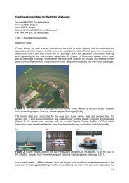
(Figure 1). The current pattern in the outer port of
Zeebrugge is strongly influenced by the tidal cycle.
As such, an accurate and detailed current atlas is of
vital importance for the safe and effective navigation
of shipping into the Port of Zeebrugge.
The current atlas was constructed for the outer port
during spring, neap and average tides. To achieve
this, a strict surveying scheme was created using
Figure 1: The outer Port of Zeebrugge with the survey zones marked by coloured stripes. Adapted from Verwerkingsrapport
Stroming meetcampagnes Zeebrugge [2011].
Hydro12 | 5

(a)
(b)
Figure 2: Survey vessels used for the ADCP measuring campaign, a) MS BEASAC VI, b) MS EB2, c) MS
WALRUS. Adapted from Verwerkingsrapport Stroming meetcampagnes Zeebrugge [2011].
(c)
multiple vessels surveying simultaneously (Figure
2). All vessels were mounted with an Acoustic Doppler
Current Profilers (ADCPs), which measured
current speed and direction using broadband technology
and bottom track functionality.
Low current speeds, a diffuse sediment layer and
choppy wave conditions made measurements in the
outer port of Zeebrugge a challenge. Furthermore,
shipping activities in this busy port required survey
vessels to veer off course, leading to gaps in the surveying
scheme and a disruption to acoustic signals.
To solve these challenges, Aqua Vision BV developed
two novel solutions for port based surveying.
First, a new data processing approach optimized
data quality by using a combination of bottom
tracking and dGPS. In this way, an optimum current
speed solution could be derived, ensuring accurate
and precise current speed and direction data. Second,
a central surveyor station was set up using a
remote desktop connection to all survey vessels, in
order to optimize real-time planning and anticipation
of shipping activities.
METHODS
The port was split into several distinct zones (Figure
1). Three survey vessels were equipped with ADCPs
(Teledyne RD Instruments) and deployed to simultaneously
survey during spring tide, neap tide and
average tide. For each tidal type, three boats surveyed
all zones in two days of 13-hour measurements.
Data acquisition and reprocessing were performed
using the data acquisition software package ViSea-
Figure 3: Current patterns during high spring tide. Adapted from Stroomatlas Haven van Zeebrugge [2011].
6 | Hydro12

DAS (Aqua Vision BV), affording real-time synchronization
between ADCP, GPS, gyro compass
and motion sensor. Data quality control, presentation
and current atlas generation was carried out
using ViSea-DPS (Aqua Vision BV).
RESULTS AND DISCUSSION
A representation of the current patterns in the outer
port of Zeebrugge during spring, neap and average
tides was created to aid shipping and navigation in
this busy port (Figure 3).
The series of current maps provide insight in the 3D
current patterns in the outer port of Zeebrugge. The
most striking current patterns were visible during
the spring tide. In the initial phase of high tide the
currents outside the port remain southbound. This
reflects the inertia of the westwards flowing water
mass. As such, water enters the port basin from the
south side of the port entrance and current velocities
at the entrance are relatively weak. Two hours
before high tide, currents outside the port have
turned and start filling both Zeebrugge port. This
coincides with the onset of the steepest part of the
water level curve, which cause steep spatial water
level gradients between the sea and the port basin.
This results in high current velocities throughout
the port system. Water enters the port at the northeastern
side of the entrance and flows to the tip of
the Leopold II-dam. This creates a jet-like system
with the highest current velocities directed inward
on this line. To the east and west, a return flow is
created, causing a double eddy system in the outer
port basin.
At the peak of high tide, the basin is completely filled,
while currents are still strongly flowing northward
at sea. The double eddy system however con-
tinues swirling inside the outer port basin. At this
time, strong vertical shear also exists. An example
can be found in the outer part of the port basin, just
inside the port entrance, northeast of the Wielingendok
(Figure 4). A seaward return flow is active near
the water surface (Figure 4a) while water is flowing
inward near the bottom (Figure 4a).
With the falling of the tide, the double eddy system
is pushed seaward until it has vanished at 4 hours
after high tide. From this time onward, water is
steadily flowing out of the basin until low tide is
reached. Current patterns at mean tide and neap tide
are similar but with smaller current velocities.
Figure 5: Current pattern at 4hr 40 before spring
high tide in the entrance of Wielingendok. Even
though current velocities are small, a clearly visible
eddy has accurately been mapped.
The high accuracy of the measurements becomes
evident when viewing the current pattern in the
entrance of Wielingendok at 4hr40 before high tide
(Figure 5). Although the current velocities are extremely
low (0.1 knots on average), an eddy is clearly
visible, having developed due to water entering at
the south side of the Zeebrugge port entrance.
MOVING BED
(a)
(b)
Figure 4. Current pattern at spring high tide just
inside the port basin at (a) 2 m depth and (b) 16 m
depth.
Low current speeds are inherent to port basin environments.
Under such conditions the differential
between current speed and vessel speed becomes
a crucial factor in determining the precision of the
data. During the data validation step the measured
current speeds are corrected for vessel speed. In this
Hydro12 | 7

(a)
Figure 6: The application of a combined Bottom track/GPS correction for vessel speed, a) Velocity magnitude
data before correction, b) Velocity magnitude data after correction. Adapted from Verwerkingsrapport
Stroming meetcampagnes Zeebrugge [2011].
(b)
case bottom tracking is always the preferred method
due to its direct synchronization with the ADCP.
However, local sediment dynamics can sometimes
disrupt bottom track detection, either due to a moving
bed or no bottom detection.
This was case in the Port of Zeebrugge, where the
muddy seabed at times became too diffuse to detect
the bottom. When this occurs, bottom tracking is
no longer available and GPS has to be used, with a
resulting decrease in measurement precision associated
with synchronisation issues. This results in
sub-optimal current speed data. A new current speed
correction method was developed based on a combination
of bottom track and GPS data.
Vessel speed is measured dually by Bottom Track
and by RTK. The speed variations are combined
by making use of a low and high pass algorithm,
speed variations with a period 10s
is taken from the RTK. This combination corrects
for both moving bottom and ships movements. In
the absence of a moving bottom the bottom track is
used exclusively. In Figure 6a, the uncorrected current
speed data is shown. After applying the highlow
pass filter method, a clear improvement is seen
in the data (Figure 6b).
CENTRAL SURVEYOR STATION
Any approaching shipping in this busy port not only
requires a survey vessel to veer off track, but can
also disturbs the acoustic signal from the ADCP.
Ultimately, this results in poorer data, time delays
and gaps in survey coverage. One innovative solution
was found in the creation of a central surveyor
station in the Eurosense office in Zeebrugge (Figure
7). Here, a surveyor oversaw the survey activities
of all three boats via a remote desktop connection
with each onboard survey PC. At the same time, the
surveyor kept a close eye on shipping activity via
www.marinetraffic.com. In this way the central surveyor
could anticipate impending survey disturbances
and relay a new survey strategy to the onboard
surveyor and skipper - resulting in increased safety
and an optimised survey strategy.
Figure 7: Central Surveyor Station in Eurosense office, Zeebrugge.
8 | Hydro12

With the advent of high speed mobile internet it is
now possible to remotely operate survey software.
With a central surveyor station, like that used in
Zeebrugge, are we seeing the precursor of remote
surveying?
CONCLUSION
A current atlas has been created for the port of
Zeebrugge during spring, neap and average tides
to aid shipping navigating and safety on approach
and within the outer port. This was achieved using
3 survey vessels measuring simultaneous over a 13
hour period, per tidal condition. Each survey vessel
was mounted with an ADCP. Current patterns in
the outer port show some interesting features, for
example, a delayed response to rising tides, the creation
of a double eddy system within the outer port
and eddy systems even at very low current velocities.
Due to local sedimentary conditions, a novel
new method was used to correct the vessel speed
data. To improve planning and anticipation during
multi-vessel surveying a central surveyor station
was set up using high speed mobile internet.
BIOGRAPHIES
Pim VAN SANTEN is now a researcher water
systems at Waterschap Aa en Maas. He received his
MSc in Physical Geography from Utrecht University,
after which he spent several years as a researcher
in sediment dynamics. At Aqua Vision BV he was
involved in data analysis and processing.
Shauna NI FHLAITHEARTA, currently a data analyst
at Aqua Vision BV, completed her BSc (Hons)
in Earth Sciences at the National University of Ireland,
Cork, and her MSc in Earth Systems Science
at Wageningen University and Research Center.
She then spend several years conducting research in
marine biogeochemistry before joining Aqua Vision
BV in 2010, where she is involved in data processing
and communications.
acoustics before he joined Aqua Vision. At Aqua
Vision he develops hydrographic data acquisition
software.
Frans CLAEYS, a senior project manager of Eurosense,
received his Master of Science degree in
electronics and control at the University of Louvain
in 1982. After his military service he started with
Eurosense in 1983 in the hydrographic department
in Zeebrugge. He is experienced in accurate positioning,
attitude determination, data acquisition and
digital signal processing techniques.
Hans POPPE received his MSc in Physics at the
University in Brussels in 1996 and his MSc in applied
physics in 1999 at the University of Delft.
From then on he started working for hydraulic and
civil engineering consulting agencies, until the end
of 2006 when he started to work as Project Engineer
of Tide and Currents at the Coast Division of the
Flemish government. In this job he is responsible
for the various aspects involving tide and currents
along the Flemish coast and on the Belgian continental
shelf.
CONTACT DETAILS
Jeroen AARDOOM
Aqua Vision - THE NETHERLANDS
Email: j.aardoom@aquavision.nl
Web site: www.aquavision.nl
Frans CLAEYS
Eurosense – BELGIUM
Email: info@eurosense.com
Web site: www.eurosense.com
Jeroen AARDOOM, a senior R&D associate at
Aqua Vision BV. He received his MSc in Physics
from Utrecht University, specialisation computational
science and physical oceanography. He worked
at TNO Physics and Electronics Laboratory on the
use of radar remote sensing data for underwater
Hydro12 | 9

10 | Hydro12

Towards New Standards of Competence for Hydrographers and
Nautical Cartographers
Andrew ARMSTRONG, United States of America
National Oceanic and Atmospheric Administration
University of New Hampshire Joint Hydrographic Center
Ron FURNESS, Australia
IIC Technologies Ltd
Gordon JOHNSTON, United Kingdom
Venture Geomatics Limited
Nicolas SEUBE, France
École Nationale Supérieure de Techniques Avancées Bretagne
Lysandros TSOULOS, Greece
National Technical University Athens
Topic: The Hydrographic Profession
ABSTRACT
Expectations and demands for education and
training and the achievement and maintenance of
core and new competencies in the hydrographic
community are changing apace. The accepted
international minimum competency standards for
hydrographic surveyors and nautical cartographers
have served the profession well, but are presently
under review against these changed expectations.
Community participation will be critical as the
standards deal with and address the changes,
ever mindful of the need for effective delivery of
education and training across the wider profession.
INTRODUCTION
The FIG/IHO/ICA International Board for Standards
of Competence (IBSC) for Hydrographic Surveyors
and Nautical Cartographers (hereafter referred as
“the Board”) have guided the delivery of education
and training for Hydrographers and nautical
cartographers since it was formed in 1977.
The Standards, as promulgated in IHO Publications
S-5 [IHO, 2011] and S-8 [IHO, 2010] (formerly
M-5 and M-8), recognize two levels of hydrographic
(or cartographic) competence—Category A and
Category B. The current Editions of S-5 and
S-8 can be downloaded from the IHO website.
Category A programmes offer a comprehensive and
broad-based knowledge in all aspects of the theory
and practice of hydrography or nautical cartography.
Category B programmes provide the practical
comprehension, along with the essential theoretical
background, necessary for individuals to carry
out the various hydrographic survey or nautical
cartographic tasks.
The standards have been structured so that Category
B programs provide technical education to support
a set of fundamental and practical competencies.
Category A educational programs must include
all the Category B competencies plus additional
detailed-level competencies. This means that
Category B is a subset of Category A, and the S-5
S-8 standards are structured accordingly. Along
with hydrographic and cartographic technology,
the personnel and training needs of Hydrographic
Offices and the hydrographic industry have evolved
considerably since 1977.
THE BOARD, THE STANDARDS AND THE
RECOGNITION PROCESS
The Board comprises ten Members representing
the three constituent organizations: FIG, the
International Federation of Surveyors (4); IHO, the
International Hydrographic Organization (4); and
ICA, the International Cartographic Association
Hydro12 | 11

(2). The Board Secretariat is provided from the
IHO. The present Board comprises a cross section
of experts representing the broader hydrographic
community and are from Australia, France,
Germany, Greece, India, Malaysia, New Zealand,
Trinidad and Tobago, United Kingdom and the
United States. The Secretary brings his experience
from Brazil. The Board meets annually and it is
charged with maintaining S-5 and S-8 standards and
considering course curricula submissions against
these standards for recognition. Recognition of
courses is granted only when those curricula meet
the appropriate requirements. A list of those courses
recognised is available online [IHO, 2010(2)].
The Board’s operations are governed by its
published Terms of Reference and Rules of
Procedure [IHO, 2011(2)] as ratified by the
constituent organizations. The decisions made by
the Board are independent. A small submission
fee and annual fee are levied on submitting
organizations, which assists in funding the Board’s
activities although Members largely fund their own
participation.
The Board has recognised various pressures for
change that will be revisited below and is in the
process of reviewing both standards in order
to modernise them and better reflect modern
requirements for achieving qualified hydrographic
surveyors and nautical cartographers at various
levels of competence.
Courses seeking recognition are submitted by
competent educational and formal training bodies
by 31 December each year. The Board meets
subsequently after each member has reviewed
submissions and in plenary the Board considers
each submission. Once recognised, course
recognition remains valid for six (6) years assuming
its delivery continues. After six years a new
submission is required.
The Board does not recognise individuals but
has introduced minimum requirements by which
it will recognise national or regional schemes,
which in turn recognise or accredit individuals.
Such schemes typically require qualified persons
to remain current through access to continuing
professional programs.
The Board will begin the process of changing the
Standards with S-5. The S-5 Standards indicate
the minimum degree of knowledge and experience
considered necessary for hydrographic surveyors,
and provide a set of programme outlines against
which the Board may evaluate programmes
submitted for recognition.
Early editions of M-5 were significantly changed
with the publication of the fifth edition, which
represented a fundamental change of approach in
order to make the Standards more applicable to the
different requirements for hydrographic surveyors
in government and industry. The fifth edition
Standards provided basic and essential subjects that
are required for all hydrographic surveyors and a
choice of three options for specialization in Nautical
Charting Surveys, Surveys for Coastal Zone
Management or Industrial Offshore Surveys.
The sixth edition incorporated a change in format,
to facilitate easier cross-referencing between
syllabus topics and programmes which were
submitted for recognition and also included
minor changes in content to eliminate duplication
of subject matter and to reflect the evolution of
technology. The seventh edition eliminated the
distinction between Full/Academic recognition and
increased the emphasis on developing techniques
of GPS, multibeam sonar systems and ECDIS.
The eighth edition eliminated the Specialisms and
re-structured the Syllabus in two different parts:
the “Minimum Standards”, including Basic and
Essential Subjects and the “Optional Units”.
The ninth edition (2001) provided a better definition
of the three levels of knowledge (Fundamental,
Practical, Detailed) identified in the syllabus.
Nautical Science was moved to the Basic
Subjects, and was modified to reflect the minimum
knowledge required by an hydrographic surveyor.
This edition contained a more detailed description
of each subject, which were divided into Category
A / Category B and Category A-only learning
objectives.
The tenth edition makes changes to Section 3
“Submission of Courses”, introduces a new
Appendix V “Annual Assessment Report” and
also reflects the change of the Board’s name
which became “FIG/IHO/ICA International Board
12 | Hydro12

on Standards of Competence for Hydrographic
Surveyors and Nautical Cartographers” as agreed
during the 31st Meeting.
In 2009 the IHO restructured its publications and
the M-5 Standard was renamed S-5. The eleventh
edition includes a new and expanded section
relating to the recognition of Schemes that certify
the competency of Individuals beyond their formal
education and training.
The present Standard S-5 comprises:
• Educational and training programs at two
levels:
• Category A
• Category B
• 3 Knowledge Levels: Fundamental, Practical &
Detailed
• 2 Groups of Subjects: Basic & Essential
• 7 options (Nautical charting, Hydrography
to Support Port Management and Coastal
Engineering, Offshore Seismic Surveys,
Offshore Construction Hydrography, Remote
sensing, Military Hydrography, Inland Waters
Hydrography)
• Individual Recognition Schemes
Category B is currently defined as a programme that
provides a practical comprehension of hydrographic
surveying for individuals - along with the essential
theoretical background - with the skill to carry out
the various Hydrographic surveying tasks.
• Example competency: “Explain the principles of
various types of water level gauges and poles.
Describe characteristics of river, coastal and
offshore water level gauges. Install and operate
water level gauges and poles”.
Category A is a programme which provides a
comprehensive and broad-based knowledge in all
aspects of the theory and practice of hydrography
and allied disciplines for individuals who will
practice analytical reasoning, decision making and
development of solutions to non-routine problems.
• Example Competency: “Evaluate and select
appropriate instruments and sites for water
level monitoring. Calibrate analogue and digital
recording water level gauges. Evaluate sources
of error. Apply appropriate corrections”.
Individual recognition schemes are regional or
national bodies that evaluate, certify, and track
the competence of individual hydrographers. S-5
sets out standards of organization and content
for these schemes. Recognized schemes may
certify individuals at levels other than Category
A, or B, but only individuals who have completed
a Category A or B course may be certified as
Category A or B Hydrographers. At the May
2012, 35th meeting of the Board in Buenos Aires,
Argentina, the Board recognized the Australasian
Hydrographic Surveyors Certification Panel
(AHSCP) as the first approved scheme of individual
hydrographers competence.
NEW CHALLENGES IN HYDROGRAPHY
EDUCATION AND TRAINING
It has become evident to the Board that there are
a number of influencing factors that bring about
imperatives for change in the way hydrographic
surveyors and nautical cartographers are educated
to meet modern hydrographic practice and products
requirements.
New use of the seas has shifted the hydrographic
products from those intended mainly for navigation
safety to a wide variety of deliverables, motivated
by emergent fields like energy production (wind
farms, marine turbines, etc.), marine environment
understanding and protection (habitat mapping,
coastal erosion monitoring, coral reef mapping,
etc.), remote sensing bathymetry (using bathymetric
LiDAR, AUVs, ASVs, or satellite data). Field
operations are and will be conducted in the near
future at a wide variety of scales: from detailed port
infrastructure inspection survey to regional satellite
bathymetry.
To respond to these new challenges, equipment
and software are becoming more and more
sophisticated and automated. We are now dealing
with hydrographic systems (being by essence
kinematic mapping systems), composed of complex
sensors incorporating a high level of technology and
embedded software.
The increasing complexity of field operations
with added requirements for skills such as
project management, financial acuity and broader
professional aptitude with greater cross discipline
experience and exposure - in some cases without
Hydro12 | 13

actual seamanship skills (LiDAR operations perhaps
or port based operations) requires consideration and
definition.
The increasing amount of data that are collected
need to be processed (cleaned, controlled,
generalised), and integrated in marine geospatial
data management systems. Data processing
and management systems incorporate advanced
numerical methods enabling the hydrographer
access to high-level models built from multi-sensors
raw datasets. These stretch the knowledge required
by hydrographers.
Technology in the field increasingly requires better
qualified technicians and operators who may
not be required to go further than a consolidated
Category B programme. This apparent conflict
is compounded by the increase in demand for
competent hydrographers. More and more there is
little time available as busy individuals attempt to
balance their work and leisure life. The challenge in
its broader sense is to be able to provide adequate
technical foundations combined with appropriate
practical exercises but without removing the
individual from their work environment for too long
a period or requiring the educational organisation
to invest in complex and expensive equipment that
may only be used a few weeks per year.
The influence of blended, direct and distance
learning initiatives is beginning to have an impact.
The growing perception now is that modular, short
educational courses coupled with intensive time
on practical and field work may offer a solution
that combines the desires of individual and course
providers through a flexible approach to the
selection, completion and assessment of course
elements making up. For the Board these must be
of adequate time and rigour as well as accumulating
into a comprehensive cover of any minimum
Standards.
In the framework of these new challenges the
Board has decided to strengthen the importance of
programme review as a process for evaluating and
continuously enhancing the quality and currency
of programmes. The evaluation will be conducted
through a combination of self-assessment, followed
by peer on-site consultation by members of the
Board, for the mutual benefit of all parties. In
addition, a visit will serve to raise the profile of
hydrography and nautical cartography nationally
and regionally.
TOWARDS NEW STANDARDS
Early thoughts of the Board suggest the separation
of the present Category B and Category A
requirements and a future separate path of
development for each. In view of the foreseen
challenges in hydrography and nautical cartography,
the Board believes that a fundamental change to the
structure of the Standards is appropriate. The Board
is in the process of developing a new structure for
S-5 and S-8 that will separate the Standards for
Category A and Category B programs. Standards
for each category will be designed and developed
independently.
Category B standards will be aimed at the
basic educational and training requirements for
hydrographic technicians and field hydrographers
(S-5), and nautical cartographers (S-8). Category
A standards will be aimed at the theoretical
educational and foundational background necessary
for Hydrographers/Nautical Cartographers-In-
Charge and hydrographic/cartographic managers
who will develop specifications for surveys
and charts, establish quality control and quality
assurance systems, and respond to the specific
requirements of a full range of hydrographic/
cartographic projects.
For both Category A and Category B standards, the
ability to conduct or operate hydrographic surveys
in the field or utilize hydrographic/cartographic
databases to compile and produce charts, remains
an essential competence, and thus an essential part
of education and training through the necessity of
practicals (field exercises/projects).
The Board expects to complete new S-5 standards
by 2014, and intends to communicate about this
process before the final release of the new S-5 and
S-8.
THE DEVELOPMENT PATH
The Board will need to grapple with various and
varying impacts as it works through how best it
can provide guidance for minimum standards into
the future. Anecdotally, at least, it is clear to the
Board that the demand for qualified hydrographic
surveyors and nautical cartographers is increasing.
14 | Hydro12

Simultaneously, as evidenced partly by the creation
and introduction of professional bodies that review,
certify and track the competences of practitioners
within the industry, there is an increasing clamour
for qualified competent hydrographic/cartographic
personnel. Many hydrographic contracts, by way
of example, now demand evidence of formal and
appropriate hydrographic/cartographic qualification
and competence as a consideration in the evaluation
of tender responses. Naturally, this is accompanied
by demand from the personnel themselves for
opportunities to study and to continue their skill
refreshment within accredited and recognised
programs that provide evidenced continuation
of individual, and thus consequently, corporate,
professional competency.
Those personnel entering the profession do not find
it easy in at least some parts of the world to find
courses that suit their needs. Not everyone seeks a
military career that was hitherto often the genesis of
many a longer term successful hydrographic career.
The Australasian region, for example, has struggled
to sustain its civilian hydrographic training courses
and even recognised courses have foundered for a
number of reasons. A new attempt to provide such
initial training opportunities is presently under way.
The reasons for the difficulty of maintaining
courses are varied, but for those bodies offering
them, it all boils down to the critical number of
students applying for the course - or rather - a lack
of sufficient numbers to sustain such specialist
and high cost training and education. Factors
affecting student numbers include costs, time,
and changing expectations on the parts of both
students and employers. These are high on the lists
of influencing factors for those who make their
difficulties known.
Industry-wide, and broadly speaking, the
employment of hydrographic professionals is
changing from life-time careers to project and
contract employment which frequently requires
skill-set refreshment and new technology-based
competencies which sometimes are found to
be lagging in established courses. Longer term
practitioners require access to change learning
paradigms. Students bring changed expectations
therefore, given that they must work in such an
industrial environment. Expectations are high
among modern students: they are typically computer
literate and modern survey equipment competent,
but require rapid and often short term results for a
specific instance of employment.
Employers, on the other hand, have complementary
expectations that they will either find such students
in the market place or will take on board their
own training in order to meet the exigencies of
the tenderer’s expectations and project demands.
Demand for immediately functional skill sets
is high. Increasingly, the market place cannot
immediately deliver.
The educational world itself is in turn influenced
by changing technological and methodological
imperatives. The older forms of institution of
university or national agency are being challenged
to deliver. Connectivity and the introduction of
so-called e-learning methods, blended learning
techniques, webinars, e-seminars, e-meetings
and the like, have naturally attracted the attention
of hydrographic agencies and companies and
their staff and it is not surprising that, given the
offshore nature of much of the industry, attempts
are being made to harness the better technologies
and methods to achieve the requirements outlined
above. The potential of these forms of program
delivery are beguiling and seemingly cost-effective
in their promises however their successful delivery
largely still needs to be proven.
All components of the hydrographic profession face
challenges as to how best to ensure the continuance
of the high standards and how best to ensure the
continuation of best practices based on minimum
standards of competence world-wide. A cooperative
approach will best deliver future guidance to all.
CONCLUSIONS
Attitudes toward training and education are
changing. The hydrographic profession is not
immune from such broader pressures. There are,
however, some unique aspects of hydrographic
surveying that impact on how training and
education can best be delivered. While the S-5
approach has stood the profession in good stead
and is generally well recognised throughout the
hydrographic world, there is sufficient evidence to
suggest it needs a complete review and overhaul to
Hydro12 | 15

ing it in line with current expectations of how to
achieve community-wide best practice for minimum
standards of competence. The Board, in facing the
challenges outlined above, anticipates posting its
draft revisions online for stake-holder feedback and
contribution. This paper itself is to be considered a
part of this process.
REFERENCES
IHO—International Hydrographic Organization.
2011. “Standards of Competence for Hydrographic
Surveyors,” Publication S-5, 11th Edition,
Version 11.0.1—May 2011, accessed 24 June
2012. http://www.iho.int/iho_pubs/standard/S-5_
Ed_11.0.1_06May2011_Standards-Hydro.pdf
IHO—International Hydrographic Organization.
2010. “Standards of Competence for Nautical
Cartographers,” Publication S-8, 3rd Edition, 2010,
accessed 24 June 2012.
http://www.iho.int/iho_pubs/standard/S_8_3rd_
Jan_2011.pdf
IHO—International Hydrographic Organization.
2010(2). “List of Recognized Courses
Hydrography,” May 2010, accessed 24 June 2012.
http://www.iho.int/mtg_docs/com_wg/AB/AB33/
LISTMAY10.pdf
IHO—International Hydrographic Organization.
2011(2). FIG/IHO/ICA International Board (IB) on
Standards of Competence, “Terms of Reference,”
Revision 1, 2011, accessed 24 June 2012.
http://www.iho.int/mtg_docs/com_wg/TOR/IBSC_
TorsRops_2011-rev1.pdf
BIOGRAPHIES
The authors have a wide variety of hydrographic
and cartographic experience in government,
academia, and private industry. All are members of
the FIG/IHO/ICA International Board on Standards
of Competence for Hydrographic Surveyors and
Nautical Cartographers.
16 | Hydro12

The CARIS Engineering Analysis Module -
Assisting in the Management of Queensland’s Waterways
Owen CANTRILL, Australia
Maritime Safety Queensland
Daniel KRUIMEL, Australia
CARIS Asia Pacific
Topic: Innovations in processing techniques
INTRODUCTION
Maritime Safety Queensland (MSQ) is a division of
the Department of Transport and Main Roads within
the Queensland State Government. MSQ’s role is to
protect Queensland’s waterways and the people who
use them - providing safer and cleaner seas. Within
the corporate structure of MSQ, the Hydrographic
Services section carries out hydrographic surveys
on behalf of clients. Current clients include
North Queensland Bulk Ports (Ports of Hay Point,
Weipa, Abbot Point and Mackay), Ports North
(Cape Flattery, Thursday Island), Gladstone
Ports Corporation and Boating Infrastructure and
Waterways Management (recreational boating
facilities). These various sites are spread over
1700Nm of coastline.
OVERVIEW OF OPERATIONS
MSQ utilize a variety of survey equipment, such
as a Kongsberg Simrad EM 3002D multi beam
echo sounder, Klein 3000 Sidescan, Starfish 452f
sidescan, SEA Swath plus 234 kHz interferometry
system, Echotrak MK III dual frequenciy single
beam, Deso 300 single beam, Applanix POS MV
320, Applanix POS MV Wavemasters and Lecia
RTK DGPS. Surveys range from boat ramps that
integrate land survey and a small hydrographic
component, through to high precision surveys for
Under Keel Clearance systems.
A permanent installation of the EM3002D exists on
the vessel QGNorfolk, with other mobile systems
deployed on vessels of opportunity, such as the QG
Bellara used during rapid response surveys in the
2011 Brisbane floods.
MSQ ensures a high quality of work through the use
of experienced and competent personnel. There are
six surveyors certified at Level 1 by the Australasian
Hydrographic Surveyors Certification Panel
(AHSCP) and five surveyors (including graduates)
that work under direct supervision.
In an effort to improve acquisition to processing
ratios, MSQ first incorporated CARIS Ping-to-Chart
products into their workflow early in 2009, turning
to HIPS and SIPS for processing their bathymetric
data. Later that year, BASE Editor was also brought
on board to assist in bathymetric data compilation
and QC. Staff from MSQ have stayed well versed
in the latest functionality for the software packages
through participation in open training courses held
in the region by the CARIS Asia Pacific office.
After attending a training course on the new
Engineering Analysis Module (compatible with
BASE Editor) in August of 2011, MSQ sought to
expand on their current functionality and utilize the
new module to assist them in the management of
their ports and waterways throughout Queensland.
THE ENGINEERING ANALYSIS MODULE
The Engineering Analysis Module features under
the ‘Analysis’ pillar of the Ping-to-Chart workflow,
as part of the Bathy DataBASE suite of products.
Recognising the fact that different users have
different requirements, Bathy DataBASE is a
scalable solution.
In order to provide more functionality for users
in the ports and waterways environment, the
Engineering Analysis module was introduced to the
Bathy DataBASE product suite. The module works
with either BASE Editor or BASE Manager, and
includes many functions migrated from an existing
CARIS application (BEAMS - Bathymetry and
Engineering Management System). These functions
include volume computations, shoal management,
Hydro12 | 17

conformance analysis and reference model creation
and maintenance.
VOLUME CALCULATION METHODS FOR
HYDROGRAPHIC SURVEYING
The calculation of volumes in hydrographic
surveying is frequently used in dredging
applications and reservoir analysis (for example,
sedimentation). A number of different methods
can be utilized in determining a volume. The ‘best’
method to use is determined by factors such as the
technique of sounding for the data (single beam,
multibeam, LiDAR etc.) and also the nature of the
material (smooth, sandy bottom is quite different to
an undulating, rocky terrain).
“Accurate volume estimates are important for the
choice of dredging plant, production estimates and
ultimately project costs. “ (Sciortino J.A., 2011)
In addition to the volume of material, the type of
material is another important factor. The cost of
dredging rock will be much higher compared to the
same amount of material in sand.
End Area Volumes
End Area volumes have been derived from landbased
methods used in railroad and roadway
construction. They involve calculating the volume
from cross sections of a channel, surveyed at regular
intervals (see Figure 1). The key components in
computing the volume are the cross sectional area
(an average is taken of the two areas) and the length
between the cross sections. This method assumes
that the cross sectional area is relatively constant
between two successive cross sections. If this
assumption is not true, the volume produced will
realistically just be an approximation.
TIN Volumes
Triangulated Irregular Network (TIN) Volumes are
based on the true positions of depths to calculate
the volume of a surface. This calculation involves
modelling the surface as a collection of small
planes. TIN’s can either be derived from a gridded
bathymetry source (i.e. surface) or from a point
cloud. One advantage in using the TIN method
(particularly for point data) is that the true position
of the source depths will be utilized in the volume
calculation. This is the historically preferred
method for most dredging type applications where
volume is critical.
Hyperbolic Volumes
For this method, a hyperbolic cell is created from
the centres of every four adjacent grid cells. The
depths from the grid cells are used as the depths
for the corners of the hyperbolic cell. For this
calculation, the surface is modelled as a collection
of hyperbolic paraboloid sections, with a hyperbolic
paraboloid created to smoothly pass through the
points of each hyperbolic cell (see Figure 2). This
gives a smooth approximation of the surface and
good volume results, but is processing intensive and
can be time consuming.
Rectangular Volumes
Figure 1: Calculation of End Area Volumes (USACE, 2001).
18 | Hydro12

VOLUME COMPARISONS
Figure 2: Representation of the hyperbolic paraboloid
volume method.
In this method, a single depth value from each
cell (or bin) in the surface is used to calculate the
volume. The surface is modelled as a collection
of disjointed rectangular prisms, with the depth for
each grid cell becoming the depth of the prism (see
Figure 3). In comparison to the previous hyperbolic
method, this results in a much more ‘simple’
volume calculation which is processed much faster,
however the accuracy of the computed volume may
not be as reliable.
One limitation on the rectangular volume method is
the inability to perform a volume calculation against
a sloped or non-horizontal surface in a reference
model (for example the bank of a channel). This is
because by definition, a rectangular prism cannot
have a sloped edge, so only horizontal reference
surfaces are supported.
Figure 3: Representation of the rectangular volume
method.
As previously outlined, there are a number of
different methods available to the hydrographer for
volume determination. So this leads to the next
question - which method should be used? This
will largely be dependent on what technology is
available to conduct the survey. If the user only
has access to a single beam echo sounder, they will
be limited to end area volumes and TIN volumes.
For a full density multibeam survey, rectangular
and hyperbolic volumes can also be taken into
consideration.
The nature of the seafloor (or riverbed/reservoir)
could be another factor in determining which is the
most suitable volume method to be used. If the
bottom topography is smooth (such as with sand),
hyperbolic volumes, which produce a smooth
estimate of the terrain using constructed hyperbolic
paraboloids could yield the best results. For a
harsher, rocky terrain, TIN volumes utilizing the
true positions of each depth may be the most robust
answer.
Case Study in Weipa
In order to test the results produced by the various
methods of volume calculation, a case study was
carried out using survey data collected by MSQ at
the Port of Weipa in October, 2011. The data was
provided as an ASCII XYZ file that had already
been binned at 1m. A reference model for the Port
of Weipa was also used in the calculations. The test
area used is a section of channel located just to the
east of beacons 7 and 8 in the south channel.
Volumes were calculated in the test area to
determine the amount of material that would need to
be removed to bring the channel down to a declared
depth of 16m (Note: this is just an arbitrary value
chosen for testing purposes). The methods used for
comparison were hyperbolic, rectangular and TIN
volumes. Simulated end area volumes were also
calculated by extracting profiles from the multibeam
bathymetry at intervals of 25m, 50m and 100m.
The results can be seen in Table 1. (Note: In this
case, the hyperbolic volume has been used as the
benchmark for determining volume difference and
error for other methods. This does not mean that
there is zero error in the hyperbolic volume result).
Hydro12 | 19

METHOD VOLUME m 3 DIFFERENCE m 3 VOLUME ERROR %
Hyperbolic volume 794,912.5 0 0
Rectangular volume 805,090.2 10,177.7 1.280
TIN volume 798,654.2 3,741.9 0.471
End area 25m interval 803,019.1 8,106.5 1.020
End area 50m interval 802,755.3 7,842.7 0.987
End area 100m interval 802,022.8 7,110.2 0.894
Table 1: Comparison of volume results for the test area in Weipa
The results displayed in Table 1 yield some
interesting results. As could be expected, the two
volumes closest to each other are the hyperbolic and
TIN volumes. What is probably most surprising
are the results achieved through the use of end
area volumes. One would generally assume that
profile spacing would be inversely proportional to
the volume difference/error (i.e. the lesser distance
between profiles, the greater the accuracy of the
computed volume). This is not reflected in these
results, where the error actually decreases as the
interval increases. This may be due to the nature of
the seabed. The data used was a pre dredge data set
following the wet season. The channel is typically
smooth and shaped in a reasonably consistent V
shape due to the amount of siltation and the effect
of significant shipping movements which assist in
keeping the centreline clear of siltation.
Validation of Case Study
As the results produced in the Weipa case study
did not reflect expected results, an additional
independent case study was sought out. One was
found by Dunbar J.A and Estep H of the Baylor
University Department of Geology (BU) in Texas,
USA. The project undertaken by BU was to study
the hydrographic surveying methods utilized by
the Texas Water Development Board (TWDB)
in determining water and sediment volume in
reservoirs throughout Texas. Whilst the project
also investigated sub bottom profiling and sediment
surveys, the volume comparison was carried out in
Lake Lyndon Baines Johnson (LBJ), a Highland
Lake on the Texas Colorado River.
As part of the project, Hydrographic Consultants
Inc collected and processed a multi-beam survey
in Lake LBJ. In order to evaluate the influence of
survey profile spacing on volume accuracy,
“BU extracted simulated profiles at spacing’s
ranging from 100 to 2000 ft from a high-density
multi-beam survey collected by an independent
contractor. Volume calculations based on the
extracted profile sets were compared to the volume
based on the full multi-beam survey. “ (Dunbar, J.A,
Estep, H, 2009)
The results produced in the study by BU can be
seen in Table 2. They are also shown graphically
in Figure 4. When extracting the profile sets to
produce simulated volumes, BU did this in two
runs (Run 1 and Run 2). This meant that for each
simulated profile spacing, two independent sets
of profiles were extracted from the multibeam
bathymetry.
By undertaking a statistical analysis of the BU
Volume comparison results, values from Run 1 have
a coefficient of correlation of 0.884 and 0.936 for
Run 2. This indicates a strong positive correlation
between profile spacing and volume error, which is
what we would generally expect. However despite
the strong correlation, there are inconsistencies in
the data. Such as the very low value of 0.14 % for
1000 ft profile spacing in Run 1, and a difference
of 0.696% in Run 1 and Run 2 error for 300 ft
profile spacing. This is because the Volume Error of
0.718% for 300 ft profile spacing in Run 1 is higher
than expected in contrast to other results.
20 | Hydro12

Table 2: Results of BU Volume Comparisons (Dunbar, J.A, Estep, H, 2009)
From
these results, a conclusion can be drawn that hydrographic surveys. As part an evaluation for the
when
increasing the population size of our sample Engineering Analysis Module in 2011, MSQ ran a
dataset, the error values do display a tendency for comparison of TIN volume computations using the
strong positive correlation. In the Weipa Case module against their existing capability. Results
Study, the population size was only three (25m, from the comparison can be seen in Table 3. The
50m and 100m spacing) so these results were Engineering Analysis Module produced the same
not apparent. If further intervals were added and TIN volume results, in less time across all cases, as
multiple runs (as in the BU example), perhaps we well as having the ability to compute a volume for
could expect to see similar results.
the entire channel (which the existing capability was
not able to achieve).
It could therefore be argued that while there is
a trend for volume error to increase with profile CONCLUSION
spacing, for any given dataset based on one set of
profiles
(i.e. a single beam survey) the accuracy of The Engineering Analysis Module is able to
the volume is essentially down to ‘luck.’ In their greatly assist users in managing Ports and
report, Dunbar J.A and Estep H state that
Waterways through the use of conformance
“Reducing
the profile spacing to less than 500 ft analysis, sophisticated volume computations, shoal
does
not guarantee improved volume accuracy. “ detection/management and the creation, editing and
(Dunbar,
J.A, Estep, H, 2009)
maintenance of reference models. When computing
volumes, users should consider what type of volume
VOLUME
COMPUTATIONS AT MSQ
will deliver the most accurate results. While
End Area volumes have traditionally been quite
MSQ
have traditionally used the TIN method widely used, this paper presents evidence that TIN
when
required to compute volumes for their volumes and hyperbolic volumes should be taken
5/7
Figure 4: Scatter plot and 3D line graph of BU volume comparisons.
Hydro12 | 21

Table 3: Volume results and processing times at MSQ
into consideration as they are capable of producing
volume results that are reliable and repeatable.
The Engineering Analysis Module has provided
MSQ with the ability to compute volumes faster
and on much larger data sets than their existing
capability, along with new functionality for
advanced visualization techniques. The ability
to increase the data sets reduces the trade off
historically required between precise volumes (e.g.
0.5m spaced data) with practical processing limits.
(Data generalised to 2.5m)
REFERENCES
Cantrill, O, (2012) General Aspects of Port
Surveying and Shallow Water Bathymetry,
Proceedings of SWPHC Ports & Shallow Water
Bathymetry Technical Workshop, Brisbane,
Australia, March 13-14
Dunbar, J.A, Estep, H, (2009) Hydrographic
Survey Program Assessment Contract No
0704800734, Baylor University Department of
Geology, Waco, TX
Kruimel, D, Fellinger, C, (2011) Bathymetric
Data Management: The Ports and Waterways
Environment, Proceedings of Hydro 2011
Conference, Fremantle, Australia. November
7-10
Sciortino, J.A, (2011) Fishing Harbour Planning,
Construction And Management: Fao Fisheries And
Aquaculture Technical Paper No. 539
USACE, (2001) Hydrographic Surveying,
Engineering Manual 1110-2-1003, United States
Army Corps of Engineers, Washington, DC.
BIOGRAPHIES
Owen Cantrill is a Level 1 Certified Hydrographic
Surveyor having gained certification in 2000. He
gained a Bachelor of Surveying with honours
from the University of Melbourne in 1989. He
is currently employed as the manager of the
Hydrographic Services section of Maritime Safety
Queensland (MSQ).
Daniel Kruimel is an active member of the Spatial
Industry and is currently a member on the SSSI
Regional Committee of South Australia, as well as
the Hydrography Commission National Committee.
At the start of 2011, Daniel took up a role with
CARIS Asia Pacific as a Technical Solutions
Provider.
CONTACT DETAILS
Daniel Kruimel
CARIS Asia Pacific
Level 3, Shell House, 172 North Terrace
Adelaide SA 5000
AUSTRALIA
Tel.: +61 450 802 039
Email: daniel.kruimel@caris.com
Web site: www.caris.com
6/7
LinkedIn account: http://www.linkedin.com/pub/
daniel-kruimel/2b/295/67
Twitter account: @dkruimel
22 | Hydro12

Sediment vs Topographic Roughness:
Antropogenic Effects on Acoustic Seabed Classification
Ruggero Maria CAPPERUCCI, Germany and New Zealand
MARUM, Center for Marine Environmental Sciences, University of Bremen
Department of Earth and Ocean Sciences, University of Waikato
Marine Research Department, Senckenberg am Meer
Alexander BARTHOLOMÄ, Germany
Marine Research Department, Senckenberg am Meer
Topics: Careful marine planning; Geophysics of the marine environment
INTRODUCTION
In recent years, environmental case studies of highly
developed marine areas have become more relevant
[Winter and Bartholomä, 2006; van der Veen and
Hulscher, 2008]: for monitoring both the short- and
long-term human impact on bio- and geo-sphere;
for modelling the effects of such increasing pressure
on ecosystem; as a key tool for environmental and
socio-economic policy and management.
Among the different marine domains, coastal areas
are the most accessible ones and the most difficult to
be studied in detail, due to the complexity of natural
and anthropic processes in action [OSPAR, 2008].
As a consequence, there is an increased demand
for reliable high-resolution mapping tools, less
dependent on expertise interpretation, and therefore
more objective [Cutter, 2003].
In this scenario, the combination of acoustic,
sedimentological and biological data is becoming
the main approach for seabed habitat mapping
studies [Brown, 2011]. Nevertheless, some specific
aspects need further investigations: firstly, the
analysis of acoustic data is still largely dependent on
human expertise [Cutter, 2003]; secondly, repeated
sampling technique is a standard procedure for
biological studies but not a common practice for
sedimentary research; and lastly, the ground-truthing
process by means of sediment samples assumes
that the point-based information can be consistently
extended to the near vicinity of the sampling station.
Besides, the positioning error/uncertainty is often
not even mentioned as a key factor for assessing the
reliability of the final seabed classification.
The latter assumptions have to be proved for
extremely heterogeneous environments, where
anthropogenic impact increases significantly
the disturbance (and, hence, the variability) of
ecosystems.
In our study site of the Jade channel in the
German Bight (southern North Sea) hydrodynamic
conditions, topography, sediments and biocommunities
are tremendously influenced by
multiple human activities. Fishing and mussel
farms are present [Herlyn and Millat, 2000]; the
navigation channel is constantly monitored and
dredged by the local harbour authority (Wasser- und
Schiffahrtsamft Wilhelmshaven – WSA); moreover,
a new container terminal (Jade-Weser Port, http://
www.jadeweserport.de/) is under construction since
2008, with massive land reclamation, dredging
and dumping operations. The Jade channel area
represents, then, a unique site where to test the
reliability of acoustic ground discrimination systems
(AGDS) in a cumulative disturbed area.
The present study aims to address the following
research questions:
1. What is the variability of repeated sediment
samples in a highly heterogeneous environment?
2. How do the positioning error/uncertainty of
sediment samples affect the ground-truthing
process?
3. What drives the seabed classification in the
different acoustic systems?
STUDY AREA AND METHODS
The Jade channel connects the Jade Bay with the
German Bight (southern North Sea), being part
of a wide tidal flat system that includes the Weser
estuary (Figure 1).
Hydro12 | 23

Figure 1 a) The Jade
region, with the Jade-
Weser Port and, in
red, the study area. b)
Location map of the
Jade system. c) close
up un the research
site; white lines: main
acoustic transects,
red crosses: sampling
stations
The northern end (Outer Jade) is a mesotidal
environment (sensu Hayes, 1975), with semi-diurnal
tides ranging between 2.3 and 2.8 m, whereas
the southern part (Inner Jade) is a macrotidal
environment, with the tidal gauge reaching 3.9 m in
Wilhelmshaven.
The sediment distribution shows a general decrease
of the grain-size towards the high-tide line, with the
finest sediments being located in the south-eastern
part of the bay; the Inner Jade is characterized
by the presence of fine sand; fine to medium
sand occurs in the Outer Jade area [Kahlfeld and
Schüttrumpf 2006]. Bedforms are commonly
observed along the tidal inlet.
The research area covers approximately 0.8 km2 in
the Jade Channel, north-east of the Jade-Weser Port,
partially within the old navigation channel. The
water depth ranges between 14 and 26 m.
Acoustic data were collected aboard the R/V
Senckenberg using a Reson Seabat 8125 TM
multibeam echosounder (MBES, 455 kHz), a
dual-frequency Benthos 1624 TM side-scan sonar
(SSS, 110-390 kHz) and a QTC 5.5 TM system
mounted on a Furuno FCV 1000 TM single-beam
echosounder (SBES, 200 kHz). All devices were
deployed simultaneously along 7 main transects (3
approximately east-west and 4 approximately northsouth
oriented). Additional lines were collected for
a complete MBES coverage and a denser SBES
grid. A DGPS system with LRK correction was used
for positioning.
6 stations were sampled (4 replications each) using
a Shipek grab.
Data processing
MBES bathymetric data were processed using
QINSy TM and a final 0.5x0.5 m grid was
computed. DTM generation and seabed features
mapping was done under Global Mapper TM v13.
A set of QTC TM software was used for acoustic
seafloor classification: QTC IMPACT TM for
SBES data, QTC SIDEVIEW TM for SSS data,
QTC SWATHVIEW TM for MBES data, and QTC
CLAMS TM for visualizing and editing classified
data.
QTC IMPACT TM is based on a statistical analysis of
the echo-trace shape, whereas QTC SIDEVIEW TM
and QTC SWATHVIEW TM use statistical properties
of backscatter images. The Automatic Clustering
Engine function [QTC IMPACT User Manual,
2004], was used for splitting acoustic signals into
a final number of classes that fits with the optimal
split level suggested by the statistical parameters.
Sediment samples were analyzed following the
procedure described by Wienberg and Bartholomä
(2005) and classified using the GRADISTAT
statistics package [Blott and Pye 2001]. The PAST
software (Hammer 2001) was used for statistical
analysis (Non-metric MDS and Cluster analysis).
All the data were finally loaded in ArcGIS v9.2 for
interpretation.
24 | Hydro12

RESULTS
Sedimentary data
Due to the strong tidal currents acting in the area,
sampling positions were shifted with respect to the
planned locations, the average distance between
replications being 20 m (Table 1a). Station C shows
the highest positioning error (average distance
between replications: 32 m).
Sediments grain sizes range from coarse silt to very
fine gravel (Table 1b), the main part (75%) falling
into the sand fraction. Replications show significant
difference in sediment composition: Station A
presents the lowest variability, all the replications
being dominated by sand. Station C, on the contrary,
is characterized by the highest variability in
composition, RESULTS with the replication JSA04 muddybased
(47.6%),
Sedimentary
JSA09
data
totally sandy (91.8%) and
JSA019 and JSA022 gravelly dominated (55.4%
and 47.7%, respectively). Replications JSA02
and JSA14 (Station D) are the closest ones of the
survey (distance = 2 m). Nevertheless, JSA02
presents a high content of mud (75.4%) and JSA14
is dominated by sand (60.1%). Similar results for
Station E, where JSA10 is characterized by a 75.7%
of mud, while JSA15 composition is mainly given
by the sand fraction (76.6%), albeit they are only 7
m far.
The results of statistical analysis confirm that there
is no significant correlation between sediment
similarity and sampling closeness. In particular,
only replications from Station A tend to group,
while the already mentioned replications from
Station D and E show low similarity values, in spite
of their closeness (Figure 3a).
Acoustic data
The whole area is characterized by distinctive
topographic features, mainly related to
dredging operations. From West to East, 6 main
morphological domains can be mapped (Figure 2):
• W: a wide area dominated by dredging marks
related to the Jade-Weser Port construction
phase;
• H: western high (min. depth: 14.4 m), without
dredging scours;
• P: western pit ( max. depth: 26.4 m), without
dredging scours;
• N: old navigation channel, marked by regularly
spaced and shaped dredging scours, elongated
and parallels to the navigation channel;
• B: large bedform fields, mainly aside the old
navigation channel;
• E: a wide domain characterized by the absence
of dredging marks and by the presence of
diffuse short-wave bedforms. It is the less
disturbed area.
Due to the strong tidal currents acting in the area, sampling positions were shifted with respect to the
planned locations, the average distance between replications being 20 m (Table 1a). Station C shows
the highest positioning error (average distance between replications: 32 m).
Sediments grain sizes range from coarse silt to very fine gravel (Table 1b), the main part (75%) falling
into the sand fraction. Replications show significant difference in sediment composition: Station A
presents the lowest variability, all the replications being dominated by sand. Station C, on the
contrary, is characterized by the highest variability in composition, with the replication JSA04 muddybased
(47.6%), JSA09 totally sandy (91.8%) and JSA019 and JSA022 gravelly dominated (55.4% and
47.7%, respectively). Replications JSA02 and JSA14 (Station D) are the closest ones of the survey
(distance = 2 m). Nevertheless, JSA02 presents a high content of mud (75.4%) and JSA14 is
dominated by sand (60.1%). Similar results for Station The E, where SBES JSA10 final is classification characterized (optimal by a 75.7% splitting of
mud, while JSA15 composition is mainly given by the sand fraction (76.6%), albeit they are only 7 m
far.
Table 1a (left) and 1b (right). 1a: average distance between
replications. 1b: sediment grain size analysis, expressed as
dry weight percent on total sediment.
The results of statistical analysis confirm that there is no significant correlation between sediment
similarity and sampling closeness. In particular, only replications from Station A tend to group, while
the already mentioned replications from Station D and E show low similarity values, in spite of their
closeness (Figure 3a).
Acoustic data
Hydro12 | 25

Figure 2: DTM of the research area (a) and main morphological domains (b).
level: 4) shows a patchy distribution of acoustic
classes all over the area, with a dominance of
the turquoise-colored class (42.2%) and browncolored
class (32.0%), which do not correspond
to any morphological domain (Figure 3b). The
pink-colored class (6.1%) is the only one focused
around specific regions (H and P domains), while
the blue-colored one (19.7%) is scattered all over
the area, but scarcely represented in the same
domains. All considering the extreme variability
of sediment composition and distribution, the error
in positioning and the patchiness of the acoustic
classification, it is not possible to clearly correlate
acoustic classes and sedimentary data.
The grey-colored class prevails (69,2%) in the
MBES acoustic classification (optimal split level:
5. Figure 4a), marking both the western (W) and
eastern (E) regions, including the B areas and with
the exception of the H and P domains. 2 specific
classes (light and dark blue-colored ones, 14.2%
and 8.1%, respectively) cover the N morphological
domain, where the green-colored class (2.8%) is
also present. Thus, a correlation between main
seabed features and acoustic classification is clear.
The turquoise-colored class (5.7%) is spread all
over the area. There is no correspondence between
acoustic classes and sedimentary data: in fact, every
acoustic class can be related to different sediment
types and the same sedimentary group corresponds
to more than one acoustic class.
The general pattern of the SSS classification
(optimal split level: 4) follows the main
Figure 3: Clustering analysis, Euclidean similarity measure (a). SBES acoustic classification (b), overlaid
by the sediment data.
26 | Hydro12

Figure 4: MBES acoustic classification (a) and SSS acoustic classification (b).
morphological divisions (Figure 4b), with the greencolored
class (36.3%) fitting the N area and the
remaining classes distributed both in the western
and eastern regions. The W domain seems to be
equally represented by both the orange- (30.7%)
and the violet-colored (24.0%) classes, while the E
topographic area is mainly covered by the orangecolored
class. The blue-colored class characterizes
the slope between the H-P and N regions.
The same catalogue of 4 classes was used for
classifying separately the 4 north-south and the 3
east-west SSS lines, showing significant differences.
In particular, the area corresponding to the old
navigation channel presents a homogeneous
dominance of the turquoise-colored class in the
east-west transects, whereas the same region shows
a distinctive multi-class pattern parallel to the
dredging marks in the north-south classification.
As for the MBES classification, the ground truthing
process does not show any univocal correspondence
between sediments and the SSS acoustic classes.
DISCUSSION AND CONCLUSIONS
Errors are always associated with sampling
positioning. The mismatch between the planned
and the sampled location can be negligible in
homogeneous environment, giving a reliable
classification. Punctual information can then be
used for validating acoustic data even when the two
sources does not perfectly overlap, assuming that
the information inferred for a given position can be
consistently extended to a certain neighborhood.
This is not true for highly heterogeneous
environments; in fact, repeated sampling clearly
demonstrates that:
• Replications show significant differences in
sediment composition;
• There is not clear relationship between
positioning and similarity;
• Less disturbed areas (e.g. station F) present
the same variability of directed multi-impacted
ones (e.g., Station A), therefore there is
no link between anthropic disturbance and
heterogeneity.
The results show that repeated sampling is a must in
such complex environments.
SBES classification reveals a highly heterogeneous
seabed texture with no clear dominant pattern,
thus being likely controlled by the distinctive
patchiness in sediment distribution (=sediment
roughness). Nevertheless, the extreme variability
of sediment composition does not allow any
interpolation: only the samples located exactly
along the acoustic line could be theoretically used
for ground-truthing, resulting in a scarcely sufficient
amount of information. In conclusion, SBES
classification is ruled by sediment patchiness, but
the final classification can hardly be translated into
sedimentological information.
On the contrary, swath-based systems (MBES
and SSS) seem to be largely dependent on
seabed topography for their classification, with
acoustic classes that match the general division in
morphological domains (= topographic roughness).
MBES does not allow the distinction between W
Hydro12 | 27

and E regions, although they represent end members
of highly disturbed and less disturbed environments.
SSS classification not only stresses the different
topographic domains, but also distinguishes
between W and E regions. The angle between the
acoustic lines and the seabed features is crucial for
the final acoustic classification. In fact, regularly
shaped and spaced features, like dredging marks,
could lead to significantly different results.
In conclusion, mapping highly heterogeneous
and disturbed environments is a crucial challenge
for monitoring and protecting these extremely
sensitive areas. Hydro-acoustic systems coupled
with repeated sampling allow running this process
in high resolution, but the resulting classification is
mainly ruled by the sediment roughness for SBES
systems and by topographic micro-roughness for
swath-based devices. In any case, the resulting
classes can only partially be linked to a proper
sedimentological meaning.
CONTACT DETAILS
Ruggero Maria CAPPERUCCI
Marine Research Department, Senckenberg am
Meer
Südstrand 40, 26382 Wilhelmshaven, Germany
Tel.: +49 (0)4421 9475212
Email: Ruggero.Capperucci@senckenberg.de
REFERENCES
Blott, S.J., and K. Pye 2001. “GRADISTAT: a
grain size distribution and statistics package for
the analysis of unconsolidated sediments.” Earth
Surface Processes and Landforms 26: 1237-1248.
Brown, C.J., S.J. Smith, P. Lawton and J.T.
Anderson 2011. “Benthic habitat mapping: A review
of progress towards improved understanding of
the spatial ecology of the seafloor using acoustic
techniques.” Estuarine, Coastal and Shelf Science
92: 502-520.
Cutter Jr., G.R., , Y. Rzhanov, and L.A. Mayer 2003.
“Automated segmentation of seafloor bathymetry
from multibeam echosounder data using local
Fourier histogram texture features.” Journal of
Experimental Marine Biology and Ecology 285-
286: 355- 370.
Hammer, Ø., D.A.T. Harper, and P.D. Ryan 2001.
”PAST: Paleontological Statistics Software Package
for Education and Data Analysis.” Palaeontologia
Electronica 4: 9pp.
Hayes, M.O. 1975. ”Morphology of sand
accumulations in estuaries: an introduction to the
symposium.” In Estuarine Research, vol. 2, ed. L.E.
Cronin, 3-22. New York: Academic Press.
Herlyn, M., and G. Millat 2000. “Decline of the
intertidal blue mussel (Mytilus edulis) stock at the
coast of Lower Saxony (Wadden Sea) and influence
of mussel fishery on the development of young
mussel beds.” Hydrobiologia 426: 203–210.
Kahlfeld, A., and H. Schüttrumpf 2006. “Untrim
modelling for investigating environmental impacts
caused by a new container terminal within the Jade-
Weser Estuary, German Bight.” In: Proceedings of
the 7th International Conference on HydroScience
and Engineering, Philadelphia, USA, September 10-
13, 2006, 13pp..
OSPAR 2004. “Environmental Impacts to marine
species and habitats of dredging for navigational
purposes.” OSPAR Commission, Biodiversity
Series : 22pp.
OSPAR 2008. “Assessment of the environmental
impact of land reclamation”, OSPAR Commission,
Biodiversity Series, Publication number 368/2008 :
37pp.
QTC IMPACT User Manual, 2004. QTC IMPACT
Acoustic Seabed Classification.User Manual,
Version 3.40. Quester Tangent Corporation, Marine
Technology Centre, Sidney, B.C., Canada, 153 p.
van der Veen, H.H., and S.J.M.H. Hulscher 2008.
“Effect of large scale human activities on the North
Sea seabed.” In Marine and River Dune Dynamics,
ed. Parsons, D., Garlan, T. and Best, J., 307-314.
Wienberg, C., and A. Bartholomä 2005. “Acoustic
seabed classification of a coastal environment (outer
Weser Estuary, German Bight) - a new approach
to monitor dredging and dredge spoil disposal.”,
Journal of Continental Shelf Research 25: 1143-
1156.
Winter, C., and A. Bartholomä 2006. “Coastal
dynamics and human impact: south-eastern North
Sea, an overview.” Geo-Marine Letters 26: 121-124.
28 | Hydro12

Fluid mud density determination in navigational channels
Stijn CLAEYS, Belgium
Flanders Hydraulic Research
Ben DIERIKX and Simon PAUL, the Netherlands
Ministry of Infrastructure and the Environment, Rijkswaterstaat
Jeroen van REENEN, the Netherlands
Port of Rotterdam
Topic: Geophysics of the marine environmemt
INTRODUCTION
Cohesive sediment management in navigable
channels and harbors needs to be tackled in a
cost-effective and safe way. The sedimentation
and consolidation of sediments is a natural driven
continuous process which needs to be controlled.
The forming of mud layers are driven by time
dependent natural hydraulic conditions, ambient
conditions and sediment input. Also harbor and
dredging activities will alter the mud layer in
thickness and its rheological behavior. Depending
on the composition, time and ambient conditions the
mud will build up strength and will become nonnavigable
at a certain level.
Dredging the whole mud layer is not needed
because part of the mud layer is fluid enough to sail
through it. This requires the mapping of the mud
layer properties. But, not only the total mud-body
needs to be mapped, also a vertical picture of its
strength is needed. The strength behavior of the
mud is depending on the applied deformation force
and time. In-situ measuring of the reaction against
deformation of the mud is a very difficult task,
therefore another site-related parameter, density, is
measured instead. The whole monitoring scope is a
difficult exercise between a correct measurement,
reducing dredging cost and guarantying a safe
vessel passage.
In the last few years, researchers of the Flanders
Hydraulic Research (Flemish Government), the Port
of Rotterdam, the Dutch Ministry of Infrastructure
and Environment and third party manufactures
have evaluated existing and new methods for the
determination of the density of fluid mud. Different
methods were analyzed on their physical principles,
tested in a laboratory and tested in the field. This
paper discusses the main results and conclusions.
But first a brief description of the history of
measuring the density of fluid mud is given.
BRIEF DESCRIPTION OF THE HISTORY OF
MEASURING THE DENSITY OF FLUID MUD
In the 70ties and 80ties of the 20th century
extensive research was carried out to map the
nautical bottom 1 , with the aim to reduce dredging
costs. Research was carried out to determine the
non-navigable mud layer, which needs to be brought
to the target level of the harbor. This was done in
Belgium, the Netherlands, Germany and many other
countries.
It was found that the mud density was the best
(guiding) parameter. The nautical bottom density
level was, however, different for every port.
Guidelines and limits were documented in PIANC
guidelines (PIANC, 1997).
In Belgium in the 80ties, physical scale modeling
(at Flanders Hydraulics Research), mathematical
modeling and real scale in-situ navigation tests
were used to determine the nautical depth. Also
large sampling campaigns together with rheology,
density and other sediment related laboratory tests
were executed. Comparable test programs were
also carried out in the port of Rotterdam. Based on
1
The nautical bottom is defined as the level where the physical characteristics reach a critical limit beyond which
contact with a ship’s keel causes either damage or unacceptable effects on controllability and maneuverability
(PIANC, 1997).
Hydro12 | 29

these tests, in Zeebrugge the nautical bottom was
determined at 1.15 kg/l. Later, in 2001, the density
level has been revised to 1.20 kg/l using more
experimental research. At the Ports of Rotterdam
and IJmuiden the density level was set at 1.20 kg/l.
Initially an in-situ measuring device to map
the resistance of the mud layer was looked for.
However, at that time, it proved to be too difficult
to measure and to interpret in-situ rheological
properties. Density was chosen as guiding
parameter.
This prompted the development of in-situ density
measuring devices as the NaviTracker (developed
by Belgium dredging companies) and later
the D2ART (developed by TNO for the Dutch
government). These instruments are still used by the
Belgium port authorities and by the Dutch ministry
of Infrastructure and the Environment.
The last 5 years also rheology based instruments
have become available on the market. Still the
in-situ measuring of rheology is a difficult task
(Claeys, 2011). Therefore, the Flemish and Dutch
Government and Port of Rotterdam still use density
as a parameter to determine the nautical bottom.
But research programs are being executed to find
an answer on in-situ rheology measurement in
Belgium (Flanders Hydraulic Research) and in the
Netherlands (Rijkswaterstaat and Deltares).
MEASURING PRINCIPLES
Currently different types of instruments, based on
different measuring principles, are commercially
available. The different measuring principles can
be classified on their measuring strategy. E.g. does
the instrument measure the density directly or
indirectly. The different measurement principles
are shortly discussed below. The instruments
used today, their measuring principles and their
manufactures are shown in Table 1.
Sampling tubes and free fall probes (mass based)
The density of a sample taken from the bottom of
a navigable channel can be determined directly
by weighing a given volume of that sample. This
is very accurate and simple method with high
repeatability. It can, however, be difficult to obtain a
representative sample. Furthermore, the process is
quite labor intensive.
Another way of getting the density via mass
measurement is by sinking (free falling) a given
weight into the mud layer, and measuring the
acceleration (or deceleration) and pore pressures.
The density calculations are then based on the
measured pore pressure and difference between
the mounted pressure sensors. The equilibrium
of forces, e.g. gravity, drag etc.; compensated for
the density difference between the sensor and
surrounded mud layer (=buoyancy); can be used to
measure the rheological parameters (viscosity and
strain). This is a very straight forward and robust
method, but difficult to calibrate. A lot of physical
based algorithms are needed to fine-tune the results.
Vertical profiles are easily applied and, in theory
measurements, can be done with up to 5 – 8 knots of
sailing speed. Influences of other parameters (matrix
effects) are sometimes difficult to discriminate (Vos
et al, 2010 and Paul et al, 2011).
Radioactive probes
The density can also be measured by deploying a
device with in one leg a radioactive source, either
γ-ray (source: Cs-137 or Ba-133) or X-ray (X-ray
tube), and in the other leg a scintillation detector.
The attenuation of the γ-rays or X-rays between
the two legs, caused by the mud-medium, is a
measure for the density of the sediment. The density
calculation is based on the Lambert-Beer law (Vos
et al, 2010 and Claeys et al, 2011).
These probes are very robust (e.g. wide measuring
range and measuring conditions), give quick results
concerning vertical profiles and have been used by
the Belgium and Dutch government for many years
now. It must be noted that working with radioactive
sources is bound to strict regulation and safety
issues need to be addressed carefully. This method
provides only density measurements.
Vibrating probes
Tuning forks, tuning needles or tuning tubes can
also be applied to measure density. For the tuning
fork, one tooth is brought in vibration using a piëzo
electrical element. Depending on the rheological
characteristics of the mud between the two teeth the
other tooth reacts with a response frequency. This is
an indirect measure of the density.
These kinds of probes require complex and
extensive calibration, which is location,
30 | Hydro12

hydrological and morphological state specific. The
probe has difficulties with stronger non-Newtonian
mud, gas bubbles and is sensible to the clogging of
the sticky mud to the legs. But when calibrated, it
is very easy to deploy and also gives rheologicalrelated
properties (Vos et al., 2010, Claeys eta al.,
2011 and Paul et al, 2011).
Acoustic impedance probes
An acoustic impedance probe transmits an
This is an indirect measure of the density.
ultrasound signal through a known and unknown
medium. It then uses the acoustic attenuation of a
known medium (in the sensor) and of the measured
medium to determine the acoustic impedance of the
al, 2011).
measured medium, which is an indirect measure
of the density. Acoustic The impedance probe has probes a high resolution
and high sample frequency, but is sensitive for
gas bubbles, contaminants, changes in salinity and
temperature (Vos et al., 2010, Claeys eta al., 2011
and Paul et al, 2011).
Acoustic reflection
Vibrating probes
Tuning forks, tuning needles or tuning tubes can also be applied to measure density. For the tuning
fork, one tooth is brought in vibration using a piëzo electrical element. Depending on the rheological
characteristics of the mud between the two teeth the other tooth reacts with a response frequency.
These kinds of probes require complex and extensive calibration, which is location, hydrological and
morphological state specific. The probe has difficulties with stronger non-Newtonian mud, gas bubbles
and is sensible to the clogging of the sticky mud to the legs. But when calibrated, it is very easy to
deploy and also gives rheological-related properties (Vos et al., 2010, Claeys eta al., 2011 and Paul et
An acoustic impedance probe transmits an ultrasound signal through a known and unknown medium.
It then uses the acoustic attenuation of a known medium (in the sensor) and of the measured
medium to determine the acoustic impedance of the measured medium, which is an indirect measure
of the density. The probe has a high resolution and high sample frequency, but is sensitive for gas
bubbles, contaminants, changes in salinity and temperature (Vos et al., 2010, Claeys eta al., 2011 and
Paul et al, 2011).
SEDIMENT TEST TANK (STT)
Acoustic reflection
Echo sounders are used to map the in-situ mud layer. The following techniques can be distinguished:
single beam, dual frequency single beam, multi beam and parametric echo sounders. Depending on
the used acoustical frequency the beam penetrates or reflects at a certain impedance transition in the
mud layer. Generally a dual frequency single beam echo sounder with a 210 kHz frequency is used to
detect the litocline transition level between water and the sediment layer (good reflector). The 33 kHz
beam tends to reflect on the hard bottom. Between these layers sudden and gradual impedances
changes occur, which can be linked to different densities. This requires calibration from in-situ
measurements and specific algorithms to link the acoustic reflections to the wanted density levels.
Advantage of this tool is that line information can be obtained. This method is, however, needs
calibration at every measurement campaign and is less sensitive to gradual impedance changes and
higher sand concentrations.
Echo sounders are used to map the in-situ
mud layer. The following techniques can be
distinguished: single beam, dual frequency single
beam, multi beam and parametric echo sounders.
Depending on the used acoustical frequency the
beam penetrates or reflects at a certain impedance
transition in the mud layer. Generally a dual
Name of the Device Measuring principle Manufacturer
frequency single beam echo sounder with a 210 kHz
frequency is used to detect the litocline transition
level between water and the sediment layer (good
reflector). The 33 kHz beam tends to reflect on
the hard bottom. Between these layers sudden
and gradual impedances changes occur, which
can be linked to different densities. This requires
calibration from in-situ measurements and specific
algorithms to link the acoustic reflections to the
wanted density levels. Advantage of this tool is that
line information can be obtained. This method is,
however, needs calibration at every measurement
campaign and is less sensitive to gradual impedance
changes and higher sand concentrations.
All the above mentioned techniques are probes or
echo sounders, except for the slib-sampler and the
Silas system, which takes vertical samples.
LABORATORY COMPARISON TESTS AT THE
All the techniques mentioned above, except for the
Mudbug, the Silas system and the Slib-sampler,
were tested at the Sediment Test Tank (STT) (see
Figure 1) at the Flanders Hydraulics Research
Institute in Antwerp. Here the specifications and
performance of the different probes were tested in
a laboratory environment. The mud column was
sampled with the Beekersampler. All tests were
validated with laboratory analyses. For the density
D 2 ART
Radioactive probe with CS-137 or Ba-
133 source; vertical profiler
Seabed B.V. (NL)
Densitune Tuning fork Stema Systems (NL)
GraviProbe*
HRDP*; (before DRDP, Admodus
USP*)
Free fall penetrometer with
accelerometers and pore pressures
Acoustic (impedance) probe
dotOcean N.V. (B)
Greiser und partner (EPA and US Army
ERDC); Synergetik GmbH (D)
Mudbug* Tuning needle Hydramotion (UK)
Navitracker (will be superseded by
Navitracker 2011)
Navitracker 2011
Radioactive probe with CS-137 source;
vertical profiler
Radioactive probe with X-ray tube;
vertical profiler
GEMS International N.V. (B)
GEMS International N.V. (B)
Rheotune* Tuning fork Stema Systems (NL)
Slib-sampler (HbR design) (Automated) modified Beekersampler N-Seatec Subsea systems B.V. (NL)
Silas system Acoustic reflection Stema Systems (NL)
Table 1. Commercial available instruments and techniques (Vos et al, 2010, Claeys et al, 2011)
Specifications can be found on the internet sites of the manufactures.
* These instruments are also suited to measure rheological parameters.
Table 1. Commercial available instruments and techniques (Vos et al, 2010, Claeys et
al, 2011) Specifications can be found on the internet sites of the manufactures. * These
instruments are also suited to measure rheological parameters.
Hydro12 3 | 31

Figure 1. Sediment Test Tank (STT) at the Flanders
Hydraulics Research Institute in Antwerp.
analyses the DMA (Anton Paar) was used. The
accuracy on high density sticky mud samples is +/-
0.02 kg/l. Even using a picnometer, does not give a
better laboratory accuracy.
The STT is a concrete testing facility with 9.64
x 2.44 x 3.11 m as inner dimensions. This sludge
aeration and homogenization tank was built and
equipped with the necessary tools: aeration, mixing
plant and silt / sand separator. The STT is built to
condition and maintain the in-situ sludge as natural
as possible during a period of several years and the
following operations can be executed:
• Simulating (representative) in-situ situations,
sedimentation / suspension behavior
• Conditioning and storage of the sludge
• Reuse of the sludge for testing the repeatability
of the measurement methods
• Platform for testing towed and vertically
profiling devices
• Optional: Using sludge as the link between
maneuverability of previous researches.
The STT is designed and equipped for the creation
of a chosen sand-silt-clay (fraction) mixture and
sediment layers. Most of the known compositions
can be generated with the STT equipment.
The tests showed that all instruments were able
to measure mud densities from 1.0 till 1.3 kg/l.
However, earlier mentioned (dis)advantages must be
taken into account. How these (dis)advantages are
weighed depends on the situation and requirements.
E.g. the available vessel and its equipment (davit,
winch, a-frame…) will impose limits to sizes and
weights can be used. Ease of manipulation and
available (cheap) manpower will determine the ease
to deploy. The size of the survey area determines the
relative importance of time needed to calibrate the
sensor.
Furthermore, the size and weight of the instrument
determines the penetration depth. The type of
instrument determines the density range. And the
choice of the instrument will set its accuracy and its
area’s op application.
Finally, it must be stated that different hydraulic
conditions will lead to different measuring
conditions, were different instruments have different
characteristics.
32 | Hydro12

Furthermore, the size and weight of the instrument determines the penetration depth. The type of
instrument determines the density range. And the choice of the instrument will set its accuracy and its
area’s op application.
Finally, it must be stated that different hydraulic conditions will lead to different measuring conditions,
were different instruments have different characteristics.
Field tests
Figure 2a 1.2 kg/l corrected survey using interpolated
D2ART layer thicknesses (above maintenance
level is colored red)
FIELD TESTS
Over the years a lot of instruments have been tested.
In the last years parties focused on methods which
are less Beekersampler labor intensive, (Slib-sampler). are easy to deploy, need less
operational and maintainability attention, shorten
survey time and give a better spatial resolution.
For this reason recently the Silas system and
the D2ART were tested at the Beerkanaal in
Rotterdam by Port of Rotterdam and the Ministry of
Infrastructure and the Environment
At February 23rd 2012 a comparison test was
executed at the Beerkanaal. The goal of this test was
to compare the measuring results of the Silas system
with the D2ART system and to demonstrate the
performance of the Graviprobe. The Silas system
was calibrated by samples taken with a modified
Beekersampler Figure 2a 1.2 (Slib-sampler).
kg/l corrected survey using
Figure 2 shows the comparison between 1.2 kg/l
corrected surveys with the two systems. The
figure also shows that bottom roughness caused
by dredging activities will be better covered by
acoustic measurement systems instead of point
Figure 2b 1.2 kg/l corrected survey using interpolated
Silas layer thicknesses (above maintenance level
is colored red)
Over the years a lot of instruments have been tested. In the last years parties focused on methods
which are less labor intensive, are easy to deploy, need less operational and maintainability attention,
shorten survey time and give a better spatial resolution.
For this reason recently the Silas system and the D 2 ART were tested at the Beerkanaal in Rotterdam
by Port of Rotterdam and the Ministry of Infrastructure and the Environment
measurements.
At February 23 rd 2012 a comparison test was executed at the Beerkanaal. The goal of this test was to
compare the measuring results of the Silas system with the D 2 ART system and to demonstrate the
performance of the Graviprobe. The Silas system was calibrated by samples taken with a modified
The impact on the amount of mud that needs to be
dredged is found in Table 2. It can be concluded
that interpolated data of the D2ART system gives,
on average, a slightly thicker layer above the local
dredging maintenance level which results in a
bigger dredging volume. The difference is partly
explained by the fact that Silas measures lines
and the D2ART system gives point information
(Reenen, 2012).
Figure 2 shows the comparison between 1.2 kg/l corrected surveys with the two systems. The figure
also shows that bottom roughness caused by dredging activities will be better covered by acoustic
measurement systems instead of point measurements.
interpolated D 2 ART layer thicknesses (above
maintenance level is colored red)
CONCLUSIONS AND FUTURE OUTLOUK
Currently many types of instruments measuring
fluid mud density, based on different measuring
principles, are commercially available. A literature
study and tests showed that all instruments are able
to measure mud densities from 1.0 till 1.3 kg/l.
But one needs to take the specific characteristics
of an instrument or method into account. How the
advantages and disadvantages are weighed depends
on the situation and requirements by the operators
and clients.
Figure 2b 1.2 kg/l corrected survey using interpolated
Silas layer thicknesses (above maintenance level is
colored red)
The impact on the amount of mud that needs to be dredged is found in Table 2. It can be concluded
that interpolated data of the D 2 ART system gives, on average, a slightly thicker layer above the local
dredging maintenance level which results in a bigger dredging volume. The difference is partly
explained by the fact that Silas measures lines and the D 2 ART system gives point information
(Reenen, 2012).
Field tests show that the amount of silt to be
Survey Volume above [m 3 ] Volume below [m 3 ] Layer thickness [m]
Multibeam 222.335 1.137 n.v.t.
Silas 44.911 55.531 0.12
D 2 ART 68.373 51.780 0.19
Table 2 Required dredging work based on measurements.
Table 2. Required dredging work based on measurements.
Hydro12 | 33
5

dredged depends on which density measurement
system is used. The absolute density measurement
accuracy will have influence on the dredging
amounts. Bottom roughness caused by dredging
activities will be covered better by acoustic
measurements systems instead of point
measurements.
At the moment the Port of Rotterdam is using
a Silas system, calibrated by mud samples. The
Dutch governments employs nuclear probes, but is
investigating new methods of determining the 1.2
kg/l layer (in-situ and by acoustics) and is studying
on new definitions of navigability. This is also the
situation in Belgium.
REFERENCES
Claeys, S., De Schutter, J., Van Hoestenberghe, T.,
Van Eerdenbrugh, K., Mostaert, F., Sediment Test
Tank. Beheersvraag no 1 & 2. Martitieme Toegang,
Not yet published
Claeys, S., Rheology as a survey tool, Hydro
International, May-June 2011 Volume 15 number 3
(http://www.hydro-international.com/issues/articles/
id1264-Rheology_as_a_Survey_Tool.html)
PIANC, Approach Channels A Guide for Design,
Final report of joint PIANC-IAOH working group
II-30 in cooperation with IMPA and IALA, 1997
Paul, S., Hagendoorn, I., Addendum op rapport
Advies Slibdichtheid, Ministerie van Infrastructuur
en Milieu, Rijkswaterstaat, 2011
Reenen, J.J.J. van, 1.2 dichtheidmeting Beerkanaal
– vergelijking Silas - D2ART – Graviprobe, Port of
Rotterdam, June 2012
Gems Group) called “Sediment related nautical
bottom research” at Flanders Hydraulic Research.
Ben Dierikx has a Master in Geodesy and a BSc
in Hydrography. He worked for 2 years at the
Technical University Delft as a researcher. After
which he started working for Rijkswaterstaat, first
at the North Sea department and since 2004 at the
Data-ICT Department as a specialist/advisor on
Hydrography.
Simon Paul has a Master in Control System
Engineering and a BSc in Environmental Science.
Simon has 15 years of experience in both the
Industrial and “natural” (the environment) world.
He is employed at Deltares and has worked on
several hydro projects for the Dutch Ministry of
Infrastructure and the Environment.
Jeroen van Reenen has a BSc Hydrography from
the in Nautical collage Amsterdam. He started as
hydrographic surveyor for Boskalis and is currently
employed as a project manager Hydrography for the
Port of Rotterdam and has his own company, Van
Reenen HydrographX.
CONTACT DETAILS
Ben Dierikx
Rijkswaterstaat Data-ICT-Dienst
Derde Werelddreef 1
2622 HA Delft
The Netherlands
Tel.: (+31)152757296
Fax: (+31)152757576
Email: ben.dierikx@rws.nl
Web site: www.rijkswaterstaat.nl
Vos, S., Krans, R., Dierikx, B., Advies
slibdichtheidmeter, Ministerie van Infrastructuur en
Milieu, Rijkswaterstaat, December 2010
BIOGRAPHIES
Styn Claeys has a Master in Geology. As project
manager an researcher he has experience for already
15 years in sediment related research. From 2008
till the present day he executes and leads a project
(client: the Flemish Government, detached from
34 | Hydro12

The Progression of Multi-Dimensional Water Column Analysis in a
Processing Environment
Corey M. COLLINS, P.Eng, Canada
CARIS
Topic: Innovations in processing techniques
INTRODUCTION
With the ever-increasing availability of CPU
processing power and data storage, multibeam sonar
systems used for shallow water surveys are now
capable of collecting full water column imagery
data. This imagery is being used by post processing
software as a way to supplement bottom detection
results, often for the purpose of detecting the
shoalest parts of obstruction such as ship wrecks.
This paper will describe how water column
imagery can be interrogated as part of an integrated
bathymetric processing workflow. It will highlight
tools and techniques that can be used in conjunction
with standard swath analysis for the purposes of
least depth detection. Perhaps more interestingly it
will also describe how water column imagery can
be represented in a 3D environment using the latest
point cloud processing and visualization techniques.
By representing water column imagery as a point
cloud it becomes much easier to determine, shape,
extent and volume of features in the water column.
Further to the reading and display of the water
column data, the ability to interrogate water column
data in an effort to add it as a supplement to existing
bathymetric data will be described. The ability to
incorporate post-processed data such as TrueHeave
or SBET information from POSPac as well as the
ability to compute total propagated uncertainty
using real-time uncertainties allows the water
column data to be fully and robustly integrated into
existing bathymetric processing workflows.
WATER COLUMN IMAGING
Even though water column imaging was originally
developed primarily for fisheries, today’s technical
and financial pressures to extract as much
information as possible from hydrographic data
makes water column data an obvious fit in the
industry. Access to this data in post processing
software provides significant advantages for
hydrographic data quality control [Hughes Clarke
et. al., 2006].
With the release of HIPS 7.1.1, the reading and the
displaying of water column Imagery was added.
Initial support for WCI includes Kongsberg (.all,
.wcd) sonars and Reson 7K (.s7k) sonars. The data
can be read and displayed as a curtain image in
Swath Editor, as well as read and displayed as a 3D
point cloud in Subset Editor. The data as displayed
can then be used to help aid the Processor in making
decisions with regards to the bathymetric data.
Whether it is the ability to verify valid or invalid
data or the ability to identify areas of additional
interest in regards to further investigation or even
re-survey [Collins, 2012]. As development has
progressed with the WCI implementation and
with the release of HIPS 8.0, the user is now able
to utilize the WCI as a supplement to traditional
bathymetry.
CARIS HIPS
With a proven reputation of being a comprehensive
bathymetric data cleaning and validation tool, it
is only fitting that CARIS HIPS allow users to
read, visualize, and utilize WCI data in a multidimensional
environment. With proven automated
data cleaning filters and algorithms, which assist in
today’s high data volume environments, WCI is a
great addition to the work flows currently available
in the application.
When first approaching this initiative, the goal was
to implement Water Column Imaging within HIPS
is such a way that it would be useful for a variety
of applications. Examples include, quality control
of bottom detections, least depth determination,
3D visualisation of water column data, volume
calculations, environmental monitoring, detecting
gas seeps, etc. Due to the size and complexity of
the development effort, the initiative was broken
down into five phases; 1) read WCI data, 2) display
WCI data in Swath Editor, 3) display WCI data
Hydro12 | 35

in Subset Editor, 4) ray-trace water column data,
and 5) additional processing of WCI data [Collins,
2012]. With the release of version 7.1.1 in early
2012, users have seen the implementation of the
first 3 phases. As the WCI initiative progresses,
phase four will be released in version 8.0 late 2012.
Phases five will be tackled post version 8.0 and
released to users as they become available.
Swath Editor
Over the last five to ten years we have seen a
decrease in the line by line editing techniques and
a dramatic increase in the directed editing approach
within post processing software. However, there
is still value in having access to a line by line
editor, such as the Swath Editor in an effort to
QC and troubleshoot the data when issues arise.
With that said the ability to view the WCI data in
a 2D line by line editor is seen as beneficial and
is a great addition for quality control and detailed
investigation [Collins, 2012]. In order for the WCI
data to be viewed in Swath Editor, the data as
recorded in the raw data file has to be mapped into a
two-dimensional near-vertical plane with respect to
the transducer. This involves transforming the data
from polar to Cartesian coordinates [Hughes Clarke,
2006].
With the ability to read the WCI and the
transforming of the data to Cartesian coordinates,
Swath Editor now has the ability to display
individual polar plots (across track image) of WCI
data associated with a specific profile as well along
track image associated with the nadir beam. The
user is able to step through these WCI images, in the
Across Track, on a profile by profile basis. The view
can also be stacked where all images are stacked
one on top of the other with the highest intensity
value showing through. This option provides a
representation of all WCI data within the Plan view
as opposed to one profile at a time. The Along Track
view can be stacked as well, where all beams within
a profile are stacked one on top of the other with the
highest intensity value showing through.
These views can be utilized to validate what is
being presented in the bathymetry. To add to these
views, the bottom detections can be displayed,
which allows for easy comparison of how the
bathymetry relates to what is present in the water
column imagery. This could potentially highlight
what the sonar missed in the water column, as well
as aid the decision of whether the bathymetry is
valid or not. Should the need arise, where there is
important information within the WCI data that
is not present in the bathymetry, the user has the
ability to select the desired WCI information and
add it as additional bathymetry as seen in Figure 1.
Figure 1: A selection
of water column data
in Swath Editor to be
added as additional
bathymetry.
36 | Hydro12

All existing options and functionality within the
current Swath Editor, where relevant, have been
connected with the WCI views to keep work flows
consistent and familiar. Functionality such as
colouring, selection of bottom detections, querying
of bottom detections, editing of bottom detections
as well as editing the additional bathymetry can be
carried out in both the WCI views. Furthermore,
all views update to indicate changes made in other
views.
Subset Editor
With the shift of data editing from a line by line
approach to an area based directed editing approach;
it was deemed critical that the WCI data could
also be displayed in 3D space with the bathymetry.
The Subset Editor, like the Swath Editor, also has
the ability to load and display Water Column data,
but in this case, as a geographically referenced
3D point cloud. Since CARIS has implemented a
sophisticated 3D point cloud data structure that can
store billions of multi-attributed 3D points, a perfect
container for the WCI data in 3D space already
existed. This technology has been leveraged to load
and display the water column data seamlessly into
this area based editor [Masry et. al., 2009].
The key to displaying the data in 3D space is to
translate the water column data from a vessel
referenced 2D plot to a 3D geographically
referenced point cloud. This has been done by
taking the WCI data and automatically pushing
it through the standard processing workflow
(vertical adjustment, svc and merge) to reference
the data geographically with respect to the same
coordinate system as the bathymetry. Like the swath
Editor, should the need arise, if there is important
information within the WCI data that is not present
in the bathymetry, the user has the ability to select
the desired WCI information and add it as additional
bathymetry as seen in Figure 2.
All existing options and functionality within the
current Subset Editor, where relevant, have been
connected with the WCI display to keep workflows
consistent and familiar. Functionality such as
colouring, point size, etc. can be used to alter
the display of the bathymetry as well as the WCI
data coupled with the ability to edit the additional
bathymetry.
ADDITIONAL BATHYMETRY
In order to allow the user to utilize the water
column information as data with position and depth,
it was decided to leverage again the CSAR point
cloud. What the user can expect to see here is an
additional data source contained within the HIPS
project labeled as additionalBathymetry as seen in
Figure 3. With the desired information within the
water column isolated and added to the additional
Figure 2: User can now interrogate water column data in Subset Editor and add it as additional bathymetry.
Hydro12 | 37

athymetry layer from either the Swath or Subset
Editor, the user now has the ability to utilize this in
the existing workflows. Once the user has decided
that the information is of relevance and is required
for a more complete representation of the submarine
landscape, the data becomes available for things
such as editing, uncertainty computation and surface
creation.
As with the standard bathymetric workflow that
currently exists in HIPS, the water column data that
has been added to the additional bathymetry layer
will be processed in the same way. Once the water
column data has been selected and added to the
additional bathymetry, the same processing options
that have been applied to the bathymetry will be
applied to ensure a properly geo-referenced point
cloud of WCI data. These processes include proven
ray tracing techniques (i.e. cone-cone intersection,
Kongsberg supplied SVC dll) utilizing dynamic
attitude data or post-processed attitude information
such as a TrueHeave or SBET solution from
POSPac. It also includes vertical adjustments such
as traditional tide or GPS tide as well as positioning
the data utilizing standard as well a post-processed
gyro and navigation data.
Once the WCI information has been properly
geo-referenced as a point cloud it then becomes
available for further processing such as your
standard editing (accept, reject, designate, etc.) in
the bathymetric editors. Furthermore, if desired,
uncertainty information can be computed for the
additional bathymetry and in turn utilized in surface
creation such as CUBE. With the progression of
the implementation of water column processing in a
multi dimensional environment it can now be seen
how water column data can be fully and robustly
integrated into existing bathymetric processing
workflows.
CONCLUSION
With the use of WCI by post processing software
such as CARIS HIPS, it is apparent that this
data can be used in a way to supplement bottom
detection results. As this paper describes, the
incorporation of water column data with bathymetry
also provides a more complete representation of the
submarine landscape as a whole and as such has
the potential to allow multibeam data to be used for
many non-traditional applications.
This paper has also described how water column
imagery can be interrogated as part of an integrated
bathymetric processing workflow in CARIS HIPS.
It also describes tools and techniques that can be
used in conjunction with standard swath analysis
for the purposes of visualization and quality control.
It has also been shown how water column imagery
Figure 3: Additionally
bathymetry layer leverages
the CSAR point cloud
technology to allow the
WCI data to be utilized
in standard processing
workflows.
38 | Hydro12

can be represented in a 3D environment by using
the latest point cloud processing and visualization
techniques. Further to this it has been shown
how the progression of this initiative in a multi
dimensional environment has allowed the water
column data to be fully integrated into existing
bathymetric processing workflows utilizing the
same processing options as applied to the standard
bathymetry.
REFERENCES
Collins, C. (2012). “Multi-Dimensional Water
Column Analysis as a Catalyst for Sustainable
Hydrographic Survey.” Presented at Shallow Survey
Conference, 2012.
Hughes Clarke, J.E., Lamplugh, M., Czotter, K.
(2006), “Multibeam Water Column Imaging:
Improved Wreck Least-Depth Determination.”
Presented at Canadian hydrographic Conference
2006.
Before joining CARIS he worked in Hydrography
as well as Marine Geophysical Surveying.
Professional Engineer with the Association of
Professional Engineers and Geoscientists of New
Brunswick (APEGNB), Canada.
Corey M. COLLINS
CARIS
115 Waggoners Lane
Fredericton
CANADA
Tel.: +1-506-458-8533
Fax: +1-506-459-3849
Email: corey.collins@caris.com
Web site: www.caris.com
LinkedIn account: http://www.linkedin.com/
groups?mostPopular=&gid=3217878
Facebook account: http://www.facebook.
com/pages/CARIS-The-Marine-GIS-
Experts/123907500987669
Twitter account: twitter.com/CARIS_GIS
Hughes Clarke, J.E. (2006), “Applications
of Multibeam Water Column Imaging for
Hydrographic
Survey.” The Hydrographic Journal April, 2006.
Kongsberg, EM2040 Dataset (2011), Data provided
courtesy of Canadian Hydrographic Service.
Kongsberg, EM3002 Dataset (2006), Data provided
courtesy of John Hughes Clarke, OMG UNB,
Canada.
Masry, M., Schwartzberg, P. (2009), “Marine High
Density Data Management and Visualization.”
Presented at the seminar for Management of
massive point cloud data: wet and dry. November
26, 2009.
Shallow Water Common Dataset (2012), Data
collected for the 2012 Shallow Water Conference,
February 2012.
BIOGRAPHY
Corey M. COLLINS, P.Eng. CARIS HIPS\SIPS\
Notebook Product Manager. Received a Bachelor of
Science in Engineering from the University of New
Brunswick’s Geodesy and Geomatics Program.
Hydro12 | 39

40 | Hydro12

Backscatter ”From Ping to Database”,
a Canadian Hydrographic Service perspective
Roger CÔTÉ, Louis MALTAIS and Richard SANFAÇON, Canada
Canadian Hydrographic Service
Topics: Innovations in processing techniques, Smart data management, Easy customer access to data and
products
INTRODUCTION
The Canadian Hydrographic Service (CHS) is planning
to make a better use of the backscatter intensity
data collected with their multibeam sounding
systems. All the backscatter data collected during
the last 2 decades were not systematically processed
and maintained, so a lot of valuable information
has not been used yet and is archived on tapes and
disks. The intent of CHS is to make an inventory
of this data and to process it to a minimum level so
that it can be made accessible to its cartographers
and to the scientific community.
A team of hydrographers from the Canadian Hydrographic
Service, Quebec Region office, have produced
a poster poster showing a potential dataflow
which may serve as a guideline for
future processes and tool development related to
backscatter data.
BATHYMETRIC PROCESSING and MULTI-RE-
SOLUTION
The implementation of CUBE (Combined Uncertainty
and Bathymetry Estimator) in the Caris
Software Suite had an important positive impact
interms of processing time and data handling
philosophy as we now see a dataset as a whole instead
of a series of dots. In the past, the final
extract of the dataset was mainly determined by the
manageability of the data in the cartographic
processes. With today’s technologies, it is now possible
to manage large volumes of data and
bathymetric surfaces are now created at their optimal
resolution (best extract of a dataset based
on the sounder footprint and sounding density) independently
from the cartographic process.
In order to obtain the most from CUBE, the number
of soundings per cell is critical and must
be perfectly balanced. With too many soundings,
CUBE may “forget” shoals and on the contrary,
with not enough soundings, CUBE may “accept”
outlier data. In large depth range areas, the use
of a single resolution is not desirable as the sounding
density varies with depth. Multiresolution
is a key element in the future bathymetric data processing
as it will help to get the most out of the data.
As they come from the same sounding system, the
bathymetric and backscatter data are strongly
linked. They should therefore be kept together in the
final processing stage. Merging these 2 entities
will greatly facilitate data management and data accessibility.
A solution is to include the
backscatter intensity layer in the bathymetric surface
set of layers (.csar dataset).
CHS is in the process of loading its source and chart
data in Caris BDB and HPD databases. At
the end of this process, continuous maintenance will
make the product generation faster and easier.
All the new multibeam data sent to the bathymetric
database will contain the final merged bathymetric
and backscatter data surfaces.
BACKSCATTER PROCESSING and BASIC SE-
AFLOOR CLASSIFICATION
It is widely recognized that producing one specific
seafloor classification may not be suitable for all
applications. The intent of CHS is to extract the best
information from their sounding systems and make
it accessible to its cartographers and to whoever
may be interested in this valuable source of information.
The bathymetric-backscatter data layers
would be a starting point for enhanced seafloor classifications.
For many years, the processing of backscatter data
signal has been in constant evolution and some
concepts are promising. The implementation of
these concepts in the processing tools is not yet
Hydro12 | 41

always reliable. Once again, CHS is willing to take
the best out of the backscatter intensity data, including
the resolution and the resulting backscatter
values. The 2 processing paths available at this time
are the signal base and the image base processing.
CHS’s intent is to experiment Caris HIPS Geocoder
module to process the backscatter, and the implementation
of the tool within the Caris software is in
the process to be refined.
CHS’s willingness to use the potential of the data
collected while surveying, will result in
producing, for its own use “Basic Seafloor Classification”
(BSC) datasets. The idea of this BSC is
to bring the data at the same level of processing.
Data cleaning and adjustment will be based on a
minimum bottom sampling and seafloor type classification
(CHS Chart #1, for ex. Rock gravel, sand,
mud). The resulting surfaces will be loaded in the
bathymetric source database.
One objective of the backscatter data processing and
management is to find a way to bring the backscatter
layer information on the official CHS products.
Nature of Surface (NATSUR attribute) can
be extrapolated from the Basic Seafloor Classification
in the form of S57 area objects SBDARE
(Seabed area). This area object creation process
could be done manually at this time, but must be
done automatically in a near future. The result of
this process will be a series of seabed classification
areas in the HPD source database available for the
final products.
CONCLUSION
With the increase of backscatter data collected by
a range of sounding systems, this process will help
CHS to significantly improve its backscatter data
management and accessibility. Backscatter will be
systematically processed and used in the cartographic
products as area objects instead of point features
which is a giant leap in hydrographic seafloor characterization
practices. In line with CHS’s will, this
process will remain valid when calibrated backscatter
data will be available.
CHS has the intention to work toward this goal and
make sure all those valuable returns from the pings
are brought into its databases and products. It will
then lead to a better and more complete delivery of
42 | Hydro12

seafloor information to the mariners and chart users.
This is not only useful for navigation but also for
sustainable development with respect to the environment,
and therefore helping taking care of the
sea.
BIOGRAPHIES
Roger CÔTÉ has been working for the Canadian
Hydrographic Service for 27 years . He is Project
manager with the Quebec Region’s Hydrographic
Operation Division, responsible for hydrographic
survey projects and chart production projects.
Louis MALTAIS has been working for the Canadian
Hydrographic Service for 15 years. He is a project
ingeneer involved in numerous R&D projects,
implementing solutions to improve productivity,
efficiencies and to better meet the clients’ needs.
Richard SANFAÇON has been working for the
Canadian Hydrographic Service for 33 years. He
is manager of the Quebec Region’s Hydrographic
Operations, responsible for hydrographic surveys
and marine charts production.
CONTACT DETAILS
Richard SANFAÇON
Canadian Hydrographic Service
Institut Maurice-Lamontagne
C.P 1000, 850 de la Mer
Mont-Joli
CANADA
Tel.: 418-775-0517
Fax: 418-775-0654
Email: richard.sanfacon@dfo-mpo.gc.ca
Web site: www.cartes.gc.ca
Hydro12 | 43

44 | Hydro12

Hydrographic Training in Belgium
Marc DAUWE, Micha LIBERT and Axel ANNAERT, Belgium
Antwerp Maritime Academy
Topics: Hydrography in the Benelux, The hydrographic profession
INTRODUCTION
Nautical charts for mariners, tidal predictions
and information on changes in navigational areas
are indispensable to the global merchant marine,
and offshore, dredging and underwater projects.
Collecting data on the world’s oceans and seas is the
responsibility of hydrographers. Their expertise is
essential to modern society and economic systems,
underlining the importance of quality education in
this field.
Recent survey studies in the Netherlands 1 and
Belgium 2 however, have pointed to a weakness
in hydrographic training in both countries, with
a shortage of both suitable programmes and
institutions offering such training. In Belgium, most
hydrographers are engineers who are trained within
a company. This implies a potentially unnecessarily
long period of training before they are fully
employable as hydrographers 3 .
A market study on hydrographic surveyors in
Belgium revealed that over 300 hydrographic
surveyors are active in Belgium, of whom a large
portion are not certified. Moreover, the industry
would need another 35 new hydrographic surveyors
annually. With this in mind, the present system
of companies using in-house training of existing
engineers risks inefficiency, as well as missing the
benefits of a healthy academy in support of the
industry. Investigations on a global scale underline
the shortage in hydrographic surveyors even
further 4 .
Only few institutes in Europe offer programmes in
hydrography, especially in English or the advanced
category. In such a globalised set of industries as
professional hydrographic expertise is required
in, the lack of adequate training in English at the
highest level represents a serious weakness. The
Antwerp Maritime Academy (HZS) responded to
the growing need with postgraduate programmes
in hydrography. The institute established the
postgraduate programmes Cat. B and Cat. A.
METHODS
History and the establishment of a programme
Some situations underlined the need for a proper
programme in hydrography. The continuous
interest in the introductory course in hydrography
at the HZS, and the results of the market research,
indicating a deficiency in top level professional
qualification and certification, revealed a niche for
setting up the first full programme of hydrography
in Belgium.
The HZS organised a round table discussion
concerning the absence of proper education
for professional hydrographers. Several higher
education institutes, Flanders Hydrographic
Services, Flanders Hydraulics and the industry
attended the discussion in March 2010. The
conclusion of the meeting was clear: there is a
need for hydrographic training in Belgium and the
new programme should put a strong emphasis on
international recognition and accessibility.
During several meetings over the course of two
years, continuous deliberation led to the definition
of the programmes. The entry requirements and
duration of the courses were also discussed and
1
Annelies Claeys, “Rapport hydrografieonderzoek” (Ma diss., Ghent University, 2009).
2
Rodrigue Bijlsma, “Hydrografie” (Ba diss., Antwerp Maritime Academy, 2011); Rodrigue Bijlsma, “Hydrografie.
Het in kaart brengen van de Belgische hydrografische sector, de Europese IHO gecertificeerde opleidingen
en Het Institute For Hydrography” (Ma diss., Antwerp Maritime Academy, 2012).
3
Bijlsma, “Hydrografie. Het in kaart brengen van …”, p. 83.
4
Ibid.
Hydro12 | 45

finalised, allowing lecturers to be identified and
commissioned. Throughout proceedings, the
flexibility of the course was held as the key criteria
for the success of this new training programme.
As a result of careful management the postgraduate
programmes were established by the HZS in close
collaboration with Ghent University (UGent),
Flanders Hydraulics, and partners from the maritime
industry. The official launch of the ‘Institute for
Hydrography’ within the HZS took place in March
2012.
Programme
The postgraduate programmes in hydrography
were established in full accordance with the
IHO Standards of Competence S-5: a category
B programme for hydrographic surveyors and a
category A programme for chief hydrographic
surveyors. Both programmes consist of a two year
training course, during which the HZS provides
a solid theoretical framework complemented by
practical and hands-on experience.
The timetables of the two, 2 year postgraduate
programmes in hydrography run along similar lines.
The first semester consists of 14 weeks of theory
courses followed by examinations in January. This
theory is then put into practice during a semester of
practical projects, workshops, seminars and visits
during which the students are rotated between
different organizations, both industry practitioners
and training establishments.
This approach provides the students with the
opportunity to put their theoretical framework
to good use in a practical environment. After
successfully finishing this year of the programme,
students are awarded a declaration.
The second year focuses on fieldwork at a company
or institute, from amongst the partner organizations,
to further develop the student’s practical skills.
During this year students experience real work as
a hydrographer and prepare themselves thoroughly
for their future careers.
After completion the student receives a category
B or category A certificate depending on the
programme they have been following.
Quality and certification
The Antwerp Maritime Academy is certified
ISO 9001:2008 5 . All activities of the Institute for
Hydrography are incorporated into the Maritime
Academy’s quality system. As such, the school
46 | Hydro12

vouches for the high quality and excellence of its
students, including hydrography postgraduates.
A crucial element that grants accreditation and lends
validity to a programme and certification such as
this one is its acknowledgement by an institution
of note, respected in the field. The HZS is in the
process of acquiring acknowledgement by the
International Hydrographic Organization (IHO) in
Monaco, the authority in the field of hydrographic
survey. This vital recognition will allow the
programme to fully develop its reputation through
excellent training, and to be at the forefront of
development in the industry.
To continuously monitor the quality of the
programme, an interactive correspondence with
students and industry has been made an integral
part of the programme. This results in a constant
upgrading of the course and practical training,
keeping all aspects of the programme fully up to
date and on the leading edge of industry methods
and thinking. For this purpose a steering council
has been established within the Institute to ensure
quality and innovation. The steering council
is responsible for decision-making, oversight,
monitoring and follow-up of the programmes.
Furthermore all courses are delivered by lecturers
expert in their fields. The cooperation between
the different partners allows specific knowledge
and skills to be taught by those individuals best
qualified to do so; leaders in their fields. The
collaboration between the HZS and UGent results in
an immediate concentration of collective knowledge
and experience, which enables it to become one of
the leading institutes of hydrography globally.
Compatibility and Flexibility
Candidates for the postgraduate programme cat.
B are required to present a Bachelor’s degree.
There is no field of study specified so any Bachelor
can be admitted. Candidates have to prove their
knowledge of Mathematics and Physics, as well
as sufficient English proficiency. The knowledge
of basic sciences is essential as science is the basis
of most courses and this minimum of scientific
accomplishment should be established at the
beginning of the course.
Participants with relevant competences may be
eligible for exemptions for certain modules. Based
on documentary proof, the extensive application
portfolio and personal interviews, a selection
committee decides on exemptions for each
candidate on an individual basis.
The programme structure allows the students
great flexibility. Because of the modular system,
the theoretical courses take place during the first
semester of the first programme year. The second,
third and fourth semester consists of fieldwork,
during which the students engage in a specialized
placement in the industry as trainees.
STCW educational decrees enable already active
hydrographers to take up a flexible and individual
curriculum. The candidate can choose to extend
the programme courses over a period of maximum
five years, thus allowing part-time work at one’s
own pace. This serves to ensure as seamless as
possible an integration between existing in-house
training arrangements and a more institution based
approach.
HYDROGRAPHY AT HZS
The HZS as an educational institution focuses
on the future with a scientific and innovative
approach. Its aim is to provide outstanding
programmes that answer to both the institute’s
standards and the international IHO standards of
competence. Establishing a course in hydrography
and meeting the demands of both the industry
as well as the professional-to-be, was therefore
a logical step. In addition to freeing up industry
training resources and streamlining the process of
becoming a hydrography professional, the benefits
of centralised, concentrated yet easily accessible
expertise are not to be underestimated.
Only a few institutes in Europe offer English
language programmes in hydrography. With English
as the course language, we are able to accommodate
5
ISO 9001 are a set of standardized requirements for a system of quality control employed by a firm or institution.
More info on www.iso.org.
Hydro12 | 47

students from all over the world. With this, the
Antwerp Maritime Academy underlines another
element of its mission: international purveyance of
education.
Continuous quality control and upholding high
standards is a priority. The HZS pays extra attention
to partnerships to safeguard the excellence of its
training programmes. With a team of experts from
academic and industry backgrounds, supported
by specialized equipment, students receive a solid
theoretical framework. The negotiated training
opportunities enable students to practice their learnt
skills in a professional environment, ensuring
graduates are in the best possible position to thrive
as hydrographers from the start of their careers.
Students can create an individual curriculum and
study relevant subjects at a time most convenient
and sensible for them in relation to their individual
studies. Students may be eligible for exemptions
from particular modules when they have previous
knowledge or experience in a field. To ensure
an open, international approach and increase
accessibility, all courses are taught in English.
This flexibility puts the programmes in an
exceptional position to cater for students and active
hydrographers alike.
PROSPECTS
The delivery of certified and capable hydrographers
is the principle aim of these educational
programmes. For a field that is in constant
need of qualified people, in a country lacking
any hydrographic training, the creation of the
postgraduate programmes is a direct solution to the
problems of this demand.
During the start-up of both programmes, its
workings are closely monitored to evaluate and
improve processes. The partnership with other
educational facilities and interested parties within
the maritime sector will ensure constant feedback
and keep the training relevant at all times. At the
same time the documentation needed for IHO
accreditation will be finalized in order to validate
the certificates issued by the HZS.
In the coming years the HZS envisions that the
hydrography programmes will be promoted
amongst students, interested people and people that
are already active in the field. Academically, the
postgraduate programmes would evolve towards a
more standard academic structure to become more
embedded and accepted as a field of study.
In the long run, the programmes aim to contribute
to hydrographic institutions, the participating
industry and the international nautical community
as a whole. By employing high standards, the HZS
aspires to deliver competent professionals, help
build on the quality of education and make sea and
subsea activities better and safer.
CONCLUSION
Hydrography is an important field that should not be
neglected by academic institutions, which through
close links with industry are uniquely placed to
drive forward expertise in this field. The demand for
certified hydrographers calls for a programme that
can provide this highly qualified personnel trained
for the specific and demanding task at hand.
In just two years Belgium has gone from an
optional introductory master course to a fullfledged
programme with the collaboration of
higher education institutes, governmental bodies
and the industry itself. The quality, flexibility and
international allure of this course provides present
and future candidates from any background with an
attractive set of skills and prospects.
The aim of the HZS is to equip their students with
the necessary knowledge and abilities to become
competent and confident hydrographic surveyors.
Extensive practice and fieldwork combined with
an approved theoretical framework will enable
graduates to successfully pursue their professional
careers in the hydrographic field.
REFERENCES
Bijlsma, Rodrigue. “Hydrografie. Het in kaart
brengen van de Belgische hydrografische sector,
de Europese IHO gecertificeerde opleidingen en
Het Institute For Hydrography.” Ma diss., Antwerp
Maritime Academy, 2012.
Bijlsma, Rodrigue. “Hydrografie.” Ba diss.,
Antwerp Maritime Academy, 2011.
48 | Hydro12

Claeys, Annelies. “Rapport hydrografieonderzoek.”
Ma diss., Ghent University, 2009.
International Hydrographic Organization. Standards
of competence for Hydrographic Surveyors S-5.
Monaco: The Hydrographic Bureau, 2011. Accessed
May 30, 2012. http://www.iho.int/iho_pubs/
standard/S-5_Ed_11.0.1_06May2011_Standards-
Hydro.pdf.
International Organization for Standardization. ISO
9000 essentials. Accessed June 6, 2012. http://www.
iso.org/iso/iso_9000_essentials.
CONTACT DETAILS
Micha LIBERT
Antwerp Maritime Academy
Noordkasteel Oost 6
B-2030 Antwerpen
BELGIUM
Tel.: +32 3 205 64 81
Fax.: +32 3 225 06 39
Email: micha.libert@hzs.be
Web site: www.hzs.be/hydrography
LinkedIn account: http://be.linkedin.com/pub/
micha-libert/46/b46/32
Hydro12 | 49

50 | Hydro12

Flexible Disposal Strategy:
monitoring as a key to understanding and steering environmental
responses to dredging and disposal in the Scheldt Estuary.
Davy DEPREITER and Marc SAS, Belgium
International Marine & Dredging Consultants
Kirsten BEIRINCKX, Belgium
Flemish Government, Department of Maritime Access
Gert-Jan LIEK, the Netherlands
Ministry of Infrastructure and the Environment, Rijkswaterstaat Zeeland
Topics: Careful marine planning, Geophysics of the marine environment, Hydrography in the Benelux
INTRODUCTION
The Scheldt Estuary is an intensely shipped area,
holding the fairway to the ports of Flushing,
Terneuzen (the Netherlands), Gent and Antwerp
(Belgium). The Port of Antwerp is one of the 20
largest ports worldwide although it is located 80 km
inland from the estuary’s mouth. The shipping lanes
are continuously dredged to maintain an appropriate
navigable depth.
In 2005, the third deepening of the Scheldt river
was decided in the treaty between the Flemish
Government and the Kingdom of the Netherlands
concerning the execution of the Development Plan
2010 for the Scheldt Estuary (Ontwikkelingsschets
2010 Schelde-estuarium, OS2010). The
Development Plan 2010 describes projects and
measures needed to evolve from the current state of
the Scheldt to a desired state as defined in the Long
Term Vision Scheldt Estuary (LTV) in 2030, and
directives for the monitoring.
In the treaty it is stated that seagoing ships up to a
draught of 13.1 m should – tide-independently – be
able to navigate to and from the port of Antwerp.
Among other measures, the fairway had to be
(further) deepened to fulfil this purpose. In 1970,
the first deepening took place: shallow parts were
dredged 3 to 4 meters deeper than before. In 1995,
a second deepening was carried out, allowing a ship
draught of 11.6 m for tide-independent navigation.
The dredging works related to the third deepening
of the Scheldt estuary on Dutch territory, known
as the Western Scheldt, were executed in 2010. In
total, 7.7 million m³ of sediments were dredged.
Since then, the shoals and sills along the main
shipping channel are kept to a depth of 14.5 m
below LAT (Lowest Astronomical Tide) through
maintenance dredging. It is expected that the
maintenance will initially involve 11.7 million m³
of sediments and that after a couple of years, it
will have decreased to about 8 Mm3 (Consortium
Arcadis-Technum, 2007).
THE FLEXIBLE DISPOSAL STRATEGY
The aforementioned treaty includes a clause in
which it is stated that a flexible disposal strategy has
to be carried out, in order to preserve the physical
system characteristics within its natural dynamics.
This strategy has to include the close monitoring of
the morphological evolution of the system to allow
for adaptation of the disposal strategy. This is also
reflected in the Dutch and Flemish (environmental)
permits for the execution of the deepening and
maintenance dredging.
The monitoring programme provided is the
MONEOS-T Execution Plan 2008-2018 (Schrijver
& Plancke, 2008), expanded with bird- and sealcounts
for the Western Scheldt. The MONEOS-T
Execution Plan describes the measurements
between 2008 and 2018 that are required to evaluate
the effects related to accessibility.
The environmental impact assessment (EIA)
(Consortium Arcadis-Technum, 2007) of the
deepening project focusses on the investigation of
Hydro12 | 51

the different disposal strategies. In the EIA, it was
concluded that the approach of a flexible disposal
strategy with disposal on the edges of specific
intertidal flats, is the most environmentally friendly
approach. A further consequence of disposal on the
edges of the flats is that less sediments have to be
disposed in the main channel, which must lead to
less maintenance dredging activities. The EIA also
set the condition that the intertidal flats, and their
edges are to be monitored closely.
The evaluation of the estuarine system is based
on a number of parameters, defined in the
“Protocol conditions for flexible disposal –
Quality parameters”, an annex to the permit for
the disposal of dredged sediments. The testing of
these parameters against pre-defined criteria are the
base for adapting the disposal strategy – rendering
it ‘flexible’ – and prevent or mitigate unwanted
effects. Adaptation of the disposal strategy is related
to the number and size of the disposal locations,
volume of disposed sediment, disposal methods and
time of disposal.
Firstly, the multichannel layout of the estuary is
to be maintained. This is deemed important to
support the main Long Term Vision functions
safety, accessibility and naturalness. The loss
of the multichannel system would lead to the
disappearance of the intertidal flats and mudflats
and thus lead to the loss of ecosystems. The main
parameter and annex criterium used to evaluate this,
is the volume of water in the secondary channel.
The Western Scheldt is subdivided in 6 macrocells
(morphological entities). For each of these, the
water volume in the secondary channel should not
drop below a certain level, as this would indicate
undesired sedimentation which could ultimately
lead to closing of the secondary channel.
Secondly, maximum ecological gain from disposal
on the edges of the intertidal flats should be
attained. This disposal location is one of three
possible disposal sites. Disposal also takes place
in the main and secondary channel of the estuary.
In between these channels, intertidal flats with a
high ecological value, exist. The ecological value
is determined by the area of low-dynamical undeep
water and intertidal areas (for settling, feeding,
…). The criterium here is that the surface of these
areas, over the whole of the four disposal areas
on the edges of the intertidal flats, should increase
by 144 ha within five years after the start of the
dredging and disposal. This means that the edges
should neither become steeper (as this reduces the
surface area), neither exaggeratively higher (leading
to permanent dry-fall of the flats) or deeper. Within
the second quality parameter, an ancillary criterium
is that the stability of the disposed sediment (the
net volume within the disposal area) should not
decrease beyond a given limit. This parameter is
Table 1: Summary of the criteria as shown in the Protocol Conditions for Flexible Disposal
Parameter Multiple channel system Edges of intertidal flats Ecology (in genetal
Desired situation Preservation Additional ecological
valuable area at the edges
of the flats
Concrete goals
Monitoring instrument
Criterium
undesired effect
No undesired shallowing of
secondary channels
Determination of the water
volume in the secondary
channel
Lower water volume than
present than initial water
volume minus the disposal
criterium in each channel
Increase in surface of
low-dynamic area near the
edges of the flats
Ecotope charts
Volume of the four specific
disposal areas
Ecological valuable area
not created
Dumped sediments are not
stable enough
Preservation of the area of
ecological valuable area in
Western Scheldt
No decrease in the surface
of ecological valuable area
or sediment compression
Ecotope charts
Height surveying
Sediment composition
Significant deterioration
of the long-term trend per
ecotope area, taking into
account natural vatiation
52 | Hydro12

used because it responds faster to sediment/erosion
than the surface of ecologically valuable area
because the latter needs time to develop through
processes as the migration of dumped sediments
towards the boundary of the intertidal flat.
Thirdly, the surface of environmentally valuable
area in the Western Scheldt should be preserved.
This parameter not only regards the edges of the
intertidal flats but the entire Western Scheldt.
Additionally, the height of the flat is monitored to
prevent an undesirable buildup and dryfall of the
flat, as well as the erosion of the salt marshes along
the edge of the estuarium.
For the quality parameters summarized in Table
1, warning thresholds have been defined. On
exceeding a threshold, the administration is taking
adequate actions by either starting up additional
investigation, either altering the disposal strategy.
This latter is then aimed to mitigate the undesired
consequence of the natural evolution (the
background signal) combined with the response
to the disposal in a given area (the anthropogenic
impact).
FROM MONITORING TO DECISION MAKING
The evaluation of the quality parameters listed
above requires intense monitoring, involving many
partners which The Department of Maritime Access
(Flemish authority) and Rijkswaterstaat Zeeland
(Dutch authority) rely on. Relevant surveys for the
Flexible Disposal monitoring and analysis include
multi- and single beam bathymetric surveys, RTK
topographic surveys, ADCP measurements (see
Plancke et al., 2012), sediment and biological
sampling and surveying, LIDAR… Additionally,
all dredging and disposal activities are meticulously
recorded.
Reports are produced to allow the follow-up of the
flexible disposal strategy. Yearly, formal checking of
the quality parameters and reporting of their status,
is performed. Bi-yearly, a broader analysis is made
of MONEOS-T monitoring parameters, expanded
with biological parameters (eg., bird and seal
counts) in a progress report.
Bi-monthly, an assembly of the authorities and
their partners meet to discuss the latest monitoring
results and insights in dredging and disposal
activities. Monthly reports of dredging and dumping
activities and morphological changes on edges of
the intertidal flats are produced for this assembly.
Long-term studies of the effects of dumping in the
main channel, quarterly reports of morphological
and biological monitoring on the flats, etc... further
support the analysis of the effects of the dredging
and dumping on the estuarine system. With all
information, a plan is made to steer the disposal
strategy for the next two months. This assembly is
crucial in the flexible nature of the disposal strategy.
The bi-monthly assembly assures that potential
undesired effects are detected in a very early
stage. Additional monitoring and analysis are key
elements in the decision making process.
RESULTS
In this section, results of the monitoring and the
decision making procedure are illustrated.
Dredging and disposal volumes two years after start
of the third deepening
The permit for the disposal of sediment between
2010 and 2015 includes maximum disposal
volumes for the overall project, and per-year
disposal limits. These quota are further subdivided
in type of disposal area: intertidal flat edges, main
and secondary channels and also subdivided in
geographical parts within the Western Scheldt (the
macrocells mentioned earlier). Table 2 shows that
the largest part of the dredged sediment is to be
dumped back into the main channel (24.5 million
m³) whereas 22 million m³ of sediments are to be
disposed in the secondary channels and nearly 20
million m³ on the edges of the intertidal flats.
The first year after the start of the deepening of the
Western Scheldt, the main part of the volume (7.7
million m³) was related to the actual deepening,
whereas in the second year, the volume is due to
maintenance dredging. The EIA foresees in an intial
maintenance dredging volume of 11.7 million m³
in the first years, to decrease after some years. In
year two, the actual disposed volume is significantly
lower than the expected volume.
On a yearly (or more frequent) basis, decisions are
made to dispose in certain areas more or less than
Hydro12 | 53

Table 2: Maximum permitted disposal capacity (in m³) for the first five years of the deepening
project and the volumes disposed during the first two years after the start of the deepening.
Main channel Secondary channel Edges of flats Total
Maximum 24 500 000 22 000 000 19 700 000 66 200 000
Year 1 113 010 2 688 363 9 877 960 12 679 332
Year 2 5 095 563 2 489 796 2 503 472 10 088 830
previously. The decisions are driven by the capacity
of the disposal location, in combination with other
factors described in the quality parameters.
Autonomous sedimentation on the edge of the Rug
van Baarland intertidal flat
The ‘Rug van Baarland’ is an intertidal flat where
an increase in valuable ecological area was to be
created by disposal on the edge of the intertidal
flat. During the first two years after the start of
the deepening, it was observed that autonomous
(natural) sedimentation was higher than the
disposal volumes (Figure 1). So far, 1.3 million
m³ of sediments were dumped in the disposal area,
whereas the volume increase totalled 3.6 million m³.
A potential consequence of this was that not
all disposal capacity could be used. Besides
this, concerns existed over possible undesired
sedimentation in the adjacent secondary channel
‘Middelgat’. Although the shallowing of the edge
of the flat, which would lead to an increase of the
valuable ecological area, these concerns required an
action or decision to be made. In order to mitigate
the undesired sedimentation, and monitor the
evolution of the autonomous sedimentation, it was
decided in the bi-monthly assembly, not to dump
sediments on the Rug van Baarland edge during the
third year of the project.
Disposal in the deep parts of the main channel
Within the maintenance permit, disposal areas in
the deep parts of the main channel are foreseen.
Figure 1: (left) Disposal volumes (red curve) on the Rug van Baarland intertidal flat edge, compared to
the monitored volume increase (blue circles). Autonomous sedimentation leads to an undesired increase
of the total sedimentation volume. Right: Difference map of the Rug van Baarland interitdal flat
edge with sedimentation (brown) and erosion (blue) areas. The disposal area is indicated by the blue
rectangles. The sedimentation is more widespread than the disposal area. Source: IMDC, 2012a.
54 | Hydro12

The behaviour of the dumped sediments in these
parts was analyzed for a period between October
2010 and October 2011 (IMDC, 2012b). Special
attention was given to the stability of the dumped
sediments and the (re)sedimentation at shallower
locations in the main channel. This latter subject
is of great concern because rapid resedimentation
requires a high maintenance dreding intensity to
guarantee a safe shipping activity. Three locations in
the Western Scheldt and one location in the Lower
Sea Scheldt were analyzed. For the study, dredging
and disposal statistics where used together with
volume calculations and morphological descriptions
of detailed multibeam bathymetry. This analysis
yielding general conclusions and recommendations
for future disposal in the main channel.
The dumped dredging material erode from the deep
parts of the main channel. Currently, it is expected
that erosion half-lifes are about one half to one year.
Increased sedimentation at the shallower parts could
not be proved at this time but will be evident from
possible changes in maintenance dredging intensity.
It was observed that the disposed sediment was
most stable when it was dumped in a concentrated
location as opposed to spread out over a larger
area, and by dumping continuously in time. Near
Walsoorden (Figure 2) a 600.000 m³ sediment body
was built in multiple phases. On average, over a
time span of 9.5 months, about 50% of the dumped
sediment had eroded.
The stability appeared to be highest in the deepest
part of the channel, except for locations where
the depression was caused by a local turbulent
feature caused by river infrastructure (Figure 3).
Near the ’Nol van Ossenisse’ groyne, 1.1 milion
m³ was dumped. In the deepest part, 300.000 m³
of sediments were dumped in 5 months time; at
the end of that period, only 24% of that volume
was still present. In the immediate vicinity of the
deeper parts, 940.000 m³ of sediments were dumped
(within the same 5 months). Here, only 50% of the
volume had eroded. In the greater surroundings,
dumping also took place (70.000 m³ in total).
There, not erosion, but additional sedimentation had
occurred.
In order to further refine the knowledge of erosion
from the deep parts and resedimentation at the
shallower parts, the study of the data continues on
data produced until the end of 2012.
CONCLUSION
The Flexible Disposal Strategy is an approach to
Figure 2: Creation of a concentrated sediment
body in the main channel near Walsoorden.
A concentrated body (nearly 600.000 m³)
appeared more stable over time than spread-out
disposal. Source: IMDC, 2012b.
sediment disposal in the framework of the third
deepening of the Scheldt that sets strict goals for
positive morphological and ecological effects
of the disposal activities. To achieve these goals
and obey predefined quality parameters, intense
monitoring of hydrodynamic, morphological and
ecological parameters is carried out to support
a decision making procedure. Through careful
analysis, reporting and discussion, an assembly is
able to steer or adapt the disposal strategy both on
long- and short-term basis to prevent or mitigate
undesired effects and promote the positive effects.
REFERENCES
Figure 3: Disposal
in the deepest part
near the groyne ’Nol
van Ossenisse’ is
unsuccessful due to
the elevated turbulent
energy of the deflected
currents. Source:
IMDC, 2012b.
Consortium Arcadis – Technum, Rijkswaterstaat
Zeeland and afdeling Maritieme Toegang.
Milieueffectrapport Verruiming vaargeul Beneden-
Zeeschelde en Westerschelde. Hoofdrapport. 2007.
Accessed June 28, 2012. http://www.vnsc.eu/
uploads/2011/01/milieueffectrapport.pdf
Hydro12 | 55

IMDC. Monitoringprogramma flexibel storten.
Maandelijkse rapportage april-mei 2012. 2012a.
Unpublished reportn number I/RA/11353/11.015.
IMDC. Monitoringprogramma flexibel storten.
Analyse van stortingen in de diepe delen van de
hoofdgeul. 2012b. Unpublished report number I/
RA/11353/11.076.
Plancke, Y., Vertommen, D., Beirinckx, K. &
Vos, G. High resolution topo-bathymetric and
flow measurements and 2D-hydrodynamical
modelling to evaluate the effects of the deepening
of the navigation channel in the Western Scheldt.
Hydro2012 – Taking care of the sea, Rotterdam,
The Netherlands.
Schrijver, M. & Plancke, Y. Uitvoeringsplan
MONEOS-T 2008-2018. 2008. Middelburg:
Rijkswaterstaat Zeeland; Antwerpen: Vlaamse
Overheid. Accessed June 28, 2012. ww.vliz.be/
imisdocs/ publications/140364.pdf
BIOGRAPHIES
Dr. Davy DEPREITER has a background in marine
geology, geophysics and geobiology of seabed fluid
flow and a broad knowledge in marine and nearsurface
terrestrial monitoring. This experience is
now applied in the framework of studies regarding
dredging activities and hydro- and morphodynamics
of marine and estuarine systems. He is also
responsible for the management of operational
forecasting systems for hydrodynamic and
hydrologic prediction and storm surge warnings.
Department of Maritime Access. In particular, she
is responsible for the environmental aspects of the
dredging and relocation works in the estuary of
the river Scheldt. Furthermore, she manages the
assembly of the authorities and their partners that
discuss the latest monitoring results and insights in
dredging and disposal activities, together with het
Dutch counterpart Gert-Jan LIEK.
Gert-Jan LIEK M.Sc. has a background in
coastal engineering and has been working for
Rijkswaterstaat as an advisor on morphology
since 2001. In that period he’s been involved in
a large number of studies on the morphological
an hydrodynamical devolopment of the Western
Scheldt. Together with his Flemish counterpart,
Kirsten Beirickx, he is responsible for the execution
of the flexibel disposal strategy and manages the
assembly of the authorities that discuss the latest
monitoring results and insights in dredging and
disposal activities.
CONTACT DETAILS
Davy Depreiter
International Marine & Dredging Consultants
(IMDC)
Coveliersstraat 15
B-2600 Berchem
BELGIUM
Tel.: +32 3 270 92 95
Fax: +32 3 235 67 11
Email:davy.depreiter@imdc.be
Web site: www.imdc.be
Ir. Marc SAS is an expert in coastal and estuarine
systems with over 30 years of experience in
research and project management in the field of
hydrodynamics, hydrology, sediment transport,
mathematical modelling and survey campaigns
in general, and related to the Scheldt Estuary
specifically. He was responsible for the modelling
teams working in the framework of the EIA
Deepening Western Scheldt. He was involved in
projects related to MONEOS-T, Moneos Safety &
Naturalness, Flexible Disposal, etc.
Kirsten BEIRINCKX is one of the environmental
project-coordinators of the Flemish Government,
56 | Hydro12

Quantified sea-bed dynamics of the Netherlands Continental Shelf and
the Wadden Sea: a morphological and sedimentological approach
Thaiënne VAN DIJK, the Netherlands
Deltares, Department of Applied Geology and Geophysics
University of Twente, Department of Water Engineering and Management
Sytze VAN HETEREN, the Netherlands
TNO, Geological Survey of the Netherlands
Marco KLEUSKENS, the Netherlands
Alten PTS
Laura VONHÖGEN-PEETERS, Pieter DOORNENBAL, Ad VAN DER SPEK and Bob HOOGENDOORN,
the Netherlands
Deltares, Department of Applied Geology and Geophysics
Leendert DORST, the Netherlands
Hydrographic Service, Royal Netherlands Navy
David RODRIGUEZ AGUILERA, the Netherlands
Deltares, Department of Soil and Groundwater Quality
Topics: Innovations in processing techniques, Careful marine planning,
Geophysics of the marine environment
INTRODUCTION
Sandy continental shelves and adjacent tidal basins
are dynamic on different spatial and temporal
scales. Sandy sea beds of shallow seas are
characterized by marine bedforms of various size,
such as sand banks, long bed waves, sand waves
and megaripples. Tidal basins are dominated by
migrating tidal channels and eroding and accreting
tidal flats. Each of these bedforms and depositional
environments evolves in response to extreme events
and every-day processes of different energy and
frequency. These dynamics may affect navigation
safety, especially where drafts of vessels are similar
to water depths. In areas with such critical depths
for shipping, such as parts of the southern North
Sea, nautical maps must be kept up-to-date, and
the changing sea bed needs to be re-surveyed
at an appropriate frequency. Other applications
of up-to-date maps and bathymetric monitoring
series are impact studies for planned offshore
engineering projects such as wind farms, habitat
mapping, evaluations of archaeological value and
preservation, and assessments of system resilience
to climate change. As of yet, no guidelines for the
validation and optimization of re-survey policies
exist. Guidelines on monitoring location and
frequency must be a function of (a) relevance of
bathymetric observations to various types of end use
and (b) observed large-scale dynamics on different
time scales.
Previous empirical studies of seabed
morphodynamics have focused on the analysis of
marine bedforms of small sites with specific local
conditions [e.g. Duffy and Hughes-Clarke, 2005;
Knaapen, 2005; Buijsman and Ridderinkhof, 2008;
Van Dijk et al., 2008; Dorst et al., 2011]. Recently,
a regional-scale study of morphodynamics was
carried out for the German coastal zone [Winter,
2011]. Thus far, no such study exists for the
Netherlands Continental Shelf (NCS). Such a study
would provide an overview of the spatial variation
in seabed dynamics, which would increase our
insight and understanding of the processes of bed
evolution.
Multiple datasets (time series) of digital bathymetric
data, which are required for the study of seabed
morphodynamics, have become sufficiently
Hydro12 | 57

available for the NCS only recently. As monitoring
techniques have improved, the horizontal precision
of the resulting data has become increasingly suited
to the detailed and quantitative analyses of bed
changes and bedform mobility. In the analysis of the
NCS, lessons can be learned from approaches used
in quantifying bed dynamics and sediment transport
in the Wadden Sea.
The aim of this paper is to present the vertical seabed
dynamics of the Netherlands Continental Shelf
and the Dutch part of the Wadden Sea, based on a
quantitative analysis at a 25 x 25 m (NCS) and 20 x
20 m (Wadden Sea) resolution. Detailed analyses of
selected locations serve to describe the local morphology
and dynamics of individual bedforms.
DATA AND METHODS
Bathymetric data
For the NCS, all data from the digital Bathymetric
Archive System (BAS) of the Hydrographic Service
of the Royal Netherlands Navy below the 10 m
isobath were used. This database includes data collected
by Rijkswaterstaat for the coastal zone. Digital
data in BAS comprise both single-beam echo
soundings (SBES) and multi-beam echo soundings
(MBES). Digital data for the Wadden Sea include
SBES of subtidal areas (older ones digitized from
their original analog format) and laser altimetry for
intertidal and supratidal areas.
It is not possible to generate a single time series for
the entire study area. The overlap of surveys creates
time series of various spatial extents and covering
different periods. For the NCS, most time series
comprise no more than two or three datasets; at few
locations, time series of more than five datasets
exist. For locations with only a single digital bathymetric
record, time series were created by digitizing
historical echo soundings from plotted or hand-written
fair sheets. For the Wadden Sea, partial surveys
have been conducted by Rijkswaterstaat in such
a way that the entire tidal basin is surveyed every
five to six years. The data density and precision
(horizontal positioning and echo-sounding beams)
differ per method and in time. The analyzed digital
datasets for the NCS were acquired between the
late 1980s and June 2010, those for the Wadden Sea
between 1985 and 2006. Digitized fair sheets date
from before those time periods, but are not available
for the eastern Wadden Sea.
Digital Elevation Models (DEMs) were created
from the NCS bathymetric data by interpolating to
a 25 x 25 m grid, using the Inverse Distance Weighting
algorithm with a search radius of 100 m. This
25 m resolution was chosen to still represent sand
waves (hundreds of meters in length) well and to
minimize the introduction of interpolation artefacts
of single beam echo soundings in track lines. The
interpolation technique used to create grids from the
Wadden Sea data is DIGIPOL, software that incorporates
the orientation of (morphological) features
in the original x-y-z points as part of an iterative
linear interpolation.
Analysis of vertical dynamic trends
In analyzing bathymetric datasets, we are confronted
with overlap issues, different numbers of
surveys, different periods of acquisition, and different
methodologies and associated uncertainties.
Therefore, it is insufficient to use average values
of bed-elevation change or create simple erosionsedimentation
grids.
For the quantitative analysis of vertical dynamic
trends (m/yr) for each grid node on the NCS, we
developed a fully automated linear regression of all
bed elevations in the stacked time series per node.
Visual inspection of the nodal bed elevations in
time has shown that linear regression is justified
within in the periods that are covered by the time
series. Because the correction for tides and ship
movements provided differences between surveys
that are larger than the (natural) vertical dynamics,
we corrected for this discrepancy by subtracting the
averaged vertical dynamics for each specific stacked
combination of surveys from the vertical dynamics
at each node.
For the Wadden Sea, we used all values for each
node to calculate the difference between the most
recent grid (i.e. the 2006 bathymetry) and the minimum
values for the period 1927-2006. The volume
bounded by these grids provides a measure of the
century-scale net sediment dynamics within the
tidal basin.
58 | Hydro12

Geometry and mobility of individual bedforms
Detailed morphological and dynamic analyses of
individual sand waves and long bed waves were
conducted only for the NCS. As part of these analyses,
the bathymetric signal was separated into bedform
types of different spatial scales by truncating
a Fourier approximation at certain frequencies [cf.
Van Dijk et al., 2008]. From the smoothed bedform
signal, locations of crest, trough and inflection
points were then determined in a semi-automated
way, from which the geometry and dynamics of
individual bedforms were calculated.
RESULTS
Vertical dynamic trends on the NCS
The quantified vertical nodal dynamic trends for the
NCS (Figure 1) provide an overview of regions of
contrasting dynamics. In general, the coastal zone is
more dynamic than the continental shelf. The highly
dynamic coastal zone includes estuaries, tidal inlets
with ebb-tidal deltas, tidal channels and breaker
bars. Dynamic trends in these environments typically
range between absolute values of 0.1 and 0.35
m/yr, with extremes up to 1.5 m/yr. In areas strongly
influenced by man, annual changes may even be
greater.
Areas of moderate dynamics are prevalent farther
offshore on mostly sandy parts of the NCS, where
rhythmic bedforms are present. Here, values typically
range between -0.1 to 0.1 m/yr, with extremes
of 0.3 m/yr in fields of rapidly migrating sand
waves. The appearance of bedform patterns in the
vertical dynamics map indicates that the measure
of vertical dynamics is controlled by the migration
and/or growth of individual bedforms. Examples
are the sand-wave field west of Texel, a long-bedwave
field north of Texel and Vlieland, and the tidal
ridges 75 km offshore Texel.
Areas of very low sea-bed dynamics (around 0 m/
yr; light blue in Figure 1) occur mostly in parts of
the NCS where rhythmic bedforms are absent. The
largest areas of low dynamics occur far offshore,
in the deepest and parts of the NCS. Smaller stable
areas are present north of the Wadden islands, where
shoreface-connected ridges show little mobility,
various patches offshore the coast and at the large
ebb-tidal delta of the Western Scheldt.
Vertical dynamic trends in the Wadden Sea
The two surfaces formed by all minimum and 2006
values bracket the active layer, which has a volume
of more than 1.7 x 109 m3 (Figure 2). For shorter
periods within this time frame, subsets of the bathymetric
database form the basis for various derivative
grids that allow us to constrain the net sediment
dynamics and its variability on a multi-decadal time
scale. The value of annual net sediment dynamics
is dependent on the time period considered. It is as
high as 53 x 106 m3 for 1999-2006 but less than 3
Figure 1: Vertical nodal dynamic trends
of the NCS (absolute values). Vertical
dynamic trends are simplified into classes
of absolute values in order to amplify
the dynamic contrasts. Thus, this map
does not display the full range of dynamic
trends, which apart from extremes
may range between -0.35 and 0.35 m/yr
degradation and aggradation.
Hydro12 | 59

Figure 2: Grid showing the difference between minimum and present depth values for the
period 1927-2006. Changes are the largest around the main channels, the main mechanism
for the internal redistribution of sediments. The watersheds are clearly recognizable, as
these areas have hardly been reworked.
x 106 m3 for the entire Holocene. In terms of net
sedimentation rates, these two values translate to 1.9
and 0.1 mm/yr, respectively.
Bedform size and mobility
Detailed analyses of individual bedforms provide
more information on the geometry, mobility and
morphodynamics of bedforms. The sand wave field
west of Texel comprises sand waves with an average
wavelength of 345 m and an average wave height
of 1.4 m. With an average sand wave migration rate
of 16 to 19 m/yr to the northeast, this area is exceptionally
dynamic compared to other sand wave
fields on the NCS, where migration rates are mostly
less than 5 m/yr [Van Dijk et al., 2011].
The long bed waves north of Texel have an average
wavelength The long bed of waves 1125 m north and of an Texel average have wave an average height wavelength
height of 3.4 m. Net migration rates, based on 3 surveys betwe
of 3.4 m. Net migration rates, based on 3 surveys
from 10.5 to 18.4 m/yr, with an average of 12.4 m/yr to the nor
between 1990 and 2009 (Figure 3), range from 10.5
to 18.4 m/yr, with an average of 12.4 m/yr to the
northeast.
Figure
waves
The average wavelength of the shoreface-connected
1990,
ridges north of Wadden islands is 4614 m and the
average height is 4.3 m. Changes in dimensions are
negligible and the average migration rate is 1.0 m/yr
to the southwest (Figure 4).
The long bed waves north of Texel have an average wavelength of 1125 m and an average wave
height of 3.4 m. Net migration rates, based on 3 surveys between 1990 and 2009 (Figure 3), range
from 10.5 to 18.4 m/yr, with an average of 12.4 m/yr to the northeast. The average wavelength of the shoreface-connected ridges nort
the average height is 4.3 m. Changes in dimensions are negligib
1.0 m/yr to the southwest (Figure 4).
Figure 3: Profiles (SE to NW) of long bed
waves north of Texel and Vlieland from the
1990, 2003 and 2009 datasets.
Figure
shorefac
Wadden
are stab
Figure 3: Profiles (SE to NW) of long bed
DISCUSSION Figure 4: Profiles (SSW to NNE) of the shoreface-connected
ridges north of the Wadden
The average wavelength of the shoreface-connected ridges north of Wadden islands is 4614 m and
waves north of Texel and Vlieland from the
the average height is 4.3 m. Changes in dimensions are negligible A study and of the vertical average bed migration level changes rate of is a wide coastal zone of t
1.01990, m/yr 2003 to the and southwest 2009 datasets. (Figure 4).
islands indicate that these bedforms are stable
completed by Winter [2011], shows an overall pattern of highly
much on a less decadal dynamic scale. offshore areas that is in good agreement wit
Wadden Sea. When focusing on smaller-scale features, extreme
60 | Hydro12
Figure Shoreface-connected 4: Profiles (SSW to ridges NNE) offshore the a German Wadden island,
shoreface-connected magnitude more ridges dynamic north than of their counterparts offshore the D
Wadden islands indicate that these bedforms
are stable Observed on a differences decadal scale. in the dynamics of similar bedforms may b

DISCUSSION
A study of vertical bed level changes of a wide
coastal zone of the German Continental Shelf,
recently completed by Winter [2011], shows an
overall pattern of highly dynamic estuaries and
tidal inlets and much less dynamic offshore areas
that is in good agreement with our findings of
the NCS and the Wadden Sea. When focusing on
smaller-scale features, extreme differences can be
observed. Shoreface-connected ridges offshore a
German Wadden island, for example, are two orders
of magnitude more dynamic than their counterparts
offshore the Dutch Wadden islands [Antia, 1996].
Observed differences in the dynamics of similar
bedforms may be related to grain-size effects (maps
of median grain size and bed dynamics correspond
well); current velocity (maps of sediment-transport
potential agree with migration rates of sand waves
and long bed waves), and bedform-size differences
(the German shoreface-connected ridges are shorter
and lower than the adjacent Dutch ones).
Vertical dynamic trends are sensitive to data-quality
issues, such as data density and precision. Low-resolution
data, especially from older measurements,
may underestimate bedform amplitudes and even
high-resolution state-of-the-art measurements are
associated with vertical uncertainties of several centimeters
to a decimeter. The shorter the time series
under consideration, the more influential the errors
of such data limitations. Therefore, comparisons of
analog legacy data with modern digital bathymetries
should only be attempted when the time period
covered by these datasets is on the order of decades
or longer. Aside from intercomparing individual
survey results, extreme values derived from complete
monitoring series may be used to assess and
constrain sediment dynamics.
APPLICATIONS
Analyses of sea-bed dynamics can be used to validate
and to optimize hydrographic survey policies.
Grounding dangers for shipping can be determined
from shipping intensity, predicted water depth and
the probability of unknown objects at the bed. They
also provide constraints on sea-bed stability, needed
to budget offshore engineering projects, such as
the construction and maintenance of offshore wind
farms, cables and pipelines. The chance of exposed
foundations and freespans must be minimized. Seabed
dynamics are also relevant for habitat studies,
with benthic species and assemblages being sensitive
to temporal change. Finally, knowledge on the
morphodynamics of tidal channels and sand banks
is crucial in understanding the preservation potential
and exposure risk of archaeological remnants such
as wrecks and Mesolithic paleolandscapes.
Information on net sediment dynamics as derived
from sea-bed monitoring is instrumental in assessing
the reliance of sedimentary systems to effects
of climate change, particularly relative sea-level
rise. Bathymetric time series have demonstrated that
the internal sediment dynamics of the Wadden Sea
is perfectly capable of neutralizing both man-made
and sea-level-driven increases in accommodation
space.
CONCLUSIONS
Vertical nodal dynamic trends of the Netherlands
Continental Shelf and Wadden Sea can be determined
using different protocols, developed to maximize
the usefulness of the underlying datasets and
to minimize the effect of error.
Observed vertical trends in sea-bed dynamics are
crucial in optimizing re-survey policies, marine spatial
planning, assessments of archeological potential
and studying the effects of climate change.
ACKNOWLEDGEMENTS
All data were provided by the Hydrographic Office,
Royal Netherlands Navy, and Rijkswaterstaat,
Ministry of Infra Structure and the Environment.
Part of this work was financed by the Ministry of
Defense.
REFERENCES
Antia, E.E. “Rates and patterns of migration of
shoreface-connected ridges along the southern
North Sea coast.” Journal of Coastal Research 12
(1996): 38-46.
Buijsman, M.C. and H. Ridderinkhof. “Long-term
evolution of sand waves in the Marsdiep inlet, II:
relation to hydrodynamics.” Continental Shelf Research
28 (2008): 1202-1215.
Dorst, L.L., P.C. Roos and S.J.M.H. Hulscher.
Hydro12 | 61

“Spatial differences in sand wave dynamics between
the Amsterdam and the Rotterdam region in the
Southern North Sea.” Continental Shelf Research 31
(2011): 1096-1105.
Duffy, G.P. and J.E. Hughes-Clarke. Application of
spatial cross correlation to detection of migration of
submarine sand dunes.” J. of Geophysical Res 110
(2005): F04S12, doi:10.1029/2004JF000192.
Knaapen, M.A.F. “Sandwave migration predictor
based on shape information.” Journal of
Geophysical Research, 110 (2005): F04S11,
doi:10.1029/2004JF000195
Van Dijk, T.A.G.P., R.C. Lindenbergh and P.J.P.
Egberts. “Separating bathymetric data representing
multi-scale rhythmic bedforms: a geostatistical
and spectral method compared.” Journal
of Geophysical Research 113 (2008): F04017,
doi:10.1029/2007JF000950.
Van Dijk, T.A.G.P., C. Van der Tak, W.P. De Boer,
M.H.P. Kleuskens, P.J. Doornenbal, R.P. Noorlandt,
and V.C. Marges. “The scientific validation of the
hydrographic survey policy of the Netherlands
Hydrographic Office, Royal Netherlands Navy.”
Deltares report, 2011, 165 pp.
Winter, C. “Macro scale morphodynamics of the
German North Sea coast.” Journal of Coastal Research
SI 64 (2011): 706 - 710.
CONTACT DETAILS
Thaiënne VAN DIJK
Deltares
Dept. of Applied Geology and Geophysics
P.O. Box 85467
3508 AL Utrecht
NETHERLANDS
Tel.: +31 88 335 7798
Fax.: +31 88 335 7856
E-mail: thaienne.vandijk@deltares.nl
Website: www.deltares.nl
LinkedIn account: Thaienne A.G.P. van Dijk
BIOGRAPHIES
Thaiënne VAN DIJK studied Physical Geography at
the University of Amsterdam, Netherlands, and obtained
her Ph.D. at Keele University, UK, in 2001.
She worked as a Marine Geologist at TNO – Geological
Survey of the Netherlands on Quaternary
mapping and habitat mapping projects in the North
Sea. VAN DIJK now is a specialist in the morphodynamics
and geology of sea beds. She leads applied
research projects at Deltares and is a lecturer
at the University of Twente in these themes.
Sytze VAN HETEREN is a coastal and marine geologist.
He received his Ph.D. at Boston University.
After completing a post-doc on sea-level change
at the Vrije Universiteit Amsterdam, he joined
the Geological Survey to coordinate and work on
various national and international research projects
on coastal behavior, sea-bed habitats and geological
databases.
62 | Hydro12

Inland Electronic Navigation Chart production at the Flemish Hydrography
(Flanders - Belgium)
Jasmine DUMOLLIN, Belgium
Flemish Ministry of Mobility and Public Works, Agency for Maritime and Coastal Services, Flemish Hydrography
Charles DE JONGH, the Netherlands
CARIS BV
Topics: Smart data management, Hydrography in the Benelux
INTRODUCTION
Safety of navigation on inland waterways is as
important as in maritime waters. To guarantee the
latter, Electronic Navigational Charts (ENCs) have
been produced since several years.
As inland waterways have specific features and specific
regulations different from the maritime area,
the use of existing ENCs is not sufficient. Therefore
international standards have been developed specifically
for Inland ENCs. They contain all chart
information required for safe navigation on inland
waterways and in mixed traffic zones, where both
maritime and inland vessels navigate.
The Flemish Hydrography is producing these Inland
ENCs, on the authority of several commissioning
bodies such as the Shipping Assistance Division of
the Agency for Maritime and Coastal Services and
the Ports of Ghent, Zeebrugge and Ostend.
These navigational charts are extremely important
as they cover not only the maritime navigation zone,
but also the adjacent inland waterways which haven’t
been mapped before on nautical charts.
This article is looking in more detail why and how
the Inland ENCs are produced and used.
LEGAL REGULATIONS OF EUROPEAN IN-
LAND WATERWAYS
As opposed to maritime navigation, which is governed
by the worldwide regulations of the International
Maritime Organisation (IMO), the navigation on
inland waterways is regionally regulated. In Europe
it is regulated by the European Code for Inland Waterways
(CEVNI) of the United Nations.
In order to support inland waterway transport the
European Directive 2005/44/EC of 7 September
2005, also known as the RIS Directive, establishes
a framework for the development and use of harmonised
River Information Services (RIS). This Directive
provides a framework for the establishment
and further development of technical requirements,
specifications and conditions to ensure harmonised,
interoperable, and open RIS on the Community
inland waterways.
The same Directive obliges authorities to make
official charts available for waterways of class Va
(UNECE, 1998) and above, including the ports on
such waterways. The commissioning bodies provide
all the data that are to be charted by the Flemish
Hydrography.
DEFINITION AND CONTENT OF INLAND
ENCS
A detailed definition of Inland ENC has been elaborated
by the Inland ENC Harmonization Group
(IEHG, 2007):
‘The database, standardized as to content, structure
and format, for use with inland electronic chart display
and / or information systems operated on board
of vessels transiting inland waterways.
An IENC is issued by or on the authority of a
competent government agency, and conforms to
standards initially developed by the International
Hydrographic Organization (IHO) and refined by
the Inland ENC Harmonization Group.
An IENC contains all the chart information necessary
for safe navigation on inland waterways and
may contain supplementary information in addition
to that contained in the paper chart (e.g. sailing
directions, machine-readable operating schedules,
etc.) which may be considered necessary for safe
Hydro12 | 63

navigation and voyage planning. [IENC Encoding
Guide, Edition 2.2, Feb 2010]’
Inland ENCs have to cover the specific features of
the inland waterways. They are also produced for
the so-called mixed traffic zones in which not only
inland navigation but also maritime navigation happens.
In Flanders the channel Ghent-Terneuzen and
the Scheldt are defined as such mixed traffic zones.
Inland ENCs contain a lot more details about bridges
and locks for instance, than a maritime ENC.
Buoys, traffic signs and other features that are specific
to inland navigation are also charted.
Inland ENCs are based on an approach which is
very similar to S-100 (IHO, 2010):
• The S-57 (IHO,2000) object classes, attributes
and attribute values are used as far as possible;
• Introduction of new combinations of existing
elements, if necessary;
• Introduction of new object classes, features or
enumerations if necessary.
To ensure a common understanding and the same
encoding in different areas, a very detailed Encoding
Guide for Inland ENCS (IEHG, 2011(b)) has
been established. This guide replaces the section
“Use of the Object Catalogue” of S-57.
Inland ENCs are compiled for a variety of navigational
purposes, the so-called usages. For maritime
ENCs S-57 defines 6 usages: Overview, General,
Coastal, Approach, Harbour and Berthing. On top of
these 4 additional usages specifically related to Inland
ENCs have been defined: River, River harbour,
River berthing and Overlay.
Inland ENCs are displayed on board ships using
an Inland ECDIS system. This is the version of the
Electronic Chart and Display Information System
that is used for inland navigation to read maritime
ENCs.
OVERVIEW OF COMPILED INLAND ENCS
Since 2010 Flemish Hydrography produces Inland
ENCs. As the already existing production of maritime
ENCs with the CARIS HPD software met the
requirements, it was obvious to choose the same
software and database. After a succesfull test period
an integrated system for all existing chart products
within the Flanders Hydrography has been established.
The Inland charts are produced on the authority
of the Shipping Assistance Division of the Agency
for Maritime and Coastal Services and on the authority
of the Ports of Ghent, Zeebrugge and Ostend.
The Flemish Hydrography is using the Inland EC-
DIS Standard 2.3 (IEHG, 2011(a)). This Standard
consists of:
• Edition 2.3.4. of the Encoding Guide (IEHG,
2011(b);
• Edition 2.3. of the Product Specification for
Inland ENCs (IEHG, 2011(c));
• Edition 2.3 of the Inland ENC Feature Catalogue
(IEHG, 2011(d))
The total area that has been charted is approximately
640 km². This area is divided into 7 separate Inland
ENCs to be able to comply with the maximum
recommended size of each individual cell of 5MB
(see Figure 1). These are:
• Inland ENC Channel Ghent – Terneuzen adjacent
to the seaport of Ghent (1);
• Estuarian navigation (5-miles zone Belgian
Continental Shelf) including seaport Zeebrugge
(2);
• Channel Boudewijn: connecting outport Zeebrugge
with the inner harbour Bruges (3);
• Antwerp N: western Scheldt from Dutch-Belgian
border to Antwerp Rede (4);
• Antwerp S: Antwerp Rede to lock of Wintam
(5);
• Estuarian navigation (5-miles zone Belgian
Continental Shelf) including seaport Ostend(6);
• Channel Plassendale: locks outport Ostend till
lock Plassendale (7).
All compiled Inland ENCs are on usage 7, meaning
‘Navigating the inland waterways’.
The Flemish Hydrography uses a compilation scale
of 1/10000.
The working area of the Flemish Hydrography is
shown in Figure 1.
The Flemish Hydrography is currently authorised to
produce above mentioned Inland ENCs. The compilation
of the Inland ENCs of the remaining Inland
Waters in Flanders (approximately 1000 running
km) is done by the 2 main Waterway Authorities
’Waterwegen and Zeekanaal NV’ and ’NV De
Scheepvaart’.
64 | Hydro12

Figure 1: Inland ENCs produced by the Flemish Hydrography
As an example a detail of the Inland ENC Channel
Ghent-Terneuzen is shown below in figure 2. The
mapped area of the entire Inland ENC is approximately
56 km². One of the most important objects to be
mapped on this channel is the bridge at Zelzate. A lot
of metadata is linked to this object. The detail below
shows the information concerning the ’Communication
Area’ which is defined nearby this bridge. At
the left bottom (inspector window) the additional
information is shown.
COMPILATION WORKFLOW
At the Flemish Hydrography the data on Inland
ENCs comes from different sources. The bathymetry
is coming from surveys that are stored and managed
in a gridded format in the CARIS Bathy Database
Figure 2: detail of the Inland ENC Channel Ghent-Terneuzen
Hydro12 | 65

Suite. The bathymetry is exported from there in an
S-57 vector format. The same bathymetry is used on
ENCs, Inland ENCs and paper charts (depending on
the scale of the data).
is used for the creation of INT1 nautical charts. All
these products are produced from the same source
database. This allows the use of one feature on multiple
products, which increases efficiency.
The (maritime) infrastructure that is shown on nautical
products is coming from waterway authorities,
shipping assistance, maritime access, harbours and
others. Data is usually delivered in the form of ESRI
Shape or AutoCAD vector formats and imported
in the CARIS Hydrographic Production Database
(HPD) where it’s stored in an S-57 vector format and
combined with the bathymetry.
HPD is a database driven solution, based upon
Oracle, that consists of different components. In the
HPD Source Editor all hydrographic vector information
is stored, managed, validated and verified.
The data is stored on different so called usages, corresponding
to different generalization levels of the
cartographic products.
Verified data is used in the HPD Product Editor, for
ships.
the creation of ENCs and Inland ENCs. The Paper
Chart Editor, which is another component of HPD,
Like ENCs, Inland ENCs are exported in S-57 format
and put into a so called Exchange Set. After an
external quality control using software of TRESCO,
SevenCs and Periskal, the Inland ENCs are placed
on the River Information Services Portal from which
they can be downloaded to be used on board ships.
Figure 3 shows in detail the Inland ENC production
workflow within the Flemish Hydrography.
AVAILABILITY AND USE
The Inland ENCs are intended for any inland vessels
that travel in the areas shown in figure 1 and have an
Inland ECDIS system on board. The Inland ENCs
are free of charge and can be downloaded in a client
friendly way through the Flemish RIS portal (RIS
Flanders, 2008).
Like ENCs, Inland ENCs are exported in S-57 format and put into a so called Exchange Set. After an
external quality control using software of TRESCO, SevenCs and Periskal, the Inland ENCs are placed
on the River Information Services Portal from which they can be downloaded to be used on board
Figure 3 shows in detail the Inland ENC production workflow within the Flemish Hydrography.
External data suppliers :
*Waterway Authorities
*Shipping Assistance Division
*Maritime Acces Division
*Harbours
*Others
Import Infrastructure
ESRI Shape files
AutoCad files
Dredging Information
INPUT 2
HPD Source Editor
INPUT 1
Duplicate nautical data
from ENC Source layer
into IENC layer
Internal Quality Control
Combined Local
Product Surface
Bathy DB
Manager
Export S-57 file
IENC Exchange Set with
the correct header
HPD Product Editor
Bathymetric Data
BathyDatabase
Triton
External quality Control
Skippers
IENC Distribution Server
Regional/Federal /
International
Authorities
Figure 3: Inland ENC workflow production
Figure 3: Inland ENC workflow production
66 | Hydro12
AVAILABILITY AND USE
The Inland ENCs are intended for any inland vessels that travel in the areas shown in figure 1 and
have an Inland ECDIS system on board. The Inland ENCs are free of charge and can be downloaded

Additionally the charts made on the authority of the
ports can be downloaded through their own websites.
CONCLUSION
The Flemish Hydrography has been able to set up an
efficient Inland ENC Production unit in parallel to
the other existing hydrographical production units
within the team. The choice of the software CARIS
HPD for the compilation of the Inland ENCs totally
met the expectations.
REFERENCES
UNECE, 1998. Inventory of Main Standards and
Parameters of the E Waterway Network. http://www.
unece.org/fileadmin/DAM/trans/doc/finaldocs/sc3/
ECE-TRANS-SC3-144r1e.pdf.
RIS Flanders, 2008. River Information Services
Portal Flanders. http://ris.vlaanderen.be.
CONTACT DETAILS
DUMOLLIN JASMINE
Flemish Ministry of Mobility and Public Works,
Agency for Maritime and Coastal Services, Flemish
Hydrography
Vrijhavenstraat 3
8400 Ostend
BELGIUM
Tel.: +32 (0)59 554 252
Fax: +32 (0)59 507 037
Email:jasmine.dumollin@mow.vlaanderen.be
www.vlaamsehydrografie.be
IEHG, 2007. Inland ENC Harmonization Group.
http://ienc.openecdis.org.
IHO, 2010. ” S-100 Universal Hydrographic Data
Model.” 1.0.0th edition, accessed January 2010.
http://www.iho.int/iho_pubs/IHO_Download.htm.
IHO, 2000.” S-57 IHO Transfer Standard for Digital
Hydrographic data.” 3.1th edition, accessed November
2000. http://www.iho.int/iho_pubs/standard/S-
57Ed3.1/31Main.pdf.
IEHG, 2011(a). Inland ECDIS Standard 2.3. Draft.
http://ienc.openecdis.org/?q=node/34.
IEHG, 2011(b). ”Encoding Guide for Inland ENCs.”
2.3.4th edition, accessed June 2011. http://ienc.
openecdis.org/files/Inland_ENC_Encoding_Guide_
Edition_2_3_4.pdf.
IEHG, 2011(c). Product Specification for Inland
ENCs. ” Product Specification for Inland ENCs.”
2.3th edition, accessed January 2011. http://ienc.
openecdis.org/files/ProdSpec_IENC_2_3.pdf.
IEHG, 2011(d). Inland Feature Catalogue. ”IENC
Feature Catalogue.” 2.3th edition, accessed June
2011. http://ienc.openecdis.org/files/IENC_FC_23.
pdf.
Hydro12 | 67

68 | Hydro12

Deepening of the Port of Santos – Brazil
Dredging to Results; 5 000 km surveyed
José Bartolomeu FERREIRA FONTES, Brazil
Consórcio Draga Brasil Ltda.
Mathias SCHLOESSER, Brazil
GEO TAG Engenharia Ltda.
Topics: Innovations in acquisition techniques, Careful marine planning, Geophysics of the marine
environmemt
SUMMARY
Deepening of the Port of Santos is the major dredging project in the Growth Acceleration Program PAC
(Plano de Aceleragao de Crescimento) of the Brazilian government. The dredged material had a volume of
about 20 million cubic meters. The Port of Santos is located at the bay of Santos, coastal of Sao Paulo, in
south-east of Brazil.
The first historical dredge work did happen between 1891 - 1909. The goal of the Deeping was to dredge the
22.5 km long harbor channel from 12 meters to a depth of 15 meters for the complete 22.5 km channel.
Also the channel width was expanded from 150 meters to 220 meters. The new and wider channel allows
vessel up to 9.000 TEUs to navigate simultaneously in the channel. Before the dredge work happened it was
only permited that one vessel up to 5.500 TEUs could navigate in the channel at once.
In February 2010 the Deeping process and expansion of the channel started and finished in January 2012.
The two years of work included main dredge work and also the removal of two big rocks lateral the channel,
operated by another company. For now, there is only channel maintenance to do.
The dredging work in the Port of Santos was a significantly milestone in the national economy, due the increased
capacity for large vessels and increased sharing of the channel by ships. The capacity of the Port of
Santos will increase by 30% through the dredge works.
The dredging and result of dredging as provided in the contract are definite through bathymetric contours
until the maximum depth of the project was achieved. The bathymetric systems of multi beam and single
beam echo sounders are used for the control, monitoring and validation during the deepening process.
Each of the systems is implemented in a specific way but with controversy. These differences, advantages
and disadvantages are discussed in this study. Two hopper dredges with a capacity of 5.000 cm³ and 13.500
cm³ were applied at the deepening project.
The dredge work was monitored weekly with a single beam echosounder system and the surveyed distance
was 5.400 km from beginning to end of the dredge work. The single beam surveys were necessary to get
valid information from bottom inside and sediment thickness.
Natural effects like storm surge and the continued harbor traffic and still operating port complicated the
dredge work. The storm surges returned dumped material and refilled already dredged areas with new sediment.
It causes that the refilled area had to be dredged again. Because of the vessel traffic in the harbor of
Santos, the dredge and also bathymetric surveys were under high pressure to guarantee safety and efficient
dredge work.
Hydro12 | 69

The Brazilian environmental authority allocated a dumping area 6 km away from the coast. The dumping
has a depth of 22 meters. The dredged sediments were examined in a laboratory, also they did biological
analyzes and monitored dredge effects and influence along the beachside and maritime fauna.
Something interesting: a local fishing club reported that they had an increasing quantity and new fishes in
their area of fishing, close to the dredged channel.
Figure 01: Difficult – Buoy
1. INTRODUCTION
The figures of this work are expressiv about the
reality of the Brazilian dredge market, as well as
its risks. The silting before achieve a project level,
intense vessel traffic and bad sea conditions are
risks assumed by the dredging company. For that
reason I considered to do a “surgical dredging.” The
dredging operations have to be constantly monitored
by bathymetric surveys with high accuracy, also
the phenomena of silting has to be continuously
monitored.
Principally unexpected difficulty are metallic
objects cause damage to the teeth and dredge heads.
Furthermore, interdiction areas due to archaeological
searching and sea storms. The Port of Santos has
historic wrecks, mainly ones who are inside the
project area and impede the progress of work.
The first bathymetric survey, called “LHPRE”
(Levantamento Hidrográfico Primitivo) was done to
provides support for the project executive, including
the calculation for the expected volume of material,
which has to be dredged. The dredging company
get the volume according to the agreement, if the
contractual milestones are achieved. If on a given
section the desired depth is 15 meters, the executor
of the dredge work can only finalize the job and get
the volume, when inside the complete section the
depth of 15 meters is achieved (Table 01). Then the
executor will be paid for his dredge work. But he
only get the salary for the volume, which was (pre-)
calculated after the LHPRE, and not what he really
dredged throughout the project.
The advantage is that the first survey (LHPRE) was
done with a multi beam echo sounder, which had
a good data accuracy. The disadvantage is that the
silting phenomena happens before the dredging
started. The company will not easily receive the
goal, so they have to dredge much more to achieve
the same depth.
For bathymetric monitoring, or rather to provide
the dredges with information and to monitor the
progress of work, the surveys were almost done
daily with a single beam echo sounder. To penetrate
into the bottom layers, to check fluid mud and
suspended material, an echo sounder with 200/24
kHz dual-frequency and simultaneously data
registration was used.
70 | Hydro12

Figure 02: Last stage of deepening - Low quality material.
To complete the dredge work an ultimate
bathymetric survey was done. The LHPOS
(Levantamento Hidrográfico Pos dragagem) was
surveyed with the same equipment and configuration
as the LHPRE. Both data were analyzed and used
for the official volume calculation for the deepening
project of the Port of Santos.
The single beam survey data were used for dredge
process monitoring and to support the dredge works
with recent data.
The LHPRE and LHPOS were done with a multi
beam echosounder because of its 100% bottom
coverage which allows a precise and reliable volume
calculation for the complete project area.
2. METHOD
2.1 Multi beam
The main advantage of multi beam sounders
in seabed characterization is their potential for
selecting the exact signal returning at particular
angles (Lurton, 2002).
The multi beam system was selected by the
awarding authority due to cover 100 % of the area,
which has to be dredged and to avoid interpolation
of points between sections (Figure 03).
The calculated volumes, based on the multibeam
survey with accurate and a substantial quantity of
sounding. The equipment used for the LHPRE and
LHPOS survey was the ODOM ES3 multi beam
system, the ODOM Digibar Pro velocimeters, the
motion sensor DMS-05 from TSS and HYPACK
software (version 2010).
The first major difficulty was to find a qualified and
experienced engineer to perform the survey within
the required standards for data acquisition and
fidelity. Many companies invest in new equipment,
but do not invest in the training of technicians.
This model of a multi beam system is widely used
in the domestic market, because the major objective
control activity at dredge works is to verify the
dredged depths and the low costs of the device. But,
the quantity of sections needed for a full coverage of
the seabed are more than with a sophisticated (and
more expensive) multi beam system.
2.2 Single beam
The single beam echo sounder is applied to monitor
the dredge process, in principle for reasons of
economics and secondly the practical assembly of
the system. This application has been very effective
to verify the dredged volumes. The dual frequency
profiles are outstanding compared to the single
frequency profiles (Figure 04).
Hydro12 | 71

Table 01: The deepening project of the Port of Santos in facts
DREDGING WORKS OF PORTO DE SANTOS
DEEPENING DREDGE TO LEVE
13.8 Million cm
LENGHT OF THE CHANNEL
24.600 m
NEW WIDTH OF THE CHANNEL
220 m
AREA 1 – EXTERNAL CHANNEL
LENGHT
11.560 m
FINAL DEPTH
15 m
MEDIUM DISTANCE TO DUMPING AREA
6,65 nm
VOLUME TO BE DREDGED
4.025.648cm
INTERMEDIATE MARK
14,3 m
FINAL DEPTH 15,0m
MATERIAL TO BE DREDGED
SAND SILT AND CLAY
AREA 2 – INTERNAL CHANNEL
LENGHT
4.340 m
FINAL DEPTH
15 m
MEDIUM DISTANCE TO DUMPING AREA
11,4 nm
VOLUME TO BE DREDGED
2.508.815 cm
INTERMEDIATE MARK
11 - 14,2 m
FINAL DEPTH 15,0m
MATERIAL TO BE DREDGED
SILT AND CLAY
AREA 3 – INTERNAL CHANNEL
LENGHT
3.340 m
FINAL DEPTH
15 m
MEDIUM DISTANCE TO DUMPING AREA
13,24 nm
VOLUME TO BE DREDGED
1.741.999 cm
INTERMEDIATE MARK
11 - 14,0 m
FINAL DEPTH 15,0m
MATERIAL TO BE DREDGED
SILT AND CLAY
AREA 4 – INTERNAL CHANNEL
LENGHT
5.260 m
FINAL DEPTH
15 m
MEDIUM DISTANCE TO DUMPING AREA
15,5 nm
VOLUME TO BE DREDGED
5.252.770 cm
INTERMEDIATE MARK
11 – 12,4 14,3 m
FINAL DEPTH 15,0m
MATERIAL TO BE DREDGED
SILT AND CLAY
Table 01: The deepening project of the Port of Santos in facts
The envelope delay of signals collected by a single
beam echo sounder are different at any type of
seabeds (Pouliquen and Lurton, 1994). This fact is
JOSÉ BARTOLOMEU FERREIRA FONTES
very important MATHIAS because SCHLOESSER the dredge process can be
differentiated Deepening in of suspension the Port of Santos materials – Brazil or materials of
different Dredging densities. to Results
5 000 km surveyed
Hydro12 – Taking Care of the Sea: Be quick for Early Bird!
72 | Hydro12
3. Results
The main result of this study is that there is the
perfect application for each device and the sureness
that one system does not replace the other one.
The two systems complement each other. Various

Figure 03: LHPRE
with tide and detailed
bathymetric data
features, objects and intrinsic the calculation of
volume were better defined by the application of the
multi beam system.
The data generated by the single beam echo sounder
system allowed to monitor the suspended material
and a better understanding of natural phenomena.
Finally, the surveys with single beam echo sounder
were often operated by the dredgers.
Particularely to detect sediment layers and to have
view inside the bottom, single beam echo sounder
are still necessary. Even for not to overdregde
and to adjust the dredge configuration for the area
depending bottom condition.
4. Final Consideration
With about 5400 km surveyed bathymetry data
and 20 million cubicmeters of dredged material,
the dredge project Port of Santos was the biggest
dredge work in the history of Brasil. The application
Figure 04: Profile with ODOM MKIII (200/24 kHz) single beam echo sounder
Hydro12 | 73

of both echo sounders systems contributed to a
very satisfied result. For a project of this size, all
technology resources of the equipment operate on a
high performance within the given project.
REFERENCES
Books:
LURTON, XAVIER: An Introduction to Underwater
Acoustics. Springer/ Praxis, 2002
Links:
http://www.portodesantos.com.br/down/AP-
CODESP.pdf
http://www.transportabrasil.com.br/2010/01/portode-santos-tera-obras-de-dragagem-concluidasem-2011/
CONTACTS
José Bartolomeu Ferreira Fontes
Consórcio Draga Brasil
Rua Brigadeiro Galvão, 36 ap 46
Santos – SP
CEP 11030-370
BRASIL
Tel.: +55 (11) 8233-5050
Email: jbffontes@equipav.com.br
74 | Hydro12

Hydrodynamic Data from Radar Observations
Caroline GAUTIER, the Netherlands
Deltares
Herman PETERS, the Netherlands
Rijkswaterstaat DID (Ministry of Infrastructure and the Environment)
Jos van HEESEN, the Netherlands
Nortek BV
Topic: Innovations in acquisition techniques
1. INTRODUCTION
For a proper determination of hydraulic boundary
conditions it is paramount that wave, current, water
level and bathymetry measurements be available. On
one hand, observations improve the understanding
of flow and waves, the formulations and the models.
On the other hand, observations are required in
the statistical determination of extreme values.
Besides, measurements are needed in the design of
offshore and coastal structures and in operational
forecasts used for instance in safe navigation, flood
forecasting and ship routing.
Most commonly available measurements for such
purposes are generally sparse, either in space (for
instance point measurements of waves by buoys,
or currents by ADCPs) or in time (for instance
bathymetric survey campaigns).
However, ordinary marine radars, available at almost
each port, have the potential to provide spatial
wave, currents and bathymetric measurements
in the regions they cover. Dedicated SeaDarQ
software by Nortek processes the radar data and
derives spatial information on waves, water depths
and currents over a significant area. Their onshore
position implies reliable operationality and limited
maintenance costs. Existing radars and infrastructure
are in general located in regions with complex
geometries and complex wave, current and depth
patterns (inlets, harbours); exactly the regions where
data are most needed to validate and calibrate wave,
flow and morphology models.
The lighthouse of Ameland – one of the Dutch
islands in the Wadden Sea – is equipped with
an X-band marine radar (9.6 GHz). Since the
beginning of 2010 this radar is connected to the
dedicated SeaDarQ software. This paper describes
the principle of X-band radar measurements and the
application of the processed data.
2. THE PRINCIPLE OF X-BAND RADAR FOR
HYDRAULIC MEASUREMENTS
X-band radar refers to radar with electromagnetic
energy ranging from approximately 8 to 12 GHz in
frequency. The wave length of the signal is a few
centimetres. The method to derive hydrodynamical
data from marine X-band radar is based on the
reflection of the radar waves by small scale
roughness features at the sea surface e.g. small
capillary waves. In order to have enough capillary
waves to produce a usable radar image, wind speeds
are required in the range of about 2 to 20 m/s. This
sea echo, known as sea clutter, is unwanted noise
for navigational purpose. However, by virtue of an
amplitude modulation mechanism, the sea clutter
makes the wave crest patterns visible, with their
associated wave lengths, velocities and orientations.
There are two reasons why the wave patterns are
visible in the radar image. First of all, the roughness
on a wave crest is higher than in a wave through
due to hydrodynamic modulation. Second, the
large gravity waves modulate the radar backscatter
strength by tilting the sea surface and, for low
grazing angles, the wave crests even create shadows
at their back slopes. The latter mechanism only
works for the range travelling waves (i.e. in the
direction of the radar), while the former holds for
both range travelling and azimuth travelling waves.
This explains why the range travelling waves can
be seen better in the radar image than the azimuth
travelling waves.
Hydro12 | 75

The radar antenna on top of the Amelander
lighthouse rotates continuously around a vertical
axis and transmits intermittently short pulses of
electromagnetic energy, the reflections of which are
received up to a distance of a few kilometres. After
about 0.1 ms, when all the echoes of the previous
pulse have died away, the next pulse is transmitted
in a slightly different azimuth direction. It takes 2.85
s (and thus a few thousand pulses) to cover the full
azimuth sector of 360°.
From a series (film) of radar images the wave
propagation direction and the associated phase
velocity can be estimated unambiguously. Hereto,
the radar images need to be transformed from (x,
y, t) space via 3d FFT to (kx, ky, ω) space (with
kx, ky the orthogonal components of the wave
number vector and ω the angular frequency). The
ideal (simple) dispersion relation gives the relation
between the wave length and the undisturbed phase
velocity (no currents and deep water). However,
in practice the phase velocity estimated from the
sequence of radar images will often deviate from the
undisturbed phase velocity. The measured difference
makes it possible to compute the current velocity
as well as the average water depth. To determine
the water depth, mainly the low frequency part of
the dispersion relation (f

x 128 pixels x 32 images, equivalent to about 90
s of radar measurements). Since the FFT requires
rectangular pixels, the original polar pixels are
linearly interpolated to rectangles.
A ‘snapshot’ represents the moving average of a
number (for instance 8, 16, 32, 64) of successive
radar images. In this average view the waves are
no longer visible, but bathymetric characteristics
as channel positions and other fixed items as e.g.
marking buoys emerge more clearly, see Fig. 2.1.
The following parameters can be derived from the
radar measurements: Wave frequency, wave length,
wave speed, wave direction, wave height (after
calibration using a wave buoy), current velocity and
water depth.
3. APPLICATION OF RADAR DATA IN A WAVE
HINDCAST
3.1 Introduction
The radar data of Ameland is part of the SBW
measuring campaign by the Dutch Ministry of
Infrastructure and the Environment. SBW stands
for the ”Strength and Loading of Water Defenses”
Program, filling in the knowledge gaps in the
periodic safety assessment of the primary flood
defenses. One of the research topics within SBW
is the penetration of North Sea waves into the
tidal inlet systems of the Wadden Sea. Aim is to
ultimately improve the numerical wave model
SWAN (Booij et al., 1999) on this point. The radar
data is not used as ground truth yet, but by using the
data, experience is gained concerning its reliability
and usability, see also Deltares, 2011.
3.2 Data
The hindcast presented here concerns the
northwestern storms of October 20 and 24, 2010,
starting with a strong breeze (6-7 Bft). The
significant wave height at the most northern buoys
AZB11 and AZB12 was over 4 m. We selected a
strong ebb situation (9:10 (T2)). The next storm
occurred a few days later on October 24th. This
storm was more severe, both in terms of wind,
waves and water levels. The wind (”gale”, 8 Bft,
wind speed above 20 m/s) turned from west to northnorthwest.
The offshore buoys AZB11 and AZB12
observed significant wave heights of over 5 m. We
selected the maximum off shore wave height in
combination with flood currents (6:00 (T6)).
Besides the radar data (covering about half a circle
with 15 km diameter and a time window of about
13 minutes), twelve waverider buoys are present
in the tidal inlet of Ameland, of which a subset of
three within the range of the radar (see Figure 3.1).
Offshore wave data is available at the wave buoys
SON and ELD. Water levels have been measured at
Terschelling Noordzee (TNZ) and Nes. Wind data
is available from Huibertgat (Huib), Terschelling
Noordzee en Wierumergronden (Wier). Use is made
of bathymetry data measured in the period March –
September 2010, completed with bathymetry data
from before 2008.
3.3 SWAN wave model
Stationary SWAN simulations were carried out
for several events, of which we only present the
selected times T2 and T6. On a larger grid (G1) the
eastern and western boundary conditions for the
nested detail grid (G2) of the Amelander inlet are
computed. Besides these, the nested grid receives
observed wave conditions on its northern boundary.
For simulations on the scale of the Amelander inlet,
stationary simulations are appropriate.
The model input consists of bathymetric data,
curvi linear computational grids, wave boundary
conditions based on observations at ELD, SON,
AZB11 and AZB12, uniform wind based on
observations at Wierumergronden, uniform water
levels observed at Nes (used on G1 only) and nonuniform
water level and current fields computed
by Delft3D (Deltares, 2012) used on G2. The
computations were performed with SWAN version
40.81 in third generation mode. The physical
settings are equal to the so called WTI-2011 settings,
which were used to derive the Hydraulic Boundary
Conditions 2011.
3.4 Results
First, the SWAN results for the spectral significant
wave height Hm0 are compared with the buoy
measurements, to show that the agreement – in spite
of a limited overestimation - is good, see Figure 3.2.
Hydro12 | 77

Figure 3.1:
Measurement locations and bathymetry Amelander tidal inlet
Next, the radar data are compared to the SWAN
results, to obtain an indication of their agreement.
Note however that both the radar observations and
the SWAN results have their uncertainties. Where
differences between the two sources occur, it is
unknown which of them is closer to reality. Where
possible, the buoy data will also be included.
The radar data contain valuable information but
should be used with care. In particular for areas with
large bottom gradients, the results are less reliable.
This is primarily due to the spatial averaging over
the relatively large resolution. The dominant wave
direction is considered, this is the direction of the
energy bin with maximum energy as function of
direction and frequency. For SWAN, the dominant
direction has been computed accordingly, from the
absolute 2d–wave spectra.
In Figure 3.3 the wave direction from the radar
observations and from SWAN on identical locations
are compared for the selected times. The blue
Figure 3.2: (left) SWAN model results wave height Hm0 for times T2, T6. red pentagons indicate
measurements at buoys AZB11, AZB31, AZB42, AZB52, AZB62. (right) location transect.
78 | Hydro12

Figure 3.3:
Difference dominant wave direction SWAN-RADAR for T2 (ebb) and T6 (flood)
arrows represent the wave direction as computed
by SWAN, the black arrows refer to the radar data.
The colors indicate the difference between the two
sources (SWAN-radar). The majority of the area,
especially outside of the inlet, turns out to be fairly
green, which means that the directional differences
between the radar and SWAN are small. However,
moving into the inlet and to the north west shore
of Ameland, some large differences are found.
According to the SWAN simulations, the waves do
not cross the tidal channel (X=169 km; Y=607.5
km) in all situations. According to the dominant
wave direction of the radar the waves do cross in
all considered cases. Since both sources have their
uncertainties, it is unknown whether SWAN or the
radar performs better here.
In Figure 3.4 not only SWAN and radar data are
present, but also peak directions according to
waveriders AZB31 and AZB42 are included. On
large stretches – from km 5 to km 10 - the agreement
between SWAN and radar wave direction is good.
In both cases, the wave direction changes over this
stretch roughly from 340°N to 300°N. The part
of the transect past km 10 shows a rather variable
directional situation. This is due to larger spatial
variation in bathymetry (and hence wave direction)
and also due to the bimodality of the wave spectra
here. The results at time T6 (flood) look good, with
agreement between SWAN and radar and even
with buoy AZB31. Just past the buoy at km 12 the
wave direction has its maximum (360–380°N), as
the waves refract out of the steep channel here.
However, this does not occur on all times. Even with
the buoy measurements included it is hard to judge
the radar and SWAN results on the transect for such
a locally varying parameter. The differences with the
buoy observations are quite large, as is the spatial
variation of SWAN and the radar.
Figure 3.4: SWAN (blue line) and radar (black dots) dominant wave direction on transect (see Figure
3.3 for its position) for times T2, T6. Red pentagons are measured peak wave directions at buoys
AZB31 and AZB42.
Hydro12 | 79

4. DISCUSSION
The radar observations provide valuable
measurements for waves, currents and bathymetry.
The main advantage over point measurements is the
spatial coverage. This paper focused on the wave
analysis at Ameland. However, in the Netherlands
there are also SeaDarQ systems available at
Kijkduin and Hook of Holland. The latter has the
task to monitor the currents for vessels entering the
Port of Rotterdam. Since radar provides bathymetric
data even during storms, when survey vessels
can not sail out, both long term and short term
morphologic changes can be derived.
It is important to know the definitions of the
parameters in order to prevent inconsistent
comparisons. The radar data is based on dominant
wave parameters, referring to the maximum energy
bin as function of direction and frequency. Dominant
direction may shift abruptly if the variance in each
directional lobe is about equal. For bimodal spectra
it is difficult to catch the wave direction in one
value. Small spectral differences could lead to large
difference in the dominant parameters. Since the
SWAN spectra show bimodality (not shown here),
it is likely that this is the main reason for the rather
large differences between SWAN and the radar here
(see Fig 3.3).
analysis shows that more experience must be gained
in order to benefit from all its possibilities. Based on
the first experiences with the radar data we hope that
in the future the radar data will allow us to calibrate
our hydrodynamic models for both water levels and
currents, and provide proper insight in the wave
models being applied in complex areas like the tidal
inlet of Ameland.
6. REFERENCES
Booij, N., R.C. Ris and L.H. Holthuijsen. 1999. ”A
third generation wave model for coastal regions, Part
I, Model desciption and valdiation”. J. Geophys.
Res., 104, C4, 7649-7666.
Deltares. 2011. ”Comparison SWAN, PHAROS and
radar wave observations.” Deltares report 1204199-
002-HYE-0009 dd 24 November 2011.
Deltares. 2012. ”Water level modelling of storm
events in the Wadden Sea.” Deltares report 1204199-
003-HYE-0007 dd 10 January 2012.
5. CONCLUSIONS
Overall, the agreement between the wave direction
of radar and SWAN is good. In areas with large
spatial variation in wave direction the radar
data seems to be less reliable. Some times, large
differences exist between SWAN and the radar
observations in the main channel. According to the
radar, the waves always cross the channel, whereas
in SWAN the dominant waves follow in these cases
the direction of the channel, instead of crossing
it. Since both sources have their uncertainties, it
is unknown whether SWAN or the radar performs
better here. Probably, the spectra are bimodal here,
and the dominant wave direction can shift abruptly if
the variance in each directional lobe is about equal.
The radar observations provide valuable
measurements. However, this innovative technique
is not yet up to such standards that it can replace
other wave and current measurements. The data
80 | Hydro12

Is Multibeam Water Column Data Really Worth the Disk Space?
Lindsay GEE and Maurice DOUCET, United States of America
Quality Positioning Services, Inc
David PARKER, United Kingdom
United Kingdom Hydrographic Office
Tom WEBER and Jonathan BEAUDOIN, United States of America
Center for Coastal and Ocean Mapping/Joint Hydrographic Center, University of New Hampshire
Topics: Innovations in Processing Techniques, Cost-effective solutions
INTRODUCTION
The very latest multibeam sonars have the capability
to record the sonar time series for each beam;
mapping the water column along with the seafloor.
This capability opens up new uses for multibeam
sonars, including the direct mapping of fish and
marine mammals, the mapping of plumes and vents,
the location of mid-water targets, and a wide range
of physical oceanographic processes. To exploit
these data, an efficient means of reading, processing
and analyzing the data is required. This presentation
describes the ongoing development of a commercial
tool (FMMidwater) to make these data available for
hydrographic surveyors, scientists, and engineers
interested in visualization and analysis of water
column data, in a multi-mode 4D environment.
DEVELOPMENT CHALLENGES
A number of challenges needed to be addressed
during the development of commercial software
tools to allow efficient exploitation of the water
column data.
Each sonar manufacturer has a specific data logging
file format that is used to capture water column data,
and the lack of a standard sonar format provided
a challenge for development. Each logged file
or files contains data from a specific component
within the system such as navigation, attitude,
backscatter, multibeam and water column data. A
single water column ping may be fragmented across
multiple packets; this can be further complicated
when navigation and attitude information are
logged in separate packets, or in some cases
logged to a completely separate file. This results
in fragmentation of an instantaneous snapshot of
the water column. In order to compute where each
sample within a single ping exists in time and space,
we need to integrate the information from these
different packets/files.
Another significant challenge are the high data rates
that exist in some of the shallow water multibeam
sonars types, that results in an order of magnitude
additional water column data above that from
standard bottom detection. Historically there has
been an increase in data rates for multibeam sonars
as ping rates and number of beams increased, and
these data rates can be expected to continue to rise.
In order for data analysis and visualization to be
efficient and interactive, data loading must be fast
with a minimum amount of disk seek time and
read delays. Noting the above challenges, it was
necessary to avoid the loading of data from very
large fragmented files.
The initial development of FMMidwater was built
on a research prototype (GeoZui4D) developed at
the University of New Hampshire to investigate
methods for interactively visualizing time varying
geospatial data [Arsenault et al, 2004; Ware et al,
2001] [1][2]. Water column data required a number
of new visualization metaphors and export options
beyond those used for bathymetry data, in order to
address the geospatial and temporal aspects of the
analysis, and to extract fully refracted and adjusted
detections to fuse with seabed detections from the
multibeam processing and visualization.
Finally, it was necessary to ensure that flexibility
was incorporated in the tool to allow for both the
simple addition of evolving data types as more
multibeam sonars provided the water column data,
and to facilitate the many emerging uses and users of
the data.
Hydro12 | 81

UNIFIED GENERIC WATER COLUMN FORMAT
Addressing the primary challenges that exist in
exploitation of water column data, an open generic
water column format (GWC) was designed as
a unified way of storing water column data in a
compressed or sub-sampled, integrated manner to
be used for efficient interactive visualization [3].
The GWC can be considered analogous to the GSF
format [4] that is used for storing processed and raw
bathymetry. The open format GWC also assists in
meeting the challenge of the evolving multibeam
data formats by providing a path for third party
developers, such as sonar or survey companies, and
researchers, to easily and quickly add format support
to FMMidwater.
In the FMMidwater tool the water column packets,
time-based navigation and attitude are re-integrated
during source conversion, such that all the relevant
data of any particular ping is available. The tool
also allows the integration of separate navigation
and attitude files that may have been processed
separately such as with ROV and AUV operations.
Files are indexed for fast non-linear extraction
and every packet type is extracted for relevant
information into the GWC format. Currently, the
source conversion system supports a wide variety
of hydrographic and fisheries sonars such as the
Kongsberg EM series sonars, ME70, EK60, EK500,
R2Sonic 2024 and Reson 7125.
FEATURE EXTRACTION
The raw data rates of water column data collected
from multibeam sonars are very high, however the
information content is generally much smaller. An
important aspect of any tool used to examine these
data is the ability to rapidly review the data and
extract features of interest. FMMidwater provides
multiple ways to view and threshold the data for
display and analysis; swath view, beam view, and
stacked view, and a combination of these.
The various views allow easy and rapid
identification of features for selection, threshold
filtering and extraction. The various views also
allow direct comparisons of the water column
data with the online bottom detection, and easy
identification of detection failures or errors in
the hydrographic multibeam sonars. Filters can
be applied to specifically focus on certain beams
and to limit the range of data used. In addition,
the threshold adjustment can be applied to the
sonar signal itself. Each GWC file also generates
a histogram of the data during the load process. A
control is provided such that the user can eliminate
low-level noise and either clamp or clip the data at
either end of the threshold limits. The histogram can
display raw amplitude, power, volume scattering or
target strength depending on the capabilities of the
sonar. Interactive digitizing can be used during the
final selection to constrain the area of the data to be
extracted.
Figure 1. – FMMidwater Stacked and Fan Views - with red points from bottom online detection
82 | Hydro12

VISUALIZATION AND ANALYSIS
After focusing on the features in the water column
in FMMidwater, the contacts can be exported for
visualization and further analysis in the Fledermaus
4D environment. Four primary visualization
metaphors were developed to provide the most
effective means of reviewing water column features:
• Beam Fan Time Series object – a view of the
swath that is temporally aware and rendered
dynamically in the 4D environment from the
GWC file
• Beam line object – a time-aware along-track
curtain, or image fence, from an individual beam
• Point cloud object – a time aware object of
extracted points with transformed location of the
sample in the beam with attributes for line/beam
and signal level.
• Volume object – a 3D grid of voxels at a
specified cell size. In Fledermaus the voxel brick
is used to generate ISO surfaces at user selected
values.
The water column data can be used in hydrographic
surveying for ensuring that hard targets, such
as wrecks are fully detected, and to confirm the
least depth in the water column versus the bottom
detection. This is achieved in both FMMidwater
and also in the Fledermaus PFM data object for
integrated multibeam validation and analysis. In the
following figures, data is from a Kongsberg EM2040
mounted on an ROV during a survey in the Gulf of
Mexico.
WATER COLUMN TOOL AND PLUG INS
The water column capability of modern multibeam
sonars has widened the applications for water
column data and has the potential to extend the
capabilities of the multibeam sonars in various
fields such as hydrographic survey, resource
exploration, and marine habitat mapping. This
presents a significant challenge in developing
software applications that can address all of these
potential user requirements. One option was to
restrict the development of the mid-water tool to
a particular area such as hydrographic surveying.
Instead, FMMidwater has been structured to
allow it to become a platform for processing
water column data, with the flexibility to extend
the baseline capabilities to meet specific user
requirements by adding plugins. This model of
extending software applications with new runtime
capabilities is well used by the more traditional
software market, however it is new in the market
covered by maritime processing software. Plugins
are a means of adding specific capabilities to a
larger baseline application without the need of
direct integration that would require a new build
or release of that application. Just as important is
that third party companies, universities, research
institutions or singular individuals can offer the
plugins they develop directly to other users. The
plugins intellectual property can be maintained by
the authoring organization and either given away
or sold and supported just like traditional software.
This approach addresses the significant problem of
Figure 2. – Fledermaus fan and beam curtain objects with bottom detected points and seabed grid.
Fan and beam show additional contacts in the water column data.
Hydro12 | 83

inging prototype developments from research to a
broader community of users, without the researcher
being required to develop and support an entire
software application.
QPS began this approach with the Fledermaus
Geocoder Toolbox (FMGT) for much the same
reasons outlined for FMMidwater [5]. The original
Geocoder research software was retooled, or
refactored, into a robust, stable and modular
software framework. A key in allowing external
access was the retooling of the Geocoder processing
pipelines into software modules; these modules
honor the algorithms implemented in the original
Geocoder framework but with clear boundaries
being set between the various data flows and
processing stages such that researchers can
investigate and potentially improve upon a single
module without the overhead of maintaining the
overall software framework. Further architecture
modifications allowed for swappable plugin
functionality for the core routines such that
researchers could focus on a specific stage of
processing without having to rebuild and support the
entire research application.
Plugins within the FMMidwater platform are broken
down into a number of major types:
• Import - transform external data into formats for
GWC files.
• SD Export - transform GWC data into other
visualization objects.
• Data Export - transform GWC data into other
custom formats, with or without additional
processing. The first implementation of data
refraction used this type of plugin. Another was
jointly developed with the Royal Netherlands
Institute for Sea Research (NIOZ) and CCOM
UNH; this plugin allows split-beam processing
when exporting targets from the Simrad single
beam series of fisheries sonars.
• Signal Processing - to transform the raw GWC
time series data into some other domain such as
volume scattering or target strength.
• Tools – any type of custom operation that can be
added such as a datagram or navigation plotting
viewer.
• Context Menu- perform specific operations on a
selected file from the file tree view.
When a plugin is installed on the system,
FMMidwater will interrogate it during startup for its
specific type. Depending on the type, the plugin will
be attached to a particular part of the FMMidwater
user interface.
HYDROGRAPHIC APPLICATION - WRECK
INVESTIGATIONS
For many years the UK Civil Hydrography
Programme (CHP) specification has required
survey contractors to undertake investigations of
all wrecks in a given survey area using both side
scan sonar and extra multibeam sonar survey lines.
For critical wrecks, wire sweeping has also been
required. For a number of years there has been
concern as to whether multibeam sonars are able to
safely determine least depth when fine features (e.g.
masts) may protrude from a wreck. The capability
of applications like FMMidwater now allows the
processing of water column data and comparison
against the bathymetry from conventional online
bottom detection. This capability means that
multiple features within each receive beam may be
digitized, rather than one single solution, and also
that very fine features within the water column -
finer than would ordinarily be seen in conventional
bathymetry - should be detectable, especially in
post-processing.
A field trial was undertaken with one of the CHP
Contractors (Fugro OSAE) to compare the results
obtained from these different methods; multibeam
bathymetry, sidescan, wire sweeping and water
column processing. It was hoped that the trial would
confirm that logging and processing water column
data alongside conventional bottom detection data
could meet all wreck investigation requirements.
The following three multibeam sonars were
compared; Kongsberg EM3002, Kongsberg EM 710,
and Reson SeaBat 7125.
Sixteen targets were investigated with each acoustic
method, and five of these targets were also wire
swept. On eight of the targets, the minimum least
depth by acoustic methods was indicated by water
column data; although only two of these were of
real significance, being up to 2.6m shoaler than the
online bottom detection, as seen in Table 1. One
target was a 3m upright pole placed on the seabed.
None of the multibeam sonar detected this feature in
84 | Hydro12

Sixteen targets were investigated with each acoustic method, and five of these targets were
also wire swept. On eight of the targets, the minimum least depth by acoustic methods was
indicated by water column data; although only two of these were of real significance, being
up to 2.6m shoaler than the online bottom detection, as seen in Table 1. One target was a
3m upright pole placed on the seabed. None of the multibeam sonar detected this feature in
the conventional online bottom detection, but it was clearly visible in the water column data.
Table 1. – Results from field trial (UK Hydrographic Office and Maritime and Coastguard
Table 1. – Results from field trial (UK Hydrographic Office and Maritime and Coastguard Agency)
Agency)
The conclusion from this initial trial was that in general, all systems gave similar results in
the conventional most cases online when bottom the uncertainty detection, of but each it was method and was visualizing considered. water However, column for data some was released. The
clearly visible features in the water column data. did appear to detect software, features developed that were in conjunction undetected in with the researchers
other acoustic datasets. It was also found that at even the with Center excellent for Coastal equipment, & Ocean it was Mapping, very
The conclusion hard to from get good this repeatability initial trial was from that wire in sweeping. University Following of New these Hampshire, conclusions, provides the CHP a tool to
general,
Specification
all systems gave
now
similar
requires
results
contractors
in most
to gather
make
multibeam
use of
sonar
this new
water
data
column
type,
data
allowing
during
for the
all wreck investigation lines, then review this data against the online bottom detection. If
cases when the uncertainty of each method was extraction of fully refracted and adjusted detections
shoaler wreck features are found in the water column data, then a new depth is to be
considered. selected However, by the for hydrographer some features from the the water water column to fuse and with incorporated seabed detections into the from dataset. the multibeam
column data did appear to detect features that were sonar, for further processing and visualization.
undetected CONCLUSION in the other acoustic datasets. It was
also found that even with excellent equipment, it This capability has widened the applications for
was very Mid-water hard to get capable good repeatability sonars have been from available wire for water several column years, data but and until has recently the potential there have to extend the
sweeping. been Following very few these commercial conclusions, tools to the analyze CHP and extract capabilities information of the multibeam from these sonars data outside in various of fields
the initial 2D view during acquisition. In 2009, FMMidwater, a commercial off-the-shelf
Specification now requires contractors to gather such as hydrographic survey, resource exploration,
module for post-processing and visualizing water column data was released. The software,
multibeam developed sonar water in conjunction column data with during researchers all wreck at the and Center marine for habitat Coastal mapping. & Ocean Mapping, The challenge of
investigation University lines, of then New review Hampshire, this data provides against a the tool to addressing make use of all this the new new data data type, from allowing multibeam for
online bottom the extraction detection. of fully If shoaler refracted wreck and features adjusted detections sonars with to fuse water with column seabed capability detections and from the many
are found the in multibeam the water column sonar, for data, further then processing a new depth and emerging visualization. users is being addressed by developing a
is to be selected by the hydrographer from the water software platform that supports plugins. The plugin
column and This incorporated capability has into widened the dataset. the applications for water approach column is a new data paradigm and has the for potential maritime to processing
extend the capabilities of the multibeam sonars in various fields such as hydrographic survey,
software and provides significant advantage for third
resource exploration, and marine habitat mapping. The challenge of addressing all the new
CONCLUSION
data from multibeam sonars with water column
party
capability
users,
and
developers
the many
and
emerging
researchers
users
by
is
providing
being addressed by developing a software platform a flexible that supports solution plugins. to add additional The plugin functionality to a
Mid-water approach capable is sonars a new have paradigm been for available maritime for processing robust software and platform. provides significant
several years, advantage but until for third recently party there users, have developers been and researchers by providing a flexible solution to
very few add commercial additional tools functionality to analyze to and a robust extract software The platform. trial by the UK Civil Hydrography Programme
information from these data outside of the initial 2D (CHP) using water column data and the modification
view during acquisition. In 2009, FMMidwater, a of their specifications provides a good example
commercial off-the-shelf module for post-processing of the emerging use of these data and developing
Hydro12 | 85

applications. The use of an off-the-shelf module
such as FMMidwater now allows extraction of
fully corrected and refracted multiple returns from
each beam, which can be used for the detection and
definition of fine targets such as masts on wrecks.
ACKNOWLEDGMENT
The authors gratefully acknowledge the support of
the initial development by a grant from the New
Hampshire Innovation Research Center. Thanks also
to Kongsberg Maritime for providing the EM2040
data of the oil rig water column sample survey.
REFERENCES
[1] Arsenault, R., Ware, C. , Plumlee, M., Martin,
S. C., Whitcombe, L. L., Wiley, D. N., Gross, T.,
Bilgili, A. , 2004, “A system for visualizing timevarying
oceanographic 3D data”, IEEE Oceans,
Halifax, Nova Scotia, Canada, 1 - 5 October, 5
pages. Conference Proceeding.
[2] Ware, C. , Plumlee, M. , Arsenault, R. , Mayer,
L. A., Smith, S. , House, D. H., 2001, “GeoZui3D:
Data Fusion for Interpreting Oceanographic Data”,
IEEE Oceans, Honolulu, HI, USA, 5 - 8 November,
pp. 2498 - 2502. Conference Proceeding.
[3] Doucet, M., Arsenault, R., Ware, C., Weber, T.,
Malik, M., Mayer, L., Gee, L., 2009 “Advanced
Mid-Water Tools for 4D Marine Data Fusion and
Analysis”, IEEE Oceans, Biloxi, MS, USA, 26-29
October, 9 pages. Conference Proceeding.
[4] SAIC, Generic Sensor Format, version 3.0, April
2009.
[5] Doucet, M., Paton, M., Calder, B., 2011 “From
Research to Reality; Geocoder’s Past, Present, and
Future”, USHydro2011, Tampa, FL, USA, 25-28
April. Conference Proceeding.
86 | Hydro12

The Development of New Data Quality Visualisation Methods in
Electronic Chart Information Systems and Investigation into Associated
User Response
Sam HARPER, United Kingdom
Seabed Data Centre, United Kingdom Hydrographic Office
David WELLS, Kandice GUNNING, United States of America
Hydrographic Science Research Centre, Department of Marine Science, The University of Southern
Mississippi
Topics: Smart data management, Easy customer access to data and products, Cost-effective solutions
INTRODUCTION
The representation of geospatial data quality in a
GIS environment is well researched with many
different methods employed. The same level of
research does not exist for the representation of
data quality in ECDIS. There is a concern amongst
the international hydrographic community that the
current methods of representing data quality in
navigational products are not meeting the needs of
the mariner. Instead they rely heavily on the user’s
ability to understand the relevance of data quality
indicators such as ‘survey date’ and ‘acquisition
method’, or composite quality classifications like
CATZOC.
The International Hydrographic Organisation
(IHO) Data Quality Working Group (DQWG) was
formed to address this problem by developing a
new method of representing data quality in future
S-101 ENCs. So far the work of the DQWG has
been centred around the creation of the S-101 Data
Quality model which provides the architecture on
which new visualisation methods can be built. To
support this work, a questionnaire on the mariners’
current perception of data quality was produced
by the DQWG, and distributed by the IHO to all
member states and made available to the wider
marine community. The analysis of the data has lead
to the development of a specification, against which
a new method of data quality representation can be
designed.
This paper provides a review of this work to date,
and an insight into future collaborative research
between the DQWG and the University of Southern
Mississippi (USM).
IHO DATA QUALITY WORKING GROUP
QUESTIONNAIRE RESULTS
In 2011, the DQWG undertook a study into the
Mariners’ perception of data quality. The principle
aim of this project was to produce a specification
to be used in the development of any new means
of representing data quality in future ENCs. This
specification would take into account why mariners
need data quality information, how mariners
currently use data quality information, what
mariners need from data quality information and the
limitations of providing data quality information.
The analysis of the questionnaire results was based
upon 574 responses, with 74% (421 respondents)
of the sample population having over 10 years
navigational experience and 63% (357 respondents)
having in excess of 15 years navigational
experience. In addition the results showed that a
broad range of shipping sectors were represented.
The questionnaire itself was of mixed methods
design, incorporating qualitative questions into a
dominantly quantitative structure (QUANqual).
The questionnaire was split into three sections;
Demographics, Mariners’ perception of current
methods of representing the quality of data in
nautical charts and Future developments.
The key results from the study are reflected in the
following specification [Harper 2012]:
Hydro12 | 87

• As a minimum the constituent elements of S-57
CATZOC (positional uncertainty, sounding
uncertainty, features detected and seafloor
coverage) must be encoded in S-101 ENCs for
depth areas, as separate attributes
• All encoded data quality information must be
discoverable
• Temporal degradation of data should be encoded
• New representation methods should be able to
accommodate inputs such as dynamic tides,
under keel allowance and vessel specific
parameters. It is understood that international
efforts on standardisation of display and mariner
training address possible issues with user inputs.
• Where possible ENC attribute names should be
more descriptive (eliminate 6 letter acronyms
and make use of camelCase)
• Visualisation should take advantage of the
mariner’s preference for an on demand colour
overlay
• Recommend to add ability for mariners to add
notes to specific features, that again changes
presentation of the feature (as an addition to the
mariners’ objects)
• Any representation method should be
accompanied by an appropriate education
strategy
DRAFT S-101 DATA QUALITY UML MODEL
The DQWG have been tasked by the IHO Transfer
Standard Maintenance and Application Development
working group (TSMAD), to develop a model for
S-101 ENC data quality representation. Taking into
account the results of the mariners’ questionnaire,
the DQWG have decided to focus on splitting
the principle S-57 primary data quality indicator,
CATZOC, into its constituent elements. The rational
for this is that it will allow for a more flexible
approach to capturing data quality, and reduce the
likelihood that important data quality information is
‘hidden’ due to its inclusion in a composite indicator.
In addition, it is an aspiration of the DQWG that
the future S-101 portrayal of data quality can also
include external inputs, as well as charted data.
ANNEX A – S-101 Data Quality UML Model
8/8
Figure 1. S-101 Data Quality UML model
88 | Hydro12

influenced the composite indicator. The rules governing how each indicator is coloured are held as
either user controllable or predetermined settings.
Figure 1. Example of Spatial Data Quality Indicators hierarchy [Devillers et al. 2002]
Figure 2. Example of Spatial Data Quality Indicators hierarchy [Devillers et al. 2002]
Figure 2 shows the DQWG’s first draft of the high level architecture for S-101 ENC data quality
portrayal. This approach builds upon the Multidimensional User Manual principles whilst allowing for
the optional input of external models or parameters such as dynamic tides and vessel draught.
The Draft S-101 Data Quality UML model (Figure
1) includes three S-100 data quality meta-features;
QualityOfBathymetricData, QualityOfSurvey and
QualityOfNonbathymetricData. Out of the three,
only QualityOfBathymetricData is mandatory,
and it carries under it all of the constituent
elements of CATZOC, plus the new attribute,
QualityOfTemporalVariation. The inclusion of this
new attribute was driven by the need to be able to
represent the quality of charted data in terms of its
currency. This is important as it is impossible to
adequately represent in an S-57 ENC the uncertainty
of data caused by regular geomorphological
processes such as sandwave migration, or extreme
events such as earthquakes.
DRAFT ARCHITECTURE FOR S-101 DATA
QUALITY REPRESENTATION
One of the principle outcomes of the mariners’
questionnaire was that a large number of chart
users wanted to be able to utilise individual data
quality indicators rather than rely upon a general
indication of the quality of data in a particular area.
However, this was not the case with all respondents.
As a consequence the DQWG intend to develop a
mechanism by which individually populated data
quality indicators feed into an algorithm that intern
drives a composite indication of general data quality.
An example of such an approach is that suggested
by Devillers et al. [2002], illustrated in figure 2.
This approach, termed the “Multidimensional
User Manual”, works on a hierarchical traffic light
system, which allows the user to mine down through
Figure 2. Draft Architecture for S-101 Data Quality Representation
the layers to find out what indicators have influenced
the composite indicator. The rules governing how
each indicator is coloured are held as either user
controllable or predetermined settings.
Figure 3 shows the DQWG’s first draft of the
high level architecture for S-101 ENC data
quality portrayal. This approach builds upon the
Multidimensional User Manual principles whilst
allowing for the optional input of external models
or parameters such as dynamic tides and vessel
draught.
USM STUDY INTO CHART QUALITY
PORTRAYAL
The DQWG have invited USM to use the results
of the mariners’ questionnaire and draft S-101 data
quality UML model to research and develop the
optimum method of representing data quality to
* denotes optional input
chart users. Following initial meetings between
DQWG members and USM staff and students, a two
stage research project has been agreed.
Stage one will focus on developing a quality
indicator visualisation test-bed that can be used
to get feedback from mariners. This test bed will
take the form of an S-57 Marine Information
Object (MIO) that utilises the quality attributes
that already exist in S-57 (POSACC, SOUACC
and TECSOU), as well as a new quality attribute,
CategoryOfTemporalVariation.
3/8
Hydro12 | 89

Figure 2 shows the DQWG’s first draft of the high level architecture for S-101 ENC data quality
portrayal. This approach builds upon the Multidimensional User Manual principles whilst allowing for
the optional input of external models or parameters such as dynamic tides and vessel draught.
* denotes optional input
Figure 3. Draft Architecture for S-101 Data Quality Representation
Figure 2. Draft Architecture for S-101 Data Quality Representation
Stage two will build upon this experience and
focus on developing more sophisticated methods of
representing data quality. This will include research
into composite indicators that are potentially capable
of interacting with external inputs from models such
as dynamic draught or dynamic tides, as well as the
option to tailor visualisation depending on vessel
specific parameters.
Perception of the Problem
USM have made the following initial observations
regarding the nature and scope of the research
problem:
1. The purpose of nautical charts is to facilitate
informed decision-making by mariners and other
chart users.
2. Portrayal of chart quality indicators are most
important during voyage planning, less important
during voyage monitoring, but may also be
important during emergencies. Emergency use
may raise appropriate colour table encoding.
3. It is not the purpose of charts and ancillary
information complementing charts, to replace the
mariners and other end users as decision-makers.
Information provided with charts should not
extend into decision-making.
4. Component quality indicators, whose meaning
is transparent to end-users, effectively facilitate
informed decision-making.
5. The three quality components identified in Dorst
& Howlett [2012] (measurement uncertainty;
completeness; currency) represent a good
starting point in defining indicators that are
3/8
useful, intuitive, ‘mariner-friendly’.
6. The assumption built into the above statement
must be tested by eliciting feedback from
mariners on the use of these quality components,
sooner rather than later.
7. Since elements of these three quality components
are already captured in the S-57 attributes
POSACC, SOUACC, TECSOU, and SUREND,
there is an opportunity to continue a dialogue
with mariners about quality components
immediately, using S-57 compliant ENCs.
8. In general, composite indicators on their
own, such as CATZOC, or a replacement for
CATZOC, risk incorporating a priori decisionmaking,
which is inappropriate, and has an
opaque meaning to end users. It may be that
mariners will find a composite indicator useful,
when accompanied by its component indicators.
But this should be tested.
9. Past efforts to represent chart quality, whether
90 | Hydro12

y source diagrams or CATZOC encodings,
represent chart quality in ways that may be
useful to a hydrographer, but as indicated by the
DQWG survey results, do not address the needs
of, nor are easily interpreted by, a mariner.
10. Efforts to develop a composite indicator to
represent chart quality should proceed gradually,
with mariner feedback at each step.
11. Regarding the visualisation of chart quality
indicators, mariners have uniformly voiced
approval and understanding of a scheme that
encodes quality values into a green-yellow-red
semi-transparent aerial overlay [Harper 2012].
We suggest a fourth colour, grey, for areas where
quality indicator values are not available. We
propose this as a starting point, while we develop
and test more sophisticated ways of visualizing
quality indicators.
These observations have been discussed with
members of the DQWG and it has been agreed that
they will form a strong basis on which to progress
this research. The results from the first stage of the
project will be presented to the DQWG at the next
meeting in July 2013.
CONCLUSION
The DQWG study into the mariners’ perception
of data quality represents a significant change in
the approach the international chart producing
community are taking in deciding what information
is presented on a chart. The DQWG is committed to
developing data quality representation methods that
are driven by the needs of the mariner. In order to
fully realise this aim the DQWG is reaching out to
academic institutions and industry experts in attempt
to harness and strengthen the collective wisdom of
the group. It is hoped that mariners will recognise
their in put in the resulting solution.
Harper [2012] A Specification For Developing
a New Method of Visualising Data Quality
in Electronic Navigational Charts. Canadian
Hydrographic Conference 2012, May 15-17, Niagara
Falls
BIOGRAPHIES
Sam HARPER works as a Senior Bathymetric
Appraisal Officer for the United Kingdom
Hydrographic Office Seabed Data Centre and
is a graduate of Plymouth University’s MSc
Hydrography programme. He is also the UKHO
representative on the IHO Data Quality Working
Group, a Director of the Hydrographic Society
UK and the Hon. Secretary of the Hydrographic
Society UK South West Region. Prior to specialising
hydrography, Sam worked in GIS and marine
science.
CONTACT DETAILS
Sam HARPER
Unted Kingdom Hydrographic Office
Admiralty Way
Taunton
United Kingdom
Tel.: +44 (0) 1823 337900 Ext. 3843
Fax: +44 (0) 1823 284077
Email: samuel.harper@ukho.gov.uk
Web site: www.ukho.gov.uk
REFERENCES
Devillers, Gervais, Bedard, Jeansoulin [2002]
Spatial data quality: from metadata to quality
indicators and contextual end-user manual, OEEPE/
ISPRS Joint Workshop on Spatial Data Quality
Management, pp45-55, March 21-22, Istanbul
Dorst & Howlett [2012] Safe Navigation with
uncertain hydrographic data. Hydro International,
June 2012, pp18-21.
Hydro12 | 91

92 | Hydro12

From seafloor geomorphology to predictive habitat mapping:
progress in applications of biophysical data to ocean management.
Peter T. HARRIS, Australia
Geoscience Australia
ABSTRACT
Hydrographic surveys are carried out mainly to ensure safe navigation, but there are other reasons for
mapping the seafloor. These include: (1) to support government spatial marine planning, management,
and decision making; (2) to support and underpin the design of marine-protected areas (MPAs) and fishing
reserves; (3) to conduct scientific research programs aimed at generating knowledge of benthic ecosystems
and seafloor geology; (4) to conduct living and nonliving seabed resource assessments for economic and
management purposes; and (5) to support the construction of ports and offshore structures (oil and gas
production facilities, wind farms, etc.). The geomorphology of the seafloor, interpreted from bathymetric
data combined with geological knowledge, can provide a basic level of information to support goals
such as these. By combining multiple spatial biophysical data layers (eg. depth, slope, rugosity, water
temperature, primary production, etc.) using multivariate statistical techniques, scientists have produced
integrated “seascape” maps to further assist ocean managers. Adding direct observations of marine life
to seascapes provides the basis for generating predictive habitat maps, derived using statistical methods
(maximum entropy or decision-tree techniques), which depict the potential distribution of species and
benthic communities and that are useful for decision-making regarding conservation and management.
These three broad categories of spatial seafloor classification (geomorphology, seascapes, and predictive
habitats) also represent a progression for the utilization of environmental information, from data-poor to
data-rich situations. Here we review some examples of seabed maps derived from the three categories and
their applications and uses in the management of Australia’s marine jurisdiction.
INTRODUCTION – INFORMATION THAT
MARINE MANAGERS NEED
The governments of maritime nations commonly
employ public servants (ocean managers) whose
task it is to implement government polices that
aim to limit the impact of human activities on the
environment while simultaneously minimizing
any added costs to maritime industries. The ocean
manager’s job is further complicated by the need
to account for the cumulative impacts of industry
activities (fishing, shipping, port construction,
defense, laying of communication cables, oil and gas
exploration and development, seabed mining, coastal
development) intersecting with a range of legislation
enacted to meet different conservation goals. The
most common, overarching conservation goals
covered by legislation relate to the preservation of
biodiversity and the protection of ecosystems. Many
books and articles have been published on this topic
(for a recent review see Baker and Harris, 2012).
Perhaps less clear is the role of scientists employed
by government in the area of marine management.
Their task is to provide a broad-scale context for
understanding marine ecosystems and the spatial
distribution of species and vulnerable communities
having high conservation value. Ocean managers are
usually under pressure to provide their governments
with options quickly; there is no time for lengthy
research programs that may take years to complete.
Rather, ocean managers expect scientists to make
use of existing data sets to provide succinct, easilycommunicated,
timely advice.
To address this challenge, government marine
scientists have adopted a number of strategies to
be able to provide quick, scientifically defensible
products to assist the decision-making process.
Making use of existing data is a first priority and
this requires the establishment and population of
centralized databases of key biophysical parameters
such as bathymetry, seafloor sediment properties,
oceanographic data and satellite remotely-sensed
variables (primary production, coastal habitats,
etc.). The mantra for government-funded surveying
is to “map once use many ways” (Harris and
Baker, 2012); hence, bathymetric data collected
Hydro12 | 93

y hydrographic surveyors for the production of
nautical charts are used for creating other products
like seabed geomorphic feature maps, seabed
rugosity maps, bathymetric grids for hydrodynamic
models, habitat maps and others.
In this paper we review three different ways that
biophysical and biological data have been used by
government marine scientists to support decisionmaking
by ocean managers in Australia. First is the
application of seafloor geomorphic feature maps
for defining broad, provincial bioregions around
the continent of Australia. Second is the derivation
of a seascapes classification of the continental
shelf based on biophysical data for predicting
biodiversity hot-spots to guide in the design of a
national representative system of marine protected
areas. Finally, predicted coral reef habitat in the
Great Barrier Reef (GBR), based on observations
of live coral cover together with the distribution of
geomorphic banks, illustrates the value of predictive
habitat maps in designing and validating GBR
marine reserves.
GEOMORPHIC FEATURE MAPS UNDERPIN
THE DEFINITION OF BIOREGIONS
Broadly speaking, seafloor geomorphology is
the scientific study of the formation, alteration,
and configuration of seabed features and their
relationship with the underlying geology. The
geomorphologic classification of any area of seabed
is a fundamental, first-order descriptor containing
information about an area’s relief, geology, geologic
history, and formative processes. Geomorphic
classification provides a synthesis of these attributes
and information relevant for characterizing habitats.
For example, geomorphic features and substrate
type are interlinked in as much as some geomorphic
features are inherently “rocky” in character (e.g.,
pinnacles, reefs, and ridges), whereas others are
inherently “sediment covered” (e.g., basins, abyssal
plains, and sandwaves). Habitat mapping based
on geomorphic features has the added advantage
that detailed ecological models already exist for
many geomorphically defined habitats (Greene et
al., 1999; Harris and Baker, 2012). As noted by
Roff et al. (2003), marine ecology textbooks are
commonly organized into chapters having broad,
geomorphically defined habitat types as titles
(the ecology of estuaries, coral reefs, temperate
rocky reefs, etc.). A good example of the utility of
geomorphic features for quantifying industrial use
in relation to conservation value was provided by
Harris et al. (2007) in relation to offshore oil and
gas exploration leases in Australia. These workers
demonstrated that oil and gas leases coincide
with the occurrence of particular types of seafloor
geomorphic features (especially shelf valleys,
escarpments and submarine canyons) that also have
high conservation value.
The ecological implications of geomorphology
were fully exploited during the design of
Australia’s national representative system of
marine protected areas (NRSMPA), that aims to
protect endemic species found within each of 41
provincial bioregions located around the continent.
The provincial bioregions are defined within the
Integrated Marine and Coastal Regionalisation of
Australia (IMCRA) based on the distribution of
demersal fish species and seafloor geomorphology
(Commonwealth of Australia, 2006). Specifically,
whilst data on fish species endemism was used
to define broad geographic bioregions, the actual
boundaries between biogeographic provinces are
defined based on seabed geomorphology (Heap et
al., 2005). The geomorphic features map was also
used to assess seafloor heterogeneity, a surrogate
for benthic biodiversity, whereby hot-spots of
heterogeneous geomorphology were identified
as having potentially high biodiversity (and high
conservation value; Harris, 2007).
SEASCAPE MAPS SUGGEST HOT SPOTS FOR
BIODIVERSITY CONSERVATION
In many situations bathymetric data can be
supplemented with other environmental data sets
such as oceanographic data (spatial and temporal
observations of temperature, salinity, dissolved
oxygen, waves and tidal currents, etc.), remotely
sensed imagery (showing spatial and temporal
patterns of primary production, for example) and
seabed substrate data (sediment chemistry and
grain size, maps of rock outcrops, seismic data of
sediment thickness, etc.). However, ocean managers
will generally not be in a position to make use of
numerous separate maps. In many cases they will
not have the expertise needed to interpret all the
different maps, and even if they could, it is simply
not practical to try to grasp the ecological meaning
94 | Hydro12

of multiple, intersecting data layers, without the use
of computers and statistical methods (Roff et al.,
2003).
One solution to this problem is to use multivariate
statistics to integrate multiple spatial data layers
into a single “seascapes” map. Marine scientists
at Geoscience Australia have used ER-Mapper’s
unsupervised ISO class algorithm to simultaneously
classify different variables, with equal weighting,
to yield a range of statistically different classes
(Harris et al., 2008; Heap et al., 2011). The
seascapes approach is suggested by niche theory in
ecology: every species has a certain range of abiotic
(physical and chemical) variables within which it
is able to survive and reproduce, a space known as
the “fundamental niche” for that species. But most
species are unable to fully exploit the entire volume
of their fundamental niche because of competition
with other species, diseases, and disturbances, all
of which reduces their occurrence to a “realized
niche.” Seascapes are statistically significantly
different environments defined from the input
data layers, and as such they could individually
(or in groups) represent the fundamental niche of
particular species. Przeslawski et al. (2011) have
discussed the relative strengths and weaknesses of
the seascapes approach using existing biological
data from the Australian continental shelf. They
found that, while seascapes are not consistently
useful as surrogates for all communities, they are
an appropriate surrogate for broad-scale benthic
invertebrate community patterns when biological
data are limited.
Individual (or selected groups of) seascapes
may have their own conservation value in some
areas. For example if it is known that shallow,
warm-water, high-energy sandy substrate habitat
is rare within a bioregion and/or it is utilized by
particular threatened species or communities, then
that seascape may warrant special consideration
in the design of spatial marine planning options.
Another way in which seascapes may be useful is in
regards to the assessment of seafloor heterogeneity,
a surrogate for benthic biodiversity, whereby hotspots
of heterogeneous seascapes may be identified
as having potentially high biodiversity (and high
conservation value; Harris et al., 2008; Harris and
Whiteway, 2009).
PREDICTIVE HABITAT MAPS DEFINE
POTENTIAL NICHE OF SPECIES AND
COMMUNITIES
In some situations, biological observations are
available to supplement and inform the biophysical
data sets used to derive seascapes. However,
because of the site-specific nature of most biological
measurements (taken by towed-cameras or
epibenthic sleds along a transect, or at single sites by
drop-camera or grab sample) their interpolation to
areas of surrounding seafloor was extremely limited
prior to the advent of multibeam sonar seabed
mapping systems. This new technology produces
high-resolution (~1-5 m grid resolution) bathymetric
data that can be accurately cross-correlated to
sample sites or survey track lines to directly link
physical (acoustic) measurements with biological
observations. Multibeam sonar technology has
revolutionized benthic habitat mapping which is now
regularly undertaken by many countries to support
ocean management (Harris and Baker, 2012).
Niche theory suggests that by measuring the
environmental parameters coinciding with the
occurrence of a species and the relative strengths
of the different relationships, one should be able to
predict the species’ fundamental niche. This is the
principle behind predictive habitat modeling. Two
statistical methods that are most commonly used
in predictive habitat modeling among the many
that are available (Gusian and Zimmermann, 2000)
are decision-trees (De’ath and Fabricius, 2000)
and Maxent (Phillips et al. 2004, 2006; Elith et al.
2011). Decision trees are constructed by repeatedly
splitting the data, defined by a simple rule based on
a single explanatory variable. At each split the data
are partitioned into two mutually exclusive groups
of optimum homogeneity. The splitting procedure is
then applied to each group separately and so on until
the desired number of branches is reached (De’ath
and Fabricius, 2000). Maxent uses maximum
entropy techniques to create models of the relative
probability of species/community distribution across
a study area. An important distinction between the
two methods is that Maxent can use presence-only
data, which is commonly the case in biological
surveying (Elith et al., 2011).
As an example of predictive habitat modelling we
here examine the distribution of coral communities
Hydro12 | 95

in the Great Barrier Reef. Most near sea surface
(NSS) coral reefs may be seen in remotely sensed
imagery; other reefs are submerged below the
surface and are invisible to satellites. Ocean
managers need to know about the distribution of
both types to ensure they are protected as required
by government legislation. The problem is, we do
not have a map of the submerged coral communities.
A solution is to use the geomorphology of the GBR
to estimate the distribution of submerged coral
communities (Harris et al., in prep.). Since coral
reefs grow preferentially upon geomorphic banks,
a map of banks was created using a new 100 m
resolution bathymetric grid. Analysis of this map
shows that only about 37% of available seabed
on submerged banks is capped by NSS coral reefs
(16,110 km2); the other 63% of bank area (25,599
km2) is submerged at a mean depth of around 27 m
and represents potential deep reef habitat. In order
to estimate potential coral cover of the submerged
banks, a high-resolution multibeam sonar data set
was used. Areas likely to support deep-water coral
communities were identified using coral occurrence
records derived from optical images taken by
autonomous underwater vehicle, and geophysical
data on depth, slope, aspect, rugosity, sidescan
acoustic backscatter (a surrogate for substratum
roughness and type), and geomorphic zone (slope,
crest, flat or depression) gridded at 5 x 5 m pixel
resolution.
Out of 25,599 km2 of submerged bank area,
predictive habitat modelling indicates that more than
half (around 14,000 km2) is potentially occupied by
coral communities. These results indicate that the
total area of coral cover in the GBR is much greater
(perhaps twice as large) as has been assumed based
on maps of NSS reefs derived from satellite imagery
alone (Harris et al., in prep.).
DISCUSSION AND FINAL REMARKS
The spatial representations of the environment
discussed above (geomorphology, seascapes and
predictive habitat models) may be thought of as
illustrating a progression for the utilization of
environmental information, from data-poor to
data-rich situations. Such a data-poor to datarich
gradient occurs as we move from local to
global spatial scales and also from developing to
industrialised countries. The scale dependence of
data is obvious; high resolution data for almost all
variables is lacking at a global scale. Initiatives such
as the ETOPO-1 bathymetry, NOAA’s Ocean Atlas
and the Census of Marine Life, have provided global
scale data sets but often the resolution is very low
and broad extrapolations are needed to produce a
map, with attendant errors.
Even so, it is interesting to note that many global
data sets are available having a resolution of from
2 to 10 km, which has allowed a seascapes type
analysis to be carried out at a global scale (Harris
and Whiteway, 2009). Such a resolution may
be useful for management of national exclusive
economic zones (i.e. 200 mile limits), and also for
decision-making at the international level for the
high seas and areas beyond national jurisdiction.
An area of future research is to integrate the
available global biophysical data with the 30 million
biological observations collated by the Census of
Marine Life for predictive habitat modeling at a
global scale. Such a global model would have broad
applications for decision-making at national and
international levels.
REFERENCES
Baker, E. K., and Harris, P. T. 2012. Habitat
Mapping and Marine Management. In Seafloor
Geomorphology as Benthic Habitat: GeoHab Atlas
of seafloor geomorphic features and benthic habitats.
Ed. by P. T. Harris, and E. K. Baker. Elsevier,
Amsterdam, p 23-38.
Commonwealth of Australia, 2006. A Guide to
the Integrated Marine and Coastal Regionalisation
of Australia Version 4.0. 16 pp. http://www.
environment.gov.au/coasts/mbp/publications/imcra/
pubs/imcra4.pdf
De’ath, G., and Fabricius, K. E. 2000. Classification
and regression trees; a powerful yet simple
technique for the analysis of complex ecological
data. Ecology, 8: 3178-3192.
Elith, J., Phillips, S.J., Hastie, T., Dudik, M., Chee,
Y.E., Yates, C.J., 2011. A statistical explanation of
MaxEnt for ecologists. Diversity and Distributions
17, 43-57.
96 | Hydro12

Greene, H. G., Yoklavich, M. M., Starr, R. M.,
O’Connell, V. M., Wakefield, W. W., Sullivan, D.
E., McRea, J. E., et al. 1999. A classification scheme
for deep seafloor habitats. Ocenaologica Acta, 22:
663-678.
Harris, P. T. 2007. Applications of geophysical
information to the design of a representative
system of marine protected areas in southeastern
Australia. In Mapping the Seafloor for Habitat
Characterisation, pp. 449-468. Ed. by B. J. Todd,
and G. Greene. Geological Association of Canada
Special Paper 47, St Johns, Newfoundland, Canada.
Harris, P. T., and Baker, E. K. (Editors) 2012.
Seafloor Geomorphology as Benthic Habitat:
GeoHab Atlas of seafloor geomorphic features and
benthic habitats. Elsevier, Amsterdam, 947 pp.
Harris, P. T., Bridge, T. C. L., Beaman, R., Webster,
J., Nichol, S., and Brooke, B. (in prep.). Submerged
banks in the Great Barrier Reef, Australia, greatly
increase available coral reef habitat. ICES Journal of
Marine Science.
Harris, P. T., Heap, A., Post, A. L., Whiteway, T.,
Potter, A., and Bradshaw, M. 2007. Marine zone
management and the EPBC Act: How environmental
marine geological information provides certainty for
petroleum exploration. APPEA Journal, 46: 327-343.
Conference on Machine Learning, Banff, Canada, 8
pp.
Phillips, S.J., Anderson, R,P,, Schapire, R.E., 2006.
Maximum entropy modeling of species geographic
distributions. Ecological Modelling 190: 231-259
Przeslawski, R., Currie, D. R., Sorokin, S. J., Ward,
T. M., Althaus, F., and Williams, A. 2011. Utility of
a spatial habitat classification system as a surrogate
of marine benthic community structure for the
Australian margin. ICES Journal of Marine Science:
Journal du Conseil, 68: 1954-1962.
Roff, J. C., Taylor, M. E., and Laughren, J. 2003.
Geophysical approaches to the classification,
delineation and monitoring of marine habitats and
their communities. Aquatic Conservation: Marine
and Freshwater Ecosystems, 13: 77-90.
CONTACT DETAILS
Peter T. Harris
Senior Marine Science Advisor
Geoscience Australia
GPO Box 378 Canberra ACT 2601, Australia
Harris, P. T., Heap, A. D., Whiteway, T., and Post, A.
L. 2008. Application of biophysical information to
support Australia’s representative marine protected
area program. Ocean and Coastal Management, 51:
701-711.
Heap, A. D., Anderson, T. J., Falkner, I.,
Przeslawski, R., Whiteway, T., and Harris, P. T.
2011. Seascapes for the Australian margin and
adjacent seabed. ICES Document 2011/06. 92 pp.
Heap, A. D., Harris, P. T., Hinde, A., and Woods, M.
2005. Draft Benthic Bioregionalisation of Australia’s
Exclusive Economic Zone - Geoscience Australia
Report to the National Oceans Office. 140 pp.
Phillips, S.J., Dudik, M., Schapire, R.E., 2004. A
maximum entropy approach to species distribution
modeling. In: Proceedings of the 21st International
Hydro12 | 97

98 | Hydro12

Computer-aided quality assurance of high-resolution digitized historic
tide-gauge records
Hartmut HEIN, Ulrich BARJENBRUCH, Christoph BLASI, Stephan MAI, Germany
German Federal Institute of Hydrology
Computer-aided quality assurance of high-resolution digitized historic tide-gauge records
Topics: Innovations in processing techniques, Accurate hydrodynamics
Hartmut HEIN, Ulrich Barjenbruch, Christoph Blasi, Stephan Mai
German Federal Institute of Hydrology
Topic: J Accurate hydrodynamics
INTRODUCTION
In the recent era of strong discussion of climate
change there is the growing need of historical data of
INTRODUCTION
observed sea level as the basis for different purposes
from daily practical routines like navigation,
operational modeling for storm-surge warnings,
fundamental statistics and research on climate
change itself. In a changing world long-term series
of observations are essential to make decisions for
the management of coastal waterways. Nevertheless,
the data for all these purposes must undergo the
restrict man-made quality assurance changes in to coastal avoid waterways. incorrect planning
or also for the sustainability of coastal managing.
Future analysis of the data, allows to investigate in
changes of astronomic tides and wind surges. High
resolution data are one condition sine qua non for
the basic understanding of both, the natural and
man-made changes in coastal waterways.
During the recent meeting of the GLOSS Group of
Experts (7-11 November, 2011, Paris) the rescue
of tide gauge data which currently stored in noncomputer
forms (sheets, tabulations, etc.) was
addressed (Circular Letter, IHB File No S3/2705).
suitable solution.
Our study reports the difficulties connected with the
digitalization of tide gauge data in paper form. The
crucial DATA challenge SETS is situated in the quality control
of the data. Generally, these data are so extensive
that automatic methods, so called Computer-aided
quality assurance (CAQ), must be used to identify
failed digitization, data gaps or distortions of water
levels.
Table 1: Tide Gauges
Analogues sea-level records include many
ambiguities and errors in the time series, which may
disturb the automatic data processing. We analyze
the suitability of methods to detect this uncertainties.
Different statistical methods like spectral analysis or
fuzzy-logic show good results in detecting outliers
and also filling gaps. Gaps in time series are a
serious problem, and every method that is used to
fill them can give only estimations. For the time
being, the fuzzy-logic methods investigated to find a
suitable solution.
In the recent era of strong discussion of climate change there is the growing need of historical data of
observed sea level as the basis for different purposes from daily practical routines like navigation,
operational modeling for storm-surge warnings, fundamental statistics and research on climate change
itself. In a changing world long-term series of observations are essential to make decisions for the
management of coastal waterways. Nevertheless, the data for all these purposes must undergo the
restrict quality assurance to avoid incorrect planning or also for the sustainability of coastal managing.
Future analysis of the data, allows to investigate in changes of astronomic tides and wind surges. High
resolution data are one condition sine qua non for the basic understanding of both, the natural and
DATA SETS
During the recent meeting of the GLOSS Group of Experts (7-11 November, 2011, Paris) the rescue of
tide gauge data which currently stored in non-computer forms (sheets, tabulations, etc.) was
addressed (Circular Letter, IHB File No S3/2705). Our study reports the difficulties connected with the
digitalization of tide gauge data in paper form. The crucial challenge is situated in the quality control
of the data. Generally, these data are so extensive that automatic methods, so called Computer-aided
quality assurance (CAQ), must be used to identify failed digitization, data gaps or distortions of water
levels.
In the archives of the German Federal Waterways
and Shipping Administration about 10000 years
of paper sheets from historic automatically but
analogically recording tide gauges wait to be
recovered and digitized. This is one of the biggest
sea level archive worldwide, and much effort is
necessary to make it available to science and
management. With this dataset it is possible to
reconstruct the whole tide curves of about 100 tide
gauge stations - some of them started to work in the
19th century.
Analogues sea-level records include many ambiguities and errors in the time series, which may disturb
the automatic data processing. We analyze the suitability of methods to detect this uncertainties.
Different statistical methods like spectral analysis or fuzzy-logic show good results in detecting outliers
and also filling gaps. Gaps in time series are a serious problem, and every method that is used to fill
them can give only estimations. For the time being, the fuzzy-logic methods investigated to find a
For this study we use a test data set of O(100) years
to detect general challenges of the digitalization;
only to give two numbers: 100 years means more
than 3000 paper sheets of more than 5 million data
points. The four tide gauge stations, their location
and the related years are given in table 1. For the
given years equidistant points with a distance of ten
minutes were digitized - if the paper sheets were
In the archives of the German Federal Waterways and Shipping Administration about 10000 years of
paper sheets from historic automatically but analogically recording tide gauges wait to be recovered
and digitized. This is one of the biggest sea level archive worldwide, and much effort is necessary to
make it available to science and management. With this dataset it is possible to reconstruct the whole
tide curves of about 100 tide gauge stations - some of them started to work in the 19 th century.
Table 1: Tide Gauges
Tide gauge Location (DHDN Bessel 1841) Digitalizited Years
Borkum Südstrand 5.938.584,00; 2.543.850,72 1949 - 1985
Emden Neue Seeschleuse 5.912.318,32; 2.579.065,03 1949 - 1982
Mellumplate 5.960.449,00; 3.440.237,00 1964 - 1990
Bremerhaven Alter Leuchturm 5.934.916,00; 3.471.446,00 1965 - 1972
Hydro12 | 99
1/6

given years equidistant points with a distance of ten minutes were digitized - if the paper sheets were
found in the archive.
Figure 1: Example snippets from paper sheets to demonstrate the challenges of the digitalisation.
Figure 1: Example snippets from paper sheets to demonstrate the challenges of the digitalisation.
found in the archive.
Figure 1 shows some examples from paper sheets,
which were digitized. Obviously, several challenges
in the digitalization process can be seen. First, there
is not only one tide-curve, but several overlaying
lines, which must be assigned. Secondly, on historic
paper sheets wind-waves are not every time damped
mechanically in the writing process, so the line
mutates into a thick doodle. Several cut-offs can be
found. We detected also curios deformations of the
drawn lines. For example, on the outer right side
OUTLIER TEST
of Figure 1 pondage of water during low-water is
shown, this is, however, not the water-level which
is representative for the overall region near the tide
gauge.
One critical point for the quality control is that
the sea level in the German Bight is dominated
by astronomical tides (mainly semidiurnal, M2).
They are in general deterministic, but they also
change with time (Müller, . The starting point
therefore is that we must take into account both,
the deterministic and the stochastic part of the tide
gauge observations.
OUTLIER TEST
signal in the data set the values change with a
constant frequency. Nevertheless, some peaks can
be seen visually. Such values, which are a kind
of suspect by the means of the standard deviation
must be flagged. We use a percentile based model
to detect possible outliers (orange dots in figure 2).
With these method O(500) outliers were found in
the dataset. Two typical examples could be seen
in Figure 2b, 2c. Figure 2b shows a sudden jump
in the time series, which may be related to the
wrong assignment of a tide curve. Figure 2c shows
an example which demonstrate the expose of the
mechanics of the tide gauge. This yields the next
challenge, the detection and the closure of gabs.
Figure 1 shows some examples from paper sheets, which were digitized. Obviously, several challenges
in the digitalization process can be seen. First, there is not only one tide-curve, but several overlaying
lines, which must be assigned. Secondly, on historic paper sheets wind-waves are not every time
damped mechanically in the writing process, so the line mutates into a thick doodle. Several cut-offs
can be found. We detected also curios deformations of the drawn lines. For example, on the outer
right side of Figure 1 pondage of water during low-water is shown, this is, however, not the waterlevel
which is representative for the overall region near the tide gauge.
One critical point for the quality control is that the sea level in the German Bight is dominated by
astronomical tides (mainly semidiurnal, M2). They are in general deterministic, but they also change
with time (Müller, . The starting point therefore is that we must take into account both, the
deterministic and the stochastic part of the tide gauge observations.
The first test which is applied is that for outliers, which are detected by the mean of a nearest
neighbor running standard deviation test on the first deviation of the dataset. These new time-series
of the running mean standard deviation is tested for outliers GABS following the Thompson rule (Mueller et
al., 1973). Because of the tidal signal in the data this stepwise procedure provides to assign tidal self–
oscillations as outliers. We done this procedure for both, the time values and the water levels.
Frequency based closure of gabs
Figure 2 shows results of the estimations of outliers of the water level. Because of the inherent tidal
signal in the data set the values change with a constant frequency. Nevertheless, some peaks can be
seen visually. Such values, which are a kind of suspect by the means of the standard deviation must
be flagged. We use a percentile based model to detect possible outliers (orange dots in figure 2). With
these method O(500) outliers were found in the dataset. Two typical examples could be seen in
Figure 2b, 2c. Figure 2b shows a sudden jump in the time series, which may be related to the wrong
assignment of a tide curve. Figure 2c shows an example which demonstrate the expose of the
mechanics of the tide gauge. This yields the next challenge, the detection and the closure of gabs.
Notwithstanding, the data have several gaps, almost
for two reasons: 1. no sheet was found, or 2. because
of gabs in the observations on the sheet. Figure 3
shows two typical examples for gaps. In Figure
3a a coastal hydrologist has manually inserted
some curves for high and low waters. Figure 3b
shows some small gabs, which are related to short
interruptions of the curve on the sheet.
The first test which is applied is that for outliers,
which are detected by the mean of a nearest
neighbor running standard deviation test on the first
deviation of the dataset. These new time-series of
the running mean standard deviation is tested for
outliers following the Thompson rule (Mueller et
al., 1973). Because of the tidal signal in the data this
stepwise procedure provides to assign tidal self–
oscillations as outliers. We done this procedure for
both, the time values and the water levels.
Figure 2 shows results of the estimations of outliers
of the water level. Because of the inherent tidal
To reconstruct the data inside the gabs we use the
so called Lomb-Scargle Periodogram (LSP; (Lomb,
1976); Scargle, 1982), which was introduced to
detect sinusoidal signals in noisy unevenly sampled
time series, so it can be useful also for tide 2/6 gauge
time series with gabs. In practice, the first step of
the method is to remove the mean value of original
time series from each observation. Then the Lomb-
Scargle periodogram is equivalent to a linear leastsquares
fit of sine and cosine model functions to the
time series. In detail:
100 | Hydro12

Figure 2: a) Marked automatic detected outliers. b), c) Examples for outliers. [Units are cm, except
for the tide curve: 1o cm and Reference gauge-zero –500 cm]
GABS
Frequency based closure of gabs
Notwithstanding, the data have several gaps, almost for two reasons: 1. no sheet was found, or 2.
because of gabs in the observations on the sheet. Figure 3 shows two typical examples for gaps. In
Figure 3a a coastal hydrologist has manually inserted some curves for high and low waters. Figure 3b
shows some small gabs, which are related to short interruptions of the curve on the sheet.
To reconstruct the data inside the gabs we use the so called Lomb-Scargle Periodogram (LSP; (Lomb,
1976); Scargle, 1982), which was introduced to detect sinusoidal signals in noisy unevenly sampled
time series, so it can be useful also for tide gauge time series with gabs. In practice, the first step of
the method is to remove the mean value of original time series from each observation. Then the
Lomb-Scargle periodogram is equivalent to a linear least-squares fit of sine and cosine model
functions to the time series. In detail:
Figure 2: a) Marked automatic detected outliers. b), c) Examples for outliers. [Units are cm, except
for the tide curve: 1o cm and Reference gauge-zero –500 cm]
2
2
of the former hydrologist fit quite well with the
⎛ [ ( ) ( )]
[ ( ) ( )]
(1) reconstructed curve.
( )
( ) ⎟ ⎟ ⎞
⎜ ∑ y −
−
−
−
i i
y tf
i ∑ y
i i
y tf
i
P ( 1
cos 2π
τ
sin 2π
τ
f ) =
+
(1)
2 ⎜
2
2s
⎝ ∑ cos 2π
tf −
−
i
i
τ ∑ sin
2 2π
tf
i
i
τ
⎠
Fuzzy based closure of gabs
Here the time constant of the frequency is defined
with:
Next, we use the fuzzy logic approach to fill gabs
3/6 inside the time series, this methods is only possible
∑sin( 4πfti
)
tan( 4πτ
) =
(2) if two comparable tide gauge
(2)
data set are available.
∑cos( 4πfti
)
But if there are, fuzzy logic is a quite effective
method to fill gabs of time series. Thereby, a fuzzy
Hocke and Kämpfer (2009) used the LSP to compute inference system simulates the behavior of the
the LSP of unevenly sampled time series and sea level system by means of “if-then” rules of
reconstructed the missing values in an astrophysical correlations in the different gauge data. Fuzzy logic
series from the amplitude and phase information of based on fuzzy sets and membership functions,
the dominant frequencies. Muller and MacDonald which depict the tide gauge measurements to fuzzy
(2000) used the LSP to show the relation between sets and towards suitable logical operations on
ice-ages and astronomy. Figure 3 shows two these quantities and their inference. In the sense
example results of closed gabs. In the first example of water levels Hein (2011) uses a fuzzy inference
we use the hand-drawn lines on the sheet originated system for backward prediction of water levels
from a former hydrologist (which are part of the and also for quality control and find quite well
digitalization) as an additional non-observed result. Thereby, fuzzy logic is also excellent with
information. Visually in both cases the reconstructed an additional quality control of time series data:
curves fit sufficient well. The handmade insertions with a comparison between trained and measured
Here the time constant of the frequency is defined with:
Hocke and Kämpfer (2009) used the LSP to compute the LSP of unevenly sampled time series and
reconstructed the missing values in an astrophysical series from the amplitude and phase information
of the dominant frequencies. Muller and MacDonald (2000) used the LSP to show the relation between
ice-ages and astronomy. Figure 3 shows two example results of closed gabs. In the first example we
use the hand-drawn lines on the sheet originated from a former hydrologist (which are part of the
digitalization) as an additional non-observed information. Visually in both cases the reconstructed
curves fit sufficient well. The handmade insertions of the former hydrologist fit quite well with the
reconstructed curve.
Hydro12 | 101

Figure 3: Examples for filled gabs with the LSP approach. Blue: digitised values. Orange:
Reconstruction.
time series we see rather good any discontinuities,
outliers and systematic errors in single time series.
Figure 4 shows the performance of the fuzzy logic
approach. In the middle of the figure not only a gab,
but a complete non-sense cluster of digitized values
can be seen. The fuzzy logic uses values from an
other tide gauge for the reconstruction, because
of this there is no influence on the reconstruction
by this chuck of uncertain data. However, the
reconstruction work fine if we use it against the
propagation of the tide curve into an estuary, but
not so well in the opposite direction. We explain
that with the need of additional information from
topographic induced self oscillating effects in the
estuary, which take commonly a non-linear form.
UNCERTAINTIES
By uncertainties in long-term observations,
there is a serious danger, that there are erroneous
interpretations analysis of sea level data (Hein et al.,
2010). Sometimes it is difficult to assess the data
quality of long-term observations of the tide gauges,
Figure 4: Example for a
filled gab with the fuzzy
logic approach. Blue:
digitised values. Orange:
Reconstruction.
102 | Hydro12

which provide a remarkable contribution to the
current discussion to the possible acceleration of the
sea level rise.
The one sigma mean standard deviation calculated
in the procedure during the detection of outliers
is O(2.5 cm). However, we must understand this
value as a subjective number, representing only the
difference between the value from the digitalization
and that from an idealized tidal curve. But, the value
works well to conclude that the sheets in general
are good basis for accurate digitalization. The one
sigma standard deviation of the reconstruction by
fuzzy logic is O(8 cm) for one single digitized value.
This uncertainty contains two parts, the uncertainty
of the digitalization itself and the uncertainty of the
reconstruction.
CONCLUSION
Our study reports the difficulties connected with the
digitalization of tide gauge data in paper form. The
crucial challenge is situated in the quality control of
the data. Generally, these data are so extensive, that
automatic methods must be used to identify failed
digitization, data gaps or distortions of water levels.
In this study we present several methods which
are the base for a new degree of automations in the
quality assurance. As well frequency based methods
as stochastic methods - by the means of fuzzy logic
- can be used to close gabs in the datasets. If more
than one tide gauge was digitised we prefer the later
method.
Both mentioned methods are reasonable useful to
detect (subjective) uncertainties of the digitalisation.
However, more robust methods are necessary for
the final homogenisation of the data sets. We prefer
to remove suspect observations generously from
the dataset and use reconstructed instead of them.
Moreover this should be done with the combination
of the two methods we presented in this study, to
take account for both, the deterministic and the
stochastic part of the tide gauge observations. The
next step must be the analysis of breakpoints to
determinate long-term uncertainties in the data
set. In a recent study we present some reasonable
methods to do so (Jennings, 2012).
REFERENCES
Hein, H., Weiss, R., Barjenbruch, U., Mai, S. 2010.
“Uncertainties of tide gauges & the estimation of
regional sea level rise”. Extended abstract, Hydro
2010, Warnemünde.
Hein, H., Barjenbruch, U., Mai, S. 2011. “What
tide gauges reveal about the future sea level”, Aqua
Alta 2011, Hamburg, http://acqua-alta.de/fileadmin/
design/acqua- alta/pdf/abstracts/paper/13_10/Hein_
Harmut_full_papers.pdf.
Hocke, K. and Kämpfer, N. 2009. “Gap filling and
noise reduction of unevenly sampled data by means
of the Lomb-Scargle periodogram”, Atmos. Chem.
Phys., 9, 4197–4206, doi:10.5194/acp-9-4197-2009.
Jenning, S. Hein, H., Mai, S.; Schüttrumpf, H.,
2012. “Breaks and long term trends of the tidal
characteristics in the southern German Bight”,
International Conference of Coastal Engineering,
Santander, 2012.
Muller, R.A., MacDonald, G.J. 2000: “Ice Ages And
Astronomical Causes. Data, Spectral Analysis and
Mechanisms”, Chichester, UK: Praxis Publishing
Ltd - ISBN 1-85233-634-X.
Mueller, P.H., Neumann, P. and Storm, R. 1973.
“Tafel der mathematischen Statistik“, VEB
Fachbuchverlag, Leipzig.
Müller, M. 2011. “Rapid change in semi-diurnal
tides in the North Atlantic since 1980”. Geophysical
Research Letters, 38, L11602, 6 PP., 2011
doi:10.1029/2011GL047312
Lomb, N.R. 1976. “Least-squares frequency analysis
of unequally spaced data”. Astrophys Space Sci 39:
447–462.
Scargle, J.D., 1982. “Studies in astronomical time
series analysis. II. Statistical aspects of unevenly
spaced data”. Astrophys J 302: 757–763.
CONTACT DETAILS
Hartmut HEIN
German Federal Institute of Hydrology (BfG)
Am Mainzer Tor 1
56068 Koblenz
GERMANY
Phone: +49-261-1306-5226
Email: hein@bafg.de
WEB: http://www.bafg.de/nn_222644/M1/DE/06__
Mitarbeiter/hein/hein__node.html?__nnn=true
Hydro12 | 103

ACKNOWLEDGEMENT
The results of this study are from the “KLIWAS”
research program funded by the German Federal
Ministry of Transport, Building and Urban
Development. The authors thank the German
Federal Waterways and Shipping Administration for
the operation of the tide gauges, which is a more and
more meaningful job in the era of climate change.
104 | Hydro12

Measuring Bathymetric Uncertainty of the EdgeTech 4600 Sonar
Thomas HILLER, United Kingdom
Thurne Hydrographic Ltd
Lisa Nicole BRISSON and Steve WRIGHT, United States of America
EdgeTech
Topic: Innovations in acquisition techniques
INTRODUCTION
High frequency (100kHz to 600kHz) sonar
‘interferometers’ (phase measuring bathymetric
sonars or bathymetric side scans) have recently
become a popular tool for shallow water swath
surveys, and now form an integral part of the
surveyors toolkit. The interferometric sonar can
be considered as a multi-stave side scan, collecting
a wide swath of bathymetry and sonar amplitude
data, with the angle of arrival of the seabed returns
determined by phase comparisons between the
receive staves.
A-priori theoretical error models of interferometric
systems are complex and have been difficult to
reconcile with observed system performance. A
reliable system error model is required in order
to apply sophisticated postprocessing techniques,
for example the CUBE algorithms developed at
UNH, and to determine the uncertainty indications
to use on data sets and charts. Direct empirical
measurements of system uncertainty can be used to
refine and verify the sonar models and ensure that
the Total Propagated Uncertainty (TPU) applied in
the data processing is consistent with real data as
collected.
Statistical techniques for analysing and optimising
the performance of swath bathymetry systems
have been used for several decades (for example
de Moustier 2001), especially in the analysis of
beamforming multibeam systems. A well-used
technique is to compare a single line of test data
against a reference surface to determine the sonar
depth repeatability and consistency across the swath.
While an independently surveyed reference surface
with a higher accuracy than the system under test
would be desirable, this is not often available and
in practice is difficult to obtain when testing stateof-the-art
survey systems (Whittaker et al., 2011).
It has become accepted practice to test a system
against itself, creating a reference surface using
multiple passes in different directions, with tight
data filtering, to create a very high data density
which will average out errors. While this has
limitations with regard to systematic offsets, the two
effects of tight filtering to limit the reference surface
data to the most accurate part of the swath, and
the averaging of errors from multiple passes, will
create a reference surface with a significantly higher
accuracy and repeatability than obtainable from a
single pass of the sonar.
Once a reference surface has been generated a
separate survey line is recorded over the test area
and the two data sets can be compared. Statistical
analysis of the difference will give a good indication
of the accuracy and repeatability of the sonar system
in a single pass as a function of position across the
swath. In early 2012 these techniques were applied
to analyse the performance of a boat-mounted
EdgeTech 4600 sonar system when used for shallow
water surveys, with data collected off West Palm
Beach FL, USA.
METHODS
The EdgeTech 4600 is a combined, fully integrated,
swath bathymetry and side scan sonar system that
produces real-time high resolution three dimensional
(3D) maps of the sea floor while providing coregistered
simultaneous side scan and bathymetric
data. The 4600 uses eight receive element
transducers and one discrete transmit element in
a pair of transducer heads. The high number of
channels enables enhanced rejection of multipath
effects, reverberation and acoustic noise, and
EdgeTech’s Full Spectrum® processing techniques
also provide a denser data set in the nadir region
compared to other interferometric systems, meeting
IHO SP-44, NOAA and USACE specifications for
feature detection.
Hydro12 | 105

Figure 1 : Survey vessel and bow mount EdgeTech 4600 (left: retracted for transport, right: deployed
for survey).
On 17th-19th January 2012 a survey data set was
collected using a 540 kHz EdgeTech 4600 deployed
on a retractable bow pole mount on the US Army
Corps of Engineers trailerable Survey Boat SB-32.
Repeat surveys were run over a dredged navigation
depth (~10m) area in the intercoastal waterway
near Lake Worth Inlet, Palm Beach FL, with the
aim of generating reference bathymetric surfaces
and reference test lines. The area chosen was the
nominally flat turning basin of Palm Beach Harbour
in West Palm Beach, Florida, which was sheltered
from swell and weather and was of sufficient size
to allow orthogonal sets of 200 meter lines at 30m
spacing. A patch test area to the SW of the survey
area was identified which had a flat area and a
channel edge to enable roll, pitch, yaw and latency
calibrations.
When setting up the data collection for the reference
surface it is important to pay meticulous attention
to detail, measuring accurate equipment offsets and
system calibrations. Accurate and frequent sound
velocity profiles are also important to minimise
raybending errors in the final surface, and repeated
patch tests were carried out to check the consistency
of the system calibrations.
The sonar electronics and arrays for the 4600 were
mounted onto a streamlined tow body that was
deployed over the bow of the survey vessel via a
pole. Alternatively, the sonar can be hull-mounted,
mounted on a side pole, used as a towed system,
or configured for ROV or AUV deployment. The
standard configuration for the 4600 includes an
integrated sound velocity sensor and there are
interfaces for standard GPS, MRU, SVP, CTD,
Altimeters and Gyros. Data is transferred from
Figure 2: The survey area
showing the reference surface
lines (30m spacing) and
SV dips.
106 | Hydro12

the transceiver at the sonar head to the processing
unit in the survey cabin via Ethernet. In the Palm
Beach tests a POS-MV from Applanix was used
for position and attitude, with the POS applying
lever- arm corrections from the GPS and IMU to the
transducer head. While the real-time survey data was
collected using predicted tides, the height control in
final processing was achieved using POSPac PPK
(postprocessed kinematic) GPS data (supplied by
Kevin Smith of US Army Corps of Engineers).
The data was collected using EdgeTech’s Discover
4600 software and Hypack Hysweep Multibeam,
which has a real-time interface for collecting 4600
inteferometric data. Postprocessing was carried out
in the office using Hypack Hysweep Editor (also
known and MBMax). The 4600 also interfaces to
many other 3rd party acquisition and processing
software packages.
The data from each survey line was processed and
filtered separately to remove outliers and water
column hits (for example wakes and fish). Although
the system is capable of collecting data from a swath
of over 12 times water depth, the total swath width
for the reference surface was limited to 6 times
water depth in order to retain only the cleanest data.
Care was taken to visually inspect the lines to check
for outliers, blunders and bad data, and cross-check
lines against each other to identify and eliminate
calibration and offset errors. The full filtered data
from all the reference lines were then combined to
create a cleaned reference surface. This was binned
by averaging to a cell size of 0.5m x 0.5m for export
as a final digital terrain model (DTM).
The same data collection and processing was carried
out for the individual test lines and again these were
binned to 0.5m x 0.5m for comparison with the
reference surface. A grid of the differences between
the reference surface depths and the test line depths
was created, and multiple cross profiles were taken
orthogonal to the boat heading along this line. Cross
profiles were spaced by 5m and over 40 profiles
were taken in order to generate the statistics for
analysis.
RESULTS
The above process gave a set of profiles across the
test swath which showed the difference between
the test line depth and the reference surface. These
profiles were analysed to find the mean and standard
deviation of the differences between the test line and
reference surface as a function of position across
the swath. The mean difference shows the depth
residual, or static offset, and the standard deviation
is a measure of the bin-to-bin repeatability of depths
Figure 3: The reference surface
(250m x 250m), 0.5m bins
(0.5m contours shown).
Hydro12 | 107

Figure 4: 3D sun-illuminated
view of a 250m test
line (filtered to 60m swath),
colour scale as Fig.3
at that swath position. The plots are shown in Figure
5, for the centre portion of the swath limited to 6
x water depth (60m swath), and Figure 6, which
shows a 150m swath, roughly the limit beyond
which the signal amplitude is too small to reliably
provide a bathymetric solution in the depths and
environmental conditions found here. Note that in
order to aid comparison with hydrographic standards
the error bars show 2 standard deviations above
and below the mean, which corresponds to the 95%
confidence level.
Figure 5: Mean depth residuals
across the swath (60m swath),
error bars show 95% confidence
level.
Figure 6: Mean depth residuals
across a 150m swath. Error bars
show 95% confidence level.
108 | Hydro12

DISCUSSION
The mean depth residuals are considered to represent
systematic errors or biases in the depth results.
The standard deviations are caused by random
error sources from the sonar combined with other
dynamic error sources which change rapidly over the
time taken to collect the test line (~100s). Several
features are apparent from the plots:
(1) The depth consistency of the test line is
within IHO special order standards (Total Vertical
Uncertainty of 25cm at the 95% confidence level)
out to a 50m swath, and only just exceeds this on the
port side out to a 60m swath. It is within Order 1a
(0.5m) out to a 100m swath (10 x water depth).
(2) The mean depth residual in Figure 5 is in places
greater than the random errors, showing that there
are consistent systematic variations in depth across
the swath. The variation in the mean depth residual
is smoothly varying over the swath. This error is
likely to be from minor deviations of the stave
spacings in the transducer head from the calibrated
values used in the angle determination algorithms,
and could be improved in future. It is worth
noting here that the EdgeTech 4600 system used
to acquire the data was an early prototype model.
The asymmetrical results presented in Figures 5
and 6 led to an extensive study on both the port and
starboard transducers. The results proved that the
port transducer had one displaced element among
the eight, which contributed to the increase in mean
depth residuals across the swath.
(3) The centre of the swath shows a distinct ridge at
nadir, which results in a ’track’ in the survey (visible
in Figure 4). This is suspected to be an effect of
multipath as the sea was calm during the survey and
the transducers were mounted near the surface.
(4) The outer edges of the swath (beyond about
60m, or a total of 12 x water depth) show systematic
deviation below (port) and above (starboard) the
mean. This is probably caused by a combination
of two factors: limits in the accuracy of the roll
calibration and errors in the sound velocity raybending
corrections at extreme shallow angles.
(5) Beyond about 70m from nadir the random error
(at the 95% confidence level) rises to over 1m,
showing the limits of swath width achievable using
the 4600 technology in this environment.
The data used to generate the above plots will have
many sources of error included, both from the sonar
and the ancillary equipment, so can be considered as
a reasonable proxy for the total propagated errors of
the survey system. These plots will be expected to
overestimate the TVU contribution from the sonar
alone. However some static and slowly varying
errors will be common to both the reference surface
and the test line; these will be invisible to the above
analysis. These will include errors in the static
vertical offset from the GPS antenna to transducers
and slowly varying GPS height and position errors.
Comparison with reference surfaces collected using
different equipment would be useful in estimating
these errors.
CONCLUSION
The Edgetech 4600 sonar system was tested in
10m water depth and the data consistency between
a reference surface and a test line was within IHO
Special Order specifications to a swath width
of 5 x water depth. The data was within IHO
Order 1a specifications to 10 x water depth, and
useful 0.5m binned survey data was available to
12 x water depth. The shape of the mean depth
residuals compared with the magnitude of the
random errors indicates that more could be done
to reduce systematic error sources, including a
displaced element that was later found in one of
the transducers, showing that this technology could
achieve greater accuracy in future. The statistical
analysis techniques applied here provided valuable
information about sonar performance and helped
measure the data quality that can be obtained from
the sonar system. The total vertical uncertainty
values obtained will help inform sonar use and aid in
the use of advanced postprocessing algorithms with
this data.
REFERENCES
de Moustier, C., (2001). ”Field Evaluation of
Sounding Accuracy in Deep Water Multi-Beam
Swath Bathymetry”, MTS Oceans Conference 2001.
Wittaker, C., Sebastian, S., Fabre, D.H., (2011).
”Multibeam Sonar Performance Analysis Value
and Use of Statistical Techniques”, International
Hydro12 | 109

Hydrographic Review, No 5, pps 52-65, May 2011.
AUTHOR BIOGRAPHIES
Dr. Thomas Hiller obtained his PhD in experimental
physics in the semiconductor sector, becoming
involved with marine sonars in 1998 at Submetrix
Ltd. He has managed interferometric sonar product
lines at three different sonar manufacturers,
including six years as Advanced Products Manager
at GeoAcoustics Ltd. In 2011 Tom set up Thurne
Hydrographic Limited to provide engineering
consultancy, marketing representation, and survey
support to the worldwide hydrographic industry.
Ms. Lisa N. Brisson is a Project Engineer at
EdgeTech with experience in Underwater Acoustics
and Hydrographic Surveying. Lisa graduated with
a B.S. in Ocean Engineering in 2009 from Florida
Atlantic University. After graduation, she continued
her studies there and developed a detection and
classification algorithm for forward look sonars, and
later graduated with a M.S. in Ocean Engineering
in 2010. Following that she joined EdgeTech and
was involved in the design and development of an
interferometric side scan sonar. Currently, she has
been installing, testing, and providing training for
hydrographic systems.
Wright, Steven – Director of Technology
Development: Mr. Steven Wright holds a Bachelor
of Science degree in Electronic Engineering with
30 years experience in sonar systems development.
He has managed the development of Airborne SAR
and Radarsat data processors while at MacDonald
Detwiler and Associates in Canada. He has
overseen new product R&D and sonar technology
development at Kongsberg Mesotech in Canada,
and he has been working at EdgeTech for the last
12 years. He also has over 28 years of technical
management experience in both small and large
companies. Most recently, he has been involved
in the development of compact sonar systems
electronics, transducer arrays and swath bathymetry
sonars.
110 | Hydro12

Positioning Small AUVs for Deeper Water Surveys Using Inverted
USBL
Thomas HILLER, United Kingdom
Thurne Hydrographic Ltd
Arnar STEINGRIMSSON, Iceland
Teledyne Gavia ehf
Robert MELVIN, United States of America
Teledyne Benthos
Topics: Innovations in acquisition techniques, Subsea positioning
INTRODUCTION
The man-portable low-logistics survey AUV is now
capable of rapid deployment and accurate navigation
around a sub-sea inspection site, carrying a range of
oceanographic and geophysical survey instruments.
Over the past five years small survey AUVs have
become increasingly accepted in the oil & gas,
engineering and marine environmental sectors,
where they are seeing extensive use in pipeline
surveys, rig scour, debris clearance and harbour
engineering surveys.
A range of oceanographic and geophysical survey
instruments can be mounted on the small AUV. Key
equipment used in commercial survey work are
depth mapping sonars, imaging side-scan sonars and
optical cameras. In many areas the small AUV now
offers a cost-effective alternative to a boat-mount,
ROV-mount or towed sonar. The small vehicle size
and low logistic requirements also confers specific
advantages where low disruption, high asset safety,
or access to hazardous areas are required. Small
AUVs owned by commercial organisations are
carrying out survey and inspection tasks on a weekly
basis, delivering engineering-quality survey data
with high productivity and low logistics costs, and it
can be expected that the small AUV will become an
increasingly important asset in many subsea survey
and inspections roles (see for example McMurtrie
2010). Improvements in vehicle and payload
reliability has helped drive system acceptance:
experience in commercial deployments over the last
5 years shows that the small AUV is now capable of
extended field operations with multiple deployments
over multiple days with a variety of beach and boat
launched missions to shallow, mid and deep waters.
A key factor in the commercial uptake of the small
AUV has been improvements in the quality of the
vehicle positioning. A survey platform must be
accurately positioned in three dimensions for the
sensor data to be useful for engineering purposes.
In the small AUV this is achieved using an inertial
navigation system aided by a doppler velocity
log (INS/DVL) and high accuracy depth sensor.
Advances in the integration of navigation-class INS/
DVL systems in the 1990s and early 2000s led to
a reduction in footprint and power requirements,
enabling their use in small diameter AUVs.
The INS/DVL/depth sensor combination can
provide positioning suitable for engineering survey
and inspection tasks over tens of minutes. Long
term errors in the sensors result in a position
drift that grows with time, reducing positioning
accuracy during extended missions. The size of the
positioning error depends on a number of factors,
including water depth, water currents, and survey
layout. After the AUV submerges a typical error
figure would be about 0.05% of distance travelled
(e.g. McEwen et al 2005). At AUV operational
speeds this error will exceed typical engineering
positioning requirements in less than an hour. The
positioning accuracy is therefore sufficient for short
submerged missions but this is significantly less
than the AUV battery life under operational load.
Operational practices have been developed to extend
the accuracy, for example in shallow waters by
surfacing to correct the position drift using a GPS
fix, and this can enable the use of small AUVs in
many engineering survey roles (Hiller et al, 2011).
The small AUV can be deployed in areas where
other survey methods are very costly or difficult. As
Hydro12 | 111

an example of this, small AUVs are now capable
of acquiring higher resolution bathymetry, side
scan and sub-bottom data from up to 1000m water
depths. In deep water surveys the AUV enables
the surveyor to get a suite of high resolution sonar
instrumentation close to the survey site using a
low noise, stable platform, with none of the cable
handling and logistics hazards of a large ROV or
deep tow system. Surfacing for a GPS fix is not
practical in deeper water missions, and there is also
likely to be a time during the dive to the survey site
when the DVL will not be in bottom lock, resulting
in a large INS position drift. In order to increase
the accuracy of these surveys and expand the AUV
envelope of operations other methods of subsea
position aiding are required. Typical options are
a boat mounted USBL system or an LBL array. A
novel modification to the USBL technique is the
‘inverted’ USBL (iUSBL), where the azimuthal and
vertical angles to a boat-mounted transponder are
estimated by a system mounted on the AUV (rather
than the boat), which gives several advantages over
traditional USBL techniques.
iUSBL CONCEPTS AND ADVANTAGES
In standard USBL a directional transceiver is
mounted on the vessel and is used to determine
the range an angle to a transponder on the
AUV. A surface vessel is a high noise, dynamic
environment, which reduces the achievable
accuracy of the USBL solution. Once the range
and angle has been calculated on the vessel, this
will need to be communicated with the AUV via
an acoustic message. Errors are also possible in the
synchronisation of the time of the position update
from the USBL system with the AUV’s navigation
sensor messages.
In the iUSBL technique the directional transceiver is
mounted on the AUV and this determines the range
and angle to a transponder mounted on the surface
vessel. The position of the surface transponder is
sent to the AUV as part of the response message,
and the position of the AUV can be calculated in
the AUV control computer. The iUSBL solution
is able to achieve better range and angle solutions
over longer ranges because the AUV-mounted
directional transceiver is in a low noise, low
dynamic environment. The tight integration of
the iUSBL directional transponder with the AUV
systems allows it to be closely coupled with the
AUV INS, simplifying system calibration and time
synchronisation, and allowing highly accurate depth
sensor correction. Having the USBL transceiver
permanently mounted on the AUV in the iUSBL
configuration also offers operational advantages,
reducing issues with installing a through-hull or
over-the side USBL transceiver and eliminating
errors from offset measurements.
EQUIPMENT
This paper presents results from an iUSBL solution
implemented using the Teledyne Directional
Acoustic Transponder (DAT-900, Teledyne-Benthos,
North Falmouth, MA) system on the Gavia Surveyor
AUV (Teledyne Gavia ehf., Reykjavik, Iceland).
The Gavia Surveyor AUV is a widely used lowlogistics
20cm diameter commercial survey AUV. It
is fully modular and can be rapidly assembled in the
field in various mission-specific configurations. The
Gavia Base Vehicle consists of a nose-cone, battery,
control unit and propulsion unit. This configuration
includes a GPS for surface positioning, wireless
LAN for communications, and Iridium satellite
link for over-the-horizon messages. In the base
vehicle a three-axis magnetic compass and 360°
orientation sensor provides input for basic vehicle
control and dead-reckoning capability, although the
dead reckoning accuracy is usually not sufficient
Figure 1: The Gavia Surveyor AUV showing typical modular payloads. From Right: nosecone,
battery, DVL/INS (Kearfott T24), control with GPS and acoustic modem, GeoSwath, propulsion.
112 | Hydro12

for commercial survey specifications. The Gavia
Surveyor AUV, as used in commercial survey work,
has additional positioning and payload modules
(see figure 1 for an example of a Gavia configured
for bathymetric survey). When configured for
commercial survey work the Gavia includes: a
differential-ready GPS receiver; a SeaNav T24 INS
(Kearfott Corporation, Little Falls, NJ); a Teledyne
WorkHorse 1200 DVL (Teledyne RDI, Poway, CA);
and a Keller 33Xe depth sensor (Keller-Druck,
Winterthur, Switzerland). For data acquisition the
Gavia can be fitted with side scan sonar, wideswath
bathymetric sonar and/or sub-bottom-profiler
modules. The Gavia control module can be equipped
with the DAT acoustic modem configured as a
iUSBL system. In a typical survey configuration the
vehicle is 2.7m long and weighs less than 80kg. All
data examples in this paper were collected using
Gavia Surveyor AUVs in various configurations.
The DAT iUSBL system is an extension to the
Teledyne Benthos Telesonar modem. The DAT
operates as a modem combined with a high
precision range and bearing estimation system
in one integrated package. The system uses a
broadband component of the modem message to
form estimates of the azimuthal and vertical arrival
angles of a message sent by a remote modem. The
use of broadband signal technology gives improved
noise immunity, increased dynamic range and
greater accuracy. Appropriate processing of wide
band signals provides far better combined range
and arrival angle estimation, especially at low SNR,
than tonal signals. The DAT-900 is able to operate
on Low frequency (LF) 9 – 14 kHz, Mid frequency
(MF) 16 – 21 kHz or Band C (C) 22 – 27 kHz. For
the Gavia the Band C frequency range was chosen to
reduce any interference with the sub-bottom profiler
module.
Deployment of small AUV systems in commercial
application requires a high level of reliability
combined with ease of use. This requirement
has driven developments in integration of the
DAT system and the Gavia vehicle, along with
improvements in the interface with the Gavia control
software for the iUSBL set-up, mission planning and
control.
The DAT transceiver can either be mounted on the
Gavia control module just ahead of the GPS antenna
tower (figure 2) or in a separate module capable
of installation on existing vehicles. It broadcasts
an acoustic request which triggers the transponder,
which is usually pole mounted on the boat with
a differential GPS. The responder replies with a
message that includes all pertinent data required
to calculate a subsea location. The DAT calculates
the round trip travel time in order to measure range
to the surface node and the hydrophone array
determines the vertical and azimuthal angles to
the transponder. This is combined with the AUV
orientation data (from the INS) and the transponder
position (in the transponder message) to obtain the
position of the AUV. If the sound velocity between
the pole-mounted transponder and the AUV is not
constant then the range and angle data will need to
be corrected for the path of the sound through the
water. During the dive to survey depth the AUV
can collect the sound speed profile, and this can be
used to correct to the estimated range and angles.
Figure 2: Gavia Control Module
fitted with DAT iUSBL system
Hydro12 | 113

Using the bearing, sound velocity profile, range, and
location of the surface DAT node, and distance AUV
has travelled during the USBL request, an accurate
position can be calculated and used to aid the INS.
The estimation of the AUV position determined by
the iUSBL technique will therefore have an error
which depends on the acoustic environment and
signal to noise level, and this needs to be taken
into account when combining the iUSBL fixes with
the other positioning data. In the INS the various
sensor inputs (INS, DVL, GPS, depth and iUSBL)
are combined in an extended Kalman filter. The
objective is to provide the best estimate of the 3-D
trajectory of the vehicle by combining all sensor
information available, using appropriate weighting:
the INS provides linear and angular accelerations;
the DVL provides velocity; the GPS provides
surface position; and the iUSBL system provides
subsea position. In applying the iUSBL fix to the
navigation care needs to be taken to use the correct
weighting for the data, and to apply appropriate error
models in the Kalman filters. The weighting of the
fix will be variable based on the range and signal to
noise levels. To help constrain the error the INS will
perform filtering of the USBL fixes, and the system
will not jump to a USBL fix unless commanded to
do so.
TRAILS RESULTS AND DISCUSSION
Integration of the DAT with the Gavia AUV took
place in the first half of 2012. During the summer
of 2012 a series of trials were run near Reykjavik,
Iceland, to test the performance of the DAT
iUSBL solution. The trials tested the positioning
performance in multiple shallow extended and deep
missions in various typical survey environments,
and compared these with expected performance and
performance without the iUSBL navigation aiding.
Selected targets on the seabed were used to provide
confirmation of the integrated system positioning
accuracy and repeatability. At the time of writing
of this paper these results were not available for
release, and will be presented at the conference
where an updated version of this paper will be made
available.
CONCLUSION
The use of iUSBL in small AUV deployments
increases the accuracy of the navigation solution
by providing direct position aiding to the INS in
real time. This addresses two current problems in
small-AUV navigation: during an extended mission
the DVL-aided INS position will drift beyond
operational requirements in a much sorter time than
the vehicle endurance; and in deeper waters the lack
of DVL bottom-lock during the descent results in
significant unaided INS drift. This is particularly
useful in small AUVs that are capable of deeper
water missions, such as the 1000m rated Gavia
Surveyor AUV. The iUSBL solution has the potential
to greatly increase the envelope of operations for
the small AUV in commercial survey work, with
a low impact in the operations logistics, deployed
equipment, and system cost. Results from the trials
of the DAT-900 modem on the Gavia Surveyor AUV
illustrate the navigation improvements achievable
with this technology.
REFERENCES
Hiller T., Reed T.B., Steingrimsson A. (2011).
“Producing Chart Data from Interferometric Sonars
on Small AUVs”, International Hydrographic
Review, no.6, pp43-50, Nov.2011.
McMurtrie, A. (2010). “The Efficiencies of Low
Logistics Man-Portable AUVs for Shallow Water
Surveying”, presented at Oceanology International,
March 2010.
McEwen R., Thomas H., Weber D., Psota F. (2005).
“Performance of an AUV navigation system at
Arctic latitudes”, IEEE J. Oceanic Engineering,
vol.30 no.2, pp 443 - 454, April 2005.
AUTHOR BIOGRAPHIES
Dr. Thomas Hiller obtained his PhD in experimental
physics in the semiconductor sector, becoming
involved with marine sonars in 1998 at Submetrix
Ltd. He has managed interferometric sonar product
lines at three different sonar manufacturers,
including six years as Advanced Products
Manager at GeoAcoustics Ltd., manufacturer
of the GeoSwath sonars. He deployed the first
interferometric sonar mounted on a man-portable
114 | Hydro12

AUV in Reykjavik Harbour in 2006. In 2011 Tom
set up Thurne Hydrographic Limited to provide
engineering consultancy, marketing representation,
survey support, and data processing services to the
worldwide hydrographic industry.
Arnar Steingrimsson heads up the sales and
marketing department for Teledyne Gavia in
Kopavogur, Iceland, and has since 2003 been
involved in marketing, selling, and business
development projects related to the Gavia AUV.
Arnar has led the introduction and adaption of the
Gavia AUV technology to international military,
commercial and scientific users, with a recent
emphasis on the commercial survey / hydrograhic
use of the Gavia. Previous to joining Hafmynd /
Teledyne Gavia, Arnar served in the US Navy on
surface ships and amphibious construction battalions
in various positions and has degrees in finance and
international business from the University of North
Carolina at Wilmington.
Robert Melvin is the Vice President of Engineering
at Teledyne Benthos which includes Teledyne Gavia
and Teledyne Webb Research. He has over 25 years
of experience in both engineering and program
management and is responsible for overseeing all
of engineering including the GAVIA autonomous
underwater vehicle and the Slocum glider. He has
successfully managed numerous development
programs for the U.S. Navy and commercial
customers. Previous to Teledyne Benthos, he
was engineering manager at Hydroid, Inc. While
at Hydroid, Mr. Melvin spent over three years
designing, developing, and operating autonomous
underwater vehicles. During this period, he was the
program manager working with the U.S. Navy EOD
(Explosive Ordinance Disposal) team developing the
Swordfish version of the REMUS-100. Previously
he has held positions at Lockheed Sanders and
the National Security Agency. He holds three U.S.
Patents in the area of signal processing.
Hydro12 | 115

116 | Hydro12

Accurate water levels using PREMO:
Tool for reduction of hydrographic measurements
Micheline HOUNJET, Arnout BIJLSMA and Martin VERLAAN, theNetherlands
Deltares
Leendert DORST
Hydrographic Service of the Royal Netherlands Navy
Topics: Innovations in processing techniques, Vertical references, Accurate hydrodynamics, Hydrography in
the Benelux
INTRODUCTION
The Hydrographic Service of the Royal Netherlands
Navy (RNLN) publishes nautical charts for the
Dutch sector of the North Sea. A major source
of error in the charted depths based on echo
soundings is the so-called “tidal reduction” of the
measurements to their Chart Datum (the vertical
reference surface). Tidal reduction is the correction
for the local water level, depending on tides and
meteorological conditions, relative to a specified
reference surface. At sea, the accurate determination
of vertical position, and thereby the reduction, with
respect to Chart Datum from satellite positioning is
still under development. Therefore, the water levels
in the survey areas are obtained from temporary
tide gauges placed on the seabed or by some form
of spatial interpolation between permanent tidal
stations. PREMO (PREdiction Module) version
2 estimated the water levels in the survey area
using a database of tidal constants to predict the
astronomical tide, and water level measurements
in permanent tidal stations to determine the surge
heights via a sophisticated interpolation method
(Delft Hydraulics, 1998). The main reason to start
the development of a new tidal reduction package
was the seriously reduced working area of PREMO
v2, since the water level measurement in some
tidal stations was not continued, and new stations
were difficult to include. The implication was that
(pressure) tide gauges needed to be deployed at a
much larger scale again.
The availability of hydrodynamic models predicting
the daily movement of the North Sea sparked the
redesign of the reduction tool PREMO. The new
version uses data-assimilated model predictions
of water levels, astronomical tides and surges
stored in the databases of Rijkswaterstaat, Ministry
of Infrastructure and the Environment (RWS).
PREMO enables hydrographic vessels like the
HNLMS Snellius and the HNLMS Luymes of
the RNLN to retrieve the water levels along their
route using an internet connection to access the
databases. However, when preferred, reduction
work by PREMO may well be performed by shore
staff (RWS). Application by third parties is also
anticipated.
The new development is a cooperation of the
Netherlands Hydrographic Institute (NHI) partners,
the Hydrographic Service of the RNLN and RWS,
Figure 1: Data flow from
operational forecast
center via the internet to
the PREMO users.
Hydro12 | 117

with research institute Deltares. Deltares is the
developer of the new tidal reduction package, the
Hydrographic Service of the RNLN and the North
Sea Department of RWS are the end users. The RWS
Centre for Data and ICT (DID) and RWS Centre
for Water Management (WD) provide support
on operational measurements and modeling and
database services.
NEW METHOD OF TIDAL REDUCTION
The new PREMO version 3 is based on the open
source Delft-FEWS software, see Gijsbers et al.
(2008) and http://oss.deltares.nl/. This software was
originally developed for water level and discharge
forecasts in rivers, but is now used for all kinds
of operational systems. For the development of
PREMO it means that much standard functionality
of FEWS can be used. PREMO is designed as a
standalone system, meaning that no external server
is used to carry out tasks or model computations.
An internet connection to the external MATROOS
database of RWS is essential for PREMO, however.
Data presented by the user or from MATROOS
are imported in a local data store. The data in the
local data store can be presented or manipulated in
various ways by a graphical user interface.
The water levels required for the reduction are based
on the computations four times per day of the Hydro
Meteo Centre (HMC) of RWS North Sea. The HMC
North Sea exports the computational results to the
MATROOS database of RWS, where they become
available for use by PREMO, see Figure 1. This
means that the tidal reduction by PREMO can be
repeated later, as long as the data is available in
MATROOS.
In PREMO the user can choose between two
hydrodynamic models from which results are
available in MATROOS: the Dutch Continental
Shelf Model (DCSM) version 5 (see e.g. Gerritsen
et al. 1995) and a more refined model of the coastal
zone. The DCSM covers the entire NW European
Figure 2: PREMO Explorer, showing Data Viewer filters (left) and Map with permanent tidal
stations, with warning symbols for missing data and reduction errors, depending on the sources,
locations and parameters selected. Inset: contents of PREMO Tasks tab (right).
118 | Hydro12

Continental Shelf with a resolution of about 8
km and is driven by tidal constants at the ocean
boundary and wind and atmospheric pressure fields
provided by Royal Netherlands Meteorological
Institute KNMI. The water levels computed by
DCSM v5 are not directly used for reduction. To
improve the accuracy, a special tidal database was
created, which is combined with surge heights
computed in the operational cycle. Both tides and
surges are improved further by data-assimilation.
The model of the coastal zone, the Kuststrook-fijn
Model v4 of RWS, covers the entire Dutch coast to
about 60 – 70 km offshore. The boundary conditions
are derived from DCSM via an intermediate model,
and a Kalman Filter is used to further enhance the
accuracy of the model results.
The operational models provide water levels relative
to Mean Sea Level (MSL). For tidal reduction these
levels need to be converted to Chart Datum, which
is defined as Lowest Astronomical Tide (LAT), see
Kwanten and Elema (2007). The definition of LAT
with respect to MSL is available on a grid, and this
information is included in the MATROOS database
where, it can be approached by PREMO.
The graphical user interface of PREMO Explorer
helps to perform the tidal reduction. The Explorer,
see Figure 2, shows the various components, like the
Tasks Tab, the Log window and the Data Viewer.
The latter includes Maps, Charts and Filter options,
which can be used to inspect and document the
reduction results.
RESULTS
Both during the development and in the Acceptance
Phase, the North Sea Department of RWS and
the Hydrographic Service of the RNLN tested the
performance of PREMO v3 by comparison with
measurement series of pressure tide gauges. These
reference measurements have been selected from
surveys carried out in a period of several years (2009
– 2011) and spread over the Dutch sector of the
Continental Shelf. Figure 3 shows a representative
result of such an accuracy analysis. For the tide
gauge series GM3 at position 53°43’06.0” N
3°06’06.0” E, about 140 km NW of Den Helder,
the standard deviation of the difference between
measured water levels and PREMO is 0.057 m. This
is well within the required accuracy.
The assessment of the measurements spread over
the Dutch sector of the Continental Shelf generally
showed good results. Based on the difference
between PREMO and measurements, in most cases
the 95% accuracy intervals were about +/- 0.1 m.
An exception was found at the Dutch coast near
Petten, with a 95% accuracy interval of +/- 0.24 m.
Due to the specific characteristics of the local tides,
the numerical models may have some difficulty to
accurately reproduce the water levels here. This
needs to be investigated further.
The application of PREMO in an actual survey
situation is illustrated by Figure 4. For the survey
Figure 3: Accuracy analysis for bottom tide gauge at position 53°43’06.0” N 3°06’06.0”
E. PREMO v3 (pink line) against the water level measurement GM3 (blue line), and their
difference (yellow line).
Hydro12 | 119

Figure 4: Survey track presented in PREMO v3 (left) and the computed tidal reduction along the
track (right).
track imported in PREMO (Figure 4, left panel),
the tidal reduction is computed, depending on the
selected database and reference surface (LAT). The
user can inspect the reduction result in various ways,
e.g. in a time-plot along the survey track (Figure 4,
right panel). Additionally, the user can verify and
document the quality of the tidal reduction during
the survey period in all stations of the tide gauge
monitoring network.
DISCUSSION
During the tests, PREMO v3 demonstrated that
the accuracy objectives for tidal reduction are met.
Furthermore, it proved to work well on board of the
hydrographic survey vessels of the RNLN. Other
advantages compared to previous versions are the
realization of a consistent reduction tool for all
NHI partners, with greater operational flexibility,
less dependent on the availability of individual
measurement stations, and real-time reduction in
survey track position. Compared to pressure tide
gauges PREMO provides an unambiguous reference
level for the water levels, and a more efficient and
reliable reduction procedure. Time and risks related
to instrument deployment and recovery are avoided,
as are data and accuracy loss due to movement or
settling of tide gauges on the seabed.
The main advantage of the model-based approach
is that with every model update the user benefits
directly from increased accuracy. By 2013, the
inclusion of a new hydrodynamic model (Zijl et
al., 2009) in the operational system of RWS will
make the PREMO results even more accurate. The
increased accuracy will allow the multibeam echo
sounding tracks to be spaced further apart, saving
time and money while still meeting the accuracy
requirements.
The PREMO concept potentially has a much wider
field of application, e.g. for other measurements
requiring tidal reduction, or dredging operations
and surveying in the North Sea. It can also be
applied in other sea areas, if operational models and
measurements are available. However, today, data
on various hydrodynamic parameters are generally
available over large sea areas, but these data are
buried in databases. The techniques used in PREMO
can make this information available for a large group
of users for whom vertical positioning, currents,
wave conditions, or meteorological parameters are
important, for example for offshore and shipping
activities. This approach can help to optimize cost
and reduce risks.
CONCLUSION
The new FEWS based PREMO version 3 provides
an easy to use tool for tidal reduction. Its strength
is the generic open source software platform
of Delft-FEWS, which makes efficient use of
existing databases of operational water level
measurements, model predictions and hindcasts of
other organizations. An important advantage of this
approach is that users directly benefit from increased
accuracy for tidal reduction, introduced by updates
of the operational models.
PREMO proved to function well both on board
of the hydrographic survey vessels and ashore,
providing an accurate tidal reduction in agreement
120 | Hydro12

with RNLN and RWS requirements. Besides tidal
reduction of bathymetric surveys, the FEWS-
PREMO concept essentially has an even wider
range of potential application: tidal reduction of
other surveys in the North Sea, and elsewhere in
the world, provided that operational models and
measurements are available. The concept can
also easily be extended to currents, waves, and
meteorological parameters.
REFERENCES
Delft Hydraulics. 1998. Manual PREMO-offline
version 2.0 - Offline generation of water levels for
offshore tidal reduction.
Gerritsen, H., H. de Vries, and M. Philippart.
1995. “The Dutch Continental Shelf Model.” In
Quantitative Skill Assessment for Coastal Ocean
Models, Coastal Estuarine Stud., Vol. 47, edited by
Lynch, D. R. and Davies, A. M., 425–467, AGU,
Washington, D. C. doi:10.1029/CE047p0425.
Gijsbers, P.J.A., M.G.F. Werner & J. Schellekens.
2008. “Delft FEWS: A proven infrastructure to bring
data, sensors and models together.” International
Congress on Environmental Modelling and
Software. International Environmental Modelling
and Software Society (iEMSs).
Kwanten, M.C. and Elema, I. 2007. “Converting
NL Chart Datum: Consequences of Change from
MLLWS to LAT.” Hydro International, Volume 11,
number 4, April.
Zijl, F., R. Plieger, D.K. Vatvani, M. Verlaan, H.
Gerritsen, & D. Twigt. 2009. DCSM v6 model setup
and calibration of tidal propagation. Delft, Deltares
report.
Martin VERLAAN is Senior Researcher
Oceanography/Mathematics at Deltares and
Assistant Professor at the Mathematics department
of the Delft University of Technology. He works
in the field of data assimilation & operational
forecasting, and is actively involved in the
development of OpenDA, a generic software
package for data-assimilation.
Leendert DORST is head of the Department of
Geodesy and Tides of the Hydrographic Service,
Royal Netherlands Navy, where he works on
technical aspects of the law of the sea, advice
on maritime positioning, statistical aspects of
bathymetric surveying, and transformations
between coordinate systems. He is a member
of the Subcommittee on Marine Geodesy of the
Netherlands Geodetic Committee, and of the
Working Groups on Standards for Hydrographic
Surveys and on Data Quality of the International
Hydrographic Organization.
CONTACT DETAILS
Micheline HOUNJET
Deltares
Rotterdamseweg 185
Delft
THE NETHERLANDS
Tel.: +31622546111
Fax: +31883358582
Email: micheline.hounjet@deltares.nl
Web site: www.deltares.nl
BIOGRAPHIES
Micheline HOUNJET is a Senior Advisor at
Deltares’ Hydrodynamics and Real-time Systems
department in the Marine and Coastal Systems unit.
She works on tool-development and serious gaming
techniques for marine and coastal application.
Arnout BIJLSMA is a Senior Researcher and
Advisor Hydrodynamics at Deltares. He is
specialized in tide, wind and density driven flow
phenomena in harbours, estuaries, coastal seas and
shelf seas, and has a long-term experience with tidal
analysis and prediction and tidal reduction.
Hydro12 | 121

122 | Hydro12

High Precision Hydrography in Canada, the ST. Lawrence River
Channel, HD Bathymetry, Production, Distribution and Updating
Marc JOURNAULT, Louis MALTAIS and Richard SANFAÇON, Canada
Canadian Hydrographic Service
Topics: Innovations in processing techniques, Easy customer access to data and products
INTRODUCTION
The St. Lawrence River channel (Quebec, Canada)
is a 320km long navigation channel of which 210
km are maintained at minimum depth of 11.3m.
Hydrographic surveys are conducted to exceed
S-44 special orders requirements. Centimeter
level precision is constantly achieved in depth
measurements with the survey boats. They are
calibrated and their measurement of depths over the
same seafloor has to be within a couple centimeters,
at two sigma, to receive a green light for survey. The
data used to establish the available water column are
processed, validated and delivered within 24 hours.
The trend in commercial navigation in general is
towards bigger, wider and faster ships. Therefore
safely manoeuvering in restricted waters with
limited water depth and limited width brings
interesting challenges. With all the potential
environmental impacts, there is a limit to deepening
(dredging) and widening the navigation channel.
Ships’ drafts and widths are increasing but not
necessarily the available depth and width of
navigation channels; precise and up-to-date
information is the solution. Forecasted water level
and constant bathymetry updates are now requested
by clients.
This paper will briefly describe the intense survey
operations taking place in the St. Lawrence River
channel, every year from April to December. Based
on recent work at the Canadian Hydrographic
Service (CHS) -Quebec Region, the paper is also
proposing a new way to produce, distribute and
update rapidly, High Definition (HD) bathymetric
files using the navigation surface and S-102 tiles
concept. This leads to a positive influence on the
content of the S-100 standard series being developed
and offering a solution to a fast turnaround from
surveys to bridge for areas facing dynamic changes
with a limited water column. A fast turnaround from
surveys to bridge is essential for safer navigation
and therefore helping taking care of the sea.
THE REGION and THE NAVIGATION
The Great Lakes – St. Lawrence Waterway is a
vital link between the heart of industrial North
America (highly industrialised and urbanised, 50 M
inhabitants, 4 of the 6 largest port installations in
Canada) and international markets. This waterway is
about 3600km long from the Atlantic Ocean to the
head of Lake Superior, the western most of the five
Great Lakes. The St. Lawrence River is the eastern
part of it, approximately 1800km long, starting from
Lake Ontario (the eastern most lake of the five) to
the Atlantic Ocean. The cruise industry is growing
and this is also where we find more than 20,000
ship movements registered per year, 30% of the
cargo handled in the country and several thousands
recreationnal boats.
On this waterway, a portion located between
Montréal and Le Massif (a winter ski resort near the
shore, 80km East of Québec City) is called The St.
Lawrence River channel. This navigation channel is
approximately 320km long and silting is occuring
in different areas all along the River channel. From
downstream up, the width of the channel varies
from 335m to 310m near Île d’Orléans and then
240m from Quebec City to Montreal. The size of
the ships navigating the river is increasing and
therefore ships’ drafts and widths are increasing too,
but not necessarily the available depth and width of
navigation channels. Therefore constant monitoring
of water depths and rapid updates of the information
is getting more and more crucial.
THE STANDARDS for Hydrographic Surveys at
CHS
In the St. Lawrence River channel, the hydrographic
surveys are regularly and systematically conducted
Hydro12 | 123

THE STANDARDS for Hydrographic Surveys at CHS
to exceed S-44 special order requirements. In
fact, the surveys are meeting Exclusive Order. In
canadian standards, Exclusive Order hydrographic
surveys are based on the International Hydrographic
Organization (IHO) Special Order with higher
accuracy and their use is intended to be restricted
to shallow water areas (harbors, berthing areas and
critical channels) where there is an optimal use of
the water column and where specific critical areas
with minimum under-keel clearance and bottom
characteristics are potentially hazardous to vessels.
This order also applies to high precision engineering
surveys. All error sources must be minimized.
Exclusive Order requires very precise positioning
systems, and a rigorous control on all aspects of the
surveys.
The use of side-scan sonar or multi-transducer
arrays (complete or high-resolution coverage). multi-beam echo sounders
is required to survey the feature size to be detected.
In required areas, appropriate sounding equipment
and methodologies must be employed in order to
ensure that all features greater than 0.5m cubed are
detected. The use of side-scan sonar in conjunction
with multi-beam or multi-transducer echo sounders
may be necessary in areas where pinnacles and
dangerous obstacles may be encountered.
In the St. Lawrence River channel, the hydrographic surveys are regularly and systematically
conducted to exceed S-44 special order requirements. In fact, the surveys are meeting Exclusive
Order. In canadian standards, Exclusive Order hydrographic surveys are based on the International
Hydrographic Organization (IHO) Special Order with higher accuracy and their use is intended to be
restricted to shallow water areas (harbors, berthing areas and critical channels) where there is an
optimal use of the water column and where specific critical areas with minimum under-keel clearance
and bottom characteristics are potentially hazardous to vessels. This order also applies to high
precision engineering surveys. All error sources must be minimized. Exclusive Order requires very
precise positioning systems, and a rigorous control on all aspects of the surveys.
The use of side-scan sonar or multi-transducer arrays or high-resolution multi-beam echo sounders is
required to survey the feature size to be detected. In required areas, appropriate sounding equipment
and methodologies must be employed in order to ensure that all features greater than 0.5m cubed are
detected. The use of side-scan sonar in conjunction with multi-beam or multi-transducer echo
sounders may be necessary in areas where pinnacles and dangerous obstacles may be encountered.
To accommodate different accuracy requirements
for areas to be surveyed and to classify old surveys,
six orders of survey are defined. These are described
below and in Table 1 which summarize the overall
accuracy requirements and constitute, in fact, the
essence of the standards.
To accommodate different accuracy requirements for areas to be surveyed and to classify old surveys,
six orders of survey are defined. These are described below and in Table 1 which summarize the
overall accuracy requirements and constitute, in fact, the essence of the standards.
One other major difference with the IHO S44 is
the way CHS classifies surveys. The classification
is divided into four components: the horizontal
accuracy, the vertical accuracy, the target detection
capability and the type of coverage. For instance, a
One other major difference with the IHO S44 is the way CHS classifies surveys. The classification is
divided into four components: the horizontal accuracy, the vertical accuracy, the target detection
capability and the type of coverage. For instance, a survey can attain an horizontal accuracy of Special
Order, a vertical accuracy and a feature detection of Order 1 and the type of coverage could be 1
Table 1 Standards for Hydrographic Surveys
ORDER Exclusive Special 1 2 3
Examples of
Typical areas
Horizontal
Accuracy
H (95%
Confidence
Level)
V
Depth
Accuracy for
Reduced
Depths
(95%
Confidence
Shallow water Harbours,
in harbours, berthing
berthing areas, areas, and
and associated associated
critical channels critical
with minimum channels
under-keel with
clearances or minimum
engineering under-keel
surveys clearances
1m
a = 0.15m
b = 0.0075
2m
a = 0.25m
b = 0.0075
Harbours,
harbour
Offshore
approach Areas
areas not
channels, up to
described
recommended 200m
in the
tracks and some water
previous
coastal areas depth
orders
with depths up to
100m
5m + 5% of
depth
a = 0.5m
b = 0.013
20m
+ 5%
of
depth
a =
1.0m
b =
0.023
150m +
5% of
depth
Same as
Order 2
ORDER Exclusive Special 1 2 3
Level) (1)
4
(Imprecise)
All areas where
the accuracies
do not meet
the
requirements of
the previous
orders
> 150m + 5%
of depth
> than values
of order 2
4
(Imprecise)
2/8
Table 1
Standards for
Hydrographic
Surveys
System
D Detection
Capability
124 | Hydro12
Features >
0.5m cubed
Features >
1m cubed
Features > 2m cubed in depths up
to 40m; 10% of depth beyond 40m
(2)
N/A N/A N/A
Type of coverage (M270)
1. complete coverage (multi-beam, multi-transducer, acoustically swept);
2. systematic survey (single-beam echo sounder lines run parallel at pre-planned line spacing,
C
LiDAR);
3. sparse coverage (lead-line surveys, reconnaissance, track soundings, spot soundings);
4. unsurveyed
(1)To calculate the error limits for depth accuracy the corresponding values of a and b listed in Table
1 have to be introduced into the formula
± √[a²+(b×d)²]
where

Table Notes:
(1)To calculate the error limits for depth
accuracy the corresponding values of a and
b listed in Table 1 have to be introduced into
the formula
± √[a²+(b×d)²]
where
a: constant depth error, i.e. the sum of all
constant errors in metres
b×d: depth dependent error, i.e. the sum of
all depth dependent errors
b: factor of depth dependent error
d: depth in metres
(2) The value of 40m has been chosen
considering the maximum expected draft of
vessels.
The rows of Table 1 are explained as follows:
Row 1 “Examples of Typical Areas” gives
examples of areas to which an order of
survey might typically be applied.
Row 2 “Horizontal Accuracy” lists minimum
positioning accuracy for each depth
sounding to be achieved to meet each order
of survey.
Row 3 “Depth Accuracy” specifies parameters
to be used to calculate minimum accuracy
of reduced depths to be achieved to
meet each order of survey.
Row 4 “System Detection Capability” specifies
the detection capabilities of systems
used when 100% bottom search is required.
Row 5 “Coverage type” specifies the seabed
coverage based on the system and the
methodology used to achieve a survey.
Row 6 “Maximum Line Spacing” is to be
interpreted as:
- Spacing of sounding lines for single beam
sounders and spot soundings surveys.
This table gives the different accuracy
requirements for different areas to be surveyed
according to a specific order of precision.
The highest accuracy requirements
are found in Exclusive Order while the least
order of precision is given in Order 4.
survey can attain an horizontal accuracy of Special
Order, a vertical accuracy and a feature detection
of Order 1 and the type of coverage could be 1
(complete coverage).
THE FIELD OPERATIONS and SURVEYS
RESULTS
From the 320km long St. Lawrence River Channel,
approximately 210km are maintained at a minimun
depth of 12.5m to 11.3m (depending on the sectors)
while proceeding more inland. The channel is
divided in 5 sectors (C, D, E, F, G) . In these
sectors, three surveys boats operate during the icefree
season, from mid-April to end of November.
Two of those boats are catamaran equipped with
sweep systems and the third one is an 8 meter
long aluminum launch (Lifetimer) equipped with
a R2-Sonic 2022 multibeam echosounder. We are
also evaluating the Kongsberg EM2040 and the
Reson 7025 during 2012 survey season. It’s our
intention, in the short term, to replace the traditonnal
Navitronics sweep systems of the 2 catamarans by
multibeam echosounder sytems.
Each day, the survey boats are assigned a sector to
be surveyed. Two hydrographers are taking place
in the boat controlling the acquisition of data and
processing it in near real time. At the end of the day,
a final check is done and minutes later the clean
file is sent to the client, Waterways Management
Division at the Canadian Coast Guard. The morning
after an other sector is assigned to the boats and the
process is repeated 4 or 5 days a week (depending
on the boat) for the whole season.
Survey results give the most recent picture of the
seafloor details. Using a full bottom coverage
acoustic system like multibeam sonars, we generate
high definition gridded bathymetry(HDGB). The HD
simply refers to a much higher resolution than what
is presented on the chart. For example, the resolution
of the data coming from a MultiBeam Echosounder
System (MBES) could be the insonified footprint on
the seafloor. Using the CUBE processing method
incorporated in CARIS HIPS, we deliver on a daily
basis bathymetric surfaces to our internal clients.
The gridded bathymetry can be described as a
Navigation Surface (in marine environnement, a
Digital Terrain Model ). These gridded bathymetric
datasets are generally used for chart compilation,
Hydro12 | 125

volume computation and visualisation but can also
be a basic navigation product by itself.
NEW PRODUCTS in LINE with S-100
To develop a HDGB product for navigation, CHS
adopted a collaborative approach where navigators
and software manufacturers were informed and
consulted for specifications of a future product.
For consultation, prototype datasets were produced
and made available in a simple format for
experimentation and trials.
The work of the IHO Transfer Standard Maintenance
and Application Development working group
(TSMAD) on the new Geospatial Standard for
Hydrographic Data (S-100) was promising and
CHS decided to embark. The CHS and the United
States NAVal Oceanographic office (NAVO) worked
together to draft and propose a product specification
for gridded bathymetry based on previous work done
by the Open Navigation Surface group. The standard
is named Bathymetric Surface Product Specification
and identified as S-102.
The Hydrographic Services and Standards
Committee (HSSC) approved the final draft of
S-102 in November 2011. It also instructed the
International Hydrographic Bureau (IHB) to
submit it to Member States for their endorsement.
Subsequently the IHO Circular letter 10/2012
requested the Member States to review and consider
the draft edition of S-102 which is available on the
IHO website.
To partition HDGB coverage, to allow unambiguous
dataset exchange and to facilitate the updates, CHS
intends to implement a systematic tiling scheme with
three levels of resolution. Each tile is comprised
of 1000 by 1000 grid cells, the level 1 (harbour) is
0.02° x 0.02°, the level 2 (coastal) is 0.1° x 0.1°, and
the level 3 (overview or offshore) is 1° x 1°. For the
below and mid latitudes, the orientation of the tiles
fit the meridians and parallels with an origin based
on a round number in latitude and longitude. Figure
1 shows an example of the tiling scheme.
UPDATES of the PRODUCTS
It will be easy , with S-102, for hydrographers
to provide navigators with HDGB datasets very
rapidly to enrich and complement the information
of their ENCs. Partitioned into standardised regular
geographic cells, the provision of updates becomes
easy by just supplying an entire new cell dataset
with the new bathymetry to the users who then just
supersedes the tile. A possible way to use HDGB for
navigation is to put the S-102 data in the background
with an overlap of S-101 without the display of
S-101 soundings, depth areas and contours. Figure 2
is showing an example.
Electronic chart systems manufacturers can do a
lot more than just displaying it. The HDGB can
Figure 1: Level 2 (coastal) grid cells of
0.1° x 0.1° for the St. Lawrence River
channel
126 | Hydro12

Figure 2: S-102 data in the background with an overlap of S-101, St. Lawrence River channel,
South-East of Île d’Orléans
be used: to generate safety contour on the fly, to
compute the available water column by the addition
of water level (tidal data) on top of the bathymetry,
to calculate a dynamic under keel clearance, etc.
The exploitation of HDGB in an innovative way
is left to the users and the software industry. The
CHS wish to involve its partners at an early stage
of design to consider feedback provided by the
users communities and therefore make appropriate
adjustements if needed.
CONCLUSION
High precision hydrography is present in St.
Lawrence river Channel and in most areas in the
world where intense commercial navigation occured
in restricted waters with limited water depth and
limited width. The data collected is powerful
information to enhance efficiency and safety of
navigation but unfortunately it does not make its
way with its full potential to the mariners navigating
these areas.
The advent of new hydrographic products in
line with S-100 and the proposed S-102 product
specification for High Definition Gridded
Bathymetry is a solution to change this situation.
The CHS development work and its intention to
implement the systematic tiling scheme with three
levels of resolution represent a good improvement
and step ahead in trying to provide the mariners with
better information. It will lead not only to a faster
and more complete turnaround from surveys to
bridge which is essential for safer navigation but it
will also help taking care of the sea.
BIOGRAPHIES
Marc JOURNAULT has been working for the
Canadian Hydrographic Service for 29 years . He
is manager of the Quebec Region’s Data & Support
Division, responsible for technological support
and data mangement in the fields of hydrographic
surveys, nautical puublications and marine services.
Louis MALTAIS has been working for the Canadian
Hydrographic Service for 14 years. He is a project
ingineer involved in numerous R&D projects,
implementing solutions to improve productivity,
efficiencies and to better meet the clients needs.
Richard SANFAÇON has been working for the
Canadian Hydrographic Service for 33 years. He
is manager of the Quebec Region’s Hydrographic
Operations, responsible for hydrographic surveys
and marine charts production.
Hydro12 | 127

CONTACT DETAILS
Richard SANFAÇON
Canadian Hydrographic Service
Institut Maurice-Lamontagne
C.P 1000, 850 de la Mer
Mont-Joli
CANADA
Tel.: 418-775-0517
Fax: 418-775-0654
Email: richard.sanfacon@dfo-mpo.gc.ca
Web site: www.cartes.gc.ca
128 | Hydro12

River bed classification using multi-beam echo-sounder backscatter data
Niels KINNEGING, the Netherlands
Rijkswaterstaat Centre for Water Management
Mirjam SNELLEN, Dimitrios ELEFTHERAKIS and Dick SIMONS, the Netherlands
Delft University of Technology
Erik MOSSELMAN, the Netherlands
Deltares and Delft University of Technology
Arjan SIEBEN, the Netherlands
Rijkswaterstaat Centre for Water Management
Topics: Innovations in processing techniques, Cost-effective solutions, Hydrography in the Benelux
INTRODUCTION
The Netherlands form the delta for some of the
major river systems of Europe, comprising the
Rhine, the Meuse, the Scheldt and the Eems. These
rivers are valuable parts of national and international
ecological networks and are of high economic
importance. A minimum depth should be guaranteed
to keep the rivers navigable. This depth depends
not only on water discharge but also on river bed
topography that changes dynamically in response to
discharge fluctuations.
Rijkswaterstaat is the Dutch governmental
organization that is responsible to maintain the main
river systems for both shipping, flood conveyance
and ecological purposes. To keep the rivers
navigable daily dredging activities are carried out.
Furthermore the discharge capacity of the rivers is
enlarged and the ecological quality is improved by
widening the river and making secondary channels.
The river topography and its dynamics are affected
by spatial variations in bed sediment composition,
thus making knowledge of the spatial sediment
distribution highly important. It proved to be
sufficient to detect a number of classes to produce
classification maps of the bottom.
An attractive system to be used for obtaining
information on both the river bed bathymetry and
sediment composition is the multi-beam echosounder
(MBES). This sonar emits short pulses of
sound towards the river bed to determine the depth
and the backscatter strength for a large number of
closely-spaced beams. The MBES provides high
spatial coverage of an area at moderate costs and
within short time. The backscatter strengths are
known to be indicative for the sediment types, and
consequently have potential with regard to sediment
classification. Consequently, the MBES system
appears as a good alternative to the conventional,
expensive and time-consuming, approach of
mapping the river bed composition by taking a large
number of physical sediment samples.
In the present paper, the results of a novel and fairly
simple sediment classification method are presented.
The method that developed in the Acoustic Remote
Sensing Group of Delft University of technology is
briefly described in the following section.
BAYESIAN CLASSIFICATION METHOD (BCM)
The BCM - developed in [1] for deep waters and
extended in [2] for shallow waters (~ 4 m depth) -
employs the backscatter strengths per angle, i.e.,
separately from other angles. The method is based
on the assumption that the beam backscatter values
are an average value of the sample amplitude values
corresponding BAYESIAN CLASSIFICATION to all scatter METHOD pixels that (BCM) fall within the
beam footprint. Therefore, according to the central
limit theorem, the averaged backscatter value for a
single sediment type follows a Gaussian distribution
for a sufficiently large number of scatter pixels.
The method fits a number of Gaussian Probability
Density Functions (PDFs) to the histogram of the
backscatter data at a given incident angle, i.e.,
The BCM - developed in [1] for deep waters and extended in [2]
employs the backscatter strengths per angle, i.e., separately from
on the assumption that the beam backscatter values are an ave
values corresponding to all scatter pixels that fall within the bea
the central limit theorem, the averaged backscatter value for
Gaussian distribution for a sufficiently large number of scatter pixe
The method fits a number of Gaussian Probability Density Funct
backscatter data at a given incident angle, i.e.,
r
2
~
BS
( ) = ∑ i
( ;
i, i
)
i=
1
2
i
BS f BS c N BS µ σ
where µ
i
and σ are the mean and variance of the th i PDF, respe
2
where the individual m
i
and Gaussian σ i
are the functions mean and to the variance total PDF. of the f is the fitt
BS
of PDFs is found by consecutively increasing the number of PDFs
statistic of the residuals becomes close to one. The number
maximum number of classes that can
Hydro12
be discriminated
| 129
based up
borders of the classes are the intersections of each Gaussian with
The flowchart of the processing steps is presented in Figure

i th PDF, respectively, and c i
is the contribution of the
individual Gaussian functions to the total PDF. f BS
is
the fitted histogram. The optimum number of PDFs
is found by consecutively increasing the number of
PDFs until the chi-square distributed test-statistic
of the residuals becomes close to one. The number
of Gaussians then represents the maximum number
of classes that can be discriminated based upon the
backscatter values, and the borders of the classes
are the intersections of each Gaussian with its
neighbour.
The flowchart of the processing steps is presented in
Figure 1. First the backscatter values are averaged
over small surface patches, consisting of a small
number of beams in the across-track direction and
a few pings in the along-track direction. Then the
backscatter BAYESIAN data CLASSIFICATION at a few outer METHOD angles are (BCM) processed
in order to estimate the mean backscatter strength,
the variance and its coefficient per class. These
parameters are used as guidance for the statistical
processing of all other angles.
RESULTS
The method has been tested on different parts of the
r
Dutch rivers with shallow water and river 2
BS ~ f bed types
BS
( BS) = ∑ ci N( BS ; µ
i, σ
i
)
that range from silt, clay and i=
1 peat to sand, gravel
2
and where pebbles. µ Table I provides an overview of the
i
and
i
specifics of the areas considered.
In addition to the MBES measurements also grabs
were taken. Figure 2 illustrates the mean grain sizes
as derived from the grabs for all areas.
The method was found to be able to discern between
different sediments for all areas. Figure 3 shows two
examples of applying the method to Dutch rivers.
Figure 3 left presents a part of the river Waal close to
Sint Andries. The data at outer angles was collected
and three PDFs (thus 3 classes) fit their histogram
(Figure 3 top-left). The sediment distribution map
of Sint Andries is presented in Figure 3 bottom left.
Mean grain size values were assigned to each class
after comparing the classification results to a number
of physical samples taken in the area (small frames).
The fixed layer was identified when combining
the backscatter with the depth residuals (see Ref.
[3]).The results of another river (Dordtse Kil) that
has a larger variation of sediments is shown in
Figure 3 right. In this case, five PDFs were needed
to sufficiently fit the histogram of the backscatter
(Figure 3 top right) and the resulted sediment
classification map is presented in Figure 3 bottom
right.
The BCM - developed in [1] for deep waters and extended in [2] for shallow waters (~ 4 m depth) -
employs the backscatter strengths per angle, i.e., separately from other angles. The method is based
on the assumption that the beam backscatter values are an average value of the sample amplitude
values corresponding to all scatter pixels that fall within the beam footprint. Therefore, according to
the central limit theorem, the averaged backscatter value for a single sediment type follows a
Gaussian distribution for a sufficiently large number of scatter pixels.
The method fits a number of Gaussian Probability Density Functions (PDFs) to the histogram of the
backscatter data at a given incident angle, i.e.,
The availability of bathymetric data in combination
with the classification allows for a detailed
assessment and interpretation of the sediments in an
area. An example for Sint Andries river is presented
in Figure 4, where the bathymetry is shown in 3D
(Figure 4 left) and then the resulted classes are
projected on top of the bathymetry map (Figure 4
right).
σ are the mean and variance of the th i PDF, respectively, and c
i
is the contribution of
the individual Gaussian functions to the total PDF. f is the fitted histogram. The optimum number
BS
CONCLUSIONS
of PDFs is found by consecutively increasing the number of PDFs until the chi-square distributed teststatistic
of the residuals becomes close to one. The number of Gaussians then represents the
maximum number of classes that can be discriminated based upon the backscatter values, and the
borders of the classes are the intersections of each Gaussian with its neighbour.
The flowchart of the processing steps is presented in Figure 1. First the backscatter values are
averaged over small surface patches, consisting of a small number of beams in the across-track
direction and a few pings in the along-track direction. Then the backscatter data at a few outer angles
are processed in order to estimate the mean backscatter strength, the variance and its coefficient per
class. These parameters are used as guidance for the statistical processing of all other angles.
In this paper we presented a method for classication
of the river sediments. Using the backscatter
information of a multibeam echosounder system
the method was found to be able to discern between
Pre-processing
Main processing
• Acquiring data using multi-beam
• Create small surface patches per angle
• Fit pdfs in the histogram of backscatter for the
outer angles and determine main parameters
• Process all angles based on previous processing
Figure 1:
Flowchart of the
BCM steps.
Post-processing
• Visualize results
Figure 1: Flowchart of the BCM steps.
RESULTS
130 | Hydro12
The method has been tested on different parts of the Dutch rivers with shallow water and river bed
types that range from silt, clay and peat to sand, gravel and pebbles. Table I provides an overview of
the specifics of the areas considered.

Table I
Area Area specifics Measurement specifics
1. Sint Andries Fixed layer present; Water depth ~5 m Surveyed in 2007. A small part of it
was surveyed again in 2008. 4
2. Waal-close Fixed layer present; Water depth ~6 m Surveyed in 2008
Table I
to Nijmegen
Area Area specifics Measurement specifics
3. Upper Rhine Water depths ~4.5-~2.5 m Surveyed in 2008
1. Sint Andries Fixed layer present; Water depth ~5 m Surveyed in 2007. A small part of it
4. Dordtse Kil Part of the river has irregular surface Surveyed in 2009. Additional
was surveyed again in 2008. 4
due to the presence of deep holes. measurements with device that is
2. Waal-close Fixed layer present; Water depth ~6 m Surveyed in 2008
Water depth ~11 m
measuring the radioactivity of
to Nijmegen
sediments. 5
3. Upper Rhine Water depths ~4.5-~2.5 m Surveyed in 2008
5. Meuse Very coarse riverbed
Surveyed in 2010
4. Dordtse Kil Part of the river has irregular surface Surveyed in 2009. Additional
Water depth ~3 m
due to the presence of deep holes. measurements with device that is
Table I Water depth ~11 m
measuring the radioactivity of
sediments. 5
5. Meuse Very coarse riverbed
Surveyed in 2010
Water depth ~3 m
Figure 2: Mean grain size values encountered in the different areas.
The method was found to be able to discern between different sediments for all areas. Figure 3 shows
two examples of applying the method to Dutch rivers. Figure 3 left presents a part of the river Waal
close to Sint Andries. The data at outer angles was collected and three PDFs (thus 3 classes) fit their
histogram
Figure 2:
(Figure
Mean grain size values encountered in the different areas.
3 top-left). 2: Mean The grain sediment size values distribution encountered map of in Sint the Andries different is areas. presented in Figure 3
bottom left. Mean grain size values were assigned to each class after comparing the classification
results
The method
to a number
was found
of
to
physical
be able
samples
to discern
taken
between
in the
different
area (small
sediments
frames).
for all
The
areas.
fixed
Figure
layer
3 shows
was
identified
two examples
when
of
combining
applying the
the
method
backscatter
to Dutch
with
rivers.
the depth
Figure
residuals
3 left presents
(see Ref.
a part
[3]).The
of the
results
river Waal
of
close to Sint Andries. The data at outer angles was collected and three PDFs (thus 3 classes) fit their
another river (Dordtse Kil) that has a larger variation of sediments is shown in Figure 3 right. In this
histogram (Figure 3 top-left). The sediment distribution map of Sint Andries is presented in Figure 3
case, five PDFs were needed to sufficiently fit the histogram of the backscatter (Figure 3 top right)
and
bottom
the resulted
left. Mean
sediment
grain
classification
size values were
map is
assigned
presented
to
in
each
Figure
class
3 bottom
after comparing
right.
the classification
results to a number of physical samples taken in the area (small frames). The fixed layer was
identified when combining the backscatter with the depth residuals (see Ref. [3]).The results of
The availability of bathymetric data in combination with the classification allows for a detailed
assessment
another river
and
(Dordtse
interpretation
Kil) that
of
has
the
a
sediments
larger variation
in an
of
area.
sediments
An example
is shown
for
in
Sint
Figure
Andries
3 right.
river
In this
is
presented
case, five
in
PDFs
Figure
were
4,
needed
where the
to sufficiently
bathymetry
fit
is
the
shown
histogram
in 3D (Figure
of the backscatter
4 left) and
(Figure
then the
3 top
resulted
right)
and the resulted sediment classification map is presented in Figure 3 bottom right.
classes are projected on top of the bathymetry map (Figure 4 right).
different sediments for all areas over a large range of
mean grain sizes. The main advantages of using the
BCM for sediment classification include:
• Simple
• Highly Effective
• Low cost
• Extensively tested
• Very detailed sediment maps (almost 100%)
• No need for calibrated sonars
At this moment the method has been applied using
data of the EM3002 system However, since also
other MBES systems (can) provide the backscatter
strengths, the method can also be applied to the
data acquired with these systems. For a routine
implementation of the method in the work of
Rijkswaterstaat it should be incorporated in the
standard data acquisition and data processing
packages.
Further improvement can be expected if the MBES
systems would not only be calibrated for arrival
times, but also for the transmitted and received
amplitude information. If that information would
be available the amount of ground truthing can be
reduced considerably.
An alternative line of research and development
is that the MBES systems are tested on known
sediment beds in a laboratory flume. This is
currently discussed within a co-operation between
the faculties of Aerospace Engineering and Civil
Engineering and Geosciences at Delft University of
Technology.
The availability of bathymetric data in combination with the classification allows for a detailed
assessment and interpretation of the sediments in an area. An example for Sint Andries river is
presented in Figure 4, where the bathymetry is shown in 3D (Figure 4 left) and then the resulted
classes are projected on top of the bathymetry map (Figure REFERENCES
4 right).
1. D.G. Simons, and M. Snellen. “A Bayesian
approach to seafloor classification using multi-beam
echo-sounder backscatter data”, Appl. Acoust. 70,
1258-1268 (2009).
2. A.R. Amiri-Simkooei, M. Snellen, and D.G.
Simons, “Riverbed sediment classification using
multi-beam echo-sounder backscatter data”, J.
Acoust. Soc. Am. 126, 1724-1738 (2009).
3. D. Eleftherakis, A.R. Amiri-Simkooei, M. Snellen,
and D.G. Simons, “Improving riverbed sediment
classification using backscatter and depth 3/6 residual
features of multi-beam echo-sounder systems”, J.
Hydro12 | 131
3/6

Figure 3: Pdfs fitted in the backscatter strength histogram
of outer angles (top) and sediment classification maps
(bottom) for Sint Andries (left) and Dordtse Kil (right).
Figure 4: 3D bathymetry map (left) and sediment classes projected on top of the bathymetry map
(right) for Sint Andries.
132 | Hydro12

Acoust. Soc. Am. 131(5), 3710-3725, (2012).
4. D. Eleftherakis, E. Mosselman, A.R. Amiri-
Simkooei, S. Giri, M. Snellen, and D.G. Simons.
“Identifying changes in river bed morphology
and bed sediment composition using multi-beam
echo-sounder measurements”, In: Proc. of the 10th
European conference on Underwater Acoustics,
Istanbul, Turkey, 1365-1373 (2010).
5. M. Snellen, D. Eleftherakis, A.R. Amiri-
Simkooei, R. Koomans, and D. Simons, “An intercomparison
of sediment classification methods based
on multi-beam echo-sounder backscatter data and
sediment natural radio-activity”, submitted to JASA
(under review).
BIOGRAPHIES
Niels KINNEGING got his Ph.D. in Applied
Physics from the Delft University of Technology.
Presently is is responsible for the co-ordination of all
hydrographic activities at Rijkswaterstaat, the Dutch
governmental organisation for water management.
Arjan SIEBEN is a river engineer at Rijkswaterstaat,
engaged with river projects on flood level safety,
fairway improvement and maintenance.
CONTACT DETAILS
Niels KINNEGING
Rijkswaterstaat Centre for Water Management
P.O. Box 17
NL – 8200 AA Lelystad
THE NETHERLANDS
Tel.: +31 6 53215242
Email: niels.kinneging@rws.nl
Web site: www.rijkswaterstaat.nl
LinkedIn account: http://nl.linkedin.com/pub/nielskinneging/5/2aa/aab
Mirjam SNELLEN SNELLEN got het Ph.D. from
the University of Amsterdam. Presently she is
assistant professor in the field of Acoustic Remote
Sensing at the Delft University of Technolgy
Dimitrios ELEFTHERAKIS is currently a PhD
student in underwater acoustic remote sensing at
the Delft University of Technology (TU Delft). He
is mechanical engineer with a Master degree in
offshore and ocean technology.
Dick SIMONS is a physicist specialized in
acoustics, signal processing and remote sensing.
He received his PhD from the University of Leiden
in 1988. In 2004 he was appointed professor in
Acoustic Remote Sensing at the Delft University
of Technology. Within his chair various sediment
classification methods are being developed for
imaging sonar systems, including the multibeam
echosounder.
Erik MOSSELMAN is a river morphologist at
Deltares and Delft University of Technology. He
worked on numerous rivers in Europe, Asia and
South America. One of his research interests regards
the interaction between sand and gravel on the river
bed.
Hydro12 | 133

134 | Hydro12

A New Coastal Flood Forecasting System for the Netherlands
Ir. Simone DE KLEERMAEKER, the Netherlands
Deltares
Dr. Ir. Martin VERLAAN, the Netherlands
Deltares, TU Delft
Ing. Jan KROOS, the Netherlands
Water Management Centre of Rijkswaterstaat
Ir. Firmijn ZIJL, the Netherlands
Deltares
Topics: Easy customer access to data and products, Accurate hydrodynamics, Hydrography in the Benelux
INTRODUCTION
The North Sea is one of the busiest seas in the world
with dense ship traffic, fisheries, wind farming,
recreation and many other activities. All these
activities depend on the ‘marine weather’. Accurate
forecasts of waves, currents and sea level are
crucial for operational management and for issuing
warnings during extreme events.
The current operational forecasting system in
the Netherlands has been operational since the
90’s. Over the last few years, a new generation
forecasting system for the North Sea and the Dutch
coastal waters has been developed. This involved
both advanced model development as well as the
set-up of an operational forecasting shell based
on the FEWS (Flood Early Warning System)
framework. From the start of the storm season
on September 1 st 2012, this new system will be
used pre-operationally by Rijkswaterstaat (Dutch
Ministry of Infrastructure and the Environment)
and the Royal Netherlands Meteorological Institute,
KNMI.
This paper gives an overview of the many
developments that are needed for an accurate
and reliable forecasting system. In addition to
Figure 1: Screen shot of the operational system FEWS North Sea
Hydro12 | 135

accurate and robust numerical models, one needs
scheduling with backup options, quality control of
observations, good interactive displays of many
datasets, manual override for operators, and much
more. The quality of the operational forecasts is as
strong as the weakest link.
OPERATIONAL SYSTEM
In daily operations, the new FEWS North Sea
system will be used for water management of Dutch
coastal waters, e.g. to ensure maritime safety on
busy shipping routes towards the large sea ports of
Rotterdam, Antwerp and IJmuiden. The system also
generates boundary conditions for fluvial models for
the port of Rotterdam, the area of Dordrecht and the
Scheldt estuary. During storm surges the forecasts
will be used to issue warnings to coastal authorities,
based on which measures can be taken.
The system is used to collect all necessary data
and coordinate computations. Automated runs
are scheduled 4 times a day, following the release
of new meteorological forecasts from KNMI.
Model output can be inspected and compared with
observations, to assist forecasters to decide on
appropriate warning levels. The distributed water
level forecasts and warnings are based on model
forecasts as well as on expert judgement of the
forecasters. The system automatically synchronizes
between multiple forecasters located in different
offices or through mobile telecommunication. In
case of a hardware failure, the forecast system
automatically switches to a stand-by system.
The system is a major step forward both in accuracy
of the model forecasts [Verlaan et. al, 2003] and
in combining data from different sources into
easily interpretable displays. It also assists the
forecasters in cooperating between multiple offices
of Rijkswaterstaat and KNMI.
OBSERVATIONS AND METEOROLOGICAL
FORCING CONDITIONS
The operational system collects all data required
to create the water level and wave forecasts. This
includes observations of water level, wave data such
as wave height, swell, period and direction, and
also of air pressure, and wind speed and direction.
Besides being used to monitor the current state of
the North Sea and to identify possible deviations,
observations are used for (real-time) dataassimilation.
Automatic validation of water level observations
All models, including data-assimilation (see the
corresponding Sections below), are scheduled to
run automatically and mostly unattended at regular
intervals. Therefore, it is essential to apply a good
automated quality control to the observations. As
a backup procedure, the operators can overrule the
automated QC and visually inspect the observations
and discard invalid data
The automatic quality control is based on the
following rules:
• Absolute limits, which provide a crude test
useful only to identify very large errors.
• Earlier or later (high frequency) observations at
the same location, to detect spikes.
• Comparison with observations at a nearby
locations.
• Comparison with the harmonic tide as a first
estimate, and
• Comparison with a model first-guess, which can
be expected to show much less deviation from
the observation than the harmonic tide.
Rejection of all observations which exceed one of
the limits usually leads to excessive loss of good
data or acceptance of erroneous data, depending on
whether the limits are narrow or not. Therefore a
sensible combination of the qualifications is needed.
We have chosen to make an arithmetical, rather than
a logical, combination of the qualifications into a
qualification score.
Numerical Meteorological forecasts
Meteorological forecasts serve as one of the main
forcings for the water level and wave models.
The standard model suite uses forecasts from the
HiRLAM Numerical Weather Prediction model
provided operationally by KNMI, which has a
forecast horizon of 48 hours.
Additional numerical meteorological forecasts
For a reliable forecasting system, the possibility
of a failure has to be considered. For this purpose
136 | Hydro12

additional computations are carried out with
alternative meteorological forcing. These model
results also gives the forecaster the possibility to
assess sensitivities and expected magnitude of
errors.
Alternative numerical meteorological forecasts are
obtained from ECMWF and the UK Met Office
(UKMO). UKMO is used for comparison and as a
back-up of the HiRLAM model. This model has a
horizon of 5 days. For the longer term forecast the
ECMWF model is used, provided by the European
Centre for Medium range Weather Forecasting.
This model has a lower resolution but has a forecast
horizon of 10 days. The lower resolution model
DCSMv5 is run with the full range of the ECMWF
EPS (Ensemble Prediction System) forecasts, to
give an impression of the accuracy of the mid-range
forecast.
WATER LEVEL MODEL
Part of the comprehensive upgrade of the
operational forecasting system was the development
of a new generation operational flood forecasting
model for the Northwest European Shelf and
North Sea. This Dutch Continental Shelf Model
(DCSMv6) is a 2D (horizontal) application of
SIMONA, the framework for hydrodynamic
modelling of free-surface water systems used
for Rijkswaterstaat modelling [SIMONA
documentation].
Compared to the previous version (v5) internal tide
generation has been included, while the cell sizes of
the spherical grid have been decreased substantially
to 1.5’ (1/40°) in east-west direction and 1.0’ (1/60°)
in north-south direction, leading to more than 106
grid cells.
To reduce the computational time required to
provide forecasts, parallel computing has been
applied. With a computational time step of 2
minutes, a 1 day simulation takes approximately 5
minutes on a dual hexacore machine.
The spatial extent of the model has been increased,
in order to ensure that the open boundaries are
located in deeper water. This makes it possible to
use harmonic boundary forcing derived from global
tidal models. Furthermore, wind setup in deep water
can safely be neglected, whereas the time- and
space varying effect of local pressure (the so-called
inverse barometer effect) is added to the water level
variation along the open boundary. Tidal water
levels at the open boundaries are specified in the
frequency domain, i.e. the amplitudes and phases
of a number of tidal constituents are specified.
The tidal conditions of the eight main diurnal and
semi-diurnal constituents have been derived from
the GOT00.2 global ocean tide model. Sixteen
smaller diurnal and semi-diurnal constituents have
been derived by means of the admittance method.
Additionally, the solar annual constituent Sa is
specified, based on satellite altimeter data from the
Topex-Poseidon and Jason missions.
Well distributed water level observations at more
than 100 coastal tide gauge locations have been
used for a thorough calibration and validation of
the shelf areas. Automatic calibration methods
available in the open source data assimilation
toolbox OpenDA [OpenDA documentation] were
applied to optimize over 200 control parameters for
bathymetry and bed friction. Furthermore, a series
of Goodness-of-Fit (GoF) measures (in frequency
and time domain) was determined to quantify
the quality of various aspects of the water level
representation per sub-region and for the model
as such. This structured approach has resulted in
a significant reduction in errors at stations along
the Dutch coast. The average RMSE as calculated
for the year 2007 has reduced (compared to the
previous operational model) from 13.1 cm to 7.8
cm, which implies a reduction in error of 40%.
Considering tide only, the reduction is an impressive
60 % (from 9.5 cm to 3.7 cm).
Data-assimilation
To further improve the accuracy of the forecasts
for lead times up to around 15 hours, a steadystate
Kalman filter has been developed. For this
purpose the generic open source data assimilation
toolbox OpenDA was integrated into the SIMONA
modelling software. Observations of sea level
(with a 10-minute interval) from over 30 tide gauge
stations are assimilated every forecast cycle. In
hindcast mode, in which historic observations are
available for assimilation, the average RMSE along
the Dutch coast for the year 2007 is 3.5 cm. As
this development is still ongoing, the improvement
of the forecast accuracy for a range of lead-time
intervals has yet to be quantified.
Hydro12 | 137

Figure 2: Spatial display of the Southern North Sea with water level [m] model results, combined
with observations in circles. Overlay shows time series for one location with water level [m] model
result and residue combined with the local observation (in black).
WAVE MODEL
The operational wave model NEDWAM from
KNMI will be replaced by the newly developed
SWAN-North Sea wave model [SWAN
documentation]. This SWAN model covers a larger
area and has a higher resolution than the NEDWAM
model, both to increase the accuracy near shore.
The model covers a large part of the northwest
continental shelf and consists of two grids. The
larger grid computes boundary conditions for the
high resolution grid of the southern North Sea. The
model is driven by HiRLAM wind fields, spectral
wave conditions from ECMWF on the boundaries
and water level and current fields from the DCSMv6
model.
A preliminary version gave 10% bias (18% scatter)
in wave height, and 0% (15% scatter) in period.
This results is already comparable to NEDWAM,
and we see room for further improvement. The final
calibration and validation is still ongoing. Dataassimilation
for this model is being developed in the
framework of the EU-project MyWave [MyWave].
DISPLAY, INTERPRETATION, AND
DISTRIBUTION OF DATA
A crucial step in the operational process is to
interpret and judge the available model results and
observations (see Figure 3). Operational forecast
often have to be made under time pressure, which
combined with the large amount of different
datasets can easily lead to a mistake, that can have
serious consequences. Therefore the data should
be presented in a way that is easy to interpret and
consistent.
Predefined plots
In addition to the possibility to explore all the
available data freely and manually create arbitrary
combinations of data in a plot, a number of
predefined plots were created. One set of predefined
plots show the observed and forecasted sea level
for a number of main locations. The difference
between the model results and the observations, i.e.
the residue, is calculated and shown as well. The
forecaster can turn off part of the data, offering him
some freedom combined with the consistency of
how the data is displayed.
138 | Hydro12

Figure 3: Three meteorological models run six hours apart. Thumbnails every three hours.
Combining different observations and results into
one graph has more benefits than the obvious ease
of overview. It can prevent mistakes made due to
difference in presentation, such as scales or units,
colour schemes and time zones. By organizing all
data and pre- and post-processing in one system, the
forecaster is assured of consistent information. The
FEWS system is available to partners like KNMI,
which means that both the hydrological and the
meteorological forecasters use exactly the same
displays. This makes discussions over the phone
easier and less sensitive to communication errors.
Comparison of multiple forecasts
The models have a forecast horizon of minimum
2 days and are run every 6 hours. Therefore, the
same window in time is forecasted several times.
The variability between subsequent forecasts can
give the forecaster information on changes and
the stability of the model results and therefore the
trustworthiness of the forecast. For this, we have
developed a spatial display in which spatial data
of several forecast for the same timeframe can be
compared to each other. The thumbnails (see Figure
3) can be quickly inspected to locate differences.
Each thumbnail can be selected to display the data
in more detail in the main window.
Generating the official forecast
A composite water level forecast is generated
automatically. For the forecast horizon of 0-12
hours the model with data-assimilation is used.
This is extended to 48 hours using the model
results with Hirlam forcing. The model results
with ECMWF forcing are used to further extend
the forecast horizon to 10 days. If any model is not
functioning properly, the model next in hierarchy is
automatically used as a fall back option.
The forecaster adjusts this composite forecast where
necessary based on his expert judgement. He is
assisted by the FEWS system allowing easy data
analysis and discussions with the meteorological
expert.
Distribution of warnings
The final step in the operational process is to
distribute the official forecast and appropriate
warnings. The official forecast is distributed using
the FEWS North Sea system towards the National
database and internet. By generating the warning
messages within the same system, mistakes in data
input can be prevented.
Hydro12 | 139

CONCLUSION
Generating a forecast in the operational
environment is based on more than a state of the art
models alone. The entire work process from import
and quality control of observations, via the running
of the models and the interpretation of the results
up to the distribution of the final warnings has to
function properly. The weakest link in this chain
of actions determines the strength of early warning
system Therefore, the operational system should be
judged as a whole, considering both accuracy and
reliability.
REFERENCES
FEWS documentation, accessed June 3rd, 2012
http://publicwiki.deltares.nl/display/FEWSDOC/
MyWave, accessed June 15th, 2012. http://cordis.
europa.eu/; search for mywave
OpenDA documentation, accessed June 3rd, 2012.
http://www.openda.org/joomla/index.php
SIMONA documentation (in Dutch), accessed June
3rd, 2012.
http://www.helpdeskwater.nl/onderwerpen/
applicaties-modellen/water_en_ruimte/simona/
SWAN manual. 2011. ”User Manual”, accessed
June 3rd 2012. http://www.swan.tudelft.nl/
M. Verlaan, A. Zijderveld, H. De Vries, J. Kroos,
Operational storm surge forecasting in the
Netherlands: developments in the last decade,
Phil. Trans. R. Soc. A (2005) 363, 1441–1453,
doi:10.1098/rsta.2005.1578
of experience in data-assimilation and storm surge
modelling. Current research topics include dataassimilation
for wave models and quantification of
the value of observations in data-assimilation. He is
one of the lead developers of OpenDA and secretary
of the OpenDA association. He is also a senior
member of the Storm Surge Warning Service of the
Netherlands (SVSD).
Jan KROOS is the teamleader of the Storm Surge
Warning Service of the Netherlands (SVSD). The
SVSD is a part of the WaterManagement Centre
of the Netherlands (WMCN) of Rijkswaterstaat.
He has over 30 years of experience in operational
storm surge forecasting. He is also a member of
the national flood coordination committee in the
Netherlands, that gives advice to the appropriate
national, regional and local authorities in the case
that severe storms or extreme river flow that would
threaten to flood parts of the Netherlands.
Firmijn ZIJL is senior reasearcher/advisor at the
Marine and Coastal Systems Unit of Deltares, with
a background in computational fluid mechanics.
He has almost 10 years of experience with
hydrodynamic modelling of free surface flows. He
was responsible for the development of models in
complex tidal systems (e.g. the Singapore region
and the Northwest European Shelf) as well as 3D
baroclinic models of weakly dynamic, stratified seas
and deep lakes (e.g. the Sea of Marmara and various
reservoirs in the Netherlands and Singapore).
BIOGRAPHIES
Simone DE KLEERMAEKER is senior advisor in
the Marine and Coastal Systems Unit of Deltares.
She has more than 10 years of experience with
hydrodynamic modelling of both Marine and
Coastal as well as Industrial systems, both as a
project engineer and project leader. She applies
these models in projects such as Serious Gaming,
FEWS installations and calibration using tools
such as OpenDA. She has a background in fluid
dynamics, based upon her graduation in Technical
Mechanics with specialisation on fluid dynamics.
Martin VERLAAN is a senior data-assimilation
specialist at Deltares and assistant professor at
Delft Technical University. He has almost 20 years
140 | Hydro12

Maritime Source Data Collection, Management and Integration
John K KLIPPEN, Norway
Jeppesen Norway AS
Topics: Smart data management, Easy customer access to data and products, Cost-effective solutions
INTRODUCTION
A maritime navigational product today originates
from a variety of different sources, data formats,
data qualities and data providers. All this different
data is used to compile, produce and maintain high
quality navigational products as well as different
nautical publications.
Data providers may be different governmental
bodies/organizations, departments and private
industry. Product compilations will also in many
cases require compilation and processing of data
with different qualities, from different data formats
which must result in a complete and high quality
product.
The requirement for source control, quality control
of sources and traceability from products and their
changes to original source is vital to ensure the
quality value chain.
Jeppesen has a system allowing an (semi) automatic
source registration, from local and remote locations,
into a combined and complete Source data storage
system. The system has a controlled registration
process ensuring data conformity and quality
allowing data recipient an assurance that received
data is correct.
When a source is received it is processed by an
expert and dispatched to a designated department
and/or product/publication. The system may be
set up to automatically dispatch received sources,
depending upon predefined success criteria.
Dispatching may be directly to following products:
• Electronic charts
• Paper charts
• Other nautical/cartographic products (e.g.
Leisure charts, Special task charts, etc)
• Notice to Mariners products here also including
the different NtM Sections/paragraphs
• List of Lights
• Sailing directions
• Pilot books
• Other services/systems
The different production departments production
system is then “picking up” the dispatched source
message (with attached source files) and processing
the source to the different affected products. Once
the source is processed and quality control is
accepted, the source is flagged completed and logged
within the system. Logging is made to the different
products, databases and to the source registry itself.
This ensures full traceability from source to end
product and vice versa.
The source message dispatched for publications is
also collected within desired department and will
form a draft notice for misc. chapters of e.g. the
NtM booklet. The source message metadata and
information is processed automatically to a NM
(section) template, allowing the operator to focus
on textual editing and presentation. A NM item may
also require a product update before the booklet may
be released, such as Tracing and/or Block.
The controlled processes and their different
predefined quality control routines ensure the
highest possible control of the data flow and the
product change the source create. No products or
publications are released before all defined QC steps
are completed and accepted.
This system allows a data producer to release
products and product updates directly, and the
producer will not have to wait until the NtM booklet
is released (or at least the specific NM is created).
The main difference between this system and a
traditional NtM based updating regime is that the
source is not only used to create the NM item, but is
actually used for product creation and correction.
In most cases the source will also have a much
higher data quality and resolution than what one will
find in the NM message. The NM message has been
created mainly to handle updates and corrections to
paper charts.
Hydro12 | 141

Figure 1 - Traditional
NtM based
updating
Figure 2 - Source
based updating
The use of this system has proven to be an effective
way to handle small to large product portfolios
and to allow a quick and controlled update process
without compromising on quality.
Print on Demand paper chart services and a very
quick ENC update distribution have been proven
possible using this system, together with an
integrated and effective NtM booklet production and
distribution.
SOURCE DATA COLLECTION
Source data is collected, constructed and registered
into a Source Message. A Source Message comprise
of (minimum) Mandatory Metadata, Additional
Metadata defined by the pre-defined template, actual
source data files and time/date and operator details.
The operator is guided through the Source
registration by the pre-defined metadata templates.
These templates define mandatory attributes and
data as well as defined available attributes for a
Source message. The template also defined quality
control criteria.
All templates used by a system is national
customizable, ensuring a wide use of the system.
Once a source is registered, locally or remotely,
it is checked against defined quality control
measurements and if found accepted, the source
message is flagged “Registration completed” and
made available for “Dispatching”
Dispatching a source message is a system trigger
operation. The Dispatch allow a Zero-to-Many
dispatching, where Zero would be to Archive or
to Delete if no further action is required and Many
is dispatching to defined departments for further
product processing.
142 | Hydro12

Figure 4 - Sample of Source Message screens
SOURCE DATA PROCESSING
Once a source is received by the production
environment, which is a semi-automatic product
dependent process, the different operators process
the source for each product. The processing will, of
course, be different depending upon product type,
scale, format etc.
Processing Sources for Nautical Cartographic
products
Within the production environment the operator
checks the source message for any new updates
for a series of products. All relevant sources are
listed and the operator processes the corrections in
a chronological order. Once the source message is
processed and quality control is accepted, the SM
is flagged Completed. This will then store process
information to the specific product, database as well
Figure 5
- Process
description of
Source handling
Hydro12 | 143

Figure 6 - Screen sample of source based ENC updating
as to the Source Message system ensuring a full
traceability.
Processing Sources for Publications
As for the production environment, as soon as a
Source Message is dispatched to a publication is
made available for the Publication editor. For NtM
Publication following process would be valid.
The source message has already been prefilled with
most of the metadata needed to construct the Notice.
So once the Source message is selected for a Notice,
the system will convert the attribute based source
message to a draft Notice textual message.
The operator will then perform textual editing
ensuring that the content is formatted and presented
as one would expect. The System will also
Figure 7 - Roles for Source processing to Publication
144 | Hydro12

automatically propose affected (paper) charts and
allow the NtM editor to create cancelation messages
etc. The Notice may be of Permanent, T/P or other
categories.
If the Notice Editor defines that the notice must
be accompanied with one or more Blocks and/or
Tracings, this will be flagged here. The production
of Tracings will be an integral part of the product
maintenance for the specific paper charts, which the
Block creation may be done either in production
department (as part of the actual update) or the
Notice editor may create the block him/herself when
the source has been applied.
John K KLIPPEN
Jeppesen Norway AS
Hovlandsveien 52,
Postbox 212, N-4379
Egersund
NORWAY
Tel.: +47 51464700
Fax: +47 51464701
Email:john.klippen@jeppesen.com
Web site: www.jeppesen.com/marine
LinkedIn account: John K Klippen
CONCLUSION
Jeppesen has successfully rolled out the Source
Message system at several hydrographic offices.
The system has proven to provide an effective
storage handling, where several processes may
be configured to proceed fully automatically. The
system is modular and tunable so that it will serve
the needs of a small as well as a large hydrographic
office.
Jeppesen has implemented automatic integration
with buoyage system monitoring, ensuring an
efficient paper chart update process enabling Print
on Demand to run a biweekly released schedule.
Jeppesen has also implemented full featured Notice
to Mariners system handling source to booklet in
addition to ensuring the product maintenance.
REFERENCES
Jeppesen and dKart documentation.
BIOGRAPHIES
John K KLIPPEN has worked for Jeppesen Norway
since 1994. He has been product manager for the
dKart Office software products since 1998. John
K Klippen has also been the project manager for
several Hydrographic Office projects during this
period. John K Klippen holds a degree in Computer
Science from the NITH in Oslo.
CONTACT DETAILS
Hydro12 | 145

146 | Hydro12

Integrated Bathymetric Data Management -
the platform for decision making in the Port of Hamburg
Frank KÖSTER, Germany
Hamburg Port Authority
Ottokarl BÜCHSENSCHÜTZ-NOTHDURFT, the Netherlands
CARIS BV
Verena BOSSELMANN-BORSOS, Germany
Hamburg Port Authority
Topics: Innovations in processing techniques, Smart data management, Easy customer access to data and
products
INTRODUCTION
The Hamburg Port Authority (HPA) has used
CARIS tools for bathymetric data management and
analysis for more than 10 years. The inclusion of
the Engineering Analysis Module (EAM) into the
CARIS Bathy DataBASE (BDB) suite together with
the professional Oracle based data management and
the OGC webservice compliance through CARIS
Spatial Fusion Enterprise opens new possibilities
for the Hydrographic Survey Department and its
customers, as a result of which HPA has now moved
to this package.
The CARIS Bathy DataBASE forms the backbone
of the bathymetric analysis performed at the HPA
and is the platform for several product creation and
decision making processes.
Using cleaned multibeam, multichannel and mobile
laserscan data and different kinds of harbour maps
like ENCs, AutoCAD files or 3D channel models,
created within BDB, the Hydrographic Survey
Department creates bathymetric models, bathymetric
ENCs, all bathymetric objects for paper charts,
difference models, profiles and volume computations
for the Dredging Department, the Nautical Centre,
the pilots, asset managers and other customers (see
figure 1).
Additionally customers like the Hydrology
Department can either directly access the Bathy
DataBASE with the CARIS BASE Manager or can
integrate OGC Web Services provided from the
CARIS Spatial Fusion Enterprise into their own
applications in order to carry out tailored analysis
like sediment prediction.
This paper will show how a system like CARIS
BDB is integrated into the different workflows
within and between the different departments at
HPA, showing how to share and jointly use one
common data basis over a large and varied user base.
DATA PREPARATION - LOADING DATA INTO
THE BATHMETRIC DATABASE
In order to reduce duplication of effort and chance
for error HPA has adapted the standard configuration
of the software to HPA specific needs and thus
derived a customized workflow which transforms
important metadata from the processed and cleaned
bathymetric data coming from CARIS HIPS to
BDB automatically. When loading the data from
HIPS into BDB, metadata information like survey
type, survey date or technique of sounding will be
automatically mapped and stored as metadata in the
surface object, based both on the naming convention
of the data as well as existing metadata coming from
the HIPS dataset. This is metadata information is
then later giving HPA the possibility to query and
export data based on customers’ needs as well as to
form decision rules when de-conflicting overlapping
data.
DATABASES IN USE
In order to meet the various products’ requirements
for up to date survey by survey information on the
one side, and seamlessness for the whole port area
on the other side, two databases are in constant use
as follows:
Hydro12 | 147

Figure 1: Overview of selected applications
of bathymetric data usage and product
creation used in the Port of Hamburg. The
core of the bathymetric data management
is the CARIS Bathy Database. The four
main areas of application are bathymetric
ENC production (top), Product creation
(right), utilisation of OGC Web Services
(bottom) and Direct Access to the BDB
(left).
The ”daily” Database
In highly frequented harbour areas berths are
constantly blocked, other survey areas have large
extents. For this reason many surveys in the Port of
Hamburg are lasting for several days.
In CARIS HIPS a BASE surface is computed for
each day and vessel respectively. It automatically
contains all needed metadata and has a resolution
from 0,5 - 1m. Those surfaces are loaded on a
daily basis into the ”daily” database containing the
metadata and an automatically generated outline.
The ”Daily Database” is including the data from
every survey. Based on the current survey activities
and resources, this means that each year around
1500 surfaces will be added.
The ”full coverage” Database
Beside the ”daily database” HPA also has a ”full
coverage” database that is holding the most recent
and shoalest data. Every week a surface containing
the surveys from the last 7 days is created in the
”daily database” which will be combined with the
existing most recent data in the ”full coverage”
database. The result is one surface covering the
whole area of the Port of Hamburg saved into the
BDB. At each node the most recent and shoalest data
is shown.
CREATING PRODUCTS AND SERVICES
The two bathymetric databases (”daily” and ”full
coverage”) are holding all information in order to
derive all services and products the customers of the
Hamburg Port Authority demanded.
bENCs
The bathymetric ENC (bENC) is a product of the
”full coverage” database. It is used as high quality
data for enhanced port operations and is updated
frequently. The bENC is based on the latest
148 | Hydro12

hydrographic survey and contains only high-density
bathymetry like soundings, depth contours, depth
areas and unsurveyed areas.
The team of the Nautical Center utilises the bENCs
together with the Port ENCs in order to manage the
traffic in the port area (see figure 2).
The Harbour Pilots will use the bENCs together with
the Port ENCs of the Hamburg Port Authority in
their Portable Pilot Units (PPUs) (see figure 2).
Direct Customer Access
Direct customer access is needed for high
performance computation and analysis.
The Nautical Center carries out the analysis of
draught for all berths through direct access to
the ”full coverage” and ”daily” databases. The
customized metadata workflow enables queries in
the ”daily” database for newest survey patches.
Their outlines are overlaid with the ”full coverage”
database, where the analysis for the shallowest
sounding is carried out (see figure 3).
The Dredging Department carries out volume
computations and profile creation directly on the
data in the two separate databases ”full coverage”
and ”daily”. Mostly volume computations against a
reference model’s depth are applied for planning or
dredging performance review purposes.
OGC Web Services
The implementation of standardised OGC Web
Services with CARIS Spatial Fusion Enterprise
using a direct connection to the bathymetric database
opens new possibilities for all customers.
The Hydrology Department of the Hamburg
Port Authority connects with the sedimentation
prediction
software SeDiRa of Smile Consult to a combination
of three OGC Web Services connected to the ”daily”
database. The Web Map Service (WMS) graphically
shows the outlines of the surface, the Web Feature
Service (WFS) delivers all the metadata contained
in the bounding polygon of a surface and the Web
Coverage Service (WCS) provides the relevant
datasets in either Bathymetry Attributed Grid (BAG)
format or ASCII XYZ files.
All employees of the Hamburg Port Authority can
use the GeoPortal realised by AED-SICAD. The
GeoPortal includes a WMS service accessing the
”full coverage” database (see figure 3).
Paper Product Creation
Being able to create products from bathymetric data
according to customers’ needs is one core business
of the Hydrographic Department of the Hamburg
Port Authority.
Figure 2: (left) The Vessel Traffic System from SIGNALIS in the Nautical Center of the Port of
Hamburg showing the Port ENC superimposed by a bENC in custom colours. (right) The Orca Master/Pilot
software of 7Cs is used by the Harbour Pilots in the Port of Hamburg displaying the bENCs
and Port ENCs.
Hydro12 | 149

Figure 3: (left) In the CARIS Bathy Database Manager the analysis for the least depth at a berth is
done by selecting the extent of the berth and searching for the shoalest sounding. (right) The Geo-
Portal includes a colour coded bathymetry layer covering the full extent of the Port of Hamburg and
served from the SFE .
With the addition of the Engineering Analysis
Module into the Bathy DataBASE it is now possible
to not only compute difference surfaces between two
surfaces (see figure 5) but also of surfaces against
a reference model. The difference surface can be
customized with different colour shadings and if
needed soundings and contours can be created.
Another frequently requested product is the profile.
Profiles are computed for surfaces together with
the reference depth in BDB, and are visualised in
Golden Software Grapher (see figure 4).
CONCLUSION
The combination of the CARIS tools Bathy
DataBASE and Spatial Fusion Enterprise provides
an abundance of possibilities for HPA and their
customers to maintain, access, produce and analyse
bathymetric data in an efficient way. The application
of open or standard formats like the OGC web
standards or the bENC standard enable other users
and software packages to utilise the bathymetric
data for various different use cases. As a result these
Figure 4: Profile at the ”Seehafen 4” in Hamburg-Harburg. The red line depicts the reference
model. The green and blue lines show survey data from two bathymetric surveys.
150 | Hydro12

Figure 5: Difference model map compiled in CARIS HPD Paper Chart Editor. The depth
contours and depth areas have been computed in CARIS BDB. This map shows a difference
between two surveys with an interval of 6 months.
departments within HPA that require bathymetry for
their planning and decision making can all draw on
one common data source.
The addition of the Engineering Analysis Module
to the Bathy DataBASE has expanded the creation
of products to volume computation, profiles and
difference models and reduced the need for the
Hydrographic Department to keep another extra
software for that specific purpose.
Further developments of the standard applications,
which HPA will receive automatically as a result
of a maintenance contract, will be reviewed when
they become available, to see how they can help to
both optimize the workflows further as well as in
providing new products to HPA’s customers.
BIOGRAPHIES
Frank KÖSTER
2003 Dipl.-Ing. (FH) Geomatics, Surveying and
Hydrography (CAT A) at HAW Hamburg
2004-2010 Head of Hydrographic Data Processing
at Hamburg Port Authority
2006 Master of Science in Hydrography at
HafenCity Unversität Hamburg
Since 2010 Head of Hydrographic Department at
Hamburg Port Authority
Verena BOSSELMANN-BORSOS
2002 Dipl.-Ing. (FH) Geomatics, Surveying at HAW
Hamburg
2002 – 2004 Quality Assurance for ENC Production
at SevenCs
2004 – 2007 Head of Quality Assurance for ENC
Production at SevenCs
2007 Data Analyst at HSA Systems Pty LTD,
Australia
2007 – 2008 Data Analyst at New Zealand
Hydrographic Office
2008 – 2010 Production Manager at New Zealand
Hydrographic Office
Since 2011 Head of Hydrographic Data Processing
at Hamburg Port Authority
Ottokarl BÜCHSENSCHÜTZ-NOTHDURFT,
Support & Training Manager at CARIS BV. With a
degree of Geodesy and Survey Engineering from the
University of Hannover and a CAT A (Academic)
from the University of New Brunswick, he has
joined CARIS BV in late 2002 as a Hydrographic
Engineer in the Support & Training Department.
Since then he has moved on through the position
of Support & Training Coordinator to become
the manager of this team in 2006. He is still
actively providing training and consultancy in the
products CARIS HIPS and SIPS and CARIS Bathy
DataBASE amongst others.
Hydro12 | 151

CONTACT DETAILS
Frank KÖSTER
Hamburg Port Authority
Neuer Wandrahm 4
20457 Hamburg
GERMANY
Tel.: +49 40 / 42847-2385
Fax: +49 40 / 42847-2048
Email: frank.koester@hpa.hamburg.de
Web site: www.hamburg-port-authority.de
mailto:submissions@hydro12.com
152 | Hydro12

Determining rock quantities using swathe techniques on Maasvlakte 2
Marnix KOL, the Netherlands
PUMA
Huibert-Jan LEKKERKERK, the Netherlands
Port of Rotterdam
Eric PEETERS and René ROELS, the Netherlands
PUMA
Tjebbe WESTERBEEK, the Netherlands
Port of Rotterdam
Topics: Innovations in acquisition techniques, Innovations in processing techniques, Hydrography in the
Benelux
INTRODUCTION
For the Maasvlakte 2 extension of the Port of
Rotterdam a large amount of rock has to be placed
underwater under tight specifications in relatively
thin layers. The rock is placed both under water as
well as above water. In general measurements above
water are performed using land survey equipment
and are relatively simple and reliable provided a
clear reference level is used. The standard method
for surveying rock levels is described in CUR 154
[1991] and requires the use of a semi-spherical foot
as a reference.
As the semi-spherical foot staff is unusable under
water or in the surf zone, echo-sounders are
commonly used here. Experience from various
projects has shown that the application of modern
systems for monitoring dumped rock, however,
can be accompanied by problems. Above water the
application of laser-based techniques is now starting
to be used whilst crane measurement systems are
used as an on-the-spot alternative for more advanced
survey systems. Each of these systems has its own
specific advantages and disadvantages.
Errors in determining rock quantity
One of the most important factors in the construction
at Maasvlakte 2 was the determination of the layer
thickness. Possible errors in the surveyed thickness
are determined by the following factors:
• Definition of the level of the upper surface of the
bed / dumped rock to be surveyed in relation to
the (mean) level as measured by the surveying
system.
• Influence of settling and compression of the
ground and penetration of the dumped materials
into the ground.
• Inaccuracies in the surveying system.
It is important when discussing results to define a
reference level to which the results obtained can
be compared. Two (potential) reference levels can
be defined: the plane passing through the tops of
the stones and the level as obtained by a semisphere
survey complying to CUR 154 [1991]. CUR
154 specifies a semi-sphere diameter of 0.5 Dn50
(nominal average stone diameter) and measurements
in 1x1 m raster. In general the semi-spherical foot
is stated to give a reference level of about 10-15%
below the tops of the stones.
Available research
In an effort to find out more about the interaction
between survey systems and the observed bottom,
trials were held in 1999 in Dock VI of the Verolme
company in the Botlek at Rotterdam. Initial
conclusions pointed towards lower volumes being
detected using multibeam surveys than with the
semi-spherical foot [VBKO et al, 1999].
As the rock gradations tested in earlier studies were
limited and survey techniques have advanced, it
was deemed necessary for the Maasvlakte 2 project
to extend these studies. Therefore a test-pit was
constructed at the Maasvlakte 2 where various stone
Hydro12 | 153

Figure 1: Trial set-up in the test-pit at the Maasvlakte port extension with 20-135 mm
(including 4 objects), 5-70kg, 150-800 kg and 1-10t gradations. Inset: Trial set-up in
the Verolme dock (1999).
gradations were surveyed using a wide variety of
survey methods [Lekkerkerk and Kol, 2011].
SET-UP OF TEST PIT TRIALS
The methodology used in the test-pit trials of
2010 was essentially the same as that of the dock
trials from 1999. The main differences were the
stone gradations, scale and survey systems used.
The dumped rock in the dock trials consisted of a
layer of 10 - 60 kg rock and a layer of40 -200 kg
rock whereas in the test pit trials layers of 20-135
mm, 5-70 kg, 150-800 kg and 1-10 t of rock were
surveyed.
Layers were applied in the dry to a minimum
thickness of about 2- 2.5 times the nominal stone
diameter of the gradation concerned. In the dock
trials the layers were smoothed; in the test pit trials
the roughness of the bed as expected from dumping
(about 2 times the nominal stone diameter) was
simulated using a crane. In both situations ‘clean’
rock (no foreign inclusions) was used. In the test-pit
four different slopes were created (1:1.5; 1:2; 1:7.5
and ‘flat’ – i.e. < 1:10).
Survey systems used
After construction, the stone layers were surveyed
using a variety of dry survey techniques. The
following survey systems were used for the dry
surveys:
• land survey point measurements with level pole
• semi-spherical foot staff. Diameter calculated
from CUR 154 [CUR/CIRIA, 1991] based on
nominal stone gradation.
• plate measurements with a minimum dimension
of around 4xDn502 resulting in a 1x1 m plate for
all gradations except 1-10 t and a 2x2 m plate for
1-10 t.
• crane monitoring measurements using a variety
of grabs and buckets fitted to the crane
• static laser measurements (single system) from a
total of six positions around the test pit
• mobile laser measurements from both a crane
using an inexpensive type of industrial laser
as well as from a helicopter using the Fli-map
system
Subsequently the test-pit was flooded and surveyed
using ‘wet’ equipment mounted on a small survey
vessel. The wet surveys were performed with the
equipment at a height of around 4 and 6 meters
above the test beds. The following systems were
tested:
• single-beam system with different beam angles.
Long- and cross line pattern with line spacing of
5 meters.
• multi-beam with most common shallow water
systems. Swath reduced to 45° either side of the
normal (90° in total). Lines sailed with 100%
overlap [Lekkerkerk and Theijs, 2011].
• echoscope with 50° x 50° swath angles at both
normal and high frequency
154 | Hydro12

systems. The results shown are the average for those obtained from the horizontal and 1:7.5 slope.
Table 1: Results obtained in the test pit trials with the semi-sphere as reference (1x1 m grid)., All
values in [m], a negative systematic error denotes that the measured value is below the reference
level. Note 1: Values for 2x1.2 m bucket with bucket closed and edge parallel to plane of slope. Note
2: grab Ø 2.5 m and grab closed
Survey System Sand 20-135 mm 5 - 70 kg 150 - 800 kg 1 - 10 t
Systematic
Error
Precision
Systematic
Error
Precision
Systematic
Error
Precision
Systematic
Error
Precision
Systematic
Error
Precision
Total station – plate n.a. n.a. 0.07 0.08 0.12 0.09 0.14 0.15 0.11 0.17
Total station – point n.a. n.a. n.a. n.a. -0.07 0.07 -0.13 0.19 -0.27 0.51
Excavator – bucket 1 n.a. n.a. 0.17 0.13 0.14 0.15 0.34 0.27 0.32 0.40
Excavator - orange peel 2 n.a. n.a. 0.17 n.a. 0.08 0.11 0.18 0.21 0.20 0.36
Excavator – sorting n.a. n.a. n.a. n.a. n.a. n.a. 0.14 0.22 0.18 0.32
Single-beam 0.01 0.03 0.08 0.08 0.08 0.11 0.09 0.18 0.06 0.26
Multi-beam / Echo-scope -0.01 0.02 -0.03 0.06 -0.11 0.09 -0.19 0.15 -0.38 0.26
Static laser -0.01 0.05 -0.01 0.06 -0.04 0.10 -0.05 0.15 -0.18 0.23
Crane based laser 0.02 0.05 0.04 0.07 -0.01 0.10 -0.08 0.15 -0.25 0.24
Fli-map laser 0.00 0.06 -0.06 0.09 -0.12 0.10 -0.17 0.18 -0.36 0.27
Table 1: Results obtained in the test pit trials with the semi-sphere as reference (1x1 m grid)., All
The measurements as presented in Table 1 were also computed with a 1x1 plate as reference. Figure
values 2 allows in [m], the determination a negative systematic of the systematic error denotes error for that the the plate measured well as value for the is below semi-spherical the reference foot. level.
Standard Note 1: deviation Values for when 2x1.2 using m the bucket plate with as reference bucket closed was found and to edge be smaller parallel than to plane with the of semispherical
grab Ø 2.5 foot. m and grab
slope. Note
2: closed.
Processing
The data from the swath systems (full coverage) was
averaged in a regular 1x1 m grid aligned with the
test pit. The resulting average is then compared with
the point survey result taken at the centre of that
same grid cell. This results in a deviation between
the two survey results which is then statistically
processed.
RESULTS
The results from the test pit surveys can be described
in a qualitative as well as a quantitative manner. In
practice the qualitative results need to be translated
into survey procedures where the quantitative results
result in corrections to the surveyed levels.
Figure 2: Systematic errors for the non-excavator systems based on Table 1.
3/6
Figure 2: Systematic
errors for the nonexcavator
systems
based on Table 1.
Hydro12 | 155

Quantitative results
Table 1 shows the results of the test pit trials in
relation to the semi-spherical foot as reference. The
results were surveyed and computed in 1x1 m2 grid
cells to allow for direct comparisons between the
systems. The results shown are the average for those
obtained from the horizontal and 1:7.5 slope.
The measurements as presented in Table 1 were
also computed with a 1x1 plate as reference. Figure
2 allows the determination of the systematic error
for the plate as well as for the semi-spherical foot.
Standard deviation when using the plate as reference
was found to be smaller than with the semi-spherical
foot.
Qualitative results
Besides the quantitative results from the table,
the following qualitative results were also found
and need to be taken into account when surveying
stones:
• When using a crane monitoring system, special
attention should be given to bucket size and
shape as well as to a well-defined measurement
protocol resulting in the bucket / grab always
being placed in the same orientation (longest
dimension transverse to average slope direction)
and in the same condition (opened / closed)
• Surveys on the stones done using either
multibeam or laser systems require a certain
degree of (manual) editing and filtering as a high
number of spikes may exist in the data when
compared to surveys on sand / filter layers
• The precision of some multibeam systems
degrades in very shallow water (< 2 meter below
the transducer); it is suggested that this is a result
of the beam forming processes which requires
a minimum water depth to take place fully. The
effect becomes more pronounced with a greater
stone diameter
• Surveys with the crane monitoring system
produced each time the largest mean layer
thickness as well as the largest values for the
precision. The mean bed level surveyed by this
system lies above both references when using a
bucket as crane tool. Results vary with the size
and type of bucket / grab used.
• Surveys with the multibeam and laser systems,
on average, produced the lowest layer
thicknesses.
Multibeam reults in more detail
The results of both the dock and test pit trials for
the multibeam system in a 1x1 meter cell size are
displayed in Figure 3 and show a good comparison
Figure 3: Results of systematic error and precision resulting from both dock and test pit trials in
a 1x1 m grid
156 | Hydro12

etween both trials. The graphs for the dock trials
and test pit trials show a deviation from the trend
line established at around a Dn50 of 0.25 meter.
DISCUSSION OF RESULTS
Based on the accumulated data both systematic
error and precision for a multi-beam system seem
to behave according to a common formula which
depends on the stone diameter, slope and reference
method. It should be specifically noted that the
formula’s given below are only valid for surveys
with a high quality survey system (both good quality
for the sounding system as well as good quality
of operations) and are valid for clean stone (no
foreign inclusions). In the situation where different
conditions are found, additional tests are required to
establish the correct values.
Systematic error
Based on the results from both the test-pit and
the dock trials formula 1 is proposed for the
computation of the systematic error of multi beam
swathe systems.
Esyst = -s1 * D N50
- 0.01 * (10 - sg) * D N50
(1)
with:
Esyst Systematic error between average level as
determined by reference survey and multi
beam echo-sounder survey [m]
D N50
Nominal stone diameter for the 50% mass
fraction [m]
s1 Error factor.
sg Slope gradient (e.g. 2 in a 1 vertical :2
horizontal slope) for slopes steeper than 1:10
The error factor depends on reference level and
survey system used; as a rule of thumb, for multi
beam systems this varies between 0.29 and 0.33 for
the semi-sphere as reference and around 0.52 for a
plate reference as derived from the tests. Based on
these results the systematic error is relatively large
in comparison to generally accepted construction
accuracies for the placement rock under water.
Around a Dn50 of 0.25 meter (10 - 60 / 5 - 70 kg)
an interaction between the multi beam and the stone
layer seems to be occurring which has not yet been
explained but could be the result of an interaction
with the beam angle of the systems.
Precision
The precision expressed as the standard deviation
of the layer thicknesses measured with the various
survey systems appears to show a linear relationship
with the DN50 of the sounded crushed stone.
Formula 2 is proposed as a generic formula for
computing the precision.
(2)
with:
σ N
precision at 68% confidence limits in a N m2
gridcell [m]
p1 1
basic precision of the survey system in a 1x1
meter grid [m]
p2 1
precision influence due to roughness of the bed
in a 1x1 m grid [m]
D N50
Nominal stone diameter for the 50% mass
fraction [m]
N number of 1x1 m2 cells in a N m2 grid cell
(i.e. 4 for a 2x2 m grid cell)
For multibeam systems p1 can be determined during
calibration measurements on a flat, smooth bottom
such as a dock floor or flat sandy bottom. For
various multibeam systems this constant was found
to be around 0.03 m. For laser systems the results
can, in general, be expected to be better. The value
p2 was derived in the tests and was found to be
between 0.26 and 0.33 for multibeam systems when
using the semi-sphere as a reference level.
The values of p2 are relatively large compared to
generally accepted construction accuracies. During
surveys with multibeam systems not only the
systematic survey error, but also the random survey
error can have a role of great significance upon the
determination of rock levels.
CONCLUSION
It may be deduced from the results of both trials that
the use of echo-sounding systems when surveying
underwater dumped stone areas will be accompanied
by relatively large systematic and random survey
Hydro12 | 157

errors. This applies particularly to surveys with
multi beam systems. The errors can be so large that
actual construction inaccuracies on the micro level
cannot be directly shown and that corrections need
to be applied for showing construction inaccuracies
on the macro level.
In general it can be said that the errors will increase
with increasing nominal stone diameter. The
systematic error when using the top of the stones
(plate) is larger than when using the semi-sphere as a
reference. The precision of plate measurements was
however found to be better when using the plate as
reference.
More background as well as the results presented in
this article as well as more details on the surveying
of rock quantities in general is to be published as a
CUR / CIRIA report.
REFERENCES
CUR/CIRIA. 1991. Manual on Use of Rock in
Coastal Engineering. Gouda: CUR / CIRIA.
Lekkerkerk, H-J., and M.J.Theijs. 2011. Handbook
of Offshore Surveying volumes 1-3. Voorschoten:
Skilltrade.
projects, is author of a number of surveying books
and teaches hydrography at Skilltrade.
Eric Peeters received his degree in Hydrography (A)
from the Nautical College in Amsterdam. He has
worked van Oord on various international projects
as a hydrographic surveyor.
René Roels is employed by van Oord and has
worked as civil engeineer specializing in rock
placement on a number of projects including the
Maasvlakte 2 extension and the rock layer St.
Andries.
Tjebbe Westerbeek works as a hydrographic
surveyor / client representative for the Port of
Rotterdam. He received his degree in Hydrography
(B) from Skilltrade.
CONTACT DETAILS
Huibert-Jan LEKKERKERK
Institution: Port of Rotterdam
Address: p/a Galjoen 01-34;
8243 MJ; Lelystad; the Netherlands
Tel.: +31653747717
Email: h.lekkerkerk@portofrotterdam.com
Web site: www.portofrotterdam.com
LinkedIn account: www.linkedin.com/in/hydrografie
Lekkerkerk, H-J., and M. Kol. 2011.
Onderzoeksrapport testgoot MV2. Rotterdam: Port
of Rotterdam / PUMA.
VBKO et al. 1999. Een onderzoek naar
hoogteligging breuksteen met multi- en singlebeam
echo-sounders. Gemeentewerken Rotterdam /
Baggermaatschappij Boskalis / Rijkswaterstaat /
Vereniging van waterbouwers in bagger-, kust- en
oeverwerken.
BIOGRAPHIES
Marnix Kol received his degree in Hydrography (A)
from the Nautical College in Amsterdam. He has
worked van Oord on various international projects
as a hydrographic surveyor.
Huibert-Jan Lekkerkerk received his degrees in both
Hydrography (A) and Maritime Electronics from
Nautical College in Amsterdam. He has worked as
client representative / consultant on various large
158 | Hydro12

Assessing the Impact of INSPIRE on Related EU Marine Directives
Roger LONGHORN, Belgium
The Coastal & Marine Union (EUCC)
Topics: Smart data management, Easy customer access to data and products, Careful marine planning
INTRODUCTION
The EU’s INSPIRE Directive (EC 2007a) is to
create a pan-European Spatial Data Infrastructure
(SDI) focused on environmental data. INSPIRE’s
implementing EC Regulations and EU Decisions
are intended to provide data harmonization and
information services interoperability for spatial
data required by many other EU Directives. In the
marine community, INSPIRE has been proposed
as the supporting SDI for the Water Framework
Directive - WFD (EC 2000), the Marine Strategy
Framework Directive - MSFD (EC 2008a), the
Flood Risk Assessment Directive (EC 2007b),
and other environmentally oriented Directives in
many different areas, e.g. air quality, noise, health,
etc. INSPIRE harmonized data is also expected
to support the principles and data requirements of
the Water Information System for Europe (WISE)
(water.europa.eu) and its marine component (WISE-
Marine) (webgate.ec.europa.eu/maritimeforum/
category/554) as well as the Shared Environmental
Information System (SEIS) (EC 2008b).
Oneo of the goals of these initiatives is to reduce
the level of paper-based reporting required of EU
Member States, to be replaced by online reporting
using harmonized datasets. Another goal is to
enhance the automated data sharing capabilities
between Member States and EU institutions, such
as different European Commission Directorates-
General (DG Environment, DG Maritime Affairs
and Fisheries) and the European Environment
Agency (EEA).
The proposed reliance on INSPIRE to support
the environmental monitoring and reporting
requirements set out in these Directives raises two
challenges. Firstly, much of the environmental
geospatial information required for reporting, in
order to be compliant with the other Directives, is
not required to be harmonized under the INSPIRE
Directive until between 2015 and 2020, long after
that information is needed for both initial and later
reporting for some of the Directives. Secondly, the
data that is required to be harmonized according
to INSPIRE and its Regulations is not always as
comprehensive as that required for reporting by the
environmental Directives themselves.
INSPIRE AND THE MARINE COMMUNITY
The INSPIRE Directive addresses 34 data themes
that are considered to have a direct of indirect impact
on the environment. The full list of themes is shown
in Table 1, along with an indication of how relevant
each theme may be to the broadly diverse marine/
coastal management and research communities. As
you can see, 20 of the 34 data themes covered by
INSPIRE are relevant to different marine/coastal
management and research communities. Of these,
ten are considered to be highly relevant, and deal
with what could be considered to be primary marine/
coastal data.
Many of these themes cover data that are needed
for monitoring and reporting on different marine,
coastal or oceanic environmental themes as required
by other EC Directives, as indicated in Table 2. Note
that most of these Directives and their implementing
EC Regulations pre-date the INSPIRE Directive
itself. Their associated reporting monitoring and/or
requirements certainly predate the date(s) by which
the harmonized data is to be avaialble as a result
of INSPIRE implementation, as indicated in the
INSPIRE Road Map shown in Table 4.
During development of the data specifications for
INSPIRE, the relevant Thematic Working Groups
of experts were also to take into consideration the
existing requirements of ’international law’, as per
Article 7 of the Directive: ”Where organisations
established under international law have adopted
relevant standards to ensure interoperability or
harmonisation of spatial data sets and services,
these standards shall be integrated, and the existing
technical means shall be referred to, if appropriate,
in the implementing rules mentioned in this
Hydro12 | 159

communities. As you can see, 20 of the 34 data themes covered by INSPIRE are relevant to different
marine/coastal management and research communities. Of these, ten are considered to be highly
relevant, and deal with what could be considered to be primary marine/coastal data.
Table Table 1: 1: INSPIRE Data Themes Themes and Relevance and Relevance to Marine/Coastal to Marine/Coastal Information Information
Scale: 11 = very relevant; 2 = 2 relevant; = 3 = less 3 = directly less directly relevant relevant
INSPIRE Directive Data Themes
Relevance
Annex I
Hydrography - Hydrographic elements, including marine areas and all other water
1
bodies and items related to them, including river basins and sub-basins.
Protected sites - Area designated or managed within a framework of international,
1
Community and Member States' legislation to achieve specific conservation objectives.
(marine protected areas?)
Administrative units - Units of administration, dividing areas where Member States 1
have and/or exercise jurisdictional rights, for local, regional and national governance,
separated by administrative boundaries. (now proposed to model marine zones in this
theme as opposed to Sea Regions or Area Management)
1/7
Geographical grid systems - Harmonised multi-resolution grid with a common point 1
of origin and standardised location and size of grid cells. (for reporting fisheries
statistics and MSFD indicators?)
Annex II
Elevation - Digital elevation models for land, ice and ocean surface. Includes terrestrial 1
elevation, bathymetry and shoreline. (shoreline excluded from Elevation – now modelled
in Sea Regions)
Geology - Geology characterised according to composition and structure. Includes
1
bedrock, aquifers and geomorphology. (seabed sediments modelling; coastal
geomorphology)
Land cover - Physical and biological cover of the earth's surface including artificial
2
surfaces, agricultural areas, forests, (semi-) natural areas, wetlands, water bodies.
Annex III
Area management/restriction/regulation zones and reporting units - Areas
1
managed, regulated or used for reporting at international, European, national, regional
and local levels. Includes dumping sites, restricted areas around drinking water sources,
nitrate-vulnerable zones, regulated fairways at sea or large inland waters, areas for the
dumping of waste, noise restriction zones, prospecting and mining permit areas, river
basin districts, relevant reporting units and coastal zone management areas.
Agricultural and aquaculture facilities - Farming equipment and production
1
facilities.
Environmental monitoring facilities - Location and operation of environmental
2
monitoring facilities includes observation and measurement of emissions, of the state of
environmental media and of other ecosystem parameters (biodiversity, ecological
conditions of vegetation, etc.) by or on behalf of public authorities.
Natural risk zones - Vulnerable areas characterised according to natural hazards (all 2
atmospheric, hydrologic, seismic, volcanic and wildfire phenomena that, because of
their location, severity, and frequency, have the potential to seriously affect society),
e.g. floods, landslides and subsidence, avalanches, forest fires, earthquakes, volcanic
eruptions.
Oceanographic geographical features - Physical conditions of oceans (currents,
1
salinity, wave heights, etc.).
Sea regions - Physical conditions of seas and saline water bodies divided into regions 1
and sub-regions with common characteristics.
Energy resources - Energy resources including hydrocarbons, hydropower, bioenergy,
solar, wind, etc., where relevant including depth/height information on the
2
extent of the resource. (offshore wind farms)
Mineral resources - Mineral resources including metal ores, industrial minerals, etc., 2
where relevant including depth/height information on the extent of the resource. (off
shore extraction)
Habitats and biotopes - Geographical areas characterised by specific ecological
2
conditions, processes, structure, and (life support) functions that physically support the
organisms that live there. Includes terrestrial and aquatic areas distinguished by
geographical, abiotic and biotic features, whether entirely natural or semi-natural.
Species distribution - Geographical distribution of occurrence of animal and plant
2
species aggregated by grid, region, administrative unit or other analytical unit. (relevant
to MSFD reporting)
Bio-geographical regions - Areas of relatively homogeneous ecological conditions 3
with common characteristics.
Utility and governmental services - Includes utility facilities such as sewage, waste 2
management, energy supply and water supply, administrative and social governmental
services such as public administrations, civil protection sites, schools and hospitals.
Production and industrial facilities - Industrial production sites, including
2
2/7
installations covered by Council Directive 96/61/EC of 24 September 1996 concerning
integrated pollution prevention and control and water abstraction facilities, mining,
storage sites.
160 | Hydro12
Many of these themes cover data that are needed for monitoring and reporting on different marine,
coastal or oceanic environmental themes as required by other EC Directives, as indicated in Table 2.
Note that most of these Directives and their implementing EC Regulations pre-date the INSPIRE

Note that most of these Directives and their implementing EC Regulations pre-date the INSPIRE
Directive itself. Their associated reporting monitoring and/or requirements certainly predate the
date(s) by which the harmonized data is to be avaialble as a result of INSPIRE implementation, as
indicated in the INSPIRE Road Map shown in Table 4.
Table 2:
Table
EU
2:
Directives,
EU Directives, Decisions
Decisions
and Communications
and Communications
impacting the marine/coastal
impacting the
environments
marine/coastal environments
and related environmental information information initiatives (date order) initiatives (date order)
Legislative
DIRECTIVE 92/43/EEC of 21 May 1992 on the conservation of natural habitats and of wild fauna and
flora (Annex I - 1. Coastal and Halophytic Habitats).
DIRECTIVE 2000/60/EC OF THE EUROPEAN PARLIAMENT AND OF THE COUNCIL of 23 October 2000
establishing a framework for Community action in the field of water policy (the ‘Water Framework
Directive’).
RECOMMENDATION OF THE EUROPEAN PARLIAMENT AND OF THE COUNCIL of 30 May 2002
concerning the implementation of Integrated Coastal Zone Management in Europe (the ‘ICZM
Recommendation’).
• COM(2007) 308 final of 7 June 2007 - Report to the European Parliament and the Council: An
evaluation of Integrated Coastal Zone Management (ICZM) in Europe.
DIRECTIVE 2006/7/EC OF THE EUROPEAN PARLIAMENT AND OF THE COUNCIL of 15 February 2006
concerning the management of bathing water quality and repealing Directive 76/160/EEC.
DIRECTIVE 2006/11/EC OF THE EUROPEAN PARLIAMENT AND OF THE COUNCIL of 15 February 2006
on pollution caused by certain dangerous substances discharged into the aquatic environment of the
Community (the ‘Water Protection Directive’).
DIRECTIVE 2006/113/EC OF THE EUROPEAN PARLIAMENT AND OF THE COUNCIL of 12 December
2006
on the quality required of shellfish waters.
DIRECTIVE 2007/60/EC OF THE EUROPEAN PARLIAMENT AND OF THE COUNCIL of 23 October 2007
on the assessment and management of flood risks.
DIRECTIVE 2008/56/EC OF THE EUROPEAN PARLIAMENT AND OF THE COUNCIL of 17 June 2008
establishing a framework for community action in the field of marine environmental policy (Marine
Strategy Framework Directive).
• DECISION (2010/477/EU) of 1 September 2010 on criteria and methodological standards on good
environmental status of marine waters (implements the MSFD).
REGULATION (EU) No 1255/2011 OF THE EUROPEAN PARLIAMENT AND OF THE COUNCIL of 30
November 2011 establishing a Programme to support the further development of an Integrated
Maritime Policy.
• COM(2010) 494 final of 29 September 20120 - Proposal for a Regulation establishing a
Programme to support the further development of an Integrated Maritime Policy.
3/7
Communications (Advisory Policy)
COM(2010) 461 final of 8 September 2010 MARINE KNOWLEDGE 2020 - marine data and observation
for smart and sustainable growth.
EC Regional Marine Information Projects
DG MARE - European Marine Observation Network (EMODnet)
SeaDataNet (FP6) – marine information metadata standards and data formats
NetMar(FP7) – marine information standards (European Marine Information System - EUMIS)
Environmental Information Initiatives
DG ENV - Shared Environmental Information System (SEIS)
DG ENV - Water Information System for Europe (WISE) and WISE-Marine
During development of the data specifications for INSPIRE, the relevant Thematic Working Groups of
experts were also to take into consideration the existing requirements of ’international law’, as per
Article 7 of the Directive: ”Where organisations established under international law have adopted
relevant standards to ensure interoperability or harmonisation of spatial data sets and services, these
paragraph.” (EC 2007a, 6). This has proven to be
difficult, given the number of such conventions that
exist in the marine arena, as indicated in Table 3.
INSPIRE IMPLEMENTATION ROADMAP
The INSPIRE Directive was the result of
preliminary environmental SDI work that began in
Biscay and Iberian Coast, Wider Atlantic) [www.ospar.org]
2000. The Directive was published in 2007 and all
EU Member States were required to implement the
Directive in national legislation by May 2009. All
have now done so, however, many Member States
have yet to even completely update the metadata for
the Annex I and II datasets, which was required by
end of December 2010.
standards shall be integrated, and the existing technical means shall be referred to, if appropriate, in
the implementing rules mentioned in this paragraph.” (EC 2007a, 6). This has proven to be difficult,
given the number of such conventions that exist in the marine arena, as indicated in Table 3.
Table 3: International Marine/Maritime Treaties and Conventions affected by data being harmonised
in INSPIRE and other initiatives
HELCOM – Baltic Marine Environment Protection Commission (Helsinki Commission) (Baltic Sea)
[www.helcom.fi/home/en and www.helcom.fi/GIS/en_GB/HelcomGIS/ for maps)
OSPAR – OSPAR Commission, protecting and conserving the North-East Atlantic and its resources
(North-east Atlantic divided into 5 regions – Arctic Waters, Greater North Sea, Celtic Seas, Bay of
Table 4 shows the date by which the INSPIRE
Implementing Rules (IR) for the 25 Annex II and
III data themes will be promulgated in 2013 as
an amendment to the existing EC Regulation (EC
2010), which entered into force on 28 December
2010. Note that data reporting requirements for
Barcelona Convention for the Protection of the Marine Environment and the Coastal Region of the
Mediterranean) (to reduce pollution and protect/improve marine environment for sustainable
development) [http://www.unep.ch/regionalseas/regions/med/t_barcel.htm]
Bucharest Convention (Convention on the Protection of the Black Sea Against Pollution)
[http://www.blacksea-commission.org/main.asp]
• Protocols to the Convention on the Protection of the Black Sea Against Pollution
• Strategic Action Plan for the Environmental Protection and Rehabilitation of the Black Sea (2009)
• Black Sea Basin Joint Operational Programme (2007-2013) [www.blacksea-cbc.net]
ICES (International Council for the Exploration of the Sea) (global fisheries monitoring)
[www.ices.dk/indexfla.asp]
Hydro12 | 161

Article 7 of the Directive: ”Where organisations established under international law have adopted
relevant standards to ensure interoperability or harmonisation of spatial data sets and services, these
standards shall be integrated, and the existing technical means shall be referred to, if appropriate, in
the implementing rules mentioned in this paragraph.” (EC 2007a, 6). This has proven to be difficult,
Table
given
3:
the
International
number of such conventions
Marine/Maritime
that exist Treaties
the marine
and
arena,
Conventions
as indicated in Table
affected
3.
by data being harmonised
in INSPIRE and other initiatives.
Table 3: International Marine/Maritime Treaties and Conventions affected by data being harmonised
in INSPIRE and other initiatives
HELCOM – Baltic Marine Environment Protection Commission (Helsinki Commission) (Baltic Sea)
[www.helcom.fi/home/en and www.helcom.fi/GIS/en_GB/HelcomGIS/ for maps)
OSPAR – OSPAR Commission, protecting and conserving the North-East Atlantic and its resources
(North-east Atlantic divided into 5 regions – Arctic Waters, Greater North Sea, Celtic Seas, Bay of
Biscay and Iberian Coast, Wider Atlantic) [www.ospar.org]
Barcelona Convention for the Protection of the Marine Environment and the Coastal Region of the
Mediterranean) (to reduce pollution and protect/improve marine environment for sustainable
development) [http://www.unep.ch/regionalseas/regions/med/t_barcel.htm]
Bucharest Convention (Convention on the Protection of the Black Sea Against Pollution)
[http://www.blacksea-commission.org/main.asp]
• Protocols to the Convention on the Protection of the Black Sea Against Pollution
• Strategic Action Plan for the Environmental Protection and Rehabilitation of the Black Sea (2009)
• Black Sea Basin Joint Operational Programme (2007-2013) [www.blacksea-cbc.net]
ICES (International Council for the Exploration of the Sea) (global fisheries monitoring)
[www.ices.dk/indexfla.asp]
UN FAO Fisheries Areas (relevant to Europe are: Arctic Sea, Atlantic-Northeast, Atlantic – Eastern
Central, Mediterranean- and-Black Sea) [www.fao.org/fishery/area/search/en]
Other programmes for which EU coastal Member States may have responsibilities
UNEP Mediterranean Action Plan (UNEP/MAP) (http://www.unepmap.org/)
Trilateral Cooperation on the Protection of the Wadden Sea (TMAP) (http://www.waddenseasecretariat.org/)
INSPIRE IMPLEMENTATION ROADMAP
The INSPIRE Directive was the result of preliminary environmental SDI work that began in 2000. The 4/7
Directive was published in 2007 and all EU Member States were required to implement the Directive in
national legislation by May 2009. All have now done so, however, many Member States have yet to
even completely update the metadata for the Annex I and II datasets, which was required by end of
many of the Directives mentioned in the introduction
occur prior to the INSPIRE harmonised data being
December 2010.
available, under this roadmap.
Table 4 shows the date by which the INSPIRE Implementing Rules (IR) for the 25 Annex II and III
data themes will be promulgated in 2013 as an amendment to the existing EC Regulation (EC 2010),
which entered into force on 28 December 2010. Note that data reporting requirements for many of
the Directives mentioned in the introduction occur prior to the INSPIRE harmonised data being
The latest information on the INSPIRE
implementation roadmap can be found at: http://
available, under this roadmap.
inspire.jrc.ec.europa.eu/index.cfm/pageid/44.
Table 4: INSPIRE IR Adoption Roadmap
RELATIONSHIPS BETWEEN INSPIRE AND
Dates
OTHER DIRECTIVES
Because the Water Framework Directive predated
INSPIRE October by 2013 many years, and also was the first EU
and III spatial data themes.
Directive to include
Implementation
specific geographic
Roadmap
information
formats for reporting, its requirements were taken
23-Nov-2012
into consideration very well during development
28-Dec-2012
of the INSPIRE data specifications, especially for
Hydrography
04-Feb-2013
and Area Management. Even so,
sets (9 themes)
there is 03-Dec-2013 talk that a future revision to the WFD will
be needed October and/or 2015 further extensions to INSPIRE
available (25 data themes)
in order 23-Nov-2017 to achieve the desired level of harmonised
reporting envisioned when INSPIRE was proposed.
INSPIRE faces a similar challenge with regard to the
Marine Strategy Framework Directive for which the
initial http://inspire.jrc.ec.europa.eu/index.cfm/pageid/44.
assessment reports of Good Environmental
Status are due by mid-October this year (2012),
RELATIONSHIPS BETWEEN INSPIRE AND OTHER DIRECTIVES
yet much of the data needed in harmonised format
162 | Hydro12
is not required by INSPIRE until October 2015 or
even October 2020. An analysis carried out during
development of the INSPIRE data specification
for Area Management indicated that some of the
attributes required for MSFD reporting are not
in current (version 3.0 – final) INSPIRE data
specifications for the relevant themes. Also, some
of the INSPIRE themes required are in Annex I
and others are in Annex II or III, while compliance
deadlines for data harmonisation in Annex I, II and
III are different.
Actions/Deliverables
Adoption Roadmap
22 Sept 2012 Inter-service consultation of the draft Implementing Rules for INSPIRE Annex II and
III Data Specifications at the European Commission.
15 Oct 2012 Draft IR/Regulation is sent to the INSPIRE Committee for review/approval.
Adoption of IRs for the interoperability of spatial data sets and services for Annex II
04-Feb-2018
October 2020
Annex I spatial data sets to be available according to Commission Regulation (EU)
No 1089/2010 for existing data (9 data themes, including Hydrography)
Download & Transformation services to be fully operational
Annex I spatial data sets to be available according to Commission Regulation (EU)
No 1089/2010 for newly collected and extensively restructured Annex I spatial data
Metadata available for spatial data sets and services corresponding to Annex III
Newly collected and extensively restructured Annex II and III spatial data sets to be
Annex I spatial data sets to be available according to Commission Regulation (EU)
No 1089/2010 and Commission Regulation (EU) No 102/2011 of 4 February 2011 for
spatial data sets still in use at the date of adoption (9 themes)
Other Annex II and III spatial data sets available in accordance with Implementing
Rules for Annex II and III data sets (25 data themes)
The latest information on the INSPIRE implementation roadmap can be found at:
The Flood Risk Assessment Directive of 2007 sets
out the timetable for compliance in Chapters VI and
VIII. Chapter VI states ”Member States shall ensure
that flood risk management plans are completed and
published by 22 December 2015.” (EC 2007b, 31)
while Chapter VIII states (EC 2007b, 33):
• “preliminary flood risk assessment ... shall be
reviewed by 22 December 2018 ...”
• “flood hazard maps and the flood risk maps shall
be reviewed by 22 December 2019 ...”
• “flood risk management plan(s) shall be
reviewed by 22 December 2021”.
Because the Water Framework Directive predated INSPIRE by many years, and also was the first EU
Directive to include specific geographic information formats for reporting, its requirements were taken
into consideration very well during development of the INSPIRE data specifications, especially for
Hydrography and Area Management. Even so, there is talk that a future revision to the WFD will be
needed and/or further extensions to INSPIRE in order to achieve the desired level of harmonised
reporting envisioned when INSPIRE was proposed.
This is one case where it is possible that harmonised,
INSPIRE compliant data may be available in a

which entered into force on 28 December 2010. Note that data reporting requirements for many of
the Directives mentioned in the introduction occur prior to the INSPIRE harmonised data being
available, under this roadmap.
Table 4: INSPIRE IR Adoption Roadmap
Table 4: INSPIRE IR Adoption Roadmap
Dates
Actions/Deliverables
Adoption Roadmap
22 Sept 2012 Inter-service consultation of the draft Implementing Rules for INSPIRE Annex II and
III Data Specifications at the European Commission.
15 Oct 2012 Draft IR/Regulation is sent to the INSPIRE Committee for review/approval.
October 2013 Adoption of IRs for the interoperability of spatial data sets and services for Annex II
and III spatial data themes.
Implementation Roadmap
23-Nov-2012
Annex I spatial data sets to be available according to Commission Regulation (EU)
No 1089/2010 for existing data (9 data themes, including Hydrography)
28-Dec-2012 Download & Transformation services to be fully operational
Annex I spatial data sets to be available according to Commission Regulation (EU)
04-Feb-2013 No 1089/2010 for newly collected and extensively restructured Annex I spatial data
sets (9 themes)
03-Dec-2013 Metadata available for spatial data sets and services corresponding to Annex III
October 2015
Newly collected and extensively restructured Annex II and III spatial data sets to be
available (25 data themes)
23-Nov-2017 Annex I spatial data sets to be available according to Commission Regulation (EU)
No 1089/2010 and Commission Regulation (EU) No 102/2011 of 4 February 2011 for
04-Feb-2018 spatial data sets still in use at the date of adoption (9 themes)
October 2020
Other Annex II and III spatial data sets available in accordance with Implementing
Rules for Annex II and III data sets (25 data themes)
The latest information on the INSPIRE implementation roadmap can be found at:
http://inspire.jrc.ec.europa.eu/index.cfm/pageid/44.
timely manner, but determining whether all the data
needed for such reporting is covered by INSPIRE is
not as easily determined.
RELATIONSHIPS BETWEEN INSPIRE AND OTHER DIRECTIVES
WISE-Marine is intended to be a “comprehensive
and shared European data and information
management system for the marine environment
which supports implementation of the Marine
reporting envisioned when INSPIRE was proposed.
Strategy Framework Directive. This will also
include the use of the EMODnet and INSPIRE
processes to establish the required infrastructure
and data access.” (EC DG Maritime Affairs 2012).
As WISE-Marine is a ‘work in progress’, and tied
in to other reporting requirements, we cannot at this
time realistically judge the impact that INSPIRE will
have on success of the initiative.
mismatch between the dates by which INSPIRE data
is to be available in a harmonized format and the
dates by which existing Directives or Regulations
already require reporting to be completed. Also,
because the individual data specifications resulted
in attributes (or features) to satisfy, in some cases,
a wide range of users or sectors, even within a
single theme, the final INSPIRE specification may
not be sufficiently inclusive to permit the degree of
paperless, online reporting envisioned by the SEIS
or WISE-Marine initiatives, such as EMODnet.
Possible solutions to the data challenges posed
by attempts at pan-European data harmonisation 5/7
and services interoperability will continue to be a
challenge for the marine community throughout the
coming decade – and perhaps longer.
Because the Water Framework Directive predated INSPIRE by many years, and also was the first EU
Directive to include specific geographic information formats for reporting, its requirements were taken
into consideration very well during development of the INSPIRE data specifications, especially for
Hydrography and Area Management. Even so, there is talk that a future revision to the WFD will be
needed and/or further extensions to INSPIRE in order to achieve the desired level of harmonised
EMODnet has been developing in parallel with
INSPIRE, but not always in full concurrence, as the
developers of EMODnet see a need for many more
data attributes in a range of marine areas than have
been considered in developing the INSPIRE data
specifications.
CONCLUSION
One of the key challenges faced in using INSPIRE
data and interoperable services is the timing
REFERENCES
EC DG Maritime Affairs. 2012a. EMODnet –
European Marine Observation and Data Network.
https://webgate.ec.europa.eu/maritimeforum/
category/160.
EC DG Maritime Affairs. 2012b. WISE-Marine.
https://webgate.ec.europa.eu/maritimeforum/
category/554.
Hydro12 | 163

EC, European Commission. 2000. Directive
2000/60/EC of the European Parliament and of
the Council establishing a framework for the
Community action in the field of water policy.
Official Journal of the European Union, OJ L 327,
22/12/2000.
http://eur-lex.europa.eu/LexUriServ/LexUriServ.do?
uri=OJ:L:2000:327:0001:0072:EN:PDF.
EC, European Commission. 2007a. Directive
2007/2/EC of the European Parliament and of
the Council of 14 March 2007 establishing an
Infrastructure for Spatial Information in the
European Community (INSPIRE). Official Journal
of the European Union, OJ L 108, 25/04/2007.
http://eur-lex.europa.eu/LexUriServ/LexUriServ.do?
uri=OJ:L:2007:108:0001:0014:EN:PDF.
EC, European Commission 2007b. Directive
2007/60/EC of the European Parliament and of the
Council of 23 October 2007 on the assessment and
management of flood risks. Official Journal of the
European Union, OJ L 288, 6/11/2007.
http://eur-lex.europa.eu/LexUriServ/LexUriServ.do?
uri=OJ:L:2007:288:0027:0034:en:pdf
EC, European Commission. 2008a.Directive
2008/56/EC of the European Parliament and of the
Council of 17 June 2008 establishing a framework
for community action in the field of marine
environmental policy (Marine Strategy Framework
Directive). Official Journal of the European Union,
OJ L 164, 25/6/2008.
http://eur-lex.europa.eu/LexUriServ/LexUriServ.do?
uri=OJ:L:2008:164:0019:0040:EN:PDF
2010. Official Journal of the European Union, OJ L
323, 8/12/2010.
http://eur-lex.europa.eu/LexUriServ/LexUriServ.do?
uri=OJ:L:2010:323:0011:0102:EN:PDF
BIOGRAPHIES
Roger LONGHORN is Information Policy Advisor
to the Coastal & Marine Union (EUCC), lecturer on
Marine SDI and communications at the UNESCO
Intergovernmental Oceanographic Commission’s
Ocean Teacher Academ, and an expert in SDI
development in the EU and globally since 1995.
A graduate of the Massachusetts Institute of
Technology in Ocean Engineering (BSc) and
Shipping Management (MSc), Roger has long
association with the marine transport and science
communities since 1976 and represents EUCC
on the INSPIRE Thematic Working Group ’Area
Management’ developing the data specifications
for the INSPIRE Directive, including coastal zone
management.
CONTACT DETAILS
Roger LONGHORN
The Coastal & Marine Union (EUCC)
Fazantenlaan 24
Bredene
BELGIUM
Tel.: +32 59 435396
Fax: +32 59 795228
Email: ral@alum.mit.edu
Web site: www.eucc.net
EC, European Commission. 2008b. Communication
from the Commission to the Council, the European
Parliament, the European Economic and Social
Committee and the Committee of the Regions -
Towards a Shared Environmental Information
System (SEIS). COM (2008) 46 final, Brussels,
1/2/2008.
http://eur-lex.europa.eu/LexUriServ/LexUriServ.
do?uri=COM:2008:0046:FIN:EN:PDF
EC, European Commission. 2010. EC Regulation
1089/2010 of 23 November 2010 implementing
Directive 2007/2/EC of the European Parliament and
of the Council as regards interoperability of spatial
data sets and services published on 8 December
164 | Hydro12

Managing bathymetric data in a hydrographic survey company and
making the data accessible to clients
Duncan MALLACE, United Kingdom
NetSurvey Limited
Tim KEARNS, United States of America
ESRI Inc.
Topics: Innovations in processing techniques, Smart data management, Easy customer access to data and
products, Careful marine planning
ABSTRACT
As data volumes increase, managing the large hydrographic datasets is not limited to the world’s
hydrographic offices. The hydrographic survey companies contracted to carry out the surveys need to be
able to store their data in an easily accessible, spatial and quick manner. They also need to be able to serve
their data to clients via The Cloud. This demand is being increasingly seen across all the survey sectors,
from Oil and Gas through to Offshore Renewables, Hydrography through to Coastal Surveys.
MMT Group (NetSurvey and MMT combined) have almost 1 Petabyte of survey data that was stored,
like most survey companies, in a flat, file server-based setup. Trying to find one particular survey was
particular challenging and trying to find consecutive surveys was almost impossible. NetSurvey and
MMT have performed hydrographic surveys for the Maritime & Coastguard Agency (MCA) in the UK,
the Mareano Project for the Norwegian Hydrographic Service and also the Swedish and Finnish Maritime
Administrations. The MCA surveys are both large in area and, for the Routine Re-Survey Contract, in time
(over seven years). We wanted a system that would not only store bathymetry but also sediment types,
digital video, survey reports and sub-bottom data. The Esri Bathymetric Information System (BIS) is a
database specifically designed for this type of requirement and is accessed through the well-known and
easily used Esri ArcGIS software. The Esri products also have the capability to serve the data either publicly
or privately (to select clients and internally) via a simple web interface.
INTRODUCTION
For a spatially knowledgeable industry we have a
very flat approach to storing our data.
MMT Group conducts high resolution surveys in
the fields of Hydrography, Oil & Gas Exploration,
Offshore Renewable Energy and Cable industries.
As the technology improves, so do the data
quantities. Companies keep adding more storage
capacity to their servers but this increase in the
number and size of the servers creates a new
problem. The data might be grouped by year or
industry, but most likely it is collated into folders
named after the project number, Hydrographic
Instruction, Date or maybe all three. How do you
go about finding the surveys you performed off East
Anglia for instance in the last three years? If we
bid for a survey tender it is very useful to be able to
bring in the bounds of the survey area and see if it
is adjacent or nearby to a previous survey. Metrics
such as weather downtime and seabed sediment type
can then be used to streamline the tender. Spatially
viewing the datasets allows us to realise where
datasets are. What we do not want to do though is
duplicate our already huge datasets.
In nearly all of the survey sectors that we work
in a GIS deliverable is becoming more common.
In the vast majority of client’s specifications, that
GIS deliverable is an Esri ArcGIS geodatabase.
Sometimes clients have their own geodatabase
format to use (for example NordStream) but with
ArcGIS 10.1 the use of data models as templates
for deliverables is becoming more common.
Examples of this are the Seabed Survey Data Model
Hydro12 | 165

(developed by the OGP Geomatics Committee
(formerly EPSG) and the ArcMarine datamodel
for Habitat Surveys. Obviously it is much easier to
produce an ArcGIS deliverable when you can access
all your data from within ArcGIS products.
Another common factor between the different
sectors is that the survey area size is becoming larger
and the resolution of the final product is becoming
higher. This stretches the limits of computing
hardware to the maximum and one of the reasons for
adopting the Esri Maritime Bathymetry solution is
that it makes it possible to combine very large, very
high resolution datasets and geospatial tools (like
contouring and slope calculations) across the whole
dataset and not just on individual elements. This
saves time and complexity.
This extended abstract explains what the BIS is, how
the BIS was built and setup at MMT Group and how
we use it to produce products and future plans.
BATHYMETRIC INFORMATION SYSTEM
Bathymetric Information System (BIS) is a
commercial enterprise GIS system for the
management and deployment of bathymetric data,
products and related information. It includes
specialised schemas, metadata engine, functionality
for ingestion of data and the ability to query, filter
and compose continuous bathymetric surfaces based
upon a user specified model. As well, the BIS
supports workflows, integration with complementary
applications, and the ability to generate image and
map services within a service-oriented architecture
and a commercially available web application for
query and dissemination.
ArcGIS for Maritime: Bathymetry can be used for;
• Managing bathymetric data from a central
geodatabase
• Storing and querying gridded bathymetric
datasets and creating custom surfaces from them
• Creating and managing collections of
bathymetric datasets
• Managing metadata for Bathymetric Attributed
Grids (BAGs) from the Open Navigation Surface
project for collections of datasets, or managing
any custom metadata associated with the datasets
• Creating and storing custom bathymetric
surfaces
• Extracting depth values from bathymetric
surfaces
Figure 1: The Esri/QPS Bathymetric Information System is designed to handle large volumes of vector
and gridded data that leverages an enterprise GIS platform. This includes integration with spatial and
non-spatial databases, production environments and cloud computing.
166 | Hydro12

The primary objectives of such a system is to
manage post-processed soundings and depths,
ancillary information about the hydrographic
survey (report, survey area, tidal adjustment reports,
sound velocity cast reports, navigation lines,
other supporting information), metadata about
surveys, vector and gridded data and the storage
and dissemination of bathymetric gridded data.
An enterprise system must also be able to easily
communicate in a service-oriented architecture via
published feature and map services, integration with
other geospatially enabled databases and consuming
other data feeds through mash-ups and crowd
sourcing.
The main architectural components of the BIS are
common in the GIS industry. Complementary
technology, QPS Fledermaus & QINSy, serves as the
primary ingest engine for survey related content in
both vector and gridded data format. Reading and
writing directly to the Esri geodatabase allows for a
seamless flow of high density survey data through
a quality control and visualisation application
before it’s appended to a central geodatabase. Once
the bathymetric data is processed and cleaned
it is managed from a central geodatabase by the
Esri mosaic dataset data type. The mosaic dataset
allows for bathymetric data to remain unaltered and
unduplicated.
Using a bathymetric geodatabase brings many
advantages to maritime GIS users. They can
maintain a historical archive for comparing legacy
survey data with modern data and updated charts.
They can also leverage bathymetric data by using it
with other databases for a wide range of purposes,
such as oceanography, coastal zone management,
and meteorology that require seafloor information.
In addition, users can easily edit their nautical
products based on new and updated bathymetric
information.
BUILDING THE BIS
Figure 2 below shows the fileserver setup in
NetSurvey’s office and will be common to most
companies as to how they store their survey data.
The storage keeps getting added to as the surveys
come in and within each storage system the data is
stored in folders named by project number. This is a
good way of storing the data and absolutely essential
for efficient file management. However, it is not a
good way to view the data or to retrieve it.
One of the main reasons for MMT Group choosing
the Esri Bathymetric Information System rather than
some rival solutions is that it does not replicate the
data by ingesting it into the geodatabase. Rather it
maintains a link to the data within our existing file
server network. Our completed surveys are archived
in the Bathymetric Attributed Grid Format (BAG).
The BAG is the highest resolution digital terrain
model that can be obtained from the data and is
normally the client’s deliverable cell size as well. We
create the BAG from within our QPS Fledermaus
application (fig 3). It is a simple one button push
and then a metadata field editor where additional
information can be added. The fields are limited, as
Figure 2: NetSurvey’s folder example folder structure (left) and the RAID 4 structure (right).
Hydro12 | 167

Figure 3: BAG
creation in
Fledermaus
it is part of the BAG format, but more metadata can
be added as External Metadata within ArcGIS later.
The BAG format is open source and compressed
so it makes for efficient data storage and long term
viability. It also contains information pertaining to
the accuracy of the data as an Uncertainty layer.
MMT Group wanted to have a system that was easy
to use, didn’t require any special server structure and
allowed for future expansion and progression. The
BIS can be run as a standalone File Geodatabase or
as an Enterprise ArcSDE Geodatabase. One of the
benefits of ArcGIS is that it can run on any number
of different types of database, so depending on
your company’s skill set you can choose to run it
on Microsoft SQL, PostgreSQL, Oracle, etc.. or as
a humble file. Esri’s spatial toolset runs on top of
all of these. The other packages that MMT Group
looked at all had to run on a dedicated Oracle or
PostgreSQL server which involved much more back
office IT resources and skill set.
Creating the BIS was quite simple. It is all
performed from the ArcMap interface, which is
familiar to anyone who has used ArcGIS as this is
Figure 4: Image showing BAG example within file server
168 | Hydro12

Figure 5: Images showing the dialogue boxes to create a BIS
the application where everything is built. All the
tools available with the Bathymetry Solution are
accessible from the Bathymetry toolbar. The Create
BIS button is selected and the dialogue box in Figure
5 appears, giving the user the option to name, add
metadata and select the type of geodatabase to use
for the BIS. This then creates an empty BIS to which
bathymetric data can be added.
Once established we then created some collections
within the database. A collection is a set of
associated surveys. We created collections based on
specific survey programmes, geographical areas and
specific projects. This doesn’t limit the functionality
in any way but allows for quickly retrieving data
sets and also for adding additional metadata to the
collections. In Figure 6 you can see that we have a
collection based on our surveys around the Orkney
Islands. The metadata that includes overviews of the
individual surveys can be viewed and the individual
metadata for a particular survey can be seen.
Figure 6: Images
showing BIS
Collections and a
Collection’s dataset
Hydro12 | 169

through the mosaic dataset through Bathymetry
tools. When we import a BAG into the BIS it
automatically contains the Internal Metadata that
was input when we created the BAG. The Collection
Metadata is associated with the BAG when we
choose the collection to add it in to and we also add
in additional metadata for the vessel name, type of
equipment, IHO order and specific sensor. All of
these various metadata fields can be used as a basis
for rules when it comes to creating a continuous
surface combing these BAGS (figure 7).
USING THE BIS
Figure 7: Adding a BAG to the BIS
Once the collections have been created the BAG
that is stored on the storage server can be linked
into the BIS. One of the main advantages of the
BIS is that the geodatabase can leverage Esri’s
mosaic dataset data type, which links gridded data
stored on-disk to its supporting tables in the BIS
geodatabase. This data structure eliminates the need
to duplicate data storage on-disk and in a database;
with the Bathymetry extension, gridded surface
data is stored only once on-disk and is accessed
With the data in the BIS it is now possible to explore
areas, create continuous surfaces, run analytical tools
on the data and bring the data into 3D visualisation
tools, such as QPS Fledermaus.
One of the main reasons for choosing the BIS was
to view our surveys spatially. We have used the Esri
Ocean Basemap to provide background information
and for specific areas we have added in the S57 cells
too. To view the surveys that we have performed
in Morecambe Bay is as simple as zooming into
the area on the Base Map and showing all surveys
within the bounds of the screen (figure 8).
This can be further narrowed down to show a
specific vessel’s data or types of data. In figure 9 just
Figure 8: Viewing surveys within certain bounds.
170 | Hydro12

Figure 9: SV Ping’s data shown
the surveyed area covered by our survey vessel Ping
is shown. This performed just by simple drop down
lists containing the different metadata headers.
Being able to view previous surveys is really useful
for tendering purposes. Figure 10 shows the surveys
in our BIS around the Orkneys. The images of the
surveys are shown as mosaic datasets which have
pyramid tiles, so as you zoom in the resolution
increased. Within this dataset shown we have digital
terrain models at 1m, 2m and 5m resolution, there
is no single cell size required and the cell sizes are
determined by the original BAG’s cell size.
Figure 10: View of different survey BAGs around the Orkney Islands
Hydro12 | 171

Figure 11: Proposed survey area overlain onto BIS
I took the Esri shapefile supplied with the tender
and loaded it into ArcMap. When you zoom to
the shapefile extents you see what survey data is
adjacent or overlaps. By identifying the survey we
could then drill down into the metadata to determine
the time of year the survey took place from which
we could analyse the potential weather downtime,
from our own actual data for input into the tender
calculations. The Bing Maps overlay is used in
Figure 11 to provide additional information.
It would have course been possible to go into our
fileserver, take an educated guess as to which survey
it was and by a process of trial and error determine
the survey, but this would have taken much longer.
Provided we had a digital terrain model in a format
that could be used easily with a shape file, we could
then combine the datasets as above, however, if it
was only the soundings that were available then a
digital terrain model would have had to be created,
potentially taking hours of time to produce.
CREATING AND USING CUSTOM
BATHYMETRIC SURFACES
One of the very best features of the BIS is its ability
to combine different digital terrain models together
into one seamless surface, from which spatial tools
such as contouring and sounding selection can be
run. Even with modern computing hardware, the
size of the individual surveys is huge and can stress
even the very best computers. Using the Esri mosaic
technology, a huge surface can be built that links
together the BAGs rather than creating an actual file.
A mosaic dataset is a collection of raster datasets
stored as a catalogue and viewed or accessed as
a single mosaicked image or individual images
(rasters). These collections can be extremely large
both in total file size and number of datasets. The
raster datasets in a mosaic dataset can remain in their
native format on disk or exist in the geodatabase.
The metadata can be managed within the BAGs
record as well as attributes in the attribute table.
Storing metadata as attributes enables data to be
managed easily as well as enabling fast queries to
enable selections.
The data can even be completely or partially
overlapping but be captured over different dates.
The mosaic dataset is an ideal dataset for storing
temporal data. You can query the mosaic dataset
for the surveys you need based on time or dates,
equipment or vessel or any other custom metadata
field.
172 | Hydro12

Mosaic datasets are not limited to one particular
type of raster data. You can add raster data in
different projections, resolutions, pixel depths, and
number of bands. Overviews (like pyramids) can
be generated for the entire data collection. This
allows for faster viewing of the data and allows you
to easily serve these datasets. There are also many
additional properties for viewing, including setting
a mosaicking method, that make these datasets
unique and functional in many situations. You can
also query a mosaic dataset based on your spatial
and non-spatial query constraints. The results of that
query can be a set of images that you could process
one by one, or it could be a dynamically generated
mosaicked image.
At MMT Group we use these custom bathymetric
surfaces to produce the deliverables required by Oil
& Gas and Renewable Energy companies. Typically
and especially with pipeline and cable route surveys,
traditional raster technology requires rectangular
grids to be created which end up being very large
files and sometimes too large for computer memory,
so the data is subdivided into sections where the
same actions have to be repeated for each block.
This creates much longer data processing times than
just performing the operation once and can lead to
quality assurance issues with features being offset
at joins and other cosmetic effects. A single contour
file can, for instance, be referenced/linked into
multiple alignment sheets. So rather than producing
contours from blocks of survey data we combine
all the areas together into one Custom Bathymetric
Surface in ArcGIS using the Compose surface
option. This allows us to specify a rule or just to
combine all the datasets in one collection. Once they
are combined into one “Surface” the contouring and
other functions like long profiles and cross profiles
can be generated from this combined surface. Figure
12 to 14 show the steps in combining surfaces,
running contours and then viewing the result for the
surveys in the Orkneys. First the continuous surface
is setup by selecting a rule that says that if there is
overlapping data, the survey that is most recent has
priority.
Options are given to save the surface into the BIS
geodatabase or create a separate geodatabase. The
geodatabase just stores the image views seen in
ArcMap and not the entire dataset.
Once the composite model has been formed the
Arc Toolbox can be used on the model as if it were
a normal ArcGIS raster product. In this case we
are running the contour creation tool from the 3D
Analyst toolbox over the entire dataset. To give you
Figure 12: Creating a rule based on the most recent survey takes priority if they overlap and saving
combined surface
Hydro12 | 173

Figure 13: ArcMap showing the contours on top of the combined surface.
an indication of performance the Compose Surface
took about 3 mins to run on 8.9 GBs of BAGs.
The contour option then took about the same time
to produce, in this case, contours at 10m intervals
across the dataset.
We find that increasingly our clients are requiring
ArcGIS based products. One of the most recent
of these has been the Seabed Survey Data Model
that has been created by the OGP Geomatics
Committee (what was the EPSG). This is a blank
Esri geodatabase template with specific fields that
can be populated by the results of a geophysical
survey. This provides a controlled deliverable format
that can also be used between Oil & Gas clients if
they need to share data. The template also provides
a very convenient way for the Oil & Gas companies
to ingest the data into their Esri GIS systems. As we
are already in ArcGIS with our bathymetric data and
products it is trivial to populate the Seabed Survey
Data Model.
FUTURE USES
One of the main future uses we see is ArcGIS.
com. This online web portal can be used both
internally within the Group, to select clients and
also some public access. The BIS includes a basic
set of standards-based web services. These web
services may be accessed directly or incorporated
into composite services to deliver additional value to
ourselves and our clients.
We can therefore host our clients data and provide
them with an easy means of gaining access to their
data and manipulating for their requirements. None
of this requires the client to be GIS savvy and they
can access the data from their desktops, tablet
devices or smart phones.
174 | Hydro12

We see another great benefit in the Esri Pipeline
Data Model as a new method of delivering pipe and
cable route and inspection surveys. By combining
the pipeline survey surfaces into one high resolution
combined surface, products can be created that
transfer easily into the Esri Pipeline Data Model.
CONCLUSIONS
The Esri ArcGIS for Maritime: Bathymetry solution
is starting to revolutionise the way that MMT Group
stores and accesses our bathymetric data. The quick,
spatial access to our data coupled with the ability
to combine survey datasets together is enabling us
to speed up, not only our deliverable production
but also our use of bathymetric data within the
organisation, from initial tendering all the way
through to final product.
With our use of ArcGIS.com it will enable our
clients to use the full density products much more
readily and without having to have a thorough GIS
knowledge. This I think will change the way that
clients perceive the data and will help in the shift
from requiring deliverables based on older paper
based products to new interactive digital products.
Most graduates from Geomatics based degrees come
out with some ArcGIS knowledge. Very few come
out with AutoCAD or other industry specific COTS
products. By moving our deliverable production
over to ArcGIS will reduce our training requirements
and benefit new employees into understanding our
work and the benefits to our clients.
Think spatial rather than flat!
CONTACT DETAILS
Duncan Mallace
NetSurvey Limited
2A Banbury Office Village, Noral Way
Banbury, OX16 2SB, UK
duncan@netsurvey.co.uk
Tim Kearns
Esri Inc.,
380 New York St,
Redlands, CA 92373-8100, USA
tkearns@esri.com
Hydro12 | 175

176 | Hydro12

Digital Mariner’s Routeing Guide – An Exploration of the
Standardization and Online Delivery of Marine Information
Raphael M MALYANKAR, United States of America
Jeppesen
Topics: Smart data management, Easy customer access to data and products
INTRODUCTION
Maritime data is produced in a variety of forms. This
poster describes a prototype application intended to
demonstrate the harmonisation of vector data with
textual information, produced by different sources,
and deliver it to end-users in an integrated and userfriendly
form.
The chosen vehicle for this is a prototype online
mariner’s routeing guide using a data model based
on the International Hydrographic Organisation
(IHO) S-100 standard and developed using web
services to make the information available to end
users over the World-Wide Web. The producers
of the content information are the Hydrographic
Offices of three North Sea nations and the end users
are mariners. Mariners’ routeing guides are used
for voyage planning. Current solutions are paper
and PDF routeing guides, though a few digital
versions have recently been developed. The IHO
has produced a standards for (paper) routeing guides
[International Hydrographic Organisation, 2010a].
The project uses the new IHO S-100 standard
[International Hydrographic Organisation, 2010b]
and product specifications based on it. Providing
better information to mariners and making it
easily accessible facilitates more efficient routeing
of vessels, avoidance of dangers, avoidance of
environmentally sensitive areas, and helps mariners
become aware of rules pertaining to environmentally
sensitive areas, reducing negative impacts of
shipping on the envoronment.
OVERVIEW
Mariner’s routeing guides are a mixture of textual,
graphic, and geographic information about
traffic separation, recommended routes, ship
reporting systems, regulations for navigation and
environmental protection, and other information.
They provide an overview of the information needed
by navigation officers for planning voyages. Their
presentation to end-users combines different types
of information, including geographic features from
nautical charts and text extracts from publications, in
a largely graphical product.
The prototype Digital Mariner’s Routing Guide
(DMRG) described in this paper is a web-based
system demonstration that will allow mariners to
view information from different North Sea ports
that has been converted to the new IHO S-100 data
framework. DMRG features include:
• a user-controlled graphical display of land and
sea areas, traffic separation, ship reporting,
restricted areas, nature preserves, and similar
information of use in voyage planning;
• auxiliary displays of specific information on
navigation, rules and regulations, environmental
protection, and other topics;
• different types of information access
functionality, including geographic searches,
intended to provide users with efficient access to
information.
Data for the DMRG consists of geographic
features from ENCs and extracts from text official
nautical publications of hydrographic offices and
other sources, converted to a format compatible
with both S-100 and GML (Geography Markup
Language). The current implementation is concerned
with selected ports in Norway, Denmark, and
Germany, and was executed with the participation
of the Norwegian Hydrographic Service (NHS),
Bundesamt für Seeschifffahrt und Hydrographie
(BSH), and Kort & Matrikelstyrelsen (KMS) in
converting data from their publications to the new
information model.
Hydro12 | 177

STANDARDS-BASED INFORMATION
The IHO has recently developed a framework
standard for nautical publications, based on the ISO
19100 family of standards. The S-100 standard
[International Hydrographic Organisation, 2010b]
is a framework from which standards for different
data types and data products are derived. Examples
of such derived standards are the S-101 and S-102
Product Specifications, both currently under
development, which describe data models for ENC
and high-density bathymetry data respectively.
The IHO Standardisation of Nautical Publications
Working Group (SNPWG) is working on a data
model for nautical publications based on S-100. The
scope of this model is far larger than digital mariners
routing guides – it is a general model intended
for making nautical publications information
compatible with future Electronic Chart Display
and Information System (ECDIS). At the core of
the S-100 model are the concepts of geographic
features (representations of real world phenomena)
and information types (identifiable, discrete units of
information which may be shared among features).
The geographic objects in this model range from
radio stations to port security areas. The information
objects range from regulations to address/contact
information, ship reports, hours of work, and
specification of classes of vessels to which a rule
applies. The SNPWG model is still evolving, but the
DMRG work used the then-current version of the
SNPWG model as its own data model.
The S-100 standard allows for different formats
for data sets. The encoding for this product
specification was defined using an XML application
schema derived from GML 3.2.1. The encoding is
capable of coding geographic features, information
objects, simple and complex attributes, feature
associations, information associations.
INFORMATION CONTENT
Mariners’ Routeing Guides serve the purpose
of bringing together several critical types of
information needed for the task of creating a route
plan for a voyage. Historically these have been
produced in the form of a paper chart, but now there
are examples of digital mariners’ routeing guides.
Today’s examples, digital and paper, provide a basis
for developing more intelligent presentations of
data and facilitating trans-national harmonisation of
nautical information.
Source Material
The selection of source material was guided by the
eventual application, namely the digital routeing
guide. Source material consisted mainly of Sailing
Directions or the equivalent, and electronic nautical
charts (ENC) files. The ENC files were used mainly
to determine the geographic locations with which
information from the publications is associated.
The structure and volume of the source texts varied
widely in their descriptions of the port areas and
approaches. The Norwegian sailing directions for
the Stavanger area (in Den Norske Los, Volume
3) are written as plain text in a narrative style,
include several lists (of landmarks, pilot boarding
places, etc.) and describe the approaches from
seaward as well as providing details about berth
sizes and port services. KMS has replaced printed
sailing directions for port areas with web pages for
individual ports, available on the KMS web site as
Danske Havnelods. The structure is less of a flowed
narrative compared to Den Norske Los, and is
distinguished from the other two in using pictograms
to convey some of its information about port
services. BSH provides the equivalent information in
Part C of the Nordsee Handbuch. This is structured
as short sentences and sentence fragments which
contain the essential information, and makes
intensive use of visual style cues such as fonts
and indentation to arrange associated information
elements together and indicate the areas and vessels
to which specific rules apply. Den Norske Los tends
to provide area-specific regulations in full, compared
to the other two; the Nordsee Handbuch presents
them as text fragments prescribing or forbidding
actions, under heads indicating the conditions
under which a the specific prescription/prohibition
applies. All three arrange the information under
similar heads and subheads. All three hydrographic
offices provide general information and the text of
regulations in volumes or chapters different from the
area-specific information – Volume 1 of Den Norske
Los for Norway, a printed publication called Den
Danske Lods for Denmark (not currently available
on the Web), and Part A of the Nordsee Handbuch
for Germany. The presentation of this information is
more consistent across the three countries.
178 | Hydro12

Figure 1: Users can
browse for information
on a single
geographic feature
using the graphical
interface. Shown is
the VTS area in the
vicinity of Stavanger
(blue highlight).
The other
feature represents
the pilot service
area for the region.
Preparation of Information
As part of the project Jeppesen, BSH, KMS, and
NHS converted unstructured textual information
from nautical publications for one port each from
Denmark, Germany, and Norway into structured
data conforming to the IHO SNPWG data model
and produced XML datasets for the three ports.
The information mapping work for this project was
performed by project participants at BSH, NHS, and
KMS, and reviewed by Jeppesen. Coordinates for
geographic features were determined from the text if
available; if not, the coordinates were obtained from
the appropriate ENC or created in an ENC editing
tool.
Hydrographic office partners reported that
information mapping took significant effort. A
large fraction of the time was spent on linkages
to geometry, in the form of geographic features
or spatial objects. Also, preparing extracts of
regulations and laws was reported as another point
of concern, due to the difficulty of making some
information in laws or regulation (usually about
exceptions or applicability) conform to the object/
attribute data model. Further, sometimes the original
text leaves room for interpretation. Regulations are
often written to fit specific circumstances which
were not considered general enough to warrant
capture in the SNPWG model. Apart from this issue,
the S-100 framework currently lacks convenient
modeling elements for expressing procedural and
rule-based knowledge. It is theoretically possible
to capture such information in an object/attribute
model, but the non-intuitive structures increase the
difficulty of information mapping.
The mapped and cleaned data was converted into
data sets conforming to the encoding specification
developed for DMRG. The results were reviewed by
the hydrographic office partners. The results can be
viewed in an XML editor tool as well as a popular
off-the-shelf free GML viewer.
INTERFACE FUNCTIONALITY
The characteristic feature of mariners’ routeing
guides is the balance between graphical, chartlike
and text-heavy presentations. In this, they
differ from both nautical charts (heavily graphical)
and nautical publications (heavily textual). The
DMRG attempts to balance geographic and textual
information and provides both geographic browsing
and textual presentations of information.
Geographic Browsing
The user can select feature classes (layers) for
display and highlighting on the graphic display.
Feature classes or layers correspond to vector
objects as encoded in the spatial data available
to the system, such as VTS service areas, major
navigational aids, pilot services, etc. Activating a
layer or feature in the Layers and Features panel
displays and highlights the relevant feature(s).
Clicking a feature in the graphic window brings up
a popup with information about the feature. Figure 1
shows this functionality in action.
Hydro12 | 179

Figure 2: Organised
text-based
presentations about
selected topics or
broader subjects
are available. The
text box shows
information about
important navigation
aids in the
vicinity of Stavanger.
The graphic
display shows their
locations.
Structured Presentations of Text
The system provides a menu-based interface which
allows the user to obtain results about a single
feature class, a group of feature classes (topics), or a
broad subject (themes menu). As shown in Figure 2,
clicking a theme or topic item displays information
in text or mixed text/graphic form, depending on
what is available.
Support for Voyage Planning
One of the most important activities of navigation
officers on commercial vessels is voyage planning.
The DMRG supports this function by providing
geographic queries. A route query function allows
the user to obtain all information intersecting, or in
the neighbourhood of a route specified by the user
(Figure 3). Area, region, or point-based queries can
be used to find information pertaining to a specific
area, region, or location.
OTHER ROUTEING GUIDES
The Admiralty routeing guide for the English
Channel and Southern North Sea and the BSH
routeing guide for the Baltic are a large format
paper charts containing a mixture of text, diagrams,
and specialised chart images. The contents include
general information and guidelines for using the
routeing guide, overviews of routeing schemes, an
overview of international and local regulations and
extracts from International Maritime Organisation
(IMO) codes and the MARPOL conventions,
Figure 3: Users can
retrieve information
pertaining to specified
locations, routes,
areas, or regions.
The figure shows
an example route
between Wilhelmshaven
and Risavika,
specified by the user.
Executing searches
displays information
for locations within
a user-configurable
cross-track distance.
180 | Hydro12

considerations for tankers, and ships carrying
hazardous cargo, outlines of reporting systems and
requirements, radio services, information about VTS
and pilot services.
There is also a Digital Mariners’ Routeing Guide
for the Baltic Sea, produced by collaborative
efforts Denmark, Estonia, Finland, Germany,
Latvia, Lithuania, Poland, Russia, and Sweden.
The online version can be viewed at http://www.
helcom.dk/map/index.htm. It provides information
similar to that found in the other routeing guides
described. The web-based version offers additional
functionality of allowing users to select a view of
routeing and planning information by subtopic, or
filter the content by Country or topic. Drill-down
access to topics such as Pilotage for a country
triggers presentation of detailed text, chart images
and diagrams in the form of PDF documents.
”DigiPilot”, produced by the Hydrographer of the
Royal Netherlands Navy as an official nautical
publication, is interactive software with content
from Dutch Sailing Directions, tidal information,
the Netherlands Mariners Routing Guide for the
Southern North Sea and Deep Draught Planning
Guide. It provides interactive query functionality
and multiple thematic layers.
DISCUSSION
As part of the BLAST (Bringing Land and Sea
Together) project, Jeppesen collaborated with the
hydrographic offices of the Federal Republic of
Germany, Norway, and Denmark on a sequence
of activities intended to advance the cause of
harmonized and efficient information collection and
demonstrate its delivery using the S-100 framework.
The DMRG is the final phase and builds on activities
in earlier phases on collecting and harmonising
information.
The DMRG project demonstrates that standardized
information models can be used for very different
types of information, specifically text-based as well
as vector data. It demonstrates the application of
harmonised information modeling from different
European nations, by making an information model
and datasets derived from different countries,
structured in different ways, and containing very
different types of data (vector data and text-based
information). It also demonstrates the integrated use
of marine information, specifically vector data used
in ENCs with text-based information form nautical
publications, and its presentation to end-users in an
integrated fashion – chart objects (ENC data) are
presented seamlessly with text-based information
from nautical publications.
Our experiences during the conversion of data to the
common data model suggest that significant effort
may be needed to map non-ENC data to S-100,
and also to convert existing data. The mapping and
conversion process helps discover gaps, ambiguities,
and discrepancies in existing data, which results in
improvements to the quality of the source data as
well as the result. On the other hand, not everything
in text sources can be mapped to an object-attribute
model like S-100, due to the complexities of human
language.
Finally, it is clear that a Digital Mariners’ Routeing
Guide can support more content and more varied
content than the paper version because the digital
medium makes it possible to dynamically maintain
an organised, context-driven presentation of relevant
information, and permits the dynamic selection of
information for the end-user.
ACKNOWLEDGMENTS
The work described here was part of the Bringing
Land and Sea Together (BLAST) project. Jeppesen’s
participation is funded in part by the INTERREG
IVB North Sea Region Programme and in part
by Jeppesen. We gratefully acknowledge the
participation of personnel from Bundesamt für
Seeschifffahrt und Hydrographie (BSH – Federal
Republic of Germany), Norwegian Hydrographic
Service/Statens Kartverk Sjø (NHS - Norway), and
Kort & Matrikelstyrelsen (KMS - Denmark), whose
participation was funded in part by the INTERREG
IVB programme and in part by their respective
agencies.
CONCLUSION
A digital Mariners’ Routeing Guide includes
information about international and local regulations
and practices, as well as a combination of chart and
nautical publications information on a trans-national
basis. It therefore provides a useful reference point
Hydro12 | 181

and test bed for exploring the standards-based
preparation and distribution of information, and the
integration of geographic data with other forms of
information. The work described here demonstrates
that new standards for marine information can be
successfully employed in integrated presentations of
spatial and non-spatial information.
REFERENCES
International Hydrographic Organisation. 2010a.
”Standardization of Mariners’ Routeing Guides”.
Edition 2.0. Publication S-49, International
Hydrographic Bureau, Monaco.
International Hydrographic Organisation. 2010b. ”S-
100 – Universal Hydrographic Data Model”. Edition
1.0.0. Publication S-100, International Hydrographic
Bureau, Monaco.
BIOGRAPHIES
Raphael M MALYANKAR is a consulltant
for Jeppesen working on marine standards and
information models for marine data. His professional
interests include information modeling and
knowledge representation for geospatial information.
His academic trainng is in computer science. His
highest degree is a Ph.D. in computer science from
Arizona State University.
CONTACT DETAILS
Raphael M MALYANKAR
c/o Cathrine Fierberg
Jeppesen
55 Inverness Drive East,
Englewood, CO 80112
USA
Tel.: +1 4804913997
Email: Raphael.Malyankar@jeppesen.com
Web site: http://www.jeppesen.com
182 | Hydro12

Beyond bathymetry - coastal marine mapping
Travis MASON and Robert KINNEAR, United Kingdom
Channel Coastal Observatory, National Oceanography Centre
Andrew COLENUTT, United Kingdom
New Forest District Council
André COCUCCIO, United Kingdom
The Maritime and Coastguard Agency
David PARKER, United Kingdom
United Kingdom Hydrographic Office
Topics: Easy customer access to data and products, Careful marine planning, Cost-effective solutions
INTRODUCTION
Although IHO Order 1a is now the default standard
for the UK’s Civil Hydrography Programme
surveys, there is a wealth of additional uses of the
survey data, which is now being put to good use
under the principle of “collect once, use many
times”. Recent involvement of maritime Local
Authorities in England has encouraged extension of
the survey into the inter-tidal area, where possible,
and to make use of the bathymetry data and
backscatter for a range of coastal engineering and
management applications.
BACKGROUND
Coastal surveys have traditionally been difficult
since they are usually, by definition, in very shallow
water and are heavily tidally- and weather-restricted.
In the UK, spring tidal range can vary from 1
to 12m; the higher ranges can aid the nearshore
survey, although where these occur over relatively
flat seabed, the speed of the tidal translation can
still be a operational problem, whilst near the tidal
nodes, the very small tidal range and nearshore bar
systems can restrict how close to the shore even a
small survey vessel can approach. Furthermore,
breaking waves are also a potential hazard close
inshore. Taken together, this means that bathymetry
surveys of the nearshore require daylight hours,
spring tides, good weather, calm seas and a shallow
draught vessel; requirements which translate into
“expensive” and since the nearshore region is
typically of less interest for safety of navigation, the
area within 0.5 - 1km of the shoreline is justifiably
known as the “White Ribbon”, where little data
exist.
Since 2008, however, thanks to collaboration
with the Maritime Coastguard Agency (MCA)’s
Civil Hydrography Programme, the DEFRAfunded,
maritime Local Authority-led Southeast
and Southwest Regional Coastal Monitoring
Programmes have been able to upgrade their
bathymetry survey programme from single-beam
to swath bathymetry, with a resultant explosion in
the usefulness of the data. The first collaborative
project was between the MCA, New Forest District
Council and Dorset Wildlife Trust and, together
with a grant from Viridor Credits, resulted in the
“DORIS” survey, covering some 800km2 from the
MLWS contour to 6nm offshore, from Portland
Bill to Swanage. Subsequently, further similar
collaboration via the lead Local Authorities of the
Southeast, Southwest and East Riding of Yorkshire
Regional Coastal Monitoring Programmes means
that 20% of the coastal strip of England has been
surveyed to IHO Order 1a, with plans to cover a
further 5% within the next 2 years.
Although not the responsibility of maritime
Local Authorities, the recent introduction of the
UK’s Marine Bill, and subsequent requirement
for the creation of Marine Conservation Zones
and Maritime Protected Areas has resulted in
a burst of interest in coastal surveys to provide
data for mapping of marine habitats, based on
the interpretation of the swath bathymetry and
backscatter.
Hydro12 | 183

METHODS
The swath bathymetry data commissioned by the
Regional Coastal Monitoring Programmes is used
for mapping habitats based on the JNCC version of
the European-wide EUNIS classification system.
Three broad parameters in varying combinations
are used for EUNIS Levels I to III, in order of
increasing complexity (Level I merely distinguishes
between marine, freshwater and terrestrial habitats).
Firstly, the nature of the seabed itself, which can
be either rock or sediment or rock with a covering
of thin sediment. The second banding is based
on photic levels i.e. the depth to which light can
penetrate, which depends essentially on the water
clarity. The shallowest band is the inter-tidal region
and hence the elevation of the Mean Low Water
Springs contour can be used as the boundary
between the shallowest (Littoral) and middle
(Infralittoral) depth bands; in the English Channel,
5m CD is a typical depth boundary to the deepest
category used for shelf seas (Circalittoral).
The third discrimination parameter is energy-based;
this is not overly sophisticated being either High
(e.g. Land’s End, Cornwall), Medium (central
English Channel coast) or Low (eastern Kent) wave
energy. However, there may be areas within an
overall Low wave energy category which are reclassified
as Medium energy due to the presence of
strong tidal currents, for example Hurst Narrows
in the Solent. Combinations of these parameters
produce 8 marine habitat classifications at EUNIS
Level II and 26 categories at Level III. Finally, a
revised substrate classification is then produced by
reducing the Level III categories to rock, coarse or
mixed sediment, sand or mud.
Amongst some of the habitat mapping community,
there is an impression at large that all the mapping
is, or can be, done directly from the backscatter, but
accurate habitat mapping relies on a combination of
bathymetry, backscatter and ground-truthing, with
the relative importance of each facet varying with
substrate. For example, on exposed, rock platforms,
the habitat can be mapped almost entirely from the
bathymetry alone (including derived information
such as slope and rugosity) whilst, in contrast, rock
substrate covered with a layer of thin sediment,
or discrimination between sand and mud require
careful interpretation of the backscatter and, ideally,
ground-truth information such as grab sampling or
video.
During the mapping procedures to produce EUNIS
classification, GIS shape files are produced for
anthropogenic feature such as pipelines, obstructions
and wrecks, scour marks, trenches and cables.
Slope, rugosity and, in some cases, geological
information such as fault lines can also be mapped
and stored as shape files for subsequent further
investigation. From a coastal management point
of view, the advantage of a Level III classification
is the detailed mapping of the seabed substrate
including classes of mud, sand, coarse or mixed
sediment.
RESULTS AND DISCUSSION - Seabed mapping
for coastal management
The seabed mapping results given here are from
coastal bathymetric surveys conducted by maritime
Local Authorities in conjunction with the MCA and
UKHO. All data and mapping results are made
freely available at www.channelcoast.org.
Marine habitat mapping
Until the relatively recent use of swath bathymetry
and simultaneous backscatter, much of the habitat
mapping in the UK was derived from modelling,
validated in some cases by widely-spaced strips
of multibeam data, but with grab sampling and
biological sampling. As a result, the confidence
in the results was high for the ground truthing
assessment but low as regards to coverage and
positioning. In contrast, habitat mapping from the
IHO Order 1a surveys gives very high confidence
estimates due to the 100% coverage of the seabed
and accurate positioning, which usually result into
a high overall confidence score despite the limited
ground truthing. Biological sampling is still required
to achieve the more detailed Levels IV and V but a
Level III habitat map is still highly useful given the
sparcity of measured data for defining draft Marine
Conservation Zone areas. For example, seabed
mapping of a recent swath bathymetry survey off
Kent allowed the extent of the chalk reef (an EC
Habitats Directive Annex I habitat) to be accurately
mapped for the first time, along with the other
marine habitats (Figure 1).
184 | Hydro12

Figure 1: EUNIS
Level III habitat map,
just south of Dover,
Kent. The bathymetry
overlaps the intertidal
beach captured
by ortho-rectified
photography so that a
seamless coastal habitat
map can be achieved
Coastal engineering
In most cases, design of coastal structures or beach
management operations are based on single-beam
profiles 50 - 100m apart at best. The additional
information from the seabed mapping of swath
bathymetry means that the seabed substrate,
texture, variability, micro-scale slope and potential
obstructions can now be taken fully into account.
In Gurnard Bay, Isle of Wight, for example, the
presence of long-term pipelines still visible in the
bathymetry confirms the suspected lack of “spare”
sediment in the system as well as the stability of
the seabed (Figure 2). Operationally, the detailed
nearshore bathymetry and resultant obstructions/
made-made features mapping have proved
invaluable for planning operations to replenish
beaches from dredgers.
Implications for sediment transport
Predictions of sediment transport rates are
notoriously inaccurate and despite decades of
world-wide fieldwork and modelling, a ~daily
sediment transport rate accurate to within 2 orders
of magnitude is realistically the best that can be
achieved; even predicting net transport direction
over the timescales of months or years is fraught
Figure 2: Bathymetric
survey of the northwest
Isle of Wight,
Hampshire, 2011
Hydro12 | 185

with difficulty, let alone for the decade timescales
required for governmental planning. Part of the
reason for this is that nearly all of the nearshore
coastal monitoring takes place in the intertidal
region. The Regional Coastal Monitoring
Programmes of England undertake twice-yearly
beach surveys using either RTK GPS topographic
surveys or laser scanning and/or airborne lidar,
which help to provide a good picture of the annual
variability of the sediment. However, using landbased
survey techniques means that surveys can
extend seawards only to MLWS at best.
Typically, storms draw down beach material to the
just sub-tidal area (say MLWS to -2m CD), but
whether it is eventually returned to the beach (the
classic summer/winter beach profile pattern) or
becomes subject to tidal or wave-induced longshore
currents resulting in transport out of the sediment
system is rarely known or understood. This is
a particular problem on steep shingle beaches,
such as Slapton Sands, Devon, or Seaford, East
Sussex, where the ~ 1:8 beach slope and typically
plunging waves prevent land-based surveyors from
venturing into the water, and prevent boat surveys
from approaching too close inshore. Yet without
an assessment of the sub-tidal beach volume, few
conclusions can be made regarding the sediment
transport patterns implied by topographic difference
models. Mapping of the substrate close inshore can
help with this problem.
Swath bathymetry in the coastal zone has revealed
hitherto unknown detail on sedimentary features
such as sandwaves and other bedforms, giving an
important source of new information for coastal
management (Figure 3). Not only does the very
presence of such features indicate a potential subtidal
sediment supply, but new semi-automatic tools
for calculating crest orientation, wavelength, height
and asymmetry direction and ratios developed at
the University of Southampton (Cazenave et al.,
2012) can provide useful proxies for net direction of
sediment transport and thus potentially the relative
net effect of tidal and wave regimes. Research is
onging to assess whether bedforms are active or
relict which, again, will have significant implications
for future marine planning.
Since marine sediment is an important source of
material for beach recharge, the swath bathymetry
provides the opportunity to identify potential new
offshore banks in areas of the coastline where
beaches are intensively managed, particularly if they
can be shown to be non-mobile. Advantages include
reduction in mobilisation and transport costs and
the likelihood that sediment from within the same
sediment circulation regime will be closer to the
natural beach material both in terms of composition
and sediment size, which is an important aspect in
the performance of the recharged beach.
Figure 3: Mobile sand
and gravel waves and
parasitic bedforms
(DORIS survey, 2010)
186 | Hydro12

Design wave conditions
Most coastal structures or beach management
plans involve design wave conditions based on
wave heights, periods and direction measured (or
more likely, hindcast from wind fields) in 30-50m
water depth and numerically transformed to the
nearshore location. Wave transformation models
rely heavily on nearshore bathymetry, since most of
the transformation occurs in water depths shallower
than 20m and, being a non-linear process, becomes
progressively more influential inside 10m. The more
sophisticated spectral wave models e.g. SWAN can
resolve wave transformation over quite complex
seabeds, taking into account refraction, diffraction
and wave shoaling but the results are still dependant
on a realistic representation of the seabed over
which the transformation is modelled.
For example modelling of the wave climate at
Preston Beach, Weymouth, is a particular challenge
due to the peninsula of Portland Bill, and similarly
the presence of ebb tide deltas off Hayling Island
have a marked influence on the wave conditions
at the shoreline; the DORIS survey and planned
surveys in the eastern Solent are expected to
improve the modelling of wave extremes at the
coastline, for subsequent improvement of beach
management practices.
Implications for future monitoring
Previous coastal monitoring of bathymetry, with
single beam profiles at 100m intervals, gave no
indication of the nature of the seabed and surveys
had been repeated several years apart, but were still
unsuitable for difference modelling due to the sparse
data. The results of the seabed mapping identifies
areas of rock, for which there will be no need to
re-survey in the foreseeable future, leading to
considerable cost savings for coastal monitoring.
CONCLUSIONS
The more development of multibeam sensors
within the last few years, the release by the MCA
of a technical specification for IHO Order 1a swath
bathymetry surveys, incorporation of backscatter
processing and analysis into bathymetric survey
software and a willingness by several public bodies
in the UK to share resources and subsequent survey
data have been major drivers in the uptake of swath
bathymetry data for non-traditional uses. Surveys
suitable for safety of navigation and charting have
valuable secondary uses for coastal engineering and
management as well as for habitat mapping and
marine spatial planning. In turn, it encourages public
bodies in the UK, when conducting bathymetry
surveys for non-navigational purposes, to consider
specifying Order 1a standard, where possible, so that
the surveys are truly multi-purpose.
REFERENCE
Cazenave, P. W., Dix, J. K., Lambkin, D. O. and
McNeill, L. C. (2012). A method for semi-automated
objective quantification of linear bedforms from
multi-scale digital elevation models. Earth Surface
Processes and Landforms. doi: 10.1002/esp.3269
ACKNOWLEDGEMENTS
The seabed mapping was conducted under the
auspices of the UK’s MAREMAP project. The
technical guidance of Dr Tim Le Bas (National
Oceanography Centre) and Dr Justin Dix (University
of Southampton) is acknowledged, with thanks, as is
the assistance of Kent Wildlife Trust.
BIOGRAPHIES
Travis MASON is an oceanographer, specialising in
coastal hydrodynamics and sediment transport. She
is responsible for the SE and SW Regional Coastal
Monitoring Programmes’ extensive coastal wave and
tide network in southern England, and also takes the
lead for the introduction of Order 1a bathymetry to
the new National Network of Coastal Monitoring
Programmes of England.
Robert KINNEAR is a coastal process scientist
undertaking marine habitat mapping of the Regional
Coastal Monitoring Programmes’ swath bathymetry
data.
Andrew COLENUTT is a Project Manager
specialising in flood and coastal erosion risk
management. He is also responsible for technical
oversight of the interpretation and production of
marine habitat and substrate mapping of the swath
bathymetry collected through the Regional Coastal
Monitoring Programmes.
Hydro12 | 187

André COCUCCIO is a marine geoscientist
specialising in seabed survey and mapping to
underpin safety of navigation in UK waters. He is
the head of hydrography at the UK Maritime and
Coastguard Agency, the principal hydrographer for
the UK Civil Hydrography Programme and director
of the European seabed mapping project “INIS
Hydro”.
David PARKER has worked in hydrography on
every continent, including Antarctica, but within UK
waters he is responsible for managing the UKHO’s
involvement in the Civil Hydrography Programme,
in particular planning survey areas and defining
technical requirements.
CONTACT DETAILS
Travis MASON
Channel Coastal Observatory
National Oceanography Centre
European Way
Southampton
UK
Tel.: +44 2380 598467
Fax: +44 2380 516320
Email: Travis.Mason@noc.soton.ac.uk
Web site: www.channelcoast.org
188 | Hydro12

A lithological and morphological map created from multibeam
backscatter data in challenging circumstances: the Lower Sea Scheldt
estuary
Mieke MATHYS and Marc SAS, Belgium
International Marine and Dredging Consultants (IMDC)
Frederik ROOSE, Belgium
Flemish Ministry of Mobility and Public Works, Maritime Access Division
Topic: Geophysics of the marine environment
INTRODUCTION
The Lower Sea Scheldt is regularly dredged to
maintain the access to the harbour of Antwerp. The
Maritime Access Division has the permission to
relocate the dredged material within the Scheldt
itself on the condition that a monitoring program
is performed in order to detect any negative effects
on the environment. The creation of a lithological
and morphological map of the entire Lower Sea
Scheldt is part of an extensive integrated monitoring
program.
In the past, a lithological map was created based on
the backscatter signal from singlebeam profiles and
the morphological maps were created based on sidescan
sonar data. The presented study investigated the
feasibility and applied the most appropriate method
to create a lithological and morphological map from
full coverage multibeam backscatter data which are
anyhow available from the regular depth soundings
in the Lower Sea Scheldt.
METHODS
Creation of a lithological map
For the creation of the lithological map QTC
MULTIVIEW is used. It is an integrated
software package that classifies sediments using
the amplitudes and statistical properties of
backscatter images. Information is extracted from
the amplitudes and variability of backscatter, and
detailed bathymetry from the same survey is used
for geometrical image compensation. Classification
of the river bottom is done by an automated
clustering method that adapts to the characteristics
of the multibeam set. Each cluster or acoustic class
represents a bottom type that can be identified based
on ground truth.
If the bottom type is known before classification,
data from the areas of diverse sediment types can
be used to build a catalogue, which could then be
used to classify subsequent or archived data. This
is called supervised classification. The alternative,
unsupervised classification, forms the data into
logical clusters that can then be identified based on
ground truth.
Creation of a morphological map
In the past, morphological maps were created
based on side-scan sonar images. The disadvantage
of this technique is that certain reflections due to
sedimentological characteristics of the river bottom
could not be distinguished from reflections due to
the morphological character of the area.
A test was performed comparing the performance of
both side-scan sonar and multibeam sonar over the
same areas.
The following seven structural elements were
recognized: large dunes (H= 75 cm – 5 m;
λ= 10 m – 100 m), small to middle-large dunes
(H= 7,5 cm – 75 cm; λ= 60 cm – 10 m), slides, small
scale cliffs, structureless bottom, dredging traces,
irregular bottom structures.
Multibeam campaigns
Two different ships (Veremans and Parel2) were
used to cover the Lower Sea Scheldt. One ship was
used to sound the shallow tidal flat areas, the other
Hydro12 | 189

ship recorded the deep channel areas. Multibeam
sonars of type Simrad EM 3002 dual (frequency 300
kHz, pulse rate 10 Hz, pulse length 149 µs) were
applied. Six section maps were created.
Sampling campaigns and lab tests
Shortly after the multibeam recordings, for each
section map, fifty control samples were taken with a
Shipek bottom sampler. The samples were described
and photographed on board and later analysed with a
(laser diffraction) Malvern Mastersizer.
With the purpose of performing a supervised
classification, at six reference locations, Shipek,
Van Veen and box core samples were taken, during
flood, ebb and slack time, followed by multibeam
measurements in each area. The six reference
locations represented areas with different lithology:
sand, sandy mud, muddy sand, mud, hard soil due to
clay, hard soil due to gravel. The backscatter data of
the six reference zones were processed together to
obtain a catalogue. Grain-size, carbon content and
density profiles were determined of each calibration
sample. To visualise the vertical structure of the
subsurface also radiographs were taken.
In a final stage, validation samples were acquired to
check the validity of the lithological map in areas
which were not sampled before.
CHALLENGING CIRCUMSTANCES
The Lower Sea Scheldt estuary confronts us with
challenging circumstances which are not present
when mapping offshore areas with multibeam:
during a tidal cycle, sediment concentration, salinity
and water depth changes significantly. Moreover,
due to the morphological character of the Lower Sea
Scheldt two different ships were put into action to
be able to cover both the deep channels and shallow
tidal flats with multibeam.
Slack water and influence of sediment concentration
Slack water is the moment when the ebb current
changes into flood current (low water slack time)
and reverse (high water slack time). Theoretically
this coincides with the moment when the current
velocity is zero. The moment of low and high
water slack coincides, moreover, with the moment
of minimum and maximum salinity respectively.
During slack time, the current velocity is that low,
that suspended sediment particles settle and form a
high concentrated mud layer near the bottom. As a
high-frequency (300 kHz) multibeam is used, it is
not unrealistic that during slack time, backscatter
returns from the settled mud particles instead of the
underlying bottom.
Two tests were performed to investigate the
variations in acoustic backscatter during slack water.
One test ran from high water to 2.5 hours after high
water. The second test ran from 0.5 hours before
low water to 1.75 hours after low water. During
these periods, one track was repeatedly recorded
and the created acoustic classification maps were
compared. Only little variation was observed in the
acoustic backscatter during slack water, mainly at
the boundaries of the acoustic classes possibly due
to differences in ship positioning between successive
tracks.
Absorption en refraction due to salt water and
increasing water depth
Absorption of noise by sea water is an important
factor that can influence the results of highfrequency
multibeam sonars (depending on
temperature, water depth, salinity). This is especially
the case in the Scheldt estuary where the salinity and
water depth changes strongly over the tidal period
and stratification occurs between fresh and salt
water.
The QTC MULTIVIEW TM software is however
developed in such a way that regular CTD
measurements (Conductivity, Temperature, Depth)
are not necessary. It concerns a classification method
without knowing the absorption coefficient. An
important part of the tool is a patented technique
using compensation tables. The QTC compensation
results in images consistent throughout the entire
survey (normalized over the entire survey).
Backscatter is not expressed in physical units (e.g.
backscatter amplitude in decibels), but in relative
image amplitudes on a scale from 0 to 255.
Nevertheless, the effect of salinity and the
effectiveness of the software was tested using a
simple set-up. The same survey line was analysed
in case of two extreme salinity values (sound
190 | Hydro12

velocities). Few differences were observed between
the positions of the footprints of the outermost
beams, who would experience the strongest effect
due to the longer distance these beams travel
through the water column.
Changes in water depth also have an effect on
swath width and resolution. In shallower areas, the
swath width and foot print are smaller, but the same
information is present, so more detail is captured.
During the soundings one also has to ensure that
the overlap between survey lines is sufficient. With
changing water depth over the tide cyle, the spacing
between survey lines has to be adapted.
Recordings with two vessels
The effect of applying two different vessels with
two multibeam transducers each, was tested
qualitatively and quantitatively. In a first, qualitative
test, the classification in acoustic classes was done
on data from Parel2 and Veremans separately,
and on a combination of the two integrated data
sets, after which the resulting classification maps
were compared. The integrated classification map
differs clearly from the separate maps, mainly at the
boundaries of the classes. The differences depend
strongly on the percentage of the surface covered by
the individual data sets.
In a second, quantitative test, the same two survey
lines were recorded by both Parel2 and Veremans (in
the same direction) and the classification maps were
subtracted to create difference maps. The differences
between recordings of two vessels in an identical
area were expressed in % of the total surface area.
Also the reproducibility of a single transducer was
tested, by covering a single line three times, over a
time span of 8 minutes, in the same direction, with
the same ship. Comparisons showed that differences
between sequential measurements over a single line
with the same transducer, were in the same order of
magnitude as differences between transducers of two
different ships, both in an acoustic homogeneous
and heterogeneous area.
Influence of oblique incidence
From the previous test set-up, also the influence of
the grazing and incidence angle (Figure 1) could
be estimated, as a certain area was covered under
two different angles with the same ship. A smaller
incidence angle corresponds to a shorter distance
between source and bottom, so less absorption in the
water column. Results showed however that minor
differences were due to navigation differences and
not due a systematic error. It could be concluded
that the QTC MULTIVIEW TM software compensates
correctly for differences in travelled distance of the
sound wave.
The grazing angle depends not only on the beam
angle of the transmitted signal, but also on the local
relief or morphology. That angle will determine how
strong the signal is reflected and/or refracted. Also
this effect is compensated by QTC MULTIVIEW TM ,
and points with too sharp and too perpendicular
grazing angles are removed from the data set.
Time variations
As the section maps of the Lower Sea Scheldt were
recorded over a period of more than one month,
the effect of the time interval was investigated.
Differences in maps created from data recorded
with 1 week interval, apppeared to be mainly due to
differences in positioning, than due to lithological
changes. One exception, but only visible on the
bathymetric maps, when sections were sounded
just before and just after dredging works, adjacent
sections show then a clear different morphology
(cut-off dredging tracks next to smooth surface).
CREATION OF A LITHOLOGICAL MAP
Processing and visualisation of data
In a first step the ideal parameter settings were
investigated to processes the raw data (threshold
value for removal of spikes, masking of beams
with certain grazing angle, removal of overlapping
beams). And the best solution was sougth between
data reduction (to reduce calculation time) and
resolution of the maps.
In a second step, the best visualisation parameters
were defined for the final classification maps (grid
cell size, interpolation distance, number of data
points within interpolation radius). The best settings
showed no longer the sailing tracks, but still enough
heterogenity in acoustic classes.
Afterwards, the influence of the software clustering
Hydro12 | 191

settings on the resulting classification maps was
tested. Using a different number of records, may
result in a different number of acoustic classes. The
minimal number of records and iterations needed for
the clustering process were determined (50% and 5
iteractions resp.).
The number of acoustic classes can be determined
by the user (supervised classification) or the
optimum number of classes can be determined
statistically by the software (within a choosen range)
(unsupervised classification).
Supervised classification
Initially, a supervised classification was performed:
the backscatter data of six lithological reference
zones were processed together to obtain a
‘catalogue’ with a number of acoustic classes.
Various catalogues with a different preset number
of acoustic classes (6-7-9-15 classes) were tested
by comparing the obtained classification maps in
the reference areas with the calibration sediment
samples. The best catalogue would then be applied
to the entire Lower Sea Scheldt multibeam data set.
A catalogue of six acoustic classes was aimed for
(corresponding to six lithologies: sand, sandy mud,
muddy sand, mud, hard soil due to clay, hard soil
due to gravel). But in fact, the catalogue which
gave the best results (most samples with the same
lithology belonging to the same acoustic class,
least outliers within a certain class) had 15 acoustic
classes. However, after applying this catalogue to the
entire Lower Sea Scheldt data set, only 3 lithological
facies could be discerned: mud, hard soil and a
class covering ‘sand-sandy mud-muddy sand’. After
comparison with calibration and validation samples,
it appeared that more than one acoustic class had the
same lithology and that within one acoustic class
different lithologies occurred.
Unsupervised classification
As the supervised classification map did not give
any surplus value over past maps, also unsupervised
classification was considered. A catalogue was
created now from the entire Lower Sea Scheldt
multibeam data set, instead of using only a restricted
reference area as was the case for the supervised
classification. The optimum number of acoustic
classes was statistically determined by the software
iteration process, i.e. 14 acoustic classes. Afterwards
the catalogue was applied to the same Lower Sea
Scheldt data set to get a classification map. Based on
the sediment samples, the acoustic classes could be
lithologically interpreted.
The unsupervised classification map was considered
the best lithological map, discerning 5 lithological
classes: sand, hard soil, mud and two classes
with different acoustic signature of ‘sand-sandy
mud-muddy sand’. Most likely the unsupervised
map discerns more lithological classes than the
supervised map because the complete backscatter
dataset was used to set up the catalogue, which is
important in a heterogeneous area as the Scheldt
estuary.
CREATION OF A MORPHOLOGICAL MAP
Eight zones with a typical morphology were
simultaneously surveyed with side-scan sonar (SSS)
and multibeam. Comparison of the data showed
that multibeam bathymetric data are more suited to
distinguish morphological elements than SSS data.
SSS data give a detailed photographic image of the
seafloor, but contain no bathymetric information.
Morphological structures, such as dune, cliffs and
dredging tracks, are identified from differences in
backscatter intensity. However, strong backscatter
can on the one hand indicate that the seafloor is
facing the transducer, but on the other hand, can
also indicate a lithological facies like sand. In an
area where on multibeam data clear bathymetric
differences were recorded, on the SSS data, shade
differences were wrongly interpreted as facies
differences on a structureless bottom.
To be able to detect morphological units, hillshades
were generated from the multibeam data. It is
a shadow with a certain azimuth, altitude and
exaggeration factor, placed on top of the bathymetric
map to visually accentuate bathymetric differences.
Seven structural elements were mapped by manually
drawing polygons around areas with: large dunes
(H= 75 cm – 5 m; λ= 10 m – 100 m), small to
middle-large dunes (H= 7,5 cm – 75 cm; λ= 60 cm –
10 m), slides, small scale cliffs, structureless bottom,
dredging traces and irregular bottom structures.
192 | Hydro12

RECOMMENDATIONS
Frequency multibeam
The applied high-frequency multibeam
(300 kHz) gives a high resolution, but a very
shallow penetration depth. The backscatter signal
is therefore only determined by the characteristics
of the water-bottom or water-top mud interface
(roughness, grain size) and not by the characteristics
of the underlying sediment volume. That is most
likely the reason why ‘mud’ and ‘hard soil’ can
belong to the same acoustic class. They most likely
have similar interface characteristics (smoothness,
specular surface).
A lower frequency multibeam (ca. 30 kHz) would
have a larger penetration depth and capture the
characteristics of the top sediment volume, and most
likely be able to better distinguish between grainsizes,
e.g. muddy sand and sandy mud.
Sampling strategy
In case of supervised classification, a more
intensive calibration sediment sampling campaign
is suggested. By taken more samples statistically,
the number of outlyers within a certain lithological
classe will reduce. The sampling should also be
performed over a more structured grid with samples
at regular distances along transects crossing the
boundaries of previously defined acoustic classes.
A detailed description of the samples on board is
crucial. E.g. the presence of a fine mud layer at the
top can strongly influence the acoustic backscatter
signature, but will not appear from lab analyses.
Also the presence of gravel, present as scattered
boulders or as a continuous layer will give a very
different acoustic reflection, although the percentage
of boulders determined in the lab will be the same.
In contrast to the supervised classification, in which
is started from a number of predefined lithological
classes, the unsupervised classification allows to
examine purposively why a certain area belongs to a
specific acoustic class and the class next to it differs
from it, taking into account not only grain size, but
also structural elements and mixture of gravel, plant
fragments, etc. It was observed during this project
that ‘hard soil’ can belong to different acoustic
classes and also ‘mud’ can have different acoustic
signatures (e.g. consolidated crumbly mud versus
sludgy mud).
It is recommended to take sediment samples along
transects crossing different acoustic classes, in order
to capture the lithological and structural evolution
over the boundaries. Both the detailed description
on board and the lab tests afterwards will show
whether the acoustic change is due changing shell
content, changing grain size, presence of gravel or
plant material, presence of mud layer, etc. Without
presuming that the acoustic classes are defined by
grain size only (as was the case for the supervised
classification).
CONCLUSION
As the study area is a tide-dominated estuary, water
level, currents, salinity and sediment concentration
in the water column vary strongly over a tidal cycle.
Several tests showed, however, that the moment
at which the multibeam data were recorded was
not of importance. There were no meaningful
differences observed between acoustic maps created
from recordings at different moments in the tidal
cycle. Variations in salinity, temperature and water
depth are correctly compensated by the QTC
MULTIVIEW TM software.
Preference is given to unsupervised classification of
the multibeam backscatter data. In a heterogeneous
environment as the Lower Sea Scheldt it is
important that the entire backscatter data set is used
to created acoustic classification maps, instead of
applying a catalogue from a restricted reference
area to the entire investigation area (supervised
classification). The unsupervised classification
method should be combined with a structured and
detailed sampling campaign which describes more
than grain size alone. The obtained optimum number
of acoustic classes should be ground-truthed in
terms of characteristics of the water-bottom interface
when applying a high-frequency multibeam sonar
(300 kHz). In case of applying a lower frequency
multibeam sonar (30 kHz), the characteristics
(especially grain-size) of the underlying sediment
volume will become more important.
Hydro12 | 193

ACKNOWLEDGEMENTS
We want to thank the Flemish Hydrography for the
high-quality multibeam recordings and for placing
survey vessels and crew at our disposal during
sampling campaigns.
We also want to acknowledge the Hydrology and
Hydraulic Engineering department of VUB (Vrije
Universiteit Brussel) and the Flanders Hydraulics
Research centre for the analyses of sediment
samples.
CONTACT DETAILS
Mieke Mathys
International Marine and Dredging Consultants
(IMDC)
Coveliersstraat 15
B-2600 Berchem, Belgium
Email: mim@imdc.be.
T: +32 3 270 92 21.
www.imdc.be
194 | Hydro12

INS aided subsurface positioning for ROV surveys
Michiel VAN DE MUNT, Robert VAN DER VELDEN and Karel EPKE, the Netherlands
Allseas Engineering B.V.
Topic: Subsea positioning
INTRODUCTION
ROV positions are established using a combination
of surface and subsurface navigation systems aided
by heading and motion sensors that provide global
coordinates for the subsea sensor platform in near
real-time. In past decades, the performance of these
systems has gradually improved but not sufficiently
to keep pace with the rapid move into (ultra) deep
water and the related optimisation of pipeline design,
especially for gas pipelines with hot mixtures. The
current designs for ‘hot’ subsea pipelines require
very tight measuring tolerances generally beyond
the unaided capabilities of the acoustic (USBL)
positioning systems.
A subsea pipeline which operates at temperatures
and pressures above seabed ambient conditions will
expand. If this expansion is restrained, for example
by axial friction between the pipeline and the
seabed, the axial force generated in the ‘hot’ pipeline
could lead to localised and uncontrolled buckling.
By controlling the pipeline’s “relative” trajectory
in three dimensions buckling can be avoided.
Accurate positioning in X, Y, Z, is crucial for the
determination of any significant small pipeline
deflections. These accurate ROV pipeline surveys
are referred to as out-of-straightness (OOS) surveys.
Since the early 1990s, Doppler Velocity Logs
(DVLs) are installed on ROVs to enhance
the Ultra Short BaseLine (USBL) position by
integrating the relative short-term accuracy of
the DVL with the absolute long-term accuracy of
the USBL systems. Integration was based on a
variety of mathematical routines of which Kalman
filtering is the most commonly used. In the past
decade, with the launch of commercial AUVs, the
combination of INS and DVL became a primary
positioning solution for these platforms, acquiring
high precision geophysical data in deeper water.
Absolute positioning of these platforms is achieved
Hydro12 | 195

For both tests, offshore NW Australia and the Shetlands, an Allseas Schilling Robotics UHD ROV
system was used as the instrument carrier. This system has a patented station keeping facility,
allowing for steady and automatically controlled guidance along a predefined route section.
Standard survey equipment fitted on the ROV in addition to INS
Instrument
Type
Surface positioning
Veripos Ultra
Vessel heading and motion sensor
IXSEA Octans
Underwater positioning
Kongsberg Dual HiPAP500
Transponders
Sonardyne WSM
ROV heading and motion sensor
IXSEA Octans
Multibeam echosounder Dual-head Reson Seabat 7125
Depth sensor
Paroscientific Digiquartz
Altimeter Kongsberg 1007
Doppler Velocity Log
RDI 1200kHz Workhorse Navigator
Sound velocity sensor and CTD probe
Valeport SVX2
Obstacle avoidance sonar
Kongsberg MS1000
Survey software in addition to INS software
Package
Type
Online DGNSS QC
Veripos VeriFy QC
Online positioning
EIVA NaviPac
ROV sensor data logging
EIVA NaviScan
Survey data processing
EIVA NaviEdit & NaviModel 3D
2/8
IXSEA
Kongsberg
Sonardyne
Table 1.
ROV INS hardware & software
Manufacturer
Hardware – (processing) software
PHINS - Delph-INS
ROV HAIN - NavLab
Lodestar SPRINT – Janus
through adding sparse DGNSS or acoustics during
INSTALLATION
post processing. Migration of the same technology
onto the ROV platform is a challenge and is not as
straightforward as it may seem.
The presentation provides the results of various
trials conducted by Allseas with INS aided ROV
positioning along offshore pipelines. Included
are comparisons between various combinations
of ROV positioning survey sensor data. Although
trials were performed in both 2009 the and table 2012, below. the
presentation focusses on the most recent trials with
the Sonardyne SPRINT system in April 2012. The
experience gained during the 2009 trials provided
the basis for the recent tests.
METHODOLOGY
To analyse the performance of a ROV mounted
INS, a methodology was developed to survey the
same section of a pipeline on the seabed multiple
times and in opposite directions.
A pipeline provides a good bench mark for the
positioning systems and their repeatability, which is
easily checked by comparing the processed pipeline
positions for each pass. A ROV mounted multibeam
is required to generate the high density data
necessary to accurately detect the top of the pipeline.
This then allows for an accurate comparison
between the pipeline positions derived from the
various passes.
Two types of installation were trialled. In 2009 a bracket was made at the front of an UHD ROV to fit
the integrated IMU and DVL. In 2012 the instruments were separated: the INS was mounted on the
survey skid whereas the dedicated DVL and depth sensor were mounted at an offset.
The required calibrations
DVL
were performed according to INS
standard procedures. The dedicate
calibrated to align with the heading sensor in the INS. For clarity the calibration sequence
RESULTS
Calibrations prior to ROV INS survey work
Task
Local vessel and ROV offsets
Calibration SV and CTD probe
DGNSS health check
Vessel gyro, pitch, roll calibration
ROV gyro, pitch, roll calibration
APOS (HiPAP) calibration
ROV dual head multibeam calibration
DVL alignment to INS
Position confirmation checks
Table 2.
196 | Hydro12
2009 Test
In 2009 ROV INS tests were performed for a project in NW Australia. A detection criterion
deflection over a 50 m length was defined. Both IXSEA and Kongsberg INS solutions were

Figure 1: April 2012 -
ROV with INS mounted
on survey skid
To check the impact of the range dependent USBL
positioning accuracies in the equation, it is best to
repeat the test for different water depths, covering
both shallow and deep water.
The integration of USBL, DVL and INS was first
adopted by Allseas for a project in Northwest
of Australia. INS/DVL in combination with a
conventional acoustic positioning system had to
demonstrate the ability to detect a 20 cm deflection
over a 50 m length of pipeline. Tests were performed
with the Kongsberg HAIN system and IXSEA
PHINS. Two years later, a similar set-up was tested
with a Sonardyne SPRINT/Lodestar system offshore
the Shetland Islands.
HARDWARE AND SOFTWARE
For both tests, offshore NW Australia and the
Shetlands, an Allseas Schilling Robotics UHD
ROV system was used as the instrument carrier.
This system has a patented station keeping facility,
allowing for steady and automatically controlled
guidance along a predefined route section.
INSTALLATION
Two types of installation were trialled. In 2009 a
bracket was made at the front of an UHD ROV
to fit the integrated IMU and DVL. In 2012 the
instruments were separated: the INS was mounted
on the survey skid whereas the dedicated DVL and
depth sensor were mounted at an offset.
The required calibrations were performed according
to standard procedures. The dedicated DVL was
calibrated to align with the heading sensor in the
INS. For clarity the calibration sequence is listed in
table 2.
RESULTS
2009 Test
In 2009 ROV INS tests were performed for a project
in NW Australia. A detection criterion of 20 cm
deflection over a 50 m length was defined. Both
IXSEA and Kongsberg INS solutions were tested.
Minimum four ROV passes along same pipeline
segments were run in shallow and deep water depths
of 85 m and 827 m respectively. A dual headed
multibeam mounted on the ROV provided detailed
Hydro12 | 197

digital terrain models along the pipeline. Calculated
values for the top of the pipeline were extracted
from digital terrain models. Results were compared
to check compliance with the above described
deflection criteria.
The IXSEA product provided a solution in real-time
from a PHINS. However, the results at the time did
not meet the criteria. After further detailed study in
the office, post-processed results could be provided
ultimately that passed the test.
The Kongsberg all integrated system provided on
board post-processed results above expectations and
within a short time frame.
Subsequently, the Kongsberg solution was selected
for the out-of-straightness survey works.
2012 Test
Based on the experience in 2009, a further test was
scheduled to also investigate the performance of
the new Sonardyne Lodestar SPRINT system and
to compare different positioning solutions with and
without INS, both in real-time and post-processed.
The test was performed in April 2012, with a similar
type UHD ROV system equipped with the same
standard survey instrumentation as in 2009.
The Sonardyne Lodestar INS, was configured to
provide both an INS aided positioning solution and
heading, pitch, roll and heave data.
500 m segments of pipeline were surveyed four
times in opposite directions. For the first segment,
which is highlighted in this paper, lines A-D, lines A
and C are surveyed in opposite direction to lines B
and D. The water depth at the survey location varied
between 60 m and 80 m.
The collected data was processed using four
different positioning solutions:
1. Post-processed DVL enhanced USBL
positioning, using EIVA NaviEdit software;
2. Post-processed DVL enhanced USBL
positioning, without INS, further smoothed using
in-house developed filter based on pipeline
characteristics based on minimum bending radii;
3. Real-time INS aided by USBL/DVL positioning,
using Sonardyne SPRINT Kalman filtered
output;
198 | Hydro12
Figure 2: Resulting DTMs for the four positioning solutions – EIVA Navimodel

Figure 3: Relative comparison based on DOT values
Hydro12 | 199

Figure 4: Relative uncertainty over distance for the different positioning solutions
4. Post-processed INS aided by USBL/DVL
positioning, using Janus post-processing
software.
Each positioning solution was used to generate
detailed digital terrain models. Examples from the
resulting DTMs using the USBL/DVL and the postprocessed
INS solution are shown in Figure 2.
The USBL/DVL solution (1) showed artefacts in
both the horizontal and vertical position of the
pipeline. These are caused by USBL uncertainties
and swell effects recorded by the depth sensor. Of all
four positioning solutions, the post-processed INS
(4) showed the best result.
The DTMs were used to determine the position
of the pipeline. Using these pipeline positions,
distance-of-track (DOT) offsets were computed
relative to a reference line. The offsets allowed for
a relative comparison in the 2D horizontal plane, as
shown in figure 3.
Comparing the four graphs of figure 3, correlation
between the four survey lines seemed to improve
from positioning solution 1 to positioning solution 4.
This is better shown in figure 4, which provides
a better visualisation on the detection capability
of lateral pipeline deflections for each positioning
solution.
Results of figure 4 were computed using the
following method:
• For each positioning solution, the initial DOT
values were set to zero;
• The maximum difference between the DOT
values for each line were calculated at a metre
interval up to a distance of 100 m;
• This process was repeated by moving the start
point for the 100 m section one metre along the
data set of 500 m;
• Each point with a metre interval now included
multiple values for the maximum DOT
differences;
• By calculating the average and standard
deviation for the DOT differences at a metre
interval, the uncertainty for the measurements
was determined within a 95% confidence level.
In figure 4, the maximum uncertainty in the
measurements is shown for each metre distance over
a length of 100 m. Based on a 95% confidence level
for solution 4, a lateral pipeline deflection of 20 cm
can be determined over travelled distances of up to
100 m.
CONCLUSIONS
2009 Test
The test with the IXSEA system showed at the
time that a real-time (PHINS) INS aided by USBL/
DVL positioning solution could not meet the
specifications.
200 | Hydro12

The Kongsberg system clearly demonstrated that
on board post-processed HAIN INS aided by
HiPAP/DVL positioning in a water depth ranging
from 85 m to 827 m was accurate with good
correlation between subsequent survey runs along
the same pipeline segment. In the detailed digital
terrain models along the same pipeline segment,
the positions of anodes, field joints, as well the
curvature of the pipeline was checked. This test
in NW Australia demonstrated that an integrated
(HAIN) ROV INS is capable of detecting a 20 cm
pipeline deflection over a 50 m pipeline length after
on board post-processing.
2012 Test
Analyses of the April 2012 results showed as
expected that the post-processed INS provided the
best positioning solution. Results exceeded the
out-of-straightness survey specifications to detect a
deflection of 20 cm over a 50 m pipeline length for
water depths ranging from 60 m to 80 m.
The fact that the IMU was not mounted above the
DVL, was not observed to have a significant impact
on the results.
Furthermore, the trials demonstrated that
integration of different manufacturer type survey
instrumentation, such as Kongsberg HiPAP, RDI
DVL and Paroscientific Digiquartz, provided good
results facilitating universal deployment of the
methodology.
Hydro12 | 201

202 | Hydro12

Recruiting and Training for the Future -
Marine Geospatial Information Learning
Shekhar MURTHY, India
IIC Technologies Academy
Duncan WARDLE, United Kingdom
IIC Technologies Group
Derrick PEYTON, Canada
IIC Technologies Group
Topic: The hydrographic profession
INTRODUCTION
Amongst its wide range of geospatial services, IIC
has been producing ENCs and Charts on behalf of
hydrographic offices for more than a decade. During
this time we have trained several hundred people in
various elements of nautical cartography. We have
recognised for some time that the competences of
our people will be the biggest single differentiator
for survival and growth in the future. The development
of our people therefore plays a crucial role in
aligning our business performance to organisational
goals. We have seen over the past couple of decades
a degree of academic rigour introduced into hydrography
through the Standards of Competence of
FIG/IHO/ICA. S5 (hydrographic surveying) and S8
(nautical cartography) that comprehensively outline
the subject matter to be taught. However, the effectiveness
of training is not just about getting the
content right; it is as much about the method of delivery
and the means of instruction is largely left to
the discretion of the teaching establishment. When
designing a course, the mode of learning needs to receive
as much attention as the syllabus if the overall
effectiveness of the training is to be maximised.
The IIC Academy has recently designed a Marine
Geospatial Information (MGI) learning programme
- a Category B recognised course based on the S8
nautical cartography syllabus. We present it as a
Case Study in the design of an effective mode of learning
delivery. We start by looking at the needs of
both organisation and individual, from which design
principles can be derived for appropriate educational
techniques. At the heart of the delivery is experiential
learning, a “learn by doing” approach embedded
within each element of the programme. This is
supported by a blend of other teaching interventions
and resources, including a “virtual faculty”. The aim
is to harness contemporary methods better to meet
the demands of the modern generation of learners.
Focusing more on the way we deliver course content
is having a fundamental impact on the quality of
the services we provide. This in turn is at the heart
of all of our work in supporting the maritime infrastructure.
IS THERE REALLY A PROBLEM IN THE
CLASSROOM?
Apparently there is a problem in the classroom.
Research is showing that the new generation is not
responding to traditional modes of instruction. We
all face pressures to get value from the large investments
made in educating our people. In 2010,
through the IIC Academy, we set out to formalise
our Marine Geospatial Information learning programme
and bring it fully into line with the FIG/
IHO/ICA S8 Standards of Competence. The S8
syllabus is very well defined and with some enhancements
we were able to construct course content
that would cover the full range of our project work
in support of national hydrographic organisations.
More problematic was the way we would deliver the
programme. We wanted to look beyond conventional
course structures based on continuous classroom
based instruction. Our motivation was simple:
improve the delivery of the programme, so improve
individual performance and thus improve organisational
performance. To start we asked a series of
questions.
Hydro12 | 203

• What do we need from the course as an organisation?
• What do the students need (and want)?
• What are the strengths and the weaknesses of our
existing training programmes?
• What can we learn from benchmarking other
courses inside and outside our domain?
• How do we integrate the lessons learnt into the
S8 MGI course design?
We will not dwell on the process that took us
through answering these questions but present some
of the findings that led to our design criteria for the
MGI programme.
ALIGNING ACADEMIC TRAINING TO ORGA-
NISATIONAL STRATEGIES AND OBJECTIVES
We have a Quality Management System in place
whereby we strive to align our learning programmes
to our organisational strategies and objectives.
We review the effectiveness of training not just by
tests and exams following training courses but later
through performance metrics within our projects. As
part of a continuous improvement programme we
ask whether we can improve the effectiveness of our
educational techniques and thus our performance
and quality of output. The review we conducted as
part of our MGI course design highlighted two interrelated
elements that we felt could give our training
more impact.
• Improved timing of the learning to optimise its
impact.
• Ensuring the training is absolutely current and
relevant to the work environment.
We read of debates as to whether training should be
“just in time” or “just in case”, often with it being
presented as an “either – or” option. We analysed
our own past training, looking at the knowledge we
need, dividing it into three categories.
1. The tools of the trade: fast retreating are the days
of pen and ink cartography. We are now in the
digital world of MGI, and the new tools of the
trade are software applications.
2. The underlying theory: it is essential to explain
why something is done, i.e. what is going on in
that black box – we need to prevent the unquestioning
use of those software applications.
3. The practical application of both theory and
tools of the trade; that is, understanding how
something is done.
For the first category, the tools of the trade, we concluded
it is neither just in time or just in case, it is a
third category: “just has to be”. Learning how to use
a word processing package whilst you are writing
a novel can only be demotivating and distracting.
We find the same thing. Induction needs to ensure
a degree of familiarity with the basic software tools
of the trade. It yields rapid results. It motivates. It
helps when teaching more of the “why and how”. It
needs to be out of the way before the more complex
activities are undertaken.
For the second category, the underlying theory, we
favour a “just in case” approach but with a caveat.
Teaching the “how to do something” becomes more
effective if some basic concepts are understood.
Underlying this principle is the belief that to produce
a quality chart or ENC, you need to know the full
context of what you are doing – whether it be how a
chart is used for navigation or how a border is constructed
by the black box of modern software. The
caveat comes in that the theoretical elements need to
be refreshed and reinforced by seeing that theory in
practice. Repetition and reinforcement of some of
that theory is an additional overhead but necessary
at the point the “just in time training” may be delivered.
Finally, for the third category of practical applications,
then “just in time” wins hands down. Teach,
and then consolidate as quickly as possible, is a
well-trodden and proven path with which we have
no reason to argue.
A statement of the blindingly obvious: to provide
services effectively our knowledge has to be absolutely
up-to-date. “Knowledge currency” is the basis
of every aspect of our work. We need to know the
latest standards and the latest techniques. This is a
fundamental connection between the MGI learning
programme and the organisational objectives. Without
this we cannot gain a competitive advantage or
undertake our work efficiently. We have to ensure
that the teaching of the subject matter is continuously
kept relevant. So we find course delivery
needs to weave into the framework a blend, mixing
“just have to” with “just in case” with “just in time”.
204 | Hydro12

This means accepting repetition. There are some
competences and knowledge that have to be laid as a
foundation but then repeated and reinforced through
consolidation at a later time through practical experiences.
GIVING MORE REALISM AND RELEVANCE
FOR THE NEW GENERATION OF MILLENNI-
ALS
Next, we turned our attention to the “target audience”
- the new recruits and potential students and
what they might need (and want). This new generation
is different and will change our world of hydrography
(Casey, 2009). They go by various names,
such as the download generation or digital natives
(in contrast to the digital immigrants who have not
had the benefit of growing up immersed in the new
technology) (Prensky 2001). We use the term “millennials”.
What are their characteristics? They are
said to be a confident lot - they have been raised
by parents who believed in their self-esteem. They
question authority and are not afraid of debate. Some
may see these as a challenge in the classroom but in
the workplace they are strengths to be harnessed. It
still seems that much teaching is: “rooted on how to
tame youngsters to our way of living and working
rather than to redesign our academic and workspaces
to take advantage of their strengths” (Murthy
2011).
When it comes to learning, millennials exhibit several
characteristics of which to take account.
• The Classroom. Research indicates that 65% of
teaching is still conventional classroom based.
Whilst we believe that the role of a teacher as a
facilitator cannot be over-emphasized, the “sage
on the stage” approach remains dominant decades
after it was identified as needing reform.
• The Content. The immediacy of everything
surrounding the millennial brings a desire for realism
and relevance to the education rather than
abstraction. An approach to learning through
case-studies with a degree of real world realism
has been in vogue for several years and is well
suited to this generation.
• Assignments. We are told millennials are turned
off with boring, structured, and bookish assignment
submissions. They exhibit a “challenge
me” attitude. The assignments have to be tailored
accordingly – not an easy thing to achieve.
This may all be considered in line with current
fads but should it be us the teachers that adapt
and keep in tune with current fads, as it is this
that draws their interest?
If it is the millennials that are going to form our
future workforce, then we take the view our educational
policies, methods, and processes must be
millennial-centric, rather than historic.
“our digital immigrant instructors, who speak an
outdated language (that of the pre-digital age), are
struggling to teach a population that speaks an entirely
new language” (Prensky 2001).
We were relieved to find more coincidence than
clashes between the organisational needs and those
of the individual. There was enough to convince us
that we had to change the emphasis of tuition. It is
also too simplistic to make the leap from the profile
of millennial learners and assume that e-learning is
the answer. Evidence points to the importance of
interaction and collaborative activities. Also, it is
too easy to dismiss altogether classroom teaching as
being outmoded. We took the view that classroom
teaching has a major part to play but as expressed by
Shepherd (2011) that classroom courses “are at their
best when collaborative and practical” and at their
worst “when trainer centred as sage on the stage”.
Realism and relevance are two by-words we took to
the design phase.
THE IIC ACADEMY MGI LEARNING PRO-
GRAMME DEFINED
It is always difficult to avoid passing fads but the IIC
Academy has studied the effectiveness of methods
of teaching within academic circles (Murthy 2008,
2011) from which we were able to derive some core
design principles that would meet our objectives for
the MGI programme.
• Learn by doing (experiential learning techniques).
• Mix our teaching methods between traditional
and unconventional (blended learning).
• Providing greater access to learning resources
and the “virtual faculty”.
Hydro12 | 205

Experiential Learning at a Macro and Micro Level
The first of our design principles - experiential learning
- is not new. As an academic doctrine it has its
origins back in the seventies. Experiential learning
is what it says: learning through experience. The
key is however a cycle that moves from the experience,
through to reflecting on that experience, then
consolidation of the theoretical ideas behind that
experience and moving into applying what has been
learnt at the start of another cycle of learning (Murthy
and Naraharisetty 2008). Experiential learning
lends itself to hydrography. Our subject matter is
highly practical. It attracts practical people. It fits
the needs of millennial learners. How do we embed
it more fully into our programmes? We have sought
to do this at two levels – what might be termed the
micro and the macro levels.
• At the micro level, that is, at every possible
building block of the course, we look to base
our learning around some form of experience.
These move through the cycle of: do - reflection
– teach theory – apply learning. Some doubters
said, well surely this is what we already do in the
classroom - you have just given it a fancy name?
It is true most hydrographic and cartographic
training has grown up around interspersing
theory with practical exercises. The subtle but
important difference is a move towards a more
conscious adoption of that full cycle, whereby
the theory is preceded by learning exercises and
followed by group reflection before moving to
consolidation. Combined with this, we base the
exercises on real-life case studies and follow the
real-world “stories” ideas of Schank (2007).
• At the macro level we have designed the course
from the beginning (not as an afterthought) to
be modular and to be taken over an extended period.
There is a practical consideration here also,
as it better fits with our organisational needs to
balance training and project work. Again, we
do not claim originality, merely that the choice
of this design approach is to do with the effectiveness
of the learning and not convenience.
For this approach to work, the modules and the
intervening periods have to be considered part of
a full cycle of experiential learning. So where
practicable, each module will be followed with
project work, which will be supported by learning
interventions to provide both the reflection
and consolidation parts of the cycle.
Blended Learning – Beyond E-Learning
The second design principle is the implementation
of a more “mixed economy” of methods. Few
educators may admit to still being sage on the stage
based in their training, but research findings say it is
still dominant. It takes effort and resources to move
towards the realism and variety that is demanded by
the current generation of learners. Our experiential
learning approach takes us further in that direction
but we needed more imagination to give that much
needed variety. So within the mix, we are developing
e-learning components but importantly these are a
supplement, not a substitute in the learning mix. We
want to allow flexibility and to allow students access
to additional teaching material away from the classroom,
to allow them to self-pace their learning. But
we also want our e-learning to look beyond the individual.
We do not want to see students retreat into
isolation. On the contrary, as a company we need to
develop more collaborative working, not less. So
our e-learning is being developed around shared
experiences and workspaces wherever we can.
Learning Resources and the Virtual Faculty
Millennials have grown up with almost instantaneous
access to infinite resources offered by the
internet (to illustrate type “sage on the stage” into
a search engine and you get 64 million plus results
in .2 seconds). Do we make our students forego
this and revert to the traditional research in a library?
From a business perspective we are just as
concerned as any higher educational establishment
with diligent research that pays attention to the provenance
of information. But we are also concerned
with speed. A recent research study claimed that the
average knowledge worked spends seven hours a
week searching for information from within their
company (Shepherd 2011). Shepherd states that not
only is this a waste of time (and money) but that it
was frustrating for the individuals (and those they
interrupted). We concluded the need was to build
more of an infrastructure of learning resources that
blended the traditional and the modern.
There was a more important element of resource:
206 | Hydro12

access to experts. In addition to its tutors, the IIC
Academy has access to deep domain expertise in
the subjects we teach amongst the IIC practitioners
spread across the globe. How do you harness this
powerful resource to benefit the learning programme?
We introduced the notion of Subject Matter Experts
(SMEs). SMEs now play several key roles and
are our “virtual faculty”. All are passionate about
their field and we had no difficulty in persuading
people to be involved in our training programmes.
For example, in terms of the teaching methods they
provide an additional resource to keep us current,
they provide new case studies based on recent projects
and they provide a source of advice to students
and tutors alike. Through the virtual faculty we supplement
the abstraction of the web with professional
role models.
THE SUCCESS OF THE MGI PROGRAMME IN
DELIVERING A CATEGORY B PROGRAMME
The hydrographic community is fortunate to have
well-thought through learning content (in S5 and
S8). However good this content may be, it needs to
be complemented by an effective mode of delivery.
There are many trends and fads; it is fair to say
educational theory has its fair share of buzzwords.
Selection of the right methodology will benefit from
a structured process that looks both at the organisational
needs and those of the students. This needs to
be followed by choosing appropriate teaching techniques.
We do not suggest there is a silver bullet or
any revolutionary concepts, more that carefully applied
innovation can make significant improvements.
There has to be an acceptance that methods must
change; one size has never fitted all and certainly
does not with today’s millennial learners. A beneficial
move is the shift to a more blended delivery mechanism,
mixing the way we engage with students
and the way they engage with us. The nature of
our field lends itself more than most subjects to the
more formal adoption of experiential learning. This
emphasises the practical side of learning but within a
well-established educational framework. A delivery
that is extended, flexible and modular, if designed
correctly, should provide more effective way of delivering
long term learning and repay the investment
of time and effort in course construction. Outside
traditional academia the concept of a “virtual faculty”
of Subject Matter Experts provides a means of
retaining strong human learning interventions.
Whether private or public sector, we should share
the common goal of gaining better value from our
training investment as it is this that in turn improves
our performance through the quality and the calibre
of our people. By adopting an approach that pays
equal attention to delivery and content, we believe
we can have learning programmes that meets both
the exacting standards of S8, whilst at the same time
delivering that content more effectively.
REFERENCES
Casey. M. 2009. “How The Download Generation
Will Drive Electronic Charting In A New Direction”.
Paper presented at 3 rd International ECDIS Conference,
Singapore, 19-21 Oct.
Murthy, S. & Naraharisetty, P. 2008. “Enhancing
Experiential Learning Through E-Pedagogy”. Paper
presented at TARC International Conference, Malaysia.
Murthy, S. 2011. Millennial-Centric Learning: Revisiting
Education with Changed Mindset. Paper presented
at NamCon11, ASBM, Bhubaneswar, India.
Prensky, M. 2001. “Digital Natives, Digital Immigrants”.
From On the Horizon MCB University
Press, Vol. 9 No. 5, October 2001. Accessed June
2012 http://www.marcprensky.com/writing/prensky%20-20digital%20natives,%20digital%20immigrants%20-%20part1.pdf
Schank, R. 2007. “The Story Centred Curriculum”.
eLearn Magazine Accessed June 2012 http://elearnmag.acm.org/featured.cfm?aid=1266881
Shepherd, Clive. 2011. The Architect of Learning.
Marston Gate: Onlignment
BIOGRAPHIES
Shekhar MURTHY
Shekhar Murthy is the President of IIC Academy
at Visakhapatnam, India. In a career of nearly 30
years, he has held positions in learning and development
in the Navy, engineering colleges and industry
writing several papers on holistic lifelong learning,
Hydro12 | 207

e-learning, just-in-time techniques adapted to learning,
pedagogy and experiential learning. He is
currently pursuing his doctoral studies in the area of
“Building 21st Century Learning”
Duncan WARDLE
Course Director for the IIC Academy Marine Geospatial
Information Cat B course, Duncan Wardle has
a degree in Geography and an MBA. He has been
involved for thirty five years in nautical cartography
and the surrounding science. During a career largely
in the public sector, but for the last five years with
the IIC Technologies Group he has been involved
in the training and development of hydrographic
professionals.
Derrick PEYTON
Chief Executive and Chairman of the IIC Academy
Governing Council, Derrick Peyton has been involved
for over three decades in the world of hydrography.
With an engineering degree, a Masters and
MBA he is a qualified hydrographic surveyor to Cat
A standard. He has actively been engaged in education
throughout his career with teaching experience.
CONTACT DETAILS
Derrick PEYTON
IIC Technologies Group
Email: derrick.peyton@iictechnologies.com
Web site: www.iictechnologies.com
208 | Hydro12

Satellite remote sensing and coastal sediment monitoring approach with
NigeriaSat-2
Henry Olatunbosun ODUNSI, Nigeria
Earth Info Services
Topic: Innovation in acquisition techniques
INTRODUCTION
Satellite remote sensing is a recent technology for
the monitoring of the earth and its resources. The
technique of mapping and monitoring coastal sediments
with the satellite requires high-resolution
current measurements (Romeiser, 2007). Satellite
remote sensing of the coastal environment is important
for environmental impact assessment because
of its temporal and spatial characteristics. According
to Chavez (1997) satellite images of coastal waters
provides information about the quality of suspended
sediment entering, residing and leaving a given
system. The significance of satellite monitoring of
coastal sediment is for flood and erosion control
management as well as to ensure conservation of
natural resources that abound in the coastal zone.
Because of the challenges involved in monitoring
river discharges in the coastal zone, it is imperative
to carry out observations using optical sensors on
board satellites for easy identification and analysis
of sediment movement pattern along the coastline
(Romeiser, 2007). The characteristic nature of the
inter-tidal zone is a major factor for consistent monitoring
of river discharges in the coastal environment.
Caballero, et.al (2012) emphasized that satellite images
is useful in areas with high ecological value, for
determining the dynamics of sediments in the coastal
areas. Sustainable management of the coastal zone is
essential because of the dynamic nature in the area.
Duffy, et.al (2004) also stated that erosion conditions
of sediment transport can be estimated by the spatial
gradient of the calculated bed load transport rate.
However, in order to have a more detailed information
of sediment dynamics along the coastal area,
it is important to utilize the hyper spectral imaging
technique which is a modern technology for effective
acquisition of images. Satellite remote sensing
is a cost effective method for coastal dynamics monitoring
especially because of the vast area involved.
NigeriaSat-2 is a very high-resolution satellite that
is highly advanced for its acquisition capacity. This
satellite uses the E2v imaging sensors that are integrated
into a focal plane array. According to Caballero,
et.al. (2012) satellite-borne sensors are an ideal
tool for characterizing nutrient loading and sediment
dynamics. Therefore, satellite remote sensing and
coastal sediment monitoring approach with NigeriaSat-2
is crucial especially for Nigeria in the area of
sustainable management of the coastal environment
due to the prevailing global climate change and the
threat of sea level rise.
METHODS
The methodology and approach to coastal sediment
monitoring with the satellite requires sensors on
board satellite in space. These sensors are equipment
that gathers and acquires information about the earth
from space. Imageries are then generated from the
information gathered remotely and are later refined
after undergoing image processing and correction
stages. Coastal sediment monitoring approach with
NigeriaSat-2 entails the acquisition of data with
the E2v imaging sensors on board the satellite. The
hyper spectral imaging technique of satellite remote
sensing gives an assessment of variation in coastal
sediment network. This imaging technique acquires
images simultaneously in many narrow, contiguous
spectral bands and it reveals significant and comprehensive
information about the environment. During
monitoring and mapping, different wavelengths of
light permeate through the water to differing degrees
up to 30meters in depth. This help reveal information
about the sediment materials, composition and
sediment transport pattern.
NigeriaSat-2
NigeriaSat-2 is a very high-resolution satellite designed
for natural resource management and environmental
monitoring. NigeriaSat-2 was launched into
space in 2011 and is owned by Nigeria. It is very
flexible due to its multi-mode imaging capability.
NigeriaSat-2 is highly advanced for its size, acquiring
2.5m pan-chromatic and 5m multi-spectral data
Hydro12 | 209

Figure 1: Image of NigeriaSat2
©NASRDA Source: www.sstl.co.uk
Figure 2: Sediment discharges in the
Mississippi Delta (USA)
© NASA/ORBIMAGE
with special modes such as hyper spectral imagery.
The e2v high-resolution focal plane is a CCD (charged–coupled
device) imaging sensor. This sensor
has five multispectral bands with ranges of 450nm
to 900nm. It is an 8192 x 1 pixel device with 12pm
square pixels.
The sensors on board NigeriaSat-2 are
1. E-OP1 (Pan achromatic and 4 band colour imager)
2. E-OP2 (Wide area coverage imager)
RESULTS
Geology of a region is a major factor that determines
the sediment materials transported by rivers and
streams after weathering process. A typical example
is shown in fig. 4 where the river discharge enters
the estuary. Seafloor sediments in many coastal
areas show great spatial and temporal variation but
the surface sediments give information about the
energy of the coastal waters as well as the movement
of materials fig. 3 and fig. 5. Result from research
indicates that complicated mixing processes occur at
the turbidity front where the river discharge enters
Figure 3: Coastal
sediment discharges
from Zambezi
River Delta, 2000
Source: The World
Delta Database
210 | Hydro12

Figure 4: Sediment in the Rio de La Plata, Brazil
©NASA Earth Observatory
Source: Flickr-Photo sharing
Figure 5: Satellite Image of river
discharge in the Niger Delta of Nigeria
©Wildworld
the ocean in form of sediment plumes fig. 3. Observations
have also shown that river discharge during
summer is generally at a minimum.
Variation in the sediment network along the coastal
waters is basically due to the longshore drift which
continually moves sediment material along the coast.
This sedimentation problem can be easily identified
with the satellite remote sensing method after detailed
analysis of the imageries.
DISCUSSION
Coastal sediment monitoring is important because
of infrastructural development and anthropogenic
activities in the coastal zone. It is essential due to the
rapid and constantly changing nature of the coastal
zones. Satellite remote sensing is an environmental
monitoring system that is valuable during quantification
of changes for coastal policy making. It is
an important tool for understanding the interactions
and processes in the coastal environment. Remote
observation with the satellite provides information
Figure 6: Parana River Floodplain, Brazil
©NASA Earth Observatory Source: Flickr-Photo sharing
Hydro12 | 211

on spatial variation than the traditional mode of
monitoring.
With high-resolution imaging, significant and comprehensive
information of the environment is revealed
especially when it relates to sediment dynamics.
This technology is effective for the identification of
potential sedimentation problem and provides useful
information for environmental impact assessment
during coastal infrastructural developments. However,
processing and interpreting the images requires
skills and strategies for detection of environmental
change. The technique also require gathering of in
situ field data for validation of the interpretations
from the imageries.
Nevertheless, coastal sediment monitoring approach
with NigeriaSat-2 enables preparation and planning
for baseline conditions prior to construction works.
Establishment of ground controls for environmental
monitoring of the changing coastline is critical to
marine navigation especially for determination of
bathymetry of the waterways. Satellite monitoring
and mapping techniques allows different wavelengths
of light permeate through the water to differing
degrees up to 30 meters in depth. This help in revealing
important information of the coastal sediment
during dredging and reclamation of the coastal zone.
The threat of sea level rise which is as a result of the
prevailing global warming and long-term erosion
of sandy beaches is a major factor for considering
coastal sediment monitoring. However, withdrawal
or removal of sediment deposits from the shoreline
and a change in wave transformation pattern is one
of the factors that lead to sea level rise. This resultant
effect of anthropogenic activities in the coastal
zone is the basic reason why satellite monitoring
of coastal sediment is important. Sustainable management
of the coastal environment require critical
measures such as construction of coastal defence
structures is which a good way of stopping sediment
from being washed away.
CONCLUSION
Monitoring the process at work in the coastal environment
by satellite remote sensing approach is
an important step in caring for the sea. Because of
the impacts of flooding and coastal erosion on the
global economy, agriculture and natural resources
that abound in the coastal zone, it is important for
governmental agencies and maritime organisations
to consider this monitoring approach for the coastal
waters in order to avert disaster from the threatening
sea level rise.
Due to the importance of the coastal zone in a nation’s
territorial boundary and the productive level
of the coastal zone in total global primary production,
it is imperative to consider caring for the sea as
a major step in achieving sustainable development.
Therefore, the approach of monitoring coastal sediment
with a very high-resolution capacity of NigeriaSat-2
cannot be overemphasized.
REFERENCES
Bruun, P. “Sea-level rise as a cause of shore erosion”,
Journal Waterways and Harbours Division, vol.
88(1-3), (1962):117-130.
Caballero Isabel, Edward Morris and Gabriel Navarro,
“DEIMOS-1 Satellite Provides Imagery for
Coastal management,” Sea Technology volume 53,
No.2 February 2012.
Chavez, Pat S. Jr. “Mapping Suspended Sediments
Using remotely sensed satellite images”: San Francisco
Bay. Proceedings of the U.S. Geological
Survey (USGS) sediment workshop, February 4-7,
1997.
ChevronTexaco CR Report, Case study: Environmental
Monitoring with Hyper spectral Imaging,
2002
Demir, H., E.N.Otay, P.A. Work, O.S. Borekci, “Impacts
of Dredging on Shoreline Change,” Journal of
waterways, Port, Coastal and Ocean Engineering.
Vol. 130, No.4, July/August (2004):170-178.
Duffy Garret and John Hughes, “Detecting migration
of Sand Dunes using spatial correlation,” Sea
Technology volume 45, No. 10 October 2004.
Evans, M.E, Hall, P.A, Samuels, L. A. et al. “Environmental
Application of Hyper spectral Remote
Sensing”: Managing Liability in an Age of Transparency.
Presented at the 17th World Petroleum Congress,
Rio de Janeiro, Brazil. (2002)
212 | Hydro12

Felipe, I.P, Dohim J.M, Baker V.R. et al. “Flood
detection and monitoring with the autonomous Sciencecraft
experiment on board EO-1,” Remote Sens.
Environ. 101, (2006):463-481.
Larson Robert, Morang Andrew and Laurel Gorman,
“Monitoring the Coastal Environment Part II”: Sediment
Sampling and Geotechnical Methods. Journal
of Coastal Research, 13(2), (1997):308-330.
Manikiam, B., Honne Gowda, Manavalan, P. et.al
“Study of Sediment dynamics using Satellite remote
Sensing”: Indian Space Research Organisation, Bangalore,
India. 2002
National Space Research and Development Agency
(NASRDA): “NigeriaSat1 – A Medium Resolution
Satellite for Earth Observation,” 2003.
Romeiser Roland, “High-Resolution Imaging of current
fields from satellites,” Sea Technology volume
48, No.9 September 2007.
Rong-Rong Li, et al. “Remote Sensing of Suspended
Sediments and Shallow Coastal Waters,” 2003
M.Sc degree in Surveying and Geoinformatics from
the same University of Lagos. He was a PhD researcher
at Cardiff University’s School of Earth Sciences
for a year. His research Interest includes airborne
LIDAR bathymetry for coastal zone monitoring and
management, satellite remote sensing, Geophysical
acquisition survey, dredging and environmental
management.
CONTACT DETAILS
Henry Olatunbosun ODUNSI
Earth Info Services
10, Ogundele Street, ewutuntun, Oshodi,
Lagos
NIGERIA
Tel.:+234(0)8023202201
Fax: NA
Email: earth_info2002@yahoo.ca
Web site: http://www.earthinfoserv.com.ng
LinkedIn account: earth_info2002@yahoo.ca
Facebook account: henriodunsi@live.com
Twitter account: odunsiHO@live.com
Sediment monitoring, 2009, http://www.grasdk.com
Smith Randal, “Introduction to Hyperspectral Imaging,”
2012, http://www.microimages.com
Space blog, “Blogging the changing economics of
Space,” NigeriaSat-2 captures stunning high –resolution
images March 19, 2012
www.digitalglobe.com
www.mongabay.com (2004-2011)
Xiao, L. “NigeriaSat-2 Satellite Uses the E2v Imaging
Sensors,” Industry News 2011-8-30
BIOGRAPHIES
Henry Olatunbosun ODUNSI is the Director/CEO at
Earth Info Services. He has more than 10years experience
in dredging and reclamation survey, including
5years work experience with Dredging International.
He holds a B.Sc degree in Botany from the University
of Lagos – Nigeria, a second B.Sc degree
in Surveying from the University of Lagos and an
Hydro12 | 213

214 | Hydro12

High resolution topo-bathymetric and flow measurements and
2D-hydrodynamic numerical modelling to evaluate the effects of the
deepening of the navigation channel in the Western Scheldt
Yves PLANCKE, Belgium
Antwerp Maritime Academy
Flanders Hydraulics Research
Dries VERTOMMEN, Belgium
MDK - Flemish Hydrography
Kirsten BEIRINCKX, Belgium
MOW – Maritime Access
Gwendy VOS, Belgium
Flanders Hydraulics Research
ANTEA
Topics: Geophysics of the marine environment, Accurate hydrodynamics, Hydrography in the Benelux
ABSTRACT
To guarantee optimal port accessibility, one of the projects within the scope of the LongTermVision for the
Scheldt estuary to be executed, is the deepening of the navigation channel. In 2001 the Port of Antwerp
Expert Team proposed a new disposal strategy, using dredged material to reshape eroded sandbar. A pilot
study near the Walsoorden sandbar resulted in the positive evaluation of the feasibility of this new idea.
Within the project of deepening of the navigation channel, this new idea was formulated in one of the
alternatives. The environmental impact assessment and an appropriate assessment concluded that a new
disposal strategy should be applied: the dredged material had to be disposed near sandbars at 4 locations, to
create new ecological valuable habitats.
To evaluate the success of this new disposal strategy an extensive monitoring programme was set up .
Frequent (2-weekly up to two-monthly) topo-bathymetric surveys using multibeam echo sounding are
performed in combination with seasonal sedimentation-erosion measurements using both RTK (intertidal)
and singlebeam (subtidal). Also flow velocities on 10 transects, each consisting of 4 measurements points, in
the shallow subtidal and the intertidal zone near the disposal locations are monitored using ADCP’s (Nortek
– AquaDopp). The ADCP devices on the intertidal zone are dug in the sandbar and look upward, allowing
maximal vertical resolution when flooded during the tidal cycle.
Parallel with the monitoring, a validated 2D-numerical hydrodynamic model is used to evaluate the effects
of the disposal of sediments. Every three months, a simulation is performed using the most recent topobathymetry.
This allows an evaluation of the changes in flow velocities and flow patterns near the disposal
areas.
A special “protocol” (see Depreiter et al., 2012) with several criteria was developed to evaluate the
monitoring results and the success of the new disposal strategy.
Hydro12 | 215

Figure 1: Western Scheldt with disposal locations near sandbars (green hatch) and in channels (white
hatch) | 1 – Hooge Platen West | 2 – Hooge Platen North | 3 – Rug van Baarland | 4 – Walsoorden sandbar.
A LONG TERM VISION FOR THE SCHELDT-
ESTUARY
In 1999, Flanders and the Netherlands agreed to
set up a common strategy for managing the Scheldt
estuary. In 2001, both parties signed a memorandum
of understanding in which was defined a “Long
Term Vision” (LTV) strategy and its objectives. The
LTV focusses on the 3 main functions of the estuary:
(1) safety against flooding, (2) port accessibility and
(3) nature.
The preservation of physical characteristics of the
Scheldt-estuary is a crucial aspect in the LTV goals.
One of these characteristics of the Western Scheldt
is a dynamic flood and ebb channel network, the socalled
“multi-channel system” (figure 1). The present
trend, a continuation of past natural morphological
evolutions combined with human interference (land
reclamation and polder building, dredging and other
river works) may jeopardise this objective. With
the further deepening of the navigation channel, the
preservation of the multi-channel system was an
important precondition.
A NEW DISPOSAL STRATEGY IN THE
SCHELDT-ESTUARY
The sustainability of the traditional disposal strategy,
where dredged material was disposed in secondary
channels, was questioned. In 2001, an expert team
appointed by the Antwerp Port Authority stated the
need for morphological management, aiming at
steering the estuarine morphology. In a first phase,
sediment from dredging works could be used to
reshape eroded sandbars where needed, in order for
the flood and ebb flows to continue maintaining the
multi-channel system.
A pilot study near the Walsoorden sandbar (figure
1 – location 4) was started in 2002, investigating
the feasibility of the new disposal strategy [Plancke
et al., 2010]. Extended research (2002-2003),
execution (2004 + 2006) and monitoring (2004-2005
+ 2006-2008) of two in situ disposal tests concluded
that the new disposal strategy was feasible. The
monitoring focussed both on morphology as on
ecology. The ecological part consisted out of grain
size and benthos analysis, using the “BACI”-
technique (Before-After-Control-Impact).
For monitoring the morphology, multibeam-echo
soundings were performed on a regular basis. A
special dual-head multibeam was used, to be able to
monitor both the deeper parts of the zone of interest
and the shallow water zones near the sandbars.
From the start of the experiment (November 2004)
until March 2005, weekly surveys were executed
in an area around the disposal location (area ~ 900
ha). From March until June 2005 the measurement
frequency was reduced to one survey every 2 to 3
weeks, while from June 2005 until January 2006
one survey per month was executed. Beside this
possible impact area, a larger zone was measured
every 2 months, to capture possible larger scale
influence of the in situ test. These surveys allowed
volume computations for the control area. The
evolution of the sediment volume is shown in Figure
2. The amount of disposed sediment was measured
216 | Hydro12

Figure 2: Evolution of measured volumes (orange: disposed; green: measured; blue: difference)
in the hopper. These amounts were then corrected
taking into account the differences in density in the
hopper and in situ. A correction factor equal to 0.9
was chosen based on experience.. During the first
2 months the volume within the control area was
even higher than after execution of the test, probably
due to natural processes. Afterwards a decrease
of volume was measured, a loss of ~ 10% after 6
months, almost 20% after one year. The main part of
the eroded sand is transported during flood towards
the Walsoorden sandbar (Figure 3). This evolution is
in agreement with the predictions of the feasibility
study. It was concluded that the disposed sediments
stay well in place, and the imposed criterion was
successfully fulfilled.
Due to the success of both in situ tests, the strategy
of morphological relocation was proposed as
Figure 3: Evolution of bathymetry (November–December 2004 (top), June–December 2005
(down))
Hydro12 | 217

one of the alternatives investigated within the
environmental impact assessment study for the
deepening of the navigation channel. The assessment
concluded that the continuation of the traditional
disposal strategy could lead, on the long term, to
a degeneration of the multi-channel system. On
the other hand, the use of the new morphological
disposal strategy could create new valuable
areas for ecology without endangering the multichannel
system. Within this new strategy, dredged
material is seen as a means to create ecological
benefits (“working for nature”), thereby mitigating
uncertainties surrounding the effects of the channel
deepening. The new disposal strategy will create
ca. 100 ha of new ecological valuable habitat after
5 years. The final appropriate assessment concluded
that no significant negative impact should be
expected, due to this new strategy.
Further research was performed by Flanders
Hydraulics Research to elaborate the disposal
strategy at the 4 new locations. The goal for the
new disposal strategy is to maximize the creation
of ecological valuable ecotopes, i.e. subtidal and
intertidal areas with low currents. The experience
gained near the Walsoorden sandbar was used
to investigate the optimal disposal strategy at
these locations. Therefore an extensive research
program was carried out, using field measurements
(both GPS-floats and sediment transport) and
hydrodynamic numerical models. An extra model
validation was performed for the flow velocities
on the intertidal area of the sandbars, to improve
the correspondence of the patterns of ecological
valuable habitats.
The study revealed that fundamental differences
exist between the 4 proposed locations (figure 1).
On one hand both the locations near the Walsoorden
sandbar and the Hooge Platen West are located
near the seaward tip of a sandbar, attacked by flood
currents. It is expected that sediment disposed at
these locations will gradually be transported towards
the sandbar. On the other hand the locations near
Rug van Baarland and Hooge Platen North are
located along a sandbar, guiding the currents. It is
expected that sediment disposed at these locations,
will be transported along the sandbar.
For the Walsoorden sandbar and the Hooge Platen
West (figure 4) the disposal strategy aims at creating
a subtidal “megadune” which will migrate towards
the sandbar under influence of the flood-dominated
currents. This can be seen as an application of the
“working with nature” principle. This so-called
megadune aims for the creation of an underwater
barrier which will reduce the currents between the
barrier and the sandbar, creating a low dynamic
shallow water area.
Near Rug van Baarland (figure 4) and Hooge Platen
North the disposal strategy aims at constructing a
“sand spit” near the tip of the sandbar. This new
sand spit, in combination with the existing one, aims
Figure 4: Megadune proposed at Hooge Platen West (left) and sand spit proposed at Baarland
(right)
218 | Hydro12

for the creation of an underwater barrier reducing
the currents between the barrier and the sandbar,
creating a low dynamic shallow water area.
EXECUTION AND EVALUATION OF THE NEW
DISPOSAL STRATEGY
On February 12th 2010 dredging works for the
enlargement of the navigation channel in the
Western Scheldt started. During a period of one
year all necessary capital dredging works (7,7 Mm³
of sandy material) were executed. The sediments
were disposed near the 4 proposed locations along
sandbars. In the deeper areas near the sandbars,
the disposal was performed using the conventional
“clapping” technique with hoppers. In the shallower
areas, the trailing suction hopper dredgers connected
to a floating line which was connected to a diffuser
(figure 5). This technique allowed the disposal of
sandy material in zones up to 2m below low water.
Simultaneously with the capital dredging works,
maintenance dredging works had to take place.
Part (20%) of the dredged sediments from the
maintenance works, are disposed near the sandbars,
while the other part is disposed in the main or
secondary channels. From February 12 th 2010 until
February 12 th 2012 (the first 2 years) a total of 12.4
Mm³ of sediments have been disposed near all 4
sandbars, which is 63 % of the amount foreseen to
be disposed in 5 years (table 1).
To evaluate the possible effects of the deepening of
the navigation channel and the new disposal strategy,
an extensive monitoring programme “MONEOS-T”
[Schrijver et al., 2008] was set up. This monitoring
programme consists among others of high frequent
multi-beam and single-beam echo soundings, current
measurements and RTK height measurements.
Before the start of the deepening, the reference
situation was monitored for all parameters. Since the
start of the works, new measuring campaigns at all
locations have been executed to evaluate the effects
of the disposal activities. During the next years this
monitoring will continue, allowing the evaluation of
the new disposal strategy on the longer term.
To monitor the stability of the disposed sediment,
high frequent multi-beam echo soundings (MBES)
of the total disposal area were performed. In the
period during the execution and 1 month after the
last disposal, one sounding every 2 weeks was
made. After this period, the intensity was reduced
to one sounding per month and finally to one every
2 months. Additionally to these “disposal zone”
soundings, a MBES of a larger area took place twice
a year to monitor the morphological changes in
case the sediment would be transported out of the
disposal zone. Based on these echo sounding maps,
the stability of the disposed material is calculated,
showing that the stability is different at the four
locations (Table 1). It should be mentioned that the
location near the Rug van Baarland is characterised
by an important natural sedimentation, additional to
the deposited sediment.
The flow velocities are measured by Rijkswaterstaat
on 10 transects over 2 full spring-neap-tide cycles.
Each transect consists of 3 points in the intertidal
Figure 5: TSHD connected to floating line (left) and detail of diffuser head (right)
Hydro12 | 219

sounding maps, the stability of the disposed material is calculated, showing that the
stability is different at the four locations (Table 1). It should be mentioned that the
location near the Rug van Baarland is characterised by an important natural
sedimentation, additional to the deposited sediment.
Table 1: Overview of quantities to be disposed near sandbars and initial stability.
Table 1: Overview of quantities to be disposed near sandbars and initial stability
Location
Capacity
over 5 yr
[Mm³]
Disposal
Year 1
[Mm³]
Disposal
Year 2
[Mm³]
Disposal
Year 1+2
[Mm³]
Stability
Hooge Platen West
1.95 0.58 2.53 70
8.20
Hooge Platen North 3.50 0.51 4.01 105
Rug van Baarland 5.00 0.70 0.58 1.28 268
Walsoorden sandbar 6.50 3.72 0.82 4.54 62
[%]
area (measured The flow with velocities Nortek AquaDopp are measured | 2MHz by – Rijkswaterstaat maps are generated on 10 transects and changes over 2 in full these maps are
figure 6)
spring-neap-tide
and 1 undeep subtidal
cycles.
point
Each
(RDI
transect
ADCP
consists
evaluated
of 3 points
(figure
in
6).
the intertidal area
| 1200 kHz).
(measured
The AquaDopps
with Nortek
in the
AquaDopp
intertidal
|
zone
2MHz – figure 6) and 1 undeep subtidal point
(RDI ADCP | 1200 kHz). The AquaDopps in the intertidal zone were dug in the
were dug in the sandbar and look upward, allowing A special “protocol” (see Depreiter et al., 2012),
sandbar and look upward, allowing maximal vertical resolution when flooded during
maximal vertical resolution when flooded during containing several morphological (stability of
the tidal cycle. To present measurement data, scatterplots are generated showing the
the tidal cycle. To present measurement data, disposed material) and ecological (evolution of
maximum flow velocity (flood or ebb) versus the tidal range (rising or falling) (figure
scatterplots
6). The
are generated
scatterplots
showing
show that
the maximum
at certain measuring
ecotopes)
points,
criteria
located
was
in
appended
the ‘shadow’
to the
of
disposal
flow velocity
the mega
(flood
dunes,
or ebb)
the
versus
flow velocities
the tidal range
have decreased.
license
Besides
to, quasi
these
continuously,
measurements,
evaluate
a
the
(rising or falling) (figure 6). The scatterplots show monitoring data. An independent group of experts
that at certain measuring points, located in the (“Commission Monitoring Western Scheldt”)
‘shadow’ of the mega dunes, the flow velocities have supervises the evaluation of the monitoring and
decreased. Besides these measurements, a calibrated advices at least every 2 years on the disposal
2D-numerical model [Ides et al., 2010] is used to strategy.
evaluate the developments of the flows near the
sandbars. Simulations are performed on regular basis CONCLUSION
(every 3 – 6 months), using the most actual topobathymetry
near the sandbars. All 40 measurement Within the enlargement project of the navigation
points are defined in the model and similar analyses channel in the Scheldt-estuary, a new disposal
is performed. Additionally, spatial maximum flow strategy was chosen, aimed at creating new
Figure 6: AquaDopp (left), scatterplot from ADP-measurement rising vs. maximum flood
velocity (mid) and flood velocities and difference (T0+15 months – T0) from numerical model
(right)
220 | Hydro12

ecological valuable habitats. An extensive
monitoring programme was set up to evaluate the
success of this new strategy, focusing on topobathymetry
(using MBES) and flow characteristics
(using Acoustical Doppler techniques). Additionally,
hydrodynamic numerical simulations were
performed to investigate the changes in flow patterns
near the disposal locations. The first results show
different effects near different sandbars. The
extensive monitoring programme makes it possible
to understand the changes on a short term, and to
adapt the relocation strategy based on analyses of
the monitoring results if necessary. The continuation
of the monitoring and the analysis of the data will
allow a final evaluation 5 years after the start of
enlargement project.
CONTACT DETAILS
Yves PLANCKE
Antwerp Maritime Academy
Noordkasteel Oost 6,
BE-2030 Antwerp, Belgium
TEL +32.3.224.61.56
email: yves.plancke@mow.vlaanderen.be
Flanders Hydraulics Research
Berchemlei 115
BE-2140 Antwerp, Belgium
TEL +32.3.224.61.56
email: yves.plancke@mow.vlaanderen.be
REFERENCES
Depreiter, D.; Sas, M.; Beirinckx, K.; Liek, G.J.
(2012). Flexible Disposal Strategy: monitoring as
a key to understanding and steering environmental
responses to dredging and disposal in the Scheldt
Estuary. Hydro2012 – Taking care of the sea,
Rotterdam, Netherlands.
Ides, S.; Plancke, Y.; Vos, G. (2010). Validation of a
2D hydrodynamic model within a study to propose
the optimal disposal strategy inthe Western Scheldt,
in: SIMHYDRO 2010: modèles hydrauliques et
incertitudes, Nice, France.
Plancke, Y.; Ides, S.; Vos, G.; Roose, F.; Peters, J.J.
(2010). A new disposal strategy for the Western
Scheldt, conciliating port accessibility and nature
preservation, in:32nd PIANC Congress, 125th
anniversary PIANC - setting the course, Liverpool,
UK.
Schrijver, M.; Plancke, Y. (2008). Execution
of the monitoringplan MONEOS-T (In
Dutch: Uitvoeringsplan MONEOS-T 2008-
2018). Rijkswaterstaat Zeeland, Middelburg,
Waterbouwkundig Laboratorium, Antwerpen.
Hydro12 | 221

222 | Hydro12

Key Elements of Remote Offshore Survey Operations
Boudewijn POSSEL and Hannes SWIEGERS, the Netherlands
Fugro Survey B.V.
Topics: Smart data management, Easy customer access to data and products, Cost-effective solutions
INTRODUCTION
The advent of data communication between offshore
systems and onshore facilities marks a major change
that has occurred in the offshore (survey) industry.
Up to the previous decade, many floating assets, like
rigs, vessels and barges, did not have access to a
continuous and global form of data communication.
The lack of this capability requires offshore survey
staff to perform all necessary tasks unsupported.
Furthermore, the collected survey data can only be
checked when it is returned to the office. In certain
cases the absence of interaction with onshore facilities
can contribute to inefficient work processes and
errors, this can cause additional (post)processing,
operational delays and lead to decreased revenues on
projects.
With current technology and (remote control) software
a highly reliable and secure data connection
can be established to offshore systems. This interaction
between offshore survey systems and onshore
facilities allows for a number of survey related
services to be performed remotely:
- Monitor operations (for example: Quality Control
by clients, consultation with survey staff)
- Control operations (starting/stopping measurements,
entering waypoints)
- File transfer and data dissemination
- Provide remote support (changing settings, perform
calibrations, solving IT-issues)
- Remote meetings (get consensus and real-time
feedback from multiple parties).
There are numerous advantages of these services
that can be identified: improved project execution,
better vessel management and risk mitigation. Support
from experienced onshore personnel is available,
this can be used to detect and resolve potential
issues before they escalate and cause operational delays.
Furthermore a reduction in the amount of personnel
onsite can be foreseen, which will cut transportation
and accommodation costs and limit Health,
Safety and Environment (HSE) risks. Disadvantages
and risks that can be discerned are: investment costs,
reliability issues, unauthorized intrusion into the
system and the technology not being accepted.
Major oil companies like Shell, BP and service
companies like Schlumberger, have established Real
Time Operation Support Centers, allowing remote
management of (drilling) operations from anywhere
on the world [1,2,3]. These centers for remote monitoring
and control are mostly used for inter-company
purposes; experts provide support and the system
can be used for educational purposes. The concept of
remote offshore survey operations differs somewhat
to that of the above mentioned Operation Support
Centers, because it adds (paid) customer services.
On the technical side there are also differences,
mainly in the network setup. A number of offshore
survey companies do already offer remote offshore
survey services as a commercial product, like iSUR-
VEY [4] and Fugro Survey B.V. [5].
To perform remote offshore survey operations a
number of different fundamental elements are needed;
satellite data communication, IT infrastructure,
software and technology acceptance. A description
of each of these key elements will be given together
with the Fugro Survey B.V. implementation and
solution.
1. RELIABLE INTERNET CONNECTION
Developments in satellite data communication in
the last decade have made data connections, like
the Internet, a common concept offshore. There are
various satellite Internet systems available on the
market, each with specific characteristics that make
some systems more usable for certain tasks than
others. Required characteristics for data connections
used for remote offshore survey operations are: globally
operational, high reliability, acceptable latency
and cost effective operation.
Hydro12 | 223

Many of the global Internet systems utilize Geostationary
Earth Orbit (GEO) satellites. The distance
between the earth and the geostationary satellite
introduces a delay in the signal known as latency;
for a two-way connection using GEO satellites this
is in the order of 500 ms -1000 ms [6]. Especially
for interactive applications, such as remote control
of offshore systems, these delays can cause working
with the systems to become time-consuming and
tedious. Other global Internet systems use lower orbiting
satellites which have lower latencies, however
there are a number of drawbacks; dozens of satellites
are required to provide coverage of the entire planet,
a complex and costly ground segment is needed and
often the data speed is lower if compared to GEO
satellites.
Besides latency also the frequency of signals used
for communication plays an important role in satellite
communication. C-band and L-band systems
have a high resiliency to signal attenuation caused
by moisture and precipitation. However these systems
have a lower bandwidth compared to higher
frequency/higher bandwidth systems (like Ku-band
and Ka-band), which can have significant interference
due to absorption and scattering by moisture.
For a reliable and redundant data connection a combination
of satellite communications systems with
different frequencies ranges would be the preferred
solution.
For projects where survey networks are mobilized
on client vessels there is often no independent/dedicated
Internet connection available. This means that
it is necessary to utilize a client supplied Internet
connection. If this is not available or not possible
then a solution is to mobilize a designated, portable
satellite Internet system.
2. IT INFRASTRUCTURE
Offshore survey equipment is specifically designed,
configured and interlinked with each other to create
a network comparable to small-scale SCADA
networks (Supervisory Control And Data Acquisition).
Because the nature of many survey projects is
ad-hoc and very varied, the total mobilization time
of these networks ranges from a few days to several
years. Connecting such a survey network over a
client network to the Internet requires a flexible,
but very basic, network setup. This is because the
network architecture and IT-policies vary per client;
sometimes lacking access to DNS-servers or prompting
the use of proxy-servers. Another limitation is
that the connection speed is often very low (even
only a few kbps), this is because the Internet connection
is shared with all the other users onboard.
Access to the survey network by unauthorized
individuals should be blocked by taking various
precautionary measures [7], for example using very
constrained firewalls at both ends of the connection.
Taking these IT-requirements into account, an overview
of the current Fugro solution to remote offshore
survey operations is presented in Figure 1. The
system was developed based on market analysis,
expected developments and field trials. The sensors
connected to the survey network collect specific
data and from there it is sent it over the Internet to
a dedicated onshore server. This server is hosted on
the Fugro Group Gateway, a server cluster which is
scalable, redundant, backed-up and directly connected
to the Amsterdam Internet Exchange (AMS-IX).
The server also hosts a client website which gives an
overview of the status of the ongoing project, effectively
a Common Operational Picture (COP). The
website can be custom configurable for each client,
to track selected vessels on a map, show screenshots
of specific offshore computer displays, but also other
features like uploading (survey) data or reports.
3. SOFTWARE
The software needed for remote offshore survey
operations has multiple requirements. First of all:
to remotely take over control of offshore survey
systems/computers, preferably having control of all
features. Various processes are required to control
drop-outs, low bandwidth and high latency situations.
Besides that, a feature that could be incorporated
in the software is to remotely switch equipment
on and off.
The second objective for remote offshore survey
software is to automatically gather specific data.
Software installed on the computers onboard should
automatically collect measurements of various
parameters from the survey network, for example:
location, speed, heading, time and vessel name. The
collection of other vessel-status information, for
example snapshots of the overview screen of the
ongoing operations could also be supported.
224 | Hydro12

Figure 1: Schematic overview of the current Fugro Remote Services IT infrastructure.
A third objective is to supply an encrypted connection
so data can be securely sent to onshore servers.
If data passes through IP-based networks, including
the Internet, this raises a number of security issues
which can ultimately threaten the integrity of the
survey network and security of data. Preventative
measures have to be taken to ensure the survey network
is not compromised and the collected data are
not intercepted.
The software used for Fugro Remote Services supplies
access to offshore survey computers using
commercially available remote access software, and
is protected by double password authentication. In
addition, data is automatically collected from the
survey network and sent over a HTTPS connection
(128-bit AES encrypted) to the server where it is
directly updated in the database. Website access is
provided to customers using a separate log-in name
and unique access code.
4. TECHNOLOGY ACCEPTANCE
In the offshore industry a minimum of risk and a
high reliability is of utmost importance, this results
in a conservative culture and a tendency to use
proven/established technology. Subsequently it takes
time and effort to introduce new technology, like the
concept of remote offshore (survey) operations. However
this new technology will only be successful
if the user accepts and uses the technology. A model
that theoretically described this effect is the Technology
Acceptance Model (TAM) [8]; it presents a
number of variables that influence the decision on
how and when users will use new technology. The
main variables described are:
- Perceived usefulness
- Perceived ease-of-use
To make remote offshore survey operations a more
accepted technology, the main focus should thus be
on communicating the advantages and possibilities
of the system; this can be done by demonstrations,
marketing and training. The focus of developments
should be to increase the functionality of the system
and at the same time to improve usability.
FUTURE DEVELOPMENTS
In the upcoming years various high speed and low
latency global satellite communication systems will
be launched, for example Global Xpress and O3B
[9,10]. This will allow more bandwidth intensive
services like live streaming video. Low latency
communication systems will improve the quality
and speed of remote controlling offshore systems.
Hydro12 | 225

In addition to that an increase in satellite communication
systems will introduce more competition that
might force prices down for systems and data-plans,
making these systems more affordable and feasible.
Specifically for Fugro Remote Services a number of
future developments can be anticipated; the first is
a continuously operational Remote Control Centre,
which can assist with offshore operations and supply
support. Another development is the visualization of
related data sources on the customer website to give
additional relevant information; this can be weather
forecasting, AIS data (Automatic Identification System)
or GIS layers on field layout. Also (live) data
could be placed in a geo-spatial database and presented
with 3D visualization techniques.
CONCLUSION
Satellite data communication has made interaction
between offshore survey systems and onshore facilities
possible, which allows a number of survey services
to be performed remotely. These can be used as
a tool to improve vessel management, control costs
and mitigate risks. This paper presents a number of
key elements for remote offshore survey operations;
satellite data communication, IT infrastructure, software
and technology acceptance.
To connect offshore systems to the Internet there
are various satellite Internet systems available, each
with specific characteristics. Connecting a survey
network to the Internet requires a flexible and
secure IT-infrastructure, especially when making
use of a client network. This needs to be combined
with software for remote control of offshore survey
systems, automatic data collection and an encrypted
connection. To make sure the technology is accepted
and used, the advantages and possibilities of remote
offshore survey operations should be communicated,
together with further development of functionality
and the improvement of usability.
REFERENCES
1) “Shell’s Real Time Operation Center solves problems
worldwide,” Offshore (September 2007): 78.
accessed May 28, 2012, http://www.onepetro.org/
mslib/servlet/onepetropreview?id=00078336.
3) “Remote Operations, Schlumberger”, accessed
June 23, 2012, http://www.slb.com/services/drilling/
engineering_modeling/remote_operations.aspx.
4) “iCONTROL by iSURVEY”, accessed June 1,
2012, http://www.isurvey-group.com/icontrol.aspx.
5) “Fugro Remote Services Client Website”, accessed
May 13, 2012, www.fugroremoteservices.
com.
6) Mario Marchese, “Performance analysis of the
TCP behavior in a geo satellite environment,”
Computer Communications, Volume 24, Issue 9
(2001): 877-888, http://dx.doi.org/10.1016/S0140-
3664(00)00361-3.
7) Martin Gilje Jaatun, et al, “Secure Safety: Secure
Remote Access to Critical Safety Systems in Offshore
Installations” in Autonomic and Trusted Computing
(Berlin/Heidelberg: Springer, 2008), 121-133,
http://dx.doi.org/10.1007/978-3-540-69295-9_12.
8) Fred D. Davis, “Perceived usefulness, perceived
ease of use, and user acceptance of information
technology,” MIS Quarterly, Volume 13, Number 3
(1989): 319-340.
9) “Inmarsat Global Xpress”, accessed July 2, 2012,
http://www.inmarsatgx.com.
10) “O3B Networks”, accessed July 3, 2012, http://
www.o3bnetworks.com.
BIOGRAPHIES
Boudewijn POSSEL obtained his MSc. degree in
Geomatics at Delft University of Technology in
2009. He is currently working at Fugro Survey B.V.
as a Project Surveyor Remote Services, focusing on
further development and implementation of remote
offshore survey operations.
2) M. Wahlen et al., “Improving Team Capability
and Efficiency by Moving Traditional Rig-Site
Services Onshore,” BP magazine, issue 4, 2011,
226 | Hydro12

Hannes SWIEGERS joined Fugro Survey B.V. in
2005, and has been a Construction Support Project
Manager since 2007, particular for West African
Oil & Gas projects. Since November 2011 he is the
business-line manager for Positioning & Remote
Services.
CONTACT DETAILS
Boudewijn Possel
Fugro Survey B.V.
Veurse Achterweg 12
P.O. Box 128
2260 AC Leidschendam
The Netherlands
Tel.: +31 70-311 14 29
Fax.: +31 70-311 18 38
Email: b.possel@fugro.com
Web site: http://www.fugro-africa.com/
LinkedIn account: http://www.linkedin.com/pub/
boudewijn-possel/9/a7a/707
Hydro12 | 227

228 | Hydro12

High Resolution Multibeam Survey and Mobile Laser Scanning -
Comprehensive Information for Coastal Infrastructure Management and
Planning
Jani PÖTRÖNEN, Finland
Meritaito Ltd
Topic: Innovations in acquisition techniques
INTRODUCTION
The use of professional divers is the most common
method used in the inspection of underwater
structures nowadays. However, comprehensive dive
inspections are very time consuming and the results
may consist of not much more than drawings, fuzzy
photographs, and written text. In many locations
poor visibility and certain environmental conditions
can substantially lower the scope of such inspection
or even make it impossible.
This paper presents how high resolution multibeam
(MBES) survey, mobile laser scanning and scanning
sonar technology can be used in an effective way to
gather comprehensive information of your coastal
infrastructure above and below the water surface.
The benefits compared to other commonly used
techniques to gather the information will also be
outlined.
MULTIBEAM SURVEY
Multibeam survey is commonly used for
hydrographic charting. Technical development with
these sensors has been fast. Nowadays it is possible
to collect a huge number of high resolution survey
points of not only from the natural seabed but also
from other kind of underwater objects. This way
much smaller targets can be located and identified
underwater.
Multibeam survey is the most economic and
effective way to get an extensive underwater view
of coastal structures. By tilting the multibeam sonar
head sideways, underwater 3D data can be collected
from the bottom up to the water surface level. This
introduces new possibilities to inspect harbour
structures and other underwater civil engineering
targets more comprehensively.
High resolution multibeam data shows valuable
information about possible slope failures, mass
Figure 1: Multibeam survey dataset by tilted sonar head from Port of Helsinki.
Hydro12 | 229

Figure 2: Combined multibeam and laser scanning dataset from Särkisalo bridge.
movements due to propeller race and condition
of erosion protection in front of quay walls. Also
missing objects like containers and quay wall
fenders can be located from the data with high
accuracy beside with possible hazards for save
navigation in the harbour. The survey results as
3D point clouds are compatible with all modern
software for designing, planning and engineering
purposes.
MOBILE LASER SCANNING
Laser scanning is a state of the art method to collect
a 3D point cloud of a certain area of interest in
extremely high detail level. When mobile laser
scanning is carried out simultaneously with the
multibeam survey from a modern hydrographic
survey vessel, this makes it a highly cost effective
way of working.
Combining diver’s observations and photographs
in a paper report is not compatible to what you can
achieve by combining mobile laser scanning of
coastal infrastructure with multibeam point cloud of
underwater structures. All the objects located in the
dataset have exact coordinates and are easy to locate
for further inspection through comprehensive view
of the area of interest above and below the water
surface. This kind of dataset also allows you to
document your complete infrastructure for the future
development needs.
Figure 3: Scanning sonar
dataset of the piles
(VRT Finland Ltd).
230 | Hydro12

SCANNING SONAR
Scanning sonar is the most accurate method to
make supplementary inspections for underwater
structures in strong current or turbid waters where
diving is not possible. Scanning sonar operates at
high frequency typically from 600 kHz which gives
a good resolution.
Scanning sonar data can be accurate 2D images
or 3D point clouds tied to a coordinate system.
Any kind of damage or structural deviations as
well as their location and extent can be defined in
the inspection. Depending on the circumstances at
the site, the inspections can be carried out from a
barge, crane or even from frozen sections of water.
Compared to multibeam data the resolution of the
data is better when sonar mount is static and this
way recognized potential targets can be inspected
more carefully to do the repair planning.
CONTACT DETAILS
Jani PÖTRÖNEN
Meritaito Ltd
Porkkalankatu 5
FI-00180 Helsinki
FINLAND
Tel: +358 207 030300
GSM: +358 40 5292748
Fax: +358 207 030399
Email: jani.potronen@meritaito.fi
Web site: www.meritaito.fi/www/en
CONCLUSION
Multibeam survey and mobile laser scanning provide
us a tool to obtain a comprehensive view of a
location on a larger scale, and to recognize potential
targets for further inspection. These specific targets
can then be inspected more closely for example by
professional divers. Alternatively, scanning sonar
technology offers the most accurate method to
inspect underwater structures locally without the
need to worry about visibility or strong current.
For a professional inspection of coastal
infrastructure the most effective solution is a
combination of simultaneous multibeam survey
and mobile laser scanning combined with focused
scanning sonar inspection. All information in 3D
digital format is then usable in modern software
for further maintenance planning and engineering
purposes. This approach will help to safeguard
maritime investments and improve maintenance
planning in your harbours and other marine
infrastructure.
Hydro12 | 231

232 | Hydro12

Sediment waves: geohazard or geofeature?
Victoria PUTANS, Russia
P.P.Shirshov Institute of Oceanology, RAS
Topic: Geophysics of the marine environment
INTRODUCTION
The term “sediment waves” fully established in
Special issue of Marine Geology [192, 2002]
presents large-scale depositional bedforms in various
parts of World Ocean. These undulating objects
usually have is tens of meters to a few kilometers
in wavelength and are several meters high and were
generated beneath a near-bottom current or turbidite
or both. The main question about the sedimentary
wavy features was, and is, to distinguish them from
soft sediment deformations. The criteria for such
distinguishing is a) accurate processing of seismic
sections to reveal whether the faults are real, b)
top-wings granulometric distribution, c) regular
morphology with obvious distribution law, d) form
of crests in plan view. However, “current vs creep”
argument is still common even for some well-known
“wave fields” [e.g. Berndt et al., 2006].
Worldwide investigations of last decade revealed
these controversial geomorphologic features
in different geological and paleogeological
environments, including ones connected with oil,
gas, and gas hydrates fields [Riedel et al., 2010;
Heinio &Davies, 2009; Holbrook et al., 2002]. The
revealed facts that sediment waves a) can be not
only confused with but be complicated by creep
processes [Mitchell&Huthnance, 2007], b) are
evidence for present or past active environment,
e.g. turbid flows, trigging, gas eruption [Putans et
al., 2010], c) due to lithologically sorted material
can be small-scale reservoirs both for free gas and
fluids [Wynn et al., 2007, Booth et al., 2003], lead
to assumption that presence of these geofeatures
may be direct indicator of “geological state that
represents or has the potential to develop further into
a situation leading to damage or uncontrolled risk”
e.g. geohazard. However, the same facts could reveal
sediment waves themselves as treacherous features.
Due to recently increased awareness of ecological
consequences of offshore exploration, geohazard
estimation has become the first thing to do especially
in marine environment. Since any sea is very
sensitive to any external impact, any information
on risk criteria could be vital. Processing of
seismoacoustic data and analysis of acoustic field
anomalies are primary methods of geophysical
survey. Re-interpretation and comparative analysis
could be of much help in estimation of potential
hazards and especially in distinguishing perilous
setting and safe geofeatures. The paper represents
such analysis made by P.P.Shirshov Institute of
Oceanology RAS on examples from Caspian Sea.
GEOLOGICAL SETTING
Caspian Sea is a huge (1200km x 300km) inland
depression, isolated from World Ocean.
Morphologically Caspiy can be divided into three
regions: Northern (vast shelf plains), Central
(depression, average depth 300m, maximum depth
– 700m) and South (depression, average depth
500m, maximum > 1000m). Natural borders of
these regions are Mangyshlak Threshold (sediment
bow-shaped body) between North and Central
parts and Apsheron Threshold (linear tectonic
elevation) between Central and South parts (Figure
1). Significat regional processes are neotechtonic
movements and great amount of deep-focus
earthquakes (up to hundred each year). This trigging
initiates mud vocano activity and mass movements
on slopes of both deep basins. On the other hand,
sedimentation processes in Caspian are controlled
by bottom topography and sources of sedimentary
material (rivers runoff first of all). The most famous
Caspian pequliarity is its ever-lasting unpredictable
level-change which is impossibble to correlate
definitely neither with World Ocean nor with
glaciation history.
Major hydrocarbon fields are situated on the
Northern shelf and in deep Southern basin, and
several prospective sructures occur in Central basin.
There is a general distribution rule: main oil fiels
are situated nothward from Apsheron threshold
and main gas fields southward. Such situation is
Hydro12 | 233

Figure 1 (left): Geomorphiligy scheme combined with scheme of heat flow from [Glumov, 2004].
Heat flow: A – most active, B – active, C – high; D – location of profiles on figures 2 and 3.
Figure 2 (right): Vertical degazation zones and pockmarks in bottom relief. 1 – top of gas hydrate
degradation layer; 2 – falures; 3 – gas pipes; 4 – pokmarks.1
due to sedimetation history and heat flow which
is especially great near Apsheron threshold.
Nevertheless, gas-saturated sediments in different
forms occur nearly everythere in Caspian. Most
usual acoustic anomaly for such sediments is ”bright
spot”, but spectatular gas pipes exists as well (Fig.2).
Beside oil and gas fields, Caspian sea seems to
have several fields of gas hydrates with different
gas types. During intensive expropation in South
Caspian gas hydrates were discovered offshore
Azerbaijan both on the top of mud volcanoes
[Ginsburg & Soloviev, 1994] and in fairly
undisturbed sedimentary section by clear seismic
BSR [Diaconescu et al., 2001]. Zones A on heat
flow map adopted from Glumov [2004] on Figure 1
correlate with “allowed existence” areas caluculated
from parameters in Diaconesu [2001].
STUDY METHODS
During recent investigations of P.P.Shirshov
Institute of Oceanology seismoacoustic data was
aquired by several hardware sets (Table 1). A global
positioning system (DGPS) provided vessel position
with an accuracy 0.5-5.0 m. Polygons consist of
orthogonally or obliquely crossing survey lines.
The deposits have been sampled with gravity cores
15 cm in diameter and up to 4m deep. Grain size
analyses were made in MSU laboratories with
standard methods. Volume density of unstrained and
wet sediment was calculated by cutting ring method.
Seismoacoucstics data was processed in RadExPro
seismic processing program with standard algorithm
(muting, filtration, sometimes deconvolution).
Plastic models, based on density and geometry, were
calculated in FLAC 3D .
234 | Hydro12

RESULTS
RadExPro seismic processing program with standard algorithm (muting, filtration, sometimes
deconvolution). Plastic models, based on density and geometry, were calculated in FLAC 3D .
Table 1: Hardware parameters
Table 1: Hardware parameters
Type Function Frequency
range (kHz)
Penetration
(depend on sediments)
Vertical
resolution
Sparker Seismoacoustic 0.2-0.7 50m - 300m 2-3m
SES – 2000 Echo-sounder + 100kHz
10m - 50m
0.05-0.15m
standart seismoacoustical
profiler (tone signal)
4-12kHz
CHIRP-II Seismoacoustic profiler
with swip signal
2-7 kHz 2m - 50m 0.2-0.5m
RESULTS
Seismoacoustic data of high resolution shows
distinct zonality of geomorphology and acoustic
anomalies:
and gas
bright
escaping
spots
zones
and numerous
in Southern
filled
Caspian.
paleovalleys in Northern Caspian; fans and
paleodeltas on Mangyshlak theshold with creep
zone and channel system down to Cenral basin; gas
chimnes and unexpected mud volcano in basin itself;
series of modern faults on Apsheron threshold;
several fans and gas escaping zones in Southern
Caspian.
The most significant event of recent years was
discovery of several types of sediment waves on
slopes of Central basin. The most vast (~150km
x 50km) field is situated on western slope of the
Central Basin (Fig. 3). Previously, these forms
were interpreted as creep, but reinterpretation of
old and obtaining new data showed all distinctions
of mixed sediment waves (see Introduction). There
are several generations of waves, interbedded with
conform parallel deposits. Geological samples show
numerous sand/clay thin layers. The whole sequence
age is 700kyr and it has form of a wedge between
the shelf break and the steep step down to abyssal.
The second area of sediment waves is on levees
of channels/canyons on Mangyshlak Thresold.
Compund fan of paleo Volga, paleo Terek and paleo
Ural represents a highly complicated system with
inflows and meanders, both recent and old (up to
600 kyr). Sediment waves on levees show different
morphology, probably because of not precisely
normal transsections. Samples show thin material
(clay). The very recent studies (2012) reveal the
third sediment waves field on northern slope of
Apsheron threshold. However it is a matter of future
research.
Seismoacoustic data of high resolution shows distinct zonality of geomorphology and acoustic
anomalies: bright spots and numerous filled paleovalleys in Northern Caspian; fans and paleodeltas on
Mangyshlak theshold with creep zone and channel system down to Cenral basin; gas chimnes and
unexpected mud volcano in basin itself; series of modern faults on Apsheron threshold; several fans
The most significant event of recent years was discovery of several types of sediment waves on slopes
of Central basin. The most vast (~150km x 50km) field is situated on western slope of the Central
Basin (Fig. 3). Previously, these forms were interpreted as creep, but reinterpretation of old and
obtaining new data showed all distinctions of mixed sediment waves (see Introduction). There are
several generations of waves, interbedded with conform parallel deposits. Geological samples show
numerous sand/clay thin layers. The whole sequence age is 700kyr and it has form of a wedge
between the shelf break and the steep step down to abyssal.
In close neighboughood with levee exists creep
area. Folds have “classical” creep shape: flat tops,
narrow valleys, irregular morphology and geometry.
As well as on other ”wavy” fields, there are several
“generations” of creep folds, each slightly differs
from others. Geological cores show water-saturated
plastic clay.
Due to tectonic activity of the region, there are a lot
of faults and failure of different scale. These features
are inevitably connected to vertical zones without
Figure 3: Sediment was on Derbent slope (Central Caspian). None zones of acouatic shadows on
Sparker profile and reflections in water on SES data.
The second area of sediment waves is on levees of channels/canyons on Mangyshlak Thresold.
Compund fan of paleo Volga, paleo Terek and paleo Ural represents a highly complicated system with
inflows and meanders, both recent and old (up to 600 kyr). Sediment waves on levees show different
morphology, probably because of not precisely normal transsections. Samples show thin material
(clay). The very recent studies (2012) reveal the third sediment waves field on northern slope of
Apsheron threshold. However it is a matter of future research.
Figure 3: Sediment was on Derbent slope (Central Caspian). None zones of acouatic shadows on
Sparker profile and reflections in water on SES data.
3/6
Hydro12 | 235

correlation (pipes and chimneys). Most of these
zones ends with pockmarks in bottom relif (Fig.2).
The other end connects with vast zone of chaotic
reflections, both in Central ans South Caspian.
However, northward from Asheron Threshold there
are three such zones on different levels and none of
them comes up to bottom surface, whlie sothward
the zone occure just below holocene sediments.
DISCUSSION
Due to recently increased interest to gas hydrates
and awareness of ecological consequences of
hydrocarbon exploration, author put special
attention on correlation between sediment waves,
gas escaping structures and gas hydrates with their
principle evidence bottom-simulating reflectors
(BSR). Indeed, all these features seem to show up
together on perspective hydrocarbon fields. The
most obvious explanation to this correlation could
be unstable environment which works both ways:
endogenous processes form rough relief, cause
trigging, sedimentation results in wavy forms, which
could a) be unstable or b) accumulate escaping gas
due to well sorted material. The most noticeable is
escaping of free gas below BSR or from dissociated
gas hydrates layers. Such correlation is not absolute
and requires further investigations. However, it
is possible to classify two types of “gas-sediment
waves” relation: a) direct escaping of gas through
wavy features; b) geological association “sediment
waves – BSR” on seismoacoustic transects.
Interpretation of high resolution profiles on Caspian
Sea, taken in framework of this conception, provides
good evidence for such distribution. For example,
on Derbent slope there are several “bright spots” and
escaping chimneys. Modeling of plastic deformation
shows that wedge of sediment waves on Derbent
slope is stable, while creep on the northern slope is
in continuous flowing. Between them sets channel
system which indicates active hydrodynamics in
recent past or present. Several levels of this system
also have “bright spot” anomalies and series of
possible gas-escape unconformities. Thus it is
possible to declare that in Central Caspian sediment
waves are evidenses of geohazards [Putans et al.,
2010]. But the flow and fluxes are not the only
geohazard sediment waves could be conected with.
Just nearby last levee starts acoustic anomaly
of great disturbance. This anomaly is connected
to gas pipes and is believed to be weak layer of
dissociated gas hydrates. Presence of free gas could
be dangerous for drilling on nearby structures, and
further southward. Data from Apsheron Threshold
and Southern Caspian provides evidence of shallow
BSRs. At the same time, Caspian data shows
unusual acoustic pattern as mirrored reflection. Very
acoustically sharp layer “mirrors” bottom relies so
that at first glance it could be confused with BSRs
and. Interesting fact is, that such effect occurs
nearby gas escaping areas.
CONCLUSION
Are sediment waves geohazards or just geofeature?
After one had found some ”wavy” morphology and
classified it as creep, we are talking of geohazard,
on the other way it seems undisturbed accumulative
object. Nevetheless, every sediment wave field is
(or was) forming in active environment such as
water flow or turbidite. Two latter are treacherous
processes, escpecially for pipelines: erosion could
cause stretching while intensive sediment input
could bury pipe. Other exploitetion and exploration
risks are solifluction under pressure of platform
basement and gas explosion. Thus such geofetures
as sediment waves should serve as a warning and
to think in advance of anthropogenic impact and to
take care of the sea.
The presented study was partially supported by
RFBR, research project No.12-02-00543-а
REFERENCES
Marine Geology, (2002), vol.192
Berndt, C., Bünz, S., Clayton, T., Mienert, J.,
Saunders, M. (2004). Seismic character of bottom
simulating reflectors: Examples from the mid-
Norwegian margin // Marine and Petroleum Geology
21 (6), pp.723-733
Booth J.R., Dean M.C., DuVernay A.E. III, Styzen
M.J. (2003). Paleo-bathymetric controls on the
stratigraphic architecture and reservoir development
of confined fans in the Auger Basin: central Gulf of
Mexico slope // Marine and Petroleum Geology, v.
20, p. 563–586.
236 | Hydro12

Diaconescu C.C., Kieckhefer R.M., Knapp J.H.
(2001). Geophysical evidence for gas hydrates in the
deep water of the South Caspian Basin, Azerbaijan
Marine and Petroleum Geology 18, pp.209±221
Ginsburg, G. D., & Soloviev, V. A. (1994). Mud
volcano gas hydrates in the Caspian Sea // Bulletin
of the Geological Society of Denmark, 41, 95±100
Glumov I.F., Malovitskiy Ya.P., NovikovA.A.,
Senin B.V. (2004) Regional geology and oil and gas
content of Caspian Sea. (In Russian) Moscow, Nedra
Heinio P., Davies R.J. (2009). Trails of depressions
and sediment waves along submarine channels on
the continental margin of Espirito Santo Basin,
Brazil // Geological Society of America Bulletin,
v.121, no.5-6, p.698-711
Holbrook W.S., Lizarralde D., Pecher I.A., Gorman
A.R., Hackwith K.L., Hornbach M., Saffer D.
(2002). Escape of methane gas through sediment
waves in a large methane hydrate province //
Geology, v.30, pp. 467-470
engineer in the IO RAS while being full-time
student of Russian State Geological Prospecting
Univ. (RSGPU), Geophysical Dept. Graduated
RSGPU in 2007 as Mining engineer in geoghysical
methods of prospecting and survey, Seismics.
Continued in IO RAS as PhD student and recieved
PhD in Oceanology in 2010. Participant of several
international scientific projects, experience in
exploration projects for Lukoil company. Current
scientific interests: seismoacoustics, geohazards,
sea-level change, marine exploration, all range of
sedimentation processes.
CONTACT DETAILS
Victoria PUTANS
P.P.Shirshov Institute or Oceanology, RAS
36, Nokhimovskiy prospekt
Moscow
RUSSIA
Tel.: +79263193636
Fax: +499124
Email: vitapu@mail.ru; vitapu@ocean.ru
Web site: www.ocean.ru
Mitchell N.C., Huthnance J. M. (2007). Comparing
the smooth, parabolic shapes of interfluves in
continental slopes to predictions of diffusion
transport models // Marine Geology 236, 189–208
Putans V.A., Merklin L.R., Levchenko O.V. (2010).
Sediment waves and other forms as evidence of
geohazards (Caspian Sea) // International Journal of
Offshore and Polar Engineering. Vol. 20, No. 4
Riedel, M., Collett, T.S., and Malone, M., (2010).
Expedition 311 synthesis: scientific findings //
In Riedel, M., Collett, T.S., Malone, M.J., and
the Expedition 311 Scientists, Proc. IODP, 311:
Washington, DC (Integrated Ocean Drilling Program
Wynn R.B., Cronin B.T., Peakall J. (2007). Sinuous
deep-water channels: Genesis, geometry and
architecture // Marine and Petroleum Geology 24,
pp. 341–387
BIOGRAPHY
Victoria PUTANS, researcher in Seismostratigraphy
lab in P.P.Shirshov Institute of Oceanology,
RAS (IORAS). Since 2003 worked as part-time
Hydro12 | 237

238 | Hydro12

Innovative Positioning System Integration for Immersed Tunnel
Construction
Bart-Jan RUESINK and Danielle DE GROOT, the Netherlands
Geocon BV (Strukton Immersion Projects)
Topic: Subsea positioning
INTRODUCTION
TUNNEL IMMERSION PROCESS
A road connection was constructed in the south
eastern part of South Korea between Busan, the
country’s second largest city, and Geoje Island.
The Busan-Geoje Fixed Link (BGFL) crosses the
Jinhae Bay and reduces the travel time from 3 hours
to 40 minutes. The BGFL has a total length of 8.2
km, consisting of 3.2 km of immersed tunnel and
two cable-stayed bridges of 2 km length. The 2x2
lane immersed road tunnel is one of the longest and
deepest in the world, having a maximum depth of
48 m. In total, 18 tunnel elements of 180 m (Figure
1) were immersed in a crossing directly connected
to the Eastern China Sea and the Pacific. Significant
wave heights of 8 m, due to typhoons, are not an
exception. Moreover, a current velocity of up to 2.0
m/s make the marine circumstances challenging.
Performing the immersion of tunnel elements in
these extreme conditions would appear impossible.
Especially considering the maximum allowable
deviation
in the final position of no more than 0.050
m from
the longitudinal tunnel axis. Both the length
and depth of this immersed tunnel imposed great
challenges and required ‘out of the box’ positioning
solutions. Since the contract was awarded in March
2007 and the first immersion was scheduled for
January 2008 the development and implementation
time were very short. Main contractor Daewoo
Engineering and Construction chose Strukton
Immersion Projects for the immersion of the tunnel
elements with its subsidiary Geocon taking care of
the immersion survey.
In case it is not possible to build a tunnel at its final
location an immersed tunnel can be the solution.
Therefore the tunnel is divided in tunnel elements
with a manageable length. These elements are
built in a temporary precast yard. When ready
the tunnel elements are floated and temporary
stored at a mooring location. The tunnel elements
are transported to their final location just before
immersion. For the BGFL tunnel the conditions and
phasing were as follows.
Precast yard and mooring location
The construction of the tunnel elements was carried
out in a temporary precast yard (Figure 2) on the
western side of the Jinhae Bay, about 40 km from
the immersion area. The casting of the tunnel
elements was carried out in two batches of four and
two batches of five tunnel elements. The first 16
tunnel elements are 180 m long, 10 m high, 26 m
wide and each weigh about 48,000 tons. The final
two tunnel elements are equipped with a climbing
lane and are 2 m wider. The tunnel elements were
equipped on both ends with steel, reusable bulkhead
panels.
Innovative Positioning System Integration for Immersed Tunnel Construction
After finishing each batch, the precast yard is
flooded and the construction dock door is removed.
The tunnel elements are floated up and trimmed
one by one with the ballast water system inside the
tunnel element. The transport inside the precast yard
is carried out by a fixed winching system. Once
Figure 1. Immersed tunnel longitudinal section.
Hydro12 | 239

Figure 3. Immersion pontoons at mooring
location
Figure 2. Temporary precast yard
the
tunnel element has been moved through the the secondary side (stern) of the tunnel element.
dock
gate, four tugs are used to transport the tunnel The guide beams and catches are used to guide
element to the nearby mooring location. A maximum the tunnel element sideways during the immersion
of
six tunnel elements at one time are stored at the process. Equipment for the remote-controlled ballast
mooring
location. The tunnel elements are stored water system and the immersion survey system are
in floating
conditions. Due to the sheltered area of installed inside the tunnel element.
the
mooring location, the tunnel elements are not
affected
by swell waves and can be stored there As soon as the predicted weather and wave
throughout
the year.
conditions are within the limits and provide a
weather window of 3 days, the final go decision was
Immersion preparation and transport
made. The combined system of tunnel element and
pontoons is towed by four tugs to the immersion
The
tunnel elements are prepared for the immersion location.
operation
at the mooring location (Figure 3). Prior
to the transport, two immersion pontoons are Immersion
positioned over the tunnel element. The pontoons
are
of the catamaran type and consist of a main deck A spread consisting of 18 winch wires is used in
(42.5
m x 24 m x 2.5 m) and two floaters (36 m x order to be able to carry out a controlled and secure
6 m x 6 m). The pontoons are each designed for at immersion operation. Four mooring wires per
least 1000 ton pulling force.
pontoon for positioning the immersion pontoons
above the target position of the tunnel element,
On
the tunnel deck, bollards, lifting lugs, sheaves three contraction wires per pontoon for positioning
and
a landing tower are installed, as well as guide the tunnel element and two suspension wires per
beams
on the primary side (bow) and catches on pontoon to carry the weight of the tunnel element.
4
2
3
9
3
9
3 3
1
1
2
4
Figure 4. Immersion spread
2/7
240 | Hydro12

As soon as the tunnel element arrives at the
immersion location, the winch wires are connected
one by one to seabed anchors. The mooring and
contraction wires are installed in a taut configuration
in order to reduce the motions influenced by waves
to a minimum (Figure 4).
After taking in the necessary water for the 2%
overweight, the tunnel element is lowered to the
gravel bed. The immersion pontoons fully bear the
immersion loads during the immersion process.
The connection with the previous tunnel element
is carried out by the Gina gasket, a water tight seal
between two tunnel elements. After connection of
the tunnel element the immersion joint between the
newly immersed tunnel element and the previously
installed tunnel element is emptied. An Omega
Gasket is mounted at a later stage for extra safety
with regard to water tightness. Divers remove the
deck layout from the tunnel deck. This equipment is
returned to the mooring location where immersion
preparations for the new tunnel element commence.
TRADITIONAL IMMERSION SURVEY SYSTEM
The survey of an immersion operation is usually
carried out by a tacheometric system consisting of
three total stations on shore, measuring four survey
prisms mounted on an access shaft and an alignment
tower (Figure 5). An inclinometer is used to measure
the roll of the tunnel element. Before immersion the
position of the prisms is measured and related to the
tunnel geometry by known points on the deck of the
tunnel.
This traditional system uses land survey techniques
and functions appropriate up to a distance of +/-
800 m offshore, at greater distances the accuracy
Figure 5. Traditional survey system
deteriorates. Also the greater depth of the tunnel
restricts the use of the access shaft and alignment
tower as result of the current forces. Therefore a new
underwater survey system had to be developed.
SURVEY SYSTEM USED FOR THE BGFL
PROJECT
The BGFL Survey System consist of a combination
of new and existing techniques, with an increasing
accuracy from the transport phase up to the joining
of the tunnel elements. In total four new survey
systems are used for the immersion. For the first
tunnel elements the traditional survey was used as
well for verifying the newly developed systems.
Transport and positioning above immersion trench
The first system, an RTK-GPS system on the
immersion pontoons, was used for the transport
phase and for the positioning of each tunnel
element above the immersion trench. On both of
the pontoons a GPS receiver was installed. Near
the immersion location a GPS base station was
placed which provided RTK-GPS accuracy for the
positioning (Figure 6). The accuracy of the system is
+/- 0.03 m. in XY and 0.1 m. in Z.
Immersion survey
Approach
For immersing the tunnel element to a distance of
0.5 m towards the previous one a custom made ‘light
tautwire’ system (Figure 7) was designed, the second
survey system. The tautwire is an instrument running
a tensioned steel wire up and down on a drum. The
tautwire unit is attached to the primary bulkhead
Hydro12 | 241

Final immersion phase
Figure 7. Tautwire
system
of the tunnel element; the wire is connected to the
secondary side of the previously immersed tunnel
element. The tautwire measures the length of the
wire, as well as the angles of the arm guiding the
wire. The accuracy of the tautwire increases the
closer the tunnel element gets to its final position.
Information about the secondary side, referenced
to the primary side, was provided by a Fiber Optic
Gyroscope (FOG). The accuracy of the tautwire
system is +/- 0.03 m in X,Y and Z in the final and
most critical stage of immersion.
The third system, a USBL system, was used as a
backup of the tautwire. This acoustic survey system
consists of a transducer and several transponders.
The transducer, mounted on the primary side of a
tunnel element, transmits an acoustic signal. This
signal is received by the transponders mounted at
known positions on the previously immersed tunnel
element. The transponders reply to the transmitted
signal with their own acoustic tone which is
subsequently received at the transducer. A sound
velocity sensor is mounted near the transducer. The
speed of sound is frequently updated in the USBL
software. This software outputs forward, starboard
and depth values for each transponder. The Geocon
immersion software processes these values to an
actual position of the tunnel element. The accuracy
of this system is +/- 0.15 m.
In the final phase of the immersion process, the Gina
gasket is pulled against the steel end frame of the
previous tunnel element to obtain the initial water
tightness, necessary to empty the immersion joint.
For this phase, distance sensors (Figure 8) were
developed to provide accurate measurements. With
their range of 0.4 m, the four distance sensors are
extended just before the moment the Gina gasket
touches the previously immersed tunnel element.
The submillimeter accurate readings of these sensors
are used in several ways. The reading of the stroke
is a direct indication of the distance. Using the four
distance sensors on each corner of the primary side
of the tunnel element, a conclusion can be drawn
about the position of the secondary end from the
differences in the readings of the sensors. The
accuracy of this forth immersion survey system is
+/- 0.005 m at the primary side, and +/- 0.02 m at
the secondary side.
As immersed survey
To determine the final position of the tunnel element
after immersion a final survey is performed.
Traditionally this is done with laser-plummet
measurements through the access shaft to confirm
the final position of the tunnel element. For the
BGFL-project most tunnel elements were not
equipped with an access shaft and the end survey
was done by tacheometric measurements through
the bulkhead doors. The accuracy of this final
Figure 8. Distance sensor
242 | Hydro12

measurement is +/- 0.005 m.
IMMERSION SURVEY PREPARATIONS
Precast yard
The immersion survey preparations start in the
precast yard where the tunnel elements are built.
The tunnel element geometry is verified by means
of total station measurements. Survey points are
created in and on the tunnel element. The steel
end frame on which the Gina gasket is mounted
needs to be flat within +/- 0.003 m and facing in
the right direction. An as-built check on this plate
is performed as deviations in its position may
compromise the water tightness of the immersion
joint.
Just before immersion, the tautwire and distance
sensors are mounted on base plates. These base
plates are mounted on the bulkhead and measured
in the precast yard (Figure 9, marked) at the primary
side of the tunnel element. During immersion the
distance sensors are extended to reference plates that
are mounted at the secondary side of the previously
immersed tunnel element.
Mooring location
Before an immersion all survey equipment is
transported to the mooring location where the tunnel
elements are temporarily parked. The next element
to be immersed is fitted with all necessary sensors
required for the immersion.
A GPS compass is used for the alignment of the
Figure 10. Mounting the USBL system
Figure 9. Baseplates on bulkhead
FOG inside the tunnel element as well as for the
tunnel element position and heading during the
transport phase. It is mounted on the two catamaran
pontoons. After connecting these pontoons to the
tunnel element the position of the GPS antennae
is measured with a total station. With the known
position of the antennae and the heading from the
GPS compass, the heading of the tunnel element is
calculated.
The FOG is used to measure the roll, pitch and
heading of the tunnel element. The heading
misalignment which is introduced due to the
mounting of the sensor is dynamically determined
by simultaneously measuring the heading of
the tunnel element with the GPS compass and
comparing it with the output of the FOG. After
approximately 30 minutes of data collection the
Geocon software calculates the best fit of the two
data sets resulting in a C-O value.
Since the elements are floating at the mooring
location, the roll and pitch C-O’s need to be
determined in a dynamic environment. An automatic
levelling instrument is set up above a known point
on the tunnel element deck. A rod is placed above
another known point and is observed through the
levelling instrument. The rod is observed while it
goes up and down behind the instruments crosshair
as the levelling instrument compensates for the
motion of the tunnel element. With the radio open
the observer behind the instrument and the online
surveyor take a reading of both the levelling rod and
the inclinometer roll at the same time. After some 10
readings a reliable C-O for the roll, and likewise for
the pitch is determined.
At the mooring location the USBL transducer is
mounted (Figure 10) and surveyed with land survey
Hydro12 | 243

Figure 11. Immersion command center
equipment. Also an “as-mounted” check on the
guidebeams and catches is performed. The Geocon
immersion software is configured with all latest
survey data and maps and the remaining checklist
items are completed. The element is now ready to be
immersed and awaits its final go decision.
IMMERSION
After leaving the mooring location the tunnel
element starts a 36+ hour journey to its final
position. Crews of winch operators, hydraulic
engineers, divers, surveyors, immersion
commanders and other engineers work in 12 hour
shifts until the immersion operation is successfully
completed. The data coming from all sensors
finds its way through the integrated systems to the
immersion command unit from where the operation
is lead. As no access shaft is used in this project all
equipment inside the tunnel element such as valves
of the ballast tanks, the dome cameras, the tautwire
and distance sensors are remotely controlled. All
the data from these systems is transmitted through
an umbilical, running from the secondary bulkhead
to the umbilical winch on the secondary immersion
pontoon. The Geocon software displays and also
logs all received data. After each immersion all
logged data is reviewed, analyzed and reported.
Visualisation
All immersion survey data is presented in a sober
yet adequate data screen providing the immersion
commander with no more information than
necessary. Simultaneously, all immersion survey
data is uploaded to a computer server. This data
is directly available for the web application www.
geocon3d.com which displays the immersion
process in real time in a virtual environment.
Management, client, engineers, relatives and all
those interested can log on to this website and follow
the immersion process through webcams and the
virtual 3D model.
Geodetic alignment control
After immersion the position of the tunnel element
is verified with a total station measurement through
the tunnel gallery. As the tunnel is getting longer, the
accumulated total station data results in a declining
accuracy as a result of poor geometry and poor
survey conditions. Large variations in humidity,
temperature and line of sight due to construction
works inside the tunnel influence the survey
conditions considerably. The angular reliability of
the geodetic network inside the tunnel decreases
with the tunnel length. Therefore the geodetic
network inside the tunnel is strengthened using land
survey gyroscope observations. This instrument
measures the true heading at several chords
throughout the tunnel with an angular accuracy
of 0.001º, equal to 0.015 m / km. The headings
measured with the total station are dependent of
the accuracy of the preceding survey points that
are used in the tunnel. The gyroscope headings on
the other hand are independent. The total stations
measurements are corrected with the gyroscope
observations. With this corrected data the as built
tunnel alignment is determined.
CONCLUSIONS
The existing Geocon Immersion Software Package
required to be re-written in order to cope with the
244 | Hydro12

input of data from sensors like remote controled
winches, CCTV, ballast water systems and the
new survey systems. Struktons in-house software
engineers managed to successfully deliver this new
software prior to the first immersion in January
2008. The integrated survey system approach by
Geocon proved to be successful for the Busan Geoje
Fixed Link immersed tunnel project. During the
first immersion, all new positioning systems were
mirrored against the traditional total station system.
The accuracy and the reliability of the new systems
proved to meet the requirements to position 3.2
km of immersed tunnel within just 0.05 m from its
intended position. The 18th and final tunnel element
was immersed in June 2010. The south Korean
president proudly opened the tunnel for public in
December 2010.
CONTACT DETAILS
Bart-Jan Ruesink
Geocon BV
Postbus 1025, 3600 BA MAARSSEN
Westkanaaldijk 2, 3542 DA UTRECHT
The Netherlands
tel.: +31 6 5245 8262
bart-jan.ruesink@strukton.com
www.geocon.eu; www.geocon3d.com
LinkedIn account:
http://www.linkedin.com/in/bartjanruesink
Project related media: http://natgeotv.com/nl/
megastructures/videos/korean-superlink-teaser;
http://www.struktonciviel.com/sites/mergor/
SiteCollectionDocuments/
Strukton_afzinktunnel_Zuid-Korea_1000.wmv
Hydro12 | 245

246 | Hydro12

Results of operational sea-wave monitoring with radar gauges
Sebastian RÜTTEN, Stephan MAI, Jens WILHELMI, Theodor ZENZ, Hartmut HEIN, Ulrich
BARJENBRUCH, Germany
German Federal Institute of Hydrology (BfG)
Topic: Innovations in acquisition techniques, Accurate hydrodynamics
INTRODUCTION
New developments off the German coasts, like
offshore wind farms, require operational monitoring
of waves nearby such offshore structures.
Accordingly, several authors (for example [Mai
2008]) emphasized the need for reliable, continuous
wave measurements. Therefore, the German Federal
Institute of Hydrology – BfG (in cooperation with
the German Federal Waterways Administration -
WSV) developed a low-cost, non-contact monitoring
system based on a single radar sensor. Such a
system, for example, has been in operation since
2006 at the gauge “Lighthouse Alte Weser” in the
estuary of the rivers Jade and Weser (see Figure 1).
The purpose of this study is to analyse possible
future changes in wave heights at the “Lighthouse
Alte Weser”. Therefore, a transfer function of wind
Figure 1: The operational wave monitoring
system at the gauge “Lighthouse Alte Weser”.
speed to wave height was determined, also taking
account of the wind direction. This function is used
to derive predictions of changing wave heights due
to expected future changes in wind statistics, as
calculated by a global climate model.
First of all, data acquisition and –processing are
described in brief.
DATA AND METHODS
The data basis of this study consists of wave and
wind measurements recorded in the period from
May 2006 until August 2011. Furthermore, wind
data that were generated by the climate model
” ECHAM5” are assessed for the years 1970-2090.
WAVE MEASUREMENTS
Many of the sensors that are commonly used to
monitor the water-surface elevation (for example
waverider buoys or pressure gauges) have to be
installed directly in the water. This requires a lot
of maintenance as those systems are permanently
exposed to harsh environmental influences of the
sea, such as wave attack or corrosion. For long-term
measuring campaigns, sensors that are not directly
in contact with the water are much more easily to
operate and maintain. The described monitoring
system, developed by the German Federal Institute
of Hydrology (BfG) in cooperation with the Federal
Waterways and Shipping Administration (WSV) and
the German Federal Maritime and Hydrographic
Agency (BSH) meets this criterion.
The measuring setup consists of a commercial
radar liquid-level sensor, which is fixed to the end
of a joist that is attached to a coastal or offshore
structure (as illustrated for the “Lighthouse Alte
Weser” in Figure 1). The radar sensor emits electromagnetic
pulses at a frequency of 26 GHz twice a
second and, in turn, detects these pulses when they
are backscattered at the water surface. The water
surface elevation can be easily calculated since the
Hydro12 | 247

distance between the radar and the water surface
is proportional to the travelling time of each pulse.
This allows to derive wave parameters such as the
significant wave height (for further information see
[Mai and Zimmermann 2000]).
In order to optimise the results, a very important
first step is to detect outliers and replace them by
interpolated values. This is particularly important
because the commercial radar sensors used were
originally designed for level measuring in processing
industries.
Then, the significant wave height calculated
adopting the ”WAFO” Matlab-libary, developed by
the University Lund/Sweden. An example of longterm
recording of the significant wave height is
illustrated in Figure 2 (c).
The precision of this system was tested under
laboratory conditions as well as in the field [Wilhelm
and Barjenbruch 2008]. The results of the waveflume
experiments reveal an accuracy better than
0.5 cm for 95% (σ =0.017 cm) of the recorded
significant wave heights. Amongst others, field
tests were run on the offshore platform ”Fino1” in
the North Sea. There, the radar gauge is mounted
close to the pillars of the platform. For reference,
a waverider buoy is anchored at a distance of 100
meters. The comparison of the calculated significant
wave heights shows only slight deviations without
an significant trend. Thus, interactions of the sea
with the structure that might affect the waveheight
measurements seem to be unlikely. Further
investigations of possible interactions will be made
in another field experiment starting in July, 2012.
WIND MEASUREMENTS
Moreover, monitoring at the “Lighthouse
Alte Weser” also includes wind parameters. A
meteorological station of the Deutscher Wetter
Dienst (DWD – German national meteorological
service) records wind speed (Figure 2 b) and
direction (Figure 2 a) every minute at a height of 30
meters above the water surface. For preprocessing,
the data are converted to local Cartesian coordinates
(U=zonal wind component, V=meridional wind
component) with respect to a reference level of
10 meters above the mean sea level (following
Kleemann und Meliss [1993]).
Climate data
To predict future changes in significant wave
heights, additional wind-data of the Global Climate
Model “Echam5” is used. This comprehensive
general circulation model of the atmosphere
was developed by the Max Planck Institute for
Figure 2: Illustration
of the mean
(bin size 1 week)
wind direction (a)
wind speed (b) and
significant wave
height (c) during the
considered period.
The shaded patches
indicate the standard
deviation.
248 | Hydro12

Meteorology. The data are given on a rotated pole
grid with hourly resolution. As the “Lighthouse
Alte Weser” is not located directly on a grid point
of the model, the data need to be interpolated
linearly to the exact position at first. Analyses
of the interpolation methods indicate only slight
differences (average deviation of 0,1 m/s for U and
V) when choosing the nearest-neighbour method
instead of linear interpolation.
The average variation of the wind speed is
calculated with regard to its directionality to include
directional changes. This is of particular importance,
as the wave height at the ”Leuchtturm Alte Weser”
strongly depends on wind direction.
RESULTS
First, a transfer function of wind speed to wave
height is presented. Based thereupon, an analysis
of possible changes of wave heights due to possible
future changes in wind statistics is given.
Transfer function
Obviously, various factors influence the wave
generation at the “Lighthouse Alte Weser”: wind
speed, fetch, wind duration and water depth are
commonly assumed to be the dominant parameters.
At this particular observation site, some additional
aspects may also play an important role. As it is
located within the estuary of the River Weser, windcurrent
interaction could be relevant. Moreover, the
water depth at the site (about 11 meter) is strongly
tide-dependent. Due to the complexity of the
processes involved, a deterministic calculation of the
significant wave heights is almost impossible.
Assuming that all time-dependent differences will
average out, due to the long time period of the
recorded parameters, this study presents a simple
transfer function for the location at “Lighthouse Alte
Weser”.
Figure 3: Scatter plot of the comparison of significant wave heights.
Assuming that all time-dependent differences will average out, due to the long time period of the
recorded parameters, this study presents a simple transfer function for the location at “Lighthouse
Alte Weser”.
H sig
[ cm]
+ V
2
2
= f ( U,
V)
= 34,1 + 4,51U
−1,18V
+ 0,62U
0,63 (1)
It depends only on the zonal (U) and meridional (V) wind components. One possible interpretation o
this function is that the wind stress, which is proportional to the square of the wind speed, is the
fundamental impulse, whereas the linear correction terms include directional dependencies. The
constant offset is partly determined by a lower measuring threshold of the radar gauge.
A comparison of the calculated and measured significant wave heights is shown in Figure 4, resultin
in a correlation coefficient c=0.84 with a R 2 goodness of fit of 0.71. Besides the expected scatter,
there are only few larger deviations.
A comparison of the times series (Figure 2 c) shows an overall good agreement as well.
For a wind speed of 16 m/s at 240° a significant wave height of H sig =2,06 meter is estimated by th
transfer function (1). This is in good agreement with the results given by Mai [2008], who derived a
significant wave height of H sig =1.80-2.20 meters by applying the phase-averaged wave model SWA
It depends only on the zonal (U) and meridional (V)
wind components. One possible interpretation of this
function is that the wind stress, which is proportional
to the square of the wind speed, is the fundamental
impulse, whereas the linear correction terms include
directional dependencies. The constant offset is
partly determined by a lower measuring threshold of
the radar gauge.
A comparison of the calculated and measured
significant wave heights is shown in Figure 4,
resulting in a correlation coefficient c=0.84 with a R 2
goodness of fit of 0.71. Besides the expected scatter,
there are only few larger deviations.
A comparison of the times series (Figure 2 c) shows
an overall good agreement as well.
Assuming that the transfer function will continue to hold under the possible future climate as
projected by the model, the variability of the exceedance probability of the significant wave height a
the wind speed can be analysed.
Prediction of wave-height changes
A general increase of the wind speed along with an increase of the significant wave height within th
next years is suggested by the model (see Figure 5). An average increase of the 99% quantile of th
significant wave height of 0.33 cm/year is indicated until 2060. In the next 30 years, the model
predicts an average increase that is slightly lower (0.17 cm/year). One has to keep in mind that the
uncertainty of predicted wind speed distribution can lead to large discrepancies in the results (up to
88%). Mai and Zimmermann [2004] examined a climate scenario for the year 2050 near Solthörn.
They determined an increase of the 99% quantile of the significant wave height of 0.4cm/year, whic
Figure 3: Scatter plot of
the comparison of significant
wave heights.
Hydro12 | 249

For a wind speed of 16 m/s at 240° a significant
wave height of H sig
=2,06 meter is estimated by
the transfer function (1). This is in good agreement
with the results given by Mai [2008], who derived a
significant wave height of H sig
=1.80-2.20 meters by
applying the phase-averaged wave model SWAN.
Assuming that the transfer function will continue to
hold under the possible future climate as projected
by the model, the variability of the exceedance
probability of the significant wave height and the
wind speed can be analysed.
Prediction of wave-height changes
A general increase of the wind speed along with an
increase of the significant wave height within the
next years is suggested by the model (see Figure
5). An average increase of the 99% quantile of the
significant wave height of 0.33 cm/year is indicated
until 2060. In the next 30 years, the model predicts
an average increase that is slightly lower (0.17 cm/
year). One has to keep in mind that the uncertainty
of predicted wind speed distribution can lead to large
discrepancies in the results (up to 88%). Mai and
Zimmermann [2004] examined a climate scenario
for the year 2050 near Solthörn. They determined an
increase of the 99% quantile of the significant wave
height of 0.4cm/year, which is close to the results
estimated in this study. However, they pointed out
that a rise of the water level might be the dominating
factor influencing the wave height in shallow
regions, a circumstance which is not considered in
this study.
The trend of 1.2 cm/year increase for the years
1958-2001 as determined by wind wave hindcasts
[Weisse et al. 2003] seems to reduce slightly.
CONCLUSION
Although far away from being perfect, the presented
transfer function yields results that are in good
agreements with other methods. The derived change
of the significant wave height at the ”Lighthouse
Alte Weser” suggests an average increase of the
99% quantile of 0.26 cm/year until the year 2090. To
detect long-term trends more accurately, continuous
monitoring of sea-state parameters is indispensable.
As demonstrated in this study, radar gauges have
proven their suitability for long-term measurements.
OUTLOOK
So far, the wave-gauging station at “Alte Weser”
is capable of monitoring wave heights and wave
periods, while especially information about
directionality is missing. Precisely these recordings
would improve, on the one hand, numerical
modelling of sea states [Haver and Nyhus 1986]
and, on the other hand, the design of coastal and
offshore structures. Bowers et al. [2000] underline
that the maximum hawser tension at some structures
may occur when the wind and waves are at 60-90°.
They point out that the simple assumption of an
aligned wind and wave direction is often invalid.
They monitored a difference of 60° before the storm
is fully developed. Even at the peak of a storm,
differences of 10-30° are common.
Figure 4: Exceedance probability of wind speed and significant wave height at the “Lighthouse
Alte Weser”of several periods.
250 | Hydro12

To enlarge the capability towards monitoring of
wave direction, the German Federal Institute of
Hydrology – BfG (in cooperation with the German
Federal Maritime and Hydrographic Agency - BSH)
is developing an extension of the existing system
based on an array of four radar sensors.
Moreover, the upgraded system aims to offer the
capability of analysing possible disturbances of
wave measurements by the offshore structure itself.
A first test construction will be mounted at “Borkum
Südstrand” in July, 2012.
Acknowledgement
The results of this study are partly from the
“KLIWAS” research program and partly from the
BfG project “RiseARaF”. Both funded by the
Federal Ministry of Transport, Building and Urban
Development (BMVBS ). The authors thank Anette
Ganske for support. The authors would also like
to thank the water and shipping agency (WSA)
Bremerhaven for the installation and maintenance of
the radar gauge.
CONTACT DETAILS
Sebastian Rütten
Federal Institute of Hydrology
Department of Hydrometry and Hydrological Survey
Am Mainzer Tor 1
56068 Koblenz
Germany
Tel.: +49 261 1306 5336
Email: ruetten@bafg.de
Mai, S. and Zimmermann, C. 2000. “Applicability
of Radar Level Gauges in Wave Monitoring”. Proc.
Of the 2nd Int. Conf. Port Development & Coastal
Environment. Varne, Bulgaria
Mai, S. and Zimmermann, C. 2004. “Veränderung
der Seegangsbedingungen an den Küsten von Jade
und Weser als Folge der Klimaänderung”. Coastline
Reports 1 . 93 - 100
Mai, S. 2008. “Statistics of Waves in the Estuaries
of the Rivers Ems and Weser-Measurement vs.
Numerical Wave Model”. COPEDEC VII, Dubai
Wang, X. L., Zwiers, F. W. and Swail, V. R. 2003.
“North Atlantic Ocean Wave Climate Change
Scenarios for the Twenty-First Century”. Journal of
climate, Vol 17
Weisse, R., Feser, F. and Günther, H. 2003, “Wind-
Und Seegangsklimatologie 1958-2001 für die
südliche Nordsee basierend auf Modellrechnungen”,
GKSS Report.
Wilhelmi, J. and U. Barjenbruch. 2008. “Application
of Radar Gauges to measure the water level and the
state of the sea”. Proceedings of 31st International
Conference on Coastal Engineering, Hamburg,
Germany
LITERATURE
Bowers, J.A., Morton, I.D. and Mould, G.I. 2000.
“Directional statistics of the wind and waves”.
Applied Ocean Research 22. 13-22
Haver,S. and Nyhus, K.A. 1986. “A Wave climate
Cescription for long term response calculations”.
Proceedings of the fifth international offshore
mechanics and arctic engeneering symposium, Vol 4,
27-34
Kleemann, M. and Meliss, M. 1993. Regenerative
Energiequellen. Springer Verlag.
Hydro12 | 251

252 | Hydro12

How deep will the water be?
Simon Salter, United Kingdom
CherSoft Ltd
Topics: Innovations in processing techniques, Smart data management, Easy customer access to data and
products, Careful marine planning, Cost-effective solutions, Vertical references, Accurate hydrodynamics
INTRODUCTION
To date ENCs have done very little to help answer
this question. Contours and spot depths indicate how
far the seabed is below chart datum; tables allow the
prediction of tidal height at some specific locations.
The uncertainties involved in manually estimating
water depth at a certain position and time are
essentially unchanged from paper navigation. This
may be considered an omission given the crucial
significance of the question.
Chart data and tide tables between them are intended
to represent a genuine physical environment. In
principle this can be modelled and interpolations
made by using the same sort of assumptions that a
mariner would use. Computer based calculations
and interpolations are enormously faster than
manual techniques and this opens the door to new
methods of displaying and using the information.
The resulting accuracy of the predictions can be
tested against real world measurements.
We present some initial results from a study
into techniques that support computer based 3D
interpolation of charted depths and the integration
of time varying tidal heights from commercially
available data. The aim of this study is to make
better use of readily available information by
presenting it in ways that can directly assist the
mariner’s decision making process. In effect, this is
extracting more useful information from the ENCs.
A better mechanism for predicting water depth
allows safety margins to be defined with more
confidence. Reducing the uncertainty in shallow
water operations can contribute greatly to reducing
the risk of grounding while at the same time
potentially extending operational parameters.
DATA SOURCES
A key theme of this project is to use standard,
commercially available data. We require
bathymetric information and tidal height predictions.
Figure 1 Standard chart data: ENC, Tides, Streams
Hydro12 | 253

There are currently many projects using high density
precision bathymetry. These include S-102, bENC
and others. Coverage of this sort of data is sparse,
availability is limited and updating can be uncertain.
We have attempted to develop techniques which
give useful results from ordinary ENC cells. Data
that is possibly already in use on a vessel. This does
not preclude the use of higher quality data and where
available this would probably give more accurate
results.
Tidal predictions come from Admiralty TotalTide.
This provides good coverage, uses full harmonic
predictions and supports programmatic access to the
predictions. Other tidal prediction sources could be
equally useful. In general the closer tidal stations are
then the more accurately it is possible to interpolate
between them. Use of SHM systems can be nearly as
good as full harmonics in places with a simple tidal
regime.
So our starting point is pretty much the same
information as a navigator would use.
PREDICTING WATER DEPTH
Water depth is the charted depth plus the predicted
tidal height.
Make sure both these values are to the same vertical
datum.
To determine the water depth at an arbitrary location
you need to estimate the charted depth from nearby
soundings and you need to estimate the height of
tide from one or more nearby tidal height stations.
When you actually arrive the measured water depth
will likely be a little different from the prediction for
several reasons including:
• Accuracy of the echo sounder
• Effects of air pressure, wind and other climatic
factors
• Nature of the seabed and variations in the water
column
At the moment we can’t help in managing the
residuals (although we have some ideas) but we can
attempt to make a better prediction.
INTERPOLATING CHARTED DEPTH
To determine the charted depth at an arbitrary
location we need to first build a 3D model of the
seabed from the ENC data. Depth data is available
from contours, soundings and the coastline. A
Triangulated Irregular Network (TIN) is constructed
from this information. Use of a TIN is a fairly
standard technique for creating 3D models in GIS
applications. Creating one from ENC data presents
a few challenges. These mostly come about because
the data is not intended to represent a genuine
physical surface but only to create a 2D chart image.
So, for example, contour lines join each other in a
few places and occasionally just stop.
Another issue is that the density of available depth
information can vary significantly across the charted
area. Ideally (for our purposes) we would have a
Figure 2 Creating a Triangulated Irregular Network (TIN) from ENC data.
254 | Hydro12

Figure 3 A 3D view of the TIN representing a river estuary
fairly even spread of data with maybe some more
detail in locations where there were rapid changes in
the seabed. In practise we see two broad categories
of ENC:
• Many appear to use soundings off the paper
chart. These often follow tracks and can be very
sparse in some areas.
• Others contain evenly spaced soundings which
seem a lot more like they have come from a
model, possibly from a modern multi-beam
survey.
INTERPOLATING TIDAL HEIGHT
A different type of TIN is used to create a mesh
that links all the tidal stations. However the
periodic nature of tides means that there is no
single parameter which can map directly to the
height value of the TIN. One approach would be to
map each harmonic separately however the linear
summation of harmonics works least well where
there are shallow water effects. These tend to be the
places that water depth is most important. We have
tried several techniques for creating a time invariant
description of the relationship between tidal stations
and currently use two surfaces; one representing
amplitude and the other a phase delay. In many ways
these values are like the surfaces implied by the
contours on a co-tidal chart.
From the tidal TIN we can intermediate virtual tidal
stations at each of the nodes of the bathymetric TIN
which are then close enough that a simple linear
interpolation is sufficient.
Figure 4 A twenty minute except from one of the trials. This data is typical rather than specially selected
Hydro12 | 255

ACCURACY
A useful technique for assessing accuracy in
interpolation is to remove the known data for a point
in the model and then compare the interpolated
values with the actual ones. We found this technique
particularly effective in helping us develop the tidal
models.
We’ve done some sea trials. We focussed on shallow
water areas with rapidly changing depth. Results so
far look quite promising.
We noticed that charts tend towards safety. They
often indicate shallower water than we measured and
this accounts for some of the residual.
Overall the accuracy of the system depends on
the accuracy of the charts, the tidal data and the
suitability of the algorithms used to predict water
depth. We think the techniques developed here will
prove to be useful in many circumstances but as with
all aids to navigation judgment and experience will
need to be applied.
Concern about over reliability on technology should
never be understated. Consistency, speed and
repeatability in the calculations are all very positive
factors but really all we are doing here is providing
another view, an interpretation, of the existing
standard information. Good seamanship is still
required.
PRESENTING THE INFORMATION USEFULLY
Our preliminary results suggest that the use of
computer models is perfectly workable. The
techniques we have developed appear to be at least
as capable as a mariner might manage and in many
cases much better.
By using computing power to do many predictions
in a reliable, repeatable way we can present the
information in ways which are more useful than the
standard chart + tide tables. For example:
CONCLUDING REMARKS
We have attempted to emulate the types of water
depth calculations and estimations that a good
mariner would use. Using standard commercially
available data it appears that this is not only
possible but also useful. By taking advantage of
contemporary computing and display capabilities
we can present this information in a useful way that
may give the navigator a better feel as to what the
underlying data really means.
Figure 5 Interpolated 1m contours
256 | Hydro12

Figure 6 The red line indicates predicted 7m water depth at the arrival time of the vessel. A better safety
contour?
These techniques would work even better with
higher resolution bathymetric data.
This is a practical solution to an apparent omission
in the development of digital navigation systems.
We would like to recommend that chart producers
start to consider their data as a model of real
surfaces rather simply a chart image.
Hydro12 | 257

258 | Hydro12

A Comprehensive Definition and Systematic Subdivision of
Hydrography
Lars SCHILLER and Volker BÖDER, Germany
HafenCity University
Hans Werner SCHENKE, Germany
Alfred Wegener Institute
Topic: The hydrographic profession
INTRODUCTION
The concept of hydrography is subject to constant
change. The science continues to develop,
its methods develop further, the view on the
object of investigation changes, the objective is
formulated differently. Someone who uses the term
‘hydrography’ today means most likely something
different than he did 20 years ago when he used this
term too. Perhaps he is even aware of it.
But actually, is there a guarantee that speakers and
listeners have the same concept of hydrography?
That the two parties share the same idea of
hydrography? Unfortunately, no.
Why is that? Why could technical communication
fail?
The main reason is that the concept of hydrography
is indeed defined – for example, in general language
encyclopaedias, technical dictionaries and standards
–, but that these definitions do not always express
the same thing, they are focused on different
aspects, and sometimes they are even contradictory.
Normally, in a conversation about hydrography it is
not mentioned to which definition one refers.
Another reason is that the definitions – especially if
they have been written by experts in hydrography
– do not meet the requirements that lexicographers
have on a definition. To make matters worse, very
few definitions are clear and vivid.
Finally, it plays a role that the term ‘hydrography’
does not only denote the scientific discipline, but the
term can take at least ten more different common
meanings.
Therefore there is the need to present an up-to-date
definition.
This newly presented definition is comprehensive
and meets the lexicographic requirements. It is
intelligible to everybody, clear and vivid, and it is
completed by a systematic subdivision according to
the object of investigation.
ONE TERM WITH ELEVEN MEANINGS
The term ‘hydrography’ seems to be very specific,
but it is used in several meanings. After an extensive
consultation of German and English encyclopaedias
and general language dictionaries as well as after
a wide-ranging literature review – also of nonhydrographic
literature – eleven now common
concepts were identified, all denominated with the
(homonymous) term ‘hydrography’.
In addition, some obsolete meanings were found,
and concepts that are falsely denominated by the
term. A total of 19 different concepts were identified.
In a technical language dictionary eleven current
meanings could be included.
hy•drog•ra•phy -ies, | hī’drägrəfē | noun,
1 no pl., science of surveying of bodies of water and
waters-related information;
2 no pl., a) depth measurement of waters (esp. of
oceans), bathymetry;
b) surveying of bodies of water;
3 no pl., a) descriptive hydrology; b) characteristic
features of bodies of water, descriptive set of watersrelated
data and information;
4 no pl., (register of the) totality of the waters in an
area, waters index;
5 no pl., a) map element; b) cartographic depiction
Hydro12 | 259

of waters;
6 shape of the bottom of a water, topography
covered by water, morphology;
7 a) no pl., art technique; b) artwork.
The fact that the term has so many different
meanings makes technical communication more
complicated and can lead to misunderstandings.
Even hydrographers use the term in different
meanings. But there is another problem: The concept
of hydrography as a science is not clearly defined.
THE CONCEPT OF HYDROGRAPHY
The concept of hydrography as a science is hardly
defined in common language dictionaries. But
there are several attempts by experts to define the
concept of hydrography. For example, the United
Nations presented a definition in 1978 that is still
quoted today (UN 1978, p. 67). Also the definition
in the Hydrographic Dictionary published in 1994
by the International Hydrographic Organization
(IHO) is popular (IHO 1994, p. 108). Finally, the
IHO has introduced a revised definition in 2009.
This definition has been adopted after an extensive
consultation process of the member countries of the
IHO; it can therefore be considered as the official
definition based on a consensus (IHO 2009, p. 38).
An evaluation of the above mentioned definitions
– and of other definitions – shows that experts do
not necessarily share the same view. All definitions
present a different picture of hydrography.
The definition by the IHO
“Hydrography is the branch of applied sciences
which deals with the measurement and description
of the physical features of oceans, seas, coastal
areas, lakes and rivers, as well as with the prediction
of their change over time, for the primary purpose
of safety of navigation and in support of all other
marine activities, including economic development,
security and defence, scientific research, and
environmental protection” (IHO 2009, p. 38).
Significant points of criticism
Compared to the definition of 1994 this definition
shows a more modern understanding of
hydrography. This is also reflected in the length of
the sentence. The sentence consists of 64 words.
Linguists say that the limit should be 25 words,
otherwise a sentence is not immediately evident.
There are two main points of criticism:
This definition provides only an incomplete
understanding of the concept. And this
definition does not meet the requirements set by
lexicographers.
Why does the definition not describe the full
concept? And why does it show formal mistakes?
According to this definition, hydrography is an
“applied science”. This statement should make it
possible to classify hydrography. Unfortunately, the
classification is much too vague. There are so many
applied sciences. Therefore, it is necessary to name
the hypernym. And it should be mentioned that there
are also theoretical shares.
Then it says that hydrography deals with the
“measurement and description”. The question is:
Why only ‘description’? Why not also ‘depiction’? It
is not only about a spoken or written representation,
it is also about a visualisation. It is important to
mention the cartographic aspect.
Furthermore it says that only the “physical features”
of waters are described. It is hard to imagine what
physical features are. This is certainly not wrong,
but unfortunately it is unclear and abstract. Neither
the chemical properties are mentioned nor the
geographical relationship.
For the first time the IHO does not only focus on the
sea: “oceans, seas, coastal areas, lakes and rivers”
are listed in the definition. The intention is to express
that hydrography examines all waters. But this is not
said. And it is not explained what is studied in detail,
what qualitative and quantitative investigations
are carried out. And why are only the coastal areas
mentioned, but not the shorelines? It is not correct to
make a list, but not to list all items.
Although the definition refers to all waters, it then
says “marine activities”. This restriction to the
marine sphere is not logical. The statements are not
consistent.
260 | Hydro12

It is a real improvement that the “changes over
time” are mentioned in this definition for the first
time. However, it is only about the “prediction”. But
hydrographers are also interested in the comparison
between two states.
The last point is the exemplary reference to the
reasons for hydrography (“for the primary purpose
… and … including”). It is good to explain the
motivation to get an idea of what the activities are.
But the way this is done is too random and just
exemplary. The definition does not explain, but it
raises new questions.
Therefore, it is necessary to write a new definition.
HOW TO DO BETTER?
There is a lot to criticise. But the question is, after
all, how to do it better. How is it possible to define
the concept of hydrography in accordance with
lexicographic requirements?
There are a few criteria to write a formally correct
definition. In other words: There are several ways to
write a definition (cf. Schaeder 2007). In a content
definition the hypernym has to be mentioned, and
the specific distinctive features have to be named.
In a scope definition and in an inventory definition
hyponyms are listed. The list “seas, lakes and
rivers” would be good for a scope definition. When
the coastal zones and shorelines are added, it is an
inventory definition.
But there are also wrong definitions. Thus, for
example, a definition can be too wide or too narrow.
If it says hydrography examines only the oceans
the definition is too narrow, because the inland
waters are forgotten. A definition is too wide, if it
says that hydrography examines all waters, because
that includes the groundwater. But to examine the
groundwater is not the job of hydrographers, it is the
job of hydrologists.
Before starting to write a definition, one should
acquire some basic knowledge of lexicography.
The task is not only to present a formally correct
definition. The goal is also to define the concept
comprehensively and vividly.
Therefore, it is necessary
• to name the hypernym in order to classify
hydrography;
• to specify the distinctive features;
• to list all specific hyponyms, so that nothing is
forgotten;
• to list the activities on the object of investigation.
This is best achieved by a systematic subdivision.
Only then it is possible to create a clear and vivid
definition. Besides, common language should be
used in short sentences, and unknown words should
be avoided.
A NEW DEFINITION
Hydrography is a branch of the science of surveying
and geoinformation. It investigates the surface
waters of the earth and collects the related data and
information. Its goal is to expand the knowledge of
waters in order to use them responsibly and safely
and to protect the habitat. The practical engineering
and geoscientific work is divided into three main
fields of activity:
1. Surveying of waters, and recording of aquatic
data;
2. Processing of the data, administering the data in
information systems, and analysing the total set
of data;
3. Visualising the waters on charts and in
information systems, and informing about the
waters.
After the examination of a surface water
hydrography provides information about its current
state and about past and future changes.
It makes statements about:
• the water depths in relation to a reference
horizon,
• the positions of shoals,
• the positions of magnetic anomalies,
• the shape and structure of the bottom,
• the material composition of the bottom,
• the structure of the deeper soil layers,
• the location of deposits,
• the uniform change of the water level (tides),
• the short-term and long-term change of the water
level (storm surge, sea level rise),
• the height profile of the water surface
(orthometric height),
• the characteristics of waves,
Hydro12 | 261

Object of investigation of hydrography
1. Course of the water’s limit
2. Nature of the adjacent land strip (coastal zone resp. shoreline)
3. Traffic situation on waters
4. Characteristics of waves
5. Water level
6. Height profile of the water’s surface (orthometric height)
7. Individual parameters of the water column (temperature, salinity)
8. Water depths
9. Water quality (particle concentration, radioactivity)
10. Characteristics of currents
11. Nature of the bottom
12. Structure of the deeper soil layers
13. Natural and artificial objects in and on the waters
• the characteristics of currents,
• individual parameters of the water column
(temperature, salinity),
• the structure of the water body,
• the water quality (particle concentration,
radioactivity),
• the natural and artificial objects in and on the
waters,
• the traffic situation on the waters,
• the course of the water’s limit,
• the course of boundaries within the waters,
• the nature of the adjacent land strip (coastal zone
resp. shoreline).
262 | Hydro12

CONCLUSION
This comprehensive definition of hydrography
provides a complete understanding of the
concept, and it meets the formal lexicographic
requirements. The definition allows a clear technical
communication. A scientist who delineates his
conception in another way is able to specify in what
sense he uses the term. For this he simply needs to
work out the difference between the definition and
his own understanding of the concept.
Also the intercultural aspect is important, for
example, when hydrography shall be exported
to other countries in the context of development
assistance and capacity building. In these countries
hydrography is still unknown and there are therefore
no terms in national languages for it. This definition
makes it possible to evoke a clear idea – and to
create a new term in another language in a further
step. Even to make it clear to a layman what
hydrography is in his own language, this definition
is very helpful.
REFERENCES
IHO (1994): S-32 – Hydrographic Dictionary.
Special Publication No. 32, Part 1, Vol. 1, English,
Fifth edition; Monaco, IHB – International
Hydrographic Bureau
IHO (2009): Proposal to Approve New Definition
of Hydrography; in: IHO: 4th Extraordinary
International Hydrographic Conference, June 2–4,
2009, Monaco, Report of Proceedings; pp. 38–40,
Monaco, IHB – International Hydrographic Bureau
Schaeder, Bernhard (2007): Terminologie und
Fachlexikographie; Materialienarchiv mit Skripten,
online: http://www.uni-siegen.de/fb3/lissie/
materialien/mschaeder.html?lang=de, last access:
August 15, 2010
Lars SCHILLER graduated in Surveying
Engineering from the University of Applied
Sciences Hamburg in 2002. Since 2008 he has
been working as a technical writer at a full service
company for technical documentation where he is
responsible for terminology management. In March
2012 he finished his second study in hydrography at
the HafenCity Unversity in Hamburg, and presented
his master thesis about the position of hydrography
in a system of sciences.
Volker BÖDER graduated in Geodesy from the
University of Hannover in 1994. His doctoral thesis
from 2002 was about precise positioning and attitude
determination in marine applications. He received
his Assessor Degree from the Government of the
Federal State of Lower Saxonia in 2005. Since 2005
he has been professor for practical geodesy and
hydrography at the HafenCity University, Hamburg.
Hans Werner SCHENKE graduated in Geodesy from
the University of Hannover in 1977. Since 1983 he
has been Head of the Geodetic and Bathymetric Lab
at the Alfred Wegener Institute in Bremerhaven and
responsible for scientific bathymetry and geodetic
programmes in polar regions. He is member of
several international Committees for ocean mapping
and undersea feature naming. Since 1999 he has
been lecturer for GIS Hydrography at the Leibniz
University Hannover and received an honorary
professorship there in 2011.
CONTACT DETAILS
Lars Schiller
HafenCity University Hamburg
Schulteßdamm 35
22391 Hamburg
GERMANY
Tel.: +49 40 74397323
E-mail: lars.schiller@hcu-hamburg.de
UN – United Nations (1978): Report of the Group
of Experts on Hydrographic Surveying and Nautical
Charting; in: UN (1981): Second United Nations
Regional Cartographic Conference for the Americas
– Report of the Conference. Vol. I; Mexico City,
September 3–14, 1979; E/CONF.71/3, pp. 63–96
BIOGRAPHIES
Hydro12 | 263

264 | Hydro12

Calibration of Vessel Mounted LiDAR
Nicolas Seube, Alan Picard, Thomas Touzé, France
Ecole Nationale Supérieure de Techniques Avancées Bretagne
Jean-Guy Nistad, Mathieu Rondeau, Canada
Centre Interdisciplinaire de Développement en Cartographie des Océans
Topic C : innovations in processing techniques
ABSTRACT
This paper investigates the problem of latency estimation between an IMU (Inertial Motion Unit)
and a LiDAR (Light Detection And Ranging). The latency is due to the IMU itself, but also to the
acquisition software and hardware configuration, which is generally set-up by survey systems
users. We propose a method for latency estimation, and we show that this method meets the
accuracy requirements of most LiDAR survey applications. We present test results of our method
on various acquisition systems and hardware configuration which demonstrate that it is able to
identify very accurately the total latency through a simple procedure. Our method does not
require any positioning device, therefore it is independent of non modeled errors which may
corrupt geolocalized data. Our method enable the user to estimate any LiDAR-IMU latency, in
order to to optimize the configuration of a kinematic survey system and to enhance its robustness
features with respect to high motion dynamics.
We also propose a new boresight angle calibration method between LiDAR and IMU, and we
estimate its accuracy and precision. As these two methods do not need any positioning data, they
avoid the propagation of GPS errors into the calibration procedure.
Key words: LiDAR, Boresight calibration, Latency calibration, Patch test, Marine Infrastructure
surveys.
1. INTRODUCTION AND BACKGROUND
Kinematic LiDAR (Light Detection And Ranging) is now commonly used in the surveying
community. In order to geolocalize detection points, a LiDAR is generally coupled with an
Inertial Motion Unit (IMU) which gives attitude angles, and with a GPS system for both
positioning and time stamping.
In order to get coherent and accurate survey datasets, all sources of systematic errors have to be
minimized. These errors due may be to the LiDAR itself (range bias, deflection angle bias), to the
presence of boresight angles between the LiDAR and the [Kumari et al., 2011, Skaloud and
Litchi, 2006, Morin, K., Naser El-Sheimy, N., 2002] and to time-stamping errors. Timing errors
may come from the IMU latency (time difference between physical measurements and the IMU
output) and also from the acquisition device configuration, which is generally left to the survey
system user.
1/12
Hydro12 | 265

Most tactical grade IMU systems (widely used in surveying and airborne mapping) are coming
with an independent clock, not synchronized to GPS, and thus, the implementation of the GPS
time-tagging that may vary over a large range. These systems must be calibrated for highprecision
application.
Latency error can be minimized if the motion sensor manages time-tagging thanks to the GPS
Pulse Per Second (PPS) signal input.
Most survey data acquisition softwares can compensate for such latency errors, but in practice,
the latency setting is mostly left for the end-user. This latency should not only represent the IMU
latency, but the IMU-LiDAR latency, that we shall call the total latency: It will be defined by the
time difference between the instant of IMU attitude physical measurement and the instant of
LiDAR measurement. More importantly, the total latency may be affected by user software
settings, and by acquisition computer hardware settings, including communication devices.
In [ Habib et al. 2010], IMU-LiDAR timing error are identified as a source of error, and a
maximum latency accuracy of 0.1ms is suggested in order to meet high-quality standards of the
airborne LiDAR surveys.
Calibration procedures are based on geolocalized survey data the which may be corrupted by
errors from survey sensors, environmental perturbations, and data integration procedures. Timestamping
errors may also affect the temporal coherence between sensor data, and in particular
between LiDAR ranging data and IMU orientation data. These errors may become significant in
case of undesirable high dynamics of the kinematic survey platform. If it is actually the case,
latency errors may contribute significantly to the non observability of calibration parameters.
Kinematic LiDAR surveys are performed from a wide variety of platforms (aircrafts, helicopters,
trucks, and vessels). Some of these platforms (in particular small survey craft performing harbour
inspection or coastal erosion monitoring) may be affected by fast motion dynamics, and thus
sensitive to IMU-LiDAR latency.
2. LIDAR-IMU LATENCY CALIBRATION PROCEDURE
In this section, we propose a method that can be used for estimating the inertial motion unit
latency with respect to a ranging system, connected to a acquisition software. Latency between a
ranging system and an IMU can be determined by applying a controlled rotational motion to the
ranging system and by estimating the position shift of a spherical target induced by a rotational
motion. Hereafter, we shall describe a possible set-up in the case of a LiDAR coupled to a motion
sensor. For doing so, it is required to get the following data:
• Position of the ranging system optical center through time;
• Orientation of the inertial motion unit frame with respect to the navigationframe. It is to
be mentioned that the orientation bias between the motion sensor frame and the LIDAR is
not required at this stage, and will be investigated later;
• Scan lines (e.g. set of detection points) from the LIDAR;
• Angular velocities of the LIDAR-IMU system.
2/12
266 | Hydro12

Angular velocities provided from the IMU are submitted to the same latency that we would like
to estimate. Therefore, it is preferable to use an external source of angular velocity. We chose to
use a 3D motion simulator capable of measuring angles with high accuracy, and to control very
precisely angular velocities. In the following, we suppose that angular velocities are available
with very high accuracy.
Let us denote by n = ( N,
E,
D)
the navigation frame with origin at the motion simulator center of
rotation, by bS the kinematic LiDAR body frame, and by bI the inertial motion unit frame. Let us
first observe that latency estimation is not affected by orientation bias from the IMU frame and
the kinematic LiDAR frame. Let us denote by M a LiDAR detection point, referenced from its
optical center O in its own frame S, and x
f
= OM
f
in a frame f. In the navigation frame, we can
write for a static (or quasi static) kinematic LIDAR detection point
n bI
x
n
= RbI
RbS
xS
(1)
n bI
where RbI
and R
bS
are direction cosine matrix from frame (bI) to (n) and (bS) to (bI).
Now consider the same scene, but seen from the kinematic LiDAR in rotational motion. The
principle of the method is to consider that point M has been detected by the LiDAR, but shifted in
the navigation frame. Let M’ be the image of point M, the kinematic LiDAR being in rotational
motion. Denoting by x '
f
= OM '
f
, we can write
n
bI
x '
n
= RbI
( t − dt)
RbS
xS
(2)
From (1) and (2), we deduce that
bI n
x
n
= RbS
RbI
( t − dt)
x'
n
Assuming that the rotational motion is with a constant angular velocity, and after some
manipulations, we obtain the relationship between latency and the displacement
vector Δ
n
= x
n
− x'
n
due to the rotational motion:
Δ
n
dt =
ω
bI
x'
bI / n
∧
bI
where ω
bI / n
denotes the angular velocity of the LiDAR-IMU with respect to the (n) frame,
expressed in the IMU coordinate system.
3. EXPERIMENTAL RESULTS OF THE LATENCY CALIBRATION METHOD
The problem is now to define a reference point M that can be defined from a LiDAR scan. A
good candidate for such a point is the center of a spherical target. Indeed, this center can easily be
fitted by LiDAR returns from the sphere surface with a very high accuracy. By an iterative leastsquare
procedure, one can accurately estimate a sphere center from surface points [Grejner-
Brzezinska, 2011]. In figure 2, we plotted LiDAR return from a spherical target used in our
experimental set-up.
n
3/12
Hydro12 | 267

Figure 1: Spherical targets scans. Right side 7 deg/sec scans, left side -7deg/sec scans. Position shift of the
centers has been estimated with a precision of 0,04 mm.
Our method aims at being a laboratory test and will not require any positioning device, which
will therefore not propagate positioning errors in the calibration itself. The experimental set-up
that we realized is formed by a Leica HDS6200 Laser scanner, coupled with an OCTANS 4
Attitude sensor (they are mounted in the same mechanical bracket). The IMU and the LiDAR
have been installed on an IX-Motion TRI30 motion simulator, capable of achieving rotational
motions with a high precision and accuracy (about 0.001 deg/sec).
Figure (2) shows the mechanical mounting of the LiDAR-IMU on the motion simulator, the
control panel of the acquisition software Qinsy, and the control panel of the 3D motion simulator
that have been used during our tests. A spherical target of diameter 20cm was placed at a distance
of 2.5 meter from the laser scanner optical center. It should be noted that in our approach, a
relatively short distance to the target is not a limiting factor. Indeed, an increase of the distance to
the target (denoted by x'
n
in the latency estimate equation) would generate a larger position
shift of the target when viewed at several angular speeds, but would deteriorate the quality of
estimation of the sphere centres from ranging measurements.
A reasonable choice of the target range should be based on ranging precision considerations, in
order to get a good estimate of the target center. This choice can be balanced by a relatively high
value of the angular velocity which amplifies the target center shift.
268 | Hydro12
4/12

Figure 2: Experimental set-up for latency calibration: The Leica HDS6200 and the IxSea Octan4 are mounted
on a IXMotion TRI30 motion simulator, scanning a sphere of precision.
Both LiDAR and IMU data were gathered by the Qinsy acquisition software. It should be
mentioned that our method estimates the total latency between the IMU, the LiDAR and the
acquisition PC. In order to check for the latency induced by the PC acquisition buffer size, we
made several tests with different software configurations. Indeed, as the OCTANS4 was not
connected to a Pulse per Second signal, and data were transmitted through a serial link, the size
of the serial link buffer might impact the total latency. Data from these tests are given in table (1).
The latency of the OCTANS 4, when connected by a serial link, is around 2,35 ms with 0,2ms
uncertainty. The latency due to buffering should be added, and the latency due to data
assimilation by Qinsy in order to get the total latency. Table (1) gives the results we obtained
with several buffer configurations, in order to check the impact of various buffer size and our
latency estimate resolution.
One can check that the residual latency (e.g; the latency due to the acquisition software and data
assimilation is quite constant, with an accuracy of 0,2ms. Note that figures given in table (1) are
It is averaged values of a serie of runs, which returned the latency estimate with SD values of about
0.01ms. also very We can important conclude to from mention these tests that that this the method method applies is able to to find any IMU latency connected with an to an
acquisition accuracy system, of 0,2ms and a do precision not depend of 0,01ms. of the ranging device (LiDAR of MBES). Therefore,
hydrographic survey systems and IMUs latency can be estimated by using this method, which is a
positioning error
Table
free
1:
calibration
Latency estimation
method.
results
Table 1: Latency estimation results
FIFO
buffer size
Sphere
center SD
Total
latency
OCTANS 4
latency
Buffer th.
latency
Residual
latency
0 0.041mm 2.82ms 2.35ms 0 0.47ms
8 bytes 0.044mm 3.31ms 2.35ms 0.69ms 0.27ms
14 bytes 0.042mm 3.97ms 2.35ms 1.22ms 0.40ms
5/12
4. LIDAR-IMU BORESIGHT ANGLES CALIBRATION PROCEDURE
Hydro12 | 269

It is also very important to mention that this method applies to any IMU connected to an
acquisition system, and do not depend of the ranging device (LiDAR of MBES). Therefore,
hydrographic survey systems and IMUs latency can be estimated by using this method, which is a
positioning error free calibration method.
Table 1: Latency estimation results
FIFO
buffer size
Sphere
center SD
Total
latency
OCTANS 4
latency
Buffer th.
latency
Residual
latency
0 0.041mm 2.82ms 2.35ms 0 0.47ms
8 bytes 0.044mm 3.31ms 2.35ms 0.69ms 0.27ms
14 bytes 0.042mm 3.97ms 2.35ms 1.22ms 0.40ms
4. LIDAR-IMU BORESIGHT ANGLES CALIBRATION PROCEDURE
The approach we present here is devoted to LiDAR-IMU boresight calibration procedure
independent of any positioning data; namely, we do not want positioning errors to corrupt the
calibration procedure.
4.1 Principle of the method
The procedure we propose for LiDAR-IMU boresight angle calibration is motivated by the fact
that we would like to eliminate the influence of positioning errors on the misalignment angles
computation. The procedure we propose can be achieved in a laboratory, and requires to make a
serie of static scans of a tripod (see figure (1)) target from several points of views.
Let us suppose that the LiDAR and the IMU are rigidly mounted in a mechanical bracket. We
start by a first static scan of the tripod. The major advantage of this type of target lies in the fact
that its orientation can be determined only from the knowledge of the intersection points
( C
1,
C2,
C3)
between the LiDAR scanning plan and the tripod itself. Points ( C
1,
C2,
C3)
can be
determined by fitting the center of the ellipse produced by the intersection of the LiDAR
scanning plan and the tripod cylinders. By using notations defined in figure (1), it can be readily
shown that for all i, j ≤ 3;
i ≠ j we have
2 2 2
dij
= d0i
+ d0
j
− 2d0id0
j
cosθij
These three non linear equations can be numerically solved for ( d
0 i
)
i=
1... 3, with prior knowledge of
the three angles forming the tripod. Then, we can estimate the tripod centerO , being the
intersection of three spheres of centers C , C , ) with radius d , d , ).
(
1 2
C3
(
01 02
d03
6/12
270 | Hydro12

Figure 3: Geometric view of the bore-sight calibration target
Let us denote by ( x
0,
y0,
z0
) the coordinates of pointO in a frame attached to the Lidar scanning
plan, and ( x
i
,0, zi
) the coordinates of pointsC i
. Then, we have
2 2
2 2
( x0 − xi
) + y0
+ ( z0
− zi
) = d
0i
, i = 1..3
this last system being explicitly solved for ( x
0,
y0,
z0
) by
2 2
2 2
( x
0
− x1
) + y0
+ ( z0
− z1)
= d
01
2 2 2 2 2 2
2x0 ( x2
− x1
) + 2z0
( z2
− z1)
= d
01
− d
02
+ x2
− x1
+ z2
− z1
2 2 2 2 2 2
2x0 ( x3
− x1
) + 2z0
( z3
− z1)
= d
01
− d
03
+ x3
− x1
+ z3
− z1
We observe that y 0
has two solutions, which express the fact that the tripod center may be
located in the two half space separated by the Lidar scanning plane. Knowing the coordinates of
pointO , we can reconstruct the directions OC of each tripod foot in the Lidar scanning plane.
i
Let us now suppose that two different static scans of the tripod have been performed, for two
different Lidar orientations. For a given orientation i let us denote by X
bSi
= OCi
the tripod foot
vectors coordinatized in the LiDAR frame bS. Note that each of these vectors can be uniquely
attached to a given footprint whenever the diameters of the foot tube are different.
4.2 Derivation of the bore-sight calibration equations
Consider now two different foot vectors, X , bS
X
1 bS
obtained from two orientations of the
2
LiDAR scanning plan towards the tripod. Let us denote by
7/12
Hydro12 | 271

⎛⎛ cψcθ
cψsθsϕ
+ sψcϕ
− cψsθcϕ
+ sψsϕ
⎞⎞
⎜⎜
⎟⎟
• R bI
bS
( ϕ,
θ,
ψ ) = ⎜⎜−
sψcθ
− sψsθsϕ
+ cψcϕ
sψsθcϕ
+ cψsϕ
⎟⎟ the direction cosine
⎜⎜
⎟⎟
⎝⎝ sθ
− cθsϕ
cθcϕ
⎠⎠
matrix defining the rotation from the LiDAR frame bS to the IMU frame , namely, the
boresight angle direction cosine matrix parametrized by Euler angles ( ϕ , θ,
ψ );
• ϕ , θ , ) an a priori estimate of the boresight angles;
(
0 0
ψ
0
n
• R
bI i
, the direction cosine matrix from the IMU frame to the navigation frame n (e.g; the
local geodetic frame (North, East, Down)) a from the point of view i .
The basic principle of our method is to express that in the navigation frame n , the tripod foot
n
n BI
vectors R
bI
X
bI
= R
i i bI
R
i bS
X
bS
, coordinatized in the navigation frame are invariant for each
i
LiDAR static scan. Therefore, the fundamental equation for this calibration method is
n
n
R
bI
X
1 bI
= R
1 bI
X
2 bI
,
2
We start with
bI
X = R X g(
ϕ , θ , ). In considering a linear approximation of this equation, we
bI bS bS
: =
0 0
ψ
i
i
0
( ϕ,
θ,
ψ ) g(
ϕ0,
θ
0,
ψ
0
) + g'(
ϕ0,
θ
0,
ψ
0
) ⋅ ( ϕ −ϕ0,
θ −θ
0,
ψ −ψ
0
T
obtain: g = ) ,which leads to the
following linear system
R )
n
n
n
n
T
bI
g( ϕ0
, θ
0,
ψ
0
)
1
− RbI
g(
ϕ0,
θ
0,
ψ
0
)
2
= ( RbI
g'(
ϕ0
, θ
0
, ψ
0
)
1
− RbI
g'(
ϕ0,
θ
0,
ψ
0
)
2
)( Δϕ,
Δθ,
Δψ
1 2
1
2
In combining three observation sites, we obtain nine equations, which can be solved by a
weighted least square 1 which returns approximated values of ( ϕ , θ,
ψ ). Then, by updating
( ϕ0,
θ0,
ψ
0
) ← ( ϕ,
θ,
ψ ), we create a sequence of estimated boresight angles. Convergence of
this process is not guaranteed but generally occurs after a few iterations.
5. ANALYSIS OF THE BORESIGHT CALIBRATION METHOD
5.1 Description of the simulation set-up
In order to study the robustness and performance of the boresight calibration method, a
simulation of the whole estimation process has been performed for checking the boresight
angles values with respect to some uncertainty on the ellipse center estimates. In this set-up,
we considered a tripod with a 60 deg angle with respect to its vertical axis, and we generated
a sequence of 3 LiDAR scanning plans given by the following rotations in roll, pitch and
heading :
( ϕ , θ,
ψ ) = [ −20,0,30],[0,20,120],[20,
−20,240]
1 The weight matrix depending on the confidence on the estimation of the coordinates of the foot vector (which
comes from the ellipse center estimate) and from the precision of the IMU which delivers the direction cosine matrix.
1
The weight matrix depending on the confidence on the estimation of the coordinates of
the foot vector (which comes from the ellipse center estimate) and from the precision of the
IMU which delivers the direction cosine matrix.
8/12
272 | Hydro12

The uncertainty on the ellipse center was estimated by a statistical analysis of the leastsquare
residuals and was set to 1mm and 1cm for a tripod tube of diameter 10cm.
5.2 Performance and Robustness analysis
From figure (4) and (5), it can be seen that our estimation method is unbiased. One should
mention that the method presented in [Grejner-Brzezinska, 2011] induced a biais in the
boresight matrix estimation since this method is based on a composition of micro-rotators
which is no more a true direction cosine matrix representing a rotation matrix.
The following result show frequency distribution graphs of the roll, pitch and yaw errors for
several ellipse centre distribution errors. It can be seen figure (5) that for a realistic error
distribution on the ellipse centers (about 1mm), the boresight angle errors are less than 0,01
deg on pitch and roll, and 0,05 deg for the heading angle. Our simulation results indicate that
this method converges in a few iterations, generally less than five. The robustness of the
method can be checked in figure (4): even in the case of 1cm (this error is clearly over
estimated) of ellipse center error, boresight angles are quite well estimated, with an error of
less than 0,1deg for pitch and roll and less than 0,5 deg for heading.
From these simulation results, we observe that the estimation procedure including ellipse
detection uncertainty, geometric reconstruction of the tripod foot vectors, and boresight
matrix estimation is unbiaised and very accurate, in comparison of classical surface matching
methods which cumulate latency errors due to kinematic survey, positioning errors, and
surface modeling errors.
Figure 4: Boresight errors with 1cm uncertainty on ellipse centers
9/12
Hydro12 | 273

Figure 5: Boresight errors with 1mm uncertainty on ellipse centers
6. CONCLUSION
The LiDAR calibration methods we propose offer many advantages in comparison of field
calibration methods: they save survey mobilization time, they are free of any positioning errors,
which is not the case of surface matching methods and target methods. They also avoid the
classical obstruction and loss of accuracy due to calibration on edged targets. The boresight
calibration method we propose is also free of inertial measurement errors due to eventual fast
dynamics motion, as it only requires a serie of static scans.
The latency calibration approach may be applied to any IMU and acquisition software,
independently of the ranging sensor (LiDAR or MBES). The boresight calibration procedure is
for the moment limited to LiDAR, but should be also adapted to MBES calibration.
REFERENCES
[Barber, D., Mills, J., 2006] Geometric validation of ground-based mobile laser scanning
system. ISPRS Journal of Photogrammetry & Remote Sensing 68, 123-141.
[Burman, H., 2002] Laserstrip adjustment for data calibration and veri_cation. International
Archives of Photogrammetry and Remote Sensing 34(3A), 67-72.
10/1
2
274 | Hydro12

[Clarke, J. H., 2003] Dynamics motion residuals in swath sonar data: Ironing out the
creases. International Hydrographic Review 4(1), 6-23.
[Filin, S., 2003] Recovery of systematic biases in laser altimetry data using natural
surfaces. Photogrammetric Engineering & Remote Sensing 69, 1235-1242.
[Filin, S., Vosselman, G., 2004] Adjustment of airborne laser altimetry strips. In:
ISPRS Congress Istanbul, Proceedings of Commission III.
[Glennie, C., 2007] Rigorous 3d error analysis of kinematic scanning lidar systems.
Journal of Applied Geodesy 1, 147-157.
[Grejner-Brzezinska, D. A., Toth, C. K., Sun, H., Wang, X., Rizos, C., Nov 2011] A
robust solution to high-accuracy geolocation: Quadruple integration of gps, imu,
pseudolite, and terrestrial laser scanner. IEEE Transactions on instrumentation
and measurement 11, 3694-3708.
[Gruen, A., Beyer, H., 2001] Calibration and Oritentations in Computer Vision.
Springer, Ch. System Calibration through Self-Calibration., pp. 163-193.
[Habib, A., Bang, K., Kersting, A., Chow, J., 2010] Alternative methodologies for
lidar system calibration. Remote Sensing 2, 874-907.
[Jaakkola, A., Hyppa, J., Kukko, A., Yu, X., Kaartinen, H., Lehtomaki, M., Lin,
Y., 2010] A low-cost multi-sensoral mapping system and its feasibility for tree
measurements. ISPRS Journal of Photogrammetry & Remote Sensing 65, 514-
522.
[Kumari, P., Carter, W. E., Shrestha, R. L., 2011] Adjustment of systematic errors
in als data through surface matching. Advances in Space research 47, 1851-1864.
[Mettenleiter, M., Oberteiber, N., Hartl, F., Ehm, M., Baur, J., Frohlich, C., 2008]
3d laser scanner as part of kinematic measurement system. In: Internation Conference
on Machine Contol & Guidance.
[Morin, K., Naser El-Sheimy, N., 2002] Post-mission adjustment methods of airborne
laser scanning data. In: FIG XXII Int. Congress, Washington DC.
[QPS, 2007] Timing in Qinsy. QPS BV, The Netherlands.
[Schenk, T., 2001] Modeling and analyzing systematic errors of airborne laser scanners.
Tech. rep., Department of Civil and Environmental Engineering and Geodetic
Science, The Ohio State University, Columbus, OH.
11/1
2
Hydro12 | 275

276 | Hydro12

Towards more attractivity for hydrographic surveying course through
international joint diplomas
Nicolas SEUBE, France
Ecole Nationale de Techniques Avancés Bretagne
Maude Audet MORIN, Canada
Centre Interdisciplinaire de Développement en Cartographie des Océans
Topic: The hydrographic profession
ABSTRACT
This paper proposes some possible actions in order to enhance the attractivity of category A programmes.
The possibility of double diploma is presented through two types of experiences: double diploma between
hydrography course, and double diploma in hydrography and oceanography. The paper also outlines the
need of support from the industry in order to stimulate applied research in hydrography through 3 semester
master thesis.
INTRODUCTION
Among the eighteen running courses in
Hydrography recognized at category A against the
FIG/IHO/ICA S5 norm for standards of competence
of nautical Hydrographers, ten are university
courses, eight are under Navy or Hydrographic
Offices umbrella i . It is now well recognized that the
education and training capacity (both at category A
and B) is largely under the increasingly demand of
qualified hydrographers.
In some regions (Scandinavia, Eastern Europe,
Middle East, Africa, Australasia for instance), no
category A course in hydrography is available.
Another observation is that among the sixteen
countries hosting a category A programme in
hydrography, only seven of them host university
courses and the remaining nine countries offer
education in hydrography through Navy courses. It
is worthwhile mentioning that navy operated course
have a capacity limited to their national needs and
have a limited access to international students.
University courses are in general hosted by medium
or large institutes, which priorities are not only
focused on education capacity in hydrography.
Difficulties to maintain high standards of education
are varied, and may be a lack of students applying to
the course with regards to the running costs, or the
opposite scenario, a lack of means and staff to run
the course.
Another influencing factor is the fact that
hydrography education at category A is not related to
a given and agreed university level. Some category
A courses are BSc degrees, some others are MSc in
one or two years, some others are National degrees
which do not fit with international standards.
Hydrography as a discipline is related to a wide
variety of subjects like Geodesy, GIS, Physical
Oceanography, GIS, Remote Sensing, Positioning,
the specificity of it lying in Bathymetry, Water
levels, Marine Geophysics, and Hydrographic
Surveying. New challenges in hydrographic
applications, from the historical safety of
navigation (which is still a prominent activity), to
environmental monitoring (coastal erosion, habitat
mapping), ultra low scale marine infrastructure
inspection, regional scale bathymetry by remote
sensing, the use of LiDAR or Satellite data, shift the
competence of Hydrographers to a wider class of
operation fields and methods.
We feel that for all these reasons, courses in
hydrography should be networked with other
disciplines, interconnected at the international
level to optimize the use of infrastructures and
to contribute to a broader education. This paper
relates and discusses some actions that are currently
undertaken by the ENSTA Bretagne and the CIDCO.
FRAMEWORK
The ENSTA Bretagne (former ENSIETA) host a
programme in hydrography since 1971, recognized
at category A against the FIG/IHO/ICA S5 norm
Hydro12 | 277

[Seube et al. 2011]. Before 2005, this course was
operated by the SHOM, and since then, the ENSTA
Bretagne coordinates the course, with the aim of a
tight cooperation with the private sector both at the
national and international level.
The ENSTA Bretagne is a French “grande école ii ”
and deliver a French “Diplôme d’ingénieur”, which
is well recognized at the national level, but not well
understood at the international level. The “Diplôme
d’ingénieur” is equivalent to a MSc, but is not a
MSc. In this context, linking the ENSTA Bretagne
course with other courses in hydrography was not
easy.
In 2011, the French ministry of education
gave accreditation to the ENSTA Bretagne for
delivering a “MSc in Hydrography”, a slightly
modified version of the two years course of the
“Diplôme d’ingénieur”. This new Master Degree in
Hydrography is mainly devoted to foreign students,
and can be followed by non-french speaking
students.
The CIDCO (Interdisciplinary Center for the
Development of Ocean Mapping) is a research
center located in Rimouski (Québec) which develops
expertise in topo-bathymetry, remote bathymetry,
and hydrographic system analysis. The CIDCO
and the ENSTA are regularly cooperating on
research project on joined actions. No courses in
Hydrography are available in Québec. In Canada,
Hydrographic Office personnel training is done
through a continuing education scheme [Kian Fadaie
2012].
DOUBLE DIPLOMAS
ENSTA Bretagne is in the process of creating a
double diploma in Hydrography with HafenCity
University (HCU, Hamburg, Germany), which also
offers an English spoken, two-years Master degree
in hydrography, recognized at category A. MSc at
ENSTA Bretagne and HCU have the same structure:
three semesters devoted to course modules, and one
semester devoted to the Master thesis. Both of these
courses are opened to foreign students.
The double diploma enables students to perform
a part (one semester) of their studies in ENSTA
Bretagne or HCU. Double diploma add some
constraints on the course design and scheduling
(exchange semesters have to cover the same topics),
and the graduation rules must be fulfilled from each
side (grading harmonization, semester validation
procedures). But the double diploma is a framework
which gives flexibility to students, as the framework
for graduation is fixed in a common agreement,
instead of applying the two side graduation rules
in the case of a simple exchange without double
diploma.
From the student point of view, beyond the
cultural benefit of discovering two countries, two
educational systems, the opportunity to practice
hydrography in two different places with different
equipment is a real added value. Surveying the
port of Hamburg and the Brest Bay Area is a quite
different experience. Moreover, student will have
access to the two institutes networks in terms of
placement for training periods, Master thesis, and
jobs opportunities, and will have the possibilities to
learn from research project in both sides.
HYDROGRAPHY AND RELATED FIELDS
Another challenge is to give to student a set
of competence that goes beyond hydrographic
surveying, but should include advanced studies in
related topics like physical oceanography, remote
sensing, or integrated costal management.
Since 2005 ENSTA Bretagne developped a double
competence curriculum on both hydrography
and physical oceanography. Beyond descriptive
oceanography (a minimum requirement of the S5
norm), students have a heavy background on ocean
modelling at various scales, sediment dynamics, and
remote sensing oceanography. It has been observed
that in giving the opportunity to hydrography student
to complement their category A curriculum by an
related field like oceanography make the course
more attractive and open different paths to students
that are really motivated by hydrography or by
oceanography.
Based on this encouraging experience, we are in
the process of setting-up a double diploma with the
Université du Québec at Rimouski (UQAR) which
have a 2 year master programme in oceanography
(physical, biological, chemical, geological).
This project aims to open in 2013 a joint ENSTA-
UQAR in hydrography and oceanography.
The first motivation is to give the opportunity
of studing two interconnected fields, in order to
give them more profesional opportunities. Indeed,
we observe that more and more environmental
regulation of coastal construction project for
278 | Hydro12

instance will create new opportunities for young
people having both skills in oceanographic
modelling, oceanographic instrumentation,
development of local observatory networks, and
hydrographic surveying.
The second motivation is to enable students to
perform a 16 months period of master thesis (as it
usually the case in Canada) which can be used for
complementing their knowledge of oceanography
and to perform an active mid-term research project.
Therefore, after completing 3 semesters at the
ENSTA Bretagne, student will embark for another
3 semester period of research/course modules.
Students will gain a double French/Canadian
graduation and a double competence which can be a
real added value for their future career.
The CIDCO, hosted by the UQAR will be the
framework of student research project. Being in
particular the hydrographic survey technology
provider of major environmental research project in
Québec, the Cidco will contribute to the immersion
of student research in mixed hydrography/
oceanography projects. In addition, students will
find in the research axis of the CIDCO (Bathy-
LiDAR, autonomous bathymetry, hydrographic
systems and data uncertainty) opportunities for
working on subjects of interest for the hydrographic
community.
The double diploma we propose contributes to
developing research in hydrography. It seems
that with regards to the EU industry need, the EU
capacity in PhD students in hydrography is too low.
Recruiting PhD students in hydrography is quite a
risk since their employability is generally limited to
the public sector (universities, hydrographic offices).
It is the authors’ belief that three year Master
programmes, offering the possibility for a three
semester of applied research could be beneficial
to the hydrographic community. This type of
programme cannot be developed without the
implication of the industry and will benefit to the
industry. The concept of a “short” PhD consisting
in a 3 year Master program including 3 semesters
of research could be an answer to some industrial
problems in hydrographic surveying, and will
doubtless contribute to the quality of our category A
hydrographers.
CONCLUSION
This paper proposed three types of possibilities for
increasing the hydrography education capacity and
attractiveness: Double diplomas between courses
having compatible curriculum, double diploma
with hydrography allied disciplines, jointly with
the call for mid-term junior research-ship that could
be a opportunity for developing students skills and
autonomy together with industrial problems solving.
REFERENCES
[Fadaie, K. 2012] Training Multi-Disciplinary
Hydrographers at the Canadian Hydrographic
Service, Kian Fadie, Canadian Hydrographic
Conference, Niagara.
[Abbott, V. and Seube, N. 2008] Hydrography at
MSc and Category A Level: a European perspective,
Hydro8, Liverpool.
[Boeder, V, Egge, D., Schenke H.W., Schiller, L.,
Schiewe, J., 2010] Certified Hydrography Courses
in Germany- FIG/IHO/ICA category A (HCU) and
Category B (TECHAWI), Hydro2010, Rostock,
Germany.
[Seube, N. Debese, N., Moitié, R, 2011]
Hydrography at Master and IHO cat-A Level at
ENSTA Bretagne, International Hydrographic
Review.
[Johnston, G, Egge, D. 2010] The FIG/IHO/
ICA Standards of Competence for Hydrographic
Surveyors and Nautical Cartographers, Hydro10,
Rostock.
i
Let us mention that two courses are recognized at category A
against the FIG/IHO/ICA S8 norm for standards of competence
of nautical Cartographers.
ii
A French « grande école » is not part of a university.
Historically, this is a institute which students are selected
through a competitive exam, a part of them having a contract
with a Ministry as they are admitted. After graduation, these
student are working for the state. At the ENSTA Bretagne, 20%
of student are in contract with the ministry of defense, and
two graduated hydrographers per year join the SHOM after
graduation.
Hydro12 | 279

280 | Hydro12

International Cooperation in Education: The VASSIVIERE Erasmus
Intensive Training Program (2011-2013) on Hydrography and
Geomatics
Nicolas SEUBE, Thomas TOUZÉ, Nathalie DEBESE, Rodéric MOITIÉ and Irvin PROBST, France
ENSTA, Ocean sensing and mapping Lab
Alain DE WULF, Timothy NUTTENS, Cornelis STAL, Belgium
Ghent University, Department of Geography, 3D Data Acquisition Cluster
Volker BÖDER, Germany
HafenCity University, Lab Marine Geodesy
Maude Audet MORIN, Canada
CIDCO
SUMMARY
In the framework of the European Union Erasmus Intensive Program which aims at sponsoring intentive
courses jointly proposed by european universities, ENSTA Bretagne (France), Ghent University (Belgium)
and HCU University (Germany), and the CIDCO (Interdisciplinary Centre for the Development of Ocean
Mapping) (Canada), as an associate partner, organised a hydrographic and topographic surveying camp.
This project took place in Lake of Vassivière, one of France’s largest artificial lakes exploited by EDF,
France’s global energy company. Five teams of students were tasked to achieve the survey instructions
given by EDF like in a real professional context. The main objective was to survey this 10 km² lake to focus
on points of interest like dam infrastructures, ports, bridges and to open navigation channels for a given
level of the lake. A survey boat from the ENSTA Bretagne and land survey equipment from all universities
have been mobilised for this purpose. The project received sponsorship from the industry (Boskalis,
Netherland) which is interested in the concept of educating students at an international level. Both land and
bathymetric surveys has been conducted using a large variety of equipments. This paper will analyze the
educational benefit of international cooperation in the field of hydrographic and land survey training.
Topic: The hydrographic profession
1. INTRODUCTION AND BACKGROUND
The Erasmus Intensive Program in Hydrography and
Geomatics mobilized 43 students, 12 supervisors
from three European countries and an associate
partner from Canada (CIDCO, Québec). For the
first time in Europe, a fieldwork involving a large
number of students and international teams was
experienced. The aim of this paper is to explain the
benefits of this action in order to encourage such
international cooperation in the field of hydrographic
survey training.
The ENSTA Bretagne in Brest and the HafenCity
University in Hamburg offer programs in
hydrography and have both recognition from the
FIG/IHO/ICA as category A course in Hydrographic
surveying. They both offer a two years Master level
program in hydrography. Ghent University offers
a two years Master program in Land Surveying,
which includes a short introduction to Hydrographic
surveying.
The ideas underlying this project were to:
1. Give the students an opportunity to learn in an
international context by making international
teams;
2. Make them work both on hydrographic and land
surveying problems and face challenging topobathymetric
surveys of infrastructures;
3. Make them use a wide variety of equipments
Hydro12 | 281

(LiDAR, sonars, TLS, etc.);
4. Give the students the responsibility of a whole
survey, including hydrographic instructions
interpretation, survey planning, quality
assessment and reporting to the client.
Only last year, Master students were involved in
this program because the aim was not to provide
a first experience of practical survey but a more
comprehensive work filling up the requirements for
FIG/IOH/ICA category A hydrographers, namely a
capacity to work, plan and report independently in a
quite difficult environment.
The Lake of Vassivière environment offers many
challenges for survey. The following features enable
us to confront the students with difficult situations:
• A low level of the lake due to an exceptional dry
weather in France in 2011 (4 meters below the
normal level);
• The presence of sediments especially soft mud in
some areas;
• A time varying water column environment
because of the dam turbine running during the
survey;
• Very shallow water areas;
• The presence of infrastructures (dam, water
outflow, ports) which required high accuracy and
precision surveys;
• The presence of GPS multipath environments
due to surrounding woods or bridges and a
relatively poor coverage of GPS permanent
stations, located at more than 60km;
• A very long coastline to survey (more than 47
km);
• The presence of submerged infrastructures
(roads, bridges, houses, mills, walls) dated from
before than 1951 (date of construction of the
dam).
2. APPROACH
2.1 Context of the project
The Lake of Vassivière is an artificial lake, located
in the Creuse district, in the center of France (Figure
1). The lake has an area of 10 km2, with an average
depth of 11 meters and a nominal volume of 110
million cubic meters. Hydroelectric installations
of Vassivière Lake are operated by EDF, Unité de
Production Centre, by a hydraulic plant of 63,7MW.
Hydroelectric facilities are located in the northwest
part of the lake. A minimum flow of the Vienne
River is used to cool down the Civaux nuclear
power plant, located 200 km away from Vassivière.
The touristic activities and navigation are managed
by the Lake of Vassivière authorities. The creation
of the dam in 1951 contributed to increase the
tourism activity (coastal footpath and many nautical
Propagated Uncertainty) imposed by EDF was 15cm for a 95% confidence level and a gridded DTM with
cellsize of 1m for navigation areas and 0,5m for infrastructures areas (dam, outflow).
Figure 1: Localisation Figure of 1: Lake Localisation of Vassivière, of France Lake of Vassivière, France
282 | Hydro12
2.3 Fieldwork organization

activities) in the area with an average visitor number
of 70 000 persons per year.
During summer, EDF have to maintain the lake level
between 647m and 650m in order to guarantee the
possibility of nautical activities and the operation
perform both bathymetric and topographic survey
of taxi Propagated boats, used Uncertainty) order imposed to minimize by EDF car was traffic 15cm for works. a 95% confidence The lake was level divided and a gridded into four DTM survey with areas,
around cellsize the of lake. 1m To for face navigation low water areas levels and 0,5m (the for infrastructures areas (dam, outflow).
minimum envisioned lake level is 643m) due to
climatic changes and to guarantee a minimum
flow in the Vienne valley, an accurate bathymetric
map is required in order to plan lake infrastructure
modifications (ports, channels).
2.2 Hydrographic instructions
Hydrographic and topographic instructions were
given by EDF and the Vassivière Lake authorities.
The main objective of the project was to produce a
full coverage high resolution map of the Vassivière
Lake. Instructions given by EDF included the survey
of specific areas for infrastructures monitoring and
navigation purposes. A total coverage at Order 1 (S-
44, OHI standards) was done for bathymetric chart
and volume computations, and for infrastructures
monitoring and navigation purposes, a total
coverage 2.3 Fieldwork at Special organization Order was conducted. One of the
objective was to check for any problems or obstacles
to navigation that may exist in case of low rating
operation of the reservoir at 643m. The TPU (Total
Propagated Uncertainty) imposed by EDF was 15cm
for a 95% confidence level and a gridded DTM with
cellsize of 1m for navigation areas and 0,5m for
infrastructures major contribution areas (dam, to hydrographers outflow). education.
2.3 Fieldwork organization
Figure 1: Localisation of Lake of Vassivière, France
During the twelve days of the training, the students
were divided into five subgroups, all tasked to
each area being divided in five subareas, planned
to be covered in 2,5 days. During fieldwork, each
group had to manage in order to overcome each
of the tasks of bathymetry, surveying and data
processing. The presence of such a large number
of students has maximized the productivity and
the data control during the fieldwork. All the data
acquired were compared to control points to ensure
data accuracy which is a major contribution to
hydrographers education.
During the first week of the project, students were
assigned to reach a high level of productivity in
land surveying. They had to find a way of using the
equipment that was allocated (total stations, GPS,
TLS) in order to get the most relevant land survey
information : data for control points with the 2D
laser scanner, data for beach modeling, profiles, etc.
Every day, the students had to report the density of
topometric point that had surveyed and their quality
estimation (Figure 2).
During the twelve days of the training, the students were divided into five subgroups, all tasked to perform
both bathymetric and topographic survey works. The lake 2.4 was Staff divided organization into four survey areas, each area
being divided in five subareas, planned to be covered in 2,5 days. During fieldwork, each group had to
manage in order to overcome each of the tasks of bathymetry, surveying and data processing. The
presence of such a large number of students has maximized
The role
the productivity
of the staff was
and the
limited
data
to
control
provide
during
technical
the fieldwork. All the data acquired were compared to assistance control points for to topographic ensure data measurement accuracy which tools, is a for
bathymetric work supervision, for data processing
and for coordination of geodetic work. All teams had
During the first week of the project, students were assigned to manage to reach independently a high level of and productivity also had to in make land daily
surveying. They had to find a way of using the equipment that was allocated (total stations, GPS, TLS) in
order to get the most relevant land survey information : data for control points with the 2D laser scanner,
data for beach modeling, profiles, etc. Every day, the students had to report the density of topometric point
that had surveyed and their quality estimation (Figure 2).
2.4 S
t
Figure 2: Example of temporal evolution of topometric point density
Figure 2: Example of temporal evolution of topometric point density
Hydro12 | 283

eports to the staff. Moreover, the staff managed to
give a series of lectures on specialized topics.
3. PROJECT RESULTS
3.1 Geodesy and positioning
Before the camp, all the benchmarks located around
the lake were examined by the staff of the ENSTA
Bretagne. Several positioning methods have been
used:
• The TERIA permanent RTK network (with
limited accuracy due to the fact that the closest
base station of the French permanent geodetic
network is located 40 km away from Vassivière),
which requires GSM (Global System for Mobile
Communications) communication;
• Two base stations installed by students using
TERIA RTK averaging;
• Angle and distance measurements by total
stations.
The coherence of all position measurements was
the first activity planned for the students. Students
had the opportunity to study from an experimental
point of view the performances of each system to be
used during the survey. For the project, three vertical
reference systems were considered:
1. GRS80, ellipsoidal heights provided by GPS
measurements;
2. IGN69, normal heights (altimetric French
official system);
3. NGF-Lallemand, orthometric (old French official
system) used by EDF.
The grid RAF09 defining the transformation
between GRS80 and IGN69 were used, as the geoid
elevation varies of about 20 cm from one side of the
lake to the other.
Students were tasked to create and make 3D
adjustments of a local geodetic network of ten
reference points, referenced from a IGN geodetic
points, measured by total stations, and compensated
by using a 3D least-square adjustment software.
3.2 Topo-bathymetry surveys
Before starting the camp, a particular attention has
been undertaken in the calibration of the MBES
(Multi-Beam Echo-Sounder), the VML (Vessel
Mounted LiDAR) and their Inertial Measurement
Unit (IMU) to know precisely the boresight angles
and lever arms between the various sensors. A
special attention was devoted to the minimization
of the TPU through very accurate instrument
calibration.
The calibration of the VML/IMU was made in
laboratory on a sphere scanned from several points
of view in order to replicate the movements of roll,
pitch and heading. Before the calibration, the VML
and the IMU were installed on a permanent mounted
bracket. The assembly remains the same for the
(Ocatns 4 from IxSea). Robust geo-referencing and motion compensation enable the production of precise
map of the lake from a combination of MBES and VML equipments.
Figure 3: Topobathymetric
works
284 | Hydro12
Figure 3: Topo-bathymetric works
For the land part of the fieldwork, students had access to several devices such as GPS, total stations and
TLS (Figure 3).
3.3 Data post-processing
All VML and MBES data has been acquired by using the QPS/Qinsy software. Data were exported in xtf
file format for processing under CARIS HIPS and SIPS. The main data post-processing tasks were to

transport of the instrument and when mounted on
the boat. For calibration of the MBES, a patch test
was conducted on the lake a few days before the
beginning of the fieldwork.
sediments. Quality checks, object detection, georeferencing
of obstructions, data cleaning have
been also performed under the CARIS HIPS/SIPS
environment.
To perform the topo-bathymetry surveys, the ENSTA
Bretagne team had deployed their catamaran.
The boat has a capacity of five persons on board
including three workstations. One workstation was
to control the sonar, the other for the VML and the
last for the quality control in real-time. The boat was
3.4 Infrastructure surveys
An important part of the project was devoted to
the dam and to the outflow inspection surveys. For
these tasks, the staff imposed a TPU of 5cm. The
infrastructures were surveyed with the VML and
(Ocatns 4 from IxSea). Robust geo-referencing and motion compensation enable the production of precise
equipped map of with the lake a MBES from a Kongsberg combination EM3002, of MBES from and VML compared equipments. to a set of control points (Figure 5). TLS
Boskalis, a VML Leica HDS6200 and a sidescan scans have also been performed, for the sake of
sonar (Figure 3). Mounted on a survey vessel, each comparison with VML data.
component of the integrated system was coupled
with an IMU (Ocatns 4 from IxSea). Robust georeferencing
and motion compensation enable
the production of precise map of the lake from a
combination of MBES and VML equipments.
3.5 Chart production
After the project, the students were tasked to create
For the land part of the fieldwork, students had
access to several devices such as GPS, total stations
and TLS (Figure 3).
a nautical chart of the lake by using the CARIS
S-57 Composer. They designed a chart devoted to
safety of navigation, considering the importance of
traffic on the lake during the summer. The result is
3.3 Data post-processing
a 1/10 000 compilation scale chart, referenced to
the vertical datum 646m (IGN69). Coastline was
All VML and MBES data has been acquired
Figure 3:
by
Topo-bathymetric
determined
works
by using VML data and topographic
using the QPS/Qinsy software. Data were exported data. Obstructions have been identified in order to
For the land part of the fieldwork, students had access to several devices such as GPS, total stations and
in xtf TLS file (Figure format 3). for processing under CARIS HIPS design safe isobaths.
and SIPS. The main data post-processing tasks
were 3.3 to identify Data post-processing the presence of sound velocity
profile All problems, VML and MBES of wrong data positioning has been acquired data due by using to the QPS/Qinsy software. Data were exported in xtf
GPS file multipaths format for and processing wrong soundings under CARIS due HIPS to soft and SIPS. The main data post-processing tasks were to
identify the presence of sound velocity profile problems, of wrong positioning data due to GPS multipaths
and wrong soundings due to soft sediments. Quality checks, object detection, geo-referencing of
obstructions, data cleaning have been also performed under the CARIS HIPS/SIPS environment.
Figure 4: Land surveying works
Figure 4: Land surveying works
3.4 Infrastructure surveys
An important part of the project was devoted to the dam and to the outflow inspection surveys. For these
Hydro12 | 285
tasks, the staff imposed a TPU of 5cm. The infrastructures were surveyed with the VML and compared to
a set of control points (Figure 5). TLS scans have also been performed, for the sake of comparison with
VML data.

Figure 5: 3D view of the Vassivière dam, obtained from VML datasets
3.5 Chart production
Figure 5: 3D view of the Vassivière dam, obtained from VML datasets
After the project, the students were tasked to create a nautical chart of the lake by using the CARIS S-57
Composer. They designed a chart devoted to safety of navigation, considering the importance of traffic on
4. the lake DISCUSSION during the summer. The result is a 1/10 000 compilation by the industry scale chart, (EDF); referenced to the vertical
datum 646m (IGN69). Coastline was determined by using • VML A multidisciplinary data and topographic team from data. Obstructions several countries
4.1 have Interest been identified of international order to cooperation design safe isobaths. which allows us to plan a wide variety of
fieldworks and post-processing activities.
The added value of an international cooperation for
such a large survey training project lies in:
4.2 Interest of the project for the industry
• The usage Figure of a wide 5: 3D variety view of the equipment Vassivière dam, obtained Due to from the size VML of the datasets project, its outcomes are
3.5 Chart provided production by the participating institutes;
subject to client approbation, therefore the industry
• Student work in international teams, in an contributes to student work evaluation. Our
After the project, the students were tasked to create a nautical chart of the lake by using the CARIS S-57
unknown location;
project has been sponsored by the Royal Boskalis
Composer. They designed a chart devoted to safety of navigation, considering the importance of traffic on
the • lake The during possibility the summer. of a large The scale result project, is a 1/10 motivated 000 compilation Westminster scale chart, company. referenced They to provided the vertical equipment
datum 646m (IGN69). Coastline was determined by using VML data and topographic data. Obstructions
have been identified in order to design safe isobaths.
Figure 6 :
Nautical chart of
4. DISCUSSION
4.1 Interest of international cooperation
Vassivière Lake, France
The added value of an international cooperation for such a large survey training project lies in:
• The usage of a wide variety of equipment provided by the participating institutes;
• Student work in international teams, in an unknown location;
• The possibility of a large scale project, motivated by the industry (EDF);
Figure 6 :
Nautical chart of
4. DISCUSSION
286 | Hydro12
4.1 Interest of international cooperation
Vassivière Lake, France
The added value of an international cooperation for such a large survey training project lies in:
Figure 6 : Nautical
chart of Vassivière
Lake, France

for the project, visited the project location, made
a presentation of the industry needs and made
a feedback evaluation after the project. The
conclusions from this evaluation were very positive
and a company as like Boskalis has a clear interest
in such large scale projects that are organized at an
international level.
5. CONCLUSION
International cooperation for the education of
hydrographer’s added value is very high for the
students, the staff and the industry. Such a large
project is quite difficult to set-up and coordinate but
offers the possibility to address a variety of topics in
surveying and post-processing. Moreover, it allowed
students to use and compare different equipments.
The level of autonomy of Master 2 level students
increased and they were able to produce high quality
results that will be used for the management of the
Lake of Vassivière. Moreover, the amount of data
that we got from the lake could be used to feed
research projects and as a basis for another project in
the same area. Indeed, the Lake of Vassivière offers
an ideal environment for hydrographer’s education.
Special Thanks to Boskalis (Sponsor of this project),
CARIS, QPS for providing free software licences,
and EDF for help and assistance during the project.
REFERENCES
[1] D. DODD, G. JOHNSTON, A. HOGGARTH.
The Economic Impact of Appropriate Education
in Hydrography, 7th FIG Regional Conf.; Hanoi,
Vietnam, Oct 2009.
[2] V. BODER, D. EGGE. Hydrographic Education
(Cat A) at the Newly founded Hafencity University,
Hamburg (HCU).6th FIG Regional Conf.; San José,
Costa-Rica, Nov 2007.
[3] D. EGGE. Education and Training in
Hydrography --- Status and Perspectives.
International Symposium on Application of Marine
Geophysical Data and Undersea Feature Names,
Seoul, Korea 2009.
[5] N. SEUBE, N. DEBESE, R. MOITIE.
Hydrography at Master and IHO Cat-A Level at
the ENSTA-Bretagne, International Hydrographic
Review, May 2011.
CONTACT DETAILS
Nicolas Seube, Thomas Touzé, Nathalie Debese,
Rodéric Moitié, Irvin Probst
ENSTA Bretagne
2 rue François Verny
Brest
FRANCE
Tel. +33(0)2 98 34 88 88
Fax +33 (0)2 98 34 88 46
Email: nicolas.seube@ensta-bretagne.fr
Web site: http://www.ensta-bretagne.fr
Maude Audet Morin
CIDCO
310, rue des Ursulines, C.P. 3300
Rimouski (Québec) G5L 3A1
CANADA
Tel. +1 418 725 1732 #1722
Fax +1 418 724 1401
Email: maude.audet-morin@cido.ca
Web site: www.cidco.ca
Volker Böder
HafenCity University Hamburg (HCU)
Hebebrandtr. 1
D - 22296 Hamburg
GERMANY
Tel. +49 (0)40 428 27 5393
Email: volker.boeder@hcu-hamburg.de
Alain De Wulf
Ghent University
Geomatic Engineering, Surveying
Departement of Geography
Krigslaan 281, S8
B-9000 Gent, BELGIUM
Telephone: +32 477 66 49 83
Email: Alain.DeWulf@UGent.be
Web site: http://geoweb.ugent.be/data-acquisition-3d
[4] J. GREENFELD. Surveying Body of Knowledge,
FIG Congress, Sydney, Australia 2010.
Hydro12 | 287

288 | Hydro12

Lowest Astronomical Tide in the North Sea derived from a vertically
referenced shallow water model, and an assessment of its suggested
sense of safety
Cornelis SLOBBE and Roland KLEES, the Netherlands
Delft University of Technology
Martin VERLAAN, the Netherlands
Deltares
Leendert DORST, the Netherlands
Hydrographic Service of the Royal Netherlands Navy
Herman GERRITSEN, The Netherlands
Deltares
Topic: Vertical references
INTRODUCTION
Water level reduction with GNSS [FIG Commission
4 Working Group 4.2 2006, Dodd and Mills 2011]
requires the availability of the ellipsoidal heights
of CD, i.e. the Lowest Astronomical Tide (LAT)
as adopted by the International Hydrographic
Organization [International Hydrographic
Organization, 2011, Technical Resolution 3/1919].
LAT is defined as the lowest tide level to occur
under average meteorological conditions and
under any combination of astronomical conditions.
Ideally, the ellipsoidal heights of LAT are derived
from the analysis of time series of observed water
levels relative to a reference ellipsoid at tide gauges,
GNSS buoys, or satellite radar altimeter crosstracks.
Here, radar altimeter data are crucial in case one
aims to derive an area covering surface, since only
these data have a homogeneous spatial coverage.
In shallow water, however, the limited temporal
resolution of radar altimeter data does not allow
to resolve all relevant tidal constituents. Hence, in
order to obtain an accurate, area covering realization
of the ellipsoidal heights of LAT in these waters,
LAT values determined at tide gauge stations are
complemented by LAT values derived from a
shallow water tide model after adding the modeled
LAT values to an altimetry-derived MSL model
[e.g., Simon, 2001, Turner et al., 2010] including
some interpolation procedure to bridge the gap
between tide gauge stations and MSL data from
satellite radar altimetry. Here, the MSL represents
the water level under average meteorological
conditions and is identified as the model’s reference
surface. This procedure, however, cannot be applied
in coastal regions and estuaries, since these regions
lack reliable radar altimeter data (i.e. information
about MSL). Here we develop an alternative
procedure for LAT realization in coastal waters that
does not rely upon MSL data from satellite radar
altimetry. The procedure will be used in the future
to realize LAT in Dutch coastal waters, the Wadden
Sea, and the Western and Eastern Scheldt estuaries.
In this study, LAT will be modeled relative to a
geoid, after which the ellipsoidal heights of LAT
will be obtained by adding geoid heights to the
modeled LAT values. The use of a geoid instead
of MSL has the advantage that the former can be
realized everywhere and does not leave a gap along
the coast as satellite radar altimetry does. Modeling
LAT relative to a geoid is realized by i) the explicit
modeling of the average meteorological and steric
conditions as required by the definition of LAT
and ii) referencing the hydrodynamic model to the
chosen geoid. Another advantage of this approach
is that it is conceptually consistent; unlike MSL,
both the geoid and the model’s reference surface
are equipotential surfaces. Moreover, this approach
allows for the inclusion of temporal variations
in the definition of the average meteorological
conditions. The latter reason follows from a precise
interpretation of the LAT definition that the average
meteorological conditions in spring and those in fall
should be included separately.
For the user of LAT, its definition may suggest
that instantaneous water levels will hardly drop
Hydro12 | 289

elow LAT. On the other hand, it is well-known
that meteorological conditions have a significant
influence on the water level in the North Sea.
Besides the issue of obtaining an accurate
representation of the ellipsoidal heights of the LAT
surface using hydrodynamic models, obtaining
insight into the probability of a water level lower
than LAT will be the other major topic of this paper.
Similarly to Slobbe et al. [2012a], the model used
in this study is the Dutch Continental Shelf Model
version 5 (DCSM), which is a 2D tide-surge model
that we extended to account for the horizontal
variations in water density.
In this article, we will first introduce the extended
DCSM 2D tide-surge model and describe the data
sets used in the numerical experiments. Next, we
will present and discuss the results of an experiment
designed to investigate the capability of the
hydrodynamic model to determine LAT relative to
the geoid by including the average month-to-month
variations in meteorological and steric conditions.
Next, we will present the probability that the
instantaneous water level drops below LAT, and
propose a probabilistic method to realize a Chart
Datum. Finally, we conclude by emphasizing the
main findings and by some concluding remarks. A
more extended analysis is presented in Slobbe et al.
[2012b].
EXTENDED DCSM MODEL AND DATA SETS
In this study we will model LAT relative to the
European Gravimetric Geoid 2008 (EGG08)
[Denker et al., 2008], which is the state-of-theart
geoid model for Europe. Furthermore, we will
compute the probabilities that the instantaneous
water level drop below LAT. In all our experiments,
we will model the water levels with a time step of 10
minutes over the period January 1, 1984 to January
1, 2004.
The extended Dutch Continental Shelf Model
The numerical model used in this study is the
extended Dutch continental shelf model (DCSM)
described by Slobbe et al. [2012a] (the original
DCSM model is described by Gerritsen et al. [1995],
Verlaan et al. [2005]). DCSM was developed to
make tide and surge forecasts over the full nodal
cycle in order to support operational management
of the Eastern Scheldt storm surge barrier. The
model is based on the WAQUA software package
[Leendertse, 1967, Stelling, 1984] for depthintegrated
flow. WAQUA includes the non-linear
surge-tide interaction and is based on the depthintegrated
shallow water equations. DCSM covers
the area of the northwest European continental
shelf to at least the 200 m depth contour, i.e. 12°W
to 13°E and 48°N to 62.3°N, and has a horizontal
resolution of 1/8°×1/12° (approximately 8×9 km) in
longitude and latitude, respectively.
Although in the original model formulation the
water density was assumed to be uniform, here we
will allow for horizontal variations in water density.
In the North Sea, these variations induce a 3D flow
structure that cannot be handled by a 2D shallow
water model. Hence, the water density is treated as
a diagnostic variable computed from temperature
and salinity values derived from a 3D hydrodynamic
model using the international thermodynamic
equation of seawater 2010 (TEOS-10) [IOC,
SCOR and IAPSO, 2010]. In the model equations
this contribution shows up by the depth-averaged
baroclinic pressure gradient terms.
In order to obtain a unique solution of the equations,
a set of boundary conditions is prescribed. Through
closed boundaries, where neither inflow nor outflow
can occur, the flow velocity normal to the boundary
is set equal to zero. At the open sea boundaries,
water levels are prescribed referring to the EGG08
geoid as discussed in detail in Slobbe et al. [2012a].
As shown by Slobbe et al. [2012a], in this way we
obtain a model that provides water levels relative
to the geoid. Note that in case water enters the
model domain, the prescription of water level is
supplemented by the condition that the velocity
parallel to the open sea boundary is zero.
Wind and Mean Sea Level pressure
As meteorological input data we used the publicly
available data derived during the interim reanalysis
project ERA-Interim, performed by the European
Centre for Medium-Range Weather Forecasts
(ECMWF). ERA-Interim covers the period from
January 1, 1979 onwards and provides 3-hourly
grids with a spatial resolution of 1.5° × 1.5°; the
290 | Hydro12

data are available from the ECMWF data server.
For a description of the model, the data assimilation
method, and the input data sets used in ERA-Interim
we refer to Dee et al. [2011].
Monthly mean salinity, temperature and water levels
Salinity and temperature fields used to compute the
density Monthly variations mean salinity, and hence temperature the depth-averaged
and water levels
baroclinic pressure gradients, are obtained from
the Atlantic- European North West Shelf- Ocean
Physics Hindcast performed by the Proudman
Oceanographic Laboratory (POL), hereafter referred
to as POL’s hindcast [Holt et al., 2005]. This
hindcast over 45 years (1960 - 2004) was performed
with the Atlantic Margin Model, a coupled
hydrodynamic-ecosystem model. Its hydrodynamics
are supplied by the POL 3D baroclinic model
(POL3DB) [Holt and James, 2001, Holt et al., 2001],
which is part of the POL Coastal Ocean Modeling
System, MODELING while LAT the RELATIVE ecosystem TO component EGG08 is supplied
by the European Regional Seas Ecosystem Model
[Blackford et al., 2004]. The model fully covers the
northwest European continental shelf, its domain
ranging from 20°W to 13°E and 40°N to 65°N.
The horizontal resolution is comparable to that
of DCSM, 1/6°×1/9° in longitude and latitude,
respectively. The model has 42 terrain-following
coordinate levels in the vertical.
MODELING LAT RELATIVE TO EGG08
In this experiment LAT relative to EGG08 will be
computed by forcing the model with astronomical
tide and the average monthly variations in
the meteorological forcing and steric forcing
contributions. The LAT value per grid point is
derived as the minimum modeled water level
over the entire time series. The average monthly
variations in the meteorological and steric
contributions are computed by averaging for each
calendar month, all available forcing fields over a
period of 20 years (1984-2004). The obtained yearly
time series have been used for the twenty year
model run. In order to avoid jumps in the modeled
water levels in the transition from month to month,
the obtained time series are interpolated to 3-hourly
values (the original temporal resolution of the meteo
data) using a cubic spline interpolation. Here, we
assigned the monthly means to the mid-epochs of
each month. The meteorological and steric forcing
contributions to the tidal water levels prescribed at
the open sea boundaries are obtained in the same
way as was used to derive the average monthly
variations. For more details about the experimental
setup we refer to Slobbe et al. [2012b].
Salinity and temperature fields used to compute the density variations and hence the depth-averaged
baroclinic pressure gradients, are obtained from the Atlantic- European North West Shelf- Ocean
Physics Hindcast performed by the Proudman Oceanographic Laboratory (POL), hereafter referred to
as POL’s hindcast [Holt et al., 2005]. This hindcast over 45 years (1960 - 2004) was performed with
the Atlantic Margin Model, a coupled hydrodynamic-ecosystem model. Its hydrodynamics are supplied
by the POL 3D baroclinic model (POL3DB) [Holt and James, 2001, Holt et al., 2001], which is part of
the POL Coastal Ocean Modeling System, while the ecosystem component is supplied by the European
Regional Seas Ecosystem Model [Blackford et al., 2004]. The model fully covers the northwest
European continental shelf, its domain ranging from 20°W to 13°E and 40°N to 65°N. The horizontal
resolution is comparable to that of DCSM, 1/6°×1/9° in longitude and latitude, respectively. The
model has 42 terrain-following coordinate levels in the vertical.
The modeled LAT surface is shown in Fig. 1. Many
of the features shown in this map are consistent with
oceanographic expectations like coincidence of the
locations where the modeled LAT values approaches
zero with the well-known amphidromic system
in the northwest European continental shelf. The
minimum and maximum differences between the
LAT surface obtained in this experiment and the one
obtained using the original approach [Slobbe et al.,
2012b, Experiment I] are -15.8 and 5.7 cm, while the
RMS is 5.5 cm. The largest differences are observed
west of the Danish coast.
In this experiment LAT relative to EGG08 will be computed by forcing the model with astronomical
tide and the average monthly variations in the meteorological forcing and steric forcing contributions.
The LAT value per grid point is derived as the minimum modeled water level over the entire time
series. The average monthly variations in the meteorological and steric contributions are computed by
averaging for each calendar month, all available forcing fields over a period of 20 years (1984-2004).
The obtained yearly time series have been used for the twenty year model run. In order to avoid
jumps in the modeled water levels in the transition from month to month, the obtained time series are
interpolated to 3-hourly values (the original temporal resolution of the meteo data) using a cubic
spline interpolation. Here, we assigned the monthly means to the mid-epochs of each month. The
meteorological and steric forcing contributions to the tidal water levels prescribed at the open sea
boundaries are obtained in the same way as was used to derive the average monthly variations. For
more details about the experimental setup we refer to Slobbe et al. [2012b].
The modeled LAT surface is shown in Fig. 1. Many of the features shown in this map are consistent
with oceanographic expectations like coincidence of the locations
Validation
where the modeled LAT values
approaches zero with the well-known amphidromic system in the northwest European continental
shelf. The minimum and maximum differences between the LAT surface obtained in this experiment
and the one obtained using the original approach [Slobbe et al., 2012b, Experiment I] are -15.8 and
5.7 cm, while the RMS is 5.5 cm. The largest differences are observed west of the Danish coast.
The obtained LAT surface is validated using LAT
values at 92 onshore and 10 offshore tide gauges.
Figure Figure 1: Lowest 1: Lowest Astronomical Astronomical Tide relative Tide
to EGG08 computed over the full simulation
relative to EGG08 computed over the
period January 1, 1984 - January 1, 2004.
The grey lines in the map show the contour
lines of the bathymetry. The data will be
made publicly available by the Hydrographic
Service of the Royal Netherlands Navy.
full simulation period January 1, 1984 -
January 1, 2004. The grey lines in the map
show the contour lines of the bathymetry.
The data will be made publicly available
by the Hydrographic Service of the Royal
Netherlands Navy.
Validation
The obtained LAT surface is validated using LAT values at 92 onshore and 10 offshore tide gauges.
Between 95 and 103 constituents are estimated depending on the station. The length of the time
series varies between 2.5 years and 20 years. The set of constituents used to derive the observed LAT
Hydro12 | 291

Between 95 and 103 constituents are estimated
depending on the station. The length of the time
series varies between 2.5 years and 20 years. The
set of constituents used to derive the observed
LAT values is that set for which the RMS of the
differences between the observed water levels
and the reconstructed astronomical tide is lowest.
The obtained differences between observed and
modeled LAT reveal a mixture of errors in both
model and observations. In Slobbe et al. [2012b],
we found that systematic errors in the representation
of the tidal amplitude dominate. After correction
for all known systematic differences, the average
difference between observed and modeled LAT
equals -9.1 cm with minimum and maximum
deviations of -53.6 and 15.1 cm, respectively. Using
the standard deviations of the differences between
observed and modeled tidal minima, we performed
a test to evaluate the statistical significance of
these differences. For three stations, the observed
differences are statistically significant at the 99%
confidence level. These are located in the Irish Sea
where DCSM representation is known to be lower
than average. In Slobbe et al. [2012b], we also
showed that the choice of the set of tidal constituents
for each tide gauge has a significant influence on
the estimated LAT value at this station. Whether the
sets used in this study are a good choice is further
investigated.
THE SAFETY OF LAT AS A CHART DATUM
ASSESSED
Besides the fact that all predicted tidal water levels
become positive in sign, another main motivation to
use LAT as CD is that LAT provides an indication
of the minimal water depth that can be expected
under average meteorological conditions and hence
provides a sense of safety. Indeed, any surface above
LAT results in charted depths that are occasionally
larger than the true depth, which might lead to a
false sense of safety. However, it is well-known that
meteorological conditions can result in water levels
below LAT, especially in shallow waters. Hence,
the sense of safety evoked by the use of LAT as
CD is only justified in case the probability that the
instantaneous water level drops below LAT is low.
In this study, the probabilities that the minimum
instantaneous water levels in periods of tidal minima
are below LAT are computed using time series of
the modeled instantaneous water levels. In Slobbe
et al. [2012b], we show that in the eastern part of
the North Sea, these probabilities appear to be in
the order of once per month to once per week. As
could be expected, these probabilities are largest
in winter, followed by spring, fall and summer.
The probabilities in winter and summer differ,
approximately, half an order of magnitude. The
varying probability that the water level is below
LAT motivated us to propose a CD definition as the
probability that the actual water level falls below
the defined level. Without attempting to prescribe
how large the probability should be, we realized
CD using this approach for different probabilities
and quantified the differences to LAT. As shown in
Slobbe et al. [2012b], even for a probability of once
per year, the probabilistic CD would be below LAT
by several decimeters.
CONCLUSION
In this paper, we have modeled the LAT surface
relative to the European Gravimetric Geoid 2008
(EGG2008) using the extended and vertically
referenced DCSM model. The data will be made
publicly available by the Hydrographic Service
of the Royal Netherlands Navy. In addition, we
performed an assessment of the suggested sense of
safety of the LAT Chart Datum.
A comparison of the obtained LAT surface with
the one obtained using the original approach
reveals significant large differences. The obtained
differences between observed and modeled LAT
reveal a mixture of errors in both model and
observations. Significant improvements are expected
when the successor of the DCSM version 5 model
is used. DCSM version 6 provides a much better
representation of the tide due to, amongst others,
increased spatial resolution and incorporation of
more physics.
From our experiment aimed to investigate whether
the sense of safety evoked by using LAT as CD
is justified, we conclude that this is not the case;
in the eastern part of the North Sea we found that
actual water level drops below LAT during periods
of tidal minima once per month to once per week.
The results suggest that a probabilistic CD definition
292 | Hydro12

etter suits practical needs. Such a definition has the
additional advantages that it offers an opportunity
to realize CD unambiguously and is much easier to
validate.
REFERENCES
Blackford, J., J. Allen, and F. Gilbert. Ecosystem
dynamics at six contrasting sites: a generic
modelling study. J. Marine Syst., 52(1-4):191-
215, 2004. ISSN 0924-7963. doi: 10.1016/j.
jmarsys.2004.02.004.
Dee, D. P., S. M. Uppala, A. J. Simmons, P.
Berrisford, P. Poli, S. Kobayashi, U. Andrae, M.
A. Balmaseda, G. Balsamo, P. Bauer, P. Bechtold,
A. C. M. Beljaars, L. van de Berg, J. Bidlot, N.
Bormann, C. Delsol, R. Dragani, M. Fuentes, A.
J. Geer, L. Haimberger, S. B. Healy, H. Hersbach,
E. V. Hólm, L. Isaksen, P. Kållberg, M. Köhler, M.
Matricardi, A. P. McNally, B. M. Monge-Sanz, J.-J.
Morcrette, B.-K. Park, C. Peubey, P. de Rosnay, C.
Tavolato, J.-N. Thépaut, and F. Vitart. The ERA-
Interim reanalysis: configuration and performance of
the data assimilation system. QJ Roy. Meteor. Soc.,
137(656):553–597, 2011. ISSN 1477-870X. doi:
10.1002/qj.828.
Denker, H., J.-P. Barriot, R. Barzaghi, D. Fairhead,
R. Forsberg, J. Ihde, A. Kenyeres, U. Marti, M.
Sarrailh, and I. Tziavos. The Development of the
European Gravimetric Geoid Model EGG07. In
F. Sans`o and M. G. Sideris, editors, Observing
our Changing Earth, volume 133 of International
Association of Geodesy Symposia, pages 177–185.
Springer Berlin Heidelberg, 2008. ISBN 978-3-540-
85426-5. doi: 10.1007/978-3-540-85426-5 21.
Dodd, D. and J. Mills. Ellipsoidally referenced
surveys: issues and solutions. Int. Hydrogr. Rev.,
(6):19–29, 2011.
FIG Commission 4 Working Group 4.2. FIG
Guide on the Development of a Vertical Reference
Surface for Hydrography. Technical Report 37,
The International Federation of Surveyors (FIG),
Frederiksberg, Denmark, 2006.
Gerritsen, H., H. de Vries, and M. Philippart. The
Dutch Continental Shelf Model. In D. R. Lynch
and C. N. K. Mooers, editors, Quantitative Skill
Assessment for Coastal Ocean Models, Coastal
Estuarine Stud., volume 47, pages 425–467. AGU,
Washington, D. C., 1995.
Holt, J. T., and I. D. James. An s coordinate
density evolving model of the northwest European
continental shelf, 1, Model description and density
structure. J. Geophys. Res., 106:14015–14034, 2001.
doi: 10.1029/2000JC000304.
Holt, J. T., I. D. James, and J. E. Jones. An s
coordinate density evolving model of the northwest
European continental shelf, 2, Seasonal currents and
tides. J. Geophys. Res., 106:14035–14054, 2001.
doi: 10.1029/2000JC000303.
Holt, J. T., J. I. Allen, R. Proctor, and F. Gilbert.
Error quantification of a high-resolution coupled
hydrodynamic ecosystem coastal ocean model:
Part 1 model overview and assessment of the
hydrodynamics. J. Marine Syst., 57(1-2):167–
188, 2005. ISSN 0924-7963. doi: 10.1016/j.
jmarsys.2005.04.008.
International Hydrographic Organization.
Resolutions of the International Hydrographic
Organization. available at www.iho.int, 2011b.
Publication M-3, 2nd ed., 2010, Updated to August
2011.
IOC, SCOR and IAPSO. The international
thermodynamic equation of seawater - 2010:
Calculation and use of thermodynamic properties,
2010. Intergovernmental Oceanographic
Commission, Manuals and Guides No. 56, UNESCO
(English), 196 pp. Available online at: http://www.
teos-10.org/pubs/TEOS-10_Manual. pdf (accessed
September 29, 2011).
Leendertse, J. J. Aspects of a Computational Model
for Long-period Water-wave Propagation. Rand
Corporation, Santa Monica, 1967.
Slobbe, D.C., M. Verlaan, R. Klees, and H.
Gerritsen. Obtaining instantaneous water levels
relative to a geoid with a 2D storm surge model.
Submitted, 2012a.
Slobbe, D.C., R. Klees, M. Verlaan, L.L. Dorst, and
H. Gerritsen. Lowest Astronomical Tide in the North
Sea derived from a vertically referenced shallow
Hydro12 | 293

water model, and an assessment of its suggested
sense of safety. Submitted to Marine Geodesy,
2012b.
Simon. B., Niveaux caractéristiques et coefficient
de marée: calcul direct à l’aide des constantes
harmoniques, volume 2 of Rapport d’étude - Service
hydrographique et océanographique de la marine.
Service hydrographique et océanographique de la
marine, Paris, FRANCE, 2001.
G. S. Stelling. On the construction of computational
methods for shallow water flow problems. PhD
thesis, Delft University of Technology, Delft, 1984.
Rijkswaterstaat Communications 35.
J. F. Turner, J. C. Iliffe, M. K. Ziebart, C. Wilson,
and K. J. Horsburgh. Interpolation of Tidal Levels in
the Coastal Zone for the Creation of a Hydrographic
Datum. J. Atmos. Ocean. Tech., 27:605–613, 2010.
doi: 10.1175/2009JTECHO645.1.
employed at the Netherlands Hydrographic Service
as Head of the Department Geodesy &
Tides. In 2009, he obtained a PhD degree from the
University of Twente, on the estimation of sea floor
dynamics using time series of bathymetric surveys,
to improve the resurvey policy of the
Netherlands.
Herman Gerritsen studied applied mathematics at
the University of Twente and obtained his PhD at
Twente in 1982 on the topic of accurate boundary
forcing in tidal flow modeling. He is currently
working at Deltares. His research interests are
data-assimilation and methodologies for quality
assessment of numerical models and their use.
CONTACT DETAILS
D.C. Slobbe (Delft University of Technology)
PO Box 5048, Delft, The Netherlands
Tel.: +31 15 2784543, Email: D.C.Slobbe@tudelft.nl
M. Verlaan, A. Zijderveld, H. de Vries, and J.
Kroos. Operational storm surge forecasting in the
Netherlands: developments in the last decade.
Philos. Trans. Royal Soc. Math. Phys. Eng. Sci.,
363:1441–1453, 2005. doi: 10.1098/rsta.2005.1578.
BIOGRAPHIES
Cornelis Slobbe is a Dutch Geodetic Engineer from
the Delft University of Technology. He
currently works at a PhD-project at Delft University
of Technology that aims to develop a procedure
that enables to derive a consistent set of vertical
reference frames. He also participates in the EU
Interregion IVB project BLAST.
Martin Verlaan studied applied mathematics at the
University of Twente and obtained his PhD at Delft
University in 1997 on the topic of data-assimilation
for storm surge forecasting. He is currently working
at Deltares and TU Delft. His research interests
are data-assimilation and operational forecasting
of sealevel and waves. He is involved in the EU
research projects: Jerico, MyWave and Sangoma.
During storms he works for the Storm Surge
Warning Service in the Netherlands (SVSD).
Leendert Dorst is a Dutch Geodetic Engineer from
the Delft University of Technology. He is
294 | Hydro12

THE SBW FIELD MEASUREMENT PROGRAM
Bart SPELT and Herman PETERS, the Netherlands
Rijkswaterstaat
Ivo WENNEKER, the Netherlands
Deltares
Magiel HANSEN, Andre JANSEN, Hans MIEDEMA, Peter VERBURGH, Albert HUISMAN, Paul
KRAMER, Marco PETERS, Arjen PONGER, the Netherlands
Rijkswaterstaat
Topics: Accurate hydrodynamics, Hydrography in the Benelux
1. INTRODUCTION
The safety of the Dutch primary water defences must
be assessed every six years for the required level
of flood protection. In this assessment, Hydraulic
Boundary Conditions (HBC) in the form of extreme
water levels and wave conditions are required. They
are based on wind, waves and water levels measured
in open water, extrapolated to extreme conditions,
followed by the transformation of the estimated
extreme wave conditions from open water towards
the shallow areas near the water defence structures
using the SWAN spectral wave model.
Validation material for SWAN is obtained in a
dedicated SBW (Strength and Loading of Water
Defences) field measurement program in the
Netherlands, which carries out field measurements
during each storm season in the following three
areas:
• Dutch Wadden Sea: a complex area enclosed
by a series of barrier islands and the Dutch
mainland coast, featuring ebb tidal deltas, tidal
channels and shallow tidal flats.
• Petten coastal area: a bathymetric profile typical
for the open Dutch coast, starting offshore
(> 20 m deep) and gently sloping, including
some sand banks, towards the dike.
• Lake IJssel: a large (20 x 60 km 2 ) and relatively
shallow (~ 4 m deep) lake.
The information requests from research studies
determine the strategy of the campaign, which gives
researchers an explicit chance of gaining complete
data sets for model evaluation and development.
Waves are measured using buoys and wave
measuring instruments installed on measuring poles.
In addition, the essential SWAN input quantities
(seabed topography, water level, wind and currents)
are measured as well. The use of X-band radars to
obtain spatial wave, current and depth data is under
investigation in the Wadden Sea. The three SBW
measurement sites combined have been evolving
over the past 10 years or so into one of the largest
campaigns in Europe for high-quality on-line
measurements of physical parameters such as waves,
winds and water levels.
This paper aims to give a short overview of the SBW
field measurement programme. The background
and goals of the measurements are explained.
Furthermore, the paper gives insight in the layout of
the three measurement sites (which instruments are
employed where and why), the experience acquired
with the instrumentation and the site logistics, and
how the data is processed and disseminated.
2. BACKGROUND AND GOAL OF THE
MEASUREMENTS
Water defence structures protect the Netherlands
from flooding from the North Sea, the major rivers
and the large inland lakes. The Dutch Water Act
(‘Waterwet, 2009’) stipulates that these primary
water defence structures must be assessed once
every six years with regard to their statutory
prescribed level of safety for representative extreme
water levels and waves. For the coastal regions
the representative wave conditions in deep water
(with an occurrence probability of once in a few
thousand years) required for this assessment are
estimated on the basis of wave statistics derived
from measurements over the last 30 years at five
Hydro12 | 295

permanent wave measuring stations in deep water.
These estimated extreme wave conditions offshore
are then transformed from deep to shallow water
near the water defence structure using the SWAN
spectral wave model. On the inland lakes the wave
growth is fetch-limited in storm situations. Therefore
main emphasis there is on calibrating the wave
model for short fetch conditions. It is essential that
SWAN accurately reproduces the essential physical
processes so that reliable extreme wave conditions
(that we will probably never encounter in our short
measuring programs of only a few decades) can
be calculated near the water defences. Reference
is made to Groeneweg & Van Dongeren (2002)
and Hoekstra & Hoitink (2002), who already dealt
extensively with the relevant parameters for the
wave processes under investigation.
Consequently the main purpose of the field
measurement campaign is to produce data that can
be used to check the validity and robustness of the
SWAN wave model under relatively mild to stormy
conditions in order to gain trust in its usefulness
under very extreme, not yet encountered situations.
Current focus is on wave measurements during
storm conditions, because in such conditions waves
are the parameter with the highest uncertainty. In
addition, until recently hardly any wave data were
available in certain areas like e.g. the Wadden
Sea. Consequently, in the field measurements
main emphasis has been on the processes of
wave growth, propagation and dissipation. It is
also necessary to monitor near the water defence
structures several other hydraulic and meteorological
parameters required for issuing reliable HBC. For,
in the unlikely event that SWAN should produce
substandard wave predictions, such measurements
could provide valuable short term statistics of storm
conditions occurring near the defence structures.
In addition to the above mentioned measurements
devoted to the HBC, specific instruments have
been installed at the Petten dike to measure wave
run-up and wave overtopping on the dike. The data
acquired with these instruments are helpful for better
assessing the strength of such a dike under extreme
conditions.
All the above mentioned measurements are carried
out within the framework of the SBW program
set up by Rijkswaterstaat (a division of the Dutch
Ministry of Infrastructure and Environment)
specifically to fill any remaining knowledge gaps
in the areas of HBC and of failure mechanisms of
water defence structures.
3. INFORMATION REQUIREMENTS
In general, water levels are monitored on a
routine basis at a large number of stations and,
when combined with the hydraulic WAQUA or
Delft3D model, they are believed to be adequate
for estimating the extreme water levels. Wind
information is a very important parameter for
reliable wave hindcast studies. Thus more wind
measuring locations were needed in addition to
the already existing stations, because an inventory
has shown that the existing (predominantly landbased)
wind measuring stations gave in the areas
of interest insufficient spatial coverage and were
also not representative enough for the wind field
over open water. Therefore, it has been decided to
install several new semi-permanent wind measuring
stations (conform KNMI quality standards) in
open water. Furthermore, it is investigated whether
additional current information can contribute to an
improvement of the HBC. This applies not only to
the current-wave interaction process as modelled
in SWAN, but also to the calibration and validation
of the WAQUA model. In most cases, current
vector profiles over the water column are needed.
In addition to local point current measurements,
there is also a need for measured current maps
with the perspective of supplying complete spatial
coverage of the area. For the moment, however,
it is decided to limit the current measurements
to a few point measurements. For reliable wave
calculations accurate and up-to-date information
about the bottom topography is necessary. Since
ship borne depth sounding and airborne laser
altimetry campaigns are very accurate, yet also
time consuming and costly, a lot of effort has been
devoted to optimizing these campaigns.
4. MEASURING STRATEGY AND TECHNIQUES
A large number of wave buoys is deployed in the
Wadden Sea and at Petten and, because these buoys
are very flexible in their deployment position and
can also become operational quite readily and
quickly. Given the very small water depth no wave
buoys are deployed in the large inland lakes, but
measuring poles are used. They are (considering
296 | Hydro12

their structural strength, continuous power supply
and on-line telemetry to a land-based receiving
station) universal measuring platforms and thus
well suited to serve as (semi-)permanent measuring
platforms, especially because we are mainly
concerned with measuring (wave) events in extreme
weather conditions. Such poles can be equipped with
a suite of sensors, like e.g. radar level sensors, step
gauges, current meters, wind sensors etc. and are
thus very well suited to measure (simultaneously and
at the same location) a large number of important
hydraulic and meteorological parameters, like e.g.
water level, current, wind, air pressure etc. This
enables us to put the measured wave processes in a
broader physical perspective. Contrary to anchored
buoys the wave sensors on a pole can measure the
water level and the very low frequency wave energy
(e.g. surf beat and seiches), which are also very
interesting under storm conditions. However, the
measuring instruments are often bothered by water
droplets in the air (e.g. the capacitive and resistive
gauges, the radar level sensors etc.) and sometimes
by air bubbles in the water (e.g. all under water
acoustic sensors like ADCP‘s). This holds especially
for the near shore measuring poles at Petten, where
wave breaking occurs. Moreover, the accuracy and
the ability to measure short waves is deteriorated for
underwater wave sensors (e.g. current and pressure
sensors) by the attenuation of the wave orbital
kinematics signal with depth.
5. REGIONAL MEASUREMENT PROGRAMS
5.1 Wadden Sea
In the Wadden Sea area the emphasis is on following
the waves from the deep North Sea via the tidal
inlets between the islands to the shallow water near
the sea defence structures, primarily to validate and
(if necessary) to improve the wave model SWAN in
such a complex area.
The SBW measurement program in the Wadden
Sea started in 2003. The measurement strategy
was developed based on a priori SWAN model
hindcasts, field knowledge and expert judgement.
The general information requirements for the model
had to be matched with possible wave measurement
Figure 1: Measurement configuration in
the Dutch Wadden Sea.
Hydro12 | 297

Figure 2: Measurement configuration in the Petten transect (left, a) and on the dike (right, b).
methods and available measurement locations.
Reference is made to Zijderveld and Peters (2008).
At the moment the wave-measuring configuration
in the Wadden Sea is mainly confined to a rather
large number (about 25) of wave measuring (non-)
directional Wave riders buoys. These buoys were
spread out inside as well as outside the Wadden
Sea area in such a way that a rather good spatial
coverage over the entire Wadden Sea area is
accomplished. A number of buoy locations
were chosen to provide information of the wave
conditions as close as possible to the dikes (e.g.
at the Afsluitdijk at the border of Lake IJssel).
The buoys in the two transects at the Ameland
tidal inlet yield information about the wave
penetration through the inlet, both in the channels
and over the tidal shoals. Nine buoys perform wave
measurements in the eastern part of the Wadden
Sea near the Groningen coast, while five additional
buoys were deployed in the Western Wadden Sea to
measure wave conditions there.
In addition, in the summer of 2008, three long-term
measuring poles became operational; one south of
Ameland (Nes), the second in front of the Frisian
coast (Wierumerwad) and the third (Uithuizerwad)
in front of the Groningen coast. The poles are
measuring a suite of parameters such as waves,
wind, water level and current. They were planned
near the dike in order to measure the short-term (10
years or so) wave statistics and thus to estimate the
credibility of the (with SWAN) calculated wave
conditions near the sea defence using a couple of
mild to severe storms. Furthermore, four additional
poles were installed at Pollendam, Kimstergat,
Dantziggat and Noorderbalgen specifically for wind
measurements. Also, wind sensors were placed
on several already existing poles belonging to the
National Water Monitoring Network (‘Landelijk
Meetnet Water’ or LMW).
5.2. Measurement programme at the Petten sea dike.
The measurement campaign (since 1995) at Petten
is devoted to measuring the HBC at a specific site
along the Holland coastline. This is accomplished
by a number of measuring stations (poles and
buoys) in a transect (see Figure 2a) more or less
perpendicular to the dike. Note that the two buoys
are too far (resp. 3 and 8 km offshore) from the coast
to be seen in Figure 2a. In addition, since 2007, the
Petten measuring site is also equiped to measure the
process of wave run-up and wave overtopping on the
sea dike by using several dedicated sensors installed
in or on the Petten sea dike itself. This can be seen
in the right panel (b) of Figure 2. For the purpose
of relating the measured run-up and overtopping
to the incoming wave height instead of the total
wave height, special measures have been taken for
measuring the wave reflection coefficient in the
transect using electromagnetic current sensors.
5.3. Measurement programme in Lake IJssel and
Lake Marken.
Since 2005, in the large inland lakes IJssel and
Marken measurement poles are measuring waves,
but also a lot of other parameters like wind and
water level. As discussed, this is done in order to
establish a reasonable estimate of the HBC in such
298 | Hydro12

Figure 3: Measurement
configuration
in Lake
IJssel and Lake
Marken.
confined and shallow lakes. Note that the fetch in
lakes is much smaller than at the sea sites of Petten
and the Wadden Sea. On these lakes an efficient
measurement configuration has been created by
combining the poles for the HBC with other poles
installed for the ANT (Autonome Neerwaartse
Trends) and NMIJ (Natuurlijk Markermeer/IJmeer)
projects. Moreover, some of the poles have an
operational purpose (like FL2 for ship guidance)
as well. Due to their small size and weight the
poles can be placed and removed easily, which is
advantageous when the measuring locations have
to be altered or when the poles have to be removed
in the winter before an emerging period of frost in
order to prevent possible damage by moving ice
packages.
6. DATA MANAGEMENT
All the data (from poles and buoys) is transmitted
by radio links in real time to a few land-based
receiving stations and from there to a few central
computer stations. There the wave data is processed
in time and frequency domain with the so-called
SWAP (Standard Wave Analysis Package) software
module belonging to the central processing systems
of the National Water Monitoring Network or (in
a kind of stand-alone configuration) with the socalled
WAVES package, that was originally only
intended to process the Petten wave data. All the
other hydrological and meteorological data are
processed there as well. With automatic validation
algorithms the data are checked for possible outliers
and staggers. Moreover, a visual check is performed
Hydro12 | 299

on a regular basis with respect to the time series and
the calculated parameters e.g. wind speed and wave
spectra. Thus a quality control system exists in the
form of a procedure for sensor status surveillance
and data validation. For validating the important
wave parameters use is made of the so-called
WAVIX neural network, which (after a preliminary
learning stage using a reliable initial data set) has
managed to establish robust relations between the
wave parameters at neighbouring measurement
stations and the local wind conditions. In case of
data loss the operational measuring and information
divisions of Rijkswaterstaat are contacted with the
request to repair the malfunctioning equipment
(measuring sensors and/or data communication
links) as soon as possible. Thus downtime of the
measurement site is minimized. Immediately after
an interesting storm an extraction is made from
the database of relevant storm data. These data are
combined in a so-called storm report. Furthermore,
monthly reports (describing the overall data
availability) are generated on a regular basis and
finally encompassed in a storm season report. After
the monitoring and validation steps the validated
wave and other data is stored in the Rijkswaterstaat
national data base DONAR. This thoroughly
backed-up data base guarantees the integrity of all
the measurement data.
7. FUTURE DEVELOPMENTS
Unfortunately the measuring site at Petten will
vanish within a few years, because a major sand
supply is envisaged for this part of the Dutch coast.
However, if the information requirement for such
data persists, we should look for an alternative
site, which could in due course deliver comparable
data. It is now foreseen that the wave measurement
programme in the Wadden Sea will include more
measurement locations in the Eems-Dollard estuary.
This area can encounter very high water levels in
severe storms, such as November 1st, 2006. Another
interesting aspect is that in 2009 a software package
has been connected to the microwave marine traffic
surveillance radar on the Ameland lighthouse. This
SeaDarQ software package has shown promising
results in displaying wave patterns, current fields
and bottom features, see Gautier et al. (2012). Such
remote sensing techniques are envisaged to image
the spatial wave and current fields in specific areas
of the Wadden Sea. Furthermore, the possibility
exists that a new measuring site will be created in
the Western Scheldt in the South-western part of the
Netherlands.
On the long term the whole SBW measurement
campaign will be transformed into a monitoring
campaign, to fulfil the information need of several
stakeholders. One of the stakeholders is the Dutch
Storm Surge Warning Department (SVSD) that
is responsible for accurate storm surge warnings
for the coastal areas. It is planned to include wave
information in these warnings in the future.
8. REFERENCES
Gautier, C., H. Peters and J. van Heesen (2012).
“Hydrodynamic data from radar observations”,
Hydro12.
Groeneweg, J. and A. van Dongeren. 2002,
“Campaign Wadden Sea, Module: What to
measure”, Delft Hydraulics report H4174 d.d.
October 2002.
Hoekstra, P. and T. Hoitink. 2002, “Design
measuring campaign wave conditions Wadden Sea,
Module: where to measure”, IMAU report R 02-01,
d.d. November 2002.
Zijderveld, A. and H. Peters. 2008, “Measurement
programme Dutch Wadden Sea”, ICCE 2008.
300 | Hydro12

Deep Water Dredging and Maintenance in the Offshore Industry
Ellen STUIFBERGEN MSc, the Netherlands
RESON B.V.
Topics: Innovations in acquisition techniques, Subsea positioning, Cost-effective solutions
INTRODUCTION
The demand for high accuracy operations and
positioning in bathymetric surveys is a current
requirement in deep water dredging and construction
projects. It is expected to become even more
important in the future.
Removal and relocation of soil at depths as deep
as 2,500m is a challenge. Reef Subsea Dredging
& Excavation, formerly known as Scanmudring
located in Norway, is involved in deep water
projects. Their deep water hydraulic excavator is
especially designed for those projects.
Operated from the vessel the excavator crawls
its way over the seabed. The excavator removes
soil and places soil around the legs of rigs
with high precision. It is also used to maintain
offshore facilities or to tear down the object in an
environmental safe way.
Depth and required accuracy puts a lot of strain on
both the subsea equipment and the operator.
Reef Subsea Dredging & Excavation requested
RESON to assist in the development of the
monitoring system.
Since this excavator is operated and controlled from
the surface, it is very important that the operator
monitors the system in real time and can trust the
visualized information. Furthermore the software
has to be intuitive and easy to use.
This paper describes the challenges of deep water
operations and the different tools used to make high
accuracy deep water dredging and construction
a reality. The system has been operational since
February 2012 when the first sea trials proved
successful.
VARIETY OF UNDERWATER OPERATIONS
The Deep Water Excavator is used for a variety of
underwater operations: Seabed preparation, material
removal, trench dredging, soil removal from
templates, pipes or other objects. The realisation
of the project is complex as objects in the work
area should not be damaged during dredging /
construction operation. Damage could result in
costly repairs or environmental damage.
A stable platform is a requirement for accurate
operations. Standing on the seafloor the system has a
high stability and can be used for precise handling of
equipment and objects. For this reason the excavator
is equipped with different sensors making accurate
operation in deep water possible.
POSITIONING OF THE EXCAVATOR
High accuracy is not only important in shallow
water bathymetric surveys, but also in deep water
dredging and construction. It is expected to become
even more important in the future as more work
is carried out in deeper waters. Challenges at deep
water are obviously the water depth, but also the
accuracy required at that depth. This is of course,
not only a challenge for the equipment and dredge
tools, but also for the positioning and monitoring
software and the operator. The operator is at the
surface and he will fully rely on the information that
is visualized through the monitoring software.
In this case RESON software PDS2000 is used
to monitor the system operations. An USBL
positioning system is used for the initial excavator
positioning during the descent and touch down.
USBL positioning accuracy has improved a lot
in the last decade, but still not always accurate
or stable enough to perform the operations at the
high accuracy required. So once the excavator is
near its operation location, the excavator position
is recomputed using known reference points on
the seabed. This provides a better position than the
USBL position alone. This new recomputed position
will then be used in the software as a fixed reference
position.
Hydro12 | 301

Various sensors are placed on the excavator to
monitor changes in the position and height of the
excavator. The excavator is equipped with accurate
inclino sensors. The sensors are used to measure
the excavator’s boom, stick and bucket angles.
Both inclinometer size and accuracy are equally
important. RESON has carried out performance tests
of different inclinometer brands to be able to supply
the most suitable sensor. Other sensors as depth
sensor, height sensors, roll/pitch and heading sensors
complete the sensor configuration.
MONITORING THE OPERATION
The positioning sensors together with PDS2000
software and additional tools such as SeaBat
Forward Looking systems and Multibeam
Echosounders are used to monitor and improve
accuracy of deep water operations.
The various sensors monitor height, roll and pitch
of the excavator. These values are important to
the operator, because they are an indication of the
system stability. For example a weak seabed may
cause the excavator to shift / tilt and reposition of
the excavator may be required. The operator will
see the position change in the 2D and 3D views.
Additionally alarms can be generated when a sensor
passes a certain threshold value.
As Figure 1 shows the software visualizes objects
on the seabed as 3D shapes in the 3D view and
in the topview. Alarms will be generated when
the excavator is too close to one or more of the
objects. Alarms can vary from a general warning to
a signal which is generated that stops the excavator
immediately to avoid collision.
An inspection ROV can also be used to monitor
the excavator activities. To visualise and monitor
both the ROV and excavator in the same 3D view,
the ROV can simply be added to the PDS2000
configuration. Figure 2 shows both the excavator
and ROV in the same 3D view.
When visibility is good the camera on the excavator
is used, but when visibility degrades the operator
will have to rely on the Forward Looking Sonar
Figure 1. Simplified example of object avoidance
302 | Hydro12

Figure 2. Excavator and ROV
(FLS) and PDS2000 monitoring software. The
forward looking sonar SeaBat 7128 shows the
details of the seafloor and objects in high resolution
(Figure 3 and 4) The FLS image will also show
the excavator tool movements and thus helps the
operator in poor visibility situations.
During dredge operation PDS2000 monitors and
updates the dredge progress in an As-Dredged
gridmodel using the information of the sensors
installed on crawler and excavator. A multibeam
survey can be carried out during or after dredge
activities to verify the work carried out. The
multibeam data is used to update the As-Dredged
Gridmodel
Figure 3. Excavator
in operation
at a depth
of 240 m
Hydro12 | 303

Figure 4. Forward looking SeaBat 7128 at a pillar at a range of 125 m. (400 Khz)
Figure 5. SeaBat 7128 forward looking at piles at a distance of 50 m. (400 Khz)
It is also possible to monitor the dredging operation
while dredging. Figures 6 and 7 show these results.
CONCLUSION
The demand for high accuracy information in deep
water dredge and construction projects is very
important and will become even more important
in the future. The use of monitoring software with
different sensors, such as USBL, inclinometers
and the use of existing known positions on the
seabed, allows work to be carried out quickly and
safely. This is thanks to the real time excavator
visualization in 2D and 3D views. User configurable
alarms provide an extra level of security. Acoustic
imaging systems such as FLS help the operator
in poor visibility conditions and multibeam
echosounders provide verification during and after
the dredge operation.
The combination of different sensors, acoustic
positioning systems and reliable monitoring software
makes it possible to achieve and work with higher
accuracy in deep water.
304 | Hydro12

Figure 6. Monitoring the dredge activities with a Multibeam FLS system
BIOGRAPHIES
Ellen Stuifbergen, Sales Manager Software Systems
at RESON B.V.
Started as geodetic surveyor at NeSA, a RACAL
Company in 1993 and graduated as MSc Geodesy at
the Technical University in Delft.
RESON is manufacturer of SeaBat Multibeam and
Forward Looking Systems as well as the Software
PDS2000. Next to that RESON also manufactures
and supplies sensors to measure the movements of
the various dredge tools. A combination of these
tools are used to improve the monitoring of the
deep water operations as well as the accuracy of the
operation.
CONTACT DETAILS
Ellen Stuifbergen
RESON B.V.
Stuttgartstraat 42-44
3047 AS Rotterdam
The Netherlands
Tel.: +31 10 245 15 00
Fax: + 31 10 245 15 55
Email: ellen.stuifbergen@reson.com
Web site: www.reson.com
Twitter account: @PDS2000
Figure 7. Monitoring the dredge activities with a Multibeam FLS system
Hydro12 | 305

306 | Hydro12

Degrees of success: Meeting professional standards through distance
e-learning
Richard THAIN and Anthony JENKS, United Kingdom
Hydrographic Academy, Plymouth University
Andrew McNEILL, United Kingdom
Fugro
Don VENTURA, United States of America
Fugro-Pelagos Inc.
Topic: The hydrographic profession
INTRODUCTION
Higher education programmes for those wishing
to enter the hydrographic surveying profession
are generally available on an attendance basis at
a limited selection of academic institutions. The
number of places available on such courses is not
sufficient to satisfy demand from the offshore
industry, with the result that there has been a
particular shortage of appropriately qualified
personnel in the hydrographic survey, positioning
and inspection fields. Shell’s Chief Surveyor
recognised this fact in an article in the trade press
in April 2008, in which he expressed the industry’s
concern over the “current shortage and future supply
of qualified, experienced and competent surveyors,
which does represent a ‘pinch-point’ for the UK oil
and gas industry” (Whitcombe, 2008).
By the nature of the work involved, the offshore
hydrographic survey industry workforce is deployed
frequently for extended periods in remote locations,
often at sea aboard ships. Despite advances in
technology, communications bandwidth is very
expensive and thus usually limited to operational
transmissions. There is very little opportunity
for individuals to access the internet through a
broadband connection on a regular basis, and
sporadic plain text emails, and occasional satellite
phone calls are all that are normally available. In
this high-value, short-staffed industry, it is not
normally viable for companies to release their
personnel for, say, 12 months for full-time study to
gain a postgraduate qualification and appropriate
professional body recognition. Workforce
development for the offshore hydrographic survey
industry is, therefore, a challenge, and even the
largest survey and geomatics companies have
very few opportunities to engage with the higher
education sector.
Plymouth University (School of Marine Science
and Engineering), Fugro and the Royal Navy’s
Hydrographic School at FOST HM 1 formed a
working partnership to address the issues outlined
above, with Fugro acting as ‘industry advisers’ and
the Royal Navy agreeing to provide advice and
assistance as required; especially useful as they
already run recognised and accredited courses for
working professionals. Funding was provided
initially through the UK government, in the form of
a grant from the South West Spoke of the National
HE STEM 2 programme, and The Hydrographic
Academy (HA) project commenced formally from
January 2011.
METHODS
Distance e-learning is well established as an
effective method of delivery of teaching and
learning materials in higher education. Examples
are numerous, and include the offerings from the
UK Open University, and the Royal Veterinary
College’s MSc programme. This report does not
aim to give a comprehensive review of the literature
relating to the design and provision of distance and
1
Flag Officer Sea Training, Hydrography and Meteorology
2
Higher Education, Science Technology Engineering Mathematics
Hydro12 | 307

e-learning, however, some of the key teaching and
learning considerations relating to the design of the
Hydrographic Academy’s e-learning environment
and course materials are as follows (adapted from
Porter, 2004):
• To facilitate an individual’s learning
• To bring together students from diverse
locations, with individual interests, skills and
needs to form learning communities
• To state expectations clearly
• To set and maintain rigorous academic standards,
and communicate expectations clearly
• To be adaptable with regard to a learner’s needs
• To communicate clearly and effectively
• To make consideration of the different abilities
and learning styles of students
• To encourage discussion, debate and critical
thinking
Early research also indicated that all learning
materials would have to meet the learning styles
and preferences of different types of students, be
able to be used by students across platforms and
differing levels of technology, be portable; and
also all learners would have to be supported by a
tutor, available regularly to individual students for
advice and to deal with subject specific and general
academic queries. It was decided to use balanced
approach of constructivism and behaviourism,
whereby students are ‘lectured’ in some way and are
then exposed to practical applications and activities.
With these considerations in mind, a 10 credit
introductory module was developed, representing
an entry point for both potential undergraduates and
postgraduates. This module was accredited through
Plymouth University’s Continuous Professional
Development (CPD) framework as a stand-alone
unit.
With the medium of e-learning in mind, a coherent
suite of learning materials was developed for the
first HA module. This collection of materials has
been dubbed the Total Learning Package (TLP), and
was designed carefully by the learning technology
team at Plymouth University to provide an easily
navigable route through the module. Presenting
a familiar HTML-type, web browser environment
makes it second nature for anyone familiar with
the internet to navigate. Seamless integration with
online materials can be achieved as and when an
internet connection is available. Critically, the entire
TLP was packaged onto discrete media (in this case,
an 8GB USB memory stick), and physically send
to the student. The complete materials for the first
module could be contained within one stick, and it
thus represents a convenient method for students
working offshore to take their learning environment
with them.
The student experience when engaging with the TLP
is typically as follows:
• Listen to a series of short, narrated PowerPoint
lectures of typically less than 20 minutes each
• Complete a selection of challenging self-test
formative questions
• Conduct some directed background reading,
which may be supplied as part of the TLP or may
have to be downloaded when internet connection
allows
• Research and write a short essay or report on a
subject related to a lecture or series of lectures
• Compile the essays and reports into a coherent
portfolio which is directly related to professional
practice, and is submitted for marking at the end
of the module
In total, the TLP for Module 1 (10 academic credits
at Level 4) represents 100 student study hours. A
group of twelve students, all Fugro employees and
sponsored by Fugro was enrolled electronically at
the University in January 2012 to study the first
module offered by the Hydrographic Academy. This
10 credit level 4 (first year undergraduate) module
was run over a 10 week period, with evaluation
being conducted throughout.
RESULTS
Significantly, the development time for the
Hydrographic Academy’s first module was found
to be typical of the investment required to create
a high-quality, accredited distance learning
programme. It is estimated that approximately 4,500
man hours were expended in creating the teaching
and learning materials for this module alone.
As expected, the majority of the students did not
have a broadband internet connection for much of
the time they were enrolled on the module (Figure
2), but importantly, 100% of the students replied
affirmatively that the “format and style in which
the module was presented was an effective way to
learn”. The tutor support provided to the students
was also seen as a critical element of success.
Support was not provided on a 24hr basis or at
308 | Hydro12

weekends, and limited to the normal working day,
although a response within two working days or
sooner was guaranteed. The student group found
this element extremely useful, with the majority
of individuals contacting their tutor on a weekly
basis. Additional qualitative feedback was sought
through the Creative Learning Journey (CLJ)
model. It has been used as a means to facilitate and
capture the collaboration and learning processes
between partners engaged in a project, and has been
employed successfully by the Manchester Beacon
at the University of Manchester 3 . The overall CLJ
for the first module can be viewed on the Creative
STEM website 4 . A shortened version of this film
can be found on the HA website, www.plymouth.
ac.uk/hydro.
DISCUSSION
The trial of the Hydrographic Academy’s first
module has been a remarkable success. There
has been positive quantitative and qualitative
feedback from Fugro, the group of trial students,
the professional bodies, from Plymouth University
management and from those prospective students
who continue to register their interest. Quotes
received from students completing the first module
appear below:
• “I have quite literally searched the world for
an institution that offers this kind of tertiary
education and from Australia to Europe I have
been unsuccessful so thank you for your efforts!
It’s a huge step in the right direction!”
• “The course syllabus looks great! Establishing
the Hydrographic Academy is a great initiative!”
• “It’s great to have all the materials to be able to
access the lectures and notes as and when I have
time. It’s very comprehensive, there are a lot of
materials and it’s a great opportunity for me to
be able to study like this.”
• “The content is easy to navigate through and it
is very impressive. I was thinking there may be
some key areas where I would need some extra
information but that wasn’t the case. I am very
impressed with the course content and materials”
• “The Hydrographic Academy has given me
the chance to fill a gap in my CV and develop
my theoretical knowledge whilst helping me to
progress my career within the industry”
Significant developmental work remains in
designing and producing elements of the
Hydrographic Academy’s future modules, in
particular, the practical study elements. Practical
hydrographic surveying will be predominantly
taught through two residential sessions, although
significant efforts are being expended to incorporate
practical elements (data processing and survey
planning, for example) within the e-learning
materials.
CONCLUSION
E-learning is a well-proven method of providing
higher education opportunities for busy working
professionals, although it had not been applied in
a comprehensive sense within the hydrographic
survey industry before the developments introduced
by the Hydrographic Academy at Plymouth
University. There are numerous challenges posed
by the unique nature of the offshore survey business,
including limited internet access for the majority of
prospective students. This aspect, together with the
variable and on-call nature of the industry has meant
that there have been very limited opportunities
for workforce development, for employees to
gain Higher Education level qualifications and
professional body recognition.
As a partnership between industry and academia,
the Hydrographic Academy project has successfully
developed and trialled a short academic module
for those working at sea or in remote locations.
Feedback from learners has been extremely positive,
and the quantitative and qualitative feedback
received has indicated that learning outcomes can
be met through distance e-learning. The project
team is continuing to engage widely with the UK
higher education sector to ensure that the latest
developments in best practice are brought to the
Hydrographic Academy, thus ensuring that the needs
of the learners, employers and the professional
bodies are met.
3
www.manchesterbeacon.org
4
http://www.creativestem.co.uk/
Hydro12 | 309

REFERENCES
Lynette R. Porter, Developing an online curriculum.
Technologies and Techniques. (London: Information
Science Publishing, 2004)
David Whitcombe, “Recruit, Train and Retain, ”
Hydro International April (2008): 26-27
BIOGRAPHIES
Richard Thain has been working for Plymouth
University since 1999, following a spell of
employment in the offshore industry as a
hydrographic surveyor. Until 2008, he contributed
to the development and delivery of programmes
in oceanography, underwater acoustics and
meteorology for Plymouth University at Britannia
Royal Naval College; and also worked as an
Associate Lecturer with the Open University. A
founding member and the Education Coordinator for
the Centre of Excellence in Naval Oceanographic
Research and Education (CENORE), and working
closely with the Royal Navy, industry and academia
on military-orientated academic research, Richard
is now deployed full-time as the Director of the
Hydrographic Academy.
with the UK Royal Navy’s Hydrographic Squadron.
Don’s time in the RN saw him gain considerable atsea
and professional experience in a number of ships
and disciplines ranging from coastal hydrography
for nautical charting, ocean mapping, physical
oceanography and deep ocean geophysical surveys.
Latterly, Don has supported numerous programmes
in his post-Naval career, including operational
roles with NOAA’s National Data Buoy Center,
the joint USACE/NAVOCEANO Joint Airborne
Lidar Bathymetry Technical Center of Expertise
(JALBTCX) and more recently with Fugro’s awardwinning
bathymetric Lidar services worldwide. Don
lives in the United States with wife Jane and his 2
children.
CONTACT DETAILS
Dr Richard Thain,
Director, Hydrographic Academy
Plymouth University,
School of Marine Science and Engineering
Drake Circus, Plymouth. PL4 8AA
rthain@plymouth.ac.uk
Tony Jenks is an e-lecturer in Plymouth University’s
the Hydrographic Academy, where he brings a
wealth of experience gained during 37 years in the
Royal Navy. As a specialist hydrographic surveying
officer he has conducted surveys all over the world
from a variety of ships and boats, as well as fulfilling
two key appointments on the staff of the RN
hydrographic training school.
Andrew McNeill is Global Learning & Development
Manager for Fugro. Andrew has a BSc in
Topographic Science from Glasgow University
and an MBA from Robert Gordon University, and
has worked in the offshore industry since 1983
progressing through various offshore and onshore
technical and management positions, ultimately
as Chief Surveyor for Fugro’s Offshore Survey
Division. He was part of a team that setup the Fugro
Academy in 2006 and has managed it in his current
position since 2009.
Don Ventura has been involved in hydrography
since 1983, when he embarked on a 20-year service
310 | Hydro12

Utility of Airborne Lidar Bathymetry in Extreme Coastal Environments:
Planning Considerations, Results and Lessons Learned
Don VENTURA, United States of America
Fugro Pelagos Incorporated
Topic: Innovations in acquisition techniques
INTRODUCTION
Over the past two years, Fugro Pelagos has
undertaken Airborne Lidar Bathymetry (ALB)
surveys in two particularly diverse environments: the
high temperature, tropical, complex coralline Red
Sea coastline of the Kingdom of Saudi Arabia; and
the near-freezing, Arctic summer conditions found in
the Northern Territories of Canada. These surveys,
conducted on behalf of the General Commission for
Surveys of Saudi Arabia (GCS) and the Canadian
Hydrographic Service (CHS) respectively, were
required to attain very similar accuracies and
degrees of coverage to support national nautical
charting requirements to international standards.
Although the outline requirements from the two
agencies were similar in many respects, the polarity
of the respective survey area environmental
conditions necessitated a completely different
response to the factors affecting successful conduct
of the projects. Airborne operations can be affected
by a plethora of issues, ranging from platform
support, logistics and maintenance; climatological
and oceanographic trends and events; through
to ALB system and personnel performance and
workload under differing operational pressures.
This paper will describe the projects in outline, the
requirements of the surveys, system and aircraft
parameters, and the different issues determined
for both survey environments, together with the
solutions to these issues. The paper will aspire to
compare and contrast the various factors that need to
be taken into consideration when operating ALB in
such diverse environments whilst still trying to attain
the same final product accuracies and standards.
OUTLINES OF THE SURVEY AREAS
Saudi Arabian Red Sea Surveys 2010
In 2009, a hydrographic charting project The Red
Sea Coastal Zone, Area between “Sha’ab Naza”
Figure 1: North Jeddah combined MBES/LiDAR survey area. (From left) Original Saudi chart,
project-designation between LiDAR/MBES, and final combined acquired MBES/LiDAR survey
results
Hydro12 | 311

and “Sha’ab Al Kaber” was generated by Saudi
Arabia’s General Commission for Survey (GCS)
and opened for tender for an IHO S44 Order 1a
& 2 survey suitable for ENC/charting use. A
focus of the programme was to assess the level
of effective hydrographic data acquisition in a
typically diverse Saudi marine area, not least the
dynamic requirements of the Kingdom’s main Red
Sea port at Jeddah. A Fugro bid won the contract
based on a comprehensive combined LiDAR/MBES
programme.
Initial designated assignment of the survey
polygons was established based on the operational
efficiencies and limitations of the main bathymetric
technologies. Data density requirements,
particularly for LiDAR, were pre-calculated in order
to achieve the appropriate seabed coverage and
target detection criteria specified in the associated
contract specifications. This generated a data
density based on a 3m x 3m spot spacing pattern
conducted at a minimum of 200% coverage (60%
effective runline overlap) to create a nominal density
of LiDAR data sufficient to guarantee the target
detection criteria required for IHO S-44 Order 1a.
LiDAR was optimized in all areas where navigation
hazards and/or shallow water were considered
significant to either crew and vessel safety or
operational efficiency (due to reduced swath
coverage) of the MBES systems. By accepting
a conservative limit for LiDAR penetration but
equally conservative for ship safety, a healthy data
overlap was assured and this facet of operations,
subject to amendment as the survey progressed
for the reasons provided below, greatly aided the
complex data merge operation during the final
processing stages of the survey.
Subsequently, GCS issued instructions for this to
be carried out and the UKHO-supervised IMO
submission for the Approaches and Routes to the
new King Abdullah Port were presented before the
IMO in July 2010.
Canadian Arctic Surveys 2011
Fugro was contracted during August 2011 by
the Canadian Hydrographic Service (CHS) to
conduct an airborne bathymetric LiDAR survey
in specific areas of the Canadian Arctic at various
times and locations and deliver fully processed
and verified hydrographic survey data. The goal
of the project was to investigate the feasibility of
the implementation of bathymetric LiDAR into
the hydrographic survey program in Canada. The
airborne LiDAR survey was conducted with the
SHOALS-1000T system for data collection to the
extents provided by the CHS.
In this case, the airborne bathymetric LiDAR
survey was planned to achieve IHO SP-44 Order
1b category of survey coverage and accuracy. This
Figure 2: One of the CHS
LiDAR Survey Areas
(Alexandra Strait)
312 | Hydro12

was accomplished by combining a 5 m x 5 m spot
spacing (flying at 400 m altitude and speed-overground
of approximately 160 knots) with a 100%
coverage plan. Planned line spacing provided 30
m of sidelap. The reduction in point density for
this survey compared to the Red Sea survey did
not affect in any way the individual point accuracy
criteria, with both projects meeting S-44 Order 1
horizontal and vertical accuracy standards.
TECHNICAL AND LOGISTIC
COMMONALITIES BETWEEN THE SURVEYS
Both surveys were flown with sufficient options,
made available to the airborne operator, to devise a
best ‘plan of the day’ for climatic and water quality
considerations, such that successful data collection
was possible in both shallow and deep regions of
the areas under consideration. Operator assessments
included reconnaissance of areas for water turbidity
issues and wind direction and strength affecting
survey parameters which were highly variable due to
the predominant climatic factors being experienced
on any given day.
The survey acquisition operations collected data
from the following sources:
• Bathymetric LiDAR data from the SHOALS-
1000T system.
• Digital Aerial Photography from the SHOALS-
1000T.
• Dual frequency GPS data at several ground
control stations
GPS base stations were installed in or near the
vicinity of the survey areas such that the range of
operations from the base stations did not exceed
current standard operating procedures for this type
of survey (typically

surface waves; tidal streams and currents; and water
clarity/turbidity. We will discuss these effects on
bathymetric LiDAR operations in turn and compare
the effects as they pertain to these two regions.
Temperature and Humidity
With respect to the typical bathymetric LiDAR
sensor, high ambient air temperatures and humidity
necessitate air-conditioning in an aircraft conducting
such operations with today’s technology, not
just for personnel comfort. The aircraft cabin
atmosphere thus needs to be conditioned in order to
maintain Lidar system temperatures within design
specifications. Low ambient air temperatures
can also cause system operation parameters to
be exceeded, with stability of the laser triggering
mechanisms and electronics similarly affected.
The mitigation is the same; to provide a stable,
controlled airflow to the primary sensors to ensure
consistent performance and reduce the likelihood of
environmental stress on the main and most sensitive
components.
From a platform standpoint, air temperature affects
density, lower atmosphere turbulence and therefore
operational performance of the aircraft. Thermals
generated near a coastline are often very violent due
to the different refractive heat indices that water
and land (especially dry land) generate. Katabatic
effects of descending cold air from nearby steep
terrain can cause similarly unpredictable and
unstable operating conditions. Severe turbulence can
render an otherwise optimal data collection scenario
almost impossible to conduct safely. Heat haze
can also diffract the laser energy in the air column,
resulting in reduced depth of penetration results
compared to that expected in an otherwise clear
water scenario.
In these examples, mean temperatures in the Red
Sea area were lower than 30°C from November
to March, while humidity was lower from April
to November, indicating that the optimum data
collection based on just this factor would be during
the winter months. Conversely for the Canadian
areas, the average temperatures throughout the year
varied from -30ºC in January to 7ºC in July. Only the
brief summer hiatus, where temperatures are above
freezing, provided conducive conditions for the
efficient collection of quality LIDAR data given the
low altitude flying and requirements to have an icefree
survey and safe aircraft operating environment.
High humidity, irrespective of temperature, can
affect the performance of the sensor, potentially
causing condensation or corrosion in the equipment.
Humid conditions, admittedly usually in concert
with higher air temperatures, can also create a hazy
environment and absorption of part of the laser
energy being returned to the detectors/receivers.
Cloud Cover and Ceiling
Cloud cover, and specifically the ceiling altitude,
can affect airborne hydrographic LIDAR operations.
LIDAR bathymetry data collection is typically
planned to be collected from an altitude of between
300 and 500m or so. This means the ceiling for
cloud, haze or fog must be at least this high. This
aspect of the environment is seldom a major issue
in the Red Sea, although other unusual phenomena
affecting visibility through the air column, namely
Figure 4: Mean temperatures: Red Sea (Jeddah) and Canadian Arctic (Gjoa Haven)
314 | Hydro12

dust storms, were an issue that were harder to
predict until sufficient local knowledge regarding
the prevalence of high winds combined with local
terrain capable of providing the particulates was
understood. In the Arctic however the degree of low
cloud cover was a regular phenomenon, particularly
in coastal areas where advection created low cloud
or fog. In circumstances like these a real risk of
aborted data collection missions exists and there is
very little mitigation possible unless the survey is
sufficiently expansive to allow for alternative areas
to be selected when the preferred area is not possible
to survey.
Precipitation
Rainfall can be a problem for hydrographic Lidar
operations in two ways. Firstly, there is a significant
loss of laser energy as the light scatters off raindrops
in the atmosphere. Secondly, localized run-off
from a rain event will often negatively impact water
clarity in and around the coastal margins.
As one would expect, the selected regions in this
paper again highlighted the maxima and minima
effects of this factor on operations. Whilst it was
not a major factor in the Red Sea as expected,
precipitation in the form of ice, snow and rain was
experienced in the Arctic. This not only affected the
sensor performance but, in extremis, affected safe
air operations when heavy overnight snowfalls were
encountered making use of the local airport runways
more hazardous than usual. Additionally, the higher
albedo effect from falling snow creates glare issues
for a bathymetric laser system, especially with a
highly contrasting dark surface such as rock or water
surface viewed under expansive cloud cover. If
predictable (such as in some tropical conditions),
then the effects of precipitation can be easily
mitigated with carefully timed sorties, or provision
of alternative data collection sites when the intended
area is unsuitable.
Winds
High winds can impact the aircraft’s ability to
remain reasonably level and fly straight lines. As a
general rule of thumb, winds generally need to be
less than 20kts (37km/h) for an aircraft conducting
bathymetric LiDAR operations to safely and
effectively conduct an aerial survey.
Such scenarios can exist in any part of the world and
coastal areas, regardless of latitude, are particularly
susceptible to local increased wind effects. Both
examples highlighted here created operational issues
due to excessive periodic winds. This is typically
mitigated by a carefully chosen survey line direction
to minimise the significance of the wind force vector
on the platform stability and operational (air) speed,
and/or timing of the airborne sorties to avoid more
predictable wind events (such as the build-up of
onshore winds in the tropics created by dissimilar
surface heating of land and sea. The more inclement
general weather patterns of higher latitudes were
less predictable, but just as frequent, as the former
phenomenon experienced regularly during the Red
Sea surveys, so similar downtime or interruption is
experienced in completely disparate regions.
Surface Waves
Winds can also cause breaking waves, which creates
air pockets in the water column and may prevent the
laser beam from reaching the seabed. Breaking or
cresting waves could be caused by extreme winds, in
which case the aircraft would probably not be flying
for safety reasons anyway. If the wave is breaking
at the land / water interface, this could also create
turbidity from disturbed sediments in the surf zone.
The increased turbidity will decrease water clarity
and may prevent the laser beam from reaching the
seabed. Irrespective of the region, these effects
are common to the water medium and the only
mitigation is to avoid such areas during survey
and to have alternate, leeward shores available as
substitute areas until local conditions change.
Tidal Streams and Currents
It is possible for tidal streams and wind-generated
currents to affect a hydrographic Lidar collection. If
the current is extreme, it can create turbidity from
disturbed sediments because of the high laminar
velocities. The increased turbidity will decrease
water clarity and may prevent the laser beam from
reaching the seabed. If the flow is tidally influenced,
surveying at slack tide can mitigate the problem, as
the current is reduced at that time.
These phenomena did affect both surveys, with
different drivers creating the problems. In the Red
Hydro12 | 315

Figure 5: Complex
reefs in Saudi
Arabia generated
accelerated local
tidal streams and
inshore turbidity
issues
Sea, tidal ranges were seldom greater than 0.6m, but
the propensity and complexity of the steep-sided
reefs throughout the survey areas created barriers
to the regionally induced tidal forces and had the
effect of accelerating water flow through the deeper,
narrow channels between the reefs. Closer inshore
where higher levels of sediment were prevalent on
the seabed, this created localised turbidity events
which were predictable with the state of the tide and
therefore reasonably comfortably mitigated. In the
Arctic surveys, the stronger tidal forces and greater
ranges experienced created similar patterns of
turbidity but these were more regional in extent and
longer in period, more closely associated with the
spring and neap tidal cycles. In this latter scenario,
data acquisition can be interrupted for much longer
periods and in extreme conditions, no data collection
may be possible at all until a major phase change in
the tidal cycle occurs.
Water Clarity/Turbidity
As is very evident from above, the maximum
depth of penetration on an airborne bathymetric
LIDAR Survey depends on a number of factors,
but ultimately the most important is the clarity
of the water during acquisition. Systems in use
today typically operate at the 532nm wavelength
and between 3 and 5 mJ of output energy; this
provides a theoretical maximum penetration
of two to three times (depending upon bottom
reflectivity) that of normal human visual acuity
(often expressed in terms of Secchi depth results or a
light transmissometer (k) factor), up to a maximum
depth of penetration of approximately 50m. The
combination of output energy, diffusion of the laser
‘spot’, and operating altitude is designed to comply
with international human eye safety regulations but
is considered equally safe for all fauna illuminated
by a pulse. All commercially available airborne
hydrographic LIDAR systems will achieve
approximately the same maximum penetration in the
same waters during the same survey period.
Many of the factors above, in isolation or combined,
can lead to localized or area-wide turbidity issues,
and so the amalgam of all these factors must be
considered carefully. Additionally, biologic and
subsurface events can also create turbid conditions
in the water; these include algae blooms, major
biomass concentrations (especially during a
spawning event), freshwater or other dissimilar
liquid seeps from the seabed etc. Industrial activity
and waste and other human activity such as fishing
and dredging operations must also be factored
into the assessments if such activities are known
to occur during otherwise optimal conditions. In
the examples selected, only the natural phenomena
- climatic and biologic - affected turbidity in the
Arctic regions, but major dredging operations in
one area of the Red Sea survey seriously hampered
effective data collection in a specific coastal strand
and effective management of the options on when
and where to survey had to be enforced.
HANDLING EXTREMES – OPERATIONAL
One of the main operational factors which differed
between the surveys, tied closely to the primary
environmental parameters which have been focussed
316 | Hydro12

on above, was the brevity of the Arctic mission
day compared to that experienced the previous
year in Saudi Arabia. The airfield proximity, fuel
availability and transit leads were radically different
between the projects which in turn limited the
operational flexibility available to the acquisition
team in the Canadian Arctic. These elements blur
into a logistical definition but more directly affected
the style and tempo of field data acquisition than
the other factors mentioned above once the survey
was underway. Local customs and sensitivities also
factored into the operational pattern to a degree;
whilst this was less true for the Arctic mission,
restrictions were applied to the weekly operational
tempo in Saudi Arabia and no flying was conducted
on holy days. Conversely, the excellent logistic
support provided which allowed un-interrupted
24-hour operations for 5 days of the week more
than compensated for the no-fly restriction, which
actually allowed a regular maintenance routine to
occur on these days and so avoided any additional
down-time.
planned, conducted and assessed hydrographic,
oceanographic and geophysical surveys throughout
four main ocean basins.
CONCLUSIONS
Irrespective of the location, airborne bathymetric
LiDAR operations must be well planned in order
to be well executed; in this they are therefore no
different from any other type of data acquisition
mission. The factors on which this success
depends however, and the importance of these
factors compared to other hydrographic survey
techniques, are radically different. A great many
historic sources of environmental information are
available to make the initial determinations on
which a robust survey plan depend, but ultimately
the awareness and flexibility of the surveyors in
the field is essential to maximize the opportunities
to acquire god quality data. The medium of light
rather than sound as an energy source has both
advantages and disadvantages, but successful use of
the former demands an understanding of the various
environmental factors on which we have focussed in
this paper.
BIOGRAPHY
Don VENTURA is a hydrographic surveyor with
Fugro Pelagos Inc. of San Diego, CA. A 22-
year Royal Naval officer veteran, he has been
involved in hydrography for over 28 years and has
Hydro12 | 317

318 | Hydro12

Suitability mapping for renewable energy potential in the North Sea –
results from the BLAST project
Els VERFAILLIE, Alain DE WULF and Michel GOETHALS, Belgium
Ghent University (UGent) - Department of Geography
Stefaan GYSENS, Belgium
Flemish Government, Agency for Maritime and Coastal Services, Coastal Division
Ellen MEIRE and Philippe DE MAEYER, Belgium
Ghent University (UGent) - Department of Geography
Topics: Smart data management, Careful marine planning
INTRODUCTION
The Interreg IV B BLAST project (www.blastproject.eu)
has a primary focus on “Bringing land
and sea together”, by harmonizing and integrating
data between land and sea. Work package 6 of
the BLAST project aims to develop new common
policies and a web based decision support system
(DSS) supporting Integrated Coastal Zone
Management (ICZM) under the emerging climate
change. One of the indicators of climate change
of the DSS is renewable wave energy potential. In
the search for optimal spaces to produce renewable
energy (RE) important aspects are available power,
investment costs and the spatial impact. Due to the
high demand for land and sea use by different actors,
especially in the coastal zone, a long-term dynamic
spatial planning strategy becomes more and more
important and could result in space reservation for
future activities (e.g. adaptation and mitigation
measures).
This paper describes the methodology to obtain
suitability maps for wave energy parks in the
BLAST North Sea area. The suitability maps
are made by a GIS based multi-criteria decision
analysis approach. Two different time-scales (1960-
1989 and 2070-2099) and corresponding climate
change projections of wave energy are used for the
suitability maps presented in this paper. More results
from this study in the framework of the BLAST
project are given in the BLAST report (Verfaillie et
al., 2012).
For this study, wave energy projections have been
used. The projections are based on the medium
emission (A1B) scenario (Nakicenovic et al., 2000)
of the Intergovernmental Panel on Climate Change
(IPCC). The medium emission scenario describes
a world that has rapid economic growth, quick
spreading of new and efficient technologies, and a
global population that reaches 9 billion mid-century
and then gradually declines. It also relies on a
balance between different energy sources (Lowe et
al., 2009).
GIS BASED MULTI-CRITERIA DECISION
ANALYSIS APPROACH
To select a suitable location for wave energy within
the North Sea, different location based criteria have
to be compared and weighted against each other.
Such a location based multi-criteria analysis is
called a GIS based multi-criteria decision analysis
approach (GIS-MCDA) (Malczewski, 2006). Recent
GIS-MCDA studies for wave energy suitability
analysis have been done by Prest et al. (2007),
Ydens and Meirschaert (2008), Nobre et al. (2009)
and Beels (2009). To find a suitable location for
wave energy, a balance between minimal cost and
maximal production has to be found by balancing
wave power resource potential, economical
considerations, technological specifications,
environmental and social conflicts (Beels, 2009).
The criteria for a GIS-MCDA consist of constraints
and weighted factors (Figure 1). Restrictions on
the study area are called ’constraints’ (e.g. shipping
channels) and in the restricted areas no exploitation
of wave energy is allowed. The result of all
constraints in a study area is an extractable wave
energy potential map. ’Factors’ are parameters with
a variable level of suitability (e.g. distance to the
harbour – the closer to the harbour, the more suitable
for wave energy; wave energy power – the more
power, the more suitable). The factors are evaluated
for their impact on the installation of a wave energy
Hydro12 | 319

farm (score c i
) and are weighted according to their
relevance (weight W i
) (Figure 1). As a result, each
grid cell from the study area receives a number that
indicates its suitability. The result of the factors
applied on the study area is a physical wave energy
potential map.
The final suitability map of this study will be a
combination of the physical wave energy potential
map with the extractable wave energy potential map.
A third step in this process could be an economical
step, to define an economical extractable potential,
but this is beyond the scope of this research.
The study area for this study corresponds with
the North Sea area with the exception of France.
Limited data are available from the United Kingdom
because no active partner participated to Work
Package 6 from the BLAST project. Still, some
countries provided –incomplete- constraint datasets
from the United Kingdom. Factor datasets were
ASED MULTI-CRITERIA DECISION ANALYSIS APPROACH
available from all countries.
zones
• Shipping routes
• Oil and gas installations
• Military zones Pipelines
• Cables
• Nature zones
• Aggregate extraction zones
In Figure 2, the result from the combined constraints
in the North Sea area are shown.
Factors
Next to the constraints, weighted factors are taken
into account as well. Factors for this study are:
• wave energy
o 2 unperturbed projections (Ortega and
Monbaliu, 2012)
- From 1960 to 1989 (baseline or
past period), and
- from 2070 to 2099 (far future
projection).
lect a suitable location for wave energy within the North Sea, different
• bathymetry
location based criteria
to be compared and weighted against each other. Such a location based multi-criteria analysis is
Constraints
a GIS based multi-criteria decision analysis approach (GIS-MCDA) (Malczewski, 2006). Recent
CDA studies for wave energy suitability analysis have been done by Prest et al. (2007), Ydens
eirschaert Constraints (2008), Nobre are restrictions et al. (2009) on and the study Beels (2009). area that To find a • suitable substrate location type for wave
y, a balance do not between allow exploitation minimal cost of and wave maximal energy, production because has to be • found benthic by value balancing wave
resource activities potential, take economical place there considerations, that are legally technological allocated specifications, environmental and
conflicts (Beels, 2009).
(e.g. aggregate extraction, shipping,…). As such,
riteria for a GIS-MCDA consist of constraints and weighted factors (Figure 1). Restrictions on the
area are no called space ’constraints’ is available (e.g. for shipping wave energy channels) convertors. and in the restricted areas no exploitation
ve energy By is combining allowed. The constraints, result of all some constraints locations in a are study still area is an extractable wave energy
tial map. free ’Factors’ for wave are parameters energy extraction. with a variable For this level study, of suitability the (e.g. distance to the harbour
closer to starting the harbour, point constraints the more are suitable taken for from wave report energy; D3.1 wave are energy the following: power – the more
, the more suitable). The factors are evaluated for their impact on the installation of a wave
from the WINDSPEED project (van der Wal et al.,
y farm (score c i ) and are weighted according to their relevance (weight W i ) (Figure 1). As a
, each grid
2011)
cell
and
from
from
the study
the studies
area receives
of Beels
a number
(2009) and
that indicates its suitability. The result of
ctors applied Ydens on and the Meirschaert study area is (2008). a physical For wave this energy study, potential the map.
nal suitability following map of constraints this study were will be taken a combination into account: of the physical wave energy potential map
he extractable • Wind wave mill energy parks potential or wind map. mill park A third concession step in this process could be an economical
to define an economical extractable potential, but this is beyond the scope of this research.
• distance to the harbours
• distance to the coastline
For this study, the suitability analysis does not
take into account specific device dependent or
economical information, in contrast to the study of
Ydens and Meirschaert (2008) and Beels (2009).
The weights that are assigned to the different factors
The weights have been assigned based on the study
of Beels (2009) and expert judgement. Each factor
map has been classified into relevant classes and
each class has received a score ci. The highest scores
are given to the most suitable classes of the factors
Figure 1: To find a suitable
location for wave energy, a
GIS-MCDA is performed on the
BLAST study area. The suitability
depends on constraints (restrictions)
and weighted factors
(source: Beels (2009))
re 1: To find a suitable location for wave energy, a GIS-MCDA is performed on the BLAST study
The suitability depends on constraints (restrictions) and weighted factors (source: Beels (2009))
320 | Hydro12
tudy area for this study corresponds with the North Sea area with the exception of France.
d data are available from the United Kingdom because no active partner participated to Work
ge 6 from the BLAST project. Still, some countries provided –incomplete- constraint datasets

nes
e extraction zones
esult from the combined constraints in the North Sea area are shown.
Figure 2: Extractable wave
energy potential map after
exclusion of all the constraints
of sea activities.
(e.g. high wave energy power, close to the harbours)
and the lowest scores are given to the least suitable
classes of the factors.
The combination of the weighted factor maps of the
From 1960 to 1989 (baseline or past period), and
BLAST areas are called physical energy potential
from 2070 to 2099 (far future projection).
maps. These maps are shown in Figures 3a, 3b,
4a and 4b. Figures 3a and 4a show the physical
energy potential maps from respectively the baseline
situation and the far future projection. In Figures 3b
and 4b, the constraints are also shown on the maps.
The difference between the baseline maps (Figures
3a and 3b) and the far future projection maps based
on change calculations as explained in Ortega and
Monbaliu (2012) (Figures 4a and 4b) indicate that a
possible suitability shift can be expected as a result
from
5
climate change. There is an expected suitability
shift from North to South and from the more remote
areas in the Northern part of the North Sea to the
9
more coastal areas in the South-Western part of
3
the North Sea. At the same time, most of the sea
activities take place within these coastal zones.
The maps are indicator maps, meaning that they can
not be interpreted as ’truth’, because the uncertainty
within the wave projection datasets depends on
different criteria (e.g. choice of climate scenario,
boundary conditions of wave models). They give an
indication about possible suitable locations for wave
energy potential within the North Sea. The main aim
of the suitability maps is to show spatial planners
and decision makers that the current situation
Figure 2: Extractable wave energy potential map after e
Next to the constraints, weighted factors are taken into a
Factors
able wave energy potential map after exclusion of all the constraints of sea activities.
• wave energy
of spatial allocation o in the 2 unperturbed North Sea should projections be (Ortega and M
raints, weighted factors are taken into account as well. Factors for this considered study are: in a flexible way. § Spatial From planners 1960 to 1989 and (baseline or
rgy
decision makers should take § into from account 2070 to that 2099 (far future pr
unperturbed projections (Ortega and Monbaliu, 2012)
climate change
•
can
bathymetry
have effects on the most suitable
§
• distance to the harbours
locations for wave energy and other forms of RE.
§
• distance to the coastline
try
Maybe they should • substrate consider type that certain ’fixed’
to the harbours
sea activities •(the benthic ’constraints’) value could be combined
to the coastline
with other For sea this activities. study, the Win-win suitability situations analysis could does not take
type
economical information, in contrast to the study of Yden
alue
The weights that are assigned to the different factors are
the suitability analysis does not take into account specific device dependent or
ation, in contrast to the study of Ydens and Meirschaert (2008) and Beels (2009). Weight [%]
are assigned to the different factors are the following:
wave energy power 53
bathymetry 5
er 53
distance to harbours 10
distance to coastline 20
urs 10
substrate type 9
benthic value 3
line 20
e been assigned based on the study of Beels (2009) and expert judgement. Each
been classified into relevant classes and each class has received a score c i . The
The weights have been assigned based on the study o
factor map has been classified into relevant classes a
be created by combining different sea activities
(e.g. wave energy and wind energy in 1 common
renewable energy park where all the gained energy
can be transported to the mainland by 1 single
energy transmission system). Wave energy convertor
systems are at the moment still in a prototype phase,
but it is expected 3/6 that the ecological impact from
this type of energy gain is low (e.g. benthos, fish,
seabirds, sediment).
Hydro12 | 321

the Wave ecological energy convertor impact from systems this type are of at energy the moment gain is still low in (e.g. a prototype benthos, fish, phase, seabirds, but it is sediment). expected that
the ecological impact from this type of energy gain is low (e.g. benthos, fish, seabirds, sediment).
Figure 3a: Suitability
map for wave
energy parks (baseline
situation)
Figure 3a: Suitability map for wave energy parks (baseline situation)
Figure 3a: Suitability map for wave energy parks (baseline situation)
Figure 3b: Suitability
map with
constraints for
wave energy parks
(baseline situation)
Figure 3b: Suitability map with constraints for wave energy parks (baseline situation)
Figure 3b: Suitability map with constraints for wave energy parks (baseline situation)
4/6
Figure 4a: Suitability
map for wave
4/6
energy parks (far
future projection
based on calculations
of wave energy
change (Ortega and
Monbaliu (2012)).
Figure 4a: Suitability map for wave energy parks (far future projection based on calculations of wave
energy change (Ortega and Monbaliu (2012)).
Figure 4a: Suitability map for wave energy parks (far future projection based on calculations of wave
energy change (Ortega and Monbaliu (2012)).
Figure 4b: Suitability
map with constraints
for wave
energy parks (far
future projection
based on calculations
of wave energy
change (Ortega and
Monbaliu (2012))
Figure 4b: Suitability map with constraints for wave energy parks (far future projection based on
322 | Hydro12 calculations of wave energy change (Ortega and Monbaliu (2012))
Figure 4b: Suitability map with constraints for wave energy parks (far future projection based on

REFERENCES
Beels, C., 2009. Optimization of the Lay-Out of a
Farm of Wave Energy Converters in the North Sea
Analysis of Wave Power Resources, Wake Effects,
Production and Cost, Unpublished PhD thesis Ghent
University, Ghent.
Lowe, J.A., Howard, T.P., Pardaens, A., Tinker, J.,
Holt, J., Wakelin, S., Milne, G., Leake, J., Wolf,
J., Horsburgh, K., Reeder, T., Jenkins, G., Ridley,
J., Dye, S. and Bradley, S., 2009. UK Climate
Projections science report: Marine and coastal
projections. Exeter: Met Office Hadley Centre.
Malczewski, J., 2006. GIS-based multicriteria
decision analysis: a survey of the literature.
International Journal of Geographical Information
Science, 20(7): 703-726.
Ydens, I. and Meirschaert, V., 2008. Onderzoek
naar een economische exploitatie van het
golfenergiepotentieel in de Noordzee m.b.v. ArcGIS,
Unpublished MSc dissertation, Ghent University.
CONTACT DETAILS
Els VERFAILLIE
Ghent University (UGent) - Department of
Geography
Krijgslaan 281 - S8 B-9000 Gent
Belgium
Current address:
Ghent Port Company ampc
John Kennedylaan 32 - Haven 3000 A, B-9042 Gent
Belgium
e-mail: els.verfaillie@havengent.be
Nakicenovic, N., Swart, R. and (Eds.), 2000. Special
Report on Emissions Scenarios. A Special Report of
Working Group III of the Intergovernmental Panel
on Climate Change. Cambridge University Press,
Cambridge, UK and New York, NY, USA, 599 pp.
Nobre, A., Pacheco, M., Jorge, R., Lopes, M.F.P.
and Gato, L.M.C., 2009. Geo-spatial multi-criteria
analysis for wave energy conversion system
deployment. Renewable Energy, 34(1): 97-111.
Ortega, H. and Monbaliu, J., 2012. Effect of climate
change on North Sea wave energy potential based on
UKCP09 Climate Projections - BLAST deliverable
from WP6 (www.blast-project.eu).
Prest, R., Daniell, T. and Ostendorf, B., 2007. Using
GIS to evaluate the impact of exclusion zones on
the connection cost of wave energy to the electricity
grid. Energy Policy, 35(9): 4516-4528.
van der Wal, J.T., Quirijns, F.J., Leopold, M.F.,
Slijkerman, D.M.E., Glorius, S.G. and Jongbloed,
R.H., 2011. Inventory of current and future presence
of non-wind sea use functions - Second edition,
WINDSPEED WP3 Report D3.1.
Verfaillie, E., De Maeyer, P., De Wulf, A., Goethals,
M., Gysens, S. and Meire, E., 2012. The renewable
energy indicator: wave energy potential - BLAST
deliverable from WP 6 (www.blast-project.eu).
Hydro12 | 323

324 | Hydro12

Monitoring Silt Content In Sediments Off The Dutch Coast
Koos DE VRIES, the Netherlands
Medusa Explorations BV
Johan DE KOK, the Netherlands
Deltares
Ronald L. KOOMANS, the Netherlands
Medusa Explorations BV
John DE RONDE, the Netherlands
Deltares
Marcel J.C. ROZEMEIJER, the Netherlands
IMARES Wageningen UR
Waterdienst, Rijkswaterstaat
Topics: Geophysics of the marine environment, Hydrography in the Benelux
ABSTRACT
Silts, present in sand extraction sites, can potentially mobilize in the water column and result in increased
turbidity of the North Sea. The main knowledge gap in assessing this potential risk is the capacity to buffer
silts in the sandy sediments. To assess this buffering potential, Rijkswaterstaat and Stichting LaMER started
a Monitoring and evaluation program (MEP Sandmining) to monitor, amongst others, the concentration and
variation of fines in the sediments off the Dutch Coast.
We monitored the concentration of fines in the sediment along 3 cross-shore tracks, ranging from 0-9
km off the coast, with the Medusa system and by taking sediment samples. The Medusa system results
in continuous measurements of the silt content of sediments along a line, the samples have been used for
validation purposes.
In the period September 2009 - Oktober 2010, 6 campaigns have been conducted. Measurements show
that, although the silt content is very low (

of Suspended Particulate Matter (SPM) in the
water column are conducted by taking water
samples and by in-situ measuring CTD, suspension
concentrations and chlorophyl.
This paper focuses on monitoring changes in the
content of fines in the sediments that can (re)suspend
into the water column.
MAPPING SEDIMENT COMPOSITION
The Medusa survey system
Traditionally, silt content in the sediment bed is
determined by taking sediment samples by (box)
coring or taking grab samples. These measurements
give accurate information on one spot, but spatial
variation in the silt content e.g. due to the presence
of small-scale morphological features as ripple
structures can result in data that is not representative
for large areas. Spatial variation can be mapped by
taking large amounts of sediment samples, which is
often too expensive.
Different hydrographic methods exist to map the
variation in the composition of the sediments on
the seafloor. Analysis of the acoustic signals of
multi-beam and single-beam echosounders or sidescan
sonar, gives high-resolution images of the
composition sediments. This information helps to
zone the seafloor in classes with one type of acoustic
reflection that can be related to a certain type of
sediment. It is though not possible to determine
absolute concentrations of silt and sand or absolute
values of grain sizes of the sediment bed [du Four
et al, 2005]. We propose a method that directly
measures some chemical constituents of the seafloor
sediments, that can directly be related to sediment
composition. This relation is established by a
calibration in the laboratory.
This system (named Medusa) is towed over the
seafloor behind a vessel. Each second, the system
measures concentrations of the natural occurring
radionuclides of the seafloor. These radionuclides
( 40 K, 232 Th and 238 U) are present in rocks and
sediments since the origin of the earth and can be
measured with a gamma spectrometer. The system
measures the background radiation that is emitted by
soil and sediments. Various research projects have
shown how silt, sand and heavy minerals contain
different concentrations and ratios of radionuclides
[de Meijer, 1998]. This method is also used to
measure median grain size in the field [Nederbracht
and Koomans, 2005] and to map the concentration
of silts in sediments [Venema and de Meijer, 2001].
The advantage of the proposed system over
traditional sediment sampling, is that the detailed
maps of sediment composition determine the spatial
variation at a small scale. Moreover, it is a cost
effective method for monitoring purposes.
326 | Hydro12
Figure 1: scatterplots of silt content (%3% are plotted.

Defining the benchmark
The specific concentrations of radionuclides for each
sediment fraction (also called fingerprint) allows the
measurements of the radionuclides in the sediment
to be translated into maps of sediment composition.
To determine fingerprint of the material that will end
up in the water column as SPM, we need to 1) define
the grain size fraction of the SPM; 2) define the
content of SPM in sediments from the site.
SPM has been sampled in the field and was analysed
with a Malvern particle sizer [Blok, 2010]. These
sediments were not pre-treated to remove organic
matter or carbonates. Part of the SPM consists of
organic matter. We estimated the carbonate content
in the sampled material at maximum 10%, the OM
content in the sediment samples is ~1%. It is not
clear how much of the OM is involved in the soilwater
interaction. The sediment samples located
on the position of the PSM samples have been
analyzed with the Malvern particle sizer. Because
our investigation focuses on the finest fraction of the
sediments, the grains >90 µm have been removed.
The sediment samples have been pre-treated to
remove carbonate and organic matter.
The sieve analyses of these samples from the water
column show that 90% of the SPM is < 35 µm,
with a median grain size of 16 µm. The analysis of
the sediments show a more bimodal type grain size
distribution with a slight increase around 10-20 µm
(be ware that due to the pre-sieving on 90 µm, a part
of the material might be removed. The closer to 90
µm, the more has been removed).
To estimate the mass of fine material that potentially
suspends into the water column, we decided to
map the content of the fraction

Figure 3: result of
the monitoring of
track C, with the
change in silt fraction,
silt content
in the T0 measurement
and water
depth.
MEASUREMENT PROGRAM
The program focused on two line measurements,
with a length of 8 km, perpendicular to the coastline
(A and C track in Figure 2) and two lines, with a
length of 10 km, parallel to the coastline (B and D
track in Figure 2). The site was located near Bergen
aan Zee. In total 6 campaigns were conducted in the
period of September 2009-Oktober 2010.
RESULTS
Figure 3 shows the results of track C. The average
silt content is 0.6% with an increased zone of 1.1%
near the breaker zone around 500 m from the coast.
Sample location CC2 is located in this elevated
zone. Further seawards, starting at about 7 km from
the shoreline, the silt-content in the upper layer of
the seabed is decreasing to be less than 0.4 %.
The change in silt content with respect to the T0
measurement of September 2009 is visible in
Figure 3. Almost all measurements show a positive
deviation from the September measurements, only
the region 2000-3500 m shows a lower silt content
in T3 and T4 measurements. The total deviation is
between -2.5 and 5%. On the average T1shows the
highest changes in silt content and T4 the smallest
changes.
DISCUSSION
The main goal of the study is to understand the
buffering of SPM in the sediment. Since we expect
that wave action is an important driving force in
the mobilization of the fine material, wave heights
of the periods before the measurements have been
analyzed. As a first exploration, we compared the
Figure 4: change in average silt
content as function of averaged
wave height before the measurement.
328 | Hydro12

average wave height 2 days before the measurement
with the averaged silt content in the sediment
(Figure 4).
The comparison (Figure 4) shows how in the T1 and
T2 measurements, silt content is 4-8% higher than
in the T0 measurement. Prior to these campaigns,
the wave height is 100-120 cm, which is 80cm lower
than the wave height prior to the T0 campaign. This
small dataset indicates that after a short period with
lower wave height, the silt content in the sediment is
higher.
CONCLUSIONS
An intensive study on the grain size distribution and
chemical composition of SPM and fine sediments
samples from the North Sea, show that the Medusa
system is a powerful tool for mapping fine sediments
in situ.
A two year monitoring of fine sediments off the
coast near Bergen shows that the silt content of
sediment changes in space and in time. A first
assessment of wave height information and the
measured content of fines in the sediment shows
how a decrease in wave height, results in a higher
silt content in the sediment.
ACKNOWLEDGEMENT
This project was initiated and funded by Stichting
LaMER and Rijkswaterstaat.
REFERENCES
Blok, B. 2010. Meetvis, Medusa metingen van
september en december 2009. 1201293-000,
Deltares, Delft.
Koomans, R.L. and de Meijer, R.J. 2004. Density
gradation in cross-shore sediment transport. Coastal
Engineering, 51: 1105-1115.
de Meijer, R. J. (1998). “Heavy minerals: from
‘Edelstein’ to Einstein.” Journal of Geochemical
Exploration 62(1-3): 81-103
Ellerbroek, G., M.J.C. Rozemeijer, J.M. de Kok,
J. de Ronde (2008) Evaluatieprogramma MER
winning suppletiezand Noordzee 2008-2012. RWS
Noord-Holland 16 juli 2008
Nederbracht, G. and R. L. Koomans (2005).
Nourishment of the slope of a tidal channel:
from experiment to practice. Coastal Dynamics,
Barcelona, Spain, ASCE.
Venema, L. B. and R. J. de Meijer (2001). “Natural
radionuclides as tracers of the dispersal of dredge
spoil dumped at sea.” Journal of Environmental
Radioactivity 55(3): 221-239.
CONTACT DETAILS
Koos de Vries
Medusa Explorations BV
Verlenge Bremenweg 4, 9723 JV
Groningen
the Netherlands
Tel.: +31 (0)50 5770280
Fax: +
Email: koos@medusa-online.com
Web site: www.medusa-online.com
LinkedIn account: http://nl.linkedin.com/pub/koosde-vries/6/5/902
Twitter account: medusaNews
Youtube: MedusaNews
Du Four, I., Deleu, S., Darras, I., Roche, M.,
Koomans, R., & Van Lancker, V. (2005).
Comparison between different seabed classification
techniques and validation with sediment samples
on two shallow-water dumping sites (Belgian
continental shelf). Shallow Survey 2005 4th
International conference on high resolution surveys
in shallow water, Plymouth, Devon, UK.
Hydro12 | 329

330 | Hydro12

Application of high resolution acoustics for determination of the
physical properties of fluid sediments
Coen WERNER, the Netherlands
STEMA Systems
Topics: Innovations in acquisition techniques, Innovations in processing techniques, Careful marine
planning, Geophysics of the marine environment
INTRODUCTION
For study of areas with fluid sediments, often a
traditional low frequency echosounder is used.
However, often this appears not to be reliable.
The results consist of a single depth digitalisation
value depending on the echosounder settings. The
information is difficult to validate, because digital
raw data are not included, digitalisation often is not
stable and no information about physical properties
of the seabed is derived.
The integration of high resolution digital seismic
acquisition techniques with low frequency
echosounder frequencies provides extensive
opportunities for validation of acquired (raw) data.
After calibration with geophysical point
measurements this type of high resolution acoustics
also can be a useful tool for characterization of the
physical properties of fluid sediments.
A geophysical point measurement device usually
derives a vertical profile with physical parameters
versus depth. An example is the RheoTune, which
appplies the tuning fork method and produces
density and yield strength. Another device
is the nuclear transmission/ backscatter [Van
Craenenbroeck et al, 1998], that measures density.
This paper presents a case study, that illustrates
the application of high resolution digital seismics
(Silas system) together with geophysical point
measurements using a RheoTune.
The general procedure of used method is described,
together with the results that give insight in the
potential capability of high resolution acoustics.
It is clear that a more thorough understanding of the
physical properties of fluid sediments is important
for economical reasons, e.g. for maintenance of
the navigable depth. Also this type of information
gives extra input to the study of geomorphological
dynamics in an area.
AREA AND METHODS
Area
The case study consists of 2 surveys in a channel
of a tidal flat area in the Waddenzee (Northern
Netherlands). The area can be characterized by
significant tidal movements (between app. + 2 m
-2m) and related strong tidal currents.
Methods
Each survey was carried out using a 24 kHz low
frequency transceiver combined with a high
resolution digital seismic system (Silas EBP-10).
Followed procedure is described by Fontein, Byrd
[2008].
The complete raw signal was recorded.Subsequently
geophysical point measurements were carried
out using a RheoTune device (fig.1.) This device
measures the in-situ density and yield stress of water
and fluid sediment together with depth (pressure),
temperature and sensor orientation. The in-situ
density is measured using the tuning fork principle
[Werner,Fontein, 2010]. In this type of measurement
the resonance frequency of the Tuning Fork depends
on the density of the medium. The amplitude of
vibration is controlled by the yield stress of the
medium.
The surveys consist of a calibration survey and
a regular survey. During the calibration survey
in advance all parameters of the high resolution
seismic system were determined during standard
barcheck and soundvelocity probe procedures.
Initially a number of high resolution seismic lines
were run along the longitudinal axis of the area.
Based on these recordings, subsequently locations
were selected for geophysical point measurements
which were carried out relatively shortly afterwards.
The geophysical point measurements were situated
Hydro12 | 331

preferably at locations with highest thickness
development of fluid mud. At each of the selected
points a depth/density/yield stress profile was
obtained (fig.2).
The point measurements enabled the density
calibration of the high resolution seismics. During
this calibration at each location the seismic results
(fig. 3A, 3B) are converted into a synthetical density
profile (Fig. 3C) in an automated procedure by the
software. This is done for different estimates of
the arrival power of the signal, the power of the
signal that arrives at the seafloor. The calibration
ends at the arrival power where the match between
the synthetical density profiles from seismic and
geophysical point measurements (fig.3D) is optimal.
The synthetical densityprofiles are calculated using
standard acoustic laws, which relate arrival signal
power and reflected power to the physical properties
of the sediment [McGee, 1992], which can be
described by the impedance, see formula (1).
Impedance=ρ*v (1)
in which:
ρ = density of sediment layer in kg./l.
v= propagation velocity of p-waves in sediment in
meters/second
After this calibration, the seismic system produces
calibrated synthetic densityprofiles for each seismic
shot (fig.3 C) and the depth of a specific densitylevel
on any location on the seismic lines.
The calibration was re-used 3 weeks later during
a regular survey with the same seismic system
for determination of the physical properties of
the seabed. During this survey also the same
system settings were used. Extra geophysical point
measurements provided a check for the accuracy of
the calibration.
RESULTS
Calibration survey
At the geophysical point measurement locations,
high resolution seismic profiles and geophysical
point measurements carried out in the same time
interval (app. 90 minutes) provide two independend
data sets for location of the top of the fluid sediment,
the lutocline (table 1).
Explanation of table 1:
Column B: Time difference between seismic and
geophysical point measurement (Minutes)
Fig. 1 RheoTune
Fig. 2 : High resolution acoustical recording
and location of a point measurement in fluid
sediment in area of case study. See Appendix
for Legend.
332 | Hydro12

Fig.3 (To be rotated to fill entire page) Procedure of density calibration of high resolution seismics
as applied by Silas.
A=Seismic registration, B= Received signal at calibration point, C= Synthetical densityprofile
derived from seismics at calibration point, D= Results geophysical point measurement (Rheo-
Tune).
Column C: Distance between seismic and
geophysical point measurement (m.)
Column D: Depth first reflector seismic (m. to
N.A.P. )
Column E: Depth first density change according to
geophysical point measurement (Tune)
(m. to N.A.P.)
Column F: Difference between column D and E (m.)
Column RESULTS G: Density above first density change in
Calibration
geophysical
survey
point measurement (g./l.).
Column H: Density gradient at first densitychange in
geophysical point measurement in g./l. per
cm.
Column I: Length of first densitychange (m)
The relatively small values in Column F of Table
1 show that the location of the first reflector in the
seismics corresponds with the first densitychange
in the geophysical point measurement. The small
values also show that the densitychange was
detected by the seismics. Because above data
confirm close correspondence between first reflector
and first densitychange it is valid to use these
measurements for density calibration of the seismics
(method described in Section ”Area and Methods”).
At the geophysical point measurement locations, high resolution seismic profiles and geophysical point
measurements carried out in the same time interval (app. 90 minutes) provide two independend data
sets for location of the top of the fluid sediment, the lutocline (table 1).
A
Location
number
B
Time
difference
(minutes)
C
Distance
(m)
D
Depth
seismic
(m.to
N.A.P.)
E
Depth
(Tune)
(m to
N.A.P.)
F
Depth Difference
D-E (m)
G
Arrival
Density
(g./l.).
H
Density
Gradient
(g./l/ per cm)
0001_759 63 2 3.58 3.47 0.11 1024 1.72 0.11
0001_409 67 4 4.00 3.88 0.12 1020 5.38 0.13
0003_657 71 2 4.09 3.98 0.11 1021 8.7 0.07
0006_924 41 2 3.40 3.51 -0.11 1026 0.45 0.11
0007_724 37 3 3.42 3.45 -0.03 1026 1.18 0.16
0008_211 40 0 3.29 3.22 0.07 1027 0.27 0.40
0009_614 33 4 3.40 3.09 0.31 1023 0.55 0.25
0010_020 15 3 3.32 3.33 -0.01 1024 0.42 0.28
0011_449 34 1 3.53 3.51 0.02 1027 0.43 0.16
StDev= 0.12 Average=
1024
Table 1. Results of calibration survey: Top of fluid sediment
Table 1. Results of calibration survey: Top of fluid sediment
Explanation:
Column B: Time difference between seismic and geophysical point measurement (Minutes)
Column C: Distance between seismic and geophysical point measurement (m.)
Column D: Depth first reflector seismic (m. to N.A.P. )
Column E: Depth first density change according to geophysical point measurement (Tune) (m. to
N.A.P.)
I
Interval
(m)
Hydro12 | 333

After calibration the geophysical point
measurements provided an extra check for the
accuracy of the 1200 g./l. density level in seismic
synthetical densityprofiles. The difference between
densitylevels predicted by seismic and the level
measured by the geophysical point measurement
does not exceed +-0.2 m, with a standardeviation
of 0.12 m..These variations are similar to observed
variability at the lutocline (Table 1).
Regular survey
The regular survey was carried out after 3 weeks
in the same area. The same system settings and the
calibration described above were applied to measure
the location of the 1200 g./l. level.
Geophysical point measurements finally provided
a check for accuracy and validity of the re-used
density calibration (see table 2). The difference
between 1200 g./l. densitylevels predicted by
seismic and the level measured by the geophysical
point (Tune) measurement does not exceed +-0.22
m. (Standarddeviation 0.16m.). These values are
slightly higher than during the calibration survey.
Several point measurements could only be derived
with time differences larger than 70 minutes and are
consequently less representative.
Results: Yield strength
The geophysical point measurements of the Tune
indicate the yield strength of the fluid sediment is
generally low and does not exceed 20 Pascal. The
yield strength of the majority of the fluid sediment is
lower than 5 Pascal. This makes the sediment more
susceptible to currents and dynamic behaviour.
In investigated area under the 1200 g./l. density level
often a sharp transition is observed to yield strengths
exceeding 100 Pa.
It is important to notice that a lower yield strength
will have less effect on vessel manouvrability.
Consequently the yield stress is also an important
parameter for maintenance of the navigable depth.
How to integrate Rheological parameters (such as
yield stress and viscosity) as extra criteria beside
density for navigability is still under investigation.
DISCUSSION
Calibration of seismic
At the top of fluidized sediments the lowest density
gradient is 0.27 g./l. (Table 1) which is detected
by high resolution seismics. This is however
a single observation and possibly due to time
mismatch between seismic and geophysical point
measurement. After rejection of this single value,
table 1 confirms a seismic detection capability for
densitygradients of at least 0.4 g./l per cm.
There might be some influence on presented
standdarddeviation values for accuracy of calculated
synthetic densitylevels, because of:
• Time difference between seismic and
geophysical point measurement
• Horizontal distance between location of
geophysical point measurement and seismic line
A
Location
number
Table 2. Verification of of results of of regular survey: seismic seismic synthetic synthetic 1200 1200 g./l. Levels g./l. Levels compared compared with
with 1200 1200 g./l. levels g./l. levels resulting resulting from geophysical from geophysical point measurements point measurements (Tune). Smallest (Tune). diferences Smallest are diferences
are
generally
generally
found
found
at time
at time
differences
differences
under
under
24 minutes.
24 minutes.
Explanation:
Explanation:
Column D: Depth calibrated synthetic 1200 g./l. level seismic (m. to N.A.P. )
Column D: Depth calibrated synthetic 1200 g./l. level seismic (m. to N.A.P. )
334 | Hydro12
B
Time
difference
(minutes)
C
Distance
Seismics
and point
measurement
D
Depth
1200 g./l.
level seismic
(m. to
N.A.P. )
E
Depth
1200 g./l.
level (Tune)
(m to
N.A.P.)
F
Depth Difference
synthetic 1200
g./l. -1200 g./l.
(Tune) in m.
005_607 39 7 4.0 3.82 0.18 0.98
003_848 -72 2 4.35 4.57 -0.22 0.96
001_453 -77 10 4.75 4.91 -0.16 1.47
06_214 -80 6 4.31 4.16 0.15 1.03
011_632 23 6 4.79 4.74 0.05 1.51
012_438 20 2 4.65 4.86 -0.21 1.25
013_242 17 5 4.54 4.63 -0.09 1.25
014_924 13 2 4.70 4.70 0.00 1.38
StDev=0.16
G
Thickness
Fluid sediment above
1200 g./l. level in m.
Results: Yield strength
The geophysical point measurements of the Tune indicate the yield strength of the fluid sediment is
generally low and does not exceed 20 Pascal. The yield strength of the majority of the fluid sediment
is lower than 5 Pascal. This makes the sediment more susceptible to currents and dynamic behaviour.
In investigated area under the 1200 g./l. density level often a sharp transition is observed to yield
strengths exceeding 100 Pa.

True values for accuracy could be better, but are
difficult to verify. In order to improve seismic
density calibrations presented a larger number of
geophysical point measurements can be adopted.
Area dynamics
Largest accummulations of fluid sediment occur in
the 1.5 km long nearshore channel area in the center
section.The situation however proved to be dynamic,
because the surveyresults show significant changes
in location of the top of fluid sediment layer after
app. 90 minutes.
Short term changes at deeper levels in the fluid
sediment such as the 1200 g./l. density level, are less
pronounced.
Most changes in the state of the fluid sediment layer
could be related to sediment transport due to tidal
currents.Occasionally also dramatic state changes
in the fluid sediment were observed. In the majority
of these occasions a relation with ship traffic was
confirmed.
CONCLUSIONS
The presented information leads to following
conclusions:
• The digital high resolution seismic registration
provides more information than the results of
a traditional echosounder and provides higher
relability and more verification options.
• High resolution seismic proves to be a useful
tool for characterization the physical properties
of fluid sediments. The calibration survey
indicates this type of the seismic can detect
relatively small densitygradients of 0.4 g./l. per
cm in fluid sediment of low yield strength (< 5
Pa)
• The application of the density calibration
for the seismics proved to be valid for at
least three weeks, with a standarddeviation
of 0.16 m. for the difference between 1200
g./.l. seismic synthetical densitylevels and
1200 g./.l. densitylevels of geophysical point
measurements.
• The geophysical point measurements of the Tune
indicate the yield strength of the fluid sediment
in investigated area is generally below 20 Pa.
The yield strength of the majority of the fluid
sediment is lower than 5 Pascal.
REFERENCES
1. K. van Craenenbroeck, J. Duthoo, M.
Vandecasteele, J.A. Eygenraam and R. Van
Oostveen, Application of Modern Survey
Techniques in Today’s dredging Practice (Terra
et Aqua nr. 72, 1998). 6-8
2. W.F. Fontein and R.W. Byrd , The nautical
depth approach,a review for implementation
(WODCON XVIII Annual Dredging
Seminar,2007)
3. R.G. Mc Gee, and Robert F. Ballard, An Acoustic
impedance method for subbottom material
characterization ( Hydraulic Engineering
sessions at water forum, 1992).
4. C. J. Werner and W.F. Fontein,Tune systems:
general principle of operation (STEMA, 2010)
CONTACT DETAILS
Coen WERNER
STEMA Systems b.v.
Poppenbouwing 52,
4190 CB Geldermalsen
NETHERLANDS
Tel.: +31345580395
Fax: +31345570649
Email:coen.werner@stema-systems.nl
Web site: www.stema-systems.nl
Hydro12 | 335

336 | Hydro12

High-resolution geophysical survey for the exploration of near surface
sand resources at the southern Kenyan coast using a multi source
strategy
Ane P. WIERSMA and P.J.F. FRANTSEN, the Netherlands
Deltares
P.N.W. VERHOEF, the Netherlands
Royal Boskalis Westminster N.V
Topics: Careful marine planning, Geophysics of the marine environment
INTRODUCTION
The nearshore coastal geology in large parts of the
world is relatively unknown. However, economic
interest in these nearshore areas is increasing, as
valuable resources such as aggregates for harbour
construction and mineral deposits experience
increasing demand. The coastal zones were formed
by large relative sea-level variations and changing
sediment sources and supply. This results in an
often complex setting with interacting depositional
environments and associated morphology.
Nearshore coastal zones are often explored by
carrying out shallow seismic surveys on a grid
with a spacing of several hundred meters. The
seismic data are then ground-truthed by a series of
corings. This method works sufficiently in relatively
uncomplicated areas with laterally continuous
geology. In complex areas that have experienced
periods of incision and deposition and consist of
various sedimentary environments, working with
a single geophysical method is not preferable as
important indications for changing sedimentary
environments are easily overlooked.
In this study we present the results of geophysical
research in a previously unexplored area along
the southern coastal zone of Kenya. This area has
been assigned as a source area for the extraction of
sand of sufficient quality for a harbour construction
project nearby. The setting of the area is in front
of a coral reef on a narrow passive continental
shelf of 2 to 3 kilometers wide. Literature from the
onshore area shows a complex geological history
with periods of (relative) uplift and incision, and
existing bathymetry charts suggest the presence of
narrow valleys and submerged plateaus (Thompson,
1956; Oosterom, 1988; Abuodha, 2004). Because of
the complexity and size of this area a geophysical
survey was especially designed to explore near
surface sand occurrences. The survey consisted of a
combination of acquisition techniques and included
a combined high-resolution swath bathymetry /
side-scan sonar system and a chirp sub-bottom
profiler. Using these methods, the area is mapped for
potential sand occurrences.
METHODS
The equipment used for geophysical research of
the southern coastal zone of Kenya consisted of a
chirp sub-bottom profiler and a combined swath
bathymetry - side-scan sonar system. All systems
acquired simultaneously. Recent studies using both
systems in one sweep, showed that interference
between both the systems is negligible and that the
quality of the collected data was good.
Sub-bottom profiler
For this project an Edgetech SB512i sub-bottom
profiler tow-fish was used. The system emits an
acoustic signal of finite duration during which the
frequency increases linearly. The acoustic signal
is reflected by density contrasts within the shallow
subsurface. Density contrasts are associated
with changes in lithology. The received signal is
transmitted to a computer system that processes
and stores the data. The depth range below seabed
that is covered by the signal depends on the
material properties. A subsurface with high energy
absorption leads to a smaller depth penetration.
Maximum penetration in a sand body will be up to
7 meter, whereas in more fine-grained deposits the
penetration can be up to over 20m. The result of the
processed data is a profile that shows the primary
reflectors with a minimum of noise.
Hydro12 | 337

With a ping rate of two pings per second, and a
surveying speed of 3 to 4 knots, the coverage of the
surveyed area was about 1.0m between each ping
along the sailing line. A vertical resolution of 0.25m
and a maximum penetration of 18m have been
attained. The total track length of the survey was
780km.
Bathymetry and side-scan sonar
The bathymetry and side-scan sonar data
were acquired with a Klein Hydrochart 5000
(HC5000) (Ai and Parent, 2011). This system
can simultaneously collect high-resolution phase
difference bathymetric sonar (PDBS) and high
resolution multibeam side-scan sonar data. A
CODA F185 motion sensor provided navigation and
corrected the HC5000 data for ship motion.
The specifications of the HC5000 indicate that the
system is accurate up to depths below the fish of
approximately 50 meters. We used a maximum
swath range of 100 meters (total swath 200 meters),
which provided accurate data for most depths.
Ground truthing
For ground truthing, a total of 79 vibrocores
reaching a depth of up to 5 meter were executed.
The sediment logs were used for the interpretation of
the geophysical data.
GEOLOGICAL SETTING
The Kenyan coast is part of a passive continental
margin. The continental shelf is 2-3 km wide with
depths dropping off to over 200 meters within less
than 4 km from the coastline in most places. Reefs
run parallel to the entire shoreline at a distance
of 1-2 km, only locally intersected by rivers. The
coastal zone has experienced eustatic sea-level
oscillations and/or isostatic and differential tectonic
movements, which reflected by elevated coastal
terraces onshore and submerged terraces offshore
(Abuodha, 2004; Oosterom, 1988; Thompson,
1956).
The survey area is offshore of a fringing coral reef
with shallow back-reef lagoons. In the north, the
reef is interrupted by the entrance of the Mombasa
creek systems, in the south the reef is interrupted
by a River. The cliffed coast on the landward side
of the lagoon mainly consists of Pleistocene reef
limestones and back-reef deposits. Further, inland,
the rock formations consist of a thick sequence of
mainly shales, sandstones and conglomerates of
Upper Carboniferous to Upper Jurassic age, gently
dipping towards the coast (Rees et al., 1996).
In such a setting, the sediments offshore are
expected to be dominated by mainly carbonates
derived from the reef / back reef system, and
possibly siliciclastics from present day or ancient
fluvial systems. The back-reef deposits will mainly
consist of carbonate sand, silt and mud, while the
slope in front of the reef will probably consist of
coarser sediments, including reef limestone blocks,
gravel and sand. More distal, these slopes may grade
into sands and mud. Note that especially in the backreef
environment, cementation can take place in
relatively young sediments. Siliciclastics are mainly
expected in areas with a sediment source from the
inland catchments.
RESULTS
A series of 48 lines, with a spacing of 50m were
recorded parallel to the coast, and for correlation
purposes, 99 cross-lines were recorded perpendicular
to the coast, with a spacing of 250m. The 50m
spacing was chosen because of the expected
complexity of outcrop systems and the 250m
spacing was chosen in order to obtain also sufficient
coverage with the side-scan sonar in this direction.
Seismics
Two reflectors were interpreted in the area of
interest, the seabed reflector and a base sediment
reflector (Figure 1). The seabed reflector was very
strong, suggesting absence of soft material (e.g.
mud) at the top. The second reflector was interpreted
as the boundary between the base of unconsolidated
sediments and the top of hardrock. This reflector
varied from very strong to weak to invisible if the
sediments on top of the hardrock were over 6 meter.
The outcrops are characterised by an irregular
surface appearance and a smudgy (scattered)
reflection signal and lack of reflectors below the
sea- floor reflector.
Bathymetry and side-scan sonar
After processing and editing of the bathymetric
data, a bathymetric model of the survey area was
338 | Hydro12

constructed with a grid-cell size of 2x2m. The depth
is indicated in meters below Lowest Astronomical
Tide (LAT). The model shows shallow areas of
around 10 meters in front of the harbour entrance
and in front of the coral reefs, a wider plateau
with depth ranging from 35 – 45 meters and a
steep cliff going down to depths of more than 80
meters. Several areas clearly show a rough seabed
morphology, with pinnacles, cliffs and steep-walled
channels, while other areas show smoother terrain.
The bathymetric model allows for a large-scale
classification into morphological units.
The Side-scan sonar data were processed and
mosaiced. On the resulting acoustic sea-bed images
rock outcrops as well as the character of the sea-bed
sediment (e.g. course or fine) and the presence of
rubble and boulders can be identified.
INTERPRETATION
The sediment thickness model derived from the
sub-bottom profiler data shows several areas with
an unconsolidated sediment cover of several meters.
Areas interpreted from the bathymetry data (Figure
2) and side-scan sonar data confirm the presence
of these unconsolidated sediment bodies. The sidescan
sonar provides additional information about
the sediment character of these sediment bodies,
while the bathymetry model provides information
about the geometry and morphology of the sediment
bodies. In combination with vibrocore data
providing information about the sediment types,
different geomorphological units could be identified
in the surveyed near-coastal zone. Working
with such units has the advantage that sediment
composition (e.g. siliciclastic or carbonate), gradual
variations in grain size and sorting, and potential
threats for damage to dredging equipment can be
predicted within the units.
The side-scan sonar images indicate that these
areas have a smooth surface without notable rubble
or rocky outcrops. Other areas show an irregular
surface, consisting, e.g., of rock pinnacles and
boulders and do not appear promising for sand
extraction.
The combination of the acoustic systems applied in
this study provides insight in the regional submerged
near-surface geology and can be used to classify
the study area in morphological units in front of the
coast. In figure 2 the units that were identified in the
area of interest are presented and discussed.
1. Reef slope
In front of the reefs, steep slopes are present. On the
side-scan sonar images rubble and boulders can be
recognized on these slopes, suggesting very coarse
deposits. These slopes are interpreted as reef-front
deposits consisting of eroded reef material. The
deposits are expected to consist of badly-sorted carbonate
components, ranging from sand to (very big)
boulders.
2. Submerged fans
Figure 1. Example of an interpreted W-E seismic cross-section in the area, showing hardrock
outcrops, locally covered by a sediment body, the base of which is indicated by the
”base sediment reflector”.
Hydro12 | 339

Figure 2. (left) bathymetrical model of the study area and (right) identified morphological units.
The image is 15 kilometers wide and 22 kilometers high.
In certain areas, gently-dipping submerged fans are
present. When plotted on air photographs, these submarine
fans coincide with openings in the reef front.
This suggests that the fans are fed by back-reef sediments
that are transported seawards, probably during
(storm) surges. The side-scan sonar images show a
regular smooth surface at these locations, suggesting
unconsolidated fine-grained sediments.
The back-reef deposits consist of calcareous (skeletal)
sand, silt and mud. Therefore, the submarine fans
most likely consist of the same material, but possibly
sorting takes place during transport, leading to
relatively finer sediment in the distal part of the fans.
3. Submerged plateau:
The submarine fans spread out on a submarine
plateau with a depth of 35 to 45 meters below LAT.
The seismic data suggest the occurrence of a thin
layer (

sediment cover of about two meter. These deposits
do show a fine texture on the side-scan sonar images,
and may also consist of the sediments transported
by the river.
5. Reef pinnacles
The submarine plateau in the south is littered with
steep pinnacles. We interpret these pinnacles that are
often aligned as drowned patch reefs that may have
kept in pace with sea level rise for a while. The tops
of the pinnacles are up to 30 meters below the seasurface,
and living corals may be still be present at
this depth.
6. Submerged back-reef deposits
In front of the pinnacles in the southern part, an area
covered with a sediment layer of several meters
thick is present. This is evident from the sediment
thickness map derived from the seismics, but also
from the bathymetry map where a smooth blanket
with some large scale scour holes is present. Also
the side-scan sonar images suggest loose sediment
at this location. This isolated sediment cover has no
obvious source. Therefore, we tentatively interpret
the sediment body as submerged back-reef deposits.
Another explanation could be that the sediments are
the remnants of former submarine fans (in front of
the reefs producing the aligned pinnacles) deposited
during a stage with lower sea levels, or eolian dunes
formed during a lowstand period. An equivalent of
the latter are also preserved onshore as the Kilindini
Formation on a Pleistocene coastal terrace (Rees,
1996; Abuodha, 2004).
7. Wave-cut platform
In the northern part of the survey area, a shallow
platform can be recognized with a depth of about 8
meters. The flatness of this unit suggests that it is a
former wave-cut platform during a stage with lower
sea-level. A submarine terrace with this depth was
first recognized by Thompson (1956). The side-scan
sonar images indicate a rocky surface littered with
boulders.
8. Incised channels
Through the wave-cut platform, steep-walled meandering
channels have been incised during low
stand periods. The bottom level of these channels
is currently about 40 meters deep. The bathymetric
map and seismics suggest a sediment body overlying
the base of the channel. Sediments in this unit are
probably a mixture between carbonate material from
back-reef deposits, and siliciclastic material from the
river catchments and estuary inland of Mombasa.
9. Incised platform
In the north, the submarine plateau is incised by
deep channels, with a base level of about 60 meters
LAT. These channels were probably formed during
a lowstand period and are the seaward equivalent of
the narrow incised valleys around Mombasa.
10. paleo-reef front
Seaward of all units described here is a steep
submarine cliff dropping from 40 m to over 80 m
depth. This cliff may be a former fringing reef front
that was drowned after a lowstand period. During
the sea-level rise the coast stepped backwards and a
new fringing reef was formed in front of the coast.
The origin of this cliff is possibly also fault related,
as the NNE –SSW orientation is parallel to the
major faults in this area (Abuodha, 2004). Of these
systems, we expect the Units 2, 3 (in the south), 4
and 6 to be the most promising for potential sand
extraction. The incised channels of Unit 8 appear
to have a sediment infill, especially on the seaward
side, but the incised channels are very narrow in
extent which may imply navigational complications
while dredging. The sand extraction potential for
the other units is very low, as big boulders may be
present (Unit 1), abundant rock pinnacles may stick
out from the sea bed (Unit 5), they consist of a rocky
flat surface (Unit 7), they consist of deep channels
flanked by steep cliffs with only patchy sediment
pockets (Unit 9), or they consist of rocky outcrops
flanked by a steep-walled cliff dropping to depths of
over 80 meters (Unit 10).
CONCLUSION
A multi-source geophysical exploration strategy
in complex areas facilitates the interpretation
and allows the translation of geophysical
data into geomorphological units. Working
with geomorphological units enables a more
comprehensive prediction of sediment character (e.g.
grain size, sorting), sediment chemistry, lateral and
vertical variations within units and the presence of
potential hazardous objects for dredging equipment.
Other areas can be discarded due to the presence of
cliffs, rocky surfaces, large boulders or high content
of fine sediments. Knowledge of these factors allows
Hydro12 | 341

for an improved estimation and can reduce costs in
later stages of the project. In addition, the enhanced
knowledge of depositional environments can be used
for reducing environmental risk.
REFERENCES
Abuodha, Pamela A. W. 2004. “Geomorphological
evolution of the southern coastal zone of Kenya,”
Journal of African Earth Sciences 39: 517-525.
Ai, Yuhui and Parent, Marc. 2011. “Performance
analysis using an uncertainty model for Hydrochart
5000,” Sea Technology, June 2011 (ISSN 0093-
3651).
(http://www.l-3klein.com/wp-content/
uploads/2008/05/Performance-Analysis-
HydroChart-5000.pdf)
Oosterom, A.P. 1988. “The geomorphology of
southeast Kenya,” Ph.D. Dissertation. Wageningen
Agricultural University, The Netherlands, 227p.
Rees, J.G., Williams, T.M., Nguli, M.M., Kairu,
K.K. and Yobe, A.C. 1996. “Contaminant transport
and storage in the estuarine creek systems of
Mombasa, Kenya.” Report British Geological
Survey, Keyworth, UK.
Thompson, A.O. 1956. “Geology of the Malindi
area.” Report 36, Mines and Geological Department,
Ministry of Environment and Natural Resources,
Nairobi, Kenya, 63p.
CONTACT DETAILS
Ane WIERSMA
Deltares
Applied geology and geophysics
Postbus 85467
3508 AL
Utrecht
The Netherlands
Tel: +31(0)653171668
Ane.wiersma@deltares.nl
342 | Hydro12

Grid Models versus TIN: Geometric Accuracy of Multibeam Data Processing
Alain DE WULF 1 , Denis CONSTALES 2,3 , Timothy NUTTENS 1 , Cornelis STAL 1
1 Ghent University, Department of Geography
2 Ghent University, Department of Mathematical Analysis
3 Ghent University, Laboratory for Chemical Technology
Topic C: innovations in processing techniques
INTRODUCTION
Multibeam echosounder measurements serve to make a digital terrain model of the sea floor. The
Delaunay triangulation is a widely appreciated and investigated mathematical model to represent the
sea floor topography and is highly efficient for building triangular irregular networks (TINs) out of
non-homogeneous data such as raw multibeam data.
Obtaining an accurate model of the sea floor is a major concern in dredging works. Contemporary
hydrographical surveying tools, especially the multibeam echosounder, yield a very dense sampling of
the sea floor. Consequently, this immense amount of data needs to be processed to generate an
accurate terrain model, according to time and accuracy constraints imposed by the client. Modeling
can be carried out in post-processing or in real-time, performing a real-time accountability which
keeps track of the “cut” or “fill” volume changes realized at that moment. Most multibeam systems
deliver equidistant interpolated data, allowing faster processing to be achieved by using equidistant
grid modeling. Both modeling techniques (TIN and grid) yield their own advantages and drawbacks.
In this paper, the standard deviation of the volume computed directly in a TIN model or indirectly by
interpolating a (usually equidistant) point set in a TIN model is derived.
SEA FLOOR MAPPING
Obtaining an accurate model of the sea floor is a major concern in dredging works. Nowadays’
hydrographic surveying tools, especially the multibeam echosounder, yield a very dense point
sampling of the sea floor. The immense amount of data needs to be processed (e.g. filtering or data
reduction), to form an accurate terrain model, according to some constraints imposed by the client.
Modeling can be performed in post-processing or in real-time. Performing a real-time accountability
will keep track of the haul, realized at some moment.
DTM (Digital Terrain Model) software for hydrographic purposes must meet the following four
requirements:
1. Fast model creation: the purpose is to create the model as fast as the data is gathered, so
that real-time control and verification are possible;
2. Editing (manual or automatic) of the model: adding data points as well as deleting data
points (vertices) in the model are both required. When examining the theoretical model of a
site, intervening directly in the model as it is displayed on the computer monitor is a
prerequisite, by relocating, deleting or adding vertices. It should also be possible to replace
data from resurveyed areas with more recent data, and to update the existing model with
this new information;
3. To include the possibility of data reduction: reduce the large amounts of multibeam data to
acceptable levels, keeping the sea floor model as accurate as possible, but the data set
manageable for the used computers;
4. Data quality control: the final result in the form of volume calculations should be as close to
the truth as possible and certainly not further away than acceptable, assuming that the
acceptable quality level is realizable. In order to qualify the data, different statistical tools
can be applied (Höhle & Höhle, 2009). The final data model and the derived volume
computation should give a correct approximization of the real situation. The acceptability of
the model is related to the measurement device, as well as to the requirements of the client.
Grid models and TINs are the most frequently used models in hydrography (Brouns, De Wulf and
Constales 2001), offering different kinds of advantages and drawbacks. Both terrain representations
are discussed with their advantages and drawbacks. Grid based filtering approaches (Wack and
Wimmer 2002) and TIN based filtering approaches are intensively discussed in the field of airborne
laser scanning, using similar techniques. The distinction between TIN based and grid based filtering
Hydro12 | 343
1/6

techniques can be made by respectively an original point set filtering and a filtering based on
interpolated equidistant cells.
In general, filtering techniques can be divided in four categories (Krzystek 2003);
• Least squares interpolation(Briese and Kraus 2003);
• Local slope based filtering (Vosselman 2000; Sithole 2001);
• Morphological filters (Zhang et al. 2003);
• Convex hull filtering (Krzystek 2003).
GRID MODELING
Nowadays, most multibeam systems offer equidistant grid data as default output of the on-line and
on-board processing chain. The plane coordinate system used is generally a square grid with the axis
parallel to the Easting and Northing axis of the grid coordinate system used. Since the use of GNSS
(Global Navigation Satellite System) equipment, the universal transverse Mercator coordinate system
(UTM) in relation to the ETRS89 datum (referencing the global ellipsoid GRS80) has established itself
as the standard grid system in Europe.
Height/depth values can be related to a universal reference (e.g. the WGS84 and GRS80 ellipsoid,
LAT, geoid…) or, in most cases, to a conventional reference plane. In the latter case, if the GNSS
receiver onboard the vessel gives the height above the WGS84 ellipsoid, a conversion matrix between
ellipsoid and the reference plane used should be given. Alternatively, the older technique of tide
gauges can be used, in which case the measured depths are related to the water surface and the
water surface is related to the reference plane by means of tide gauges. This leaves the grid interval
distance as the unique and most important user-defined parameter.
The use of equidistant points allows to store only the depth values in computer memory and not the
Easting and Northing values, since these values can be computed out of the row and column number
of each point, assuming (for instance) that the point storage is performed in a row-wise manner in the
computer memory. Memory use can be optimized by using arrays of integer values that, for dredging
based surveys, can be limited to only 2 byte for each depth or point, giving a range of 216 or 65536
height/depth values, or a range of approximately 65 m with the mm as unit.
TIN BASED MODELING
Principle
It is a common practice to use the Delaunay triangulation (Brouns, De Wulf, and Constales 2003) to
construct a TIN rather than other, less restrictive, triangulations. In a Delaunay triangulation, the
circumscribing circle of any triangle contains no other vertices (Shewchuk 1996).
Triangles whose circumcircle does contain another vertex are invalid and need to be replaced by
another triangle by a process called edge flipping; this principle is shown in Figure 1 (left, middle).
The triangles abc and acd are not Delaunay triangles, since they contain respectively d and b in their
circumscribing circles. After flipping the edge ac to bd, the triangles abd and bcd are created, which
do not contain other vertices in their circumscribing circle. They therefore meet the Delaunay
requirement.
Figure 1 (right) represents what is called edge completion: when four points are co-circular, the
resulting quadrilateral is (arbitrarily) split in two separate triangles. This constitutes a degenerated
case as either of the two diagonals can be constructed.
344 | Hydro12
2/6

BIOGRAPHY
Prof. Dr. ir. Alain De Wulf is professor, working on quality aspects of geodesy and land surveying in
general. He also has a special interest in hydrography and is developing specialized software for the
processing and quality assessment of hydrographic 3D acquisition sensors.
Dr. Denis Constales is a researcher both in the Department of Mathematical Analysis and in the
Laboratory for Chemical Technology at Ghent University.
MSc. Timothy Nuttens is a teaching assistant at the department of Geography and PhD student
working on the use of high accuracy terrestrial laser scanning for deformation measurements of newly
built concrete tunnels (‘Diabolo Project’, Zaventem and ‘Liefkenshoek Railway Connection Project’,
Antwerp, Belgium).
MSc. Cornelis Stal is a PhD student working on the combination of airborne and terrestrial laser
scanning for 3D city modelling. His special interest is in the (automatic) generation of geometric,
radiometric and semantic rich 3D models, derived from irregular point sets and other spatial datasets.
CONTACT DETAILS
Prof. dr. ir. Alain De Wulf
Ghent University – Department of Geography
Krijgslaan 281 (Building S8)
B-9000 Ghent, BELGIUM
Tel. +32 9 264 49 83
Fax. +32 9 264 49 85
Email: Alain.DeWulf@UGent.be
Web site: http://geoweb.ugent.be/data-acquisition-3d
REFERENCES
Briese, C., and K. Kraus. 2003. "Laser-Geländemodelle: Zusammenspiel von Filterung und
Datenreduktion”. In Photogrammetrie-Fernerkundung-Geoinformation: Auf dem Weg zu
operationellen Prozessketten in Photogrammetrie, Fernerkundung und Geoinformation Bochum,
Germany: Publikationen der Deutschen Ges.ellschaft für Photogrammetrie, Fernerkundung und
Geoinformation. 9 p. (on CD-ROM).
Brouns, G., A. De Wulf, and D. Constales. 2003. "Delaunay triangulation algorithms useful for
multibeam echosounding." Journal of Surveying Engineering no. 129 (2):79-84.
Brouns, Gert, Alain De Wulf, and Denis Constales. 2001. "Multibeam data processing: adding and
deleting vertices in a Delaunay triangulation." Hydrographic Journal no. 101:3-9.
De Wulf, A, D. Constales, C. Stal, and T. Nuttens. 2012. Accuracy ascpects of processing and filtering
of multibeam data: grid modeling versus TIN based modeling. Paper read at FIG Working
Week, 6-10 May 2012, at Rome, Italy: 6 p. (on CD-ROM).
Höhle, J., and M. Höhle. 2009. "Accuracy assessment of digital elevation models by means of robust
statistical methods." ISPRS International Journal of Photogrammetry and Remote Sensing no.
64 (4):398-406.
Krzystek, P. 2003. "Filtering of Laser Scanning Data in Forest Areas using Finite Elements."
International Archives of Photogrammetry and Remote Sensing no. 34 (3):6 p. (on CD-ROM).
Shewchuk, J. 1996. "Triangle: engineering a 2D quality mesh generator and Delaunay triangulator" In
Applied Computational Geometry Towards Geometric Engineering, edited by L. Ming and M.
Dinesh, 203-222. Heidelberg, Germany: Springer.
Sithole, G. 2001. "Filtering of laser altimetry data using a slope adaptive filter." International Archives
of Photogrammetry and Remote Sensing no. 34 (3):203-210.
Vosselman, G. 2000. "Slope based filtering of laser altimetry data." International Archives of
Photogrammetry and Remote Sensing no. 33 (B3):935-942.
Wack, R., and A. Wimmer. 2002. "Digital terrain models from airborne laser scanner data: a grid
based approach." International Archives of Photogrammetry and Remote Sensing no. 33 (Part
3):293-296.
Zhang, K., S. C. Chen, D. Whitman, M. L. Shyu, J. Yan, and C. Zhang. 2003. "A progressive
morphological filter for removing nonground measurements from airborne LiDAR data." IEEE
Transactions on Geoscience and Remote Sensing no. 41 (4):872-882.
348 | Hydro12
6/6

Hydro12 | 349

350 | Hydro12

Author Index
J. Aardoom - - - 5
A. Annaert - - - 45
A. Armstrong - - - 11
A. Bartholomä - - - 23
U. Barjenbruch - - - 99, 247
J. Beaudoin - - - 81
K. Beirinckx - - - 51, 215
A. Bijlsma - - - 117
C. Blasi - - - 99
V. Böder - - - 259, 281
V. Bosselmann-Borsos - - 147
L.N. Brisson - - - 105
O. Büchsenschütz-Nothdurft - 147
O. Cantrill - - - 17
R.M. Capperucci - - - 23
F. Claeys - - - 5
S. Claeys - - - 29
A. Cocuccio - - - 183
A. Colenutt - - - 183
C. Collins - - - 35
D. Constales - - - 343
R. Côté - - - 41
M. Dauwe - - - 45
N, Debese - - - 281
D. Depreiter - - - 51
B. Dierikx - - - 29
T. van Dijk - - - 57
P. Doornenbal - - - 57
L. Dorst - - - 57, 117, 289
M. Doucet - - - 81
J. Dumollin - - - 63
D. Eleftherakis - - - 129
K. Epke - - - 195
S. Ni Fhlaithearta - - 5
J.B. Ferriera Fontes - - 69
P.J.F. Frantsen - - - 337
R. Furness - - - 11
C. Gautier - - - 75
L. Gee - - - 81
H. Gerritsen - - - 289
M. Goethals - - - 319
D. de Groot - - - 239
K. Gunning - - - 87
S. Gysens - - - 319
M. Hansen - - - 295
S. Harper - - - 87
P.T. Harris - - - 93
J. van Heesen - - - 75
H. Hein - - - 99, 247
S. van Heteren - - - 57
T. Hiller - - - 105, 111
B. Hoogendoorn - - - 57
M. Hounjet - - - 117
A. Huisman - - - 295
A. Jansen - - - 295
A. Jenks - - - 307
G. Johnston - - - 11
C. de Jongh - - - 63
M. Journault - - - 123
T. Kearns - - - 165
R. Kinnear - - - 183
N. Kinneging - - - 129
S. de Kleermaeker - - 135
R. Klees - - - 289
M. Kleuskens - - - 57
J.K. Klippen - - - 141
J. de Kok - - - 325
M. Kol - - - 153
R.L. Koomans - - - 325
F. Köster - - - 147
P. Kramer - - - 295
J. Kroos - - - 135
D. Kruimel - - - 17
H. Lekkerkerk - - - 153
M. Libert - - - 45
G. Liek - - - 51
R. Longhorn - - - 159
P. de Maeyer - - - 319
S. Mai - - - 99, 247
D. Mallace - - - 165
L. Maltais - - - 41, 123
R.M. Malyankar - - - 177
T. Mason - - - 183
M. Mathys - - - 189
A. McNeill - - - 307
E. Meire - - - 319
R. Melvin - - - 111
H. Miedema - - - 295
E. Mosselman - - - 129
R. Moitié - - - 281
M. A. Morin - - - 277, 281
M. van de Munt - - - 195
S. Murthy - - - 203
J. Nistad - - - 265
T. Nuttens - - - 281, 343
H.O. Odunsi - - - 209
D. Parker - - - 81, 183
S. Paul - - - 29
E. Peeters - - - 153
H. Peters - - - 75, 295
M. Peters - - - 295
D. Peyton - - - 203
A. Picard - - - 265
Y. Plancke - - - 215
A. Ponger - - - 295
H. Poppe - - - 5
B.M.J. Possel - - - 223
J. Pötrönen - - - 229
I. Probst - - - 281
V. Putans - - - 233
J. van Reenen - - - 29
D. Rodriguez Aguilera - - 57
R. Roels - - - 153
J. de Ronde - - - 325
M. Rondeau - - - 265
F. Roose - - - 189
M.J.C. Rozemeijer - - 325
B. Ruesink - - - 239
S. Rütten - - - 247
S. Salter - - - 253
R. Sanfaçon - - - 41, 123
Hydro12 | 351

P. van Santen - - - 5
M. Sas - - - 51, 189
H. W. Schenke - - - 259
L. Schiller - - - 259
M. Schloesser - - - 69
N. Seube - - - 11, 265, 277, 281
A. Sieben - - - 129
D. Simons - - - 129
C. Slobbe - - - 289
M. Snellen - - - 129
A. van der Spek - - - 57
B. Spelt - - - 295
C. Stal - - - 281, 343
A. Steingrimsson - - 111
E. Stuifbergen - - - 301
H. Swiegers - - - 223
R. Thain - - - 307
T. Touzé - - - 265, 281
L. Tsoulos - - - 11
R. van der Velden - - 195
D. Ventura - - - 307, 311
P. Verburgh - - - 295
E. Verfaillie - - - 319
P.N.W. Verhoef - - - 337
M. Verlaan - - - 117, 135, 289
D. Vertommen - - - 215
L. Vonhögen-Peeters - - 57
G. Vos - - - 215
K. de Vries - - - 325
D. Wardle - - - 203
T. Weber - - - 81
I. Wenneker - - - 295
C. Werner - - - 331
T. Westerbeek - - - 153
D. Wells - - - 87
A.P. Wiersma - - - 337
J. Wilhelmi - - - 247
S. Wright - - - 105
A. de Wulf - - - 281, 319, 343
T. Zenz - - - 247
F. Zijl - - - 135
352 | Hydro12

Organisation Index
Alfred Wegener Institute - 259
Allseas Engineering BV - 195
Alten PTS - - 57
ANTEA - - 215
Antwerp Maritime Academy 45, 215
Aqua Vision - - 5
Canadian Hydrographic Service 41, 123
CARIS - - 17, 35, 63, 147
CherSoft Ltd - - 253
CIDCO - - 265, 277, 281
Coastal & Marine Union (EUCC) 159
Consórcio Draga Brasil Ltda 69
Delft University of Technology 129, 135, 289
Deltares - - 57, 75, 117, 129, 135, 289,
295, 325, 337
Earth Info Services - 209
EdgeTech - - 105
ENSTA Bretagne - 11, 265, 277, 281
Esri Inc - - 165
Eurosense - - 5
Flanders Hydraulics Research 29, 215
Flemish Dept. of Maritime Access 51, 189, 215
Flemish Hydrography - 5, 63, 215, 319
Fugro - - - 223, 307, 311
Geocon BV - - 239
Geoscience Australia - 93
GEO TAG Engenharia Ltda. 69
German Fed. Inst. of Hydrology 99, 247
Ghent University - - 281, 319, 343
HafenCity University - 259, 281
Hamburg Port Authority - 147
IIC Technologies - - 11, 203
IMARES Wageningen UR 325
IMDC - - 51, 189
Jeppesen - - 141, 177
Maritime Safety Queensland 17
Medusa Explorations BV - 325
Meritaito Ltd - - 229
Nat. Techn. University Athens 11
NetSurvey Limited - 165
NOAA - - 11
Nortek BV - - 75
Plymouth University - 307
Port of Rotterdam - 29, 153
P. P. Shirshov Inst. of Oceanology 233
PUMA - - 153
Quality Positioning Services, Inc. 81
RESON BV - - 301
Rijkswaterstaat - - 29, 51, 75, 129, 135, 295,
325
Royal Boskalis Westminster NV 337
Royal Netherlands Navy - 57, 117, 289
Senckenberg am Meer - 23
STEMA Systems - - 331
Teledyne - - 111
Thurne Hydrographic Ltd - 105, 111
TNO - - 57
UK Hydrographic Office - 81, 87, 183
UK Maritime & Coastguard Agcy. 183
UK National Oceanography Centre 183
UK New Forest District Council 183
University of Bremen - 23
University of New Hampshire 81
University of Twente - 57
University of Southern Mississippi 87
University of Waikato - 23
Venture Geomatics Limited 11
Hydro12 | 353

354 | Hydro12

Topical index
Innovations in acquisition techniques 69, 75, 105, 111, 153, 207, 227, 245, 263, 299, 309, 329
Subsea positioning - - 111, 195, 237, 299
Innovations in processing techniques 17, 35, 41, 57, 81, 99, 117, 123, 129, 147, 153, 165, 251, 329, 341
Smart data management - - 41, 63, 87, 141, 147, 159, 165, 177, 221, 251, 317
Easy customer access to data and products 41, 87, 123, 135, 141, 147, 159, 165, 177, 183, 221, 251
Careful marine planning - - 23, 51, 57, 69, 159, 165, 183, 251, 317, 329, 335
Cost-effective solutions - - 81, 87, 129, 141, 183, 221, 251, 299
Geophysics of the marine environment 23, 29, 51, 57, 69, 189, 213, 231, 323, 329, 335
Vertical references - - 117, 251, 287
Accurate hydrodynamics - - 5, 99, 117, 135, 213, 245, 251, 293
Hydrography in the Benelux - 45, 51, 63, 117, 129, 135, 153, 213, 293, 323
The hydrographic profession - 11, 45, 201, 257, 275, 279, 305
Hydro12 | 355

356 | Hydro12