
Create successful ePaper yourself
Turn your PDF publications into a flip-book with our unique Google optimized e-Paper software.
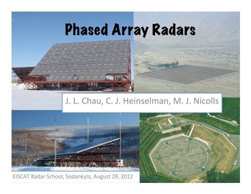
<strong>Phased</strong> <strong>Array</strong> <strong>Radars</strong><br />
J. L. Chau, C. J. Heinselman, M. J. Nicolls <br />
EISCAT Radar School, Sodankyla, August 29, 2012
Contents<br />
• Introduction<br />
• Mathematical/Engineering Concepts<br />
• Ionospheric Applications of <strong>Phased</strong> <strong>Array</strong>s<br />
• Antenna compression
Dish Antennas<br />
E θ<br />
∝ 1 r e j ( ωt−k 0r)
What is a <strong>Phased</strong> <strong>Array</strong>?<br />
- A phased array is a group of antennas whose effective (summed) radiation pattern can<br />
be altered by phasing the signals of the individual elements. !<br />
!<br />
- By varying the phasing of the different elements, the radiation pattern can be modified<br />
to be maximized / suppressed in given directions, within limits determined by !!<br />
! !(a) the radiation pattern of the elements, !<br />
! !(b) the size of the array, and !<br />
! !(c) the configuration of the array.!
Some Benefits of <strong>Phased</strong> <strong>Array</strong>s<br />
• Does not require moving a large structure around the sky for<br />
pointing. (Less infrastructure)<br />
• Fast steering. (Pulse-to-pulse)<br />
• Distributed, solid-state transmitters as opposed to single RF<br />
sources. (Less warm-up time, no need for complex feed system,<br />
elimination of single-point failures)<br />
• These features allow for:<br />
• Remote operations<br />
• Graceful degradation / continual operations<br />
• Impact on ionospheric research:<br />
• Elimination of some time-space ambiguities<br />
• Ability to “zoom-in” in time<br />
• Long durations runs (e.g., IPY)
Some Benefits of <strong>Phased</strong> <strong>Array</strong>s (2)<br />
• Non-ionospheric scientific benefits<br />
• Radio astronomy - affordable way to achieve spatial<br />
resolutions of a few arc minutes or better<br />
• Aperture real-estate - directly associated with cost of<br />
system. E.g., consider a square kilometer dish versus a square<br />
kilometer array<br />
• Non-scientific benefits<br />
• Conformity of a phased array to the “skin” of a vehicle/<br />
aircraft<br />
• Surveillance/tracking - can both survey and track 1000s of<br />
objects<br />
• Communication/downlink? - small satellites
History / Technology <br />
• Originally developed during WWII for aircraK landing <br />
• Now used for a plethora of military <br />
applicaMons <br />
• Applied to radio astronomy in 1950’s <br />
NRAO/AUI<br />
NRAO/AUI<br />
NRAO/AUI<br />
lofar.org<br />
skatelescope.org
<strong>Phased</strong> <strong>Array</strong>, λ/2 spacing
Hertzian Dipole<br />
r far-field<br />
≥ D2<br />
λ
Far-field vs. Near-field: Power<br />
∝ r<br />
∝1/ r 2<br />
Jicamarca example
Far-field vs. Near-field: Phase<br />
Near –field<br />
Need focusing<br />
Jicamarca example
Hertzian Dipole (2)
Folded Dipoles<br />
Other Elemental Antennas<br />
L/2 <br />
Current distribution on element is ~standing wave<br />
- analogous to open-ended transmission line<br />
Ground plane<br />
Monopole<br />
Same concept, twice the directivity<br />
(radiation resistance halved)<br />
E.g., AM Radio<br />
L/2 <br />
Ground plane<br />
Image antenna<br />
Driven<br />
Yagi Antenna<br />
“Parasitic” antenna (coupled elements)<br />
Director(s) slightly shorter, reflector(s) slightly longer than<br />
driven element - higher gain<br />
Current distributions must in general be solved for numerically Directors<br />
Reflector
0.25 λ, In phase, Out of phase (180 o ), 90 o<br />
Phase and Separation effects
0.50 λ, In phase, Out of phase (180 o ), 90 o<br />
Phase and Separation effects
1.00 λ, In phase, Out of phase (180 o ), 90 o<br />
Phase and Separation effects
Rectangular Planar <strong>Array</strong> <br />
Linear x array <br />
Linear y array <br />
2<br />
m<br />
-2 -1<br />
1<br />
0<br />
0<br />
1 2<br />
-1<br />
Note: No “-‐z” computed! <br />
-2<br />
n
The Fourier Analogy<br />
<strong>Array</strong> factor in spatial<br />
z domain<br />
<strong>Array</strong> factor can be<br />
interpreted as DFT<br />
of weighting factors<br />
Inverse DFT - principle of<br />
many array design methods<br />
(analogous to FIR filter design)
Visible Region and Grating Lobes<br />
Recall<br />
(1d array pointed<br />
broadside):<br />
Can see that:<br />
Visible Region <br />
Values of Farray repeat -<br />
Grating Lobes<br />
Grating lobes are analogous to classical undersampling (spectral aliasing).
Back to linear x array:<br />
Uniform, Linear <strong>Array</strong><br />
If weights are uniform:<br />
Sinc funcMon, comes from <br />
DFT of rectangular window <br />
Note that the larger the array, the <br />
narrower the beam HPBW ≈ λ/D
0.25 λ <br />
0.50 λ <br />
1.00 λ
2.00 λ <br />
4.00 λ <br />
10.0 λ
Steering and Grating Lobes<br />
For arbitrary steering direction:<br />
For no grating lobes,<br />
Modified Visible Region <br />
Also note that beam<br />
broadens as<br />
beam is steered<br />
as
Method of Moments<br />
(mutual coupling)
Mutual Coupling / Impedance <br />
• <strong>Array</strong> gain - related to gain of individual element.<br />
• Gain of isolated element very different from element gain within array.<br />
• Element pattern will also vary across array.<br />
• Actual element gain usually not known - must be simulated/measured.<br />
For an N element array:<br />
Mutual impedance <br />
Self impedance <br />
• Solve for I<br />
• Compute Poynting vector<br />
• Use this to compute radiation pattern<br />
• Important to minimize mutual coupling -> Can cause problems (standing waves “hot spots”, etc.
AMISR (PFISR, RISR-N, RISR-C)<br />
• Jicamarca - <strong>Phased</strong> array with very large collecting area, but:<br />
• (a) “Passive”, (b) Modular but not portable, (c) Fixed pointing<br />
• MU Radar - Active phased array, but not good for IS<br />
• AMISR - “Modern” Incoherent Scatter Radar constructed by the NSF
AMISR (2)<br />
• wavelength ~67 cm<br />
• elements separated by less than a wavelength<br />
Boresight<br />
y<br />
x<br />
~16 o
• Recall: Grating lobes will appear when beam is scanned far enough - makes it impossible<br />
to do incoherent scatter science beyond certain scanning limit<br />
• Recall: Gain pattern will vary with scan direction<br />
Boresight<br />
Should have seen an equation like:<br />
AMISR (3)<br />
System Constant becomes<br />
dependent on look direction<br />
350 km, 1 x 10 11 , 10%<br />
Theoretical<br />
grating lobe<br />
limits
AMISR (4) Plasma Line calibration<br />
Plasma Line CalibraMon
AMISR (5) Plasma Line Calibration
AMISR (6) Electric field Estimation
PFISR: 4D Aurora<br />
Latitude / Altitude<br />
Cross Section!<br />
Altitude / Time<br />
Cross Section!<br />
Three-Dimensional Visualization!<br />
Latitude / Longitude<br />
Cross Section!
Interferometry at Jicamarca<br />
Meteor-heads: SNR and Configuration<br />
• Jicamarca detects ~1 meteor <br />
head/sec around sunrise. <br />
• Using interferometry and <br />
special signal processing, we <br />
can determine directly: <br />
absolute velociMes and <br />
deceleraMons, where they are <br />
coming from, range and Mme of <br />
occurrence, SNR. <br />
[from Chau and Woodman, 2004]
Meteor-heads: Where do they come from?<br />
• Most meteors come from the <br />
Apex direcMon. The dispersion <br />
around the Apex is ~18 o transverse <br />
to EclipMc plane, and ~8.5 o in <br />
heliocentric longitude. Both in the <br />
Earth iniMal frame of reference. <br />
[from Chau and Woodman, 2004]
Antenna Compression: Motivation<br />
• Use high power with wide beams (imaging<br />
work, spaced antenna, aspect sensitivity<br />
measurements, etc.)<br />
• Some systems have the high power<br />
transmitters, but single antenna modules do<br />
not support such a high power (e.g.,<br />
Jicamarca). Other systems have distributed<br />
power (e.g., MU, MAARSY, AMISR)<br />
• Approaches:<br />
– Parabolic phase front (like Chirp)<br />
– Binary phase coding
Parabolic phase front: Details<br />
• Recall<br />
• Wider beams can be obtained by using parabolic<br />
phase fronts.
-10<br />
-3<br />
!y [ o ]<br />
!y [ o ]<br />
4<br />
2<br />
0<br />
-2<br />
-4<br />
4<br />
2<br />
0<br />
(a) On-axis (32214)<br />
-4 -2 0 2 4<br />
!x [ o ]<br />
-30<br />
-20<br />
Antenna compression at PFISR<br />
(c) On-axis (24513)<br />
-3<br />
-3<br />
-20<br />
!y [ o ]<br />
!y [ o ]<br />
4<br />
2<br />
0<br />
-2<br />
-4<br />
4<br />
2<br />
0<br />
-40<br />
-40<br />
(b) Amp-Phase<br />
-10<br />
-20<br />
-30<br />
-30<br />
-40<br />
-20<br />
-4 -2 0 2 4<br />
!x [ o ]<br />
-30<br />
(d) On-axis (24513)<br />
-40<br />
-20<br />
-10<br />
-3<br />
-20<br />
-40<br />
• Wide beam ~3 times<br />
wider!<br />
• Determine which<br />
meteors in the narrow<br />
beam are coming<br />
from sidelobes (~15<br />
%)<br />
• Increase number of<br />
large cross-section<br />
meteor detections<br />
-2<br />
-4<br />
-30<br />
-4 -2 0 2 4<br />
!x [ o ]<br />
-2<br />
-4<br />
-30<br />
-4 -2 0 2 4<br />
!x [ o ]<br />
[from Chau et al., 2009]
Antenna Compression:<br />
Complementary 2D Binary Coding<br />
• Evolution from 1D complementary codes (A<br />
and B).<br />
• Different sets are obtained by finding all<br />
combinations of A and B (i.e., AA, BB, AB, BA).<br />
• Transmission is performed with each 2D code.<br />
• Decoding is performed by adding the second<br />
order statistics of each code, the results is<br />
equivalent to using one module for<br />
transmission.
Binary coding : Antenna Codes<br />
A\A 1 1 1 -1 1 1 1 -1 A/B<br />
1 1 1 1 -1 1 1 1 -1 1<br />
1 1 1 1 -1 1 1 1 -1 1<br />
1 1 1 1 -1 -1 -1 -1 1 -1<br />
-1 -1 -1 -1 1 1 1 1 -1 1<br />
1 1 1 -1 1 1 1 -1 1 1<br />
1 1 1 -1 1 1 1 -1 1 1<br />
-1 -1 -1 1 -1 1 1 -1 1 1<br />
1 1 1 -1 1 -1 -1 1 -1 -1<br />
B/B 1 1 -1 1 1 1 -1 1 B\A<br />
[from Woodman and Chau, 2001]
Binary coding: Antenna Patterns
Binary coding: EEJ Results at<br />
Jicamarca<br />
(before and after adding statistics)<br />
[from Chau et al., 2009]
What are the Measurement<br />
Improvements<br />
• Inertia-less antenna pointing<br />
– Pulse-to-pulse beam<br />
positioning<br />
– Supports great flexibility in<br />
spatial sampling<br />
– Helps remove spatial/temporal<br />
ambiguities<br />
– Eliminates need for<br />
predetermined integration (dish<br />
antenna dwell time)<br />
– Opens possibilities for in-beam<br />
imaging through, e.g.,<br />
interferometry