An Adaptive Blind Channel Estimation of OFDM System by ... - SERSC
An Adaptive Blind Channel Estimation of OFDM System by ... - SERSC An Adaptive Blind Channel Estimation of OFDM System by ... - SERSC
International Journal of Hybrid Information Technology Vol.2, No.4, October, 2009 An Adaptive Blind Channel Estimation of OFDM System by Worst Case H∞ Approach 1 P.V.Naganjaneyulu and 2 Dr. K. Satya Prasad 1 Professor, Department of ECE, Guntur Engineering College, Guntur, A.P, India 2 Professor of ECE & Director of Evaluation, JNTU, Kakinada, A.P, India pvnaganjaneyulu@yahoo.co.in 1 , prasad_kodati@yahoo.co.in 2 Abstract The aim of this paper is to estimate the Channel characteristics of OFDM communication system by using worst case H ∞ approach and comparing the result with existing Kalman [6] and H ∞ channel estimators [8]. This estimation criterion is different from kalman filter. These two algorithms fail because of more updation parameters like V, W and Q. In order to estimate the signal without updating factors, we are proposing this worst case H-infinity approach in which V and W are considered as worst case values (maximum). In this approach V and W are updated only once for entire recursive estimation process. This method improves the performance even for high data rate also. Keywords: Kalman Filter, H ∞ approach, Updation parameters 1. Introduction The high demand for a large volume of multimedia services in wireless communication systems requires high transmission rates [1]. However, high transmission rates may result in severe frequency selective fading and inter symbol interference (ISI), when the Bandwidth of the transmitted signal is large compared to the coherence bandwidth of the channel. Orthogonal frequency division multiplexing (OFDM) has been proposed to combat these types of channel disturbance. A proper channel estimation algorithm for the OFDM systems should capture both the time and frequency domain characteristics. This channel estimation is done in time domain by considering the channel fading factors. Serial data I/P Serial to parallel converter N-point IFFT Parallel to serial converte r Cyclic prefix converte r Figure 1. Basic Transmission Section of OFDM 1
- Page 2 and 3: International Journal of Hybrid Inf
- Page 4 and 5: International Journal of Hybrid Inf
- Page 6: International Journal of xxxxxx Vol
International Journal <strong>of</strong> Hybrid Information Technology<br />
Vol.2, No.4, October, 2009<br />
<strong>An</strong> <strong>Adaptive</strong> <strong>Blind</strong> <strong>Channel</strong> <strong>Estimation</strong> <strong>of</strong> <strong>OFDM</strong> <strong>System</strong> <strong>by</strong> Worst<br />
Case H∞ Approach<br />
1 P.V.Naganjaneyulu and 2 Dr. K. Satya Prasad<br />
1 Pr<strong>of</strong>essor, Department <strong>of</strong> ECE,<br />
Guntur Engineering College,<br />
Guntur, A.P, India<br />
2 Pr<strong>of</strong>essor <strong>of</strong> ECE &<br />
Director <strong>of</strong> Evaluation, JNTU,<br />
Kakinada, A.P, India<br />
pvnaganjaneyulu@yahoo.co.in 1 , prasad_kodati@yahoo.co.in 2<br />
Abstract<br />
The aim <strong>of</strong> this paper is to estimate the <strong>Channel</strong> characteristics <strong>of</strong> <strong>OFDM</strong> communication<br />
system <strong>by</strong> using worst case H ∞ approach and comparing the result with existing Kalman [6]<br />
and H ∞ channel estimators [8]. This estimation criterion is different from kalman filter. These<br />
two algorithms fail because <strong>of</strong> more updation parameters like V, W and Q. In order to estimate<br />
the signal without updating factors, we are proposing this worst case H-infinity approach in<br />
which V and W are considered as worst case values (maximum). In this approach V and W are<br />
updated only once for entire recursive estimation process. This method improves the<br />
performance even for high data rate also.<br />
Keywords: Kalman Filter, H ∞ approach, Updation parameters<br />
1. Introduction<br />
The high demand for a large volume <strong>of</strong> multimedia services in wireless communication<br />
systems requires high transmission rates [1]. However, high transmission rates may result in<br />
severe frequency selective fading and inter symbol interference (ISI), when the Bandwidth <strong>of</strong><br />
the transmitted signal is large compared to the coherence bandwidth <strong>of</strong> the channel. Orthogonal<br />
frequency division multiplexing (<strong>OFDM</strong>) has been proposed to combat these types <strong>of</strong> channel<br />
disturbance. A proper channel estimation algorithm for the <strong>OFDM</strong> systems should capture both<br />
the time and frequency domain characteristics. This channel estimation is done in time domain<br />
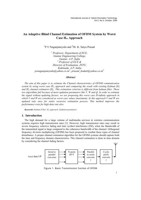
<strong>by</strong> considering the channel fading factors.<br />
Serial data I/P<br />
Serial to<br />
parallel<br />
converter<br />
N-point<br />
IFFT<br />
Parallel<br />
to serial<br />
converte<br />
r<br />
Cyclic<br />
prefix<br />
converte<br />
r<br />
Figure 1. Basic Transmission Section <strong>of</strong> <strong>OFDM</strong><br />
1
International Journal <strong>of</strong> Hybrid Information Technology<br />
Vol.2, No.4, October, 2009<br />
Cyclic<br />
prefix<br />
remove<br />
r<br />
Serial to<br />
parallel<br />
converter<br />
N-point<br />
FFT<br />
Parallel<br />
to serial<br />
converter<br />
Figure 2. Basic Receiving Section <strong>of</strong> <strong>OFDM</strong><br />
Serial data o/p<br />
2. Overview <strong>of</strong> <strong>OFDM</strong> communication system<br />
<strong>OFDM</strong> is multicarrier transmission technique, where the spacing between two adjacent<br />
carriers is identical to the inverse <strong>of</strong> the symbol period. To generate <strong>OFDM</strong> successfully the<br />
relationship between all the carriers must be carefully controlled to maintain the orthogonality<br />
<strong>of</strong> the carriers. For this reason, <strong>OFDM</strong> is generated <strong>by</strong> firstly choosing the spectrum required<br />
based on the input data. Each carrier to be produced is assigned some data to transmit. The<br />
required amplitude and phase <strong>of</strong> the carrier is then calculated based on the modulation scheme<br />
(typically differential BPSK, QPSK, or QAM). The required spectrum is then converted back to<br />
its time domain signal using an Inverse Fourier Transform. In most applications, an Inverse<br />
Fast Fourier Transform (IFFT) is used. The IFFT performs the transformation very efficiently,<br />
and provides a simple way <strong>of</strong> ensuring the carrier signals produced are orthogonal. The Fast<br />
Fourier Transform (FFT) transforms a cyclic time domain signal into its equivalent frequency<br />
spectrum. Finding the equivalent waveform, generated <strong>by</strong> a sum <strong>of</strong> orthogonal sinusoidal<br />
components, does this. The amplitude and phase <strong>of</strong> the sinusoidal components represent the<br />
frequency spectrum <strong>of</strong> the time domain signal. <strong>OFDM</strong> has several advantages like less inter<br />
symbol interference, simplicity <strong>of</strong> channel equalization, efficient use <strong>of</strong> spectrum, etc.<br />
3. Introduction to channel estimation procedures<br />
The channel estimation procedure considers a Radio communication system in which<br />
training sequences are sent periodically to form data based estimates <strong>of</strong> the channel. The<br />
channel is assumed to be invariant over the time span <strong>of</strong> the training sequence being sent over<br />
the channel. This, in general is undesirable since any such increase would result in more waste<br />
<strong>of</strong> channel bandwidth, which is better utilized for sending data rather than training information.<br />
The channel estimation algorithm presented in this section improves on the data based estimate<br />
without decreasing channel throughput. Impairments in a wireless channel are unknown and<br />
most likely time-variant. Methods that do not depend on precise knowledge <strong>of</strong> the channel<br />
characteristics should be more effective and robust for performing the channel. In the designs <strong>of</strong><br />
channel estimators in which the estimator gains are optimized using a minimum error variance<br />
criterion [6] (the Kalman filtering approach) and a minimum estimation error spectrum criterion<br />
[8] (the mod H ∞ filtering approach) are presented. The Kalman approach is a covariance<br />
minimization problem while the mod H ∞ approach is a minimization problem where the<br />
maximum “energy” <strong>of</strong> the estimation error <strong>of</strong> overall disturbances is minimized.<br />
3.1 Briefing about kalman filtering<br />
2
International Journal <strong>of</strong> Hybrid Information Technology<br />
Vol.2, No.4, October, 2009<br />
The kalman filter is a tool that can estimate the variables <strong>of</strong> a wide range <strong>of</strong> processes. In<br />
mathematical terms we would say that a kalman filter estimates the states <strong>of</strong> a linear system.<br />
The kalman filter not only works well in practice, but it is the one that minimizes the variance<br />
<strong>of</strong> the estimation error. In order to use a kalman filter to remove noise from a signal, the process<br />
that we are measuring must be able to be described <strong>by</strong> a linear system. Kalman filter is an<br />
optimal recursive linear estimator. It processes all available measurements, regardless <strong>of</strong> their<br />
precision, to estimate the current value <strong>of</strong> the variables <strong>of</strong> interest with use <strong>of</strong> knowledge <strong>of</strong> the<br />
system noises, measurement errors and any available information about initial conditions <strong>of</strong> the<br />
variables <strong>of</strong> interest.<br />
<strong>Estimation</strong> <strong>of</strong> a random vector Y based on all observations at once, it is <strong>of</strong>ten beneficial to<br />
estimate Y from a subset <strong>of</strong> the observations and then update the estimator with new<br />
observations. This is done recursively with observation random vectors X 0 , X 1 , X 2 … <strong>An</strong> initial<br />
linear estimator for Y is based on ˆX ; this initial estimator is used in conjunction with X<br />
0<br />
1 to<br />
obtain the optimal linear estimator based on ˆX 0<br />
and ˆX ; and this procedure is recursively<br />
1<br />
performed to obtain linear estimators for Y based on X 0 , X 1 … X j , for j= 1, 2… It is used in the<br />
recursive estimation <strong>of</strong> time varying signals<br />
3.2 Briefing about H-Infinity filtering process<br />
A robust H-infinity channel estimation algorithm is proposed to estimate the channel fading<br />
in the time domain. The H-infinity approach differs from the traditional approach such as the<br />
Kalman estimation in the following two respects.<br />
No a prior knowledge <strong>of</strong> the noise source statistics is required. The only assumption is<br />
that the noise has finite energy.<br />
The estimation criterion is to minimize the worst possible effect in the estimation error<br />
(including channel modeling error and additive noise).<br />
3.3 Equations related to the H-infinity and kalman filter<br />
Let us recall that the Kalman filter estimates the states x <strong>of</strong> a linear dynamic system [4],<br />
defined <strong>by</strong> the equations<br />
xK<br />
1<br />
Axk<br />
Buk<br />
wk<br />
…… (1)<br />
yK<br />
Cxk<br />
zk<br />
……. (2)<br />
Where A, B, and C are known matrices; k is the time index; x is the state <strong>of</strong> the system<br />
(unavailable for measurement); u is the known input to the system; y is the measured output;<br />
and w k and z k are noise. The two equations represent what is called a discrete time system,<br />
because the time variable k is defined only at discrete values (0, 1, 2…). We cannot measure the<br />
state x directly; we can only measure y directly. In this case we can use a Kalman filter to<br />
estimate the state x. The state equations <strong>of</strong> kalman filter given as follows:<br />
K<br />
xˆ<br />
T<br />
CP C S 1<br />
T<br />
k<br />
APk<br />
C<br />
k z<br />
……. (3)<br />
k 1<br />
k<br />
1<br />
Axˆ<br />
Bu <br />
K y<br />
Cxˆ<br />
<br />
… (4)<br />
k<br />
k<br />
k<br />
w<br />
Where S w and S z are the covariance matrices <strong>of</strong> w and z, K is the Kalman gain, and P is the<br />
variance <strong>of</strong> the estimation error. The Kalman filter works well, but only under certain<br />
3<br />
k<br />
k<br />
k 1<br />
T<br />
T<br />
T<br />
P<br />
<br />
AP A S AP C S CP A ... (5)<br />
1<br />
z<br />
k<br />
k
International Journal <strong>of</strong> Hybrid Information Technology<br />
Vol.2, No.4, October, 2009<br />
conditions. First, the noise processes need to be zero mean. The average value <strong>of</strong> the process<br />
noise, w k , must be zero, and the average value <strong>of</strong> the measurement noise, z k , must also be zero.<br />
This zero mean property must hold not only across the entire time history <strong>of</strong> the process, but at<br />
each time instant, as well. That is, the expected value <strong>of</strong> w and z at each time instant must be<br />
equal to zero. Second, we need to know the standard deviation <strong>of</strong> the noise processes. The<br />
Kalman filter uses the S w and S z matrices as design parameters (these are the covariance<br />
matrices <strong>of</strong> the noise processes). That means that if we do not know Sw and Sz, we cannot<br />
design an appropriate Kalman filter. The attractiveness <strong>of</strong> the Kalman filter is that it results in<br />
the smallest possible standard deviation <strong>of</strong> the estimation error.<br />
3.4 <strong>Channel</strong> estimator (objective function <strong>of</strong> H-infinity approach)<br />
The problem formulation <strong>of</strong> H ∞ approach will start as min x max w,v J where J is some measure<br />
<strong>of</strong> how good our estimator is. We can view the noise terms w and v as adversaries that try to<br />
worsen our estimate. Think <strong>of</strong> w and v as manifestations <strong>of</strong> Murphy’s Law: they will be the<br />
worst possible values. So, given the worst possible values <strong>of</strong> w and v, we want to find a state<br />
estimate that will minimize the worst possible effect that w and v have on our estimation error.<br />
This is the problem that the H infinity filter tries to solve. For this reason, the H infinity filter is<br />
sometimes called the minimax filter; that is, it tries to minimize the maximum estimation error.<br />
We will define the function J as follows:<br />
ave xk<br />
xˆ<br />
k Q<br />
J …… (6)<br />
ave w ave v<br />
4<br />
k<br />
W<br />
Where the averages are taken over all time samples k. In other words, we want to find that<br />
minimizes J, so we want to find that is as close to x as possible. But nature tries to maximize J,<br />
so we want to find noise sequences W and V that cause our estimate to be far from the true state<br />
x. The previous equation is the statement <strong>of</strong> the H infinity filtering problem. Our task is to find<br />
a state estimate that makes J small even while noise terms that make J large. The Q, W, and V<br />
matrices that are used in the weighted norms in J are chosen <strong>by</strong> designer, to obtain desired<br />
trade-<strong>of</strong>fs. For example, if we know that the W noise will be smaller than the V noise, we<br />
should make the W matrix smaller than the V matrix.<br />
3.5 Worst case channel estimator (objective function <strong>of</strong> H-infinity approach)<br />
The cost function generally defined for H ∞ is given as (6). In this so many tuning parameters<br />
are observed like Q, W and V. For every time, we need to update these tuning parameters<br />
which is complicated for high data transmission. So, the denominator <strong>of</strong> H ∞ cost function is<br />
approximated with worst case values <strong>of</strong> V and W. These are considered as V 1 and W 1 instead<br />
<strong>of</strong> average values. Then the worst case cost function becomes<br />
ave x ˆ<br />
k<br />
xk Q<br />
JOpt<br />
<br />
…. (7)<br />
w'<br />
v'<br />
W v<br />
This process repeats like 3.4 for k number <strong>of</strong> samples. Always equation (7) gives better<br />
performance than (6) because we are considering worst case values initially without updation<br />
every time. At any time, for any sample J opt < J. With this worst case designing better<br />
optimum estimation is obtained.<br />
4. Design approach<br />
k<br />
v
International Journal <strong>of</strong> Hybrid Information Technology<br />
Vol.2, No.4, October, 2009<br />
The design flow for implementing ODFM and estimation <strong>of</strong> <strong>OFDM</strong> was realized on<br />
MATLAB environment starting with random input data as input. High data rate signals should<br />
be passed through <strong>OFDM</strong> system analyze this data rate compatibility for different channel<br />
estimation algorithms mainly concentrate towards worst case H ∞ , how best estimate the<br />
characteristic <strong>of</strong> channel and the performance is compared with existing Kalman filter and H ∞<br />
filter. So with this proposed worst case H-infinity approach better result will be obtained, so,<br />
enhanced H-infinity approach cost function J is varied according to given data rate.<br />
The simulation shown is evaluated with variation in channel noise strength and varying the<br />
fading strength in the channel. The system is evaluated keeping the SNR low and high with the<br />
increase in fading strength and decreasing in the fading strength. In this result analysis is<br />
evaluated for 2 cases <strong>by</strong> using Effect <strong>of</strong> Input SNR, Effect <strong>of</strong> BER.<br />
Figure 3. SNR v/s BER Plot<br />
At 12 db 10 -7 10 -9 10 -11 At 14 3.2 2.9 2.7<br />
Figure 4. % error v/s samples<br />
Table 1.<br />
Table 2.<br />
BER <strong>of</strong> Number<br />
%error <strong>of</strong> %error <strong>of</strong><br />
SNR BER <strong>of</strong> BER <strong>of</strong><br />
%error <strong>of</strong><br />
extended<br />
<strong>of</strong><br />
h- extended<br />
Value kalman H ∞<br />
kalman<br />
H ∞<br />
samples<br />
infinity h-infinity<br />
At 6 db 10 -2.5 10 -3 10 -3.5 At 2 8.5 8.1 7.7<br />
At 10 db 10 -5 10 -6.5 10 -8<br />
At 8 8.25 7.4 6<br />
5. Conclusion<br />
In the result analysis 2 cases are studied, in each case simulation results gives analysis<br />
between % error vs. No. <strong>of</strong> samples and BER vs. SNR. All the cases are analyzed <strong>by</strong> effect <strong>of</strong><br />
input SNR and channel noise characteristics. From the simulation results we can conclude that<br />
1. With an increase in input SNR, the mean-square-error performance <strong>of</strong> worst case H ∞ ,<br />
H ∞ and Kalman estimation algorithms improves.<br />
2. The worst case H ∞ estimation algorithm outperforms the Kalman and H ∞ estimation<br />
algorithms over all the SNR range is considered.<br />
References<br />
[1] L. J. Camino Jr., “<strong>An</strong>alysis and simulation <strong>of</strong> a digital mobile channel using orthogonal frequency division<br />
multiplexing,” IEEE Trans. Commun., vol. COM-33, pp. 665–675, July 1985.<br />
5
International Journal <strong>of</strong> xxxxxx<br />
Vol. x, No. x, xxxxx, 2007<br />
[2] Low price Edition, Jochen Schiller,"Mobile communications"-Second Edition<br />
[3] Low price Edition, <strong>An</strong>dreas F. Molisch," Wide band wireless communications"<br />
[4] Low price Edition, "<strong>Adaptive</strong> filter theory" –Simon Haykin, Fourth Edition<br />
[5] D. K. Borah and B. D. Hart, “Frequency-selective fading channel estimation with a polynomial time-varying<br />
channel model,” IEEE Trans. Communications., vol. 47, pp. 862–873, June 1999.<br />
[6] I. R. Petersen and A. V. Savkin, Robust Kalman Filtering for Signals and <strong>System</strong>s with Large Uncertainties.<br />
Boston, MA: Birkhäuser, 1999.<br />
[7] R. Steele, Mobile Radio Communications. New York: IEEE Press, 1992.<br />
[8] Jun Cai, Xuemin Shen, Robust <strong>Channel</strong> <strong>Estimation</strong> for <strong>OFDM</strong> <strong>System</strong>s- <strong>An</strong> H ∞ Approach: IEEE Transactions<br />
On Wireless Communications, Vol. 3, No. 6, November 2004<br />
Authors<br />
P.V.Naganjaneyulu,<br />
B.Tech, M.E,<br />
Pr<strong>of</strong>essor, Department <strong>of</strong> ECE,<br />
Guntur Engineering College,<br />
Guntur, A.P, India<br />
pvnaganjaneyulu@yahoo.co.in<br />
Mobile: +91-9490650030<br />
Dr.K.Satya Prasad<br />
Pr<strong>of</strong>essor in ECE,<br />
Director <strong>of</strong> Evaluation<br />
JNTU, Kakinada,<br />
A.P, India.<br />
Prasad_kodati@yahoo.co.in<br />
Mobile: +91-9912240855<br />
6


